The Relationship between Economic Growth, Budget balance ...

The Relationship between Economic Growth,

Budget balance, Tax revenue and Government

Debt

Seyedeh Fatemeh Alavi Abkenar

Submitted to the

Institute of Graduate studies and research

In partial fulfillment of the requirements for the Degree of

Master

of

Business Administration

Eastern Mediterranean University

July 2013

Gazimağusa, North Cyprus

iii

ABSTRACT

The main focus of this thesis is to investigate the impact some selected macroeconomic

variables such as gross capital formation, inflation, trade openness, budget balance,

central government debt and tax revenue on growth percentage of GDP of four selected

countries from South America, North America and Middle East for the period of 1995-

2010. In this study first we examined the relationship and impact of gross capital

formation, inflation, trade openness together with budget balance on growth percentage

of GDP. Second stage was examining the impact of gross capital formation; inflation and

trade openness together with tax revenue on growth percentage of GDP of each country

and last part of individual country regression belong to investigating the impact of gross

capital formation, inflation, trade openness and stock of public debt on economic growth

of each country separately. Afterward we employed panel data, pooled white cross-

section time series to investigate the long run impact of relationship examined separately

for our countries as a group. Result of our work indicates there’s positive correlation

between gross capital formation and growth percentage of GDP. The same result has

been proofed for nexus between budget balance and growth percentage of GDP.

Keywords: Macroeconomic Variables, Growth Percentage of GDP, South America,

North America, Middle East.

iv

ÖZ

Bu tez, Guney Amerika, Kuzey Amerika ve Ortadogu ulkelerinin 1995-2000 yillari

arasindaki enflasyonun, ticari serbestliginin,butce dengesinin,gayri safi sermaye

olusumunun, devlet borcunun ve vergi gelirlerinin buyumeye etkisini arastirmayi

amaclamaktadir. Bu arastirmada oncelikle gayri safi sermaye olusumunun, enflasyonun

ve ticari serbestligin gayri safi milli hasiladaki buyumeye etkisini inceledik. Ikinci

asamada ise enflasyonun, ticari serbestligin, butce dengesinin, gayri safi sermaye

olusumunun, devlet borcunun ve vergi gelirlerinin her ulke icin ayri ayri olmak

kosuluyla, gayri safi milli hasilanin buyumeye etkisini inceledik. Son kisimda ise bu

etkenlerin ve devlet borcunun bu ulkelerdeki iktisadi buyumeye olan etkilerini arastirdik.

Daha sonra capraz kesitli frekans dagilimli inceleme methodu ile ulkeleri grup halinde

inceleyerek, uzun vadedeki etkilerini arastirdik.Incelemelerimizin ve analizlerimizin

sonucunda gayri safi sermaye olusumu ile gayri safi milli hasiladaki yillik buyumede

pozitif bir korelasyon oldugunu gorduk. Ayni bagin butce dengesi ve gayri safi mili

hasila arasinda da oldugunu ispatlamis olduk. Ancak,ticari serbestligin, enflasyonun

devlet borcunun ve vergi gelirlerinin buyume icin pozitif degil, aksine negative bir

yansima yaptigini da ispatlamis olduk.

Anahtar Kelimeler: makroekonomik degiskenler, gayri safi milli hasila buyumesi,

guney amerika, kuzey amerika, ortadogu

v

This study is dedicated to my beloved parents for all they

sacrificed to support me during my study

vi

ACKNOWLEDGMENTS

I would like to express the deepest appreciation to my supervisor Prof. Dr.

SerhanÇıftçıoğlu who gave me the opportunity of being advised by him and provided me

useful comments and engaged me to the research world through the process of this

master thesis.

I would also like to thank my defense participants who willingly shared their precious

time to attend this session.

And I want to share my special gratitude to my beloved Family and best friends; Antony

Kimondo, Charles Machatha and PhD. DavoodKhodadad who supported me in whole

process and shared their concerns and knowledge during this thesis.

This work wouldn’t be complete and successful without help of all of you.

vii

TABLE OF CONTENTS

ABSTRACT…………………...…………………………………………………….iii

ÖZ ……………………………………………………………………………….…..iv

DEDICATION…………………………………………………………....………….v

ACKNOWLEDGMENTS…………………………………………………………...vi

1 INTRODUCTION.…………………………….....………………………..………1

2 LITERATURE REVIEW………………….……………………………………....5

2.1 Impact of Trade Openness on Economic Growth……………...…………….…….…5

2.1.1 Impact of Export on Economic Growth………………...……….….…7

2.1.2 Impact of Import on Economic Growth……………………...………..9

2.2 Impact of Public Debt on Economic Growth…………..……………………….…..10

2.3 Impact of Inflation on Economic Growth……………………………………………11

2.4 Impact of Tax Revenue on Economic Growth……………………………………….14

2.5 Impact of Gross Capital Formation on Economic Growth………………………….16

2.6 Impact of Budget Balance on Economic Growth……………………………………17

3 THEORIES OF ECONOMIC GROWTH…………………………………………20

3.1 Classical Growth Theory……………………………………………………………..21

3.2 Neoclassical Growth Theory…………………………………………………………21

viii

3.3 New Growth Theory ......................................................................................................... 23

3.4 New Growth Theory Versus Classical Theory of Economic Growth ............................... 24

3.5 Neoclassical Growth Theory Versus Classical Growth Theory........................................ 24

4 DATA AND DATA METHODOLOGY ...................................................................... 25

4.1 Regression Analysis .......................................................................................................... 25

4.2 Panel Data Regression ....................................................................................................... 27

4.3 OLS Method ....................................................................................................................... 28

5 INDIVIDUAL REGRESSION FOR EACH COUNTRY ............................................ 31

5.1 Data ................................................................................................................................... 31

5.2 Data Analysis ..................................................................................................................... 31

5.3 Influence of Investment, Inflation Rate, Trade Openness and Budget Balance on Growth

Percentage of GDP .................................................................................................................. 32

5.3.1 Chile ............................................................................................................. 33

5.3.2 Mexico ......................................................................................................... 35

5.3.3 Turkey .......................................................................................................... 36

5.3.4 Israel ............................................................................................................. 37

5.4 Influence of Capital Accumulation, Inflation Rate, Tax Revenue and Trade Openness on

Growth Percentage of GDP ..................................................................................................... 38

5.4.1Chile ............................................................................................................. 39

5.4.2 Mexico ........................................................................................................ 41

5.4.3 Turkey ........................................................................................................... 42

ix

5.4.4 Israel .............................................................................................................. 43

5.5 Influence of Capital Accumulation, Inflation Rate, Trade Openness and Stock of Public

Debt on Growth Percentage of GDP ....................................................................................... 45

5.5.1 Chile……………………………………………………………………....46

5.5.2 Mexico..……….……………………….…………………………..……..47

5.5.3Turkey..………………………...………………………………………….48

5.5.4 Israel………………………………………………………………………49

6 POOLED REGRESSION ANALYSIS ........................................................................ 51

6.1 Influence of Gross Capital Formation, Inflation, Trade Openness and Budget Balance on

Growth Rate of Sample Countries as One Group ………...……………………………...…..51

6.2 Impact of Gross Capital Formation, Inflation, Tax Revenue and Trade Openness on

Growth Percentage of GDP of our Countries as a Group… ……………………………...….53

6.3 Impact of Gross Capital Formation, Inflation, and Stock of Public Debt and Trade

Openness on Growth Percentage of GDP of Our Countries as a Group ............................... ..55

7 CONCLUSION ............................................................................................................. 57

REFRENCES ................................................................................................................. ..60

APPENDIXES ……………………………...……………………………………….....63

Appendix A: Individual Regression Results ………….………….......…………….64

Appendix B: Pooled Regression Results……......…….…………………...…….…76

1

Chapter 1

INTRODUCTION

Studies of macroeconomic, particularly theoretical and practical researches were concern

of economists and governors. Study of macroeconomic variables helps understanding of

nature of whole economy. Knowing impact of each variable involve in macroeconomic

theories and way they influence the economy helps finding solutions to improve national

economic performance of one‟s country through editing or changing economic policies.

“Working with macroeconomic concepts is a bare necessity in order to contribute to

solutions of great problems of our time”. (Tinbergen)

This research main concern is on economic growth and particular selected variables that

affecting this indicator, and investigating the size of their effect on growth of our selected

countries. As you know there has been huge emphasis on finding sources of economic

growth which actually can define macroeconomic performance of various countries. Hence

there have been loads of studies on determining factors affecting economic growth,

number of which can‟t be all investigated in one research work so here in this paper we are

going to put stress on some of most important ones for instance:

- Capital accumulation, known also as investment is one of the most important

macroeconomic variable in defining growth of economy. Theories emphasize on positive

2

correlation between this indicator and growth of nations. “The accumulation of capital

builds a simple model of economic growth based on the capitalist rule of the game”. Joan

Robinson

- Inflation rate left no doubt for being harmful for an economy. Based on Keynesian

view, inflation will lead to high fluctuation of national currency which decreases the

positive performance of an economy. However in this area there have been different views

about the impact of inflation, Tobin and Sidrausky (1960‟s) point of view was against of

those Keynesian, believing in positive impact of inflation on growth in both short and long

run. Based on their investigation they found increase in inflation will cause transfer of

wealth from money into physical capital therefore it increases capital accumulation.

- Trade openness and its relationship with growth has been subject of investigation

for Decades. Researchers have different point of view about this nexus, some insisting on

positive relationship between these two variables and some disagree. Barro and Sala-i-

Martin (1995) are among those who believed Trade liberalization will open way for

countries to access Technology of rest of the world, some others like Chang, Kaltani,

Loayza (2005) saw this relationship positive in way it helps allocation of resources around

the world. Among those who disagree and doubt about the positive nexus between these

variables were Krugman (1994) and Rodrik and Rodriguez (2001).

3

We have discussed the rest of our variables in detail in literature review.

Countries of our investigation are also having distinguishing characteristic that mad us

interested in checking their growth behavior. Four countries are subject of our research,

one of them Chile from South America the other one Mexico from North America and

Turkey and Israel from Middle East. These countries have unique and interesting features,

all of them being member of OECD, they are showing notable growth during last decade.

Chile being first country from Latin America joining OECD, has ranked 30th

country in the

world and first of its region in competitiveness. Mexico has been growing fast after crisis

in 1994, almost the same time period we are doing our research, the country is supporting

private ownerships and is Export oriented and does almost 90 percent of its trade through

free trade agreement (FTAS) and about 40 countries around the world are target of their

trade including Israel. Turkey has been in rapid growth line for past few years and is

considered as emerging market as those of MEXICO and CHILE. Turkey is one of the

world newly industrialized countries. It has been among those few countries which

financial sectors showed growth on time of world economic crisis and its largest country in

OECD in terms of growth. Our last country of research is Israel that has been ranked 26th

competitive economy in the world, and is highly developed country with notably small

population and size comparing to other countries of our research.

The goal of this research is to investigate the impact of our variables (Gross capital

formation, Inflation, Trade openness, Tax revenue, Budget Balance and Stock of public

4

debt) on Growth percentage of GDP of countries selected during 1995-2010 by applying

series of simple and multiple regressions.

In next chapters you can find more detailed information about this research paper. This

Thesis consist of eight chapters, next chapter is where you can find more detail information

about the concept of each variable and the previous studies on each of them and their

impacts whether positive or negative in growth. Third chapter is about the theories of

growth and brief explanation about factors affecting growth through each theory. Fourth

chapter is introduction of methodologies and types of regressions that will be used during

the work. Chapter five is showing the regression results for each country separately.

Chapter six is where you can find pooled regression result and chapter seven is our last

chapter that includes the conclusion of the research.

5

Chapter 2

LITERATURE REVIEW

In literature economic growth has been defined as an improvement in economy,

production, services and quality of life of people within that economy from one period of

time to another. This concept can be measured in two ways, nominal and real term. Annual

percent of GDP (gross domestic product) is a way of measuring how an economy is

moving toward being advance. World‟s GDP growth announced 3.7% in 2011. There are

factors that can have impact on real GDP of a nation, and there has been huge amount of

research to investigate these factors and the way they slow down or speed up this process.

In this thesis we chose some of the effective indicators and investigated the previous

studies and summarized some of their impacts on economic growth.

1.1 Impact of Trade Openness on Economic Growth

It‟s a fact that trade liberalization has some positive effects on growth of whole world

economy as it helps in efficiency of allocation of resources between different countries but

how to balance and gain equitability is the important part of this game.

Policies in Trade openness play important role, studies show that those countries applying

regional trade liberalization (trade agreement between countries of the same region) have

6

lower rate of growth and investment and Multilateral or unilateral trade liberalization will

improve growth performance (Anthony P.Thirlwall, 2000).

While trade openness is advised for whole world, most of countries have tendency toward

import when it comes to trade liberalization, which will lead to trade deficit and lack of

trade balance, one of the factors that can cause low economic growth in future.

Trade balance is a lagging indicator which shows net difference between value of exports

and import and it also declare whether the country has trade deficit or surplus.

Trade deficit can be harmful for economy of the country in long-run; some of the negative

impacts can be listed as devaluation of local currency and increase of foreign debt. For

ages analysis use to believe that trade openness has positive correlation with economic

growth, by Rodriguez and Rodrik increase more concerns on difficulties in measuring

openness, statistically sensitive specifications and collinearity of protectionist policies and

some poorly executed policies on developing economies.

Previous studies from Thirwall and Santos-Paulino (2004) shown the impacts of Trade

liberalization on countries before and after liberalization, which lead to the fact that trade

liberalization has far more greater impact on import than before liberalization (closed

economic period). They also found that trade liberalization has more positive effect on

import than export, after trade liberalization policies has been applied, increase in import

according to their research was about 6% per year while export increased only by 2%.

7

Two other researchers called Dollar and Kray on 2004 also did research on the impact of

trade liberalization on globalizing developing countries as compar to non- globalized and

Developing countries. According to their findings all countries of their research has shown

growth in their real income while globalizing – developing countries were having leading

growth speed than other two groups with the growth about 5% per capital and non-

globalized developing countries had growth rate of only 1.4%. Based on their findings they

emphasized that globalizing developing countries are having competition with rich

countries growth of which was over 2.2%. In this competition non globalized countries are

far behind globalizing in terms of growth.

Almost all studies have shown that trade liberalization will lead to growth in real income

and per capital growth however there is essential need of controlling and applying some

policies that can keep the balance between export and import. In our paper we found trade

openness via summing import percentage of GDP and export percentage of GDP so we

found it interesting to provide some information about impact of each variable separately

on Economic growth.

1.1.1 Impact of Export on Economic Growth

Export is an undeniable factor in pushing a country toward growth and wealth, as it effects

economy of a country in different aspects such as increase in quality of goods and services

produced within a country, competitiveness among different sectors inside or between

countries, industrial development, efficient management due to competitive pressure, lower

foreign exchange rate (as exporter country gets more of foreign currency and brings it back

to its economy), high purchasing power of the nation and lower rate of unemployment.

8

Loads of researches has been conducted to evaluate the importance of export for an

economy, for instance Bela Balassa, William Tyler, Gershon Feder and Rostam Kavoussi

investigated correlation between export and economic Growth Via other economic growth

determining fundamentals such as Labor and capital in production-type function with

investment (capital formation), manufacturing and total exports.( Swarna D. DUTT and

Dipak Ghosh,1996)

According to Rodrigo time series should reflect the effect of policy in the relationship

between export and growth, in his Article he also mentions in countries following inward

looking strategy, exports should not have a positive impact on growth while countries

applying outward –strategy export should increase economic growth since the policy is

linking the country‟s growth rate to world market evolution (Rodrigo Navia, 1997).

Chow studied 8 countries in which just one country (MEXICO) showed positive

relationship between export and growth and Argantina showed no nexus between export

and Growth. In illustrating the impact of Export on growth using test of causality is

important, tests like Granger causality (Granger 1969) that can determine whether one time

series data is useful in forecasting another.

Research on Chile case (1974-1993) using causality test showed that there is Granger

causality from export growth to growth in GDP. In this period the country used Export

promotion policy while from (1950-1973) used import substitution and there found no

granger causality between these two variables. (Rodrigo Navia, 1997)

9

1.1.2 Impact of Import on Economic Growth

While some studies showing the negative impacts of import, some are supporting it and

emphasizing on the positive effects of it. They believe that import will lead to growth for

instance endogenous growth model reveals this positive effect on long-run economic

growth, since it provides domestic firms with access to needed intermediate and foreign

technology (Coe and Helpman, 1995).

Growth in imports can serve as a medium for the transfer of growth-enhancing foreign

R&D knowledge from developed countries to developing countries (Lawrence and

Weinstein, 1999; Mazumdar,2000). According to an investigation on impact of import on

growth in France, Using (VEC and improved-VEC and geostatistical methods) results

showed existence of long-run unidirectional causality from export and import to economic

growth.(Arshia Amiri, UIF-G Gerdtham)

Increase in economic activity on the other hand will cause increase in import because high

real income in a country usually leads to higher consumption so there is a direct

relationship between economic growth and import. (Rivera-Batiz, 1985)

Most of recent endogenous models emphasized on importance of import as a channel for

foreign technology and knowledge to flow into domestic economy. (Grossman and

Helpman, 1991; Lee, 1995: 91-110; Mazumdar, 2001: 209-224)

10

1.2 Impact of Public Debt on Economic Growth

Here we are going to concentrate on effects of debt on growth in long run. According to a

research done by IMF, public debt can increase and exist because of various reasons some

of which can be named as: “long-term interest rates, high inflation rate, great uncertainty

and possibly higher future distortionary taxation and sensitiveness to crisis.

Although negative impacts of debt on growth is undeniable but there is not enough

systematic evidence to show us to which extent large debts can decrease the potential

growth.

The effect of debt on growth can carry on simultaneity bias meaning it‟s possible that debt

can have unfavorable effects on growth “low growth for some reasons can be unrelated to

debt and lead to high debt, or in other conditions both debt and growth could be affected by

a third variable.” Study done by Kumar Monmohan and Woo Jaejoon,2010, shows adverse

relationship between two variable “public debt” and “economic growth”, holding other

factors affecting growth fixed, on increase on debt by 10% decrease the annual real per

capital GDP growth by 0.2% and however this impact is smaller in advanced economies.

And according to the same research they found out that this slowdown in economic growth

has larger effect on decline of labor productivity growth, as a result of lower investment

and slower growth of capital stock.

Channels and Existing studies:

Channels that can have negative effect on medium and long run growth can be listed as:

11

- High public debt, which can effect capital accumulation and growth through higher

interest rate in long-term (Gale and Orzag, 2003; Baldacci and Kumar,2010)

- Higher future destructive taxation, (Barro, 1979; Dotsey, 1994)

- Inflation, (Sargent and Wallance, 1981; Barro, 1995; Cochrane, 2010)

- High uncertainty about future and policies.

These variables effect can be much more, in extreme cases of debt caused by currency

fluctuation and crises.

1.3 Impact of Inflation on Economic Growth

There is a huge emphasis to the importance of inflation and its destructive effect on

economy via central banks all over the world in recent years. Price stability is one of the

most valuable factors for keeping the economy strong while on the opposite inflation mean

to be costly for countries, some of the costs that can be brought out via inflation can be

listed as: “Average rate of Inflation, variability, uncertainty of inflation which will cause

low investment rate and Investors become more conservative in their investment

strategies, effects on consumer‟s purchasing power and living standard; effect on economy

as whole since it will lead to increase in cost of all goods and services which at the end

leads to low investment and economic growth, reduction of international competitiveness

of the country through dramatic increase in cost of export and its impact on balance of

payments. All the negative impacts together will lead to decrease on employment rate and

GDP rate (Vikesh Gokal, Subrina Hanif, 2004).

12

Many economists brought up theories about the economic growth and inflation some of

which are Adam Smith in his (classical Growth Theory) and Tobin

Adam Smith‟s formula of growth is as follow: Y=ʄ(K,L,N)

Where “K” represents CAPITAL,

“L” represents LABOUR FORCE and

“N” represents LAND.

Here we focus on the capital part of the theory which is related to inflation. Role of this

factor was very important and strategic in his theory of growth. He believed that growth is

highly related to investment so that in his point of view increase in investment and capital

stock in a country will definitely lead to increase in output of the country and meanwhile

the growing need for labor force.

Tobin (1965) did one of the first studies on the effect of inflation on output according to

which inflation is not only not harmful for the output but also beneficial! Tobin‟s results

being known as Tobin effect, According to his theoretical studies inflation will lead to

decrease on interest rate which increases the chance of higher investment result of which

can lead to increase in capital stock and labor ratio and therefore output. While Stockman

(1981) was one of the economists that emphasized on negative effects on inflation on

Growth, theories concerning negative effects of inflation on growth are known as Anti-

Tobin effects. According to his studies high inflation will decrease capital stock supposing

a cash in advance constraint for capital accumulation and given that inflation raises the cost

of money holding (Vikesh Gokal, Subrina Hanif, 2004) and at the end Sidrauski (1967)

13

was the one believing on neutrality of inflation On 1981 other economist called Stockman

had opposite view about the inflation-output relationship.

According to new classical school, sustained inflation can affect the real growth rate in

either positive or negative direction. According to Keynesian tradition, for example

standard Philips curve, higher inflation is correlated with decline in level of unemployment

and higher level of activity and based on this view inflation has positive effect on growth.

According to a research done by Robert J.Barro on 100 countries over 30 years, data has

shown that increase on annual inflation by 10% will lead to decline of growth rate of GDP

by 0.24%. Inflation as an endogenecity variable can be affected by growth and its related

variables. As an example inflation rate can increase in case where growth exogenously

slows down. This case might happen as result of reaction of monetary authorities

expansionary policies to the reduction of economic growth.

Here we are focusing more on negative impacts of inflation on growth. There are some

factors that can appear due to unpredictable inflation such as : i) The destructive effects

from creditors to debtors, ii)high uncertainty affecting consumption and savings, iii)

borrowing and investment decisions and last effect is change on relative prices (Briault,

1995).

Khan and Senhadji (2001) estimated a threshold of 11% for developing countries when

inflation reate higher than this can lead to significant negative effect on growth while

inflation below this rate has no significant effect on growth of an economy in developing

countries.

14

Between 1973-1984 macroeconomic distress affected OECD countries and inflation rate

reached average of 13% and policymakers couldn‟t predict and sustainable growth without

inhibiting inflation.

A research done in university of Alberta on 90 developing countries and 28 developed

countries for about 4 decades strongly supports non-linear relationship between inflation

and growth rate while their emphasis was on effect of this variable on two possible

channels: capital accumulation and total factor productivity (TFP). Based on their findings,

both developing and developed economies negatively and significantly have been affected

by increase in inflation rate in case of TFP or total factor productivity.

Based on same study low to moderate inflation rate has significant positive effect on level

of investment.

1.4 Impacts of Tax Revenue on Economic Growth

As one of the important source of financing an economy tax revenues can have negative

effects as well as positive. Government use income taxes to provide social services and

investment. The importance of study on taxation and related policies was always

emphasized by governments and policymakers who encouraged huge amount of researches

on impact of this variable on the economy and future of countries.

Loads of studies concerning nexus between these variables divided this relationship into

two significant part: i) impact of tax policy on economic growth, in this study effect of

policy changes toward economic growth examined ( Poulson and Kaplan,2008; Koch et

15

al.,2005; Lee and Gordon,2005). Researches base on this type focus mostly on negative

nature of the relationship. Ii) This type of study focuses on empirical examination of nexus

between tax revenue and economic growth, nature of this relationship can be positive,

negative of neutral depending on how important is the role of revenue as an economic

resource (Roshaiza Taha, Loganathan, Nantha kumar, 2011).

According to a study done by Koester and Kormendi on 63 countries during 1970‟s they

found out that there is no relationship between taxation and output level meaning there‟s

no significant partial correlation exists between effective tax. A study done on OECD

countries by Fabio Padovano and Emma Galli based on Cross-section and time- series

panel on the issue of effect of tax rate and tax revenue on growth, they found that high

marginal tax rates and tax progressivity has negative effect on long-run growth in

economy. “In developing countries taxation policy which is an instrument for the financial

policy is a very effective financial instrument” (Eker Vd.1996:32).

In this section I emphasis on two types of taxes: direct and indirect. Almost all countries

use both types of taxation but in developed countries direct tax on income is highly

preferable while developing countries prefer indirect taxes (taxes on goods and services

which is paid by every consumers) and average indirect taxes are about 26% in developed

countries while this percentage goes up to 50% in other group (developing countries).

As an example of developing country, Turkey in 2009 collected total tax of 196 billion TL,

125 billion of which (64%) was collected through indirect tax and 71 billion was outcome

of direct tax.

16

Solow (1956) based on neo-classical growth model believed that taxation doesn‟t have any

impact on long-run growth, while on the other hand internal growing model insist on

negative effect of direct and indirect tax on long run growth. According to King Ve Rebelo

(1990) increase on tax rate by 10% will lead to decrease on growth by 2%. Another

economist called Plosser (1992) after his studies on same field on OECD countries came to

the conclusion that there‟s a negative relationship between average tax rate on income and

profit and average individual growing rate. Most of studies show that countries with lower

tax rate are more successful in achieving high long-run growth.

Demircan (2003) believed growth and development of a country is closely related to

decrease in income tax and decrease in tax will lead to increase in national income as the

production in whole economy increase by decreasing tax.

1.5 Impacts of Gross Capital Formation on Economic Growth

Increase in capital accumulation can be called one of the most powerful factors in growth

of industrialized economies. High rate of capital formation grantees increase in

productivity and update product system and standard of living. Capital formation is a

process which employs broad range of economic mechanism such a labor, capital market

and material market beside direction of technological changes and openness degree toward

external flows of national economies (Florin-Marius PAVELESCU, 2007).

According to study done on impact of gross capital formation on gross of European Union

2000 -2007, Florin-Marius PAVELESCU found that the major factor that was effective on

17

capital accumulation was government expenditure, the expenditure which devote to

development and infrastructure.

These kinds of expenditures are in fact a part of capital accumulation. Based on their

studies public and private sectors in corporate with each other and investment on

development can have sustainable influence on growth of an economy. Normally in most

countries capital stock percentage of GDP is approximately two-to-three times of GDP

without considering residual housing stock.

There are many economists that believe in notable influence of capital formation and

macroeconomic performance of a country (Kormendi and Meguire, 1985; Fischer, 1993a,

1993b; Briault, 1995; and Bleaney, 1996). Researches has shown the importance of public

spending on infrastructure that is consider as a part of capital formation based on new

growth theory (Barro,1990). Study on impacts of macroeconomic instability and its effect

on growth and capital formation in Turkey declare the serious danger that can brought out

through macroeconomic instability and its impact on gross capital formation and in general

economic growth (Mustafa Ismihan, 2002).

1.6 Impacts of Budget Balance on Economic Growth

As the word shows budget balance means there is neither budget deficit nor surplus in

economy. Defining budget balance as percentage of GDP helps us to understand the size of

deficit or surplus in relation to economy. By knowing the impacts of these two extreme

cases we can find the importance of budget balance better. Starting from budget deficit,

first we want to define the meaning of it. Budget deficit in literature means when the

18

government spending exceeds its revenue and public savings goes to zero. (L.Bella, N.G.

Mankiw, 1995)

Budget deficit has destructive impact on economy of countries and to avoid the

consequences of deficit most of governments put all their efforts to keep the deficit below

3 percent of GDP. Based on study by World Bank they found that when government deficit

increases, they start borrowing internally and externally which increases their debt. If we

look at literature the nexus between budget deficit and economic growth defined in

different ways, for instance based on Keynesian view there‟s positive relationship between

these two variables and on the other hand new classical economies found this relationship

negative meanwhile Ricardian theory defined this relationship neutral. These differences

on ideas are understandable since there are differences in time dimension and countries

have been used in their studies and each of them used different method to analyze this

impact. A study on investigating the nexus between deficit and growth percentage of GDP

for 30 developing countries during 1970-1990, using panel data analysis showed budget

deficit has positive influence on economic growth as long as budget deficit is due to

government investment on productive sectors such as education, health and manufacturing.

This study was done by Bose, Haque and Osborn.

Based on studies budget deficit helped increase in private consumption in short period of

time for two countries of Italy and Morocco, but later on when budget deficit remained

huge in long-run these two countries suffered a lot due to financial crisis, trying to survive

paying back their public debt. Based on the research conducted by Ball and Mankiw for

case of United States during 1960 to 1994 they found the relationship between deficit and

19

economic growth to be negative, they believed for government to cover their deficit, they

should borrow money externally or internally when government increases its loan, the

interest rate increases which causes private investment decline consequence of which is

lower growth rate. Researches showed that huge budget deficit can harm economy via

different ways, such as decrease in national saving and private investment, loss of trust of

citizens toward government. And in extreme case it can lead to bankruptcy.

20

Chapter 3

THEORIES OF ECONOMIC GROWTH

In “Macroeconomics” by Michael Parkin, Author sees reflection of economic growth on

people‟s living standard. For instance if 40 years ago a dorm was furnished by bed and

desk and table lamp in your country and now it had all above plus computer, microwave,

refrigerator, TV, toaster and coffeemaker it‟s because of economic growth. You might ask

yourself how economy of a country and real GDP of them can grow. What can help this

process?

The impact of growth on living standard is notable, since at 1 percent growth rate living

standard increases to double. The pace of living standard decreases by the time growth rate

reaches 7%, and it doubles each decade.

To explain the reasons of growth we are going to refer to theories of economic growth.

Here in this chapter we are going to explain about three theories:

- Classical Growth Theory ( Malthus Theory)

- Neoclassical Growth Theory ( Solow Theory)

- New Growth Theory

21

4.1 Classical Growth Theory

Adam smith, Thomas Robert Malthus and David Ricardo during late eighteen and early

nineteen century introduced this theory. They found growth of real GDP per person being

temporary and not lasting for long time. Based on this theory increase in real GDP per

person above subsistence level will cause increase in population due to increase in

financial power of society and increase in population eventually decreases the real GDP

per person back to the subsistence level.

Classical theory of growth has its supporters even in 21st century, they believe increase in

population to 35 billion by 2300 will cause decrease in GDP per person due to decrease in

natural and physical resources which will drop living standard to very primitive level.

4.2 Neoclassical Growth Theory

This theory focuses on the importance of technological changes, believing technology

increases saving and investment and therefore it improves GDP per person.

Father of this theory was Robert Solow who suggested a popular version of this theory in

1950‟s. Neoclassical theory contradict the classical view of economic growth, as the

technological growth brought higher income to Europe and increased health care which

lead to higher living average rate and evolution of women right made wages of women

increase, so families tend to prefer less children. These facts were the obvious evidence in

rejecting classical theory of growth by Solow.

22

While wages increased in Europe, population decreased the fact that not only couldn‟t be

explained through classical theory but also completely rejects it.

Seeing technological growth by chance neoclassical theory explains technological pace

effects economic growth pace, but economic growth pace doesn‟t necessarily influence the

growth of technology. Solow brought evidence for what he claimed: during 1950‟s there

have been evolutionary changes in transport system and airlines, roads and highways. As

these systems became more advanced, more investments have been done in those areas;

more investment brought more money for the country and saving rate increased as well.

According to neoclassical theory Growth will not last unless technology keep growing and

growth will stop if technology stops advancing due to diminishing marginal rate of returns

to capital. To explain this idea in more detail, imagine an economy that has high

technological growth that leads to high saving rate and investment, but as investment

increases rate of return will decrease because a lot of projects and investments are

undertaken, so we will have diminishing marginal rate of return.

This theory highlights that economy can‟t grow continuously but just increase in

investment and there is a necessary need in advancing labor and technology and reach the

most efficient point in all factors involving in production.

23

4.3 New Growth Theory

This theory developed by Paul Romer of standford University, during 1980‟s. Neoclassical

theory found growth in real GDP per person as a result of choices people make to increase

their profit and declare growth will never stop. Based on this theory technological growth

has nothing to do with chance, but it‟s about the amount of effort people of society put on

developing technology. The more the economy and society is competitive, the more they

find ways of increasing technology and therefore there will be lower cost of production and

higher quality of product which can persuade consumption of product in higher price that

means higher profit.

When new technology find its way to an economy people start investing on it, so there will

be huge amount of copies or similar works that will bring down the profit. At this point

different sectors in the economy try to undertake new researches that can bring out newer

and more advanced technology in hope of making more profit, that‟s why the general

growth of economic growth never stops. Because human desire to increase profit is

unlimited. There are two more factors about technology and discoveries in new growth

theory that play important role, one is “discoveries are public capital good” meaning

everyone in the society can use it and no one is excluded in accessing it. For instance

defense system of a country.

The other one is “knowledge is a capital that is not subject to diminishing marginal

returns”, but increase in stock of knowledge makes both labor and machines more

productive.

24

New growth theory declares that no matter how rich we become there is always a desire of

better life and higher living standard inside us in other words always our wants exceeds our

ability to satisfy them. That‟s the reason that technology is advancing and people invest

more on innovations which at the end provides them more profit. We found new growth

theory close to today‟s world but it doesn‟t necessarily mean it‟s complete.

4.4 New Growth Theory Versus Classical Theory of Economic Growth

The difference between two theories is pretty obvious since classical theory finds growth

as process that one day stops and new theory found it endless process. While main reason

of decrease in growth pace is population growth in classical growth model, in new growth

theory population is known as a key to growth, believing higher population increases

consumption of society and their needs which can lead to more desire of new scientific

technology and discoveries. New theory claims although resources are limited but human

being‟s power of innovation and imagination is unlimited.

4.5 Neoclassical Growth Theory Versus Classical Growth Theory

Neoclassical theory found population independent of real GDP growth rate and as

explained before claimed birth rate decreases when income rate and opportunity cost of

having children increases. While classical theory announced increase in income as reason

of increase in birth rate, neoclassical theory believed increase in health care due to

technology and high income as a reason for increase in population.

25

Chapter 4

DATA AND DATA METHODOLOGY

4.1 Regression Analysis

Regression analysis is most preferable comparing to other methods such as scatter, high,

low graph method because of its overall superiority of the result. In this section we are

going to introduce the nature of regression analysis. In fact regression analysis is a

statistical instrument to investigate and analyze the nexus between variables. Using this

tool, researchers can understand the causal impact of one variable over another. For

example in this paper we are investigating the causal relationship between tax revenue and

economic growth. This tool let the investigator to access to “statistical significance” of the

relationship already have been estimated meaning it enables the researcher to get the

degree of confidence by showing how close is the true relationship to the estimated one.

This method is widely used by economists and it has been central to the statistical and

economic studies and one of the advantages of it is predicting what is more likely to

happen in next stage or next year. It also helps managers to correct their error, for instance:

if a manager of a factory thinks increase in working hours will greatly increase the

outcome; based on the data we use in regression analysis we might come to the point that

the amount of outcome or production that will be result of increase in working hour

doesn‟t cover the expenses of labor and depreciation of instruments used. So based on this

26

regression result manager can stop the extra working hours or try another way to increase

the output.

There are two common type of regression analysis:

Simple regression and multiple regressions, simple regression is the one that investigates

the relationship between a dependent variable and one independent variable while on the

other hand multiple regressions declares the nexus between one dependent and various

independent variables.

It‟s also a tool to help us understand how value of dependent variable varies in relationship

to change in any other variables holding all other variables fixed. At the same time it

illustrates average value of dependent variable when all independent variables are constant.

Linear regression equation is:

Y= α + βx + ε

Where

Y is our independent variable or endogenous variable

X is our dependent, explanatory or exogenous variable

α constant term

β coefficient of variable (x)

27

Our observable data are Y and X, parameters α and β are unobservable data and ε is also

least observable or unobservable.

4.2 Panel Data Regression

There are many types of data to analyze, some of which are called Cross-section and Time-

series. Cross-sectional data are those that have been collected on different individuals or

units on one point of time while Time- series refer to those data that have been collected on

one individual or unit over different period of time.

Panel data that‟s also called longitudinal is somehow mix of the two methods mentioned

above, meaning in panel data we have repeated cross-sections over time so in this case we

are going to experience both time and space varieties. In other words panel data set

includes observation of variety of individuals each of which observed in different point in

time. As an example in panel data our units or individuals can be different from each other

such as Managers, Firms, Cities, and Countries, to be clearer “annual tax revenue rate of

Chile from 1995-2010”.

Panel data regression is mostly preferable among economists because of the advantages it

provides them. This method controls factors that can cause omitted variable bias, it also

controls factors that have been failed to be regressed due to being unobserved or

unmeasured, it minimizes bias due to aggregation, and it‟s one of the best options for

revealing dynamics of change, it takes into account factors that varies across states but

don‟t change during time, it takes heterogeneity into consideration at the same time it gets

individual specific estimates and takes into account more sophisticated behavioral models.

28

But one of the facts about using this method is that it makes the analysis more complicated.

Using panel data analysis gives you two different effect models; fixed and random.

The most common problem with fixed effect model is that it‟ll give us a lot of dummy

variables which leads to lower degree of freedom and higher risk of multicollinearity.

There are two types of panel data:

Balanced panel: there is no missing data

Unbalanced panel: some entities are not observed for some period of time.

4.3 OLS Method

Ordinary least square regression is statistical technique that helps us achieve the function

that best fits our data. OLS or linear least square is a method of estimating some unknown

parameters in linear regression, using this method, researcher will be able to decrease the

sum square vertical distances (Residuals) between observed responses in the data set and

data which have been predicted by linear approximation as much as possible. If we want to

explain this method in much simple way we can say it‟s a way to fit the model to the

observed data.

Example: the estimated regression equation

Y = β0 + β1X1 + β2X2 + β3D + ê

In this equation β0, β1, β2, β3 … (βs) are OLS estimate of βs,

29

ê is Residual and it‟s the difference between real Y and the predicted one and it has Zero

mean. Normally residuals are squared to make it easy to differentiate negative and positive

errors. And OLS minimizes SUM ê 2

(power of two).

βs that have been estimated via OLS are unbiased, they‟re close to the mean of true

population value, they‟re also holding minimum variance since as mentioned before βs

estimated are distributing very close to true βs.

βs estimated by OLS are normally distributed and they‟re consistent as the number of

sample or sample size increases and goes toward ∞, estimated βs get closer to the true ones.

The Formula for OLS is:

(ƩYi - (Ῠi)2 )

Where: Yi is the actual value and Ῠi is predicted value.

Pooled time-series cross-section analysis is a quantitative method that can help researchers

to examine combination of time and space meaning this method contains two dimensions:

Cross-sectional and Time-series. Using pooled regression analysis give the researcher the

chance of analyzing combination of time-series and different Cross-sections.

Special characteristic of pooled data is that it‟s based on repeated observations on fixed

units by which we mean to create a data set of N * X observation for pooled data we need

to mix cross-sectional data on N units and T time period.

30

Generic pooled linear regression model that is estimated by OLS procedure can be written

like:

Yit = β 1 + Ʃk k=2 β k x kit + e it

Where i= 1, 2… N and it refers to cross-sectional units,

t= 1, 2… T and it refers to time period

k=1, 2... K and it refers to specific explanatory variable

So:

Y it is dependent variable for time and Unit,

X it is dependent variable for time and unit

And e it is random error

β 1 and β k are respectively intercept and slope parameters.

Since in pooled time-series cross-section (TSCS) the cases are countries and year and it

starts from country i in year t, then country i in year t+1 till last year, this method allows

testing large amount of variables under multivariate analysis. (Schimdt, 1997, 156)

31

Chapter 5

INDIVIDUAL REGRESSION FOR EACH COUNTRY

Data

Most of data used in this paper have been derived from international financial institution of

World Bank and the rest of them are derived from OECD electronic data Lab. And

economic indicators or variables used in regression are central government debt, tax

revenue, GDP growth, capital accumulation, export, import, trade openness, budget

balance and inflation (CPI) all of which are in share of GDP and the data collected from

year 1995 to 2010.

Data Analysis

In this chapter we are going to explain the regression result we achieved for each country

in this paper, and this chapter will provide the information and interpretation needed to

understand the impact of each variable on growth rate of each country.

As explained before in our research we are investigating four countries including Chile,

Mexico, Turkey and Israel. The regression included in this chapter is multiple regressions,

cross-section fixed effect panel regression on basis of White-covariance heteroscedasticity

method. In interpretation of the regression result you will face F-statistics and many other

tests such as Durbin Watson and Causality tests.

32

Before we start interpretation of samples we would like to add that all of our data are in

percentage; so this will give us the chance of having elasticity of both dependent and

independent variables. We also used E-views software for our regression.

Our regressions are divided into three parts: first part is going to express the degree of

influence of capital accumulation and inflation rate (CPI) and trade openness beside budget

balance on growth percentage of GDP which is our dependent variable.

Second part is to investigate the impact of capital accumulation and inflation rate and tax

revenue and trade openness together on growth rate percentage of GDP.

Third part focuses on the effect of capital accumulation, inflation rate together with stock

of public debt and trade openness on economic growth percentage of GDP.

5.1 Starting from First regression Type, variables used in this part are as listed below:

Dependent variable

Y t = economic growth rate at time (t Abbreviation in E-views: Gr

Explanatory variables:

X 1 = Gross capital formation as percentage of GDP

33

Abbreviation in E-views: I

X 2 = Inflation rate (CPI) Abbreviation in E-views: Inf

X 3 = Trade openness (sum of export and import over GDP)

Abbreviation in E-views: TO

X 4 = Budget balance as Percentage of GDP

Abbreviation in E-views: B-B

Each of these variables is used for first regression type of each country separately.

Countries that will be regressed and interpreted here are Chile, Mexico, Turkey and Israel.

5.1.1 Chile

Data for regression in case of Chile is from 1995 to 2010 so the number of our observation

is 15.

The impact of capital accumulation, inflation (CPI), trade openness and budget balance on

growth percentage of GDP of Chile:

Gr = 23.18 + 0.66 I – 0.33 Inf -2.69 TO + 2.65 B-B

1.52 -0.73 -3.82 4.00

R-squared = 0.72

34

The regression result you see above is our outcome from E-views after regressing the

relationship between independent variables I, Inf, TO and B-B as you can see. And it

shows that correlation between capital accumulation and growth percentage of GDP is

positive which is theoretically expected and the coefficient of I is insignificant. Based on

the result we achieved, keeping other variables constant, each percent increase in Gross

capital formation will lead to 0.66% in growth percentage of GDP.

In analyzing the impact of inflation rate (Consumer price index) we find the negative

correlation between Inf and growth percentage of GDP, also this negative correlation has

been estimated theoretically however the estimated value of coefficient is highly

insignificant and based on our regression result we can estimate 1% increase in inflation

rate can lead to 0.33% decrease in growth percentage of GDP holding other variables

fixed.

On the other hand we found something interesting in our regression result which is the

negative correlation between trade openness and growth with the significant coefficient on

1%, this finding is not match with theoretical expectations, since in general trade openness

should lead to increase growth of countries. Based on regression results 1% increase in

trade openness in case of Chile will cause growth rate decline to 2.69 percent holding other

variables involved fixed.

At the end we have our last independent variable which is budget balance and according to

the regression results there is a positive correlation between growth percentage of GDP and

budget balance that is theoretically acceptable. Keeping other variables constant, each

35

percent increase in budget balance of Chile will cause increase in growth rate by 2.65%.

Based on our t-statistics result, we can claim the significant of coefficient in 1%.

5.1.2 Mexico

The next country we are going to analyze the regression result is Mexico, and the data used

for this country are from 1995 to 2010 and number of observation is 15. Our regression

result for the country is as below:

Gr = 20.09 - 0.39 I – 0.34 Inf -3.37 TO + 4.05 B-B

-0.41 -1.63 -1.23 1.38

R-squared: 0.57

Based on the results our regression estimates there‟s negative correlation between gross

capital formation and growth percentage of GDP, which contradict the theories of expected

nexus between two variables. (Normally there‟s positive relationship between gross capital

formation and growth % of GDP), however our coefficient is highly insignificant.This

means by adding 1% to our gross capital formation our growth will decline by 0.39%,

holding other variables constant.

Our next variable to be analyzed is inflation rate which shows negative correlation with

growth rate percentage of GDP and is in same line with theories we discussed in literature

review. 1% increase in inflation will lead to decrease in growth by 0.34 Based on what we

have from t-statistics, result shows there is insignificant coefficient.

36

As we move toward next endogenous variable, we find negative nexus between trade

openness and growth percentage of GDP, however the coefficient is insignificant. Each

percent increase in Trade openness will cause 3.37% decline in growth of the country.

Last variable is budget balance which as you can see in equation and it‟s sign budget

balance has positive correlation with growth percentage of GDP, only 1% increase in

budget balance will lead growth rate jump up to 4.05%, keeping in mind the coefficient of

this result is insignificant.

5.1.3 Turkey

Our data of regression has been collected from 1995 to 2010 and the number of

observation is 15. Regression result of Turkey is as follow:

Gr = -5.72 + 1.07 I – 0.07 Inf – 0.95 TO + 1.04 B-B

2.2 1.86 0.66 0.64

R-squared: 0.47

In case of turkey our regression estimates positive correlation between gross capital

formation and growth percentage of GDP and express each percent increase in gross

capital formation can lead to 1.07 increase growths, holding other variables involved

constant. The coefficient of this result is significant at 5%.

37

Next variable is inflation rate which estimates the negative nexus with growth percentage

of GDP, meaning holding other variables constant each percent increase in inflation rate

will cause 0.07% decrease in annual growth rate of the country. Coefficient is significant at

10%.

Moving forward to next variable called trade openness we can see the negative impact of

this indicator on growth percentage of GDP with coefficient of highly insignificant. Based

on our results each percent increase in trade openness of turkey will lead to 0.95% decline

in growth, keeping other variables fixed.

Budget balance is last variable in equation that shows positive correlation with growth

percentage of GDP, however the coefficient is insignificant. Based on our results 1%

increase in budget balance of Turkey will help growth increase up to 1.04% holding other

involving variables constant.

5.1.4 Israel

Our regression data are from 1995 to 2010 so the number of observations is 15 as other

sample countries. Result of regression of the country is as you can see below:

Gr = 3.93 + 0.91 I – 0.14 Inf - 0.83 TO + 0.92 B-B

2.43 0.36 -1.93 2.37

R-squared: 0.53

38

As it‟s shown in the regression equation, capital accumulation has positive correlation with

growth percentage of GDP and our result is significant at 5%. To be specified each percent

increase in capital accumulation will lead to 0.91% increase in growth rate, keeping other

variables fixed.

Inflation rate shows negative correlation with our exogenous variable, meaning increase in

inflation will cause decrease in growth rate percentage of GDP in Israel, however our

coefficient is insignificant. Keeping other variables constant, each percent increase in

inflation will cause 0.14% decrease in growth rate of Israel.

As we move to third independent variable we find out that there is negative correlation

between trade openness and growth percentage of GDP, while our coefficient is significant

in 10%. This means 1% increase in trade openness can cause 0.83% decrease in annual

growth rate of Israel, holding other variables fixed.

And budget balance, as it‟s obvious in equation has positive impact on growth, with

coefficient being significant at 5%. With no change in other variables, 1% increase in

budget balance will cause 0.92% increase in growth percentage of GDP in Israel.

5.2 In this section we are going to interpret our second type of regression which is focusing

on the impact of gross capital formation and inflation (consumer price index), tax revenue

and trade openness on growth percentage of GDP of our sample countries. Our variables in

this part are as follow:

39

Dependent variable:

Y t = Annual growth rate of GDP at time (t) Abbreviation in E-views: Gr

Explanatory variable:




X 3 = Tax revenue as percentage of GDP Abbreviation in E-views: TR



5.2.1 Chile

Regression data for the country is collected from 1995 to 2010 and number of observation

is 15. The regression result for the country is as follow:

Gr = -22.16 + 0.68 I – 0.17 Inf + 0.83 TR – 0.08 TO

1.455 -0.25 1.55 -0.67

R-squared: 0.4

40

Our result from regression of these variables and their impact on growth percentage of

GDP of Chile indicates there‟s a positive correlation between gross capital formation and

growth rate, meaning based on what we purchased, each percent increase in gross capital

formation in case of Chile will lead to 0.68% increase in growth percentage of GDP

leaving all other variables unchanged. Inflation rate shows negative nexus with growth

percentage of GDP, to be more specific, our regression estimates by 1% increase in

inflation rate, growth rate will drop down by 0.17%, holding rest of variables constant.

Third endogenous variable is tax revenue that is showing positive impact in growth rate

percentage of GDP which is theoretically acceptable. Our result shows holding other

variables unchanged, each percent increase in tax revenue will cause increase in growth

rate by 0.83%.

Last indicator is trade openness that is showing negative correlation with growth

percentage of GDP. As you can see from regression equation, if we increase trade

openness by 1% we will have decrease in annual growth rate of Chile by 0.08%, holding

other variables in equation fixed.

Note: none of the coefficients in this regression are significant.

41

5.2.2 Mexico

Data collected for the purpose of regression in case of Mexico have been collected from

1995 to 2010 so the number of observations is 15. Our regression equation is as you can

find below:

Gr = -29.5 + 1.07 I – 0.15 Inf -1.08 TR + 0.45 TO

3.608 -1.377 -1.922 2.283

R-square: 0.505

The result of regression indicates that there‟s positive relationship between gross capital

formation and growth percentage of GDP which matches the theoretical view of this nexus.

Based on what we got from regression we can estimate each percent increase in gross

capital formation of Mexico will cause growth rate of country to increase by 1.07%,

holding other variables constant. And based on our t-statistics our coefficient is significant

at 1%.

Second indicator is inflation rate and it has negative nexus with growth percentage of

GDP. Our regression results as its obvious shows 1% increase in inflation rate will lead to

0.15% decline in growth rate keeping other variables unchanged. However the coefficient

is insignificant.

As we move toward third variable we find out in case of Mexico tax revenue has negative

correlation with our exogenous variable with the coefficient being significant at 10%.

Based on information we received in regression we can estimate keeping other variables in

42

equation constant, 1% increase in tax revenue will cause decrease in growth rate

percentage of GDP by 1.08%.

Last variable is trade openness and it has positive correlation with growth rate percentage

of GDP and its coefficient is significant in 5%. Based on data output we can say 1%

increase in trade openness causes increase in growth rate by 0.45%.

5.2.3 Turkey

Regression data are collected from 1995 to 2010 and number of observation is 15. The

regression result gives us equation as below:

Gr = -33.14 + 1.43 I – 0.04 Inf + 0.46 TR – 0.017 TO

2.45 -0.94 0.63 0.06

R-squared: 0.46

In case of Turkey capital accumulation has positive nexus with growth percentage of GDP,

with significant coefficient at 5%. Based on our regression result we can estimate each

percent increase in capital accumulation will lead to 1.43% increase in growth rate of

Turkey, holding all other variables fixed.

Inflation rate in this equation has negative correlation with growth, meaning increase in

inflation rate will lead to decrease in growth rate, to be more precise we can say based on

43

our results, if we add 1% to our inflation rate, holding other variables fixed, we will

experience decrease in growth rate percentage of GDP by 0.04%.

Showing positive correlation with growth, tax revenue will cause growth rate of Turkey

increase by 0.46% if we hold other variables constant and increase Tax revenue by 1%.

This relationship is theoretically acceptable since tax revenue in most cases will lead to

increase in growth % of GDP.

Last independent variable is Trade openness and as you can see it has negative impact on

growth rate. This variable will cause decrease in growth rate percentage of GDP by

0.017% if we increase it by 1% and keep other variables unchanged.

Note: All coefficients are highly insignificant in this equation except Gross capital

formation which is significant at 5%.

5.2.4 Israel

Data gathered for purpose of our analysis are from 1995 to 2010 and number of

observations is 15. The regression result of Israel is as follow:

Gr = -0.50 + 1.29 I – 0.37 Inf – 0.89 TR + 0.16 TO

3.21 -0.94 -2.01 1.68

R-squared: 0.46

44

As we check the results of regression we can find positive correlation between trade

openness and gross capital formation vs. growth percentage of GDP and our two other

variables, inflation rate and tax revenue are showing negative nexus with dependent

variable.

In case of gross capital formation we can say each percent increase in this indicator can

cause 1.29% increase in growth rate, keeping other variables constant and at the same time

our coefficient is significant in 1%.

Inflation rate (consumer price index) as explained before has negative impact on growth

rate, to know to which extend it can affect growth rate, we should refer to the equation and

as it shows 1% increase in inflation rate will cause decline in growth rate percentage of

GDP by 0.37%, keeping other variables constant. However the coefficient is insignificant.

Tax revenue in case of Israel can cause decline in growth rate percentage of GDP by

0.89% if we increase the variable by 1% and hold other variables involved unchanged. The

coefficient is significant at 10%.

Trade openness is last endogenous variable in this section, showing positive relationship

with growth rate percentage of GDP, however the coefficient is insignificant. The result

indicates that each percent increase in trade openness of Israel will cause increase in

growth rate by 0.16%, keeping other variables fixed.

45

5.3 In this part we are going to investigate another regression type, which is estimating

impacts of gross capital formation, inflation rate (CPI), stock of public debt and trade

openness on growth rate percentage of GDP of all of our sample countries. Our variables in

this part are as you can see below:

Dependent variable:






X 3 = Stock of public debt as percentage of GDP

Abbreviation in E-views: STOD



46

5.3.1 Chile

Our regression data are collected from 1995 to 2010 so the number of observation is 15

and you can find the result of regression for the country below:

Gr = -16.62 + 0.69 I – 0.01 Inf + 0.06 STOD + 0.06 TO

1.47 0.02 0.18 0.3

R-squared: 0.34

As the regression equation shows there‟s positive correlation between three of our

variables, gross capital formation, stock of public debt and trade openness and exogenous

variable and only inflation rate has negative impact on growth percentage of GDP.

Starting from gross capital formation we find out as this variable increases growth rate of

Chile increase as well, to be more precise we can say each percent increase in gross capital

formation will cause an increase in growth rate by 0.69%, keeping other variables fixed.

Inflation rate can cause growth rate drop down by 0.01% if we increase this variable by 1%

and hold other variables in the equation unchanged.

As we move to the third variable we see the positive impact of it in growth rate of Chile

which is against the theoretical expectations but it is explainable if government borrows

money from others and directly invests it in manufacturing and development of the

47

country. In this case Debt will cause growth in long run. Based on our result each percent

increase in debt, holding other variables constant, will lead to increase in growth by 0.06%.

Last variable to be interpret is trade openness and as it‟s shown in equation growth rate

will improve by 0.06% if we increase our trade openness by 1% and keep other variables

constant.

Note: in case of Chile all the coefficients are insignificant.

5.3.2 Mexico

Data gathered for regression analysis of Mexico are gathered from 1995 to 2010 and

number of observation is 15. You can find the regression equation below:

Gr = -23.005 + 0.55 I + 0.14 Inf – 0.71 STOD + 0.48 TO

1.92 0.9 -2.22 1.93

R-square: 0.74

As you can see in the equation, gross capital formation has positive impact on growth rate

of Mexico, meaning as we increase our gross capital our dependent variable shows

increase. To explain in more detail as we increase gross capital formation by 1% our

growth rate will go up approximately by 0.55%, holding other variables fixed. According

to our t-statistics the coefficient is significant at 10%.

48

Inflation rate is our next variable and shows positive correlation to growth rate. However

the coefficient is highly insignificant. Base on the result if we don‟t change other involving

variables and increase inflation by 1% it will cause growth to increase by 0.14%.

Stock of public debt is showing negative relationship with growth percentage of GDP,

based on regression equation we can estimate each percent increase in stock of public debt

will drop down growth rate by 0.71%, keeping other variables constant. And the

coefficient is significant at 5%.

Last variable shows positive correlation with growth rate % of GDP, based on our

regression result if we increase trade openness in Mexico by 1% the overall estimated

impact of this increase will lead to 0.48 increases in growth rate of the country while the

coefficient of this case is significant at 10%.

5.3.3 Turkey

Our data has been collected from 1995 to 2010 so the number of observation is 15. Result

of regression is as follow:

Gr = -33.56 + 2.31 I – 0.06 Inf + 0.26 STOD – 0.39 TO

6.251 - 2.311 3.123 -1.0812

R-squared: 0.6

49

Our first endogenous variable is gross capital formation and it shows positive correlation

with dependent variable, in short if we increase our gross capital formation by 1%, holding

other variables constant, we will experience an increase on growth rate percentage of GDP

by 2.31% and out t-statistic result shows that coefficient is highly significant in 1%.

Inflation rate normally shows the negative nexus with growth percentage of GDP with

significant coefficient at 5%. Based on regression result if we keep other variables in

equation unchanged each percent increase in inflation rate will cause decrease in growth

rate by 0.06%.

Next variable is stock of public debt or general government debt that has positive

relationship with growth rate percent of GDP. According to the given data the coefficient

of it is significant at 1%. And the regression result estimates 1% increase in Stock of public

debt will cause growth rate to jump up by 0.26%, holding other variables fixed.

Trade openness on the other hand shows negative impact on growth of Turkey; to be

precise trade openness will lead to 0.39% decrease in growth percentage of GDP if we

keep other variables unchanged and increase trade openness by 1%. The coefficient is

insignificant in this case.

5.3.4 Israel

Data for this country is from 1995 to 2010 therefore number of observation is 15. The

regression result is as you can see below:

50

Gr = -13.03 + 0.59 I – 0.28 Inf– 0.03 STOD + 0.12 TO

1.35 -0.56 -1.76 1.03

R-squared: 0.42

Data regression result for Israel shows the positive relationship of gross capital formation

and trade openness and negative correlation of inflation rate and stock of public debt with

growth percentage of GDP respectively.

Starting from gross capital formation, we can estimate if we increase this variable by 1%,

our growth rate will increase by 0.59%, holding other variables fixed. Result of inflation

rate shows each percent increase in this indicator will cause decline in growth percentage

of GDP by 0.28%, keeping constant rest of variables.

Third variable is stock of public debt, based on our regression result we can estimate

growth percentage of GDP in Israel will drop down by 0.03% if we increase our

independent variable by 1% and keep rest of variables constant.

1% increase in trade openness in case of Israel will cause growth rate of country to decline

by 0.12%, keeping other variables in the regression equation fixed.

Note: All coefficients in this regression are insignificant except stock of public debt which

is significant in 10%.

51

Chapter 6

POOLED REGRESSION ANALYSIS

6.1 In this part we are going to investigate the impact of Gross capital formation, inflation,

trade openness and budget balance on growth rate of our sample countries as one group.

In our regression analysis variables are as follow:

Dependent variable

Y t = economic growth rate at time (t) Abbreviation in E-views: Gr

Explanatory variables:






X 4 = Budget balance Abbreviation in E-views: B-B

52

Our regression result is as you can see below:

Gr = -1.47 + 0.87 I – 0.06 Inf-c – 1.1 TO + 1.19 B-B

3.78 -2.25 -3.7 4.2

R-squared: 0.47

Based on what regression equation shows, in overall, four countries gross capital formation

has positive impact on growth percentage of GDP. To be more precise we can say keeping

other variables constant and adding 1% to our gross capital formation, we will experience

increase in overall growth rate by 0.87% for all countries of our research as a group.

Coefficient is also significant in 1%.

Inflation rate in general for whole group of sample countries is showing negative

correlation with growth percent of GDP. If we add 1% to total inflation rate of our

countries as a group, their growth will drop by 0.06%, holding other variables mentioned

in the regression fixed. Based on the t-statistic result the coefficient is significant at 5%.

Moving toward third variable, our regression estimates a negative nexus between trade

openness and growth rate. As you can see in the equation, without changing other

variables, 1% increase in trade openness will lead to decline in growth percentage of GDP

by 1.1% while our coefficient is significant in 1%.

53

Budget balance in our pooled regression has positive impact in overall growth of our

countries. As we increase the budget balance by 1% and hold other independent variables

constant, growth rate percentage of GDP of all countries as a group will increase by 1.19%.

Coefficient in this case is also significant at 1%.

6.2 Impact of gross capital formation, inflation, and tax revenue and trade openness on

growth percentage of GDP of our countries as a group:

Variables have been used in this regression are as follow:

Dependent variable:






X 3 = Tax revenue as percentage of GDP Abbreviation in E-views: TR



54

Our regression result is as you can see below:

Gr = -15.99 + 0.9 I – 0.06 Inf – 0.38 TR + 0.16 TO

3.93 -1.62 -1.56 2.3

R-squared: 0.40

Staring from gross capital formation, we find positive correlation between this variable and

growth rate in general for all of countries. If we add 1% to gross capital formation of our

countries as a group, we will have an increase in growth percentage of GDP by 0.9%,

holding other variables constant. The coefficient is significant at 1%.

Inflation rate (CPI) has negative nexus with growth rate in general for all our countries as a

group. As regression result shows overall growth rate for our countries will decrease by

0.06% if we increase inflation rate by 1% and keep other variables fixed. However the

coefficient is insignificant.

Tax revenue also shows negative correlation with growth when we regress all countries at

once. To explain in more detail each percent increase in tax revenue will cause decline in

growth percentage of GDP by 0.38% keeping rest of variables fixed. In case of tax revenue

we also have insignificant coefficient.

Last explanatory variable is trade openness and regression result estimates an increase of

0.16% in growth rate if only we increase overall trade openness by 1% and keep other

variables unchanged. It means there‟s positive nexus between two variables. Beside that

coefficient is significant in 5%.

55

6.3 Impact of gross capital formation, inflation, stock of public debt and trade openness in

growth rate percentage of GDP of our sample countries as whole:

Our variables in this regression are as follow:

Dependent variable:






X 3 = Stock of public debt as percentage of GDP

Abbreviation in E-views: STOD



56

And the result of regression is shown below:

Gr = -23.97 + 0.87 I – 0.04 Inf-c – 0.001 STOD + 0.15 TO

3.49 -1.3 0.08 2.03

R-squared: 0.38

Gross capital in our pooled regression shows positive correlation with growth rate for all

countries as one group, each percent increase in gross capital formation will lead to

increase in growth percentage of GDP of our countries by 0.87%, holding other

explanatory variables constant. In this part coefficient is significant in 1%.

Inflation as always shows negative impact on growth percentage of GDP, to explain in

more detail if we add 1% to our inflation rate and keep other variables fixed, our growth

rate as whole will drop by 0.04%. However the coefficient is insignificant.

There is also negative relationship between stock of public debt and growth percentage of

GDP, however the impact is not that huge, but each percent increase on stock of public

debt will cause decrease in growth rate of our countries as a group by 0.001%, beside this

we should mention that there is no significant coefficient in this case.

Last variable is trade openness which has positive correlation with growth percentage of

GDP, each percent increase in trade openness causes 0.15% increase on growth rate of our

sample countries as whole, keeping other variables constant. Coefficient is significant at

5%.

57

Chapter 7

CONCLUSION

In this research work our regression result for each country indicates that increase in gross

capital formation positively affects growth rate as percentage of GDP, all countries of our

target showed positive correlation between growth capital formation and economic growth,

except in one equation model out of three, in Mexico we found this relationship negative.

However the coefficient was highly insignificant.

Results also strongly show the negative impact of inflation on growth rate. This negative

effect can be as a result of increase in uncertainty and decrease in investment. Trade

openness shown negative impact on growth in seven out of twelve regression results,

however most of our results are insignificant. These results don‟t agree with most of

theories which insist on positive impact of trade liberalization on growth. The reason why

we received this answers can be due to growth independency of these countries from trade

openness, we can explain economic growth in countries of our study, during the period of

our research didn‟t rely highly on trade openness. And growth of our countries was

affected mostly by other factors than trade openness.

58

Regression results also indicate that budget balance has positive influence on growth of

GDP in countries of our investigation. Our results for Chile and Israel were highly

significant and for two other countries insignificant.

Tax revenue in case of Mexico and Israel showed negative effect on growth of GDP with

the significant coefficient, when growth rate of Turkey and Chile was positively affected

by tax revenue, however their results were insignificant. The negative impact of tax

revenue on growth percentage of GDP in Mexico and Israel can be explained as inefficient

way of government is spending the tax revenue income in the economy, and their

government can spend their revenue to increase infrastructures and positive investment that

can help increasing productivity of country instead of using it for employing new work

forces. Also result of the impact of public debt or government debt on economic growth in

Turkey and Chile‟s has shown positive relationship with government debt, meaning as

government increases its debt in these countries, they‟ll face growth in their GDP. This

result is not strange, as explained before this can be as a result of increase in government

investment. Notice that result of regression in case of Chile was insignificant. Public debt

for two other countries, Israel and Mexico had negative impact on growth which is

theoretically acceptable.

Based on pooled regression results provided on chapter six, we found out in first

regression, gross capital formation has positive impact on growth as a percentage of GDP,

results of which are highly significant. This positive effect is also shown in rest of

regression equations. So in almost all the regressions (pooled and single country

regression) gross capital formation helps economic growth of our target countries. Inflation

59

rate in our analysis showed negative impact on growth rate of GDP. However our results

were insignificant in two last regressions that contained tax revenue and stock of public

debt.

Trade openness in first regression result shows negative influence on economic growth of

countries of our research and its result was significant. While in last two regressions we

found this impact being positive and insignificant. Budget balance in pooled regression

outcome had positive effect on growth of GDP. We also can find that government debt in

pooled regression has negative impact on economic growth of these four countries as a

group. And at the end tax revenue has negative effect on growth rate of our target countries

result of which is highly significant.

60

REFRENCES

Ahmet Uğur, 2008, “Import and Economic growth in Turkey: Evidence from Multivariate

VAR analysis”, „Journal of economics and Business, Vol. XI-2008, No1 and No2‟, Inonu

University

Alan O. Sykes “An introduction to Regression analysis”, University of Chicago

Andy C.C.K Wan and John A. Cotsomitis, 1991, Economic growth and the Expanding

export sector: China 1952-1985, international Economic Journal, 5:1, 105-116

Arshia Amiri, ULF-G Gerdtham, “Relationship between exports, imports and economic

growth in France 1961-2006 evidence from co-integration analysis and granger causality

Ashok Parikh and Corneliu Stirbu, 2004, “Relationship between trade liberalization,

economic Growth and trade balance: An econometric Investigation”

Fabio Padovano and Emma Galli, “Tax rates and Economic growth in the OECD countries

(1950-1990)”

Florin- Marious Pavelescu, “Gross capital formation and economic growth during early

2000‟s in EU member and candidates states 1999-2006

Fredrico Podesta, “Recent developments in Quantitative comparative Methodology: The

case of pooled time-series cross-section analysis”, DSS papers SOC 3-02

Gerald W. Scully, March, 1991, “Tax rates, Tax revenues and economic growth”, NCPA

policy report No. 159

61

Javier Andres and Ignacio Hernando, 1997, “Does inflation Harm economic growth?

Evidence for OECD”

Joao Ricardo Faria and Francisco Galrao Carneiro, May,2001, “Does high inflation affect

growth in long and short run?” , Journal of applied economics, Vol. IV, No.1, 89-105,

University of Technology- Sidney- Australia and Catholic University of Brasil-Brazil

M. Ayhan Kose, Guy M. Meredith and Christopher M. Towe, April, 2004, “How has

NAFTA affected the Mexican economy? Review and evidence”, IMF working paper

Manmohan S. Kumar and Jaejoon Woo, July, 2010, “Public debt and Growth”, IMF

working paper

Michael Bruno and William Easterly, 1996, “Inflation and growth: in search of stable

relationship”, World Bank

Michael Parkin, “Macroeconomics, Tenth Edition”, University of Western Ontario

Min Li, “Inflation and economic growth: Thershold effects and transmission mechanism”,

University of Alberta

Mustafa Ismihan, Kivilcim Metin-Ozcan and Aysit Tansel, July, 2002, “Macroeconomic

instability, capital accumulation and growth: the case of Turkey 1963-1999”, Middle-East

Technical University (METU) and University of York

Nur Hayati Abd Rahman, “The relationship between Budget deficit and economic growth

from Malaysia‟s perspective 2000-2011: An ARDL approach”, University of Technology

MARA Terenganu, Malaysia

62

Robert J. Barro, May/Jun, 1996, “Inflation and growth”, Harvard University

Rodrigo Navia Carvallo, 1997, “Exports and economic growth: the role co-integration and

economic strategy, Chilean case”, Tulane University, EEUU

Roshaiza Taha, Loganathan, Nantha Kummar and Sisira R.N.Colombage, January,

2011“The effect of economic growth on taxation revenue: The case of a newly

industrialized country”, International review of business research papers Vol. 7, No.1, PP.

319-329

Stanley Fischer, “The economy of Israel”, August, 1983, NBER working paper, No. 1190

Thomas Gries and Margarete Redlin, “Trade openness and economic growth: A panel

causality analysis”, University of Pederborn, Germany

Yeşım Helhel, Yakup Demir, “The relationship between tax revenue and economic growth

in Turkey: The period of 1975-2011”, Akdeniz University, Turism Faculty, Antalya,

Turkey

63

APPENDICES

64

Appendix A: Individual Regression Results

GR = C + I + INF + TO + B_B

CHILE

Dependent Variable: GR

Method: Least Squares

Date: 05/09/13 Time: 16:20

Sample: 1 16

Included observations: 16

White heteroskedasticity-consistent standard errors & covariance

Variable Coefficient Std. Error t-Statistic Prob.

C 23.17968 17.33146 1.337433 0.2081

I 0.659037 0.434191 1.517849 0.1573

INF -0.332352 0.454611 -0.731070 0.4800

TO -2.695988 0.705706 -3.820272 0.0028

B_B 2.650690 0.661205 4.008880 0.0021

R-squared 0.717138 Mean dependent var 4.411250

Adjusted R-squared 0.614279 S.D. dependent var 2.876238

S.E. of regression 1.786329 Akaike info criterion 4.248509

Sum squared resid 35.10067 Schwarz criterion 4.489943

Log likelihood -28.98807 Hannan-Quinn criter. 4.260872

F-statistic 6.972058 Durbin-Watson stat 1.190387

Prob(F-statistic) 0.004762

Gr = 23.18 + 0.66 I – 0.33 INF - 2.69 TO + 2.65 B-B

65

MEXICO



Date: 05/09/13 Time: 18:47

Sample: 1 16




C 20.09269 44.68627 0.449639 0.6617

I -0.388767 0.938950 -0.414044 0.6868

INF -0.338258 0.207843 -1.627465 0.1319

TO -3.375572 2.740064 -1.231932 0.2437

B_B 4.053120 2.939847 1.378684 0.1954








Gr = 20.09 - 0.39 I – 0.34 Inf -3.37 TO + 4.05 B-B

66

TURKEY



Date: 05/09/13 Time: 18:52

Sample: 1 16




C -5.720470 19.37162 -0.295302 0.7733

I 1.067496 0.485507 2.198724 0.0502

INF -0.073233 0.039263 -1.865216 0.0890

TO -0.955462 1.437653 -0.664598 0.5200

B_B 1.038508 1.614515 0.643232 0.5333








Gr = -5.72 + 1.07 I – 0.07 Inf – 0.95 TO + 1.04 B-B

67

ISRAEL



Date: 05/09/13 Time: 18:55

Sample: 1 16




C 3.935963 14.69906 0.267770 0.7938

I 0.908595 0.374417 2.426691 0.0336

INF -0.138789 0.388412 -0.357323 0.7276

TO -0.826189 0.427091 -1.934458 0.0792

B_B 0.916020 0.385737 2.374724 0.0368








Gr = 3.93+ 0.91 I – 0.14Inf - 0.83 TO + 0.92 B-B

68

GR = C + I + INF + TR + TO

CHILE



Date: 05/09/13 Time: 16:27

Sample: 1 16




C -22.15865 16.49292 -1.343525 0.2062

I 0.685251 0.470837 1.455389 0.1735

INF -0.175099 0.681734 -0.256843 0.8020

TR 0.834667 0.536189 1.556665 0.1478

TO -0.077486 0.115595 -0.670321 0.5165








Gr = -22.16 + 0.68 I – 0.17Inf + 0.83 TR – 0.08 TO

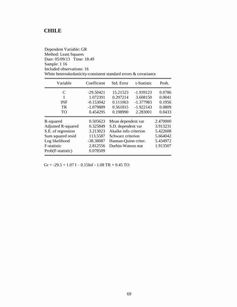
69

CHILE



Date: 05/09/13 Time: 18:49

Sample: 1 16




C -29.50421 15.21523 -1.939123 0.0786

I 1.072391 0.297214 3.608150 0.0041

INF -0.153042 0.111063 -1.377983 0.1956

TR -1.079889 0.561815 -1.922143 0.0809

TO 0.454295 0.198990 2.283001 0.0433








Gr = -29.5 + 1.07 I – 0.15Inf - 1.08 TR + 0.45 TO

70

TURKEY



Date: 05/09/13 Time: 18:53

Sample: 1 16




C -33.13819 26.69405 -1.241407 0.2403

I 1.433039 0.585115 2.449159 0.0323

INF -0.044002 0.046859 -0.939014 0.3679

TR 0.461622 0.727418 0.634603 0.5387

TO -0.016840 0.269659 -0.062448 0.9513








Gr = -33.14 + 1.43 I – 0.04Inf + 0.46 TR – 0.017 TO

71

ISRAEL



Date: 05/09/13 Time: 18:56

Sample: 1 16




C -0.504517 15.38972 -0.032783 0.9744

I 1.294391 0.403395 3.208747 0.0083

INF -0.370158 0.392154 -0.943909 0.3655

TR -0.888522 0.442120 -2.009683 0.0696

TO 0.158842 0.094235 1.685589 0.1200








Gr = -0.50 + 1.29 I – 0.37 Inf – 0.89 TR + 0.16 TO

72

GR = C + I + INF + STOD + TO

CHILE



Date: 05/09/13 Time: 18:45

Sample: 1 16




C -16.61725 23.39498 -0.710291 0.4923

I 0.693696 0.471182 1.472245 0.1690

INF -0.014558 0.608875 -0.023910 0.9814

STOD 0.061699 0.331094 0.186347 0.8556

TO 0.065739 0.220033 0.298769 0.7707








Gr = -16.62 + 0.69 I – 0.01 Inf-c + 0.06 STOD + 0.06 TO

73

MEXICO



Date: 05/09/13 Time: 18:50

Sample: 1 16




C -23.00558 17.92932 -1.283126 0.2258

I 0.549910 0.286102 1.922075 0.0809

INF 0.137287 0.152105 0.902583 0.3861

STOD -0.709465 0.319879 -2.217916 0.0485

TO 0.477052 0.246509 1.935227 0.0791








Gr = -23.005 + 0.55 I + 0.14 Inf – 0.71 STOD + 0.48 TO

74

TURKEY



Date: 05/09/13 Time: 18:53

Sample: 1 16




C -33.55815 15.32904 -2.189188 0.0510

I 2.314080 0.370162 6.251529 0.0001

INF -0.060904 0.026353 -2.311062 0.0412

STOD 0.261930 0.083855 3.123612 0.0097

TO -0.389840 0.360558 -1.081215 0.3027








Gr = -33.56 + 2.31 I – 0.06 Inf + 0.26 STOD – 0.39 TO

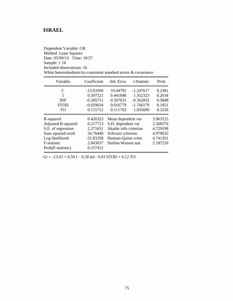
75

ISRAEL



Date: 05/09/13 Time: 18:57

Sample: 1 16




C -13.03500 10.44792 -1.247617 0.2381

I 0.597521 0.441848 1.352323 0.2034

INF -0.285711 0.507631 -0.562832 0.5848

STOD -0.029634 0.016779 -1.766179 0.1051

TO 0.115752 0.111763 1.035690 0.3226








Gr = -13.03 + 0.59 I – 0.28 Inf– 0.03 STOD + 0.12 TO

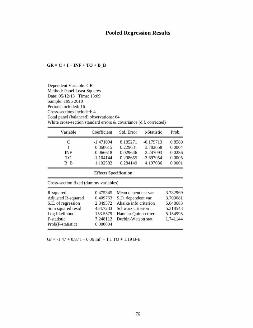
76

Pooled Regression Results

GR = C + I + INF + TO + B_B


Method: Panel Least Squares

Date: 05/12/13 Time: 13:09

Sample: 1995 2010

Periods included: 16

Cross-sections included: 4

Total panel (balanced) observations: 64

White cross-section standard errors & covariance (d.f. corrected)


C -1.471004 8.185271 -0.179713 0.8580

I 0.868615 0.229631 3.782658 0.0004

INF -0.066618 0.029646 -2.247093 0.0286

TO -1.104144 0.298655 -3.697054 0.0005

B_B 1.192582 0.284149 4.197036 0.0001

Effects Specification

Cross-section fixed (dummy variables)








Gr = -1.47 + 0.87 I – 0.06 Inf – 1.1 TO + 1.19 B-B

77

GR = C + I + INF + TR + TO



Date: 05/12/13 Time: 13:11

Sample: 1995 2010






C -15.99026 10.52820 -1.518803 0.1344

I 0.898395 0.228718 3.927965 0.0002

INF_C -0.062199 0.038423 -1.618777 0.1111

TR -0.381708 0.244872 -1.558810 0.1247

TO 0.166379 0.072232 2.303395 0.0250










Gr = -15.99 + 0.9 I – 0.06 Inf – 0.38 TR + 0.16 TO

78

GR = C + I + INF + STOD + TO



Date: 05/12/13 Time: 13:13

Sample: 1995 2010






C -23.97352 9.094258 -2.636116 0.0108

I 0.869805 0.249382 3.487844 0.0010

INF -0.038340 0.029702 -1.290811 0.2021

STOD -0.001187 0.015262 -0.077805 0.9383

TO 0.153127 0.075192 2.036491 0.0464










Gr = -23.97 + 0.87 I – 0.04 Inf – 0.001 STOD + 0.15 TO

The Relationship between Economic Growth, Budget balance ...

Documents

Transcript of The Relationship between Economic Growth, Budget balance ...