The Regional Economics Applications Laboratory (REAL) is · PDF filedirected to Geoffrey J. D....

The Regional Economics Applications Laboratory (REAL) is a cooperative venture between the University of Illinois and the Federal Reserve Bank of Chicago focusing on the development and use of analytical models for urban and regional economic development. The purpose of the Discussion Papers is to circulate intermediate and final results of this research among readers within and outside REAL. The opinions and conclusions expressed in the papers are those of the authors and do not necessarily represent those of the Federal Reserve Bank of Chicago, Federal Reserve Board of Governors or the University of Illinois. All requests and comments should be directed to Geoffrey J. D. Hewings, Director, Regional Economics Applications Laboratory, 607 South Matthews, Urbana, IL, 61801-3671, phone (217) 333-4740, FAX (217) 244-9339. Web page: www.uiuc.edu/unit/real

ON THE SRAFFA-LEONTIEF MODEL by

Michael Sonis and Geoffrey J.D. Hewings

REAL 00-T-2 February, 2000

On the Sraffa-Leontief model.

Michael Sonis Department of Geography, Bar Ilan University, 52900, Ramat-Gan, Israel and Regional Economics Applications Laboratory, University of Illinois, 607 South Mathews, #220, Urbana, Illinois, 61801-3671 email: [email protected] Geoffrey J. D. Hewings Regional Economics Applications Laboratory, University of Illinois, 607 South Mathews, #220, Urbana, Illinois, 61801-3671 email: [email protected]

Abstract. This paper considers the matrix forms of the well-known Sraffa-Leontief income distribution model (1 ) * ( )px r pAx w p I A x= + + − . The equivalence between these matrix forms and the set of simpler models, including the Sraffian condition of linear relations between the rate of profits r and wage rate w* will be explored. Further, the condition that the prices vector p and the commodities vector x are the left hand and the right hand eigenvectors of the matrix A of direct inputs and that these vectors are the fixed points of the Sraffian standard commodities-standard prices matrix will be evaluated. The paper will then explore links between the Sraffa-Leontief system and the multiplier product matrix (MPM) for the matrix A to consider new insights generated through visualization with the help of the artificial economic landscape. Furthermore, the connections between MPM and the Sraffian standard commodities-standard prices matrix and their minimal information properties are proven.

Key words: Sraffa-Leontief income distribution model, Multiplier Product matrix, Sraffian standard commodities-standard prices matrix, minimal information properties. 1. Introduction

The contributions of Sraffa (1960) to the understanding of economic structure have been

significantly advanced in recent years by the interpretative assessments of Steenge (1995, 1997).

In this paper, these interpretations are complemented with some additional modifications that

attempt to simplify the presentation of the Sraffa-Leontief system. In the next section, the

standard Sraffian model is presented and some of the initial modifications are outlined. In

section 3, the concept of the multiplier product matrix (mpm) is introduced but in a modified

form; inside of considering the Leontief inverse matrix, the mpm methodology is applied to the

matrix of direct coefficients to afford a direct link with the Sraffa system. In section 4, the

minimum information properties of the mpm and Sraffian matrix are presented and are shown to

be directly related in sections 5 and 6. Section 7 provides an empirical example from an input-

output table for the Chicago metropolitan region. The paper concludes with some brief summary

remarks and suggestions for further extensions.

mailto:[email protected]

mailto:[email protected]

R E A L On the Sraffa-Leontief Model 2

___________________________________________________________________________________________

2. The Sraffian model.

2.1 Sraffian Prices decomposition matrix Primary model and Commodities decomposition matrix

Dual model.

The simplest and most obvious way to construct the Sraffian income distribution model is as

follows (cf. Pasinetti, 1977): the input-output model is defined in the usual manner:

x Ax f= + (1)

where x is a gross output, A the matrix of input coefficients, and f is the final demand.

Introducing the vector of prices p we obtain:

px pAx pf= + , (2)

where conventionally assumed that the vector of direct labor coefficients

l = pf , (3)

and the total quantity of labor is lx = L=1.

Income distribution theory requires:

*pf rpAx w pf= + (4)

where r is the uniform rate of profits and w* is the wage rate .measured as a share of the national

income, so 0 1.w∗≤ ≤

Substituting (3) and (4) into (2), the Sraffian income distribution model may be obtained:

(1 ) * ( )px r pAx w p I A x= + + − (5)

In matrix form, this model can be presented in the form of a prices decomposition matrix primal

model:

(1 ) * ( )p r pA w p I A= + + − (6)

and in the form of the commodities decomposition matrix dual model:

(1 ) *( )x r Ax w I A x= + + − (7)


___________________________________________________________________________________________

Both matrix models will yield model (5) by post-multiplication of (6) on x and pre-multiplication

of (7) on p.

2.2. Sraffian matrix and decomposition of the matrix A of direct inputs.

Consider a non-negative matrix, A, of direct input coefficients (in the following, it is not

necessary to adopt the usual assumption of decomposability and primitivity of matrix A). From

the theory of non-negative matrices (see, for example, Horn and Johnson, 1985, p. 503), it

follows that there are non-negative eigenvectors (left hand and right hand) p* and x* of A

corresponding to a non-negative eigenvalue µ .

* *, * *p A p Ax xµ µ= = (8)

such that µ is a simple eigenvalue,

It is well known that if the sum of the elements of each column of the matrix of direct inputs is

smaller than 1 and, of course, greater than 0, then the maximal eigenvalue µ is in the interval

0 1µ< < . This follows from the well-known inequality for the spectral radius ( )Aρ of

eigenvalues of positive matrix A (see, for example, Horn and Johnson, 1985, p.346):

( ) min max i i j i i jj j

a A aρ≤ ≤∑ ∑ (9)

The simplicity of µ means that the eigenspaces of all left hand and right hand eigenvectors,

corresponding to µ , are one-dimensional spaces; i.e., each left hand eigenvector is proportional

to p*, and each right hand eigenvector is proportional to x*.

Let us assume (following Steenge, 1995, p. 57) that

p*x*= 1 (10)

and consider the matrix * *S x p= . This matrix will assume a major role in the subsequent

analysis and it will be referred to as the Sraffian matrix with the vector x*, the vector of standard

commodities, and the vector p*, the vector of standard prices. Note that this definition of


___________________________________________________________________________________________

standard commodities is different from the conventional Sraffa definition: Sraffa labeled as

standard commodities the vector of final demand f* generating the gross output x*:

( )* * * 1 *.f x Ax xµ= − = −

For standardization we will assume the constant value of the Sraffian standard commodity

( )* * * * 1pf p f p f µ= = = − (11)

Condition (10) means that these vectors are fixed points of the transformation S:

p*S = p*, Sx* = x* (12)

The conditions (8) imply that

AS SA Sµ= = (13)

Consider further C=I - S. Obviously

2 2= , , 0,

, S S C C CS SCAS SA S AC CAµ

= = == = =

(14)

i.e.,

( )A A S C S CAµ= + = + (15)

Goodwin (1983) and Steenge (1995) used in their considerations the complicated fine structure

(Perronean properties) of the spectrum and spectral decomposition of the matrices with non-

negative components. Alternatively, use will be made here only of the decomposition (15),

where the Perronean eigenvector, corresponding to the larger eigenvalue, and the one-

dimensional eigenspace that splits from the eigenvalues structure. This splitting essentially will

simplify the proofs.

2.3. Sraffa’s linear Wage-Profit trade-off.


___________________________________________________________________________________________

If in the Sraffian model (5), an arbitrary vector of prices p and gross output equal to x*, are

chosen, then substituting gross output x by the eigenvector x* in the Sraffa-Leontief model (5),

using (8) and dividing by px* one obtains:

( ) ( )1 1 * 1r wµ µ= + + − (16)

that implies the Sraffa linear relation between the rate of profits r and the wage rate w* (see

Sraffa, 1960, p.22, see also Pasinetti, 1977, p. 115):

( )11 *r w µµ−= − (17)

Obviously, the maximal rate of profits, corresponding to the case w* = 0 is equal to

max1r µµ−= (18)

The same situation will occurs when the choice is made of an arbitrary gross output x and the

vector of prices p*.

2.4. Equivalence theorems for the Primary Sraffa-Leontief matrix model.

The linear wage-profit trade-off (equations 17 - 18) implies the following statements:

Theorem P1. If ( )α in the Primary Sraffa-Leontief matrix model (6) * 1, w ≠ then ( )β in this

model is equivalent to

1 * (1 *)

w r w

p pAµ

µ− = + −

= (19)

Proof: ( ) ( )α β⇒

The model (6) can be rewritten in the following form:

( )1 * (1 *)w p r w pA− = + − (20)

and, as shown above in section 2.3 implies (17 – 18). The conditions (17 – 18) mean that


___________________________________________________________________________________________

1 * (1 *)w r wµ− = + − (21)

and this implies, after substitution in (20), that:

p pAµ = (22)

( ) ( )β α⇒

Contrarily, if the conditions (19) are true, then multiplying (22) by 1+r - w* and using (21) one

obtains (20), which concludes the proof of equivalence.

2.5. The Steenge equivalence condition.

The following proposition is the reformulation and clarification of the considerations of Steenge,

(1995, pp.63-66). Steenge proved that in Propositions P1 and D1 both conditions in ( )β are

equivalent in the Sraffa model. In his proof, he used the fine structure of the all eigenvalues and

eigenvectors of positive matrices.

Proposition P1. If ( )α in the Primary Sraffa-Leontief matrix model (7) * 1, w ≠ then ( )β this


1 * (1 *)

=w r w

p pSµ− = + −

(23)

Proof: ( ) ( )α β⇒

If condition (22) is true then

( ) ( )pC p I S p pS pA pS p A S pACµ µ µ µ µ µ= − = − = − = − =

This condition means that the vector pC is a left-hand eigenvector for A, and because the

eigenspace corresponding to the simple eigenvalue µ is one-dimensional, then the vector pC is

proportional to p*, i.e., there is a number λ such that *pC pλ= . Using (9) one obtains

*pC p Sλ= . Therefore ( )2 * 0pC pC p S Cλ= = = . Thus,

p pS pC pS= + = (24)


___________________________________________________________________________________________

( ) ( )β α⇒

Conversely, if p = pS, then pC = 0, and pCA = pAC = 0. Therefore

( )pA p S AC pS pµ µ µ= + = =

Thus, (23) is equivalent to (19).

2.6. Equivalence theorems for the Dual Sraffa-Leontief matrix model.

Analogously, the following statement can be proven for the Dual Sraffa-Leontief model (7).

Theorem D1. If ( )α in the Primary Sraffa-Leontief matrix model (7) * 1, w ≠ then ( )β in this


1 * (1 *)

w r w

x Axµ

µ− = + −

= (25)

Proposition D1. (Steenge, 1995). If ( )α in the Dual Sraffa-Leontief matrix model (7) * 1, w ≠ then

( )β this model is equivalent to

1 * (1 *)

w r w

x Sxµ− = + −

= (26)

3. The Multiplier Product Matrix (MPM).

3.1 The definition of MPM.

In this section, a connection between the Sraffa standard commodity system and the multiplier

product matrix will be revealed. The definition of the direct inputs multiplier product matrix

(MPM) is as follows: let ijA a = be a matrix of direct inputs in the input-output system, and let

jm• and im • be the column and row sums of this matrix. Following Chenery and Watanabe

(1958) these are defined as:

1 1

, n n

j ij i iji j

m a m a• •= =

= =∑ ∑ (27)

Let V be the global intensity of the matrix A:


___________________________________________________________________________________________

( ).

1 1

n n

iji j

V V A a= =

= =∑∑ (28)

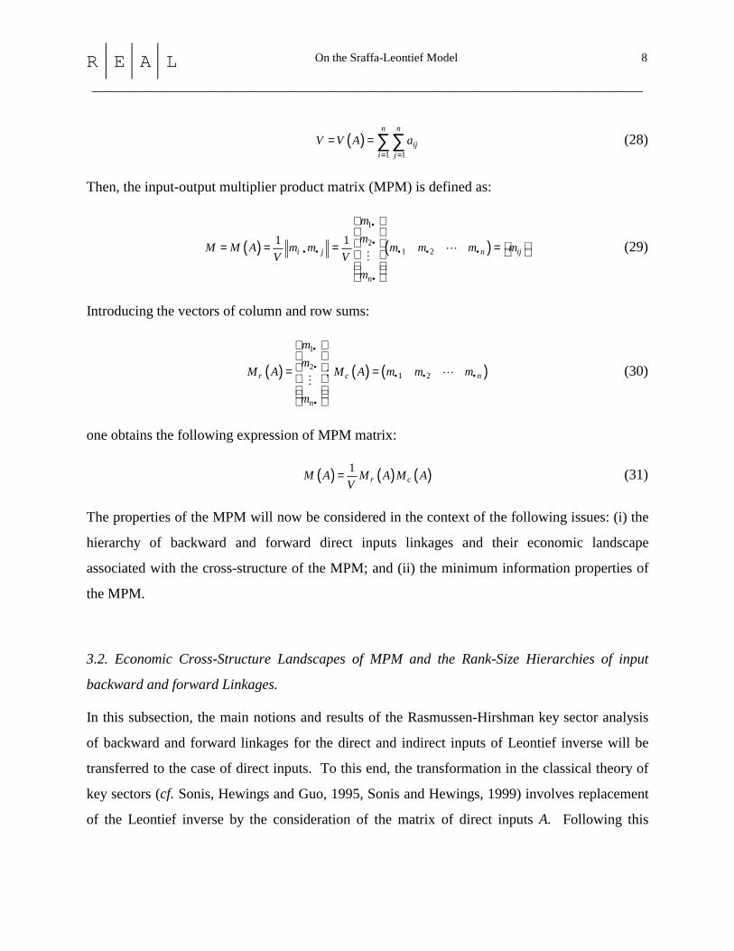
Then, the input-output multiplier product matrix (MPM) is defined as:

( ) ( )1

2 1 2

1 1i j n ij

n

mm

M M A m m m m m mV V

m

•

•• • • • •

•

= = = =

!"

(29)

Introducing the vectors of column and row sums:

( ) ( ) ( )1

21 2; r c n

n

mm

M A M A m m m

m

•

•• • •

•

= =

!"

(30)

one obtains the following expression of MPM matrix:

( ) ( ) ( )1r cM A M A M A

V= (31)

The properties of the MPM will now be considered in the context of the following issues: (i) the

hierarchy of backward and forward direct inputs linkages and their economic landscape

associated with the cross-structure of the MPM; and (ii) the minimum information properties of

the MPM.

3.2. Economic Cross-Structure Landscapes of MPM and the Rank-Size Hierarchies of input

backward and forward Linkages.

In this subsection, the main notions and results of the Rasmussen-Hirshman key sector analysis

of backward and forward linkages for the direct and indirect inputs of Leontief inverse will be

transferred to the case of direct inputs. To this end, the transformation in the classical theory of

key sectors (cf. Sonis, Hewings and Guo, 1995, Sonis and Hewings, 1999) involves replacement

of the Leontief inverse by the consideration of the matrix of direct inputs A. Following this


___________________________________________________________________________________________

analogy, and the ideas of Rasmussen (1956), two types of indices will be defined, drawing on

entries in the matrix A of direct inputs:

1. Power of dispersion of direct inputs for the backward linkages, jDIBL , as follows:

2

1 , 1

2

1 1

1 1 1

n n

j ij iji i j

j j

DIBL an n

m V m Vn nn

= =

• •

= =

= =

∑ ∑ (32)

and

2. The indices of the sensitivity of dispersion of direct inputs for forward linkages, iDIFL , as

follows:

2

1 , 1

2

1 1

1 1 1

n n

i ij ijj i j

i i

DIFL a an n

m V m Vn nn

= =

• •

= =

= =

∑ ∑ (33)

A direct inputs key sector, K, is usually defined as one in which both indices are greater than 1

The definitions of backward and forward linkages provided by (32) and (33) imply that the rank-

size hierarchies (rank-size ordering) of these indices coincide with the rank-size hierarchies of

the column and row sums. It is important to underline, in this connection, that the column and

row sums for MPM are the same as those for the matrix of direct inputs A:

1 1

1 1

1

1

n n

ij i j ij j

n n

ij i j ji i

m m m mV

m m m mV

• • •= =

• • •= =

= =

= =

∑ ∑

∑ ∑ (34)

Thus, the structure of the MPM is essentially connected with the properties of sectoral direct

inputs backward and forward linkages.

The structure of the matrix, M, can be ascertained in the following fashion: consider the largest

column sum, jm• and the largest row sum, im • of the matrix A. Further, the element,


___________________________________________________________________________________________

0 0 0 0

1i j i jm m m

V • •= , is located in the place ( )0 0,i j of the matrix, M. Moreover, all rows of the

matrix, M, are proportional to the 0thi row, and the elements of this row are larger than the

corresponding elements of all other rows. The same property applies to the 0thj column of the

same matrix. Hence, the element located in ( )0 0,i j defines the center of the largest cross within

the matrix, M. If this cross is excluded from M, then the second largest cross can be identified

and so on. Thus, the matrix, M, contains the rank-size sequence of crosses. One can reorganize

the locations of rows and columns of M in such a way that the centers of the corresponding

crosses appear on the main diagonal. In this fashion, the matrix will be reorganized in such a

way that a descending economic landscape will be apparent (see figure 1).

<<insert figures 1, 2 here>>

This rearrangement also reveals the descending rank-size hierarchies of the indices for direct

forward and backward linkages. Inspection of that part of the landscape with indices > 1 (the

criterion for specification of direct inputs key sectors) will enable the identification of the key

sectors (see figure 2). However, it is important to stress that the construction of the economic

landscape for different regions or for the same region at different points in time would create the

possibility for the establishment of taxonomy of these economies. Moreover, the superposition

of the hierarchy of one region on the landscape of another region provides a clear visual

representation of the similarities and differences in the linkage structure of these regions.

It is important to stress, as will be shown in section 6, that the Sraffian standard commodities-

standard prices matrix S coincides with the multiplier product matrix M(S). Hence, the Sraffian

matrix has the same cross-structure defined by rank-size hierarchies of components of vectors of

standard commodities and standard prices (see figure 3).

<<insert figure 3 here>>

4. Minimum Information Properties of the MPM and S.

4.1. Definition of information of the positive matrix.


___________________________________________________________________________________________

Consider all positive matrices, ijψ Ψ = with the property that the row and column multipliers are

equal to those of the matrix A:

, ij i ij jj i

m mψ ψ• •= =∑ ∑ (35)

Obviously, ,

iji j

Vψ =∑ .

We can convert each positive matrixΨ into the two-dimensional probabilistic distribution matrix,

( ),P p i j = with the components:

( ), /ijp i j V= Ψ (36)

Therefore, we can attribute to each positive matrix Ψ the Shannon information (INF):

( ) ( ), ,

, ln , lnij ij

i j i jINF INFP p i j p i j

V Vψ ψ

Ψ = = =∑ ∑ (36)

4.2. Minimum information of MPM and S.

Recall the well-known Shannon information inequality (Shannon and Weaver, 1964, p. 51):

( ) ( ) ( ) ( ) ( ) ( ), , , ,

, ln , , ln , , ln ,i j i j j i j i j

p i j p i j p i j p i j p i j p i j≥ +∑ ∑ ∑ ∑ ∑ (37)

This implies that each positive matrix, Ψ , satisfying the condition (38) may be shown as:

,

2

ln ln ln

ln ln ln ln

ln ln ln

ij ij ij ij ij ij

i j ij j ij ij

ij ij j ij ij ji i

ij ij i j j i

j ji i i ij

i j i j

INFV V V V V V

m mm mV V V V V V V V

m mm m m mmV V V V VV

• •• •

• •• • • ••

Ψ Ψ Ψ Ψ Ψ ΨΨ = ≥ + =

Ψ Ψ Ψ Ψ = + = + =

= + =

∑ ∑ ∑ ∑ ∑

∑ ∑ ∑ ∑ ∑ ∑

∑ ∑ ∑ ∑ 2

2 2 2

ln

ln ln ln .

j ji

j i

i j j i j i ji

ij ij

m mm

VV

m m m m m m mm INFMV VV V V

• ••

• • • • • • ••

+ =

= + = =

∑ ∑

∑ ∑

(38)

Then:


___________________________________________________________________________________________

INF INFMΨ ≥ (39)

and the multiplier product matrix, M, has a minimal information property (Sonis, 1968).

The matrix M may be considered to represent the most homogeneous distribution of the

components of the column and row sums of the matrix A. A further perspective may be offered;

in the case of equal column and row sums, the economic landscape will be a flat, horizontal

plane.

The MPM depends on the column and row sums only and, thus, represents only the aggregate

characteristics of the direct interactions of each sector with the rest of the economy. Thus, MPM

does not take into account the specifics of the pair-wise sectoral interactions between direct

inputs; MPM can be considered as an aggregate representation of some sector equalization

tendency in the economic interaction between sectors. Of course the same property of minimal

information hold for the Sraffian matrix.

5. Properties of column and row multipliers of the product of positive

matrices

In the following, this important property of the multipliers of the product of two positive matrices

will be used. Consider the product 1 2 ijA A A a = = of two matrices 1 21 2, ij ijA a A a = = . Let

1 1

1 1 1 1

1 1

2 2 2 2

1 1

,

,

,

n n

j ij i iji j

n n

j i j i i ji j

n n

j i j i i ji j

m a m a

m a m a

m a m a

• •= =

• •= =

• •= =

= =

= =

= =

∑ ∑

∑ ∑

∑ ∑

(40)

be the column and row multipliers of these matrices. Let

i ji j

V a=∑ be the global intensity of the

matrix A. Further, specify the following vectors of column and row multipliers:


___________________________________________________________________________________________

( ) [ ] ( ) ( )

( ) ( ) ( )

1 1 1 2 2 21 2 1 1 2 2 1 2

1 21 1 1 1 2

2 2 2 1 2

1 2

... ; ... ; ...

; ;: : :

c n c n c n

r r r

n n n

M A m m m M A m m m M A m m m

m mmm m mM A M A M A

m m m

• • • • • • • • •

• ••

• • •

• • •

= = = = = =

(41)

The following formulae can be checked by direct calculations of the components of

corresponding vectors and matrices:

( ) ( )( ) ( )( ) ( ) ( )

1 2

1 2

1 2

;

;c c

r r

c r

M A M A A

M A A M A

V A M A M A

=

=

=

(42)

6. Interconnections between MPM and S.

It is obvious that the standardization condition of vectors x* and p* means that:

( ) ( )*; *c rM S Xp M S Px= = (43)

where X and P are the sums of the components of vectors of standard commodities x* and

standard prices p*

* *; i ii i

X x P p= =∑ ∑ (44)

Thus, the multipliers of the Sraffian matrix S are:

( ) ( )*; *c rM S Xp M S Px= = (45)

and V (A) = PX. Hence, the multiplier product matrix of the Sraffian matrix coincides with the

Sraffian matrix itself:

M(S) = S (46)

Using this property and applying formulae (42) to the condition = = AS SA Sµ one obtains:

( ) ( )*; *c rM A S Xp SM A Pxµ µ= = (46)


___________________________________________________________________________________________

This implies that

( ) ( )* ; *c rM A x X p M A Pµ µ= = (47)

or

( )2

* * PXp M A xVµ= (48)

Further, because the well-known property of the row multipliers:

( )c aM A e v= − (49)

where e = (1,1,..., 1) and vector av is the vector of value added, the conditions (43) and (44)

imply:

( )* *r a ap M A S eS v S Xp v Sµ = = − = −

or

( ) *av S X pµ= − (50)

The standardization (11) help find the exact expression for vector of prices p and vector of

commodities x that are the solutions of the Sraffian models: conditions and p pA x Axµ µ= = means

that p and x are the eigenvectors of A corresponding to the eigenvalue µ . Therefore they are

proportional to p* and x*:

*, *p p x xα β= = .

Introducing them into the standardization condition (11), one obtains 1α β µ= = − , so the

solutions for the Sraffa models are:

( ) ( )1 *; 1 *p p x xµ µ= − = − (51)

Substituting (51) into (5) and (6), the decomposition of prices and commodities in Sraffa-

Leontief models into three parts may be obtained, namely, an intermediate inputs part, an interest

part and a wage part:


___________________________________________________________________________________________

( ) ( ) ( ) ( ) ( )( ) ( ) ( ) ( )( )1 * 1 * 1 * * 1 * ;

1 * 1 * 1 * * 1 *

p p p A r p A w p I A

x x Ax r Ax w I A x

µ µ µ µ

µ µ µ µ

= − = − + − + − −

= − = − + − + − − (52)

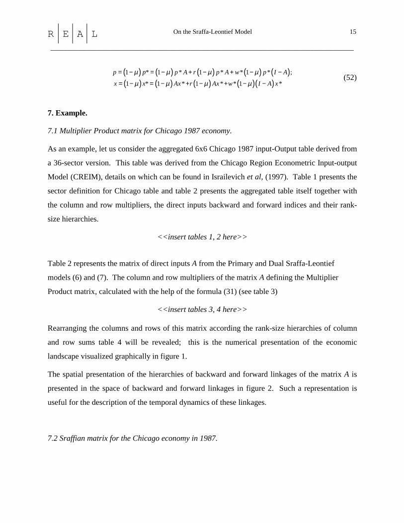
7. Example.

7.1 Multiplier Product matrix for Chicago 1987 economy.

As an example, let us consider the aggregated 6x6 Chicago 1987 input-Output table derived from

a 36-sector version. This table was derived from the Chicago Region Econometric Input-output

Model (CREIM), details on which can be found in Israilevich et al, (1997). Table 1 presents the

sector definition for Chicago table and table 2 presents the aggregated table itself together with

the column and row multipliers, the direct inputs backward and forward indices and their rank-

size hierarchies.

<<insert tables 1, 2 here>>

Table 2 represents the matrix of direct inputs A from the Primary and Dual Sraffa-Leontief

models (6) and (7). The column and row multipliers of the matrix A defining the Multiplier

Product matrix, calculated with the help of the formula (31) (see table 3)

<<insert tables 3, 4 here>> Rearranging the columns and rows of this matrix according the rank-size hierarchies of column

and row sums table 4 will be revealed; this is the numerical presentation of the economic

landscape visualized graphically in figure 1.

The spatial presentation of the hierarchies of backward and forward linkages of the matrix A is

presented in the space of backward and forward linkages in figure 2. Such a representation is

useful for the description of the temporal dynamics of these linkages.

7.2 Sraffian matrix for the Chicago economy in 1987.


___________________________________________________________________________________________

The column sums from table 2 defined, with the help of (10), the interval that includes the

maximal Perronean eigenvalue: 0.2501 0.5261µ< < . The actual value of this maximal eigenvalue

is 0.3367µ = , so the maximal rate of profits in Chicago 1987 economy is

max1 1.97r µµ−= =

The left hand and right hand eigenvectors corresponding to this eigenvalue are: standard prices

eigenvector:

[ ]* 0.7398, 1.464, 0.905, 1.219, 0.89086, 0.9704 , 6.1968p P= =

and standard commodities eigenvector

* * *

0.01920.03410.3568

, 1, 10.18750.07460.3308

x X p x

= = =

The Sraffian matrix of standard commodities, standard prices for Chicago 1987 economy are

presented in table 5:

<<insert table 5 here>> The corresponding economic landscape for this matrix is shown in figure 3

The tables presented above will help us to calculate the decompositions (52) of prices and

commodities in Sraffa-Leontief models into three parts: an intermediate inputs part, an interest

part and a wage part (cf. Steenge, 1997, pp.244-247). This is shown as table A1 in the Appendix.

0.01920.03410.3568

* , 1, * * 10.18750.07460.3308

x X p x

= = =


___________________________________________________________________________________________

8. Conclusions and Further Explorations

This paper has revealed an important connection between the Sraffa-Leontief system and some

new interpretations afforded by the multiplier product matrix. The properties of the latter matrix

offer the potential for comparative analysis across time (for a single economy) or across

economies at one point in time. Further considerations could involve the exploration of an

expansion of the Sraffa-Leontief models by considering the closed system of a Miyazawa type in

which profits and wages are distributed and their impacts on the economy are traced. (cf.

Miyazawa, 1976). In this sense, the work of Trigg (1999), examining a link between Keynes,

Morishima and Miyazawa, provides motivation for the potentially new and innovative insights

that can be gained by exploring connections between modeling systems.

Acknowledgement. Authors would like to thank Professor Albert Steenge for attracting the attention to study of Sraffa models and kind encouragement and help. Chokri Dridi provided the computational expertise to realize the empirical examples. References. Chenery, H.B. and T. Watanabe, (1958) “International comparisons of the structure of production.” Econometrica, 26, 487-521.

Goodwin, R.M. (1983) Essays in Linear Economic Structures. London, Macmillan.

Horn, R.A. and C.A. Johnson, (1985) Matrix Analysis, Cambridge, Cambridge University Press.

Israilevich, P.R., G.J.D Hewings, M. Sonis and G. R. Shindler, (1997) “Forecasting structural change with a regional econometric input-output model.” Journal of Regional Science, 37, 565-590.

Miyazawa, K. (1976) Input-Output Analysis and the Structure of Income Distribution. New York, Springer Verlag.

Pasinetti, L.L. (1977) Lectures on Theory of Production. New York, Columbia University Press.

Rasmussen, P. (1956) Studies in Inter-Sectoral Relationships. Copenhagen, Einar Harks,

Shannon, C.E. & Weaver, W. (1964) The Mathematical Theory of Communications (Urbana, IL, University of Illinois Press).


___________________________________________________________________________________________

Sonis, M. (1968) “Significance of entropy measures of homogeneity for the analysis of population redistributions,” Geographical Problems. Mathematics in Human Geography, 77, 44-63, (in Russian).

Sonis, M. and G.J.D. Hewings, (1999) “Economic landscapes: multiplier product matrix analysis for multiregional input-output systems.” Hitotsubashi Journal of Economics, 40, 59-74.

Sonis, M., G.J.D. Hewings and J-M.Guo, (1995) “Evaluation of economic structure: input-output multiplier product matrix.” Discussion Papers 94-T-12 (revised 1997). Regional Economics Applications Laboratory. University of Illinois, Urbana.

Sraffa, P., (1960) Production of Commodities by Means of Commodities. Cambridge, Cambridge University Press.

Steenge, A.E. (1995) “Sraffa and Goodwin: a unifying framework for standards of value in the income distribution problem.” Journal of Economics, 62, 55-75.

Steenge, A.E. (1997) “The elusive standard commodity: eigenvectors as standards of value”. In A. Simonovits and A. E. Steenge (eds) Prices, Growth and Cycles. Essays in Honor of Andreas Brody. London. Macmillan Press.

Trigg. A.B. (1999) “An interindustry analysis of the relationship between Marx and Keynes,” in G.J.D. Hewings, M. Sonis, M. Madden and Y. Kimura (eds.) Understanding and Interpreting Economic Structure, Heidelberg, Springer-Verlag, 145-153.


___________________________________________________________________________________________

Appendix Table A1: Decomposition of the Sraffian matrix

[ ]

[ ]

0.6633 0.7398,1.464,0.905,1.219,0.89086,0.9704

0.0195 0.0025 0.0101 0.0104 0.0011 0.00120.0273 0.0008 0.0049 0.0245 0.0054 0.01290.0867 0.3109 0

0.6633 0.7398,1.464,0.905,1.219,0.89086,0.9704

=

.1707 0.0889 0.0475 0.08160.0245 0.0381 0.0381 0.1542 0.0600 0.04180.0245 0.0631 0.0385 0.0153 0.0133 0.01500.0676 0.1106 0.0582 0.0776 0.1740 0.1760

+

[ ]

0.0195 0.0025 0.0101 0.0104 0.0011 0.00120.0273 0.0008 0.0049 0.0245 0.0054 0.01290.0867 0.3109 0.1707 0.0889 0.0475 0.0816

0.6633 0.7398,1.464,0.905,1.219,0.89086,0.97040.0245 0.0381

r+ 0.0381 0.1542 0.0600 0.0418

0.0245 0.0631 0.0385 0.0153 0.0133 0.01500.0676 0.1106 0.0582 0.0776 0.1740 0.1760

+

[ ]

0.9805 -0.0025 -0.0101 -0.0104 -0.0011 -0.0012-0.0273 0.9992 -0.0049 -0.0245 -0.0054 -0.0129-0.0867 -0.3109 0.8293 -0.0889 -0.0475 -

*0.6633 0.7398,1.464,0.905,1.219,0.89086,0.9704w+0.0816

;-0.0245 -0.0381 -0.0381 0.8458 -0.0600 -0.0418-0.0245 -0.0631 -0.0385 -0.0153 0.9867 -0.0150-0.0676 -0.1106 -0.0582 -0.0776 -0.1740 0.8240

0.0192 0.0195 0.0025 0.0101 0.0104 0.0011 0.00120.0341 0.0273 0.0008 0.0049 0.0245 0.0054 0.01290.3568 0.0867 0.3109 0.1707 0.0889 0.0475

0.6633 0.66330.18750.07460.3308

=

0.01920.0341

0.0816 0.35680.0245 0.0381 0.0381 0.1542 0.0600 0.0418 0.18750.0245 0.0631 0.0385 0.0153 0.0133 0.0150 0.07460.0676 0.1106 0.0582 0.0776 0.1740 0.1760 0.33

08

+

0.0195 0.0025 0.0101 0.0104 0.0011 0.00120.0273 0.0008 0.0049 0.0245 0.0054 0.01290.0867 0.3109 0.1707 0.0889 0.0475 0.0816

0.66330.0245 0.0381 0.0381 0.1542 0.0600 0.04180.0245

r+

0.01920.03410.35680.1875

0.0631 0.0385 0.0153 0.0133 0.0150 0.07460.0676 0.1106 0.0582 0.0776 0.1740 0.1760 0.3308

+


___________________________________________________________________________________________

0.9805 -0.0025 -0.0101 -0.0104 -0.0011 -0.0012-0.0273 0.9992 -0.0049 -0.0245 -0.0054 -0.0129-0.0867 -0.3109 0.8293 -0.0889 -0.0475 -0.0816

*0.6633-0.0245 -0.0381 -0.0381 0.84

w+

0.01920.03410.3568

58 -0.0600 -0.0418 0.1875-0.0245 -0.0631 -0.0385 -0.0153 0.9867 -0.0150 0.0746-0.0676 -0.1106 -0.0582 -0.0776 -0.1740 0.8240 0.3308


___________________________________________________________________________________________

Table 1. Chicago 1987 Input-Output table sectors definitions

Sectors Aggregate original Description SIC codes

1 Livestock and Other Agricultural Products 01,02 2 Forestry and Fishery; Agricultural Services 07-09

AGM

3 Mining 10-14 CNS 4 Construction 15-17

5 Food and Kindred Products 20 6 Tobacco Manufactures 21 7 Textiles and Apparel 22-23 8 Lumber and wood Products 24 9 Furniture and Fixtures 25

10 Paper and Allied Products 26 11 Printing and Publishing 27 12 Chemicals and Allied Products 28 13 Petroleum Refining and Related Industries 29 14 Rubber and Miscellaneous Plastics Products 30 15 Leather and Leather Products 31 16 Stone, Clay, Glass and Concrete Products 32 17 Primary Metal Industries 33 18 Fabricated Metal products 34 19 Machinery, Except Electrical 35 20 Electrical and Electronic Machinery 36 21 Transportation Equipment 37 22 Scientific Instruments, Photographic and Medical

Goods 38

MNF

23 Miscellaneous Manufacturing Industries 39 24 Transportation and Warehousing 40-42, 44-47 25 Communication 48

TCG

26 Electric, Gas and Sanitary Services 49 WRT 27 Wholesale and Retail Trade 50-57, 59

28 Finance and Insurance 60-64, 67 29 Real Estate and Rental 65, 66 30 Hotels, Personal and Business Services 70-73, 76, 81,

89 31 Eating and Drinking Places 58 32 Automobile Repair and Services 75 33 Amusement and Recreation Services 78,79 34 Health, Educational and Nonprofit Organizations 80, 82-84, 86 35 Federal Government Enterprises

SRV

36 State and Local Government Enterprises


___________________________________________________________________________________________

Table 2. Chicago 1987 direct inputs Input-Output table.

Sectors AGM CNS MNF TCG WRT SRV Row sums

Forward Linkages

DIFL

Rank-Size Hierarchy

of DIFL AGM 0.0195 0.0025 0.0101 0.0104 0.0011 0.0012 0.0447 0.1280 VI CNS 0.0273 0.0008 0.0049 0.0245 0.0054 0.0129 0.0758 0.2168 V MNF 0.0867 0.3109 0.1707 0.0889 0.0475 0.0816 0.7863 2.2497 I TCG 0.0245 0.0381 0.0381 0.1542 0.0600 0.0418 0.3567 1.0205 III WRT 0.0245 0.0631 0.0385 0.0153 0.0133 0.0150 0.1697 0.4856 IV SRV 0.0676 0.1106 0.0582 0.0776 0.1740 0.1760 0.6639 1.8995 II Column

sums 0.2501 0.5261 0.3204 0.3708 0.3011 0.3287

Backward Linkages

DIBL

0.7156 1.5051

0.9166 1.0608

0.8615 0.9403

Rank-Size Hierarchy of

DIBL

VI I IV II V III


___________________________________________________________________________________________

Table 3. Multiplier Product Matrix for Chicago 1987 [direct inputs input-output table]

Sectors

AGM

CNS

MNF

TCG

WRT

SRV

Row

sums

Rank-Size Hierarchy

of row sums

AGM 0.00534 0.01124 0.00684 0.00792 0.00643 0.00702 0.0448 VI CNS 0.00904 0.01902 0.01158 0.01340 0.01088 0.01188 0.0758 V MNF 0.09377 0.19725 0.12013 0.13902 0.11289 0.12324 0.7863 I TCG 0.04254 0.08948 0.05450 0.06307 0.05121 0.05591 0.3567 III WRT 0.02024 0.04257 0.02593 0.03000 0.02436 0.02660 0.1697 IV SRV 0.07917 0.16655 0.10143 0.11738 0.09532 0.10406 0.6639 II Column

sums 0.2501 0.5261 0.3204 0.3708 0.3011 0.3287


Column sums

VI I IV II V III


___________________________________________________________________________________________

Table 4. Economic Landscape for Chicago 1987 Multiplier Product Matrix.

Sectors

CNS

TCG

SRV

MNF

WRT

AGM

Row sums

Rank-Size Hierarchy

of row sums

MNF 0.19725 0.13902 0.12324 0.12013 0.11289 0.09377 0.7863 I SRV 0.16655 0.11738 0.10406 0.10143 0.09532 0.07917 0.6639 II TCG 0.08948 0.06307 0.05591 0.05450 0.05121 0.04254 0.3567 III WRT 0.04257 0.03000 0.02660 0.02593 0.02436 0.02024 0.1697 IV CNS 0.01902 0.01340 0.01188 0.01158 0.01088 0.00904 0.0758 V AGM 0.01124 0.00792 0.00702 0.00684 0.00643 0.00534 0.0448 VI Column

sums 0.5261 0.3708 0.3287 0.3204 0.3011 0.2501


Column sums

I II III IV V VI


___________________________________________________________________________________________

Table 5. Sraffian matrix for Chicago 1987 direct inputs Input-Output table.

Sectors AGM CNS MNF TCG WRT SRV Standard Commodities

x*

Row multipliers

P x*

Rank-Size Hierarchy

of x* AGM 0.014204 0.028104 0.017376 0.023405 0.017253 0.018632 0.0192 0.118979 VI CNS 0.025277 0.049922 0.030861 0.041568 0.030642 0.033091 0.0341 0.211311 V MNF 0.263961 0.522355 0.322904 0.434939 0.32062 0.346239 0.3568 2.211018 I TCG 0.136423 0.270108 0.166973 0.224906 0.165792 0.179039 0.1875 1.14331 III WRT 0.055189 0.109214 0.067513 0.090937 0.067036 0.072392 0.0746 0.462281 IV SRV 0.244726 0.484291 0.299374 0.403245 0.297257 0.321008 0.3308 2.049901 II Column

Multipliers X p*

0.7398 0.464 0.905 1.219 0.8986 0.9704

Standard Prices p*

0.7398 1.464

0.905 1.219

0.8986 0.9704


p*

VI I IV II V III


___________________________________________________________________________________________

CNS TCG SRV MNF WRT AGM

AGMCNS

WRTTCG

SRVMNF

0

0.02

0.04

0.06

0.08

0.1

0.12

0.14

0.16

0.18

0.2

Values of components

Column multipliers

Row multipliers

Figure 1. Economic Landscape for Chicago 1987 input-Output table


___________________________________________________________________________________________

Figure 2. Direct inputs backward and Forward Linkages, Chicago, 1987

0

0.2

0.4

0.6

0.8

1

1.2

1.4

1.6

0 0.5 1 1.5 2 2.5

Forward Linkages

Bac

kwar

d Li

nkag

es

AGM

WRT

CNS

TCG

SRV MNF

Key Sectors

Forward Linkagesoriented sectors

Backward Linkagesoriented sectors

Weaklyoriented sectors


___________________________________________________________________________________________

CN ST CG

SR VMNF

W RTAGM

AG M

CN S

W RT

TC G

SR VMNF

0

0 .1

0.2

0.3

0 .4

0.5

0 .6

V alue s

S ta nda rd P rice s

S ta nda rd C om m odit ies

Figure 3 . Economic Landscape of Sraff ian matrix

The Regional Economics Applications Laboratory (REAL) is · PDF filedirected to Geoffrey J. D....

Documents

Transcript of The Regional Economics Applications Laboratory (REAL) is · PDF filedirected to Geoffrey J. D....