Acta Geodyn. Geomater., Vol. 9, No. 1 (165), 71–77, 2012

THE REALIZATION OF STRONG, STRAY STATIC MAGNETIC FIELDS

Václav ŽEŽULKA* and Pavel STRAKA

Institute of Rock Structure and Mechanics, Academy of Sciences of the Czech Republic, v.v.i., V Holešovičkách 41, 182 09 Prague, Czech Republic *Corresponding author‘s e-mail: zezulka@irsm.cas.cz (Received October 2011, accepted October 2011) ABSTRACT The article introduces the results achieved in the creation of feasible assemblies of NdFeB magnets assembled following analready published design of a practical arrangement of magnets derived from an ideal magnetization pattern, leading to thestrongest possible stray field at a remote point. It presents a method of the implementation of these assembled sets andthe relevant measured dependences of magnetic induction By = f(y) and By = f(x) including their comparison with alreadypublished dependences determined by a simulation. It further presents similar dependences of magnetic induction found in thecase of a trial magnetic circuit with large blocks from NdFeB magnets, and these dependences are compared both withthe mentioned computer-determined dependences and the dependences measured with the corresponding implementedassembly of magnets. KEYWORDS: static magnetic fields, magnetic circuits, permanent NdFeB magnets

deal predominantly with for instance the presentation of analytical expressions for the study of magnetic fields (Ravaud and Lemarquand, 2009), properties of various magnetic configurations for an MRI magnet (Podol’skii, 1998), creation of strong, stray, static magnetic fields (Marble, 2008) or design methodology of single-side magnets (Marble, 2007). Besides the indisputable benefit of computer simulations in the design of any assembly of magnets, however, precisely knowledge and experience acquired in its practical implementation can significantly contribute to deeper knowledge and to decision-making in the further direction of development. The main reason for the implementation of a theoretically designed magnet assembly is the possibility to verify the presented parameters. Nevertheless, it is possible to present as another argument for instance also the seemingly secondary issue, which is the indispensible mastery of the great forces with which particularly NdFeB magnets of materials with high energy products and great dimensions act in the course of assembly on one another and on the surrounding ferromagnetic objects. The determination and verification of a suitable method of the assembly of such magnets is therefore a necessary condition of the implementation of designed assemblies, or circuits, already now. It is clear that with the discovery of a new generation of permanent magnets with an even substantially greater energy product as against the current NdFeB magnets the importance of the methods of their assembly increases even more significantly.

1. INTRODUCTION Magnetization patterns creating a so-called one-

side flux were first described by Mallinson (1973) and then further especially by Halbach (1980). A Halbach array of permanent magnets allows an increase of themagnetic field on one side of this assembly while cancelling this field on the other side. This assemblyhas been implemented in the magnetic systems ofvarious devices, for instance in the case of permanentmagnet brushless machines employing multipoleHalbach magnetized rotors (Zhu and Howe, 2001). Arising from the Halbach cylinder, there are alsopublications dealing with the design and optimization of the assemblies of the permanent magnets for thegeneration of high magnetic fields (Bloch et al.,1998), or comparing the efficiency of various types ofthese assemblies for the creation of uniform fields for MRI devices (Li and Devine, 2005). Other works investigate for example the possibility of the design ofthe Halbach array using numerical optimizationmethods (Choi and Yoo, 2008) or present an algorithm for improving the difference in flux densitybetween a high and a low magnetic-field region in anair gap in a magnetic structure and as an exampleapplied to a two-dimensional concentric Halbach magnet design (Bjork et al., 2011).

A number of works have recently been focusedon applications in NMR and MRI devices and variousassemblies of permanent magnets designed.Sometimes the theoretical design with a simulation is also accompanied by a feasible prototype (Sakellariouet al., 2010), (Wang et al., 2010); other publications

V. Žežulka and P. Straka

72

necessary for the completion of these assemblies were created by cutting from the mentioned blocks witha diamond blade under intensive cooling with water to obtain the required dimensions always in such a way as to preserve the preferential orientation for the desired block-magnetization direction.

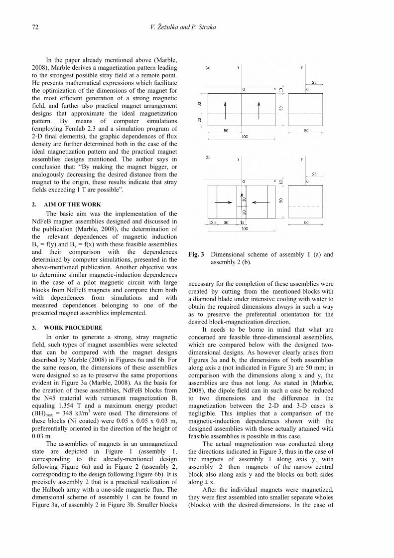
It needs to be borne in mind that what areconcerned are feasible three-dimensional assemblies, which are compared below with the designed two-dimensional designs. As however clearly arises from Figures 3a and b, the dimensions of both assembliesalong axis z (not indicated in Figure 3) are 50 mm; in comparison with the dimensions along x and y, the assemblies are thus not long. As stated in (Marble, 2008), the dipole field can in such a case be reduced to two dimensions and the difference in the magnetization between the 2-D and 3-D cases is negligible. This implies that a comparison of the magnetic-induction dependences shown with the designed assemblies with those actually attained with feasible assemblies is possible in this case.

The actual magnetization was conducted along the directions indicated in Figure 3, thus in the case of the magnets of assembly 1 along axis y, with assembly 2 then magnets of the narrow central block also along axis y and the blocks on both sides along ± x.

After the individual magnets were magnetized, they were first assembled into smaller separate wholes (blocks) with the desired dimensions. In the case of

In the paper already mentioned above (Marble,2008), Marble derives a magnetization pattern leadingto the strongest possible stray field at a remote point.He presents mathematical expressions which facilitatethe optimization of the dimensions of the magnet forthe most efficient generation of a strong magneticfield, and further also practical magnet arrangement designs that approximate the ideal magnetizationpattern. By means of computer simulations(employing Femlab 2.3 and a simulation program of2-D final elements), the graphic dependences of flux density are further determined both in the case of theideal magnetization pattern and the practical magnetassemblies designs mentioned. The author says inconclusion that: “By making the magnet bigger, oranalogously decreasing the desired distance from themagnet to the origin, these results indicate that strayfields exceeding 1 T are possible”.

2. AIM OF THE WORK

The basic aim was the implementation of theNdFeB magnet assemblies designed and discussed inthe publication (Marble, 2008), the determination of the relevant dependences of magnetic inductionBy = f(y) and By = f(x) with these feasible assembliesand their comparison with the dependencesdetermined by computer simulations, presented in theabove-mentioned publication. Another objective wasto determine similar magnetic-induction dependencesin the case of a pilot magnetic circuit with largeblocks from NdFeB magnets and compare them bothwith dependences from simulations and withmeasured dependences belonging to one of thepresented magnet assemblies implemented.

3. WORK PROCEDURE

In order to generate a strong, stray magneticfield, such types of magnet assemblies were selectedthat can be compared with the magnet designsdescribed by Marble (2008) in Figures 6a and 6b. Forthe same reason, the dimensions of these assemblieswere designed so as to preserve the same proportionsevident in Figure 3a (Marble, 2008). As the basis forthe creation of these assemblies, NdFeB blocks from the N45 material with remanent magnetization Brequaling 1.354 T and a maximum energy product(BH)max = 348 kJ/m3 were used. The dimensions ofthese blocks (Ni coated) were 0.05 x 0.05 x 0.03 m,preferentially oriented in the direction of the height of0.03 m.

The assemblies of magnets in an unmagnetizedstate are depicted in Figure 1 (assembly 1, corresponding to the already-mentioned designfollowing Figure 6a) and in Figure 2 (assembly 2, corresponding to the design following Figure 6b). It isprecisely assembly 2 that is a practical realization ofthe Halbach array with a one-side magnetic flux. The dimensional scheme of assembly 1 can be found inFigure 3a, of assembly 2 in Figure 3b. Smaller blocks

Fig. 3 Dimensional scheme of assembly 1 (a) and assembly 2 (b).

THE REALIZATION OF STRONG, STRAY STATIC MAGNETIC FIELDS

73

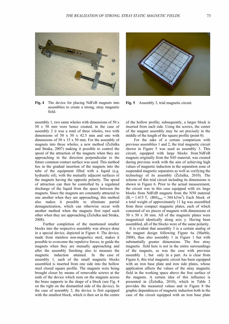
Fig. 5 Assembly 3, trial magnetic circuit. Fig. 4 The device for placing NdFeB magnets intoassemblies to create a strong, stray magneticfield.

of the hollow profile; subsequently, a larger block is inserted from each side. Using the screws, the center of the magnet assembly may be set precisely in the middle of the length of the square profile (point 0).

For the sake of a certain comparison with previous assemblies 1 and 2, the trial magnetic circuit shown in Figure 5 was used as assembly 3. This circuit, equipped with large blocks from NdFeB magnets originally from the N45 material, was created during previous work with the aim of achieving high values of magnetic induction in the separation zone of suspended magnetic separators as well as verifying the technology of its assembly (Žežulka, 2010). The scheme of this trial circuit including its dimensions is shown in Figure 6. Prior to the actual measurement, the circuit was in this case equipped with six large blocks from NdFeB magnets from the N50 material (Br = 1.415 T, (BH)max = 384 kJ/m3). Each block of a total weight of approximately 11 kg was assembled from three compact magnetic plates, each of which consisted of six pieces of magnets with dimensions of 50 x 50 x 30 mm. All of the magnetic plates were magnetized identically along axis y. Having beenassembled, all of the blocks were of the same polarity.

It is evident that assembly 3 is a certain analog of the magnet design following Figure 6a (Marble, 2008), thus also assembly 1 in Figure 1 but with substantially greater dimensions. The free stray magnetic field here is not in the entire surroundings of the magnets, as was the case with previous assembly 1, but only in a part. As is clear from Figure 6, this trial magnetic circuit has been equipped with an iron base plate and iron side plates, whoseapplication affects the values of the stray magnetic field in the working space above the free surface of the magnets. A certain idea of this influence is presented in (Žežulka, 2010), which in Table 2 provides the measured values and in Figure 8 the graphic dependences of magnetic induction both in the case of the circuit equipped with an iron base plate

assembly 1, two same wholes with dimensions of 50 x 50 x 50 mm were hence created, in the case ofassembly 2 it was a total of three wholes, two withdimensions of 50 x 50 x 42.5 mm and one withdimensions of 50 x 15 x 50 mm. For the assembly ofmagnets into these wholes, a new method (Žežulkaand Straka, 2007) making it possible to control thespeed of the attraction of the magnets when they areapproaching in the direction perpendicular to thefuture common contact surface was used. This methodlies in the gradual insertion of the magnets into thetube of the equipment filled with a liquid (e.g.hydraulic oil), with the mutually adjacent surfaces ofthe magnets having the opposite polarity. The speedof attraction can then be controlled by a regulateddischarge of the liquid from the space between themagnets. Since the magnets are constantly attracted toone another when they are approaching, this methodalso makes it possible to eliminate partialdemagnetization, which can otherwise occur withanother method when the magnets first repel eachother when they are approaching (Žežulka and Straka,2008).

Further completion of the mentioned smallerblocks into the respective assembly was always donein a special device, depicted in Figure 4. The device, made from stainless non-magnetics steel, makes it possible to overcome the repulsive forces, to guide themagnets when they are mutually approaching andafter the assembly finishing also to measure themagnetic induction attained. In the case of assembly 1, each of the small magnetic blocksassembled is inserted from one side into the hollowsteel closed square profile. The magnets were beingbrought closer by means of removable screws at theends of the device which rests on the magnets acrossthe brass supports in the shape of a block (see Fig. 4on the right on the dismantled side of the device). Inthe case of assembly 2, the device is first equippedwith the smallest block, which is then set in the centre

V. Žežulka and P. Straka

74

Fig. 6 Dimensional scheme of the trial magneticcircuit (Assembly 3).

-0.1 a.u. to +0.2 a.u. with the values of magnetic induction measured in the corresponding range y (from -10 mm to +20 mm) with a feasible assemblythat:

Assembly 1 – In the entire range, the magnetic-induction values measured with the feasible assemblywere higher than the values provided in the mentionedgraph, determined by a simulation. When appro-aching the surface of the magnets, the difference between the value measured and the value read from the graph at the corresponding point increased. On the surface of the magnets, the maximum magnetic-induction value measured was ca 0.52 T as against the value of ca 0.25 T, read from the graph in (Marble, 2008). It is evident that with the feasible assemblythe increase in magnetic induction when approaching the surface of the magnets is much more significant.

Assembly 2 – Also with the feasible assembly, the magnetic-induction values measured were higher than the values from the given graph, with their difference (determined like with assembly 1) again increasing closer to the surface of the magnets –approximately from zero at point y = 20 mm to ca 0.27 T at point -10 mm (on the surface of the magnets). The maximum actually measured magnetic induction on the surface of the magnets was ca 1.22 T, whereas the value read from the graph in (Marble, 2008) was only ca 0.95 T.

The higher magnetic-induction values measured with both assemblies are very likely to have been attained, because the magnets used had a higher remanence Br = 1.354 T as against remanence Br = 1 T, used in the simulation and in the creation of graphs in (Marble, 2008).

4.2. ASSEMBLIES 1 AND 2, COMPARISON OF

DEPENDENCES By = f(x) AND |B| = f(x) The other dependences measured with assemblies 1

and 2 are shown in Figure 8. Unlike in the graph in Figure 7b in (Marble, 2008), showing dependence |B| = f(x), however, the dependence selected for the measurement on the feasible assemblies 1 and 2 was By = f(x), hence the dependence of only the ypsilon component of vector B on parameter x. The reason were primarily the problems with the precise measurement of the actual size B, because it was shown that a precise measurement of all three components of vector B or directly of their resultant would require an auxiliary device making it possible to set the teslameter probe precisely. Nevertheless, it arose from the measurement that in the range from -20 mm to +20 mm (corresponding to the range x from -0.2 a.u. to +0.2 a.u. in the graph in above-mentioned Figure 7b) both the values Bx and Bz are lower than By(e.g. |Bx| with assembly 1 does not exceed ca 0.07 T),and an idea on the values of dependence |B| = f(x) can thus, while bearing in mind a certain imprecision, be acquired by using dependence By = f(x).

It arises from a comparison of magnetic induction in the graph in Figure 7b with the measured values By in

and only non-magnetic stainless-steel side plates and in the case of the circuit additionally equipped withiron side plates.

4. RESULTS AND DISCUSSION For the measurement of the magnetic-induction

dependence in the case of assemblies 1 and 2, axes ofthe coordinates x and y were selected like in Figure 1 (Marble, 2008), just like the beginning 0 at a distanceof one-tenth of the length of the magnet assemblyfrom the surface of the magnets.

4.1. ASSEMBLIES 1 AND 2, COMPARISON OF

DEPENDENCES By = f(y) The measured dependences By = f(y) of

assemblies 1 and 2 are depicted in Figure 7. Themeasurement was conducted at point x = const = 0,but the maximum values at points y < 10 mm wereachieved with assembly 1 at point x = const = 20 mmand with assembly 2 at point x = const = 5 mm. Thisphenomenon may be caused by the different magneticproperties of the magnets used, the inhomogeneity oftheir composition, or the Ni surface anti-corrosionprotective layer.

It arises from a comparison of the values ofmagnetic induction By provided in the graph inFigure 7a in (Marble, 2008) for y in the range from

THE REALIZATION OF STRONG, STRAY STATIC MAGNETIC FIELDS

75

The influence of the extent of remanent magnetization Br and the application of an iron magnetic circuit can be further specified with reference to the dependence in Figure 8 (Žežulka, 2010), measured on the same assembly 3 but with the N45 material of the magnets with Br = 1.354 T, identical with the material of assemblies 1 and 2. In the same range of 96 mm, the values measured were from ca 0.19 T up to 0.585 T on the surface of the magnets, whereas when this assembly was equipped only with the iron base plate and non-magnetic side plates (i.e. without iron side plates) the values measured in the same range were from ca 0.18 T to 0.535 T.

It is obvious that the values of the magnetic induction By of assembly 3 mainly in the last case approximate the values By = f(y) of assembly 1 (the values from ca 0.17 T to 0.52 T). A further correction of the magnetic induction with assembly 3 can be expected if the iron base plate is replaced with a non-magnetic plate.

4.4. ASSEMBLY 3, COMPARISON OF

DEPENDENCES By = f(x) AND |B| = f(x) Like at point B with assemblies 1 and 2, also in

this case only the values By were measured. The dependences By = f(x) for various constant levels y are given in Figure 10. The range from -0.2 a.u. to +0.2 a.u. in graph 7(b) (squares) (Marble, 2008)corresponds to the range from -64 mm to +64 mm with assembly 3. At the points x = 0 and y = 30 mm (approximately corresponding to the position of the beginning 0 in Figure 3a (Marble, 2008)), the magnetic induction measured was approximately 0.36 T, at the points of ±64 mm it was ca 0.33 T –hence again higher than the corresponding data in above-mentioned graph 7(b) (squares, 0.22–0.23 T). The different shape of the curvatures of the dependences with assembly 3 as against the de-pendences in Figure 7b as well as in Figure 8 in the case of assembly 1 in the corresponding extent of parameter x is then very likely a result of the usage of a ferrous circuit.

5. CONCLUSIONS

The method of the realization of the designsfrom NdFeB magnets whose patterns were presented (including the respective magnetic-induction dependences determined by a simulation) in publication (Marble, 2008) was suggested and verified. The magnetic-induction dependencesmeasured on feasible assemblies were compared with the dependences from this simulation. Furthermore, similar dependences were determined in the case of a trial magnetic circuit with large blocks from NdFeB magnets (assembly 3) and compared both with those calculated and the measured dependences at a feasiblemagnet assembly 1.

The higher measured magnetic-induction values with feasible assemblies when compared with the data

Figure 8 for x in ranges that mutually correspond that: Assembly 1 – The magnetic-induction values with

both dependences compared are almost constant. Withthe feasible assembly, the magnetic-induction values measured in the entire range were again considerablyhigher (approximately 0.36 T) than the values given inthe graph in (Marble, 2008) (ca 0.22–0.23 T).

Assembly 2 – The induction measured at point x = 0with the feasible assembly was slightly higher (0.56 T) than the value given in the above-mentionedgraph (0.53 T). With x increasing both into positiveand negative values with the feasible assembly, however, a far sharper decrease of By values in comparison with the values |B| given is evident. It is likely that this discrepancy is related to the increase ofthe Bx component, whose gradually growing valuesrather considerably affect the size of the resultingabsolute value of magnetic induction.

4.3. ASSEMBLY 3, COMPARISON OF

DEPENDENCES By = f(y) As drawn in Figure 6, the beginning of the

coordinates 0 precisely on the surface of the magnetswas selected for the measurement in this case. Themeasured dependence By = f(y) is shown in Figure. 9. As has been already stated above, this assembly is analogous to the assembly in Figure 6a with the respective graph in Figure 7a (squares) (Marble,2008).

For the sake of a comparison of the measureddependence with this graph, where y is in the rangefrom -0.1 a.u. to +0.2 a.u. (thus a total of 0.3 a.u.), thecorresponding extent y and further ratios for assembly3 were first determined. The ground-plan dimensionsof the assembly of the magnets alone without themagnetic circuit were 320 x 320 mm. With the lengthof the assembly w = 320 mm, the corresponding rangey is 0.3 x 320 = 96 mm. The maximum field can according to the legend for Fig. 3(a) (Marble, 2008)be attained with the ratio of the thickness of themagnet to its length being 0.5, which with the givenlength of the assembly would correspond to the heightof the magnets w/2 = 160 mm. Their actual height washowever only 90 mm and the corresponding ratio ofthe height of the magnets to their length wasapproximately 0.28 and as such is not optimal.Nevertheless, also with this assembly the values Bymeasured in the entire range were again higher than in the graph in above-mentioned Figure 7a (squares) and also the significantly higher increase of magnetic induction when approaching the surface of themagnets, ascertained already with assembly 1, was corroborated. According to this graph, determined by simulation, the magnetic induction in the given rangeincreases from 0.15 T only to 0.25 T on the surfaceof the magnets (approximate values). In the case of assembly 3 with N50 magnets with remanenceBr = 1.415 T, the magnetic induction measured in thecorresponding range was from 0.25 T to almost 0.6 Ton the surface of the magnets.

V. Žežulka and P. Straka

76

Podol’skii, A.: 1998, Development of permanent magnet assembly for MRI devices., IEEE Trans. Magn., 34, no. 1, 248–252.

Ravaud, R. and Lemarquand, G.: 2009, Magnetic field in MRI yokeless devices: analytical approach. Progress in Electromagnetic Research, PIER 94, 327–341.

Sakellariou, D., Hugon, C., Guiga, A., Aubert, G., Cazaux, S. and Hardy, P.: 2010, Permanent magnet assembly producing a strong tilted homogeneous magnetic field: towards magic angle field spinning NMR and MRI. Magnetic Resonance in Chemistry, 48, no. 12, 903–908.

Wang, Z., Yang, W. H., Zhang, X. B., Hu, L. L. and Wang, H. X.: 2010, A design of 1.5 T permanent magnet for MR molecular imaging. IEEE Trans. Appl. Supercond.,20, no. 3, 777–780.

Zhu, Z.Q. and Howe, D.: 2001, Halbach permanent magnet machines and applications: A review. IEE Proc. –Electr. Power Appl., 148, no. 4, 299–308.

Žežulka, V. and Straka, P.: 2007, A new method of assembling large magnetic blocks from permanent NdFeB magnets. Acta Geodyn. Geomater., 4, no. 3 (147), 75–83.

Žežulka, V. and Straka, P.: 2008, Methods of assembling large magnetic blocks from NdFeB magnets with a high value of (BH)max and their influence on the magnetic induction reached in an air gap of a magnetic circuit. IEEE Trans. Magn., 44, no. 4, 485–491.

Žežulka, V.: 2010, Magnetic circuit with large blocks from NdFeB magnets for suspended magnetic separators. Acta Geodyn. Geomater., 7, no. 2 (158), 227–235.

from the graphs in (Marble, 2008) may be explainedby the usage of magnets with a considerably higherremanent magnetization Br, equal to 1.354 T, or1.415 T, than the value Br = 1 T, used in thecalculation. It can also be stated that the values of themeasured magnetic-induction dependences with thesefeasible assemblies correspond to the dependencescalculated – of course while bearing in mind thesubstitute By = f(x) for |B| = f(x), requiring a devicefor the precise measurement of the individualmagnetic-induction components.

The only more significant deviation are thevalues of dependence By = f(y) with both assembly 1 and assembly 3, where the increase in the measuredmagnetic induction is substantially greater closer tothe surface of the magnets in comparison with thecalculated data published.

The magnetic-induction values measured withassembly 3 corroborate the generally known fact thatusing a suitable type of a ferrous magnetic circuit canin a certain area further increase the magneticinduction of a stray magnetic field. ACKNOWLEDGEMENTS

This work was supported by the Academy ofSciences of the Czech Republic as a part of theInstitute Research Plan, Identification Code AVOZ30460519. REFERENCES Bjork, R., Bahl, C.R.H., Smith, A. and Pryds, N.: 2011,

Improving magnet designs with high and low fieldregions. IEEE Trans. Magn., 47, no. 6, 1687–1692.

Bloch, F., Cugat, O., Meunier, G. and Toussaint, J. C.: 1998,Innovating approaches to the generation of intensemagnetic fields: Design and optimization of a 4 Teslapermanent magnet. IEEE Trans. Magn., 34, no. 5,2465–2468.

Halbach, K.: 1980, Design of permanent multipole magnetswith oriented rare earth cobalt material. Nucl. Instrum.Methods, 169, issue 1, 1–10.

Choi, J. and Yoo, J.: 2008, Design of a Halbach magnetarray based on optimization techniques. IEEE Trans.Magn., 44, no. 10, 2361-2366.

Li, C. and Devine, M.: 2005, Efficiency of permanentmagnet assemblies for MRI devices. IEEE Trans.Magn., 41, no. 10, 3835–3837.

Mallinson, J.C.: 1973 “One-side fluxes – A magneticcuriosity?,” IEEE Trans. Magn., 9, no. 4, 678–682.

Marble, A. E., Mastikhin, I. V., Colpitts B. G. and Balcom,B. J.: 2007, Designing static fields for unilateralmagnetic resonance by a scalar potential approach.IEEE Trans. Magn., 43, no. 5, 1903–1911.

Marble, A. E.: 2008, Strong, stray static magnetic fields.IEEE Trans. Magn., 44, no. 5, 576-580.

V. Žežulka and P. Straka: THE REALIZATION OF STRONG, STRAY STATIC MAGNETIC ….

Fig. 2 Assembly 2. Fig. 1 Assembly 1.

-0.1

0

0.1

0.2

0.3

0.4

0.5

0.6

-40 -20 0 20 40

x [mm]

B y [T

]

Assembly 1, By = f(x), atlevel y = const = 0Assembly 2, By = f(x), atlevel y = const = 0

0

0.2

0.4

0.6

0.8

1

1.2

1.4

-20 -10 0 10 20 30 40y [mm]

B y [T

]

Assembly 1, By = f(y) at point x = const = 0

Assembly 1, By = f(y) at point x = const = 20

Assembly 2, By = f(y) at point x = const = 0

Assembly 2, By = f(y) at point x = const = 5

Fig. 8 Dependence By = f(x) for assemblies 1 and 2.

Fig. 7 Dependence By = f(y) for assemblies 1 and 2.

0

0.05

0.1

0.15

0.2

0.25

0.3

0.35

0.4

-200 -100 0 100 200x [mm]

B y [T

]

Assembly 3, By = f(x), at level y = const = 30 mmditto, at level y = const = 60 mmditto, at level y = const = 120 mmditto, at level y = const = 150 mmditto, at level y = const = 200 mm

0

0.1

0.2

0.3

0.4

0.5

0.6

0.7

0 100 200 300 400 500y [mm]

B y [

T]

Assembly 3, By = f(y) at pointx = const = 0

Fig. 10 Dependence By = f(x) for assembly 3.

Fig. 9 Dependence By = f(y) for assembly 3.