The Rational Voter Paradox Revisited

The Rational Voter Paradox RevisitedAuthor(s): Emory PetersSource: Public Choice, Vol. 97, No. 1/2 (Oct., 1998), pp. 179-195Published by: SpringerStable URL: http://www.jstor.org/stable/30024420 .

Accessed: 16/06/2014 00:33

Your use of the JSTOR archive indicates your acceptance of the Terms & Conditions of Use, available at .http://www.jstor.org/page/info/about/policies/terms.jsp

.JSTOR is a not-for-profit service that helps scholars, researchers, and students discover, use, and build upon a wide range ofcontent in a trusted digital archive. We use information technology and tools to increase productivity and facilitate new formsof scholarship. For more information about JSTOR, please contact [email protected].

.

Springer is collaborating with JSTOR to digitize, preserve and extend access to Public Choice.

http://www.jstor.org

This content downloaded from 195.34.78.81 on Mon, 16 Jun 2014 00:33:35 AMAll use subject to JSTOR Terms and Conditions

http://www.jstor.org/action/showPublisher?publisherCode=springer

http://www.jstor.org/stable/30024420?origin=JSTOR-pdf

http://www.jstor.org/page/info/about/policies/terms.jsp


Public Choice 97: 179-195, 1998. 179

© 1998 Kluwer Academic Publishers. Printed in the Netherlands.

The rational voter paradox revisited

EMORY PETERS The Peterson Companies, Senior-Vice President, 12500 Fair Lakes Circle, Fairfax, VA 22033-3804, U.S.A.

Accepted 18 November 1997

Abstract. The rational voter paradox rests on two fundamental assumptions. First, that voters are risk neutral. Second, that voters make decisive vote computations. The implications of maximizing the expected utility of wealth rather than the utility of expected wealth are

explored. The validity of decisive vote computations are examined through concepts of weak and strict in the limit free rider assumptions. The paper proposes a margin of victory model of voting behavior based on information levels and the political division of labor.

1. Introduction

The investment motive is rich with implications, and the consumption motive less well endowed, so we should see how far we can carry the former before we add the latter (Stigler, 1972: 106).'

The rational voter paradox remains a central problem of the rational choice approach to politics (Green and Shapiro, 1994: especially Ch. 4). If rational self-interest, rather than concern for the public good, is the real driving motivation behind political action, why do people vote? The probability of a voter deciding an election is essentially infinitesimal (Owen and Groofman, 1984).2 Therefore, the expected value of voting will almost always be less than the cost to vote. The reasoning proceeds that if the voter will not decide the election, it is senseless to vote or expend the cost to vote. Downs (1957) conjectured that the present value of democracy must be the ultimate motivation for voting. If voters did not show up at the polls, democracy would cease to function. The equation is thus presented in the literature as:

PB + D > C



180

P = the probability of the voter deciding the election B = the net benefit to the voter between the two candidates C = the cost to vote

D = the present value of democracy (Mueller, 1993).3

A rational choice model might properly consider the long-term benefit of democracy. However, that value should be subject to the same probability of occurrence as the short-term benefit. Though the present value of democracy is a "good", so is the net benefit to the voter. Either good is desirable but they are still subject to the probability of producing the outcome. The voters' chance of preserving democracy by voting is still essentially infinitesimal and the same free rider problem applies. Thus the equation should be rewritten as P(B + D) > C, with D inside the brackets. The magnitude inside the brackets would be larger but still subject to the essentially infinitesimal probability of procuring the outcome (deciding the election). In order to pursue the investment motive more directly, I will present a model that includes only B, and deals only with the relation of PB and C.4

Downs original model was considerably less formal than those which have followed. A popular formal model sets out the computation as follows (see note 2):

P = 3e-2(N-1)(p-.5)^2/2n(N-1)

where

P = the probability the voter decides the election

N = the total number of expected voters

p = the probability that the other voters will vote with the voter.

Currently, approximately 100,000,000 voters turn out at Presidential elections so even if p = .5,

P = 3e-2(N-1)(0)^2/n(N-1)

= 3(1)/99,999,999

= 1.197/99,999,999

= .00012.

If p = .5, then e raised to the power 0 equals I and we get the highest possible value for this function. As discussed in note two, the value declines as p diverges in either direction from .5.

The paradox results from two conditions which on the surface appear indisputable, but which upon careful examination will not hold up. First,



181

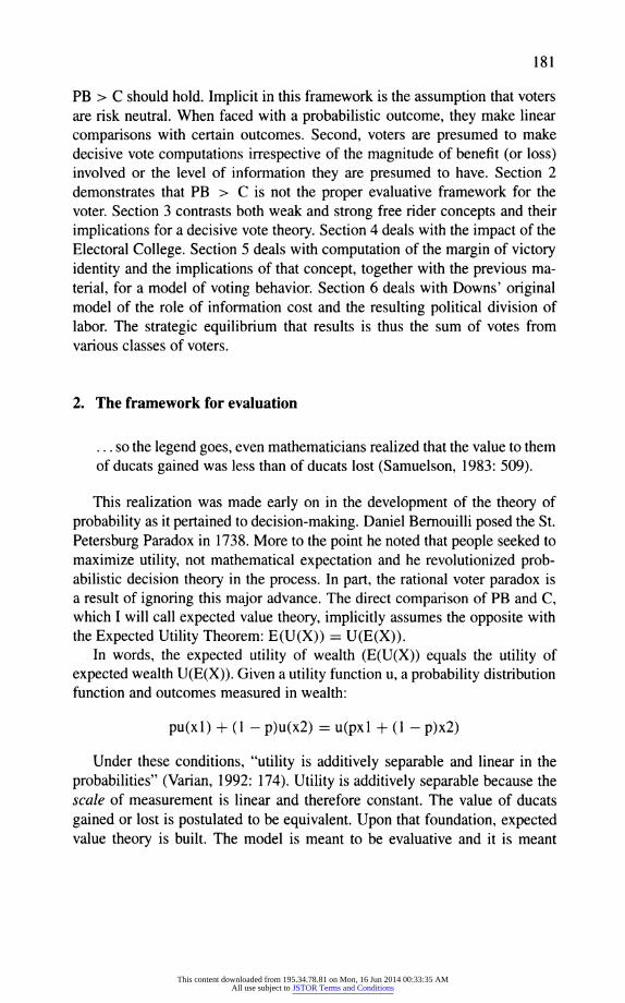
PB > C should hold. Implicit in this framework is the assumption that voters are risk neutral. When faced with a probabilistic outcome, they make linear comparisons with certain outcomes. Second, voters are presumed to make decisive vote computations irrespective of the magnitude of benefit (or loss) involved or the level of information they are presumed to have. Section 2 demonstrates that PB > C is not the proper evaluative framework for the voter. Section 3 contrasts both weak and strong free rider concepts and their implications for a decisive vote theory. Section 4 deals with the impact of the Electoral College. Section 5 deals with computation of the margin of victory identity and the implications of that concept, together with the previous ma- terial, for a model of voting behavior. Section 6 deals with Downs' original model of the role of information cost and the resulting political division of labor. The strategic equilibrium that results is thus the sum of votes from various classes of voters.

2. The framework for evaluation

... so the legend goes, even mathematicians realized that the value to them of ducats gained was less than of ducats lost (Samuelson, 1983: 509).

This realization was made early on in the development of the theory of probability as it pertained to decision-making. Daniel Bernouilli posed the St. Petersburg Paradox in 1738. More to the point he noted that people seeked to maximize utility, not mathematical expectation and he revolutionized probabilistic decision theory in the process. In part, the rational voter paradox is a result of ignoring this major advance. The direct comparison of PB and C, which I will call expected value theory, implicitly assumes the opposite with the Expected Utility Theorem: E(U(X)) = U(E(X)).

In words, the expected utility of wealth (E(U(X)) equals the utility of expected wealth U(E(X)). Given a utility function u, a probability distribution function and outcomes measured in wealth:

pu(xl) + (1 - p)u(x2) = u(pxl + (1 - p)x2)

Under these conditions, "utility is additively separable and linear in the probabilities" (Varian, 1992: 174). Utility is additively separable because the scale of measurement is linear and therefore constant. The value of ducats gained or lost is postulated to be equivalent. Upon that foundation, expected value theory is built. The model is meant to be evaluative and it is meant



182

to have both predictive and prescriptive implications. Expected value theory predicts that people will accept fair gambles (irrespective of the amount wagered), will not purchase insurance and in this application, not vote. A rational individual will evaluate uncertain outcomes according to their expected value (mathematical expectation) as follows:

E(V) = A Indifferent E(V) < A Prefer A E(V) > A Prefer E(V) A = a money outcome

In general form, the equation is:

E(V) = f(x)g(v)

where f(x) = a probability density function and g(v) = a payoff function. The payoff function assigns a money value to each point in the sample

space and is discrete or continuous depending on the nature of the probability density function.

Economists have captured the essence of Bernoullis' observation with the concept of diminishing marginal utility of wealth. Mathematically, this concept is represented very generally as a utility of wealth function u(w) such that u'(w) > 0 and u"(w) < 0. In stark contrast to the Expected Utility Theory is Jensens' Inequality which holds under conditions of diminishing marginal utility of wealth (or any strictly concave function): E(U(X)) < U(E(X)).

Jensens' Inequality predicts that people will avoid fair gambles, purchase insurance and maybe they will vote. Using Jensens Inequality, let us model a simple "fair game" such as a coin toss. Let x = the amount wagered and w* = current wealth with p = the probability of winning (losing) = .5.

.5u(w* - x) + .5u(w* + x) < u(.5(w* - x) + .5(w* + x))

.5u(w* - x) + .5u(w* + x) < u(.5w* - .5x + .5w* + .5x)

.5u(w* - x) + .5u(w* + x) < u(w*)

Some 0 > 0 must exist for all x such that: .5u(w*-x)+.5(w*+x) = u(w*-8) Denote the function F = .5u(w* - x) + .5u(w* + x) - u(w* - 0) = 0

and 0 is implicitly a function of x. The rate of change of F with respect to 0 is:

8F/8- = -u'(w* - 0)dw/d0 = u'(w* - 0) and since u'(w) > 0, &F/80 # 0 and therefore, by the implicit function rule of differentiation, the change in 0 with respect to x is -Fx/Fo



183

Fx = .5u'(w* - x)(-1) + .5u'(w* + x)(1) = -.5u'(w* - x) + .5u'(w* + x)

Therefore

.5(u'(w* - x) - u'(w* + x)) 80/8x =

u'(w* - 0)

Since u'(w) > 0, u'(w* -0) > 0, and since u"(w) < 0, u'(w* -x) > u'(w*+ x) and a0/ax > 0. Thus 0 is strictly increasing in x. The sign of the second derivative indicates whether 0 is increasing at a decreasing or increasing rate.

U'(w* - 9)(.5(u"l(w* - x)(-l) - u"(w* + x)(l)) - .5(u'(w* - x) - u'(w* + x))x0 a28/ax2 =

(u'(w* - 0))2

= -.5(u"(w* - x) + u"(w* + x))

u'(w* - 0)

Since u"(w) < 0, -.5(u"(w* - x) + u"(w* + x)) > 0 as is u'(w* - 0) and therefore, a20/aX2 > 0. Thus, 0 is strictly increasing in x at an increasing rate. To test this proposition it is only necessary to observe behavior. It is really quite remarkable how quickly people will drop out as you offer to toss a coin for increasing amounts ($1, $5, $10 etc.). It is quite clear that 0 is increasing at an increasing rate. This example was given because this function is quite easy to sign unambiguously, and rather easy to see intuitively that 0 is increasing at an increasing rate.

Now let us move to a model which allows us to examine how we evaluate a foregone opportunity. Economists consider cost as the value of the next best alternative foregone when a choice is made. This would certainly include uncertain outcomes. Let: b = opportunity cost of not voting = net benefit between the candidates, then by Jensens' Inequality:

pu(w* - b) + (1 - p)u(w* - 0) < u(p(w* - b) + (1 - p)(w* - 0)) < u(pw* - pb + w* - pw*) < u(w* - bp)

there must be some 3 > 1, so that:

pu(w* - b) + (1 - p)u(w*) = u(w* - Spb)

It is useful to understand S as a multiple of expected loss. From the same functional relationships we can extract more information about S than if it was represented as another magnitude subtracted as in w* - S - pb.5 To



184

u(W)

u(W') u(W*-p'b')

u(W*-ap'b*) E

D

Tr

- 6

p*u(W*-b*)+(l-p*')u(W")

u(W)-b*)

0 W*-b* W. -p*b" W*-p*b* W" W

Figure 1.

gain some intuitive insight refer to Figure 1. The utility of wealth is represented on the y axis and wealth itself on the x axis. Point A is the coordinate (u(w*), w*). The utility of current wealth, w*, can be read off the y axis for w*, read of the x axis. For a given potential loss, b*, the coordinates are (u(w* - b*), (w* - b*)). This is represented at point B. The concave line indicates the utility of wealth function. The chord connecting A and B is the function pu(w* - b) + (1 - p)u(w*) with b held constant, allowing only p to vary. I have illustrated the affect of a given p* on that chord at point C. The coordinates of that point are:

([p*u(w* - b*) + (1 - p*)u(w*), [w* - p*b*]). At point D we see that u(w* - p*b*) is indeed greater than p*u(w* - b) + (1 - p*)u(w*). Finally at point E we have the utility of wealth at u(w* - Sp*b*) which is equivalent to the utility at p*u(w*b) + (1 - p*)u(w*). The slope of the chord is AUL/AWL = [u(w*) - u(w*b*)]/[w* - (w* - b*)] = [u(w*) - u(w* - b*)]/b. It is the rate of change in utility over the entire range of the loss. The slope of AUL/AWL is clearly higher than the slope of the chord that connects point D and point A. It is also greater than the slope of the chord that connects point E and point A.



185

u(W)j

C'

b*p'

C.

b'p"

0 W-8b*p" Wl-b*p" W-8 p'b* W*-p'b* wV* W

Figure 2.

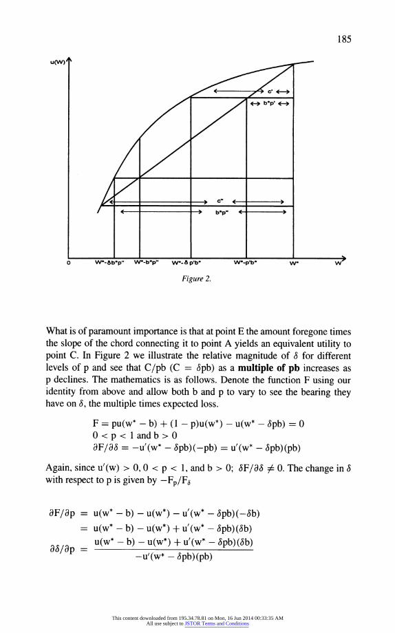
What is of paramount importance is that at point E the amount foregone times the slope of the chord connecting it to point A yields an equivalent utility to point C. In Figure 2 we illustrate the relative magnitude of 3 for different levels of p and see that C/pb (C = Spb) as a multiple of pb increases as p declines. The mathematics is as follows. Denote the function F using our identity from above and allow both b and p to vary to see the bearing they have on 3, the multiple times expected loss.

F = pu(w* - b) + (1 - p)u(w*) - u(w* - Spb) = 0 O<p< 1andb>0 aF/la = -u'(w* - Spb)(-pb) = u'(w* - Spb)(pb)

Again, since u'(w) > 0, 0 < p < 1, and b > 0; 8F/S # 0. The change in 8 with respect to p is given by -Fp/F3

aF/ap = u(w* - b) - u(w*) - u'(w* - 8pb)(-Sb) = u(w* - b) - u(w*) + u'(w* - 8pb)(8b)

u(w* - b) - u(w*) + u'(w* - Spb)(8b) -u'(w* - Spb)(pb)



186

= u(w*) - u(w* - b) - u'(w* - Spb)(3b) u'(w* - Spb)(pb)

(u(w*) - u(w* - b) - u'(w* - Spb)(Sb)) = (1/pb) u'(w* - Spb)

((u(w*) - u(w* - b))/b - u'(w* - Spb)(3)) = (1/p) u'(w* - Spb)

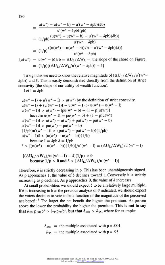
[u(w*) - u(w* - b)]/b = AUL/AWL = the slope of the chord on Figure = (1/p)[(AUL/AWL/u'(w* - Spb)) - 3]

To sign this we need to know the relative magnitude of (AUL/AWL/U'(w*- Spb)) and S. This is easily demonstrated directly from the definition of strict

concavity (the shape of our utility of wealth function). Let I = Spb

u(w* - I) + u'(w* - I) > u(w*) by the definition of strict concavity u(w* - I) + (u'(w* - I)I - u(w* - I) > u(w*) - u(w* - I) u'(w* - I)I > u(w*) - [pu(w* - b) + (1 - p)u(w*)]

because u(w* - I) = pu(w* - b) + (1 - p)u(w*) u'(w* - I)I > u(w*) - u(w*) + pu(w*) - pu(w* - b) u'(w* - I)I > pu(w*) - pu(w* - b) (1/pb)u'(w* - I)I > (pu(w*) - pu(w* - b))(1/pb) u(w* - I)8 > (u(w*) - u(w* - b))(1/b)

because I = Spb 3 = I/pb 6 > [(u(w*) - u(w* - b))(1/b)]/u'(w* - I) = (AUL/AWL)/u'(w* - I)

[(AUL/AWL)/U/(W* - I) - S](l/p) < 0 because 1/p > 0 and S > [AUL/AWL)/U'(W* - I)]

Therefore, S is strictly decreasing in p. This has been unambiguously signed. As p approaches 1, the value of S declines toward 1. Conversely it is strictly increasing as p declines. As p approaches 0, the value of S increases.

At small probabilities we should expect S to be a relatively large multiple. If 0 is increasing in b as the previous analysis of 0 indicated, we should expect the voters decision to vote to be a function of the magnitude of the perceived net benefit.6 The larger the net benefit the higher the premium. As proven above the lower the probability the higher the premium. This is not to say that S.oolP.oolb* > .9P.95.b*, but that S.oo0 > 8.95, where for example:

S.oo1 = the multiple associated with p = .001

8.95 = the multiple associated with p = .95



187

The evaluative framework for the voter is u(w* - Spb) > u(w* - c) where c = the cost to vote. Since u'(w) > 0, it is sufficient that Spb > c or pb > c/S. As 3 increases, the magnitude of c/3 declines. For example: if the combined effect of p and b indicated a subjective premium multiple of, say, 30 where

p = .00012 and b = 10,000, then the evaluation of the cost to vote and the foregone opportunity cost would be:

(.00012)(10, 000)(30) = 36 > c

You will note that I have used .00012 as the value of p. I will deal with the appropriate values of p in subsequent sections. But at least under these circumstances it no longer seems impossible that a voter would vote. Without the multiple we would have the condition 1.2 > c. The question of the magnitude of the multiple seems to be an empirical one that is quite difficult to measure. However, I would be quite surprised if title insurance purchased to insure over the owners equity in a home purchase, for example, didn't yield similar (or greater) multiples. Empirical tests to establish the magnitude of the multiples for circumstances with at least similar amounts at risk and at similar probabilities would be crude. They would confirm at least the concept of the willingness of consumers (voters) to pay multiples of expected value to avoid random losses, especially for events with a very small likelihood of occurrence and for a sufficiently large potential loss. Because of competition, the multiples paid for insurance in the marketplace will not indicate the full extent of voter willingness to pay multiples. In the case of an insurance market a considerable consumer surplus may hide the true multiple which would be paid in the absence of competition. It is important to distinguish the difference here as Figure 3 indicates. There is no mechanism which produces a supply curve that provides a consumer surplus. The dotted line for the supply curve indicates that no such mechanism exists in the political marketplace.

3. The free rider effect and the decisive vote theory

The infinitesimal probabilities computed from the formal models result from the decisive vote theory. The usual application of expected value theory would not even reference the large P used in the formal model. If the voter perceives that p = .5 then .56b > c implies Sb > 2c. Even if p were less than .5, say .25, then .256b > c implies Sb > 4c is all that is required to induce the voter to vote. Without the free rider effect there is no rational voter paradox at all.

PB - C C> 0

where



188

COST

(6pb)

Consumer Surplus /

Insurance 0

Figure 3.

P = the percentage of the total population voting with the voter B = the net benefit between the candidates C = the cost to vote

A landslide is 60% against! Very few voters would have benefits from voting which would not justify voting. This model would be consistent with expected value theory and it is consistent with the kind of probabilistic computations the voter makes everywhere else in his life. This approach ignores the free rider issue which we can call the weak in the limit free rider assumption: The voter will expend cfor a sufficient Spb regardless of the number of voters that will decide the election for or against him. But if Spb-c is sufficiently small or if the number of voters that would decide the election for or against him was sufficiently large, would not voters be willing to forego the potential benefit of voting in favor of accepting the benefit of free riding?

From the other direction, the assumption that the voter computes the probability of the decisive vote instead is a radical application of the free rider concept. Let us formalize this assumption and define it as the strict in the limit free rider assumption which states: The voter will not expend c regardless of the magnitude of Spb, if one other voter will decide the election either for or against him. Would the voter be willing to expend c if he thought only one other voter might decide the election? Or two? Or ten thousand? Only in a world of perfect certainty. The free rider effect has been demonstrated to provide under provision of a particular public good; not no provision whatso-



189

ever. By similar reasoning, we would conclude that no one would contribute to public television.

It would also seem that the magnitude of 3pb-c would have an impact on the voters' willingness to forego the potential benefit of voting in favor of accepting the benefit of free riding. Perhaps we should modify the formal model:

P = 3e-2(N-1-x)(p-.5)^2

where

x = f(Spb - c)

The subject voter should be willing to risk x voters, who might otherwise decide the election, before deciding to free ride. Thus we have seen that the strict in the limit free rider assumption drives the infinitesimal P and subsequent large B requirements of the formal model.7 Working from either direction we end up in a similar position of believing that there is some para- metric adjustment to the decisive vote theory; depending on the magnitude of Spb and the number of voters who will otherwise decide the election.

4. The Electoral College

Presidential elections are not decided by direct election by individual voters. The Electoral College has its roots in Federalism. The small states were in- duced to join the Union through Constitutional assurances that the legislature would be bicameral with the House based on population and the Senate based on the number of states. The President would be elected by an Electoral College which was a compromise. Votes in the Electoral College are computed by giving each state the number of votes that it has in the House and the Senate combined. Subsequently, the District of Columbia has been given three Electoral votes. There are, then, a total of 538 votes.

House 435 Senate 100

D.C. 3 538

The Constitution leaves the matter of how the states vote their electoral votes entirely to the states themselves. Over the years each and every state has



190

decided to vote their votes as a block. This practice maximizes the political leverage of the state in Presidential elections. Thus each state has adopted a winner take all approach to casting their electoral college votes at the state constitutional decision-making level. If candidate A gets 51% of the votes in the state, he gets 100% of the electoral vote (Hardaway, 1994). What consequences does this institutional setting have for voting behavior?

First, the actual outcome of the election (the candidate selected) in a political party system is not the only consequence of the election. A pre-election bargaining process may distribute differential incentives based on the lever-

age that each state brings to the election and the certainty with which the state can be "delivered". These incentives form the benefits which accrue to active participants in the political division of labor. Though Downs (1957) is remembered for his spatial model of politics, An economic theory of democracy is properly understood as a study in how information cost produces a

political division of labor and affects the behavior of parties and voters. Second, the voter is not competing with 100,000,000 voters to influence

the outcome of the election. He is competing with only those other voters in his state. The free rider effect is less prevalent. If his candidate wins at the state level, he gets the benefit of the entire electoral vote for his candidate. In terms of impact on the outcome of the election he receives two times the electoral college votes of his state. Once for winning and once for not losing.

The model for an electoral college computation should be:

P(A21A2 = P(A2)xP(AI)

where P(AI) = the probability of deciding the state election given x number of voters the voter will bear before deciding to free ride given the magnitude of

Spb-c and P(A2) = the probability the state will decide the election Pr(270 -

2E < X < 270) where E = the number of electoral votes. Discussions in the previous literature have always considered the proba-

bility problem to be a random, independent probability even at the Electoral

College level (Owen and Grofman, 1984, and another very interesting article

by Barzel and Silberberg, 1973). I am inclined to agree that, in California, where 15,000,000 voters arrive at the polls, that the individual voter's vote counts as one random event. This is still possibly the case in Vermont where less than 300,000 turn out.9 But at the electoral college level I just cannot

agree it is just another random, independent event. There are only 538 total votes. A total of 270 wins the election. A swing in California, for example, constitutes 54 x 2 = 108 electoral votes. This is not a random, independent event. And the voter is voting to control 2 x E due to the winner take all nature of the election. This is not a random, independent event but a strategic one. This factor alone would account for a great deal of the discrepancy between



191

the number of voters who show up and the number we would expect in a random probabilistic game.

A tension develops between the random independent probability and the strategic impact of the Electoral College block. At what size state does the random effect of the large electorate overcome the strategic benefit of the block of votes involved. Will different behavior be implied in Michigan than in California? At what point in the size of the state electorate does an increase in the number of voters from a free rider perspective overcome the benefit of the strategic implications of the voting block? For small states, is the lesser free rider effect on the random portion of the probability overcome by the smaller strategic implications? This paper does not deal with the mathematics of the probabilities but suggests that it would be useful and warns that empirical tests that ignore this distinction may be misleading.

5. A margin of victory model

Another model of rational voting behavior begins with the computation of the margin of victory. The arithmetic of this model is:

MV = NTp - NT/2 = NT(p - .5)

where

NT = the total number of voters p = the percentage of the total number of voters that vote with the voter.

MV is the margin of victory. The margin of victory equation is an identity, not an equation. The computation holds irrespective of the values of N and p. It is also indisputably true. If p = .5, and N is even, the margin of victory is zero and P = 1; the voters vote will be decisive. In some sense the voter is still decisive if N is odd since he will produce a tie. This is true irrespective of the magnitude of N. This is, therefore, a p dominated model. This result is quite different, to say the least, from .00012 which results from the N dominated formal model. The fact that these two models produce estimates that range from certainty to infinitesimal for p = .5 should give pause for thought. 10 Although less sophisticated than the probabilistic model, the margin of victory model is more intuitive and more likely to be the model some voters will use.

This model can be made consistent with the previous discussion regarding the free rider effect and S as follows. The voter estimates the net benefit B. The magnitude of B effects both 8, the premium he will pay under uncer- tainty, and his willingness to free ride. The next rational step is to estimate



192

the margin of victory. This is done by selecting an interval around the margin of victory. For a given B, the voter decides that if p - a < p = .5 < p + a, he will vote rather than free ride; where a is the parameter which satisfies the upper limit of his willingness to vote rather than free ride given the magnitude of 3pb-c. What interval around p, given B, C and N and the resulting 8, will the voter choose to vote rather than free ride?

The process by which the voter decides to vote or not is something like this. First estimate the net benefit between the candidates. The cost to vote is known. Determine the probability that is required to vote together with the resulting computation of the premium, 8, necessary to vote rather than free ride. This process results in determining the interval about p at which the voter will vote. Compare the required interval to the perceived closeness of the election. If the perceived closeness is between the interval then vote. If not, then do not vote. This is precisely the process Downs described which results from the cost of information and the political division of labor (see note 2).11 The process is precisely the same but the conclusions which have been drawn are different because of the implicit assumptions of:

1) the strict in the limit free rider assumption and 2) risk neutral behavior.

6. Political division of labor, information cost and voter turnout

Some men abstain all the time, others abstain sometimes, and others never abstain (Downs, 1957: 270).

Downs' (1957) is most remembered for the spatial model of politics. An economic theory of democracy is best described as a study in the impact of information cost on the practice of politics. It is inevitable that a democracy would be representative rather than participatory for any but the smallest collective with nothing but leisure on their hands. The opportunity cost of being fully informed and active in the governance of large scale political systems is very large.12 As Olson (1970, 1982) and others have amply demonstrated, opportunities for arbitrage and political profits are significant as a result.13 As the cost of information affects the act of voting specifically, Downs work seems to have been completely forgotten. The 1992 voting data indicate that approximately 30% of the total eligible voters are not even registered (see note 9). This group is not static but is certainly indicative of those Downs categorizes as never voting. This we will call the never vote category. The random voters (included in the sometimes group) will arrive or not arrive as the winds blow them. This group is rationally ignorant and probably oblivious



193

to the free rider effect. For the political parties these are the political wildcards which cannot be predicted.

The never abstain group consists of those active participants in the political division of labor who have a great deal at stake in the outcome of the election, win or lose, and are aware of the political leverage and differential benefits which result. The Electoral College analysis indicated that strong incentives to influence both local and national outcomes can be a powerful incentive to induce active or knowledgeable participants to seek differential influence. Some percentage, then, of the population will arrive at the polls irrespective of or weakly influenced by the free rider effect.

We saw that it would be as erroneous to conclude that the free rider factor would lead voters to compute decisive vote probabilities. It would be just as erroneous to conclude that voters would completely ignore the free rider effect. In the margin of victory section we attempt to apply Downs reasoning without the risk neutral, strict in the limit free assumption and saw that it squared well with a margin of victory model. The fact that people will pay multiples of expected value that is a function of the magnitude at stake inclines more voters to participate than has been previously expected. Most importantly, the sometimes voters react at the margin to the activity of the others. They make their computations as the process closes by examining the estimated closeness of the election based on the margin of victory model in Section 5. To such voters the probabilities are not infinitesimal but computed at the margin given the state of the election.

No class of voters faces the one in one hundred million random game prepared to free ride, if one other voter will decide the election, and from a risk free perspective. This is the choice the formal model presupposes in its assumptions. The random voter is oblivious to the issue. The always voter is actively seeking the gains derived from the system and musters his troops as best he can. The sometimes voter reacts to the status of the election at the margin. The various incentives, information and differential benefit indicates to me, as it did Downs, that voters arrive at the polls for a variety of reasons. The voter turnout then is the sum of always, random and sometimes voters.

Notes

1. Stigler (1972) was referring to the idea that the voting act per se had utility (hence the consumption motive) as the solution to the rational voter paradox. He proposes we con- tinue to look at the investment motive instead. This was written in 1972. Neither his nor another solution based on the "investment" motive has been found persuasive to date.

2. Owen and Groofman (1984) compute the probability of a voter deciding the election with 100,000,000 voters to be only .00008 if p = .5. The value is relatively flat for minor de-



194

viations from .5 but falls off sharply thereafter. Mueller (1993) either has a typographical error or recomputes it at .00006. When I make the computation I come up with .00012. At

any rate I agree it falls off quickly as p diverges to any significant amount from .5 and the values become very small fairly quickly. Since it is not reasonable to assume the election will be that close, it is reasonable to argue that the computed value, for practical purposes, is quite small.

3. In Chapter 18 Mueller (1993) discusses many different conceptions of D that have been offered. He himself offers a theory of learned rational behavior to explain voting. He doesn't mention Downs own explanation.

4. It is perfectly acceptable to include the present value of democracy in the model con- ceptually, but it then loses its predictive content. The investment motive should be fully explored first. The consumption motive (the voting act has utility per se) tells us nothing. He votes because he likes to would be an equivalent theory. By including D we don't get much further. He votes because he benefits or he values democracy. There is not much

predictive content in that theory either. We have to make a strong behavioral assumption to get any empirical content or predictions.

5. If the same mathematical procedure is followed below, we extract no information about the magnitude of the relative change in 3 as the expected loss changes as a function of either p or b.

6. The proof that b is strictly increasing at an increasing rate is not so simple for this function and will be presented in a forthcoming paper. Also the second derivative for p is similarly not so easy to demonstrate for this function. That proof will be in the forthcoming paper as well.

7. The distinction between P, the computation of the decisive vote, and p, the estimate of the

percentage of the total population voting with the voter is essential. If P = .00012, then B > C/00012 is implied. This implies the astronomical values of B required and is derived directly from the two assumptions; risk neutrality and the decisive vote computation alone!

8. The specific facts, not implications are drawn from Hardaway (1994). 9. From the 1992 election results Congressional Quarterly publication.

10. Perhaps the probability model is telling us the probability that p will be exactly .5 given N. When N equals 100,000,000 that is quite small. As N declines that probability increases

by the inverse of the square root of N. 11. It is not possible in an article with this objective to represent the entire process by which

Downs derives the implications for political behavior from the cost of information. The work is extremely under utilized. (To the point of being forgotten altogether.)

12. After taking a class for intellectual stimulation I decided to become more knowledgeable of current affairs. That lasted about two weeks when the opportunity cost in terms of my family, employment, golf, etc. became painfully apparent.

13. In addition to Olson, the significant literature on rent seeking for which Gordon Tullock (1967) is justly credited is certainly a case in point (see Rowley, Tollison and Tullock, 1988; and Tollison and Congleton, 1995 on rent seeking).

References

Barzel, Y. and Silberberg, E. (1973). Is the act of voting rational? Public Choice 16: 51-58.



195

Bernouilli, D. (1738). Specimen theoria novae de mensura sortis [Exposition of a new theory on the measurement of risk (1957)]. Trans. from Latin by L. Sommer. Econometrica 22: 23-36.

Downs, A. (1957). An economic theory of democracy. New York: Harper. Hardaway, R.M. (1994). The Electoral College and the Constitution: The case for preserving

federalism. Westport, CT: Praeger. Green, D.P. and Shapiro, I. (1994). Pathological of rational choice. New Haven and London:

Yale University Press. Mueller, D. (1993). Public choice II. Cambridge: Cambridge University Press. Olson, M. (1965). The logic of collective action. Cambridge, Mass: Harvard University Press. Olson, M. (1982). The decline of nations. New Haven and London: Yale University Press. Owen, G. and Groofman, B. (1984). To vote or not to vote: The paradox of voting. Public

Choice 42: 311-325. Rowley, C., Tollison, R. and Tullock, G. (1988). The political economy of rent seeking. Boston,

MA: Kluwer Academic Publishers. Samuelson, P.A. (1983). Foundations of economic analysis. Enlarged edition. Harvard

Economic Studies 80. Cambridge, MA and London, UK: Harvard University. Stigler, G. (1972). Economic competition and a political competition. Public Choice 13: 91-

106. Tollison, R. and Congleton, R. (1995). The economic analysis of rent seeking. Aldershot: U.K.;

Brookfield, VT, U.S.A.: E. Elgar. Tullock, G. (1967). The welfare costs of tariffs, monopolies and theft. Western Economic

Journal 3: 224-232. Varian, H.R. (1992). Microeconomic analysis. Third edition. New York and London: Norton.



The Rational Voter Paradox Revisited

Documents

Transcript of The Rational Voter Paradox Revisited