VLBI Observations of (Radio-

Loud) AGN Jets:

A Polarimetrist’s

Biased View Denise Gabuzda

(University College Cork)

Outline of talk

General VLBI properties of AGNs

Linear polarization properties/B fields of AGNs

Core-region B fields of AGNs

Faraday rotation

Circular polarization and “Faraday conversion”

General VLBI properties of AGNs

The radio emission emitted by the jets of radio-loud

AGNs is synchrotron radiation emitted by energetic

electrons accelerated by local B fields.

The direction of the linear polarization of the radio

emission gives direction of the B field giving rise to the

synchrotron radiation:

B

for optically thin regions.

Images of AGN jets obtained

with the American VLBA —

one-sided structure due to

Doppler beaming

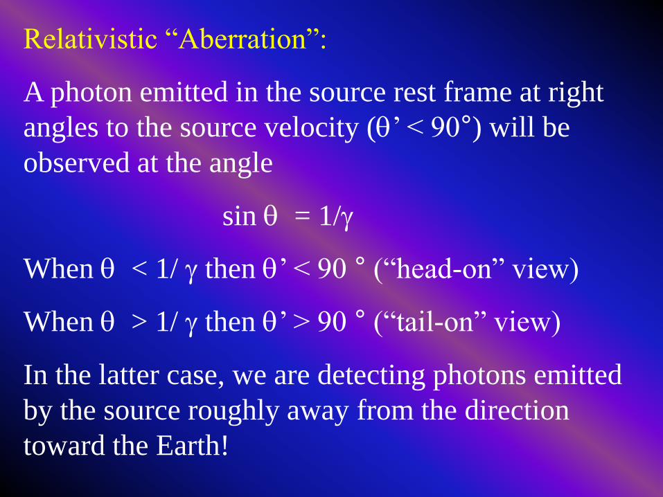
Relativistic “Aberration”:

A photon emitted in the source rest frame at right

angles to the source velocity (’ < 90°) will be

observed at the angle

sin = 1/

When < 1/ then ’ < 90 ° (“head-on” view)

When > 1/ then ’ > 90 ° (“tail-on” view)

In the latter case, we are detecting photons emitted

by the source roughly away from the direction

toward the Earth!

Series of images of an AGN

usually show apparent

superluminal motion due to

highly relativistic motion

close to line of sight.

Apparent observed speed is:

Where is v/c and is

angle of the jet to the line

of sight.

Linear polarization properties/

B-Fields of AGNs

Contour map taken from the Mojave website, sticks added to

illustrate various observed polarization patterns.

Polarization patterns observed for AGN jets on VLBI scales

B jet Bjet

Bjet

B jet

Some real examples

Mechanisms for generating B fields to jets

1) Transverse shocks — compress initially tangled B

field, field becomes ordered in plane of compression

Laing (1980)

Advantage: shocks can also help explain variability

Disadvantage: not natural way

to explain extended regions of

orthogonal B field

Cats imitating a tangled magnetic field.

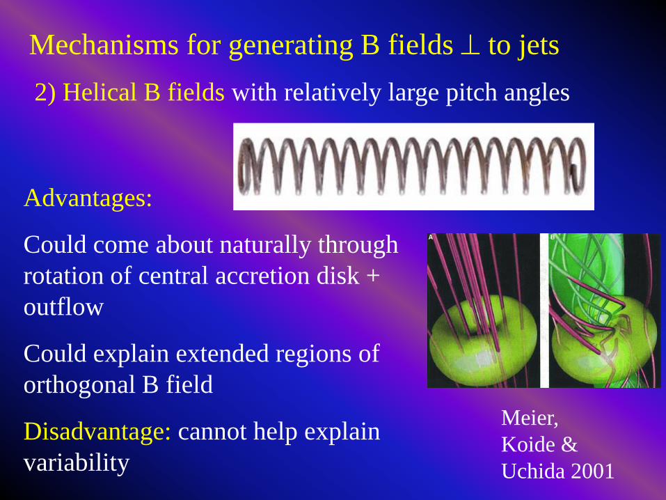
2) Helical B fields with relatively large pitch angles

Advantages:

Could come about naturally through

rotation of central accretion disk +

outflow

Could explain extended regions of

orthogonal B field

Disadvantage: cannot help explain

variability

Mechanisms for generating B fields to jets

Meier,

Koide &

Uchida 2001

Mechanisms for generating B fields || to jets

1) Shear interactions with ambient medium

Advantage: can explain extended regions of

longitudinal B field, if shear present all along jet

Disadvantage: local, no direct measurements of

velocity gradient toward edge of jet available

2) Helical B fields with relatively small pitch angles

Advantages:

Could come about naturally through

rotation of central accretion disk +

outflow

Could explain extended regions of

longitudinal B field

Mechanisms for generating B fields || to jets

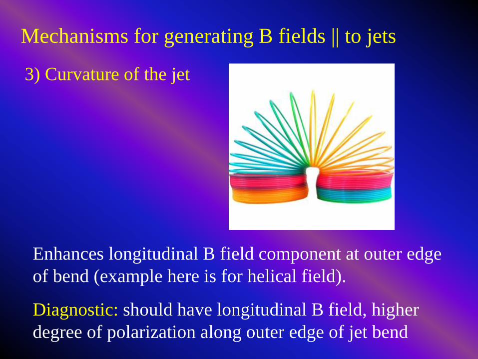
3) Curvature of the jet

Enhances longitudinal B field component at outer edge

of bend (example here is for helical field).

Diagnostic: should have longitudinal B field, higher

degree of polarization along outer edge of jet bend

Mechanisms for generating B fields || to jets

X

√

Tendencies for B-field structures in AGN jets

• Most complete studies carried out using MOJAVE

sample (Monitoring Of Jets in AGN with VLBA

Experiments) [e.g. Lister & Homan 2005]

• Core B fields often either or jet direction, but

can also have arbitrary orientations

• Jet B fields are predominantly or jet direction

Vector nature of field – if jet has cylindrical

symmetry, either or component will dominate

(e.g. Lyutikov et al 2005)

B-field structures in different AGNs

Quasars:

Strong optical emission lines

High radio luminosities

Relatively high apparent

component speeds

Longitudinal jet B fields

BL Lac objects:

Weak optical emission lines

Lower radio luminosities

Relatively low apparent

component speeds

Orthogonal jet B fields

Possible scenarios to explain dichotomy

1) Shocks & shear

Quasars have faster, more stable jets than BL Lacs

harder for transverse shocks to form in quasar

jets, shear with surrounding medium gives

longitudinal B field (Gabuzda et al. 1994; Duncan

& Hughes 1994)

2) Helical jet B fields

Both quasars and BL Lacs have helical B fields,

faster jet speeds in quasars lead to lower pitch

angles observed fields in BL Lacs mostly

orthogonal, in quasars mostly longitudinal

(Gabuzda et al. 2000; Asada et al. 2002)

How to tie in observed speeds and B-field

structures with strength of optical line emission?

Baum, Zirbel & O’Dea (1995): Optical emission lines of

FRI radio galaxies are less luminous than those of FRII

RGs, due to weaker ionizing continuum in FRI galaxies.

Possible scenario:

FRI/BL Lac = weak ionizing continuum + low-power jets,

low jet speeds, jets with transverse shocks and/or high-

pitch-angle helical fields

FRII/Quasar = strong ionizing continuum + high-power

jets, high jet speeds, jets without transverse shocks and/or

low-pitch-angle helical B fields

Other types of B field structures “Spine+Sheath”

Competing mechanisms:

Shocks + shear (Attridge et al.

1999)

Helical B fields (Pushkarev et

al. 2005; see right)

B E

E

Cats illustrating a partial spine–sheath B-field

structure.

B

Jet

direction

B

Core region B-Fields of AGNs

Estimation of B field strengths

Difficult to use “obvious” direct approaches because

observed radio structures are often unresolved or

marginally resolved – don’t know size of emission regions.

For example, basic synchrotron radiation theory leads to

the relation (Longair 1981):

Although peak can be determined well from multi-

wavelength VLBI data, measured I is usually only a limit

due to unknown true size of emission region.

Schematic

from Kovalev

et al. (2007)

VLBI “core” = optically thick base of jet, moves further

down jet at increasingly lower frequencies (Blandford &

Königl 1979; Königl 1981)

VLBI images align on bright, compact cores rather than

optically thin jet features, absolute position info lost,

direct superposition yields incorrect alignment.

This is actual correct physical alignment!

Alignment techniques

o Based on comparing positions of optically thin features

Model fitting

Image cross-correlation analyses

o In practice – different approaches work best for different

source structures, but both can yield reliable alignments

Example of misaligned

(top) and correctly

aligned (bot)spectral-

index maps

(8.9–15.4 GHz)

Partially optically

thick observed “core”

Optically thin jet Theoretical picture

More recent studies:

O’Sullivan & Gabuzda (2010) — only a few sources, but 8

frequencies (detailed, redundant information)

Kovalev et al. (2009) — 29 sources, 2 frequencies

Sokolovskii et al. (2011) — 20 sources, 9 frequencies

Pushkarev et al. (2012) — more than a hundred well

studied (MOJAVE) sources, four frequencies

Lobanov (1998):

o Approach to estimating pc-scale B field strengths

based on measurement of frequency-dependent position

of VLBI core (Konigl 1981)

o Few sources, few frequencies, but a start

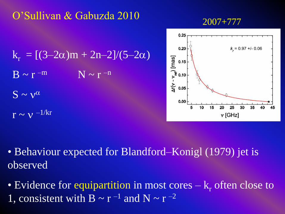
O’Sullivan & Gabuzda 2010

kr = [(3–2)m + 2n–2]/(5–2)

B ~ r –m N ~ r –n

S ~

r ~ –1/kr

• Behaviour expected for Blandford–Konigl (1979) jet is

observed

• Evidence for equipartition in most cores – kr often close to

1, consistent with B ~ r –1 and N ~ r –2

2007+777

• Inferred core-region B fields are tenths of Gauss

• Data consistent with B ~ r –1

• Extrapolation of B field to smaller scales gives values

consistent with magnetic launching of jets (points shown

are for rg and 10rg; Komissarov et al. 2007)

O’Sullivan & Gabuzda 2010

Pushkarev et al. (2012)

o Ability to compare shifts for

different types of AGNs.

o Shift distribution peaked in jet

direction, as expected

Pushkarev et al. (2012)

o B fields in quasars

somewhat higher than

in BL Lac objects

Quasar B fields at

1 pc ~ 0.9 G

BL Lac B fields at

1 pc ~ 0.4 G

Member of the UCC radio astronomy group

analysing the dynamics of a cloth model of a

core –jet source in a magnetic field.

Faraday Rotation

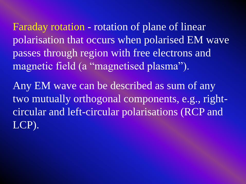
Faraday rotation - rotation of plane of linear

polarisation that occurs when polarised EM wave

passes through region with free electrons and

magnetic field (a “magnetised plasma”).

Any EM wave can be described as sum of any

two mutually orthogonal components, e.g., right-

circular and left-circular polarisations (RCP and

LCP).

EM wave propagates towards observer through region

with B field aligned with direction of propagation; free

electrons move in direction of E, giving rise to a

Lorentz force.

RCP and LCP

components obtain

different velocities

due to different

direction of Lorentz

force on free

electrons relative to

direction of rotation

of E vector.

Equations of motion of electron for RCP and LCP

components of EM wave:

Different indices of refraction for RCP and LCP components

of the EM wave in plasma with e- density n:

Different speeds of propagation of RCP and LCP

componts lead to a rotation in plane of linear

polarisation:

Amount of rotation:

• Linear dependence of rotation of polarisation angle on 2.

• Amount of FR depends on ne and line-of-sight B field

• Line-of-sight component of the ambient B field determines

sign of Faraday rotation.

Integrated Faraday

Rotaton of two

AGNs observed

with the VLA

(Wrobel 1993).

Zavala & Taylor (2003, 2004)

o 40 objects

o Core RM > Jet RM (higher ne and B?)

o Sometimes sign changes (changes in LOS B field)

o Quasar core RMs > BL Lac core RMs

If jet has a helical B field, should observe a Faraday-rotation

gradient across the jet – due to systematically changing line-

of-sight component of B field across the jet (Blandford 1993).

RM ~ ne B•dl

B

RM < 0

RM > 0

•

Jet axis

Simulation by

Broderick &

McKinney 2010

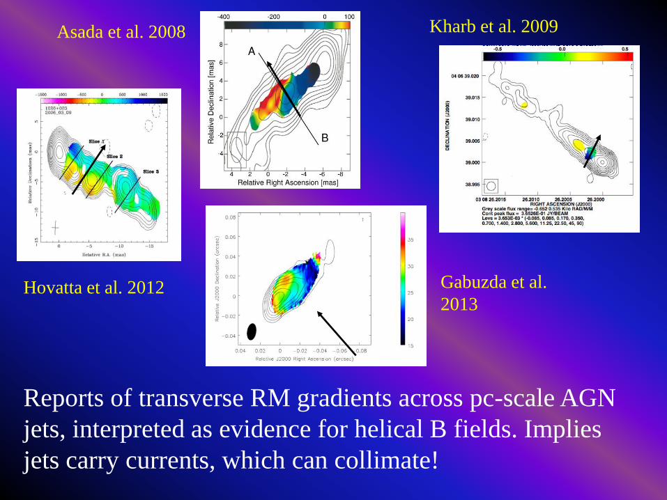
Reports of transverse RM gradients across pc-scale AGN

jets, interpreted as evidence for helical B fields. Implies

jets carry currents, which can collimate!

Hovatta et al. 2012 Gabuzda et al.

2013

Kharb et al. 2009 Asada et al. 2008

Is the field toroidal or helical?

Key difference: A toroidal field should not give rise to

asymmetrical transverse intensity and polarization profiles,

but a helical field can.

Observation of asymmetrical transverse profiles provides

evidence for helical, not just toroidal, fields.

Toroidal

Helical

Asymmetric transverse

pol structure

Transverse RM

gradient

===> Helical (not just toroidal) field present on pc scales

+

Example – 1633+382

(Coughlan & Gabuzda 2013)

Hope you’re not yet catatonic!

Circular Polarisation and

Faraday Conversion

Intrinsic circular polarisation (CP) of synchrotron

radiation is low, << 1% for typical core B fields of 0.1–

1 G — while observed CP in AGN cores is a few tenths

of a percent (e.g. Homan & Lister 2006).

More efficient mechanism: Faraday conversion of linear

polarisation (LP) to CP when EM wave passes through

magnetised medium (Jones & O’Dell 1977).

— Describe wave’s E field using components parallel to

(E||) and orthogonal to (E) B field in the medium Bmed

— Free charges in medium can be accelerated by E||, but

not by E (charges can’t move Bmed)

— E || is absorbed + re-emitted (delayed) while E is not

circular polarisation

Delaying one E component relative to the other is

equivalent to introducing a circularly polarised

component (figure from Gabuzda et al. 2008):

No Faraday conversion will occur when

— LP (E) is orthogonal to Bmed (electrons in medium

cannot move orthogonal to Bmed, E is not absorbed)

— LP (E) is parallel to Bmed (all of E is absorbed and re-

emitted)

— most efficient when LP (E) neither || nor to Bmed.

This makes Faraday conversion efficient in jets with helical

B fields (Homan & Wardle 2003, Gabuzda et al. 2008):

• LP emitted at “back” of jet (Esynch) is converted to CP as it

passes through the foreground helical B field at “front” of

jet (Bhel,fg)

• sign of CP determined by pitch angle & helicity of field

• provides hope for relating observed RM gradients and CP

to properties of associated helical jet B fields

Esynch,

LP

Bhel,fg

A cat who has found something far more interesting

than Active Galactic Nuclei!

tmeas = dlos/c = (ct - v cos t)/c

tmeas = (1 - cos ) t = v/c

vapp = dsky/ tmeas =v sin t/ (1 - cos ) t

Derivation of SLM

Measured time between

arrival of two photons

emitted by source moving

roughly toward observer at

times separated by time t

(observer’s frame) will be

Summary – B-field structure

Jet B fields of AGNs are usually either parallel to or

orthogonal to jet direction, expected if jets have

roughly cylindrical symmetry

Core polarizatons show larger range of orientations

(reflects higher Faraday rotation present in core region)

Various mechanisms can give rise to parallel or

orthogonal B fields – shocks, shear, curvature, helical

B fields. Sometimes not easy to distinguish!

Helical can be distinguished from toroidal B fields by

their asymmetric transverse polarisation structure

Summary - Core B fields

• Core B-field studies now carried out for large numbers

of frequencies and large source samples for the first time

• Most results consistent with equipartition in core region

• 15-GHz core B fields range from ~ 0.02 G – 0.8 G

• Data usually consistent with B ~ r –1

• Parsec-scale B fields extrapolated to much smaller

scales consistent with those predicted for magnetically

launched jets

• Core B fields somewhat lower in BL Lac objects

than in quasars

Summary – Faraday Rotation

• Core RMs > Jet RMs (higher e– density and B fields),

core RMs lower in BL Lacs than in quasars

• Transverse RM gradients provide direct evidence for

helical/toroidal jet B fields

— Jets are fundamentally EM structures, and carry

current, which has implications for collimation

• Evidence for return field in region surrounding the jet

• Preference for CW RM gradients across AGN jets

(inward axial currents) on pc scales, requires coupling

between rotation and axial jet B fields – action of a

“Cosmic Battery”? (Contopoulos et al. 2009;

Christodoulou et al. 2015).

Summary – Circular Polarisation

• When detected, circular polarisation usually found in

VLBI core, at levels of a few tenths of a percent

• Almost certainly due to Faraday conversion, which is

much more efficient at generating CP than intrinsic

synchrotron radiation, other conditions being equal

• May be efficient in presence of helical jet B fields,

providing hope of carrying out joint analyses of pol

structure, Faraday rotation structure and CP degree and

sign in core