The Quality of Labor Relations and Unemployment

Olivier Blanchard and Thomas Philippon∗

November 26, 2006

Abstract

There is a clear negative relation across OECD countries between measures of the qual-ity of labor relations and unemployment. We argue that conflictual labor relations causehigh unemployment, and we propose a model to think about this issue. Empirically,we use historical evidence from the 19th century to construct an instrument for currentlabor relations and establish causality. Theoretically, we consider an economy whereasymmetric information can result in bargaining failures, inefficiencies and high unem-ployment in equilibrium. These inefficiencies can however be alleviated by higher trust,sustained through repeated interactions between firms and workers. We think of coun-tries with different labor relations as playing different equilibria of the same repeatedgame, and we use our model to interpret cross-country and time series facts about laborrelations, strikes, and unemployment in OECD countries since the early 1970s.

∗MIT and NBER, and NYU and NBER respectively. An earlier version of this paper circulated as MITWP 04-25. Much of the empirical evidence and the model developed in this version are new. We thankPierre Cahuc, our discussant at the IZA-PSE workshop on cultural economics. We are indebted to YoungjinHwang for excellent research assistance.

1

There is a clear negative relation across OECD countries between measures of the qual-

ity of labor relations and unemployment. In this paper, we argue that this relation is

causal, and offer a framework to think about the relation between the two. We consider

an economy where asymmetric information can result in bargaining failures, inefficiencies

and high unemployment. These inefficiencies can however be alleviated by higher trust,

sustained through repeated interactions between firms and workers. We show how the equi-

librium degree of trust, which we think of as capturing the quality of labor relations in our

model, depends on both economic and non economic factors (history). We then use our

model to interpret cross-country and time series facts about labor relations, strikes, and

unemployment in OECD countries since the early 1970s.

In section 1, we study the empirical relation between labor relations, strikes, and un-

employment across OECD countries since the early 1970s. We focus first on the relation

between labor relations and unemployment. Looking across OECD countries, we show that

countries with better labor relations have experienced a lower increase in unemployment.

Using different instruments, we argue that this relation is causal, going from the quality

of labor relations to unemployment. We then turn to the relation between labor relations,

strikes, and unemployment. We show that the quality of labor relations is highly correlated

with strikes in the 1960s — i.e. with strike activity before the increase in unemployment.

We show that, until the early 1980s, countries where unemployment rates increased more

also experienced a larger increase in strike activity. Since the early 1980s, however, strike

activity has decreased, often dramatically, while unemployment has remained high in many

countries.

In section 2, we present our benchmark model. The model is an extension of the stan-

dard search model to a setup with asymmetric information and bargaining failures. We

model repeated interactions between the firm and its workers, so that inefficiencies might

be alleviated by the reputation of the firm. In section 3 we characterize the properties of the

equilibrium, and in particular the equilibrium degree of trust — defined as the proportion of

firms with good reputation — the variable which captures the quality of labor relations in

our model. The economic environment pins down the maximum sustainable degree of trust,

but the actual degree of trust can be anywhere between zero and this maximum. Thus, for

a given economic environment, some countries might have good labor relations, and some

2

might have bad labor relations. The countries with bad labor relations will have higher

unemployment, and will be more strongly affected by shocks that increase the amount of

firm-level asymmetric information. If the economic environment deteriorates, the maximum

sustainable degree of trust may itself decrease. This may lead to a decrease in the actual

degree of trust, to a deterioration of labor relations, and thus to a further effect of the

shocks on unemployment.

In section 4, we show how this model can potentially explain the cross-country relation

between the quality of labor relations and the rise of unemployment. The model also

naturally explains how the increase in unemployment was accompanied with an increase

in strikes. What it does not explain however is why strike activity has decreased so much

since the 1980s, while unemployment remained high in many countries. We argue that to

explain this fact, one needs to endogenize the technological choice of firms.

This leads us, in section 5, to extend our model to allow firms to adapt their technology in

response to deteriorating labor relations. We show how this extended model can potentially

account both for the cross country and time series facts presented in section 1.

1 Empirical Evidence

Figure 1 shows the strong negative cross-country correlation across 21 OECD countries

between the unemployment rate in 2000 and the quality of labor relations, as reported in

the 1999 Global Competitiveness Report. The measure of the quality of labor relations

is constructed from the answers to the following question:“Labor/employer relations are

generally cooperative”. The 1999 survey was sent to about 4,000 executives in 59 countries.

Responses could vary from 1 (strong disagreement) to 7 (strong agreement). Actual mean

responses vary from 3.3 for France to 6.4 for Switzerland.1

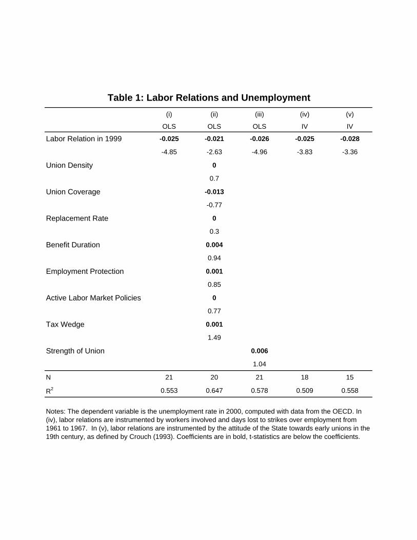
The first column of Table 1 presents the results of the associated OLS regression: The

quality of labor relations is highly statistically and economically significant. The R2 is 0.55,

and an increase in the measure from 3.3 to 6.4 is associated with a decrease in the unem-

ployment rate of 7.7 percentage points. The second column shows that the measure remains

1The same question was asked in a number of GCR surveys, starting in 1993; the measures are highlycorrelated, the rankings very stable, and the results very similar using earlier or later measures. For moredetails on this and other survey-based measures, see Mueller and Philippon (2006).

3

significant when one controls for other labor market institutions, taken from Blanchard and

Wolfers (2000). Once the quality of labor institutions is allowed for, formal institutions do

not appear to be very significant. In particular, union density and union coverage are not

significant. The third column shows that the quality of labor relations is not a proxy for the

bargaining power of unions. It does so by adding as an additional variable in the regression a

measure of union strength taken from the same survey. The measure is constructed from the

answer to the question: "The collective bargaining power of workers is high." The answer to

the question can vary from 1 (strong disagreement) to 7 (strong agreement). Actual mean

responses vary from 3.4 for Switzerland to 5.8 for Finland. The quality of labor relations

remains highly significant, while union strength is not.

The fourth and fifth columns turn to causality. The first potential source of endogeneity

is that different countries may have been hit by different shocks between 1970 and 2000:

Countries with worse shocks might have experienced both higher unemployment, more

downsizing of firms, and thus worse labor relations. To deal with this type of endogeneity,

we use measures of strike activity in the 1960s as instruments — i.e. measures of strike

activity before the shocks that led to the eventual increase in European unemployment.2

Two measures of strike activity are available for most countries and most years for the

1960s, namely the number of workers involved in labor conflicts (WI) and the number of

work-days not worked (DL). We use both, each per worker employed.3 The two measures

are highly but not perfectly correlated.4. Two empirical issues arise: The first is how to treat

Portugal and Spain, which were dictatorships and where strikes were illegal in the 1960s.

The wage explosion that took place in the two countries upon the end of the dictatorship

suggests that the true measure of trust was in fact quite low in the 1960s. But we have no

way to take this into account and so drop both countries from the sample in the relevant

regressions. The other is how to treat the years 1968 and 1969, where, in a number of

countries, most notably France and Italy, there was high labor unrest and unusually high

2A better instrument would be a measure of the quality of labor relations pre-1970. We could not findsuch a measure.

3The data come from the CEP-LSE data set. A third measure available in that data set, namely thenumber of conflicts, is missing too many observations for us to use it.

4 “Days lost” is not defined consistently across countries. For instance, it sometimes includes only conflictswith more than 100 days lost (Germany), or it includes strikes only (as opposed to strikes plus lock-outs)for France. As a consequence, the ratio of DL/WI in the 1960s is more than 10 times lower in France thatin the US. See Hibbs (1987)

4

levels of strikes. On the argument that these episodes reflected other factors than the one

we want to capture, we construct our measure of strikes by using average strike activity

over the period 1960 to 1967 rather than over the whole decade (Given that France and

Italy are high unemployment countries, our results below would actually be stronger, were

we to use the whole decade to construct the mean.)

To give a sense of the relation between strike activity in the 1960s and the quality of

labor relations today, we plot in figure 2 our measure of the quality of labor relations in

1999 against a synthetic measure of strike activity in the 1960s, constructed as Conf60i =

max³

DLi/Ni

std(DLi/Ni), WIi/Ni

std(WIi/Ni)

´, where DLi are days lost, WIi are workers involved, and

Ni is the number of employees in country i. The motivation for this specification is that

recorded strikes happened for sure, but not all strikes are recorded, so that both measures

are lower bounds on strike activity. The figure shows that higher strike activity in the

1960s is clearly associated with lower quality of labor relations today. The fourth column

of Table 1 shows the results of IV estimation, using both DLi/Ni and WIi/Ni (and not

the synthetic measure) as instruments for current labor relations. It shows that our earlier

OLS results are not driven by reverse causality from bad shocks to bad labor relations. The

point estimate on the quality of labor relations does not change much relative to the OLS

regression, perhaps because countries were hit by roughly similar shocks.

A second type of endogeneity is that both strikes in the 1960s and unemployment rates

are driven by the same unobserved country characteristics. To deal with this issue, we

borrow the theory of Crouch (1993) as explained in Mueller and Philippon (2006). Crouch

(1993) argues that labor relations were strongly influenced by the attitudes of the state

towards early unions in the 19th century. He distinguishes three categories of countries. In

four countries, the state was hostile towards the unions: France, Italy, Spain and Portugal.

In five countries, the state was neutral: Denmark, Norway, Sweden, Finland, the UK and

Ireland. In four countries, the state was supportive: Germany, Switzerland, the Netherlands

and Austria. Finally, Belgium borrowed from both the French and Dutch traditions: for

much of the 19th century, it was heavily influenced by France, but the Guilds of the great

Flemish cities played an important role in building the state, like in Germany. On balance,

we therefore put Belgium together with the neutral states.5

5Crouch actually goes further and provides a theory for the attitudes of the states based on the political

5

The fifth column of Table 1 reports the results of IV estimation using Crouch’s cat-

egories as instruments for the quality of labor relations. The IV regression confirms that

hostile labor relations cause high unemployment, and once again, the coefficient appears to

be quite stable.

We now turn to the evolution of labor relations, strikes, and unemployment over time.

We have no direct measure of labor relations before 1993, but the evidence since 1993 (the

first time the GCR survey asked the question) suggests that the quality of labor relations

is rather stable over time. Figures 3 and 4 then present the evolution of unemployment

and strike activity (using days lost per worker, the only series available for each country

for the whole sample) for the three categories defined by Crouch — hostile, neutral, and

cooperative. The figures show that, from the late 1960s to the late 1970s, both strikes and

unemployment increased, more so in countries with hostile labor relations. Since the early

1980s, however, unemployment has increased or at least stayed constant, but strikes have

decreased, especially in countries with bad labor relations, to the point that strike rates are

now roughly similar in all the countries in our sample.

Our goal in the rest of the paper is to provide a model and offer interpretations for these

facts.

struggles with the catholic church. He argues that, to affirm their authority over the Catholic church, liberalstates confronted all forms of organized interests, including guild structures and labor organizations. Bydoing so, these states created hostile labor unions. By contrast,

"Lutheran churches have historically been obedient national institutions, [. . . ] asserting nosuperior political loyalty as did the Vatican-based Catholic Church [...] This lack of ‘jealousy’reduced the extent to which these states confronted guilds and subsequently provoked theformation of highly oppositional labor movements." Crouch (1993)

Note that Crouch (1993)’s theory is not about religion as such, but about politics: according to him, whatmattered were the state-church conflicts created by the political ambitions of the Catholic church, not thefact that citizens of these countries happened to be catholic. Of course, one would expect the conflicts tobe stronger in more catholic countries, but there are two illuminating exceptions. The first is Ireland, whichwas under British rule at the time of the creation of labor unions. Therefore, early Irish labor institutionsresemble the British ones, and differ greatly from those of other catholic countries. The second exception isAustria, which took Germany as a role model, and in which state-church conflict were remote because thestate was very weak. As a result, early Austrian institutions resemble German ones. It seems plausible thatthe state-church conflicts of the 19th century do not affect unemployment directly today, so we can use theCrouch classification as a valid instrument.

6

2 Benchmark Model

A natural formalization approach, given our goals, is to introduce asymmetric information

in an otherwise standard matching/search model of the labor market.

We start by describing the stage bargaining game between workers and firms in section

2.1. We consider the non-cooperative outcome of the stage game in section 2.2, and the

cooperative outcome in section 2.3. We describe the macroeconomic closure in section 2.4.

Section 3 characterizes the equilibrium level of unemployment as a function of the proportion

of firms with good reputation — the degree of trust for short — and the equilibrium range

for the degree of trust, and its dependence on economic and non economic factors.

2.1 Bargaining Game

Once a firm and a worker have matched, the initial productivity of the match is revealed

to the firm, but not to the worker. Productivity, y, can take one of two values, yh with

probability p, or yl with probability 1 − p. We assume that yh > yl > 0 and we define

average productivity as y ≡ p yh + (1 − p) yl. Productivity remains constant until, with

probability λ per unit of time, a new productivity is drawn from the same distribution, and,

with probability δ per unit of time, the match becomes unproductive and ends.

We denote the reputation of the firm by the variable ρ. The reputation of the firm

can be good, ρ ≡ g, or bad, ρ ≡ b. Associated with the two levels of productivity are the

ongoing match-surpluses S(yh, ρ) and S(yl, ρ). The relation of the surplus to productivity

depends on the rest of the model and will be derived later. We will later assume that the

surplus is positive even if productivity is low, so that matches should never be dissolved.

The average surplus is denoted S (ρ) ≡ Ey [S(y, ρ)].

Let U denote the value for the worker of being unemployed and V the value for the firm

of having a vacancy. Let J(y, ρ) and W (y, ρ) be respectively the values for the firm and for

the worker of being in an ongoing match with productivity y and reputation ρ. Then, by

definition,

J(y, ρ)− V +W (y, ρ)− U = S(y, ρ). (1)

Bargaining determines the values of J(y, ρ) and W (y, ρ) given S(y, ρ), V and U . We for-

malize bargaining as follows:

7

• The firm makes an offer W .

• The worker either rejects the offer, with probability s, or accepts the offer, with

probability 1− s. The probability of rejection is endogenous and will be determined

in equilibrium. In particular, it will be a function of the reputation of the firm.

• If the worker accepts the offer, the match takes place.

• If the worker rejects the offer, a fraction γ of the match-surplus is destroyed. The

worker then makes a take-it or leave-it counter-offer W c. If the firm rejects the offer,

the match ends.

An alternative formalization would be that, with probability γ, the match ends. This

alternative formalization makes no difference to the bargaining game, but it creates

inefficient separations and additional flows into unemployment, and so affects equilib-

rium unemployment. We shall return to this formalization choice later on, when we

simulate the model.

We focus on the separating equilibrium, where the firm tells the truth about productivity.

Under that condition, we can solve for the equilibrium backwards. The counteroffer by the

worker will clearly be such as to extract all the surplus from the match. Thus

W c(y, ρ) = U + (1− γ)S(y, ρ), (2)

and, from (1),

Jc(y, ρ) = V.

The lowest initial offer by the firm that the worker will accept is therefore

W (y, ρ) =W c(y, ρ) = U + (1− γ)S(y, ρ), (3)

which implies

J(y, ρ) = V + γS(y, ρ). (4)

The firm gets a share γ of the surplus, the worker a share 1−γ. The parameter γ therefore

captures the bargaining power of the firm.

8

The key issue is how firms are induced to tell the truth. We consider two cases: non-

cooperative Nash equilibrium played by firms with a bad reputation, and cooperative equi-

librium sustained by good reputation. Let μ and 1− μ be the fractions of firms with good

reputation and bad reputation, respectively. For the moment we take μ as given.

2.2 Non Cooperative Equilibrium

A fraction 1 − μ of the matches have a bad reputation, ρ = b. These firms play the non-

cooperative equilibrium. The worker does not observe the productivity of the match. The

firm must therefore have the correct incentives the tell the truth. If productivity is high,

the value for the firm of telling the worker that productivity is high must be at least equal

to the value of telling the worker that productivity is low. Thus, the truth telling constraint

is

S³yh, b

´−W (yh, b) ≥ (1− s)(S(yh, b)−W (yl, b)) + s

³(1− γ)S(yh, b)−W c(yl, b)

´.

The LHS gives the value to the firm of telling the worker that productivity is high. The

RHS gives the expected value of telling the worker instead that productivity is low. The

first term represents the value to the firm if the worker accepts the offer W (yl), something

that happens with probability 1−s. The second term represents the value to the firm if theworker rejects its initial offer and makes the counteroffer W c(yl), something that happens

with probability s. Using the equations (2) and (3) above, the constraint can be rewritten

to give the equilibrium probability of a rejection. Assuming the earlier condition holds as

an equality (there is no reason for workers to choose a higher rejection probability than the

minimum required to induce truth telling), we obtain

s (b) =1− γ

γ

S(yh, b)− S(yl, b)

S(yh, b). (5)

The probability of a rejection when the firm announces that productivity is low is an

increasing function of S(yh, b) − S(yl, b). Given that the firm gets a share of the surplus,

the higher the difference between the surplus in the high and low productivity states, the

larger the value to the firm of announcing low productivity when productivity is in fact

high, and so the higher the probability of a rejection required to deter the firm from lying.

The positive probability of a rejection creates an inefficiency. The average deadweight loss

9

due to asymmetric information is given by

D (b) = (1− p) s (b) γ S(yl, b). (6)

It is useful to compute the average value of a match to a worker and to a firm, pre-bargaining.

Denote them by Wλ and Jλ. They are given by

Wλ (ρ) = U + (1− γ)S (ρ) , (7)

and

Jλ (ρ) = V + γS (ρ)− D (ρ) . (8)

Note that the partial equilibrium incidence of the deadweight loss falls fully on the firm,

not on the worker.

2.3 Cooperative Equilibrium

A fraction μ of firms have a good reputation, ρ = g. The cooperative equilibrium is

sustained by a trigger strategy. If the firm ever lies, the reputation of the firm switches to

ρ = b and bargaining becomes non-cooperative, as described in the previous section. Note

that productivity is observable after bargaining, so that the worker can observe ex-post

whether the firm has told the truth or not. Reputation is match specific, and ends with the

end of the match (a δ shock). The critical constraint in this dynamic game is the dynamic

truth-telling constraint

S(yh, g)−W (yh, g) +λ

r + δ + λJλ(g) > S(yh, g)−W (yl, g) +

λ

r + δ + λJλ(b).

The issue of whether the firm will tell the truth arises only if productivity is high and the

firm has a good reputation. The benefits from telling the truth are given by the LHS, the

benefits from not telling the truth by the RHS. Not telling the truth increases the part of

the surplus going to the firm today, but at the cost of a bad reputation in future bargaining.

Naturally, we have

D (g) = 0.

since workers never reject the offers from firms with a good reputation.

Using equations (7) and (8), we can rewrite the truth-telling constraint as

(1− γ)(S(yh, g)− S(yl, g)) ≤ λ

r + δ + λ

£D(b) + γ

¡S (g)− S (b)

¢¤. (9)

10

The LHS is the immediate payoff from giving a smaller fraction of the match surplus to

the worker, and the RHS is the NPV of the future losses from having a bad reputation.

The RHS has two component, the first is deadweight loss expected when bargaining takes

place in the future, and the second is the lost surplus. To draw further implications, we

need however to solve for the various surplus terms in equation (9), and so we turn to the

macroeconomic closure.

2.4 Macroeconomic Closure

The macroeconomic closure follows closely the standard matching/bargaining model:

• There is a mass of workers of size 1, with u workers unemployed, and 1− u workers

employed. The mass of vacancies is equal to v, and is endogenously determined.

• Matches are determined by a constant-returns matching function m(u, v). Defining

θ ≡ v/u, so θ measures the tightness of the labor market, the matching rate for

vacancies, q(θ) ≡ m/v = m(1/θ, 1) is a decreasing function of θ. The matching rate

for the unemployed is in turn equal to θq(θ) and is an increasing function of θ.

Given the equilibrium degree of tightness, unemployment dynamics follow

u = δ(1− u)− θq(θ)u.

Note that we have ruled out inefficient separations, and so the destruction rate is simply

δ. For u = 0 (as we are limiting ourselves to look at steady states), the equilibrium

unemployment rate is thus given by

u =δ

δ + θq(θ). (10)

3 Equilibrium

There are four steps needed to solve for the macroeconomic equilibrium:

• The first two are the same as in Pissarides (2000): we need to find the various valuefunctions, and then impose free entry. The free entry condition will give us a link

between market tightness θ and the deadweight losses from bargaining failures. Absent

11

these deadweight losses, this would be enough to solve for θ, like in Pissarides (2000).

Here, however, this is not enough since the deadweight losses from equation (6) are

endogenous.

• The third step uses the incentive constraint (5) to obtain the deadweight losses as afunction of θ and μ. After these three steps, we can solve for θ as a function of μ.

• The fourth and final step is to use the truth telling constraint (9) in order to computethe equilibrium range of values of μ.

We now detail these four steps.

3.1 Value Functions

The surplus associated with a match with productivity y and reputation ρ is given by:

rS(y, ρ) = y − r (U + V )− δS (y, ρ) + λ¡S (ρ)− D (ρ)− S (y, ρ)

¢.

The first two terms on the RHS give the flow value of the match, net of the opportunity

cost. The next term gives the capital loss associated with the end of the match, times

the probability that such a change takes place. The last term gives the expected capital

gain or loss associated with a new draw of productivity, times the probability that such a

change takes place. As we saw earlier, the expected value of the pre-bargaining surplus is

equal to the expected surplus net of the expected deadweight loss coming from the positive

probability of a bargaining failure. Define ∆ ≡ yh − yl, so that yh = y + (1− p)∆ and

yl = y − p∆. It follows from the equation above that S(y, ρ) is given by

S³yh, ρ

´= S (ρ) +

(1− p)∆

r + δ + λ, (11)

and

S³yl, ρ

´= S (ρ)− p∆

r + δ + λ, (12)

where S (ρ), the average surplus from a match with reputation ρ is given by

S (ρ) =y − r (U + V )− λD (ρ)

r + δ. (13)

12

These equations imply a simple relation between differences in productivity and differences

in the associated surplus

S³yh, ρ

´− S

³yl, ρ

´=

∆

r + δ + λ. (14)

We now need to derive the values of U and V . We assume that search is random. Therefore,

the worker has probability μ of matching with a firm with good reputation, and probability

1 − μ of matching with a firm with bad reputation. On average, the value of a match for

the worker is

Eρ£W e (ρ)

¤ ≡ μW e(g) + (1− μ)W e(b).

Let u the flow utility associated with being unemployed, and c be the flow cost of having a

vacancy. The value of being unemployed is

rU = u+ θq(θ)¡Eρ£W e (ρ)

¤− U¢, (15)

Using (7), we can rewrite (15) as

rU = u+ θq(θ) (1− γ)Eρ£S (ρ)

¤. (16)

Taking expectations of (13) with respect to reputation, we obtain

Eρ£S (ρ)

¤=

y − rU − (1− μ)λD(b)

r + δ,

and using (16) we get

Eρ£S (ρ)

¤=

y − u− (1− μ)λD(b)

r + δ + (1− γ) θq(θ). (17)

This is a familiar relation, giving the surplus as the properly discounted value of productivity

net of the flow utility of being unemployed. The difference is the presence of the deadweight

loss, coming from the fact that changes in productivity in the future may lead to a bargaining

failure.

3.2 Free Entry

The value of a vacancy is

rV = −c+ q(θ) (Eρ [Je (ρ)]− V ) , (18)

13

and the free entry condition implies that the value of a vacancy V must be equal to zero.

From equations (8), (18), and the free entry condition, we get

c

q(θ)= γEρ

£S (ρ)

¤− (1− μ)D(b). (19)

This is again a familiar relation, linking the degree of tightness to the average surplus from

a match. The difference with the standard case is the presence of the deadweight loss due

to asymmetric information and bargaining failures. The higher the surplus, or the lower

the deadweight loss, the tighter the labor market. To characterize the equilibrium in the

traditional search model, we usually combine (19) and (17). In our model, this leads to

c

q(θ)= γ

y − u− (1− μ)λD(b)

r + δ + (1− γ) θq(θ)− (1− μ)D(b). (20)

In the particular case where μ = 1 or D (b) = 0, we have the same model in Pissarides

(2000) and the above equation determines down the tightness of the labor market. In

general however, to solve our model, we must obtain a equation for D (b).

3.3 Deadweight Losses

We just obtained θ as a function of D(b) using the free entry condition. We now derive D(b)

as a function of θ from the non-cooperative IC constraint (5). Using (14), we can rewrite

(5) as

s (b) =1− γ

γ

∆

r + δ + λ

1

S(yh, b).

Replacing in (6) we get

D(b) = (1− p) (1− γ)∆

r + δ + λ

S(yl, b)

S(yh, b).

Using (11) and (12), we therefore obtain

D(b) = (1− p) (1− γ)∆

r + δ + λ

S (b)− p∆r+δ+λ

S (b) + (1−p)∆r+δ+λ

. (21)

where, from (13)

S (b) = Eρ£S (ρ)

¤− μλD (b)

r + δ. (22)

14

3.4 Characterization of Market Tightness

We have four equations (17), (19), (21) and (22) in four unknowns D(b), S(b), Eρ£S (ρ)

¤and θ. In the appendix, we derive the following proposition:

Proposition 1 For ∆ not too large:

1. The degree of labor market tightness, θ is an increasing function of the proportion of

firms with good reputation, μ and a decreasing function of ∆.

2. The deadweight loss, D(b) is a decreasing function of the proportion of firms with good

reputation, μ, and an increasing function of ∆.

Thus, the higher the degree of trust in the economy, the tighter the labor market — and

by implication, the lower the unemployment rate — and the lower the deadweight loss. The

higher the degree of uncertainty about productivity, the less tight the labor market — and

by implication, the higher the unemployment rate — and the higher the deadweight loss.6

3.5 Sustainable Equilibria

We have derived the equilibrium conditional on a given value of μ, the fraction of firms

with good reputation. The last step is to determine μ. Rewrite the dynamic truth telling

constraint (9) as

(1− γ)(S(yh, g)− S(yl, g)) ≤ λ

r + δ + λD(b)

∙1 +

γλ

r + δ

¸,

or

λ

∙1 +

γλ

r + δ

¸D(b) ≥ (1− γ)∆. (23)

An increase in r + δ shortens the horizon and makes trust harder to sustain. An increase

in λ, the probability of a new productivity draw and thus the probability of renegotiation,

makes reputation more valuable and easier to sustain. An increase in γ increases the surplus

going to the firm and makes it easier to sustain trust. Finally, the deadweight loss D(b)must

6This is subject to the caveat that ∆ not be too large. In our simulations, we have found the derivativesto satisfy the sign conditions of Proposition 1 for any ∆ satisfying the condition that the surplus from a lowproductivity match is positive. We have been unable, however, to prove it analytically.

15

be large enough since it represents the punishment in case the firm lies. The equilibrium is

described by the following proposition:

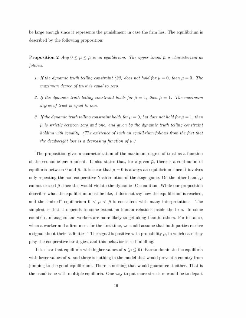
Proposition 2 Any 0 ≤ μ ≤ μ is an equilibrium. The upper bound μ is characterized as

follows:

1. If the dynamic truth telling constraint (23) does not hold for μ = 0, then μ = 0. The

maximum degree of trust is equal to zero.

2. If the dynamic truth telling constraint holds for μ = 1, then μ = 1. The maximum

degree of trust is equal to one.

3. If the dynamic truth telling constraint holds for μ = 0, but does not hold for μ = 1, then

μ is strictly between zero and one, and given by the dynamic truth telling constraint

holding with equality. (The existence of such an equilibrium follows from the fact that

the deadweight loss is a decreasing function of μ.)

The proposition gives a characterization of the maximum degree of trust as a function

of the economic environment. It also states that, for a given μ, there is a continuum of

equilibria between 0 and μ. It is clear that μ = 0 is always an equilibrium since it involves

only repeating the non-cooperative Nash solution of the stage game. On the other hand, μ

cannot exceed μ since this would violate the dynamic IC condition. While our proposition

describes what the equilibrium must be like, it does not say how the equilibrium is reached,

and the “mixed” equilibrium 0 < μ < μ is consistent with many interpretations. The

simplest is that it depends to some extent on human relations inside the firm. In some

countries, managers and workers are more likely to get along than in others. For instance,

when a worker and a firm meet for the first time, we could assume that both parties receive

a signal about their “affinities.” The signal is positive with probability μ, in which case they

play the cooperative strategies, and this behavior is self-fulfilling.

It is clear that equilibria with higher values of μ (μ ≤ μ) Pareto-dominate the equilibria

with lower values of μ, and there is nothing in the model that would prevent a country from

jumping to the good equilibrium. There is nothing that would guarantee it either. That is

the usual issue with multiple equilibria. One way to put more structure would be to depart

16

from the assumption of full rationality and argue that, in some countries, some workers do

not trust the firms, no matter what the firms do.7 In this case, μ becomes a function of the

fraction of hostile workers because the dynamic IC condition is more difficult to satisfy when

there are more hostile workers. We could then assume that countries always coordinate on

the Pareto dominating equilibrium, μ = μ, but this Pareto dominating equilibrium would

itself be a function of the historically given share of hostile workers. The results would be

essentially the same as those obtained here.8 Our model therefore offers an interpretation

of differences in the quality of labor relations as being based partly on economic factors,

and partly on non-economic factors. Economic factors, such as for example the degree of

uncertainty ∆, determine μ, the upper bound on the degree of cooperation. But given this

upper bound, the equilibrium degree of cooperation may be anywhere between 0 and μ.

This suggests the following approach. In looking at differences across countries, it seems

reasonable to start with the assumption that they are facing roughly the same economic

conditions, and that differences in the evolution of unemployment come from differences

in μ’s. In looking instead at movements in unemployment in a given country over time, it

seems reasonable to think of them as coming either from reactions to shocks for a given μ,

or from movements in μ, which, if binding, lead in turn to movements in μ. This is the

approach we follow in returning to the data in the next section.

4 Interpreting the Empirical Evidence

4.1 A Simple Case

To gain the basic intuition for the implications of the model, consider the case where ∆ is

small, and the first-order approximation to the deadweight loss around ∆ = 0 is given by:

D (b) ≈ (1− p)(1− γ)∆

r + δ + λ.

Consider two countries, one country with μ = 0 (say France for concreteness) and a country

with μ = 1 (say Denmark). From equation (20), equilibrium labor market tightness in

France is given by:c

q(θ)= γ

y − u− λD(b)

r + δ + (1− γ) θq(θ)− D(b),

7 It is tempting to replace “workers” by “unions”, as some European unions are notoriously distrustful offirms. But our model has only bilateral bargaining.

8This was the approach we followed in an earlier draft.

17

and, in Denmark, byc

q(θ)= γ

y − u

r + δ + (1− γ) θq(θ).

Now consider the effects of the same increase in ∆ in both countries. The increase in ∆ will

have no effect in Denmark, but will decrease tightness, and thus increase unemployment in

France. In other words, the lower the degree of trust, the worse the effects of an increase

in uncertainty. The underlying mechanism is straightforward: Higher uncertainty leads to

more strikes, thus to more bargaining failures, a lower surplus, and less entry by firms. This

is an example of interactions between shocks and institutions emphasized by, among others,

Blanchard and Wolfers (2000). The shocks is the same, but different institutions lead to

different outcomes.

Our model also implies another type of interactions, which may also be relevant. We

just assumed that μ remained unchanged in each country in the face of the increase in

uncertainty. But μ and by implication μ, may also decrease. This effect is not present

under our first-order approximation around ∆ = 0: In that case both the LHS and RHS of

the dynamic truth-telling condition are linear in ∆ so changes in ∆ do not affect whether

the condition holds, and thus do not change the equilibrium value of μ. But in the general

case, an increase in ∆ will indeed decrease μ. In words: The adverse shocks may lead to a

worsening of institutions, implying larger effects on unemployment.

4.2 A Calibration

To gain a sense of potential magnitudes, we now turn — with all the proper caveats — to a

calibration of the model. The parameter values we choose are given in the table below. The

choice of y − u is simply a normalization. We set c so that the benchmark unemployment

rate without asymmetric information is 6%. The values of r and δ are standard. The

parameter γ determines the capital share, so we choose it to be 1/3. We choose p < 1/2 so

that there is positive skewness in firm productivity, as in the data.

y − u δ r λ γ p

1 0.1 0.03 1 1/3 1/3

We then solve the model numerically. Figure 5 illustrates our results by plotting the

equilibrium unemployment rate as a function of the degree of trust μ and the amount of

18

firm level asymmetric information ∆. μ varies between 0 and 1, ∆ varies between 0.0 and

0.3 (the upper bound is thus equal to 0.3 of the net productivity of the match). For all the

values of ∆ within this range, μ is equal to 1, so all values of μ between 0 and 1 can be

equilibria. (The critical value of ∆ which would lead to a decrease in μ below one is equal

to 0.36). In this simulation, the maximum difference in unemployment between countries

with very good and very bad labor relations is 1.4%.

This is less than suggested by our regressions. Could the effect be larger? The answer

is yes. There is, within the logic of our model, one channel which can make it substantially

larger. Recall that we have assumed that bargaining failures lead to a lower surplus, but not

to separations. Thus, the consequences of bad labor relations is only through lower entry.

However, Bertola and Rogerson (1997) show that, despite stringent dismissal restrictions in

most European countries, rates of job creation and destruction are remarkably similar across

European and North American labor markets and suggest that this may be due in part to

inefficient separations. Our model provides an easy way to capture their hypothesis. We

only need to reinterpret the deadweight losses in case of bargaining failure as the probability

of an inefficient termination of the match. That is, with probability γ, a rejection leads to

the destruction of the match. This leaves the bargaining game unchanged, as well as all the

value functions. In fact, the only equation that needs to be modified is the unemployment

equation. Let us define the average inefficient destruction rate conditional on bargaining by

δ ≡ (1− μ) (1− p)γs (b) .

Unemployment dynamics are then given by

u = (δ + λδ) (1− u)− θq(θ)(1− δ)u.

This equation reflects the fact that some separations are due to bargaining failures in re-

sponse to changes in the productivity of existing matches, and some hiring do not lead to a

match, again due to a bargaining failure. For u = 0, we can then replace equation (10) by

u =δ + λδ

δ + λδ + θq(θ)(1− δ).

Figure 6 plots unemployment as a function of μ and ∆, but now under the assumption that

all bargaining failures lead to separations. The quantitative impact of inefficient separations

19

is very large — probably too large. The shape of the unemployment rate looks very similar to

the one in figure 5, starting at 6%, but the maximum value is 15.3% instead of 7.4%. Thus,

if all bargaining failures result in inefficient separations, the model can explain differences

unemployment of 8% or more. This happens because the inefficient separation rate λδ can

be as high as 11%, roughly doubling the total separation rate in the economy.

4.3 Pre-1980 and Post-1980 Outcomes

We can now go back to the evidence in Figures 3 and 4. One practical issue is how to

relate the bargaining failures in our model to strikes in the data. It is clear that not all

bargaining failures lead to strikes (see Gary-Bobo and Jaaidane (2006) for a discussion). It

seems plausible, however, that some bargaining failures lead to strikes. If we assume that

the probability that a bargaining failure translates into a strike stays roughly constant over

time, then we can use the strike rate as a qualitative proxy for bargaining failures.

If we do so, our model provides a natural explanation for the pre-1980 evolution of

strikes and unemployment. Countries differ in the quality of labor relations. Faced with

similar adverse shocks, they reacted differently. Both strikes and unemployment increased

more in countries with bad labor relations. In the absence of data on the evolution of labor

relations during that period, it is impossible to say whether this was also accompanied by a

decrease in the fundamental quality of labor relations within some countries. To the extent

that it was, the adverse effects of the shocks on unemployment were reinforced.

The model however does not do well in explaining what has happened since 1980, namely

the dramatic decline in strikes, together with a continued increase in unemployment. Within

the model, this is not easy to explain. We have explored whether other shocks than increases

in ∆ may explain both an increase in unemployment and a simultaneous decrease in strikes.

A decrease in y−u does not work, because it increases strikes and unemployment together.The intuition for the increase in unemployment is the usual one. The intuition for the

increase in strikes is that a lower surplus leads to an increase in rejection to keep the incentive

constraint satisfied. If the μ were binding, a decrease in y − u would also make it harder

to sustain trust. A increase in c goes in the right direction. It increases unemployment

by making it more costly to post a vacancy. It decreases strikes because it increases the

equilibrium match surplus. Starting from our benchmark case, for an economy with μ = 0.5

20

— an economy where half the firms have a good reputation — doubling the entry cost would

reduce the rejection rate by half. Thus, increases in c have the potential to account for

the post 1980 experience, but the changes would have to be very large.9 This leads us to

explore, in the next section, an alternative explanation, based on endogenous technological

choice.

5 Endogenous Technology

Faced with bargaining failures and strikes, firms are likely to change their technology or

their activity so as to reduce either the likelihood or the cost of bargaining failures. One

way to do so is for firms to reduce the role of labor in production, and thus reduce the stakes

involved in bargaining with labor. This type of choice has been explored by Caballero and

Hammour (1998), who explore the idea that an increase in bargaining power by workers in

Europe in the 1970s may have led firms to shift to more capital intensive techniques in the

1980s and the 1990s, resulting in higher unemployment, and a lower labor share. Another

direction is for firms to reduce the uncertainty associated with their activities, for example

by choosing products with more stable demand over new products, or more established

technologies over new technologies. This is the direction we explore here. Within the model

we have developed, we now allow firms, when they open a vacancy, to choose between two

technologies:

• The first technology is the one described above. The flow cost is c, the expected

surplus going to capital owners is

Jλ − V = γEρ£S (ρ)

¤− (1− μ)D(b),

and the value of a vacancy is given by

V =q(θ)Jλ − c

r + q(θ).

9An interpretation which is sometimes given for these joint fact is that high unemployment has madeit very costly for workers to go on strike and risk being unemployed. Our assumptions about bargainingdo not however deliver such an outcome, as the value of being employed and unemployed move largelytogether. This aspect, which is not specific to our model, may perhaps be seen as a shortcoming of this classof search/bargaining models.

21

• The second technology has ∆ = 0, but a higher entry cost co > c (this is nearly

equivalent to assuming a lower value for productivity, but slightly simpler analytically.

The surplus going to capital owners is

Jo − V = γSo,

where

So =y − u

r + δ + (1− γ) θq(θ),

and the value of a vacancy is given by

V o =q(θ)Jo − co

r + q(θ).

• Firms choose optimally which type of vacancy to open

V = max³V , V o

´.

and free entry implies that V = 0.

It follows from the equations above and from equation (17) that the safe technology

dominates the risky one if and only if

(1− μ)D(b)

µ1 +

γλ

r + δ

¶>

co − c

q(θ). (24)

Assume that initially μ < 1 and that all firms are using the uncertain technology. Now con-

sider an increase in ∆. We know from Proposition 1 that the deadweight loss D(b) increases

and labor market tightness decreases. Both make the inequality more likely to hold, and

so, for some critical value of ∆, firms shift to the safe technology, eliminating bargaining

failures. Thus, increases in uncertainty lead initially to an increase in unemployment and

strikes, until firms shift to the certain technology. At that point, further increases in ∆ no

longer have an effect on unemployment, and strikes remain equal to zero.

The extended model suggests a straightforward explanation for the facts in figures 3

and 4. Starting in the 1970s, firm-level uncertainty increased. In countries where the degree

of trust was high, this had little effect on either unemployment or strikes. In countries with

a low degree of trust, the result was an increase in both unemployment and strikes. It even-

tually became profitable for firms in those countries to shift to a more certain technology.

As a result, unemployment has remained high, but strikes have decreased.

22

6 Conclusion

We see our paper as making two main contributions: The first is to document the strong, and

apparently causal relation, between the quality of labor relations and unemployment. Given

the standard focus on formal institutions, we see this as an important empirical finding. The

second is to provide a natural framework in which to make the notion of “quality of labor

relations” more precise, and to think about its determinants and its economic implications.

Further research is needed to better understand the economic implications of trust be-

tween workers and firms. We have focused on the implications of the quality of labor

relations on bilateral bargaining. Bad labor relations may however have an impact through

collective bargaining, say the ability of an economy to adjust to changes in terms of trade

or in productivity growth. This remains to be satisfactorily formalized. We have left open

the question of whether bargaining failures lead to lower surpluses or/and inefficient sep-

arations. This is an important issue, both theoretically and empirically. Finally, we have

focused on an increase in firm level uncertainty as a major shock in our interpretation of the

facts. While it is widely believed that uncertainty faced by firms has increased as a result of

globalization and higher competition, and a similar idea has been explored by other authors

working on unemployment (Ljungqvist and Sargent (1998) for example), hard evidence has

been difficult to come by.

We have offered an interpretation of the decrease in strike activity since the early 1980s

based on endogenous technology. We see this as an appealing explanation, but we admit

that the evidence in support is mostly the very fact we want to explain, namely sustained

unemployment and the decrease in strikes. Harder evidence is needed here as well. The

choice of lower return/lower risk technologies, may well have important implications for

growth. Testing whether this channel is indeed important will probably require the use of

firm level data.

23

References

Bertola, G., and R. Rogerson (1997): “Institutions and Labor Reallocation,” European

Economic Review, 41(6), 1147—1171.

Blanchard, O., and J. Wolfers (2000): “Shocks and Institutions and the rise of Euro-

pean unemployment. The aggregate evidence,” Economic Journal, 110(1), 1—33.

Caballero, R. J., and M. L. Hammour (1998): “Jobless Growth: Appropriability, Fac-

tor Substitution, and Unemployment,” Carnegie-Rochester Conference Series on Public

Policy, 48(0), 51—94.

Crouch, C. (1993): Industrial Relations and European State Traditions. Clarendon Press,

Oxford.

Gary-Bobo, R., and T. Jaaidane (2006): “Strikes as the ’tip of the Iceberg’ in a Theory

of Firm-Union Cooperation’,” Working Paper, Universite Paris I.

Hibbs, D. (1987): The political economy of industrial democracies. Harvard University

Press.

Ljungqvist, L., and T. Sargent (1998): “The European unemployment dilemna,” Jour-

nal of Political Economy, 106(3), 514—550.

Mueller, H., and T. Philippon (2006): “Concentrated Ownership and Labor Relations,”

Working Paper, NYU.

Pissarides, C. (2000): Equilibrium Unemployment Theory. MIT Press.

24

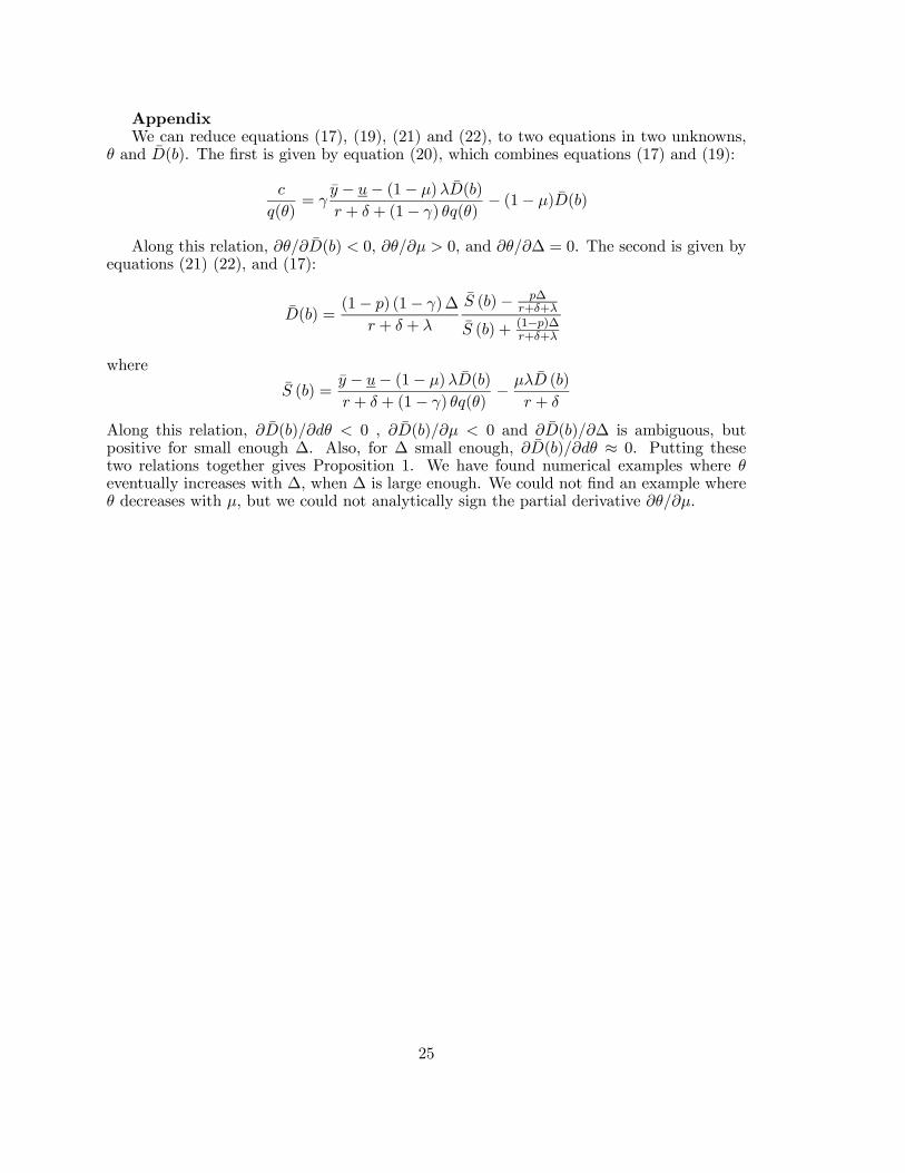
AppendixWe can reduce equations (17), (19), (21) and (22), to two equations in two unknowns,

θ and D(b). The first is given by equation (20), which combines equations (17) and (19):

c

q(θ)= γ

y − u− (1− μ)λD(b)

r + δ + (1− γ) θq(θ)− (1− μ)D(b)

Along this relation, ∂θ/∂D(b) < 0, ∂θ/∂μ > 0, and ∂θ/∂∆ = 0. The second is given byequations (21) (22), and (17):

D(b) =(1− p) (1− γ)∆

r + δ + λ

S (b)− p∆r+δ+λ

S (b) + (1−p)∆r+δ+λ

where

S (b) =y − u− (1− μ)λD(b)

r + δ + (1− γ) θq(θ)− μλD (b)

r + δ

Along this relation, ∂D(b)/∂dθ < 0 , ∂D(b)/∂μ < 0 and ∂D(b)/∂∆ is ambiguous, butpositive for small enough ∆. Also, for ∆ small enough, ∂D(b)/∂dθ ≈ 0. Putting thesetwo relations together gives Proposition 1. We have found numerical examples where θeventually increases with ∆, when ∆ is large enough. We could not find an example whereθ decreases with μ, but we could not analytically sign the partial derivative ∂θ/∂μ.

25

(i) (ii) (iii) (iv) (v)

OLS OLS OLS IV IV

Labor Relation in 1999 -0.025 -0.021 -0.026 -0.025 -0.028

-4.85 -2.63 -4.96 -3.83 -3.36

Union Density 0

0.7

Union Coverage -0.013

-0.77

Replacement Rate 0

0.3

Benefit Duration 0.004

0.94

Employment Protection 0.001

0.85

Active Labor Market Policies 0

0.77

Tax Wedge 0.001

1.49

Strength of Union 0.006

1.04

N 21 20 21 18 15

R2 0.553 0.647 0.578 0.509 0.558

Table 1: Labor Relations and Unemployment

Notes: The dependent variable is the unemployment rate in 2000, computed with data from the OECD. In (iv), labor relations are instrumented by workers involved and days lost to strikes over employment from 1961 to 1967. In (v), labor relations are instrumented by the attitude of the State towards early unions in the 19th century, as defined by Crouch (1993). Coefficients are in bold, t-statistics are below the coefficients.

AUS

AUT

BEL CAN

DNK

ESP

FINFRA

GER

GRE

IRL

ITA

JPN

NLD

NOR

NZL

PRT

SWE

SWI

UK

USA

.02

.04

.06

.08

.1.1

2U

nem

ploy

men

t Rat

e in

200

0

3 4 5 6 7Quality of Labor Relations in 1999

Figure 1. Unemployment Rates and Labor Relations

AUS

AUT

BEL

CAN

DNK

FIN

FRA

GER IRL

ITA

JPN

NLDNOR

NZL

SWE

SWI

UK

USA

34

56

7Q

ualit

y of

Lab

or R

elat

ions

in 1

999

-.5 0 .5 1 1.5 2Index of Labor Conflicts in the 1960s

Figure 2. Current Labor Relations and Past Labor Conflits

0.0

5.1

.15

Mea

n U

nem

ploy

men

t Rat

e

1960 1970 1980 1990 2000 2010

Hostile Neutral Cooperative

Countries Sorted according to Labor Relations in 19th CenturyFigure 3. Unemployments Rates

050

010

0015

00D

ays

Lost

per

Tha

usen

d E

mpl

oyee

s

1960 1970 1980 1990 2000 2010

Hostile Neutral Cooperative

Countries Sorted according to Labor Relations in 19th CenturyFigure 4. Strike Rates

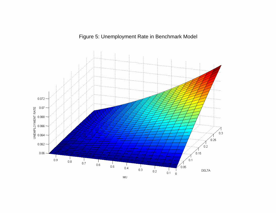
Figure 5: Unemployment Rate in Benchmark Model