The Quality of Growth: Fiscal Policies for Better...
135
IEG Working Paper 2008/6 The Quality of Growth: Fiscal Policies for Better Results Ramón E. López, Vinod Thomas, and Yan Wang This paper is available upon request from IEG-World Bank. 2008 The World Bank Washington, D.C. Public Disclosure Authorized Public Disclosure Authorized Public Disclosure Authorized Public Disclosure Authorized Public Disclosure Authorized Public Disclosure Authorized Public Disclosure Authorized Public Disclosure Authorized
Transcript of The Quality of Growth: Fiscal Policies for Better...
IEG Working Paper 2008/6
The Quality of Growth: Fiscal Policies for Better Results Ramón E. López, Vinod Thomas, and Yan Wang
This paper is available upon request from IEG-World Bank.
2008 The World Bank
Washington, D.C.
Pub
lic D
iscl
osur
e A
utho
rized
Pub
lic D
iscl
osur
e A
utho
rized
Pub
lic D
iscl
osur
e A
utho
rized
Pub
lic D
iscl
osur
e A
utho
rized
Pub
lic D
iscl
osur
e A
utho
rized
Pub
lic D
iscl
osur
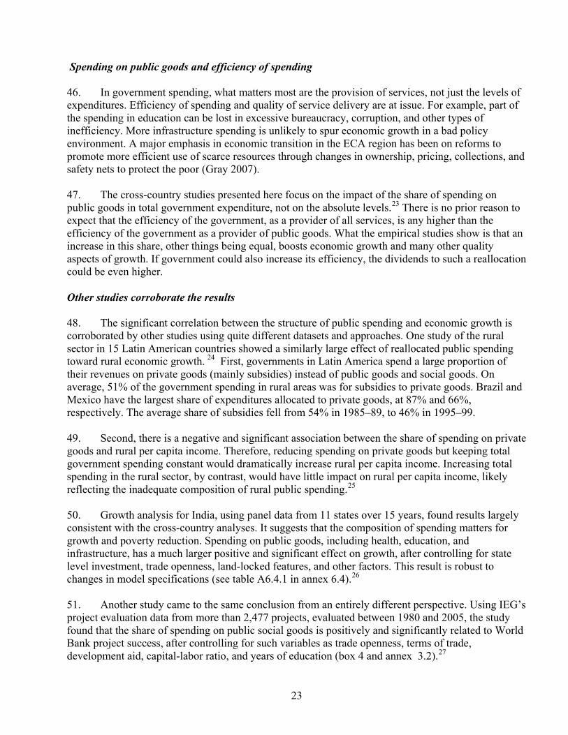
e A
utho
rized
Pub
lic D
iscl
osur
e A
utho
rized
Pub
lic D
iscl
osur
e A
utho
rized
wb370910
Typewritten Text
59625

ENHANCING DEVELOPMENT EFFECTIVENESS THROUGH EXCELLENCE AND INDEPENDENCE IN EVALUATION The Independent Evaluation Group is an independent unit within the World Bank Group; it reports directly to the Bank’s Board of Executive Directors. IEG assesses what works, and what does not; how a borrower plans to run and maintain a project; and the lasting contribution of the Bank to a country’s overall development. The goals of evaluation are to learn from experience, to provide an objective basis for assessing the results of the Bank’s work, and to provide accountability in the achievement of its objectives. It also improves Bank work by identifying and disseminating the lessons learned from experience and by framing recommendations drawn from evaluation findings. IEG Working Papers are an informal series to disseminate the findings of work in progress to encourage the exchange of ideas about development effectiveness through evaluation. The findings, interpretations, and conclusions expressed here are those of the author(s) and do not necessarily reflect the views of the Board of Executive Directors of the World Bank or the governments they represent, or IEG management. The World Bank cannot guarantee the accuracy of the data included in this work. The boundaries, colors, denominations, and other information shown on any map in this work do not imply on the part of the World Bank any judgment of the legal status of any territory or the endorsement or acceptance of such boundaries. ISBN-10: 1-60244-095-6 ISBN-13: 978-1-60244-095-1 Contact: Knowledge Programs and Evaluation Capacity Development Group (IEGKE) e-mail: [email protected] Telephone: 202-458-4497 Facsimile: 202-522-3125 http:/www.worldbank.org/ieg

1
Table of Contents
Abbreviations............................................................................................................................... 3
Acknowledgements...................................................................................................................... 4
Preface .......................................................................................................................................... 5
Executive Summary ..................................................................................................................... 6
1. How the quality of growth matters: Overview ...................................................................... 11
Quality of growth is a challenge in many parts of the world......................................... 12
2. Fiscal policies matter for the quality of growth: Framework ................................................ 16
3. Fiscal Policies matter for the quality of growth: Evidence.................................................... 20
Spending on public goods is associated with faster and better growth.......................... 20
Spending on public goods and efficiency of spending .................................................. 23
Other studies corroborate the results.............................................................................. 23
Fiscal policy has improved the quality of growth in some ways in some countries...... 25
…but not in other respects ............................................................................................. 27
4. Fiscal policy, poverty, and structural inequality.................................................................... 29
Growth, poverty, and inequality .................................................................................... 29
Spending on public goods is associated with poverty reduction ................................... 29
Taxation is non-progressive and unable to address inequality ...................................... 32
5. Fiscal policy and the environment ......................................................................................... 34
6. What all of this might mean for countries and donors........................................................... 39
Annexes
Annex 1 An Overview of Developing Country Performance in
the Quality Aspects of Growth ............................................................................. 41
Annex 2 A Conceptual Framework ..................................................................................... 44
Annex 3.1 Fiscal Policy and Economic Growth..................................................................... 51
Annex 3.2 Project Analysis: Composition of Public Expenditure Key
to Project Success ................................................................................................. 60
Annex 4 Fiscal Policy, Growth, and Income Distribution .................................................. 67
Annex 5 Fiscal Policy and the Environment ....................................................................... 78

2
Annex 6 Summary of the Country Studies ................................................................................ 86
6.1 Brazil and the Quality of Growth............................................................................................86 6.2 Chile and the Quality of Growth.............................................................................................91 6.3 Rebalancing China’s Growth..................................................................................................96 6.4 India: More and Better Growth and the Role of Fiscal Policy .............................................104 6.5 Twelve Fast-Growing African Countries..............................................................................111
List of Background Papers.......................................................................................................... 117
References ............................................................................................................................. 118
Endnotes...................................................................................................................................... 132
Tables and Boxes
Table 3.1 Spending on Public vs. Private Goods: Trends in Four Countries, 1985-2005 ........... 25 Table 4.1 Indirect Taxes as a Percentage of Total Tax Revenue................................................. 32 Box 1. Inadequate Attention to Inequality and the Environment .................................................15 Box 2. Brief Literature Review on Public Expenditures, Taxes, and Economic Growth.............19 Box 3. Key Empirical Results, Data, and Methodology Issues ....................................................21 Box 4. Analysis of IEG’s Project Ratings Supports the Cross-Country Results ..........................24 Box 5. Public Expenditure Reviews: Mexico (2004) and Indonesia (2007) ................................31 Box 6. Six Principles of Tax Reforms Proposed by the Hamilton Project in the US...................33 Box 7. Impact of the Environment on Public Health....................................................................34 Box 8. Fuel Subsidies Benefiting the Rich and Hurting the Environment ...................................36 Box 9. Impact of the Grain-for-Green Program in China.............................................................38

3
Abbreviations AFR Sub-Saharan Africa ARDE Annual Review of Development Effectiveness CAE Country Assistance Evaluation CAS Country Assistant Strategy CASCR Country Assistant Strategy Completion Report DALY Disability-adjusted life years EAP East Asia and the Pacific ECA Eastern Europe and Central Asia FY Fiscal year GEF Global Environment Facility HNP Health, Nutrition, and Population ICAO International Civil Aviation Organization ICR Implementation Completion and Results Report IEG Independent Evaluation Group IMF International Monetary Fund LCR Latin America and Caribbean LIC Low-income country LMIC Lower-middle-income country MAP Multicountry AIDS Program MNA Middle East and North Africa OED Operations Evaluation Department (now IEG) PPAR Project Performance Assessment Report SAR South Asia TSB Transport Sector Board UMIC Upper-middle-income country WHO World Health Organization

4
Acknowledgements As part of IEG’s work program, this technical report and the supporting background work were prepared by a team led by Professor Ramón E. López (University of Maryland) and Yan Wang (WBI), who task managed the paper. This paper and its related background work were conducted under the general guidance of Vinod Thomas (Director General, Evaluation), who also contributed to the paper. The report draws on work (listed in the annex), based on background technical studies by Ramón E. López, and country studies by Sadiq Ahmed (India), Bert Hofman and Louis Kuijis (China), Raj Nallari (Sub-Saharan Africa), Ramón E. López (Chile), Claudia Romano (Brazil), and Ann Elizabeth Flanagan (project analysis), with support from Houqi Hong, Asif Islam, Sebastian Miller, Máximo Torero, Sergio Sakurai, Shampa Sinha, and Bintao Wang. The team benefited at various stages in its work from advice and comments from Francisco H. G. Ferreira, Santiago Herrera, Brian Pinto, Martin Ravallion, Joanne Salop, and Zmarak Shalizi; and from Alan Barbu, Marvin Taylor-Dormond, Shahrokh Fardoust, Cheryl Gray, Ali Khadr, Nidhi Khattri, Keith MacKay, John Redwood, Mark Sundberg, Klaus Tilmes, Howard White, Dusan Vujovic, and other participants in the IEG review meeting. The task leaders gratefully acknowledge support and encouragement from WBI managers Roumeen Islam and Alex Fleming. The team is grateful for the advice and guidance provided by the peer reviewers for this work: Ken Chomitz, Luis Serven, Marcelo Selowsky, and Steven Webb. The team appreciates the assistance from Graciela Volterra Luna and Ritu Thomas. The summary report was edited by Bruce Ross-Larson, and annex was edited by Mellen Candage. Finally, the team is thankful to Shahrokh Fardoust (Senior Advisor) in IEG, who provided valuable advice throughout this effort.

5
Preface In a recent report on middle-income countries, Independent Evaluation Group (IEG) found that countries and the World Bank Group have been relatively effective in the overarching priority of promoting growth and reducing poverty, but not in addressing rising inequality, governance and corruption, and environmental degradation. Similar issues were raised in IEG’s 2006 Annual Report on Development Effectiveness (ARDE). Recent reports from the United Nations and other multilateral agencies such as the Asian Development Bank also document the concerns about these aspects of distribution and sustainability connected with growth. Following the analysis in The Quality of Growth (Thomas et al. 2000), this report takes “quality of growth” to mean the type of economic growth that especially reduces extreme poverty, narrows structural inequalities, protects the environment, and sustains the growth process itself. This is a challenging report on the development role of fiscal policy. It provides a multidimensional perspective on development—combining income growth, equity, and environmental quality. The report’s concerns are at the core of the development policy debate. The underlying analysis combines a variety of data and methodological approaches—from standard cross-country growth regressions to project data and country experiences. The report is intended to stimulate discussion in this critical area, particularly where the challenges from environmental and climate change problems, rising income inequality, energy subsidies in the face of rapidly rising energy prices, and widely uneven progress in combating poverty are becoming more serious. This paper—requested by the Committee for Development Effectiveness (CODE) and prepared as part of IEG’s work program—considers how fiscal policies affect the key dimensions of quality. There are three reasons why such a focus is crucial. First, the sustainability of development results is fundamentally affected by the nature of growth. Second, fiscal policies have an especially important effect on the quality aspects of growth, such as inequality and environmental sustainability. Third, this approach allows us to draw from previous work on projects, sectors, and countries, using evaluation data (such as the IEG database and recent IEG reports) and other data (cross-country), as well as to complement ongoing evaluation work on public sector reform, the environment, and climate change. The findings presented in this report should be useful for evaluating development results. In particular, those on the composition of spending and taxes could help in addressing the following questions:
• How have countries used fiscal policy (expenditures, subsidies, and taxes) to address inequality and environmental degradation, and how effective have they been?
• Which expenditures, subsidies, and taxes are best used to address inequality and to reduce resource depletion and emissions? Which subsidies should not to be used?
It is the authors’ hope that the findings from this work will lead to deeper consideration of both the quality and quantity dimensions of economic growth, especially in evaluations of development strategies and the resulting development effectiveness.

6
Executive Summary 1. The world faces unprecedented opportunities to reduce global poverty and improve human welfare. Strong global growth and better economic policies in recent years have substantially reduced poverty in many developing countries. However, with the recent financial turmoil in the United States and rising prices for food, oil, and other commodities, the world economy faces heightened risks and volatility. Policymakers around the world face the challenge of maintaining momentum in growth, as well as of improving the quality of growth. This concern over quality is reflected in the highly uneven reduction in poverty, rising inequality in numerous countries, and widening environmental degradation during the past decade—a period of unprecedented high economic growth in developing countries. Unless these issues are confronted, gains from growth are likely to be undermined and the pace of growth, itself, will not be sustained.
2. Growth is clearly linked to reductions in poverty. But the strength of this relationship depends on the quality or nature of growth. Various studies show that some growth patterns systematically reduce poverty and inequality, but others do not.1 And some growth patterns lead to underinvestment in human capital, overexploitation of natural resources, and degradation of the environment—patterns inimical to the sustainability of growth.
3. Following the analysis in The Quality of Growth (Thomas et al. 2000), we refer quality to aspects of growth that especially reduce extreme poverty, narrow structural inequalities, protect the environment, and sustain the growth process itself. Structural inequalities arise, inter alia, from imperfect markets (especially for credit) and from the privileges and transfers that states provide to special groups. Excluding some groups from opportunities to participate in productive activities represents an obstacle to creating wealth and improving human welfare.2 Although it is difficult to measure the quality of economic growth, this paper makes an attempt to do so by using multiple indicators, encompassing long-term growth (section 3), poverty and distribution (section 4), and six indicators of environmental pollution (section 5).
How fiscal policies matter for the pace and quality of growth
4. Fiscal policy is one of the most powerful instruments used by governments to maintain macroeconomic stability for growth, as well as for intra-generational and inter-generational transfers of wealth, and for correcting market failures. Governments often have at their disposal between 25% and 40% of national income for spending, including redistributions across social groups. The literature has studied the effects of trade policies, exchange rates, and the macroeconomic impacts of fiscal spending.3 However, it has been less focused on the allocative effects of government spending, taxes and subsidies on the pace and the quality aspects of growth, such as poverty/inequality and the environment. Few analysts have studied the impact of fiscal policy on the environment.4
5. The background work for this paper found that the composition of government spending matters for both the pace and the quality of growth. Here we differentiate between government spending on public goods versus private goods. Public goods are defined broadly to include expenditures that complement rather than substitute for production in the private economy. Where certain markets fail (e.g., credit markets imperfections, environmental externalities, and others) government expenditures targeted at mitigating the negative consequences of such failures are considered public goods. Among these are direct cash or in-kind transfers to financially distressed

7
households, as well as expenditures for basic education and health, social security, public infrastructure, institutional development, law and order, and others. Expenditures that provide spillover benefits, such as on basic research and on environmental protection and natural resource management—areas in which the private sector tends to underinvest5—also fall into this category. 6. Expenditures on private goods (production) or non-social subsidies include those that substitute for, rather than complement, production by the private sector. Often, these subsidies tend to distort markets; that is, unlike expenditures in public goods, they exacerbate market failures or create new distortions. Such subsidies include commodity subsidies (e.g., energy subsidies, agricultural subsidies) corporate subsidies, credit subsidies, credit guarantees, and many other ad-hoc schemes that are often targeted at special interest groups. Many investment subsidies, for example, are not across-the-board but, instead, discriminate in favor of certain industries or firms that are often selected on the basis of successful lobbying efforts. In general, subsidies for private goods—much more than expenditures for public goods—is the object of political lobbying, often involving relatively expensive and directly unproductive activities.
7. Government spending on pro-poor programs can reduce poverty, as in the conditional cash-transfer programs in Mexico, Brazil, Indonesia, and other countries. It can also provide such public goods as research and development infrastructure, basic education and health, and natural resource management—goods that the private sector would not provide. Fiscal policy, however, is deeply entrenched in the political economy, with subsidies and tax exemptions often captured by elites. So, despite their potential for promoting better quality growth, fiscal interventions, when misguided, can do more harm than good.
8. The empirical evidence presented here—cross-country and country case analyses, as well as project-level analysis—supports the idea that the composition of government spending and the institutional and governance setups in a country matter greatly for the quantity and quality aspects of economic growth. The following three findings are interrelated.
9. First, government spending on public goods is strongly associated with faster economic growth as well as with greater poverty reduction. , according to this report’s background work, including cross-country, country-level and project analyses. In other words, more spending on public goods (as broadly defined above) is linked to accelerated economic growth and reduced poverty. By contrast, government expenditures on private goods and on subsidies to firms that distort markets (e.g., energy subsidies), as opposed to public goods, are associated with weaker economic growth and greater structural inequality. Country and project studies corroborate this evidence (see box-table 3.1 and box 4). Therefore, reallocating government expenditures from private goods to public goods, even while keeping total government expenditure constant, could be associated with higher and better growth.
10. Second, government spending on public goods is also positively and significantly related to environmental quality. In general, a shift in the composition of government spending toward public goods, and away from private subsidies, is associated with improvements in the quality of the environment, as measured by air pollution indicators. This argues for reallocating government spending away from subsidizing the kinds of private goods that provide perverse incentives and lead to resource depletion, and toward providing more public goods.
11. There is a long way to go, though, before public goods are favored in fiscal policy. For example, the world spends a quarter of a trillion dollars a year on energy subsidies, thus providing incentives to waste energy, increase greenhouse gas emissions, accelerate climate change, and damage

8
human health. And the several hundred billion dollars spent on agricultural subsidies are captured mainly by a small subset of the wealthiest producers, thus reducing welfare in low-income countries. Similarly, water for agriculture is underpriced in most countries, and leads to greater waste of this resource. Globally, overuse of freshwater, estimated at 5% to 25%, is rapidly depleting the supply.
12. Third, the nature of tax policies also affects the quality of economic growth. The Latin American examples show how tax loopholes and evasion benefit mainly the well-to-do, and how dependence on indirect taxes increases the tax burden on poorer households. Taxation of natural resource rents is another important area requiring the attention of policy makers. For example, by failing to tax rents on natural resources, many countries miss an important source of tax revenues that causes little economic inefficiency. There is a heated debate on direct versus indirect taxation. Some argue that in many countries, corporate income-tax exemptions are provided to foreign investors in selected regions or sectors. Shifting some of the tax burden from indirect taxes to direct ones is therefore likely to not only improve equity but also to help reduce economic inefficiencies, given that such taxes tend to exacerbate the inefficiencies arising from credit market failure. Others have argued that indirect taxes may be less distortionary, as compared with labor and income taxes. Given that the existing empirical work has not yet provided conclusive results, this paper calls for a pragmatic approach, on a case-by-case basis, regarding the appropriate balance between direct and indirect taxes.
13. Tax policies need greater attention for addressing the pressing issues of environmental degradation. For example, taxing the rents of natural resources has received little attention, even though it is an efficient way of raising revenues. The Stern Review calls for price-driven instruments, such as carbon taxes and tradable quotas.6 Kyoto protocols provide a framework and Bali Summit provides a road map, and there has been progress on carbon trading, but the design issues regarding these carbon taxes and the political economy of implementation are far from being resolved. As countries are seeking greener fiscal policies, there is scope for more analysis and follow up on improved tax policy frameworks for sustainable development.
What all of this might mean for countries and donors
14. Few policy instruments can affect both the quantity and the quality of growth—fiscal policy can. Encompassing government expenditures, taxation, and subsidies, which all affect prices and disposable incomes, fiscal policy is perhaps the most contentious area of economic policy, heavily influenced by factors deeply seated in a country’s socio-political environment and institutions. This study is an initial attempt to shed light on a policy framework that countries might consider for improving their quality of growth.
• Restructuring government spending. This study confirms that government spending in public goods is associated with higher and better growth. In other words, more spending on public goods at the margin may be associated with accelerated growth, reduced poverty, and improved air quality. The expenditures could be restructured and transformed into effective instruments for reducing poverty, narrowing structural inequality, and promoting environmentally sustainability. To do so requires reallocating government spending away from subsidizing private goods that provide incentives leading to resource depletion, and toward providing more public goods, even while total government spending is kept constant, to ensure macroeconomic stability. This implies reducing perverse subsidies and reallocating public expenditures at the margin. It does not mean that government could select a growth trajectory that is not consistent with its comparative advantages. Structural inequality could be narrowed

9
by mitigating the effects of market imperfections and reducing the influence of interest group lobbies.
• Reforming tax systems. Plugging loopholes, reducing tax evasion, and fairly taxing rents from natural resources can make the tax system more efficient and less dependent on indirect taxes. Once public spending becomes more consistent with the objectives of economic growth, social equity, and the environment, the tax base could be broadened. New taxes and tradable quotas may be needed to establish the right prices for natural and environmental capital, thus generating more government revenue while providing the right incentives for reducing greenhouse gas emissions. Adequate taxation of rents from natural resources could be a priority. International coordination on tax systems is critical because capital flows easily across borders, and the international financial institutions can play a crucial role in standardizing tax codes.
• Providing public goods. With an increased revenue base, countries could then embark on a second round of providing more public goods, while ensuring fiscal sustainability. The second round could include more investment toward improving institutions and property rights, and reducing the impact of imperfect markets on efficiency and inequality. It could also include increasing the efficiency of government expenditures, which in turn would allow for raising the quality of education, health care, social protection, crime prevention, and infrastructure services. Other public goods include resource management, pollution control and abatement, and the adaptation of low-emission technologies.
15. The measures described above can be used for evaluating the effectiveness of financial and technical support provided by international financial institutions and other donors to developing countries:
• It would be valuable to conduct more analytical evaluations of government spending as part of the periodic reviews of public expenditure, particularly the split between spending on private subsidies and that on public goods. Incidence analyses on beneficiaries of private subsidies and of tax exemptions would also be useful as it is related to policy captures by higher income groups.
• There needs to be an increased emphasis on the evaluation of tax systems, particularly in documenting tax evasion and efforts to reduce them. Assess progress in eliminating tax loopholes, especially the most regressive ones, and in increasing the tax base to ensure fiscal sustainability, including studies of the impact of indirect taxation on economic efficiency.
• There is also a need to assess whether countries attain a fair share of the rents from natural resources and what countries are doing to reduce environmental degradation and enforce environmental regulations. It would be useful to provide more analysis on the best practices on greener tax and other fiscal policies for environmental sustainability.
16. The remainder of this report follows: section 1 provides an overview of the quality aspects of growth; section 2 provides a conceptual framework for the analysis; section 3 presents the key evidence that fiscal policy matters for faster and better growth; section 4 discusses the linkage between

10
the composition of taxes and expenditures, on the one hand, and poverty and income inequality, on the other; section 5 presents the results on fiscal policy and the environment, and section 6 gives the conclusions.. To improve readability, the empirical results from the cross-country analyses, country case studies, and a project-level analysis (based on IEG databases) have been summarized and are presented in the annexes to this paper.

11
1. How the quality of growth matters: Overview 17. Economic growth is positively related to poverty reduction and many attributes of human well-being. But experience shows that some growth patterns reduce poverty more effectively than others.7 And some growth patterns lead to overexploitation of natural resources and environmental degradation. Constructing indices for human development and for environmental quality, based on data from 128 countries, we see that per capita income growth is positively related to human development, but negatively related to the environmental quality, while controlling for initial income per capita (figure 1.1 and annex 1). Figure 1.1 Growth, human development, and environmental quality
Note: The authors constructed composite indices of human development and environmental quality based on data from 128 countries in the World Bank’s Global Development Finance and World Development Indicators central database for 2007. The relationships shown here control for the initial GDP per capita. See annex 1 for indicators and method used to construct the two indices. 18. Both pace and quality of growth are crucial to better development results. The Quality of Growth (Thomas et al. 2000) laid out the more pertinent quality aspects of growth: as poverty is reduced, social equity increases, environmental degradation stops, and growth is sustained.8 Describing the interrelationships among human capital, physical and financial capital, and natural and environmental capital, balanced investments in all three assets is seen to be essential for ensuring faster and better growth. Underinvestment in human capital and overexploitation of natural capital are seen to be harmful to the quality of growth. 19. Studies have shown that the patterns of growth matter for poverty reduction.9 Despite the centrality of the quality of growth, inadequate attention has been paid to equity and environmental sustainability (see box 1). Country success is almost exclusively defined by the rate of economic growth and growth policies. What is needed is an integrated approach measuring and linking the dimensions of growth. Correctly measuring GDP using “green” accounting and national wealth is an effort in the right direction, but operational applications must follow. 20. This paper explores the linkages between fiscal policy and the quality of growth. This paper takes ”quality” to refer to the type of economic growth that reduces extreme poverty, narrows
y = 0.0733+ 7.757x (t=5.48)
R2 = 0.1923
-80
-60
-40
-20
0
20
40
60
80
-7 -5 -3 -1 1 3 5 7 9
GDP growth not explained by initial GDP per capita
Cha
nge
in H
uman
Dev
elop
men
t Ind
ex n
ot
expl
aine
d by
initi
al in
com
e
y = - 0.2235-2.4766x (t=-2.45)
R2 = 0.0659
-50
-40
-30
-20
-10
0
10
20
30
40
50
-8 -6 -4 -2 0 2 4 6 8
GDP growth not explained by initial GDP per capita
Cha
nge
in E
nviro
nmen
tal q
ualit
y (b
row
n is
sues
in
dex)
not
exp
lain
ed b
y in
itial
inco
me

12
structural inequality, protects the environment, and hence sustains growth process itself. Consistent with the World Bank’s WDR on equity and development, we focus on structural inequality, which originates in the imperfections of markets and of government policy failures which often excludes low income groups from obtaining basic education and healthcare, and from participating in economic opportunities. High-quality growth requires narrowing structural inequality, but not necessarily reducing non-structural inequality, which can often be part of the market incentives to investment and growth. 21. Demand for high-quality growth is strong. In China, after decades of rapid growth and poverty reduction, the quality of China’s growth is now considered more important than its speed. In 2007, Chinese Premier Wen Jiabao labeled the economy “unstable, unbalanced, uncoordinated, and unsustainable.” As regional income disparities have widened and income inequality has worsened, the leadership has adopted several fiscal policy measures to achieve more balanced, inclusive, and sustainable growth.10 On March 18 2008, Wen Jiabao vowed, once again, to reform the fiscal and tax system to achieve “social fairness and justice” and to build “a people-centered” harmonious society. In India and Latin America, as well as several countries in Sub-Saharan Africa “jobless growth” has been at the center of public debates. In Chile, students took to the streets demanding better-quality education in 2006. Seeking high-quality growth is specified in the Vietnam Development Report and in its Five-Year Plan. Indonesia took decisive steps to reform its fuel subsidies in September 2005 and to compensate the poor by implementing a massive conditional cash-transfer system. 11 Quality of growth is a challenge in many parts of the world 22. Developing countries have had five consecutive years of fairly good economic growth, with average growth of 5.5% in 2004–06, excluding China and India. But huge challenges have arisen due to the sub-prime credit crisis in the US, which has led to a global economic downturn, and rising oil and food prices along with an increasing inflationary pressure. Long-term challenges remain: the varying pace of poverty reduction, the rising inequality, and the continuing environmental degradation. Twelve fast-growing African countries saw average annual growth of 4.3% in 1990–2006, others saw peaks and valleys, and still others did not grow at all. 23. Rapid growth has helped to achieve remarkable poverty reduction in many parts of the world, led by Asia. But there are large regional variations (figure 1.2). Inequality has risen in more than half of the middle-income countries, with Gini coefficients above 0.50 in many of them. In China, Lithuania, Sri Lanka, and Romania, and in several Latin American countries, the positive effect of growth on poverty was dampened by worsening income distribution. In some, where poverty increased, such as Bolivia and Georgia, negative household consumption growth was accompanied by an increase in inequality. While growth accounted for most of the poverty reduction, even seemingly small changes in income distribution contributed substantially to the poverty effects of growth.12 Meanwhile, carbon dioxide emissions are up in all regions, most notably in East Asia (figure 1.3).

13
Figure 1.2 Poverty reduction, by region Figure 1.3 Carbon dioxide emissions, by region
Source: World Bank main database. Note: These carbon dioxide emissions are those stemming from the burning of fossil fuels and the manufacturing of cement, and gas flaring. It does not include carbon dioxide from forest and agricultural emissions.
24. China achieved the fastest economic growth and poverty reduction in the last three decades. The current growth pattern relies heavily on manufacturing and external demand, and requires ever-increasing capital accumulation. On current trends, the ratio of investment to GDP would have to rise to more than 50% by 2020 and more than 55% by 2030 to achieve anticipated growth.13 The current growth pattern has also led to growing inequality. The accumulation of capital in urban industry widened productivity differences with rural areas, leading to large income inequalities. With an estimated Gini coefficient of more than 0.45, China is now less equal than the United States and Russia and on current trends is becoming more like Latin American countries (figure 1.4 and annex 6.3).
25. Although China has improved the use of natural resources and energy in some respects, environmental constraints on growth now loom large. As the second largest producer of carbon emissions, China has 16 of the 20 cities with the most polluted air. A recent World Bank study found that the health costs of air and water pollution in China amount to about 4.3% of its GDP. Adding the non-health impacts of pollution, estimated at about 1.5% of its GDP, brings the total cost of air and water pollution to about 5.8% of GDP.14
Poverty Headcount Index Percentage (of population living on less than PPP $1 per day)
0
10
20
30
40
50
60
East Asia &Pacific
Europe &Central Asia
Latin America& Caribbean
Middle East &North Africa
South Asia Sub-SaharanAfrica
Low & middleincome
19931996199920022004
Note: Based on 2000 purchasing parity rates. Poverty is defined as income of less than US$1 a
Carban Dioxide Emissions (billion tons)
0
1
2
3
4
5
6
East Asia &Pacific
Europe & CentralAsia
Latin America &Caribbean
Middle East &North Africa
South Asia Sub-SaharanAfrica
19921995199820012003

14
Figure 1.4 Income inequality is declining in Brazil and rising rapidly in China
Source: Papers by Romano and Sakurai annex 6.1, and Hofman and Kuijs (2007) (annex 6.3). 26. In Brazil, even with a low and volatile growth rate in the past decade, there has been a reduction in inequality. The country’s Gini coefficient declined from 0.59 in the late 1990s to 0.56 in 2005, due in part to social programs and tax reforms. One of the main environmental problems is deforestation. Deforestation rates in the Amazon have remained very high over the last decade and have shown significant annual fluctuations. Deforestation and land use changes account for 75% of Brazil’s carbon emissions. Air pollution, poor drinking water, and other environmental risks cause an estimated 233,000 premature deaths each year.15 27. In India, rapid growth since the 1980s has placed it among the top nine rapidly growing countries in the world, but the pace of poverty reduction has been slow. Income inequality increased between 1980 and 2004, and human development indicators remain weak, by international standards. India's particular problem is its low employment elasticity of growth, which has been narrowly based on high-tech and skill-intensive sectors. There are widening wage differentials between sectors and genders. Moreover, a growing population, rapid urbanization, and growth have all taken a toll on India’s natural environment. The estimated cost of environmental degradation is 5.8% of GNP—four times the 1.4% for high-income countries.(See annex 6.4 and the background paper by Sadiq Ahmed)16 Air pollution, contaminated drinking water, and other environmental risks cause an estimated 2.6 million premature deaths a year.17 28. Africa’s recent growth is associated with varying rates of poverty reduction and changes in inequality. Poverty levels dropped in Burkina Faso during 1990–2000, in Ghana and Kenya during 2000–05, and in Madagascar during the early 1990s. (However, levels have increased in Madagascar in the past few years because of negligible per capita income growth and an increase in income inequality.) A simple correlation analysis shows that growth in these countries is positively associated with poverty reduction—and with income inequality. Inequality worsened significantly in Uganda, owing partly to the slow growth in agriculture, and partly to inadequate job generation in other sectors. (See annex 6.5 and the background paper by Raj Nallari.)18
Brazil’s Gini coefficient China’s Gini coefficient
52
54
56
58
60
62
6419
81
1983
1985
1987
1989
1991
1993
1995
1997
1999
2001
2003
Without adjustments for spatial cost of
living differences
Adjusted for spatial cost of
living differences
45.3
41.1
20
30
40
50
1980
1982
1984
1986
1988
1990
1992
1994
1996
1998
2000
2002
2004

15
Box 1. Inadequate Attention to Inequality and the Environment Recent IEG reports found that inadequate attention was paid to equitable and sustainable growth. “Strategies designed solely to boost overall growth may miss opportunities to reduce poverty more effectively. In the countries reviewed by IEG, where growth did not result in poverty reduction, growth was concentrated in sub-sectors with low labor intensity and where few of the poor could work.” “The Bank has found it challenging to help countries formulate and implement strategies that effectively reduce rural poverty.” (World Bank-IEG 2007a, page xii). Income inequality is a pronounced and worsening problem in some middle-income countries (MICs). There are 18 MICs—all in Africa and Latin America—with Gini coefficients higher than 0.50, well above the global average. In more than half of MICs, inequality has worsened over the past decade. Bank publications, including the World Development Report 2006 and the regional report, Inequality in Latin America and the Caribbean (World Bank 2003b), have highlighted this issue. Yet, while many country assistance strategies show awareness of the topic and indicate that the Bank’s work will pay attention to the problem, the Bank has not yet succeeded in helping those clients deal with the problem convincingly (World Bank–IEG 2007a). Even in high-growth countries like China, “the Bank’s programs (fiscal 1993–2002) did not do enough to address inequality” (World Bank-IEG 2007b, p.25). And policy dialogues on fiscal decentralization issues have not been entirely effective. “The Bank has been less successful in persuading the government of the implications of broader development policies for poverty and inequality. The mismatch between intergovernmental fiscal resources and responsibilities has exacerbated regional inequality” (World Bank-IEG 2007b, p.9). When governments in poor regions were forced to provide fewer and lower-quality social services due to inadequate fiscal transfers, and passed along a higher proportion of the cost to their constituents, the outcomes were regressive (World Bank 2003c). In India, the Bank supported the reforms of the early 1990s. And in the late 1990s it sharpened its focus on poverty reduction and governance. “Overall, however, the Bank had limited impact on fiscal and other structural reforms and failed to develop an effective assistance strategy for rural poverty reduction through much of the 1990s” (World Bank-IEG 2007b, p.9). On the environment, high-income countries remain the largest emitters of carbon dioxide, but three-quarters of MICs have increased their emissions since 1995, including China, the world’s second-largest emitter. MICs account for nearly 60 percent of the world’s forest area, and four of 10 MICs have experienced deforestation since 1990; among them are Brazil, Indonesia, Mexico, and the Philippines. Bank lending for projects mapped to the Environment Sector Board in MICs has risen, but these projects have performed less well than projects in other sectors. Nearly one-third of such projects—with combined commitments of $892 million—had outcomes that were moderately unsatisfactory or lower, making it the worst-performing sector by a large margin (World Bank-IEG 2007b).

16
2. Fiscal policies matter for the quality of growth: Framework 29. This study builds in part on the framework found in The Quality of Growth (Thomas et al. 2000). A country has at least three types of assets that matter for production and welfare: physical capital, human capital, and natural capital. Technological progress and the policy environment affecting the use of these assets matter as well. Much attention has traditionally been given to the accumulation of physical and financial capital. However, for poverty reduction, what deserves greater attention are other key assets such as human (and social) capital, as well as natural (and environmental) capital, because these are primary assets that the poor possess.
30. Physical capital contributes to welfare through economic growth. Human (and social) capital and natural (and environmental) capital not only contribute to growth, they are direct components of welfare. Human capital and natural capital also help to increase investment returns, thereby attracting more capital and making the investment more productive. Accumulation of all three types of capital is crucial for a balanced and sustainable growth. 31. Market failures usually lead to underinvestment in human capital and overexploitation of natural capital. Such results affect the lower income segments of the population disproportionably and tend to benefit a minority of the population. Market failures are, therefore, a key source of structural inequality, which, in turn, is detrimental to efficiency and growth. In many countries, governments have failed to offset market failures by adequately providing basic services, especially to the poor. Since the benefits of investing in education and health take a long time to materialize, governments do not have sufficient political incentives to invest in the poor’s human capital. Instead, governments have contributed to structural inequality by using the scarce budget resources to subsidize and provide tax exemptions for often wealthy segments of the population. Figure 2.1 is a schematic illustration of this framework, showing the role of fiscal policy.
Figure 2.1 A framework for equitable and sustainable growth
Source: Based on The Quality of Growth, Thomas et al. 2000.
H(Humancapital)
Providing sound macro policy Opening to trade and investment Fiscal policies to provide correct
incentives to accumulate / use the 3 assets in a balanced way;
Correcting market failureshurting H and R
Good governance to ensure policyconsistency
R(Naturalcapital)
K(Physicalcapital)
WelfareEconomicGrowth
Tech. progress
Productivity growth
A Framework

17
Why the focus on fiscal policy? 32. First, fiscal policy is important for allocating resources to maintain a balance between the three key assets of the society: human capital, physical capital, and natural capital, which are critical for the quantity and quality of growth. The accumulation or depletion of these assets depends on the incentives created by tax policies and resources allocated through expenditure policies. Government expenditures often constitute more than 30% of GDP. Fiscal policy is therefore a powerful instrument, capable of affecting the orientation of asset accumulation and economic growth in dramatic ways. Second, fiscal policy is powerful enough to influence macroeconomic expansion and contraction and to affect intergenerational transfers through debt, social security, taxation on extractable resources and pollution, and subsidies and expenditures on mitigation and adaptation. 33. Third, fiscal policy is a weak link influencing global public goods or “bads” and assets and liabilities. It is also deeply entrenched in political economy and governance because subsidies and tax exemptions are often driven by the capture by elites. Therefore, despite their potential for promoting better quality of growth, the actual patterns could very well diverge and the outcomes of fiscal interventions may do more harm than good for quality of growth, in practice. For example, existing subsides (such as energy subsidies) often provide perverse incentives for resource extraction, depletion, and greenhouse gas emissions, leading to environmental degradation. 34. The framework for this study is related to three bodies of literature: (i) a large body of literature linking fiscal policy and long-run growth; (ii) the literature on the growth-poverty-inequality nexus; and (iii) a small but growing literature on taxes, subsidies and government expenditures, and the environment.19 Different types of government expenditures and different types of taxes may have very different effects on growth (Tanzi and Zee 1997). Several models have shown various mechanisms by which proper fiscal policies can be effective in promoting growth within an endogenous growth framework (Barro, 1990; Jones et al., 1993, Stokey and Rebelo, 1995). The allocation of public expenditures is likely to affect whether public expenditure is productive or not (Devarajan et al., 1996; Agénor and Neanidis, 2006). New growth theory stimulated studies that attempt to test the relationships between public expenditures and economic growth. Empirical evidence, however, on the relationship between composition of government expenditure and growth is neither conclusive nor robust. The distributional impact of tax loopholes and exemptions is largely ignored until recently (Furman, Summers and Bordoff 2007). (See box 2 for details.) Main hypothesis and taxonomy 35. This paper attempts to contribute to the literature by focusing on the linkages between fiscal policy and growth, poverty, inequality, and environmental sustainability. The main hypothesis is that the composition of fiscal expenditures matters for growth, for poverty reduction and inequality, as well as for environmental sustainability. An exogenous reallocation of government expenditures from private to public goods, if it can be sustained over time, promotes faster and more inclusive and sustainable growth. To guide our assessment, we developed a framework or taxonomy of government policies. For simplicity, we classify government policies into two types of interventions: A and B. (See annex 2 and López 2007 for a formal model). 36. Type A interventions emphasize using government expenditures to reduce the impact of market failure on the accumulation of assets, particularly human capital, knowledge, and the environment. These interventions are seen to be financed mainly through a reduction in expenditures,

18
such as non-social subsidies, that tend to exacerbate market failure. Type A interventions are thus likely to promote sustainable growth, based on balanced investments in physical, human, and natural capital. The emphasis on the provision of public goods by the state contributes to increasing the productivity of private investments. In addition, the focus of the public sector in providing environmental public goods promotes environmental sustainability. Finally, the reliance on social investments and other public goods, as well as avoiding inefficient and unnecessarily regressive taxation, tend to reduce the structural component of social inequality. Also, according to an increasing number of recent studies, structural inequality hurts economic growth. 37. Type B interventions focus on (non-social) subsidies to private goods, which are often captured by the elites. Subsidies to private goods, including commodity subsidies, credit subsidies, grants to corporations, loan guarantees, marketing subsidies, and others are much more easily appropriated by the most powerful interests groups, which are able to lobby governments most effectively. These type B programs trigger the lobbying activity in the private sector. Therefore, even if the objective of programs is to promote small enterprises, for example, they instead tend to be appropriated by the economically powerful. This, in turn, causes further structural inequality and more directly unproductive activities associated with rent-seeking. Finally, Type B interventions tend to distort markets when they are provided in the form of commodity market interventions (i.e., farm, energy, and water subsidies). 38. It is estimated that the total amount of support to agricultural and food sectors worldwide reached $499 billion in 2001 (25% of which was direct domestic and export subsidies and the rest was import tariffs), causing huge welfare losses in low-income agrarian economies (Anderson, Martin, and Valenzuela 2006, p. 362). Agricultural subsidies are especially captured by a small subset of wealthy producers and intermediaries that is able to spend large amounts of resources in lobbying government. Agricultural subsidies, therefore, increase economic inefficiency, contribute to increasing structural inequality, and induce more directly unproductive activity through rent seeking and crowding out of more productive expenditures from the government’s budget. In India, food and water subsidies benefit the rural rich (see background paper by Sadiq Ahmed and annex 6.4). In Africa, the rich benefit more from subsidies for fuel and kerosene. while “voice and accountability” mechanisms in the education sector can lower the capture of education subsidies by elites.20 39. The world spends a quarter of a trillion dollars a year on energy subsidies, which provide perverse incentives for wasting energy and increasing greenhouse gas emissions (Baig et al. 2007, Mati 2008; see box 8). In addition, such subsidies are an expensive and badly targeted at protecting the poor from rising energy prices; much of the benefits go to higher-income groups. The top 20 percent of households received, on average, about 42 percent of the total energy subsidy, whereas the bottom 20 percent received less than 10 percent (Coady et al., IMF 2006 and 2007). Moreover, by distorting price signals, non-social subsidies can lead to severe misallocation of resources. They also lead to inefficient investment choices, locking in energy infrastructure, and accelerating climate change. 40. Public and semi-public goods, as broadly defined above, are complementary with private investment because they tend to compensate for the scarcity of human and natural capital caused by market failure. Government’s provision of subsidies for private goods competes with the provision of public and semi-public goods due to limited or nonexistent fiscal resources. This crowding out of government expenditures in public and semi-public goods leads to underinvestment in human capital and natural capital. Underinvestment reduces the marginal productivity of private investments as the

19
private capital stock rises, thus increasing reliance on larger government subsidies to prevent the slowing down of growth. In this case, economic growth is based more on capital deepening than on productivity growth. Box 2. Brief Literature Review on Public Expenditures, Taxes, and Economic Growth A large body of literature explores the relationship between public finance policies and economic growth. Evidence can be found for a variety of different hypotheses, occasionally conflicting (see reviews by Perotti 2007 and Serven 2007). The most widely supported hypothesis is that public spending in two areas—education and infrastructure—is positively correlated with economic growth. Contradictory evidence also exists, however, in the case of infrastructure spending in developing countries. A recent study on public expenditure and growth has estimated the impact of volatility of government spending on consumption. The welfare loss due to the volatility of spending on consumption could be as large as 8 percent of consumption (Herrera 2007). Moreover, most literature to date has not considered the effect of governance on public spending outcomes (Gray 2007, p. 4). Aschauer (1989) found that spending on core infrastructure (streets, highways, airports, mass transit, and so forth) had a positive impact on private sector productivity. Several other studies have found positive growth effects of public investment (Nourzad and Vrieze 1995; Sanchez-Robles 1998; Kamps 2004), with some evidence supporting the law of diminishing returns (de la Fuente 1997). Furthermore, several studies found that public investment can be productive if it creates infrastructure that serves as input to private investment (Devarajan, Swaroop, and Zou 1996). The literature supports the growth-enhancing effects of expenditure on human capital if it is well targeted (Guellec and van Pottelsberghe 1999; Diamond 1999; de la Fuente and Domenech 2000; and Heitger 2001). Some studies, however, emphasized that public spending must complement, rather than crowd out, private spending (David, Hall, and Toole 2000). Consumption and social security spending have generally been found to have either no effect or a negative effect on growth (Aschauer 1989; Barrro 1990, 1991; Grier and Tullock 1989), although some (Cashin 1995) found a positive growth impact from welfare spending. For other categories of public spending, the evidence is even less conclusive. There has been a long-standing debate on the interaction between taxation and economic growth. Widmalm 2001, using a panel of 23 OECD countries, found that different taxes have different growth effects and that tax progressivity is bad for growth. The harmful effects of a progressive income tax structure were also noted by Padovano and Galli (2001, 2002), and Lee and Gordon (2005). The latter found that the marginal corporate tax rate was negatively correlated with economic growth in a cross-section of 70 countries during 1970–97, while other tax variables, including the average tax rate on labor income, are not significantly associated with economic growth. Kneller, Bleaney, and Gemmell (1999) found that an increase in productive expenditures enhances growth when financed by nondistorting taxation, provided the size of government remains relatively limited, while an increase in distorting taxes reduces growth. These studies, however, have not addressed the linkages between fiscal policy and structural inequality, or fiscal policy and the environment. The tax analyses have not distinguished between tax reductions that benefit all firms and tax exemptions that favor special-interest groups. A recent study by the Brookings Institution is an exception: Furman, Summers, and Bordoff (2007).point out that one of the reasons for the rising income inequality in the United States is related to tax exemptions and loopholes. __________________________ Source: Gray, Lane, and Varoudakis (2007); also cited in López and Miller (background paper 1), and López and Torero (background paper 2).

20
3. Fiscal policies matter for the quality of growth: Evidence 41. Cross-country, project-level analysis and country studies come together to support the idea that the composition of government spending and institutional and governance set-ups in a country matter for the level and quality aspects of growth. In this and following sections, we summarize the main findings of cross-country analyses linking government spending to growth, to poverty and inequality, and to the environment. Spending on public goods is associated with faster and better growth 42. This report’s cross-country analysis of 29 mostly middle-income countries, over 1980–2005, shows a large and significant positive relationship between government spending on public goods and economic growth, coupled with a mostly negative effect of total government spending on growth, when controlling for institutional, historical, governance, and geopolitical factors. This result is robust to changes in data, specifications, and estimation methods. So, a reallocation of government spending from (non-social) subsidies to public goods, while keeping total government expenditure constant, should be associated with faster growth. (annex 3.1)21 Such an effect is partly due to the reduction of non-social subsidies and partly to an increase in the share of public goods. 43. The estimated relationship between increasing the share of spending in public goods and growth is unusually robust to multiple sensitivity tests. Care has been taken to collect data and address the econometric methodological issues. A multiequation system approach was used to deal with the simultaneous interependencies and two-way links between these two variables. The three-stage least squares approach was used in the regressions (box-table 3.1), with institutional, political, geographic, and macroeconomic control variables. While the effect from the share of public goods to growth remains strong in all cases, the link between economic growth and share of public goods is weaker, and in some specifications, tend to be insignificantly different from zero, although always positive. This suggests that the causality most likely goes from public goods to growth. Sensitivity tests were conducted and results are robust—the share of spending on public goods remains positive and significant (see box 3). 22 44. What might lie behind this unusually strong correlation? Reallocating spending toward public goods seems to induce more balanced investment in human capital by reducing unproductive rent seeking and structural inequality. There are three benefits from doing so. 45. First, reallocation induces an increase in the rate of investment in human capital and knowledge by providing resources to households, which make these investments. A significant portion of households is financially constrained due to imperfections in credit markets that limit the investment in human capital. The increased financial resources available to households by increasing spending on public goods make the financial constraints on households less binding. Second, increasing government spending on public goods also means a faster rate of investment in infrastructure, knowledge diffusion, and the protection of natural resources. Finally, reducing the availability of government non-social subsidies reduces the incentives of the private sector to devote resources to unproductive rent-seeking activities and reduces commodity market distortions that curtail economic efficiency.
21
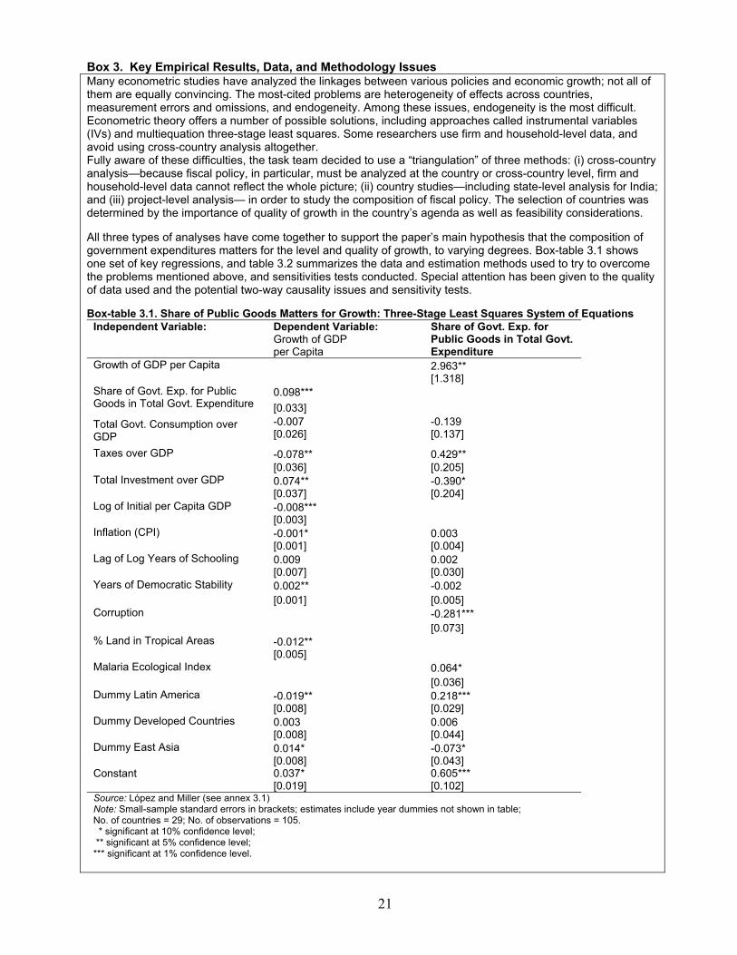
Box 3. Key Empirical Results, Data, and Methodology Issues Many econometric studies have analyzed the linkages between various policies and economic growth; not all of them are equally convincing. The most-cited problems are heterogeneity of effects across countries, measurement errors and omissions, and endogeneity. Among these issues, endogeneity is the most difficult. Econometric theory offers a number of possible solutions, including approaches called instrumental variables (IVs) and multiequation three-stage least squares. Some researchers use firm and household-level data, and avoid using cross-country analysis altogether. Fully aware of these difficulties, the task team decided to use a “triangulation” of three methods: (i) cross-country analysis—because fiscal policy, in particular, must be analyzed at the country or cross-country level, firm and household-level data cannot reflect the whole picture; (ii) country studies—including state-level analysis for India; and (iii) project-level analysis— in order to study the composition of fiscal policy. The selection of countries was determined by the importance of quality of growth in the country’s agenda as well as feasibility considerations. All three types of analyses have come together to support the paper’s main hypothesis that the composition of government expenditures matters for the level and quality of growth, to varying degrees. Box-table 3.1 shows one set of key regressions, and table 3.2 summarizes the data and estimation methods used to try to overcome the problems mentioned above, and sensitivities tests conducted. Special attention has been given to the quality of data used and the potential two-way causality issues and sensitivity tests. Box-table 3.1. Share of Public Goods Matters for Growth: Three-Stage Least Squares System of Equations
Independent Variable:
Dependent Variable: Growth of GDP per Capita
Share of Govt. Exp. for Public Goods in Total Govt. Expenditure
2.963** Growth of GDP per Capita [1.318] 0.098*** Share of Govt. Exp. for Public
Goods in Total Govt. Expenditure [0.033] -0.007 -0.139 Total Govt. Consumption over
GDP [0.026] [0.137]
-0.078** 0.429** Taxes over GDP [0.036] [0.205]
0.074** -0.390* Total Investment over GDP [0.037] [0.204]
-0.008*** Log of Initial per Capita GDP [0.003] -0.001* 0.003 Inflation (CPI) [0.001] [0.004] 0.009 0.002 Lag of Log Years of Schooling [0.007] [0.030] 0.002** -0.002 Years of Democratic Stability [0.001] [0.005] -0.281*** Corruption [0.073] -0.012** % Land in Tropical Areas [0.005] 0.064* Malaria Ecological Index [0.036] -0.019** 0.218*** Dummy Latin America [0.008] [0.029] 0.003 0.006 Dummy Developed Countries [0.008] [0.044] 0.014* -0.073* Dummy East Asia [0.008] [0.043] 0.037* 0.605*** Constant [0.019] [0.102]
Source: López and Miller (see annex 3.1) Note: Small-sample standard errors in brackets; estimates include year dummies not shown in table; No. of countries = 29; No. of observations = 105. * significant at 10% confidence level; ** significant at 5% confidence level; *** significant at 1% confidence level.

22
Box-table 3.2. Summary of Nine Background Studies: Data, Methods, and Sensitivity Tests Background paper #
Data Used Main Estimation Methods
Sensitivity Tests
1. Fiscal policy and growth (background paper 1, summarized in annex 3.1)
IMF Government Finance Statistics (GFS) data were complemented by data from ADB, country-level data and other data sources. See table A3.1.1.
Both multiequation three-stage least squares, and single-equation IV method are used.
A series of sensitivity tests, including bootstrapping—dropping one variable at a time, and dropping one country at a time. A sample dominance check was done (see figure 3.1.1 for bootstrapping results).
2. Fiscal policy and inequality (background paper 2, in annex 4)
40 countries: each country had at least two nationally representative household surveys during 1980–2005. The household income-distribution data from these surveys were combined with national accounts data, as well as other political and institutional data.
(a) SUR-IV estimates for the four-equation system (four income groups) presented in annex 4; and (b) based on estimated coefficients, parameters can be approximated from the variance-covariance matrix (tables A4.1-A4.4).
Same methods applied to the full country sample, and to poor and middle-income countries. Elasticities were calculated. Most results from the full sample are confirmed by the more disaggregated approaches. Both income and consumption were used as dependent variables and Wald tests were conducted.
3. Fiscal policy and the environment (background paper 3 in annex 5)
GEMS data containing 31 developing and developed countries with annual data for about 300 sites in 86 cities during 1985–2000, combined with government expenditure data from above.
Two-way fixed effects (TWFE) method controlling for site effects and common time effects (see table A5.2-A5.3).
Estimation results are robust using different methods, including OLS, RE, TWFE. Hausman tests were conducted.
4. Project analysis (box 4 and annex 3.2 )
IEG’s project evaluation data from more than 2,477 projects evaluated between 1980 and 2005. Two subperiods were used: the full sample period and post-1994 period.
Both logit and ordered logit were used for project-level analysis; instrumental variable for country-level analysis was employed for tests (tables A3.2.4 and 3.2.5).
To test for reverse causation and other endogeneity, an instrumental variable approach was employed following Dollar and Levine (2005). The key results remain robust.
5. Country study on India (see annex 6.4)
Expenditures at both levels of government: federal and state. In regressions, state level expenditure is used.
Instrumental variable and random effect (IV and RE), using state-level data.
Different model specifications were used and the key results remain robust (see tables A6.4.1-6.4.2).
Other country studies on Brazil, Chile, and China, and 12 African countries (annexes 6.1, 6.2, and 6.3, and 6.5)
Expenditure data used in figures include both levels of government: federal and state for Brazil, and general government for China. For Chile, data from budgetary central government is used.
No econometric analysis was done due to data difficulties.
N/A
Source: Based on background papers which are summarized in annexes. N/A = not applicable.
23
Spending on public goods and efficiency of spending 46. In government spending, what matters most are the provision of services, not just the levels of expenditures. Efficiency of spending and quality of service delivery are at issue. For example, part of the spending in education can be lost in excessive bureaucracy, corruption, and other types of inefficiency. More infrastructure spending is unlikely to spur economic growth in a bad policy environment. A major emphasis in economic transition in the ECA region has been on reforms to promote more efficient use of scarce resources through changes in ownership, pricing, collections, and safety nets to protect the poor (Gray 2007). 47. The cross-country studies presented here focus on the impact of the share of spending on public goods in total government expenditure, not on the absolute levels.23 There is no prior reason to expect that the efficiency of the government, as a provider of all services, is any higher than the efficiency of the government as a provider of public goods. What the empirical studies show is that an increase in this share, other things being equal, boosts economic growth and many other quality aspects of growth. If government could also increase its efficiency, the dividends to such a reallocation could be even higher. Other studies corroborate the results 48. The significant correlation between the structure of public spending and economic growth is corroborated by other studies using quite different datasets and approaches. One study of the rural sector in 15 Latin American countries showed a similarly large effect of reallocated public spending toward rural economic growth. 24 First, governments in Latin America spend a large proportion of their revenues on private goods (mainly subsidies) instead of public goods and social goods. On average, 51% of the government spending in rural areas was for subsidies to private goods. Brazil and Mexico have the largest share of expenditures allocated to private goods, at 87% and 66%, respectively. The average share of subsidies fell from 54% in 1985–89, to 46% in 1995–99. 49. Second, there is a negative and significant association between the share of spending on private goods and rural per capita income. Therefore, reducing spending on private goods but keeping total government spending constant would dramatically increase rural per capita income. Increasing total spending in the rural sector, by contrast, would have little impact on rural per capita income, likely reflecting the inadequate composition of rural public spending.25 50. Growth analysis for India, using panel data from 11 states over 15 years, found results largely consistent with the cross-country analyses. It suggests that the composition of spending matters for growth and poverty reduction. Spending on public goods, including health, education, and infrastructure, has a much larger positive and significant effect on growth, after controlling for state level investment, trade openness, land-locked features, and other factors. This result is robust to changes in model specifications (see table A6.4.1 in annex 6.4).26 51. Another study came to the same conclusion from an entirely different perspective. Using IEG’s project evaluation data from more than 2,477 projects, evaluated between 1980 and 2005, the study found that the share of spending on public social goods is positively and significantly related to World Bank project success, after controlling for such variables as trade openness, terms of trade, development aid, capital-labor ratio, and years of education (box 4 and annex 3.2).27
24
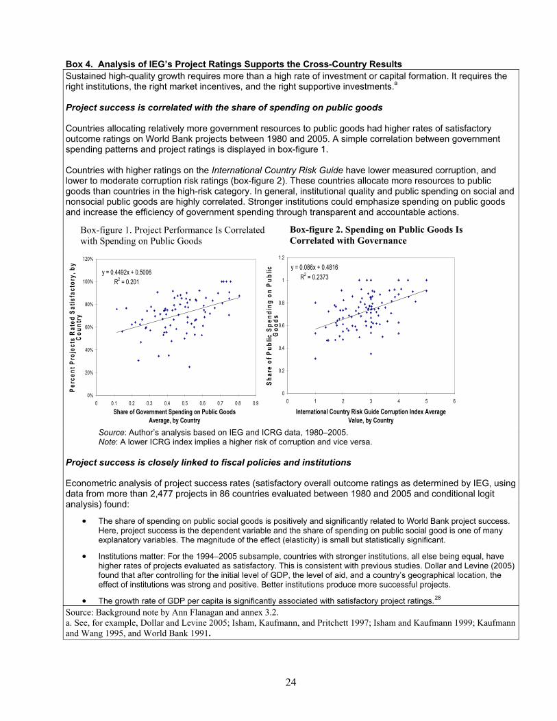
Box 4. Analysis of IEG’s Project Ratings Supports the Cross-Country Results Sustained high-quality growth requires more than a high rate of investment or capital formation. It requires the right institutions, the right market incentives, and the right supportive investments.a Project success is correlated with the share of spending on public goods Countries allocating relatively more government resources to public goods had higher rates of satisfactory outcome ratings on World Bank projects between 1980 and 2005. A simple correlation between government spending patterns and project ratings is displayed in box-figure 1. Countries with higher ratings on the International Country Risk Guide have lower measured corruption, and lower to moderate corruption risk ratings (box-figure 2). These countries allocate more resources to public goods than countries in the high-risk category. In general, institutional quality and public spending on social and nonsocial public goods are highly correlated. Stronger institutions could emphasize spending on public goods and increase the efficiency of government spending through transparent and accountable actions.
y = 0.4492x + 0.5006R2 = 0.201
0%
20%
40%
60%
80%
100%
120%
0 0.1 0.2 0.3 0.4 0.5 0.6 0.7 0.8 0.9
Share of Government Spending on Public GoodsAverage, by Country
Perc
ent P
roje
cts
Rat
ed S
atis
fact
ory,
by
Cou
ntr y
y = 0.086x + 0.4816R2 = 0.2373
0
0.2
0.4
0.6
0.8
1
1.2
0 1 2 3 4 5 6
International Country Risk Guide Corruption Index Average Value, by Country
Shar
e of
Pub
lic S
pend
ing
on P
ublic
G
oods
Source: Author’s analysis based on IEG and ICRG data, 1980–2005. Note: A lower ICRG index implies a higher risk of corruption and vice versa. Project success is closely linked to fiscal policies and institutions Econometric analysis of project success rates (satisfactory overall outcome ratings as determined by IEG, using data from more than 2,477 projects in 86 countries evaluated between 1980 and 2005 and conditional logit analysis) found:
• The share of spending on public social goods is positively and significantly related to World Bank project success. Here, project success is the dependent variable and the share of spending on public social good is one of many explanatory variables. The magnitude of the effect (elasticity) is small but statistically significant.
• Institutions matter: For the 1994–2005 subsample, countries with stronger institutions, all else being equal, have higher rates of projects evaluated as satisfactory. This is consistent with previous studies. Dollar and Levine (2005) found that after controlling for the initial level of GDP, the level of aid, and a country’s geographical location, the effect of institutions was strong and positive. Better institutions produce more successful projects.
• The growth rate of GDP per capita is significantly associated with satisfactory project ratings.28 Source: Background note by Ann Flanagan and annex 3.2. a. See, for example, Dollar and Levine 2005; Isham, Kaufmann, and Pritchett 1997; Isham and Kaufmann 1999; Kaufmann and Wang 1995, and World Bank 1991.
Box-figure 2. Spending on Public Goods Is Correlated with Governance
Box-figure 1. Project Performance Is Correlated with Spending on Public Goods

25
Fiscal policy has improved the quality of growth in some ways in some countries . . . 52. Several country studies illustrate the role of fiscal policies in changing the pattern of growth. Table 3.1 presents the shares of expenditure on public goods (type A) with that for private goods and subsidies (type B) in four countries over time. The share of type A expenditures has been high and rising in Chile and the share of type B has been declining. The ratios of type A to type B expenditures are rising in Chile and China for different reasons. In Chile there is a rapid shift to type A expenditure but, in China, the trend is associated with a reduction in type B expenditures over time as subsidies to state-owned enterprises declined during economic transition. (table 3.1). These ratios have remained nearly constant over time in Brazil and India. Comparisons need to be taken as illustrative and not definitive, given the weakness in the data, especially concerning type B expenditures. Table 3.1 Spending on public vs. private goods: Trends in four countries, 1985-2005
Brazil: Federal and state government expenditure 1985 1990 1995 2000 2004 2005 Average Share of public goods expenditures in total govt. expenditures 42% 30% 47% 35% 37% 38% 41% Share of private goods and subsidy in total govt. expenditures 24% 47% 36% 27% 32% 32% 34% Ratio of type A to type B expenditures 1.80 0.64 1.31 1.30 1.16 1.18 1.27 Chile: Central government expenditure 1985 1990 1995 2000 2004 2005 Average Share of public goods expenditures in total gov't expenditures n.a. 70% 78% 80% 82% 83% 77% Share of private goods expenditures in total gov't expenditures n.a. 30% 22% 20% 18% 17% 23% Ratio of type A over type B n.a. 2.32 3.55 4.03 4.70 4.83 3.58 China: General government expenditure 1985 1990 1995 2000 2004 2005 Average Share of public goods expenditures in total gov't expenditures 64% 60% 45% 50% 48% 48% 51% Share of private goods and subsidies in total gov't expenditures 34% 26% 17% 15% 14% 14% 21% Ratio of type A to type B 1.88 2.30 2.68 3.29 3.37 3.45 2.53 India: Consolidated general government 1985 1990 1995 2000 2004 2005 Average Share of Public goods expenditures/Total exp & Net lending 32% 31% 29% 29% 29% 32% 30% Share of Private goods expenditures/Total exp & Net lending 18% 18% 18% 18% 19% 18% 18% Ratio of type A to type B 1.77 1.71 1.63 1.62 1.49 1.82 1.63
Note: See paragraphs 36 and 37 in section 2 for definitions of types A and B. This table is illustrative because these ratios of type A to type B are calculated based on data from individual country studies from government sources. They are only comparable over time for each country, but not comparable across countries because definitions of private goods and subsidies (type B) may differ. See annexes 6.1, 6.2, 6.3, and 6.4 for sources. 53. In Chile, the government rationalized the expenditure side very well, with the share of spending on public goods rising to more than 71% in the early 2000s, one of the highest in the countries studied, starting from 55% in the early 1980s. Chile shows that a drastic reallocation of government spending can be done in a relatively short time span, despite heavy lobbying to protect subsidies (see table 3.1 and figure 3.1). This reallocation could be one of the reasons for Chile’s rapid growth over the last 15 years.29

26
Figure 3.1 Ranking of various types of expenditure: public goods vs. total Country Ranking by Share of Expenditure on Public Goods
01020304050607080
Cos
ta R
ica
Uru
guay
Chi
le
Pana
ma
Spai
n
Boliv
ia
Arge
ntin
a
Irela
nd
Mau
ritiu
s
Tuni
sia
Dom
inic
anR
epub
licJo
rdan
Chi
na /a
Col
ombi
a
Thai
land
Sing
apor
e
Gre
ece
Isra
el
Mex
ico
Egyp
t, Ar
abR
ep. Braz
il
Mal
aysi
a
Nep
al
Sri L
anka
Bang
lade
shKo
rea,
Rep
.In
dia
Philip
pine
s
Turk
ey
Indo
nesi
a
Perc
ent
Country Ranking by Total Govt. Expenditure over GDP Ratio
0102030405060
Jord
an
Indi
a
Sri L
anka
Isra
el
Chi
na /a
Braz
il
Nep
al
Chi
le
Indo
nesi
a
Mal
aysi
a
Uru
guay
Col
ombi
a
Boliv
ia
Cos
ta R
ica
Pana
ma
Arge
ntin
aD
omin
ican
Rep
ublic
Philip
pine
s
Thai
land
Spai
n
Irela
nd
Turk
ey
Gre
ece
Mex
ico
Tuni
sia
Mau
ritiu
sKo
rea,
Rep
.Eg
ypt,
Arab
Rep
.Ba
ngla
desh
Sing
apor
e
Perc
ent
Country Ranking by Investment over GDP Ratio
01020304050
Sin
gapo
reK
orea
,R
ep.
Thai
land
Chi
na /a
Mal
aysi
a
Isra
el
Spa
in
Gre
ece
Irela
nd
Chi
le
Mex
ico
Indo
nesi
a
Nep
al
Bra
zil
Pan
ama
Jord
an
Tuni
sia
Turk
ey
Arge
ntin
a
Phi
lippi
nes
Sri L
anka
Uru
guay
Col
ombi
aD
omin
ican
Rep
ublic
Mau
ritiu
s
Indi
a
Bang
lade
sh
Cos
ta R
ica
Bol
ivia
Egy
pt, A
rab
Rep
.
Perc
ent
Source: Based on data from cross-country analysis by López and Miller (Background paper 1 and annex 3.1). Note: China is added here based on the background paper on China (by Bert Hofman and Louis Kuijs, annex 6.3). 54. In China, the government mobilized public resources for massive investments—large dams, power generation systems, and national and regional highways. But it has been less successful in providing basic social services to rural and poor regions. Public spending on physical infrastructure has been among the highest in the world, which is good for growth. But the share of spending on education and health has been among the lowest. China is now reforming its transfers and subsidies (including cutting VAT tax refunds to resource-intensive exports) to promote more balanced growth.30 Subsidies to the state-owned enterprises have been gradually reduced, and preferential tax treatment to foreign investors is to be reformed and eliminated in 2008.31 A program of “returning cropland to forest” or Payment to Ecological Services (PES) has started to show positive results in both reforestation and in reducing rural poverty by encouraging rural-urban migration. 55. Brazil’s achievements in reducing poverty and inequality can be partly attributed to higher social spending and possibly to better tax collection. The incidence of poverty fell from 38% to 34.5% between 1995 and 2004. Inequality, as indicated by the Gini coefficient, fell from about 0.59 in the late 1990s to 0.56 in 2005.32 There was an increase in the share of spending on public goods from 32% in 2000 to 38% in 2005, but the share of type B spending has also increased (table 3.1). Recent studies suggest that social assistance can explain, at most, 50% of the reduction in inequality. A significant part of the remaining unexplained reduction in inequality could be because of higher tax revenue.

27
Increased government enforcement of tax collection, reduction of tax evasion, and lower income tax exemptions are likely reducing inequality. 56. Various studies show that income taxes are progressive in Brazil, so increasing taxes is likely to improve the income distribution. There has also been a parallel “pro-distribution” development: a gradual but steady decrease in income tax exemptions, from 0.56% of GDP in 1998 to 0.44% of GDP in 2005. Even if not large, this change has a positive effect on the distribution of income. Continuing to rely on indirect taxes has proven to be regressive.33 57. In Africa fiscal resources have increased since the Heavily Indebted Poor Countries (HIPC) initiative in the mid-1990s, and public spending on education, health, and water and sanitation rose significantly, improving human development indicators. Many challenges remain, however. Government revenue as a share of GDP, has remained flat for decades in each of the countries studied, at about 10–14% of GDP, despite several attempts to strengthen tax administrations. Revenue collection in other low-income countries is around 20% of GDP, and in developed countries it is 30–40% of GDP. Low revenue collection constrains the governments’ developmental role in improving the quality of life.34 . . . but not in other respects 58. Chile’s tax policies have not been on par with its expenditure policies. Tax loopholes have benefited mainly the rich. They amount to foregone revenues on the order of 5% of GDP, with about 81% of the benefits going to the wealthiest 5% of the population, and 61% to the richest 1% (table A6.2.1 in annex 6.2).35 Chile has not taxed the large resource rents, appropriated by a few domestic and foreign corporations, thus reducing the potential pro-poor effects of growth. The tax loopholes and the reluctance to tax the rents of natural resources significantly contribute to a narrowing of the tax base. These may be reasons why the country has not been able to extract an even higher growth dividend from its exemplary spending policy 59. China’s fiscal system is still in the transition process from the planning model of financing industrialization to the market model of providing public goods and services. Its fiscal stance has improved since the tax reform of 1994, with the fiscal envelope reaching nearly 25% of GDP, including extra-budgetary funds. Fiscal disparities among subnational governments are large. The richest province has more than eight times the per capita spending of the poorest provinces and the richest county has about 48 times more per capita spending than the poorest. 60. But China’s fiscal policy does little to redistribute income. The current transfer system is dominated by tax rebates and numerous earmarked grants, which together make up more than 60% of total grants. The general equalization grant makes up only 10% of transfers to the regions, leaving a mismatch between local government responsibilities and resources. Governments in poor regions therefore offer fewer (and lower quality) public services than their counterparts in rich regions. Income tax is rising but accounts for a small share in total government revenue, whereas, indirect taxes account for 72 percent of total tax revenue in 2005.36 61. India’s fiscal policy has not been very effective in reducing poverty or in managing the environment. Since the 1970s, India has run fairly large fiscal deficits (an average of 8% of GDP), building up a huge domestic public debt and large interest payment obligations. In 2004, the debt-to-GDP ratio reached almost 90%, and interest payments climbed over 7% of GDP, substantially

28
exceeding total public investment. The large fiscal deficits have not helped growth. And large interest payments and wage increases have constrained India's ability to invest in infrastructure and human development. 62. Each year India spends about 5% of GDP on subsidies, including that for food, fertilizer, petroleum products, and electricity. Many of the subsidies are aimed at helping the poor, but evidence suggests that the actual benefits are likely to have accrued more to the rich. For example, the electricity subsidy adds a huge financial burden to state government budgets, reduces investment, and leads to inefficient power use. Incidence analysis shows the targeting of this massive subsidy to be poor. Incidence analysis of health and education spending also suggests scope for substantially improving equity.37 63. In Ghana, public spending on infrastructure construction has increased since the early 1990s, facilitating trade, growth, and informal sector development. Access to electricity rose from 30% in 1991 to 50% by 2006, but only 10% of the electricity subsidies reached the poor. About 20% of the poor now have access to electricity, far less that the 56% for the non-poor. Poverty-related public spending has been high, at about 6% of GDP since 1992, but the pattern of public spending is heavily oriented toward the wage bill. Government employment is large, and wage awards to the public sector are frequent and large, especially around the time of national elections. This pattern of government spending did not benefit the poor as much as it could have.38

29
4. Fiscal policy, poverty, and structural inequality 64. The efficiency of translating economic growth into poverty reduction depends on the initial level of income, initial degree of income inequality, and whether growth is accompanied by changes in inequality.39 There is a vast literature on the growth-poverty-inequality nexus. The literature is conclusive on the first question of growth-poverty association. The empirical literature suggests that economic growth may affect inequality, but there is a significant variance when it comes to the relationship between public expenditure and inequality. These studies address three themes: (i) the relationships among measures of social capital, government actions, and inequality; (ii) the median-voter hypothesis and its implications for fiscal policy; and (iii) the effects on inequality of public spending (specifically education and health).40 Only a few studies have examined the impact of fiscal policy on poverty and inequality directly, due to poor data quality.41 Growth, poverty, and inequality 65. Our cross-country assessment makes clear the effect of fiscal policy and GDP growth on inequality and poverty.42 It uses a sample of 40 developing countries, with each country having had at least two national household surveys during 1980–2005. The household income-distribution data from these surveys were combined with national accounts data and other political and institutional data. The empirical method departs from the above studies in three ways. First, it measures the impact of public expenditures on the different parts of the distribution directly. Second, it looks at the composition of public expenditures, not just its aggregate level. Third, it studies the effects of public expenditures on the income growth rate (instead of income levels) of the various income groups. 66. This work confirms that GDP growth is good for the poor in middle-income and low-income countries (see annex 4). This is consistent with previous studies by Dollar and Kraay (2002), Ravallion and Chen (2004), and others. Our study did not find evidence of a growth and inequality tradeoff. It shows that GDP growth improves the distribution of income quite significantly in middle-income countries but not significantly in low-income countries. This is consistent with Ravallion’s work showing no evidence of tradeoff between growth and inequality.43 In Chinese provinces where growth and poverty reduction was rapid, inequality did not worsen. So, growth can be good for the poor and perhaps also for social equity, especially in the subsample of middle-income countries.
Spending on public goods is associated with poverty reduction 67. Our analysis also shows that reallocating government spending from private goods and non-social subsidies to public and semi-public goods, while keeping the total government expenditures constant, is associated with reductions in poverty. Government expenditures in social goods have a positive association with average household income and with the different groupings of household income, even though their distribution effect is neutral. The quantitative value of the effects of social expenditures on the household incomes in the poor countries is, however, rather modest. This implies that a reallocation of government spending to social public good will be associated with reducing poverty, but not income inequality.
68. Public social spending is distribution-neutral in our sample of low-income countries during 1980–2004, implying poor targeting. Despite many successes, such as the conditional cash transfer programs in Brazil, Mexico, and other countries, some pro-poor programs have not reached the intended beneficiaries. The fact that social spending is distribution-neutral, however, often implies that

30
the poor are at least sharing part of the benefits of social programs. But inefficiency of spending often stands in the way: in Uganda in the early 1990s, for example, only 13 percent of the public education grants were reaching the end-users or schools. Information provided to the public in local newspapers, about the transfer of public funds for primary schooling and expenditure-tracking exercises enabled Uganda to significantly reduce district-level capture of public funds by local elites (see annex 6.5).44
69. The India country study also corroborates these empirical results. State government spending on social public goods, including education and health, has a significantly positive association with poverty reduction and state GDP per capita, while inflation has a negative association. Reallocating spending to increase the share of social public goods could be associated with a significant reduction in the poverty headcount index during the sample period.45 These results are consistent with the findings from our cross-country reviews.
70. Spending on non-social subsidies tends to be well targeted and favors the wealthy, mainly because they have resources to finance rent-seeking investments. Spending on social goods, however, can benefit the poor with careful targeting. Direct transfers to households increase economic efficiency by allowing credit-constrained households to implement profitable investments. It is often politically difficult to reform subsidies that benefit the well-off, but adding new social subsidies to the poor is not difficult. The experiences of Mexico and Chile show that a shift in public expenditure patterns toward public goods can be done relatively quickly. Indonesia also reformed its fuel subsidies in a major way in September 2005, with limited success, although continued reform is needed (see box 5). Significant efforts must be devoted to the political economy of reforms: there is a need to balance the interests of the poor and the relatively well-off and to design a reform package (see Allcott, Lederman, and López 2006).
31
Box 5. Public Expenditure Reviews: Mexico (2004) and Indonesia (2007) The Bank conducts Public Expenditure Reviews (PERs) regularly. While earlier PERs focused more on the macroeconomic impact of fiscal policies, recent ones have moved to analyze the pro-poorness of public expenditures, linking composition of public expenditure with growth, poverty, and income distribution. The incidence of taxes (direct and indirect taxes) and incidence of tax loopholes and exemptions, however, have not been widely analyzed. Two important PERs have provided supporting evidence that the composition of spending matters. Mexico: The PER finds that Mexico’s public finance system is redistributive in its impact. Most resources are raised from taxation of richer households and states. And, on average, public spending provides comparable benefits per capita to households and states at various income levels. A total of one-third of central government spending goes for untargeted social programs with substantial participation by the poor, and almost 3 percent of central government spending goes for the poverty-targeted programs such as Oportunidades and Procampo. The report points to “powerful vested interests [that] have captured important parts of spending, which then become rigid expenditures that are difficult to reallocate to the government’s programmatic priorities.” Public investment has been low until recently, and the quality of services delivered is largely unknown, and perhaps inadequate and inequitable in important areas such as education. Mexico’s experience of the last decade is positive, however, showing that it is possible to reallocate resources away from inefficient but entrenched programs like general food and agricultural subsidies, toward more effective and pro-poor initiatives, such as Progresa/Oportunidades and Procampo, when they are well conceived and publicly presented (World Bank, Mexico PER 2004, and Webb 2004). Indonesia: The PER finds that macroeconomic policies with fiscal prudence have created a favorable environment for development results: the country now has sufficient fiscal space and financial resources to address its development needs. Thanks to fiscal decentralization in 2001, one-third of central government expenditure was transferred to the regions. Provincial and district governments now manage 37 percent of total public expenditures and carry out more than 50 percent of public expenditure. Spending on subsidies and administration, however, accounts for one-third of total expenditures. Subsidies in 2006 still consume roughly 15 percent of the total budget and remain at the 2004 level. Spending on public investment has recovered to the precrisis level of 7 percent, and spending on education has risen. However, health spending and public infrastructure investment have been low. The report points out that fuel and electricity subsidies are still a significant portion of the budget and largely benefit the better-off citizens. Although the 2005 adjustment to domestic fuel prices freed up US$10 billion, in 2006 Indonesia still spent US$12 billion on subsidies, particularly on fuel and electricity—both are regressive. Reducing and reallocating inefficient and pro-rich subsidies would free up additional fiscal resources of up to US$12 billion. In particular, electricity subsidies account for 28 percent of all subsidy cost, and largely benefit better-off Indonesians. Therefore, reducing subsidies for all electricity voltages above 450 volt-amperes should be pro-poor, since the higher voltage levels are used disproportionately by those who are better off (World Bank 2007). Source: World Bank 2004 for Mexico and World Bank 2007 for Indonesia. Note: The 2005 Fuel Price Adjustment, which doubled the gasoline price and tripled the kerosene price, was considered “one of the most significant policy reforms of any developing country in 2005” (World Bank). Subsequent studies have summarized the experiences and implications for other countries (Granado, Agustina, Bulman, Fengler, and Ikhsan 2008).

32
Taxation is non-progressive and unable to address inequality 71. Our cross-country analysis suggests some evidence that taxes, as they are currently implemented, are non-progressive within the household sector. These results are consistent with recent studies such as Lopez and Serven (2007) in that not much can be expected in terms of redistribution via taxation. The main reasons behind our results seem to be associated with the heavy reliance on indirect taxes, loopholes benefiting the wealthy and rampant tax evasion, which also mainly benefit the rich. These underlying factors are better explained by the country studies, and other recent evidence presented in studies by the Brookings Institution, Inter-American Development Bank, IMF, and World Bank.
72. Indirect taxes. There is greater reliance on indirect taxes than on resource rents, income taxes and property taxes. Table 4.1 presents the share of indirect taxes in total tax revenue for four countries. This table is only illustrative, because it is based on data from country case studies for which the definitions may vary. Some economists consider indirect taxes to be regressive while others consider them to be less distortionary, as compared with labor and income taxes. The World Development Report 2006 pointed out the need to “keep indirect taxes from being regressive. With a few key exemptions, the VAT can be made less regressive. Bird and Miller (1989) show that in Jamaica, exempting five specific items from VAT halves the burden on the poorest 40% of population.”46 An IMF staff paper found that “replacing sales taxes with a comprehensive VAT typically makes indirect taxes less progressive,” implying that lower-income households are likely to be net losers from revenue-neutral reforms. Studies also show that the progressiveness of the VAT can be improved by zero-rating certain categories, such as basic foods.47 A balanced approach between direct and indirect taxes (implying a 50:50 ratio) may be a feasible option to consider, pending further investigation, as the public finance literature does not provide a conclusive answer.
Table 4.1 Indirect Taxes as a Percentage of Total Tax Revenue Country 2004-05 Brazil 51.4 Chile 68.0 China* 72.0* India 51.2 OECD Average 32.0
Note: This table is only illustrative, because data are based on country studies. *China’s tax system is still in transition. There are 5 types of indirect taxes in China: VAT (tax rate at 17 percent; but basic necessities and agricultural products and utility are taxed at 13 percent; and exports of goods at zero rate) accounts for 36 percent of total tax revenue; consumption tax (14 categories of goods) accounts for 5 percent of tax revenue, and business tax accounts for 14 percent of tax revenue, in addition to a tax on imports (14 percent) and tariffs (3 percent), and others. (For details, see KPMG’s Corporate and Indirect Tax Rate Survey 2007, and China Statistical Yearbook 2006, p. 287).
73. Some evidence from Brazil shows that while its direct taxes are progressive, indirect taxes are regressive. Adding them together, the total tax burden for households would be regressive: In 2004, families earning up to two times the minimum wage had a total tax burden of 49% of their family income, while the richer households had a total tax burden of 26% (table A6.1.1 in annex 6.1). In Chile, a resource-rich country, failing to tax resource rents distorts incentives in favor of the resource industries, thus exacerbating the dependence on natural resources for income generation.48
74. Tax loopholes. There are legal tax loopholes which mainly benefit the rich segment of the population. In Chile, according to a recent report by the internal tax office, the loopholes account for almost 5% of GDP, with 61% of them benefiting the richest 1% of the population. The distributional impact of tax loopholes has not been carefully investigated. Also, due to the mainly discretionary
33
nature of these loopholes, there is a presumption that they cause economic inefficiency, but there are few studies showing the extent of this effect. While reducing taxes on profits may, under certain conditions, be advisable as a measure to promote investments, doing so by allowing for special tax loopholes instead of across-the-board reductions in the profit tax rate is not likely to cause such an effect. A recent study of the US tax system links tax loopholes with the rising inequality (Furman, Summers, and Bordoff 2007).
Box 6. Six Principles of Tax Reforms Proposed by the Hamilton Project in the US In a strategy paper of the Hamilton Project, Furman, Summers, and Bordoff (2007) point out that, “Taxes contribute, as part of the problem or as part of the solution, to many of the challenges our nation faces. The present tax treatment of health insurance, for example, pushes health spending upward while offering many of the uninsured little help in getting coverage. The tax treatment of retirement savings provides a windfall for high-income Americans who would likely have saved anyway, while offering scant encouragement to saving by low- and moderate-income Americans. America’s factories and cars continue to emit vast amounts of the carbon dioxide that drives climate change, a problem that would be remedied, in part, if the tax code imposed a cost for burning carbon-emitting fossil fuels.” (p. 3). The authors then present six principles of tax reforms: 1) Fiscal responsibility requires addressing both taxes and spending.
2) Rising inequality strengthens the case for progressivity. 3) The tax system should collect the taxes that are owed. 4) The tax system should strengthen taxation at the business level. 5) Taxes for individuals should be simplified. 6) Social policy can and should often be advanced through the tax code and it must be well designed.
“Tax policy can affect outcomes not just by subsidizing desirable activities but also by penalizing undesirable ones. In this manner, so-called Pigouvian taxes can lead business and consumers to take the social costs of their actions into account, helping to ensure that the outcome of market competition is efficient. Today, for example, gasoline taxes fall short of neutralizing the external harm associated with gasoline consumption, which includes not only climate change but also congestion, traffic accidents, and increased economic vulnerability to supply disruptions. Meanwhile the production of electricity and other energy from coal and natural gas is not taxed at all, despite its large contribution to climate change.” (p. 26.) On the political economy of reforms, “a forthcoming Hamilton Project discussion paper will show how carbon taxes to address these issues could be combined with other tax cuts to keep the outcome revenue neutral and distributionally neutral, thus protecting low and moderate-income families who would otherwise have a hard time paying the higher bills.” (p. 26.)
Source: Furman, Summers, and Bordoff 2007. “Achieving Progressive Tax Reform in an Increasingly Global Economy.” Brookings Institution.
75. Tax evasion. With evasion rampant, governments have to increase the tax rates on those who do not evade them. Since the main tax evaders are typically the economically powerful and not the middle-income and poor classes, tax evasion tends to be socially regressive and a significant contributor to structural inequality. Therefore, tax reform dealing with loopholes and evasions can increase the efficiency of the tax system, allow for lower tax rates, and avoid its negative social equity consequences. Careful analyses of the incidence of direct and indirect taxes, and incidence of tax loopholes in major developing countries are needed (box 6).

34
5. Fiscal policy and the environment 76. The environment influences people’s health through exposure to physical, chemical, and biological risk factors, and through related changes in behavior in response to these factors. A World Health Organization study indicates that environmental risk factors, such as contaminated water, and indoor and outdoor air pollution, play a role in more than 80% of the diseases it regularly reports. Globally, 25% of all deaths in developing regions were attributable to environmental causes but only 17% in developed regions.49 (see box 7). Box 7. Impact of the Environment on Public Health WHO’s analysis looked at the total burden of diseases attributable to some of the most important environmental hazards, and upon other quantitative surveys of health impacts from the environment. Overall, an estimated 24 percent of the disease burden (healthy life-years lost) worldwide and an estimated 23 percent of all deaths (premature mortality) was attributable to environmental factors. Among children 0–14 years of age, the proportion of deaths attributed to the environment was as high as 36 percent. There were large regional differences in the environmental contribution to various disease conditions—due to differences in environmental exposures and access to health care across the regions. Diseases with the largest absolute burden attributable to modifiable environmental factors include diarrhea, lower respiratory infections, “other” unintentional injuries, and malaria.
Developing regions carry a disproportionately heavy burden for communicable diseases and injuries. The largest overall difference between WHO regions was in infectious diseases. The total number of healthy life-years lost per capita, as a result of environmental factors, was 15 times higher in developing countries than in developed countries. The environmental
burden per capita of diarrhea diseases and lower respiratory infections was 120 to 150 times greater in certain WHO developing-country subregions as compared with developed country subregions. Children bear the highest death toll, with more than 4 million environmentally caused deaths per year, mostly in developing countries. The infant death rate from environmental causes is 12 times higher in developing than in developed countries; the environmental fraction of diarrhea, malaria, and respiratory infections accounted for an average of 26 percent of all deaths in children under five years old. Source: World Health Organization, 2006, Preventing Disease through Healthy Environments—Towards an Estimate of the Environmental Burden of Disease.
Box-table 1. Environmental Burden of Disease, per Year DALYs*/1,000 capita
(World lowest:14, highest: 316) Deaths
Brazil 37 233,000Chile 21 15,000China 34 2,350,000India 68 2,628,000Note: Estimated based on regional exposure and national health statistics 2004. *DALY: Disability Adjusted Life Years is a weighted measure of death, illness, and disability.
77. Studies relating fiscal policy to the environmental performance are scarce, but the number is rising. See, for example, IMF 2008 and World Bank-IEG 2008. Data are not easily available and, if available, are of poor quality. Governments in OECD countries spend between 0.6% and 1.8% of GDP on environmental protection, and between 2% and 5% of government spending. However, the cost of emission and impact on global warming is much higher.50 Data for developing countries are much more scarce and uncertain, but spending on environmental protection is generally considered to be less than 1% of GDP and less than 2.5% of total public spending.

35
78. Government spending on the environment is generally smaller than other expenditures (such as energy subsidies), which can provide perverse incentives to deplete resources and harm the environment. And the orientation of broad fiscal policy—including the level and composition of most government spending (not purposely directed to the environment)—may have a great impact on the environment. (See box 8 about fuel subsidies, based on an IMF study.) 79. One of the few studies that relate fiscal policy to the environment looks only at the effect of total government size on sulfur dioxide concentrations.51 It finds that a large government is detrimental to the environment. But on the key issue of how the orientation or composition of government spending affects the environment, there are no earlier studies. 80. Our new study evaluates econometrically the effects of the size and composition of government expenditure on various components of air pollution using a new dataset, containing 31 developing and developed countries, with annual data for about 300 sites in 86 cities over 1985–2000.52 The analysis considers five major air pollutants, sulfur dioxide (SO2), nitrogen dioxide (NO2), lead, carbon monoxide (CO), and air particles (PM10). 81. A major finding is that both total government consumption and the share of public goods in total government spending tend to be positively associated with air quality, as measured by the five pollutants. After controlling for per capita household income, the level of total GDP (normalized by the area of the country), the growth rate of GDP, and unobserved site-fixed effects, the two fiscal policy indicators are negatively associated with concentrations of air pollutants. The only apparent exceptions are the effect of the share of public goods on PM10 (positive and significant) and the effect on carbon monoxide (statistically insignificant).53 That is, a larger government and a shift in the composition of government spending toward public goods appear to significantly improve the quality of the environment, as measured by some of the most important air pollutants, including sulfur dioxide, nitrogen dioxide, and lead (see figure 5.1 and annex 5). 82. These findings are important because air quality is widely regarded as one of the most important indicators of environmental quality.54 The five pollutants (in conjunction with ozone) are often called “criteria pollutants.” They also have direct effects on human health, ecosystems, and the economy. And available technologies allow for effectively controlling them, often at a reasonable cost. 83. Increasing the size of the government may increase the size of the service sector (social and public services), inducing a cleaner economy with generally less pollution, as the results show. Similarly, increasing the share of public goods in total government expenditures may increase the government’s provision of environmental protection and pollution regulation, two important public goods. And because a large part of the subsidies to private goods (energy, heavy industry) is environmentally perverse, a shift from subsidies to public goods may reduce the incentives to pollute. This may explain the large and statistically significant effect of the share of public goods in government spending.

36
Act. Act. Prel. Act. Proj.2003 2005 2006 2007
(a) Explicit subsidiesCameroon 0.00 0.24 0.23 0.25Congo, Republic of 0.80 1.00 1.00 2.00Ghana 0.24 0.42 1.52 0.03Nigeria … … 0.02 0.19Senegal ... 0.62 0.57 0.47India 1/ ... 0.70 1.20 1.40Indonesia 1.47 3.40 1.90 2.10Azerbaijan 5.10 2.78 1.89 ...Jordan 0.00 5.60 2.79 2.50Lebanon ... 0.09 0.10 0.10Mexico … … 0.50 0.50Yemen, Republic of 4.80 8.70 8.10 9.30Bolivia 0.62 0.82 1.28 1.38Dominican Republic ... 0.54 0.54 0.48Honduras ... 0.42 0.29 0.29
(b) Implicit subsidies
Gabon 0.39 1.54 2.07 1.00Bangladesh ... 0.90 1.03 1.00Azerbaijan 10.00 13.90 14.33 13.37Egypt 3.86 4.12 6.80 5.50Peru 0.00 0.07 -0.01 0.14Source: IMF Staff
1/ These are estimates of total subsidies, as details of how much of that amount areexplicit or implicit are not available.
Table 2. Fuel Subsidies (In percent of GDP)
Box 8. Fuel Subsidies Benefiting the Rich and Hurting the Environment Petroleum is, by far, the largest commodity in international trade and its price is volatile. The past decade has witnessed both a decline to about $10 per barrel as well as spikes going up to more than $100 per barrel. High and volatile oil prices threaten the economies of oil-exporting and oil-importing developing countries, and pose challenges to poverty, inequality, social stability, and sustainability. A recent IMF study found that more countries are providing fuel subsidies and the amounts are higher. “Less than half of the 42 countries reviewed have fully passed-through the surge in international fuel prices to retail prices of domestic fuels in 2007. This is lower than what was observed in 2006, when three quarters of the countries allowed domestic retail prices to rise. Low pass-through is now reflected in higher fuel subsidies and foregone petroleum revenues.” Amount of subsidies: Several countries have responded to the rising oil prices by increasing price subsidies on domestic fuels. Explicit subsidies mainly reflect compensation to the national energy company for the increased difference between the wholesale domestic price and the world price of fuels. Data on countries providing such subsidies in 2007 are available for only 14 countries and range from 0.1 percent of GDP in Lebanon to 9.3 percent of GDP in Yemen, with an average of 1.5 percent of GDP. Not surprisingly, explicit subsidies were larger in countries where the price pass-through was smaller. Examples include the following: • Jordan. Since 2003, Jordan is importing
oil at world prices, and oil subsidies have now reached 2.5 percent of GDP. However, they are now planning large petroleum price adjustments in early 2008.
• Yemen. Subsidies reached 9.3 percent of GDP in 2007 (compared with 4.8 percent of GDP in 2003). A reduction in fuel subsidies is a part of the government’s strategy, but price increases were scaled back in 2005 following violent public protests.
• Indonesia. Subsidies increased from 1.5 percent of GDP in 2003 to 2.1 percent of GDP in 2007, despite a doubling of domestic retail prices in 2005.
• Mexico: Excise taxes were reduced in 2006 to limit the increase in domestic fuel prices. Nevertheless, as oil prices continued to rise, the tax eventually changed into an explicit fuel subsidy, currently amounting to 0.5 percent of GDP.
• Implicit subsidies reflect domestic sales of fuels at below export prices, with no explicit compensation in the budget. Data in 2007 were available for only five countries and these subsidies ranged from 0.14 percent of GDP (Peru) to 13.4 percent (Azerbaijan). Implicit subsidies now amount to 4.2 percent of GDP on average.
Beneficiaries: Much of the fuel subsidies go to higher-income households. The top 20 percent of households received, on average, about 42 percent of the total subsidy, whereas the bottom 20 percent received less than 10 percent. Fuel subsidies are a costly approach to protecting the real incomes of poor households. Source: Taimur Baig, Amine Mati, David Coady, and Joseph Ntamatungiro (2007), IMF Working Paper WP/07/71, and updated as the newly released IMF paper by Amine Mati (2008).

37
Figure 5.1 Spending on public goods is associated with reductions of air pollution (Share of public goods in total government expenditure, SO2, and PM10, 1986–99)
Source: Background paper 3 by López and Islam; based on data from the new GEMS dataset.
84. It appears that most air and water pollutants tend to behave similarly across countries over time.55 So the foregoing evidence may be considered representative for the effect of fiscal policy on environmental pollution, in general. There are, however, some exceptions, such as ozone (which appears to be a substitute with other air pollutants) and especially deforestation.56 The levels of deforestation seem, at times, to be at odds with the evolution of pollution. Some countries that have diminished air pollution have continued to deforest at fast rates. The study on rural Latin America, mentioned earlier, gives some insights on the potential effects of fiscal policy on deforestation. 85. This result is corroborated by the rural study from 15 LAC countries, which shows that an increase in the share of spending on rural public goods makes agricultural growth much less dependent on land expansion than on intensification.57 That is, governments that spend a greater share on public goods, rather than subsidies to private goods, are likely to reduce pressure for land expansion for agriculture. Another finding is that the total level of government spending in rural areas has no effect on the pattern of growth of agriculture; that is, total expenditures make agriculture neither more extensive nor less extensive. 86. Agriculture and livestock expansion is a major source of deforestation in many countries, especially in tropical ones where most of the remaining natural forests are located.58 This implies that the widespread use of rural government subsidies in these countries is likely to be a significant source of deforestation. The empirical estimates suggest that shifts in government spending from subsidies to public goods can be a powerful instrument to reduce pressure on forest areas. Where agriculture competes with forest for land, the heavy emphasis on subsidies is likely to aggravate pressure for agriculture expansion and deforestation. 87. Our study points to a major area of trade-off, which relates to the pace of growth and environment degradation. As shown by section 1 and other studies (including the country study on China), there seems to be a negative association between the pace of economic growth and the quality of the environment. Policy makers everywhere may face a tough choice: can we afford to lose growth in order to reduce greenhouse gas emissions and prevent further global warming? The results from our econometric analysis, however, show that that the right fiscal policy—more spending on public

38
goods—can help alleviate this trade-off. With technological progress and well-advised policies, including those proposed by the Stern report (market-based pricing and taxing policy, such as carbon trade and financing, and a carbon tax), the sacrifices in growth and welfare may or may not be so large, or necessary. Here, the role of international financial institutions is crucial in helping to design the best tax and pricing policies that are widely acceptable by the rich and the poor, domestic and abroad. 88. Progress has been made in carbon trading and in encouraging eco-friendly behaviors through direct payment to households in exchange for eco-services. In the past decade, an increasing number of incentive-based conservation programs have been launched in the economies of developing countries, including Costa Rica, Columbia, Mexico, and China. Often called payments for ecosystem service (PES), these incentive-based programs provide financial incentives to those who supply ecosystem services. These programs, if well designed and implemented, can be a win-win solution to benefit both the poor and relatively well-off (box 9) Box 9. Impact of the Grain-for-Green Program in China Following a series of devastating floods in 1998, the program, also known as “returning cropland to forest,” was initiated by the government as an effort to increase forest cover and prevent soil erosion on cultivated slopes. When a community is selected to be part of the program, households can choose to set aside all or part of the cultivated land on slopes and plant them with tree seedlings. Each participating farmer receives in-kind grain, cash, and free seedlings. In-kind grain and cash are given out annually after a farmer’s program plot passes an inspection; seedlings are provided only in the first year. The level of compensation is not trivial relative to the earnings of the typical participating household in the study region. For example, if an average household in Sichuan Province received full compensation, the amount was about 24 percent of average per capita income in 1999 (Uchida, Rozelle, and Xu 2007). Potential effects. The program directly affects household incomes through grain and cash compensation, which can be used for other productive activities and for consumption. It also can indirectly induce structural change in household wealth by reducing the demand for labor for cultivating crops. How the freed-up labor time gets reallocated may critically depend on other physical resources possessed by the household, the household’s stock of human capital and preferences for leisure, as well as the conditions of land, labor, and credit markets. Initial Impact. Using a unique panel data set that covers both participating and nonparticipating households from three provinces in 2003 and 2005, Uchida, Rozelle, and Xu (2007) found that the Grain–for-Green program had a positive effect on off-farm labor participation. Households with fewer liquid assets prior to the beginning of the program were more likely to start an off-farm job. The level of the household’s human capital also affects the off-farm labor participation, which indicates that there may be more impediments to participating in off-farm labor in developing countries. Therefore, complementary support to the poor and vulnerable, through job training and other means, is needed if the potential win-win outcomes from the Grain-for-Green program are to materialize.
Source: Uchida, Rozelle, and Xu 2007, “Conservation Payments, Liquidity Constraints and Off-Farm Labor: Impact of the Grain for Green Program on Rural Households in China.”

39
6. What all of this might mean for countries and donors 89. This review focuses on the composition of public expenditures and taxes, linking them to the implications of growth for poverty, distribution, and the environment. While this work has a narrow scope and represents an initial attempt with many limitations, it does provide an integrated policy framework that countries might consider for improving the quantity and quality aspects of growth.
• Restructuring government spending. The main findings of this paper confirm that government spending on public goods is associated with higher and better growth. This finding is robust under multiple sensitivity tests and when using different data and methods, including cross-country, country-specific, and project analysis (box 4). Thus, government expenditures could be restructured to transform them into better instruments for reducing poverty, narrowing structural inequality, and promoting environmentally sustainable growth. This requires reallocating government spending away from subsidizing private goods, which provides perverse incentives for resource depletion, and toward providing more public goods (broadly defined as in footnote 5), while keeping the total government expenditure constant. This implies reducing perverse subsidies and reallocating public expenditures at the margin. It does not mean that government could select a growth trajectory that is not consistent with its comparative advantages. On the contrary, the quality of growth would be higher if the comparative advantage of a country is allowed to develop to the fullest extent. Structural inequality would be narrowed by mitigating market imperfections and reducing the influence of lobbies.
• Reforming tax systems. Plugging loopholes, reducing tax evasion, and fairly taxing rents from natural resources can make the tax system more efficient and less dependent on indirect taxes. Once public spending becomes more consistent with the three objectives of growth, social equity, and the environment, the tax base should be broadened. New taxes and tradable quotas may be needed to establish the right prices for natural and environmental capital, generating more revenue while providing the right incentives for reducing greenhouse gas emissions. Adequate taxation of rents from natural resources could also be a priority. International coordination of tax system is key because capital flows easily across borders. International financial institutions can play a crucial role in the harmonization/standardization of tax codes.
• Providing more public goods. With an increased revenue base, countries could embark on a second round of expanding the provision of public goods, while maintaining fiscal sustainability. Expansion could include investing more in enhancing institutions, including property rights, and reducing the impact of imperfect markets on efficiency and inequality. It could include increasing the efficiency of government expenditures, which, in turn, would allow for increasing the quality of education, healthcare, social protection, crime prevention, and infrastructure. And it could include resource management, pollution control, abatement, and the adaptation of low-emission technologies.
90. Additional work can support these directions:
• It would be valuable to conduct more analytical evaluations of government spending as part of the periodic reviews of public expenditure, particularly the split between spending on private subsidies and that on public goods. Incidence analyses on

40
beneficiaries of private subsidies and of tax exemptions would also be useful because it is related to policy captures by higher-income groups.
• There needs to be an increased emphasis on the evaluation of tax systems, particularly in documenting tax evasion and efforts to reduce them. There is a need for assessing progress in eliminating tax loopholes, especially the most regressive ones, and in widening the tax base to ensure fiscal sustainability. Studies of the impact of indirect taxation on economic efficiency and equity are especially useful because currently there is a gap in this area.
• Finally, there is also a need to assess whether countries attain a fair share of the rents from natural resources and what countries are doing to reduce environmental degradation and to enforce environmental regulations. It would be useful to provide more analysis of best practices on greener taxes and other fiscal policies for environmental sustainability.

41
Annex 1. An Overview of Developing Country Performance in the Quality Aspects of Growth Composite Indices of Human and Sustainable Development Methodology In order to motivate the discussion in section 1, we construct three composite indices: one index for human development, one for sustainable development on green issues, and one for sustainable development on brown issues. Each index consists of several indicators to reflect the multidimensional aspects of quality. The indicators for the index of human development are as follows:
• Increase in life expectancy between the 1990s and 2000s; • Reduction in infant mortality between the 1990s and 2000s; • Increase in primary education completion rate between the 1990s and 2000s; • Increase in gender ratio of primary education completion (female primary education
completion rate/male primary education completion rate) between the 1990s and 2000s. The indicators for the index of sustainable development on green issues are as follows:
• The negative of annual average rates of deforestation measured over 1990–2005; • Increase in internal freshwater resources per capita over 2002–04.
The indicators for the index of sustainable development on brown issues are as follows:
• Increase in energy use efficiency (constant 2,000 PPP gross domestic product per unit of energy use—kilograms of oil equivalent) between 1990s and 2000s;
• Decrease in emissions of organic water pollutants (kilograms per day per worker) between the 1990s and 2000s;
• Decrease in emissions of carbon dioxide per capita between the 1990s and 2000s. We used the Borda ranking technique to construct these indices. The Borda ranking procedure involves assigning each country a point equal to its ranking in each component criterion. Each country’s points over all the components are averaged, and the averages are used to rerank the countries. The procedure allows the aggregation of indicators with different units of measurement and different periods and country coverage; that is, it allows comparisons among countries, across categories, even when the number of countries studied varies by category. For more details regarding the Borda ranking techniques see Thomas and Wang (1996). Data were extracted from World Bank’s Global Development Finance and World Development Indicators central databases for period 1990 to 2005. Average values were computed for periods 1990–94, 1995–99, and 2000–05. The change between the 1990s and 2000s was the difference of the average values of periods 1990–94 and 2000–05. Only countries with data for two or more available indicators were included in each index. Relationship between Three Indices and Growth Controlling the Initial Income We try to find the association between human development, sustainable development, and growth by running regressions of these three indices with the average growth rate over the period 1990 to 2005. Considering that the initial 1990 per capita income may be a factor affecting the Human Development
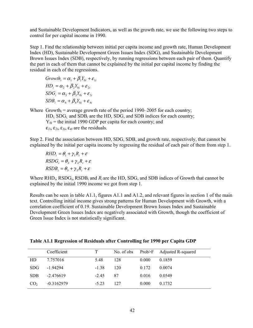
42
and Sustainable Development Indicators, as well as the growth rate, we use the following two steps to control for per capital income in 1990. Step 1. Find the relationship between initial per capita income and growth rate, Human Development Index (HD), Sustainable Development Green Issues Index (SDG), and Sustainable Development Brown Issues Index (SDB), respectively, by running regressions between each pair of them. Quantify the part in each of them that cannot be explained by the initial per capital income by finding the residual in each of the regressions.
iii YGrowth 1011 εβα ++=
iii YHD 2022 εβα ++=
iii YSDG 3033 εβα ++=
iii YSDB 4044 εβα ++=
Where Growthi = average growth rate of the period 1990–2005 for each country; HDi, SDGi, and SDBi are the HD, SDG, and SDB indices for each country; Y0i = the initial 1990 GDP per capita for each country; and ε1i, ε2i, ε3i, ε4i are the residuals.
Step 2. Find the association between HD, SDG, SDB, and growth rate, respectively, that cannot be explained by the initial per capita income by regressing the residual of each pair of them from step 1.
εγθ ++= ii RRHD 11 εγθ ++= ii RRSDG 22 εγθ ++= ii RRSDB 33
Where RHDi, RSDGi, RSDBi and Ri are the HD, SDG, and SDB indices of Growth that cannot be explained by the initial 1990 income we got from step 1. Results can be seen in table A1.1, figures A1.1 and A1.2, and relevant figures in section 1 of the main text. Controlling initial income gives strong patterns for Human Development with Growth, with a correlation coefficient of 0.19. Sustainable Development Brown Issues Index and Sustainable Development Green Issues Index are negatively associated with Growth, though the coefficient of Green Issue Index is not statistically significant. Table A1.1 Regression of Residuals after Controlling for 1990 per Capita GDP Coefficient T No. of obs Prob>F Adjusted R-squared
HD 7.757016 5.48 128 0.000 0.1859
SDG -1.94294 -1.38 120 0.172 0.0074
SDB -2.476619 -2.45 87 0.016 0.0549
CO2 -0.3162979 -5.23 127 0.000 0.1732
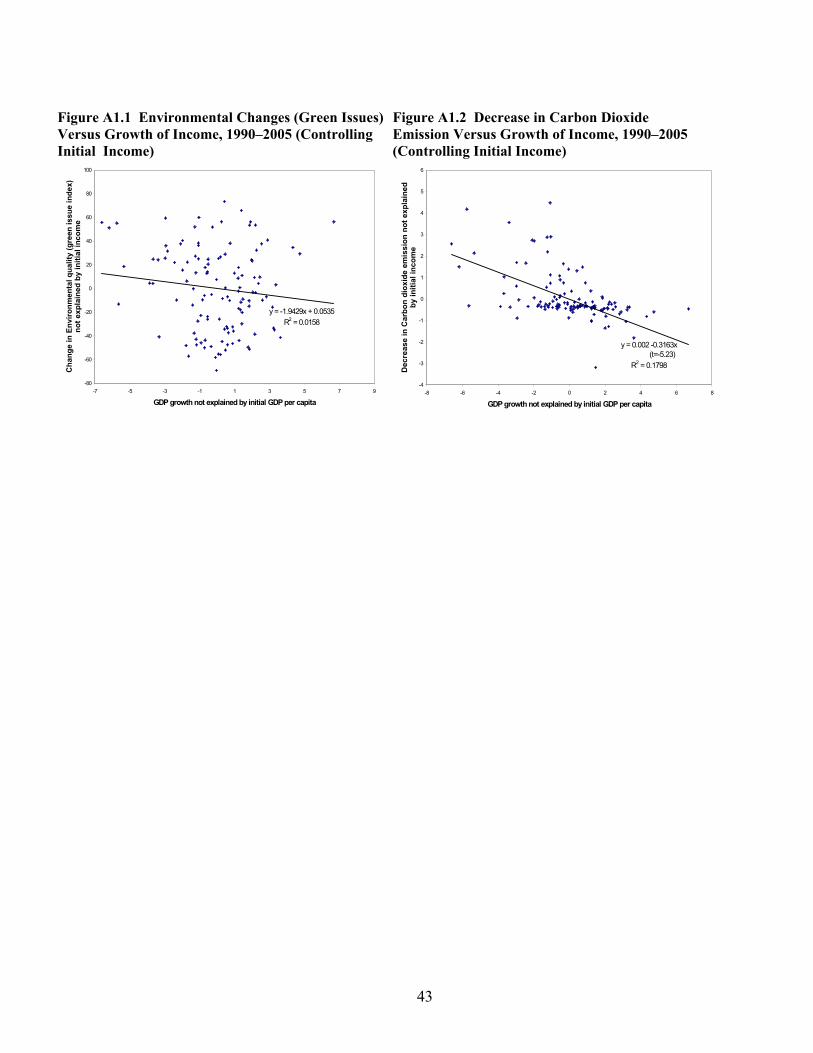
43
Figure A1.1 Environmental Changes (Green Issues) Versus Growth of Income, 1990–2005 (Controlling Initial Income)
y = -1.9429x + 0.0535R2 = 0.0158
-80
-60
-40
-20
0
20
40
60
80
100
-7 -5 -3 -1 1 3 5 7 9
GDP growth not explained by initial GDP per capita
Cha
nge
in E
nviro
nmen
tal q
ualit
y (g
reen
issu
e in
dex)
no
t exp
lain
ed b
y in
itial
inco
me
Figure A1.2 Decrease in Carbon Dioxide Emission Versus Growth of Income, 1990–2005 (Controlling Initial Income)
y = 0.002 -0.3163x (t=-5.23)
R2 = 0.1798
-4
-3
-2
-1
0
1
2
3
4
5
6
-8 -6 -4 -2 0 2 4 6 8
GDP growth not explained by initial GDP per capitaD
ecre
ase
in C
arbo
n di
oxid
e em
issi
on n
ot e
xpla
ined
by
initi
al in
com
e

44
Annex 2 A Conceptual Framework Conceptual Framework and the Central Hypotheses1
This note presents a rigorous—albeit nonmathematical—model showing how the interactions between certain market failures and government expenditure policies may condition economic development. (Readers interested in the underlying mathematical model, please refer to López 2007.) We emphasize certain important but generally ignored consequences of market failures for growth, efficiency, and social equity, showing how the orientation of government expenditures may exacerbate the negative impact of such market imperfections.
2.1 Market Failures We consider three types of market failure that potentially may cause the economy to underinvest in certain assets with the consequent losses in efficiency and growth capacity of the economy: (i) Asymmetric information and moral hazard in credit lending markets, which cause credit rationing and other capital market effects (Rothschild and Stiglitz 1976; Stiglitz and Weiss 1981). A subset of economic agents, mainly the lower-income ones, is not able to implement profitable investments because of borrowing constraints (Loury 1981). In addition, credit markets are affected by transaction costs, which cause a wedge between lending and borrowing rates. (ii) Externalities affecting mainly the environmental resources leading to excessive degradation of such resources (Dasgupta 1996) and spillovers in the generation, adoption, and diffusion of new knowledge, causing underinvestment in research and development and knowledge diffusion (Hoff and Stiglitz 2000). (iii) The well-known inability of a market economy to autonomously provide for conventional public goods or goods that tend to be nonexclusionary or nondepletable.
The obvious effect of (ii) is that the private economy tends to underinvest in environmental protection, research and development, and knowledge diffusion, while the effect of (iii) is underinvestment in conventional public goods. The effect of credit market failure on asset accumulation, equity, and growth is more complex and deserves a more detailed analysis.
2.2 Credit Market Failure and the Aggregate Levels of Investment in Physical and Human Capital2
We consider two types of credit market failure: credit rationing, caused by collateral requirements, and transaction costs, which cause a wedge between the costs of lending and borrowing money. Credit rationing affects only a portion of households and firms (presumably the least wealthy), while another portion is unconstrained; that is, they can borrow freely in the formal sector. To sharpen the analysis we assume that constrained firms and households cannot borrow at all in the formal credit market.
The fact that some firms can freely borrow at the market rate, while others cannot borrow in the formal market, confers an advantage to the former firms. The question is, why are the constrained firms still able to coexist with the unconstrained ones? Why are they not wiped out by the unconstrained firms? Constrained firms are able to subsist because, as a result of the existence of credit transaction costs, the 1 Prepared by Ramón E. López. 2 The mathematical model underlying this analysis can be found in López (2007a).

45
opportunity cost of their own capital (i.e., the rate at which they can obtain for their own liquid capital) is lower than the borrowing cost of credit in the formal market. This means that on a small scale of operations, based on owned capital only, the financially constrained firms can compete with firms that have access to commercial credit. The existence of these two types of credit market imperfections thus explains the often-observed coexistence of a sector of a few large firms with a great number of subsistence or semi-subsistence firms operating at a much-reduced scale of operations. This coexistence of large-scale firms with microenterprises is, of course, one of the most consistent stylized facts encountered, especially in poor and middle-income countries. To focus the analysis on the consequences of these types of credit market failure we need to make explicit some additional assumptions.
Assumptions
(1) The economy is small and open, firms and households are price takers in all markets (except the credit market, of course), and the unconstrained (large) firms can borrow freely in the international market; (2) firms produce a single output using physical capital and various types of labor skills (associated with the level of human capital and abilities of the workers) under constant returns to scale and a common production technology; (3) households use human capital combined with fixed factors (their level of ability and time resources) to produce labor power or productivity using a “production function” that, because of the existence of household fix factors, is subject to decreasing marginal product to human capital; (4) the various labor skills perfectly substitute for each other, up to a scale factor (that is, one hour of a high-skilled worker is equivalent to more than one hour of work by a lower-skilled worker).
Assumptions (1) to (3) are fairly standard in the literature. Assumption (4) is less conventional but is only made to reduce the dimension of the labor market effectively to just one market. This assumption allows for the existence of a composite wage rate and for the existence of a “labor power” aggregator.3 To derive the wage structure in the economy there is a need to determine only the composite wage rate. Once that basic wage rate is determined, all of the other wage rates for the remaining skills are proportional to the productivity differences. This is obviously quite an unrealistic assumption, but one needs to keep in mind that the focus of the analysis is not the labor market, and that relaxing this assumption is unlikely to change the results qualitatively.
The households’ and the economy’s total supply of human capital and skills
Credit market imperfections have particularly important consequences for the economy’s level of aggregate human capital investment. Households’ investments in human capital allow them to increase their skill levels and productivity, and thus attain a higher wage.4 Households affected by financial constraints may underinvest in human capital; that is, the marginal returns to human capital may remain above the (social) cost of human capital. Underinvestment in human capital by financially constrained households cannot be substituted with equal efficiency by more investments among (usually wealthier) households that are not financially constrained. This is the result of the fact that the marginal product of human capital, as a source of labor power, is decreasing because of the existence of fixed factors, including the household’s natural ability and time. This imperfect substitution among 3 The composite wage is equal to the weighted average of the wages corresponding to each skill level, and the labor power aggregate corresponds to the weighted sum of all labor using the skills as weights. 4 The wage structure is given to the households. See footnote 4 for details about the determination of the composite wage and the distribution of the wage structure in general equilibrium.

46
households’ investment in human capital means that if an important segment of the households is financially constrained, there is a net underinvestment in human capital and, consequently, undersupply of skills for the whole economy, as well as efficiency losses.
Physical capital accumulation and the firm sector
By contrast, the underinvestment in physical (and financial) capital by firms affected by financial constraints can be more easily compensated for by greater investments by firms that do not face financial constraints in the capital markets. In fact, given the assumption of constant returns to scale in assumption (2), investment substitution across firms may prevent any direct impact of the credit market imperfection on the aggregate level of investment in physical capital. It only causes changes in the distribution of investment across firms.5 There is, however, an indirect effect of the credit market failure on the investment in physical capital: The underinvestment in human capital causes the marginal product of physical capital to be lower and, hence, the incentives to invest in physical capital are also diminished.
Lobbying and the capturing of government expenditures
The credit market imperfections naturally induce governments to intervene by subsidizing firms or households. The availability of subsidies induces lobbying and other forms of rent seeking by interest groups to exert pressure upon the government to affect the allocation of subsidies in their favor. We argue that, for several reasons, the availability of subsidies to firms is more likely to elicit lobbying and rent seeking than the subsidies to households. First, the fact that the number of firms is fewer than the number of households implies that organizing producers is easier than organizing households. Second, firms are more easily grouped by production activities, with clear common interests, than households that tend to be much more dispersed both activity-wise and geographically. Third, the fact that most industries exhibit a high degree of concentration means that effective and powerful lobbies can be easily organized around a few dominant firms. Fourth, from the point of view of public acceptance, it is much easier to justify the existence of producers’ associations (even if controlled by a few large firms) influencing government for the sake of the productive sector that they represent than an association of a few wealthy households lobbying for a larger share of, for example, food stamps or public housing benefits.
5 There are three endogenous variables for the economy: the composite wage rate, the level of physical capital, and the level of total labor power (in turn dependent on the level and distribution of human capital across households). The composite wage rate is solved by the equality of the marginal return to capital of the financially unconstrained firms and the exogenous (international) cost of borrowing. Given Assumptions (1) and (2), the marginal return to capital of the unconstrained firms is a function only of exogenous output and input prices and the wage rate and independent of the level of physical capital. This equilibrium condition uniquely solves for the equilibrium composite wage rate. The other equilibrium condition is the equality of supply of and demand for total labor power. Given the composite wage-rate level, the demand for labor power is linear in the total stock of physical capital. In particular, given Assumption (2), the demand for labor power is independent of the distribution of capital across firms. The supply of labor power, on the other hand, depends on the level of investment in human capital that the households make. The supply of labor power does depend on the distribution of human capital across households; in particular, the larger is the proportion of financially constrained households and the lower is the total supply of labor power. The supply of labor power is solved at the household sector with constrained households’ investment in human capital determined by the availability of owned savings and unconstrained households setting human capital optimally.

47
This sharp contrast in lobbying potential between firms and households helps to explain an important stylized fact: Most firm subsidies are taken by very few firms, typically the wealthiest and most powerful ones, while most of the small firms receive very little of the subsidies. This is the case, despite the fact that the public justification for many such subsidies is to protect the small enterprises “affected by lack of credit.”6 For the reasons mentioned above, the availability of subsidies directed toward firms is likely to trigger much more lobbying and directly unproductive rent-seeking activities than the availability of subsidies directed toward the household sector. The much lower level of lobbying efforts elicited by subsidies to households imply that such subsidies tend to either concentrate on the lower-income households (some social transfers, food stamps, public housing) or, at worst, they more or less get evenly dispersed across households (free primary and secondary education, healthcare, social security, and others). The key issue is that the lower-income households (the most likely to face binding financial constraints) are able to get, at least, part of the cash or in-kind household subsidies, thus mitigating the effects of the financial constraints on their human capital investment, while the subsidies to firms tend to mainly create rents for the wealthier producers, which are the least likely to be affected by financial constraints.
Social equity and subsidies to firms and to households
Subsidies to firms and subsidies to households have dramatically different effects on social equity. We make the important distinction between structural inequality and other forms of inequality. Nonstructural inequality arising from a competitive system that allows for a level playing field is often considered to be necessary to generate adequate incentives for economic growth. Recent empirical evidence suggests, however, that inequality arising out of monopolized access to credit and natural resources, and the blatant exploitation of insider financial information, as well as nongovernmental policies that give especial privileges to certain politically and economically powerful groups, do not promote development.
From the previous section it is clear that government subsidies to firms tend to exacerbate structural inequality by transferring public resources mainly to the largest corporations, which are mainly owned by the wealthiest households. This negative equity effect of subsidies to firms is, of course, even worse if one considers that the raising of revenues in developing countries is based on a tax system that is both inefficient and inequitable. By contrast, subsidies to households, even if they are not targeted to the lower-income households, constitute a contribution to diminish structural inequality. To the extent that these subsidies are likely to become dispersed across poor, middle-income, and high-income household groups, they make a contribution toward easing the liquidity constraints on investments faced by the low-income and part of the middle-income households as a consequence of credit market failure. This, of course, contributes toward increasing opportunities for households that face constraints because of market imperfections; that is, to decrease structural inequality.
The following propositions summarize the implications of the above analysis:
Proposition 1. Government subsidies to households may help mitigate financial constraints that bind investments in human capital, thus increasing economic efficiency. Government subsidies to firms, however, do little to affect financial constraints on firms’ investments in physical capital. Also,
6 Farm subsidies are a good example of where a small minority of the largest farmers gets the lion’s share of them. The same is true for export subsidies, credit subsidies, and many other subsidies directed to firms.

48
subsidies to firms have a negative impact on economic efficiency by inducing more directly unproductive activities, while subsidies to households are less likely to do so.
Proposition 2. Subsidies to firms generally bypass the small enterprises often owned by poor households. Hence, the subsidies to firms generally fail to reach the poor households that own the small enterprises. That is, subsidies to firms contribute little to mitigating the effects of financial constraints affecting human capital investment by households.
Proposition 3. Government subsidies to firms are likely to promote more structural inequality while subsidies to households, even if not targeted toward the poor, help reduce structural inequality.
2.3 Taxonomy for Government Expenditures We consider two categories of government expenditures:
Type A are government expenditures that at least partly mitigate the effects of market failure, including environmental and knowledge externalities, credit market imperfections, and public goods incentives. Type A expenditures thus include government subsidies to households (including social expenditures, social transfers, education, and healthcare), environmental protection expenditures, research and development, and knowledge diffusion expenditures and expenditures in conventional public goods (law and order, infrastructure, culture, and others).7 These are mainly expenditures that tend to complement but do not substitute for the efforts of the private sector. For reasons explained in the following sections, we will broadly refer to all type A expenditures as expenditures in “public goods.”
Type B expenditures include subsidies directed toward firms, including credit subsidies, export subsidies, farm subsidies, financial bailouts, outright grants, and other forms of corporate welfare, often referred to as “development expenditures.” These are essentially government expenditures in private goods; that is, in goods that the private sector can optimally produce and therefore tend to be substituted with the latter. As shown by López and Galinato (2007) and others, type B expenditures often account for more than 50 percent of total government expenditures.
Social allocation of type A and type B expenditures
Earlier we argued that subsidies to households (including education, health, and other social transfers) generally do not elicit rent-seeking efforts in the private sector for their grabbing. The same is likely to be true for other type A expenditures as well. Public or semi-public goods, almost by definition, are hard to allocate to specific groups or individuals. This means that the lower-income groups, which are the ones most affected by credit market failures and other market imperfections, tend to share at least part of the benefits of type A expenditures.8
7 Pro-poor government expenditures and cash transfers to the poor are also considered Type A or public goods. These transfers contribute not only to increasing the consumption of the poor but also to reducing the financial constraints caused by credit market imperfections that constrain their investment in human capital. Ultimately they may thus have a positive effect on human capital accumulation and on economic growth. Similarly, government investments in protecting the natural environment have not only a direct welfare effect by improving quality of life but also a growth effect to the extent that a significant part of the natural environment (soils, water, and so forth) plays a role as a factor of production. 8 An exception is the lobbying from political representatives in parliament and other power centers that government expenditures in infrastructure elicit.

49
By contrast, type B expenditures are much more easily allocated to groups or even exclusively to particular individuals. Government credits and other financial subsidies, for example, are often captured by a small number of powerful and wealthy individuals that have the ability to effectively lobby and influence governments. The implication of this is that type B expenditures are much more lobby-driven than type A goods. Lobbying not only induces government to spend more on easily assignable expenditures (type B expenditures) but also to concentrate such expenditures in the often small and economically powerful groups and that are often the most effective lobbies. The implication of this is that, while the effects of type A expenditures tend to disperse among the population quite evenly, type B expenditures tend to end up appropriated by small elites, which are the least affected by market failure. Hence, type B expenditures tend to contribute little if anything to enhancing economic efficiency.
Moreover, the greater the availability of type B expenditures, the greater the incentives for the private sector to spend on directly unproductive activities, such as rent seeking, thus subtracting resources from economic growth. That is, type B expenditures, in addition to doing little to promote growth directly, stimulate greater waste by the private sector, which is unlikely to aid economic growth.
Government expenditures and the environment
The net effect of changing the structure of government expenditures on the environment is, in principle, ambiguous. The shift from type B to type A expenditures is likely to affect the environment in different directions: (a) output expansion effect has, ceteris paribus, a generally negative impact on the environment; (b) income expansion effect has a positive effect under the plausible assumption that environmental quality is a normal good; (c) output composition effect: the above expenditure shift is likely to have more powerful and direct effects on human capital than on physical capital. Also an important type A expenditure is knowledge generation and dissemination, which may benefit more knowledge-intensive industries. That is, this factor endowment effect is likely to increase the human-knowledge capital to physical capital ratio, thus altering the comparative advantages of the country in favor of human capital and knowledge-intensive activities, which are generally environmentally friendlier than physical capital-intensive activities. Therefore, the output composition effect is likely to be positive for the environment; (d) direct effects: A component of type A expenditures is environmental protection. Shifting expenditures toward type A may imply greater attention to environmental protection to mitigate the possibly negative implications of the output expansion effect for the environment. In addition, the type A expenditures include expenditures to perfect institutions, another important public good. To the extent that one of the biggest threats to the environment is the lack or imperfection of institutions to monitor and enforce environmental regulations, this effect is also likely positive.
Thus, while the net effect of switching the expenditure priorities of the government in favor of type A expenditures is in principle negative, most of the partial effects point in the positive direction. Only the output expansion effect may have a negative impact. Elucidating the effects of a government expenditure restructuring is an empirical issue, but a priori one may argue that the strength of the other offsetting effects is likely to be important. The direct effects (d), in this respect, is likely to be very decisive, because if powerful enough it could largely cancel out the only negative effect, the output expansion one.
The most important conclusion from the previous analysis is that the effect of transferring one dollar from type B to type A expenditures is likely to have important consequences:

50
2.4 Central Hypotheses
An exogenous reallocation of government expenditures from private to public goods, if it can be sustained over time, promotes: (i) faster economic growth, (ii) less structural inequality, (iii) a generally ambiguous effect on the environment, but several presumably powerful effects point in the direction of improving the environment. In particular, the direct effects (d) play the role of weakening the impact of the only other effect that is negative for the environment, the output expansion effect (a).
These hypotheses will be tested in the following three papers; summarized in annex 3.1, 4, and 5, respectively; and in addition, annex 3.2 presents supporting evidence from the project analysis.

51
Annex 3.1 Fiscal Policy and Economic Growth Summary of “The Structure of Public Expenditure: A Robust Predictor of Economic Development?” Background Paper 1 9 Introduction and Typology of Fiscal Expenditures This annex is based on López and Miller 2007 (background paper 1) exploring the impact of fiscal policy on economic growth, using data from a sample of 29 middle-income countries. The findings show that government provision of public goods and services is a key source of economic growth and that switching government expenditures from (nonsocial) subsidies to public goods is likely to have a dramatic effect in accelerating economic growth. Two categories of government fiscal expenditures are considered in the analysis. Type A (broadly defined as public goods): Those government expenditures that at least in part mitigate the effects of market failure on aggregate growth. That is, investment in goods that complement but not substitute for the efforts of the private sector in enhancing knowledge and human, natural, and physical capital; as well as goods that qualify as “pure” public goods. Type B. Government expenditures on private goods—goods that the private sector can optimally produce, or expenditures that do little to enhance the level of aggregate investment (see the conceptual framework in Annex 2). These are called expenditures in nonsocial subsidies. Model and Data The hypothesis is tested that an exogenous reallocation of government expenditures from private to public goods, if it can be sustained over time, promotes faster economic growth. Clearly the direction of causality between economic growth and fiscal policy (or more specifically the share of public goods expenditures in total government expenditures) is likely to be bidirectional rather than one way. That is, not only the share of public goods expenditures may affect growth but it is equally plausible that economic growth has an impact on how governments allocate their expenditures. A multi-equation system approach is used to deal with the simultaneous interdependencies among these two key variables. This allows for the above fiscal policy to be endogenously affected not only by economic growth but also by several control variables to be incorporated into the analysis, and allows for measuring the long-term growth effects of the fiscal policy. The benchmark model consists of a simultaneous system of two equations, as follows:
itpit
itp
it
itpit
it
kk
sy
Msy
ελ +⎟⎟⎠
⎞⎜⎜⎝
⎛⋅+⎟⎟
⎠
⎞⎜⎜⎝
⎛=⎟⎟
⎠
⎞⎜⎜⎝
⎛ ˆˆ
9 Based on a background paper by Ramón E. López and Sebastian Miller.

52
Where: • ity is per capita GDP growth in time t • p
its is the share of government expenditures in public goods • M is 2x2 matrix with a zero diagonal • itk
r is a vector of N control variables and instruments
• λ is a Nx2 matrix for the control variables • itε is a vector of disturbances
The two key endogenous variables are the rate of GDP growth and the share of expenditures on public goods in total government expenditures. Control variables include macroeconomic and fiscal variables and institutional-political variables, as well as country characteristics. Among the macro-fiscal control variables used are government consumption expenditures over GDP, taxes over GDP, and total investment (in physical and financial capital) over GDP.10 Other control variables used include per capita GDP at the beginning of the sample period (which accounts for the conditional convergence so often documented in the literature), inflation, schooling, and certain geographic variables as well as several political and institutional variables. Because of the large degree of instability of the annual GDP growth rate data (see the following paragraphs for more details about this), the econometric estimation uses averages over five years as the basic unit of observation as a way of smoothing the nonsystematic fluctuations. The benchmark analysis estimates the model using a sample restricted mainly to 29 middle-income countries for the period 1980–2004. The main sample of middle-income countries include 10 countries from Latin America, six countries of East Asia, four countries of South Asia, three European countries that at the beginning of the period (1980) were considered middle income but today are developed, and six countries mostly from the Middle East and Northern Africa (with the exception of Mauritius). A reason why the main sample focuses on mostly middle-income countries is that the key government expenditure and tax revenue data for poor countries is highly incomplete and in some cases of dubious quality. The main sample has not incorporated more developed countries in order to preserve a sample that may be considered representative of middle-income countries as of the early 1980s11 The main data for government expenditures are obtained from the Government Financial Statistics database compiled by the International Monetary Fund (IMF 2006). For some countries data provided by the Asian Development Bank (ADB 2006) are used. Expenditure data are provided by categories of expenditures according to the COFOG (classification of functional government expenditure) typology. A description of the data and their sources as well as definitions of variables is provided in Table A3.1.1.
10 The use of taxes over GDP in addition to total government consumption expenditure is not a problem in the model since the sample of developing countries has a relatively low correlation between taxes and government consumption. 11 The following criteria to define the country sample are used in the benchmark regressions: Countries that were considered middle income in the 1980s and have enough data for at least three observations when using five-year averages over the period 1980–2004. This yields the benchmark data sample of 29 countries.

53
Empirical Results The benchmark results estimated using the three-stage least square approach are presented in Table A3.1.2. The key finding is the positive and significant effect of the share of expenditures on public goods on growth of per capita GDP. Economic growth also shows a positive and significant effect on the share of expenditures in public goods. Despite, however, that the values of the point estimates of the coefficients may suggest otherwise, the latter effect is smaller than the effect of share of public goods on growth in relative terms. In fact, the elasticities evaluated at mean values are 2.22 for the effect of public goods on growth, while the elasticity of growth on the share of public goods is only 0.13 (both are significant at 1 percent though). Therefore, changes in the share of public goods have a much more significant effect on growth than vice versa. Aggregate government consumption has a negative but nonsignificant effect on growth. This result, unlike the findings concerning the share of public goods, is not robust. In general, when controlling for taxes over GDP the effect of government expenditures tends to become positive but not necessarily significant (and taxes negative and significant in some cases) while otherwise the effect tends to be negative. These results are consistent with the inherent ambiguity of the effect of government total consumption on per capita growth. The effect crucially depends on how governments finance these expenditures. Since countries in the sample are likely to use very different mechanisms of financing government expenditures the estimated effects are almost by definition weak. The effect of total investment over GDP is fully consistent with the findings of previous studies; it exerts a positive and significant effect on economic growth. Another result that is consistent with the vast majority of previous studies is the prevalence of conditional convergence. A lower initial level of per capita GDP predicts higher growth rates. As can be seen in Table A3.1.2 the coefficient of the initial per capita GDP is negative and statistically significant. There is potential for endogeneity in some of the variables, especially in taxes, government consumption, and the level of investment. When controlling for government consumption over GDP as an endogenous variable in a three-equation system, however, the result is the same about the effect of the share of public goods expenditures on growth. Similarly, when using predicted values (via instruments) for government consumption over GDP, taxes over GDP, and investment over GDP in the two-equation system or instrumenting the latter two variables in the three-equation system, the share of expenditures in public goods is still positive and statistically significant. Finally and mainly for the sake of comparison with the previous literature, single-equation estimations using instrumental variable (IV) (two-stage least squares, 2SLS), weighted least squares and random effects methods are performed. The results confirm that the share of expenditures on public goods is positive and statistically significant for per capita GDP growth. Based on calculations using the results from Table A3.1.2, the net effect from an “exogenous” policy that might affect the share of expenditures on public goods is 3.14, the long-run elasticity that includes both the feedback effects as well as the direct effects of a raise in the share of public goods. The first-round increase in the growth rate leads to a second-round expansion of the share of public goods, thus further enhancing the effect on growth.

54
Sensitivity Analysis A series of sensitivity analysis on the benchmark results reported in Table A3.1.2 is conducted. Specification checks show that when treating taxes over GDP as an additional endogenous variable thus estimating a four-equation system, or using a five-equation system assuming all five variables (economic growth, government consumption over GDP, share of public goods in total public expenditures, taxes over GDP, and investment over GDP) are jointly determined, the key results remains unaltered: the share of public goods expenditures has a positive and significant effect on growth. A check on control variables dominance and omitted variables shows that adding new control variables to and taking controls out of the equations, the estimates for the share of public goods expenditures remain positive and significant (see figure A3.1.1). A sample dominance check demonstrates that when excluding observations corresponding to the top 10 percent and bottom 10 percent of the values of the share of public goods expenditures alternatively, dropping the top and bottom 5 percent of observations simultaneously, or conducting a bootstrap resampling, estimates for the effect of the share of public goods remain positive and significant. A related country dominance check shows that dropping one country at a time from the original system, the point estimate is always positive and the 95 percent interval of the coefficient is always within the positive range regardless of which country is removed from the sample. In other words, there is no single dominant country that forces the results. Also, when adding 18 developed countries and some additional middle-income countries to the sample to form a new data set comprising 58 countries, the results basically tell the same story: there is a positive and statistically significant effect of the share of public goods on growth, though the coefficient is now smaller in size and the level of significance is lower.

55
Table A3.1.1 Description of Variables and Data Used in the Analysis
Variable Description Years Available
Source
GDP per Capita Real GDP per capita (constant USD2000) 1980–2004 World Development Indicators (World Bank)
Share of Govt. Exp. in Public Goods
This is the share of government expenditure on public goods. Public goods are defined as a total of: i) Education ii) Health iii) Social security iv) Transport v) Communication vi) Public order and safety vii) Housing and community amenities
1980–2004 Government Financial Statistics (IMF), Asian Development Bank, country data
Share of Investment over GDP
1980–2004 Penn World Tables (2006)
Years of Schooling Average years of schooling of population over 15 1980–2000 (5-year interval)
Barro and Lee (2001)
Share of Govt. Exp. over GDP
1980 –2004 Penn World Tables (2006)
Ecological Footprint of Production
This is the biological capacity needed to produce the goods and services consumed and assimilate waste by the people in a country, without any imports and exports. This is a measure for the domestic resource demand. The components are i) crop production, ii) animal production, iii) fish production, iv) forest products, v) built-up land, and vi) fossil energy
1961– 2003 Global Footprint Network, http://www.footprintnetwork.org/
Years of Democratic Stability
Square root of Durability of Polity if Polity 2>0 1980–2005 From Polity IV and updated to 2005
Dummy Freedom of Press 1 if print media is considered free 1980–2005 www.freedomhouse.org Polity Index (Polity 2)
Score that indicates how democratic a country is 1980–2003 Polity IV www.cidm.umd.edu
Political Competition Score that indicates how competitive the political system is
1980–2003 Polity IV www.cidm.umd.edu
Initial Income Gini 1980 or earliest available Gini used N/A World Income Inequality Database % Land in Tropical Areas Fraction of land area in tropics N/A Gallup, Sachs, and Mellinger
(1999) Dummy Landlocked Dummy variable taking value of 1 if country is
landlocked, 0 otherwise. N/A Dollar and Kraay 2002
Corruption Perception Index
Average score of CPI 2000–5 NA Transparency International www.transparency.org
Education Gini Measuring education inequality: Gini coefficients of education for 140 countries
1960–2000 Thomas, Vinod, Yan Wang, Xibo Fan, 2003, p. 5–33.
Trade Openness Sati Index, which is the residual of the regression of Trade on population, area, GDP per capita, dummy for industrialized country, dummy for oil exporter, and imports over export prices. A positive residual implies a more open economy.
1980–2001 Pritchett, Lant. 1996. Updated by López and Galinato (2007)
Ethnolinguistic Fractionalization 1961
Score of Ethnolinguistic Fractionalization in 1961 N/A Philip G. Roeder, 2001.”Ethnolinguistic Fractionalization (ELF) Indices, 1961 and 1985.”

56
N/A = not applicable
<http//:weber.ucsd.edu\~proeder\elf.htm>.
Share of Primary Commodity Exports
Primary commodity exports include food, agricultural raw materials, fuels, ores, and metals
1980–2004 United Nations Commodity Trade Statistics Database (UN COMTRADE)
Share of Indirect Taxes Share of Indirect Taxes over Total Revenue 1980–2004 Government Financial Statistics (IMF)
Federal Country Dummy 1 if country is Federal N/A Handbook of Federal Countries: 2002, Montreal and Kingston: McGill-Queen’s University Press, 2002.
Malaria Ecology Malaria Ecology is an ecologically based spatial index of the stability of malaria transmission based on the interaction of climate with the dominant properties of anopheline vectors of malaria that determine vectorial capacity (Kiszewski et al., 2004). The Malaria Ecology variable measures the effects of ambient temperature on the force of transmission of malaria, as expressed through the length of the extrinsic incubation period, and therefore the proportion of the vector population able to survive long enough to become infectious.
N/A Sachs et al. (2004)
Distance to the Equator Distance from Equator, measured as absolute value of latitude of capital city.
N/A Dollar and Kraay 2003
Presidential Dummy 1 if system is considered presidential in nature (0 or 1 in Database of Political Institutions)
1980–2003 Database of Political Institutions, Beck, Thorsten, et al.

57
Table A3.1.2 Three-Stage Least Squares System of Equations: Benchmark Estimation
Growth of GDP per Capita
Share of Govt. Exp. in Public Goods in Total Govt. Expenditure
2.963** Growth of GDP per Capita [1.318] 0.098*** Share of Govt. Exp. in Public
Goods in Total Govt. Expenditure [0.033] -0.007 -0.139 Total Govt. Consumption over
GDP [0.026] [0.137] -0.078** 0.429** Taxes over GDP
[0.036] [0.205] 0.074** -0.390* Total Investment over GDP
[0.037] [0.204] -0.008*** Log of Initial per Capita GDP [0.003] -0.001* 0.003 Inflation (CPI) [0.001] [0.004] 0.009 0.002 Lag of Log Years of Schooling [0.007] [0.030] 0.002** -0.002 Years of Democratic Stability [0.001] [0.005] -0.281*** Corruption [0.073] -0.012** % Land in Tropical Areas [0.005] 0.064* Malaria Ecological Index [0.036] -0.019** 0.218*** Dummy Latin America [0.008] [0.029] 0.003 0.006 Dummy Developed Countries [0.008] [0.044] 0.014* -0.073* Dummy East Asia [0.008] [0.043] 0.037* 0.605*** Constant [0.019] [0.102]
Small sample standard errors in brackets; estimates include year dummies not shown in table; no. of countries: 29; obs. = 105. * significant at 10%; ** significant at 5%; *** significant at 1%

58
Table A3.1.3 Single Equation Estimates of per Capita GDP Growth
IVa IV-WLSb RE 0.102*** 0.099*** 0.035** Share of Govt. Exp. in Public Goods
in Total Govt. Expenditure [0.026] [0.026] [0.017] -0.012 -0.007 -0.023 Total Govt. Consumption over GDP [0.028] [0.028] [0.026] -0.072*** -0.072*** -0.05 Taxes over GDP
[0.028] [0.027] [0.035] 0.088** 0.086** 0.091** Total Investment over GDP
[0.035] [0.036] [0.038] Initial GDP per Capita -0.010*** -0.010*** -0.009*** [0.003] [0.003] [0.003] Inflation (CPI) -0.001 -0.001 -0.001* [0.001] [0.001] [0.001] Lag of Log Years of Schooling 0.012** 0.012* 0.012* [0.006] [0.006] [0.007] Years of Democratic Stability 0.001 0.001 0.002** [0.001] [0.001] [0.001] % of Land in Tropics -0.007 -0.007 -0.011* [0.006] [0.006] [0.006] Dummy Latin America -0.019*** -0.018*** -0.006 [0.007] [0.007] [0.007] Dummy Developed Countries 0.007 0.007 0.006 [0.008] [0.008] [0.009] Dummy East Asia 0.01 0.011 0.009 [0.008] [0.008] [0.008] Constant 0.021 0.039*** 0.044** [0.016] [0.015] [0.018] Observations 105 105 P-Value of Hausman Test of Consistency of RE Estimates
0.7629
Robust standard errors in brackets (except FE and RE); Estimates include year dummies not shown in table; * significant at 10%; ** significant at 5%; *** significant at 1% a Instrumented variable: Share of Govt. Exp. In Public Goods; Excluded Instruments: Malaria Ecological Index, Corruption. b Weighted Least Squares by log of population.
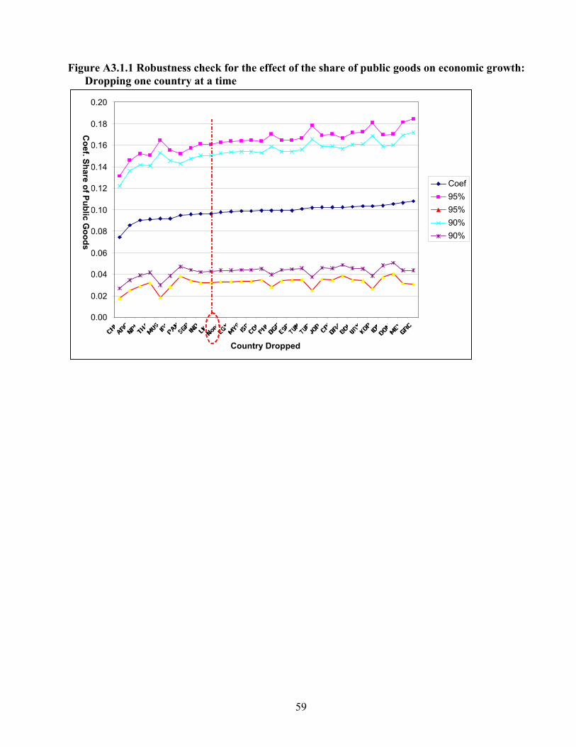
59
Figure A3.1.1 Robustness check for the effect of the share of public goods on economic growth: Dropping one country at a time
0.00
0.02
0.04
0.06
0.08
0.10
0.12
0.14
0.16
0.18
0.20
Country Dropped
Coef95%95%90%90%
Coef. Share of Public G
oods

60
Annex 3.2 Project Analysis: Composition of Public Expenditure Key to Project Success12 Introduction The project-level analysis investigates the correlation between the performance of World Bank loans and the fiscal policy environment of borrowing countries, focusing on the link between project performance and government spending on public goods. Government resource-allocation decisions affect project outcomes by influencing the macroeconomic environment throughout the project life cycle. Governments allocate scare resources between investments in public goods and subsidies. By assumption, subsidies do not contribute productively to projects financed by the World Bank; therefore, a government's decision to prioritize subsidies at the expense of public goods will, other things equal, reduce the probability of a project meeting its objectives by reducing productive resources allocated to public projects. Allotting a greater share of revenue to subsidies reduces the government's capacity to implement and operate projects by diverting resources away from World Bank projects. Human capital is diverted when government employees are taken away from project oversight to the management of subsidies (often a complex undertaking). Subsidies are substitutes for the financial resources needed for project operation. A government that chooses not to invest in its people reduces the overall level of human capital available, creating a relatively low-skilled labor force. Government spending on public goods should, other things equal, increase the stock of human capital in a country by increasing resources allocated to providing health care and education. The poor suffer disproportionately from a lack of government-provided health and education as they lack the financial means (including access to credit) to substitute private services for public services. The poor may also underinvest in health and education, if, as seems likely, their discount rate is higher. Government spending on social public goods to correct market failures is assumed to increase the productivity of public investment projects. Government spending on nonsocial public goods, such as basic infrastructure, ensures the necessary physical assets for project implementation, operation, and utilization. Previous research linking micro-level loan data to macroeconomic variables suggests the economic environment in which projects are undertaken is crucial to project success. Macroeconomic stability, trade openness, the black-market premium on a countries foreign exchange, and the quality of institutions played important roles. Model and Data The data used in this analysis are overall project outcome ratings provided by the Independent Evaluation Group (IEG) of the World Bank. IEG evaluates all completed World Bank projects—approximately 300 projects per year. Evaluations are typically conducted one to two years after a project has closed. A project is closed when all funds have been disbursed. The duration of World Bank projects varies; for the period covering 1980–2005 the average project length was six years. Projects are generally operational at the point of final disbursement. IEG evaluations are, therefore, generally conducted after a project has been operational. The majority of evaluations consist of reviews of Implementation Completion Reports provided by operational units. In the estimation sample, 67 percent of the evaluation data are based on Implementation Completion Report reviews, while the remaining 33 percent are based on more in-depth audits performed (including visits to the field by IEG evaluators). Project outcomes vary between countries because of differing policy environments and other country characteristics. They also vary within countries and over time because of changes in policies and economy-wide shocks. The major 12 Based on a background note prepared by Ann Flanagan.

61
source of variation in our data set is cross-sectional.13 The satisfactory rates of World Bank projects at the country level range from 30 percent (Vanuatu and the Democratic Republic of Congo) to 100 percent (Czech Republic and Latvia). There were 2,477 projects approved and evaluated between 1980 and 2005 in these countries with an average of 95 projects per year and 29 projects per country. Overall project outcome ratings are determined based on an assessment of the relevance of the interventions' objectives relative to country priorities and needs, the extent to which the stated development objectives are achieved, and cost-effectiveness. The productivity of World Bank investments is captured through IEG's outcome rating: countrywide policies, including government public spending programs, are likely to influence both the choice of output and the capacity utilization of projects once completed (Isham and Kaufmann 1999). Given the nature of IEG’s rating data, we model the probability of project success (as defined by a satisfactory IEG rating) assuming a logistic distribution for the error term. We estimate three regression models. First, we estimate a model to test whether or not the share government spending allocated to public goods has an impact on the overall project outcome rating of World Bank projects. We assume a continuous, unobserved latent variable that is related to IEG’s outcome rating by the following structural equation: (1) y*
ijt = xijtβ + εijt where 1=yijt if y*ijt >0 and 0=yijt if y*ijt ≤ 0 and the x denotes project-specific variables such that:
(2) ∑
∑
i
i j
n
1=tijt
ijtn
∑∑x=x
where i represents projects, j represents the country in which the loan was conducted, and t is the year of loan approval. Variables measured at the country level are constructed as project-specific variables by taking the average values over project duration, therefore, t=1,2,…n defines the duration of the project from approval to exit fiscal year. Ordered logistic regressions were used estimate the relationship between IEG project outcome ratings and the share of government spending on public goods. An ordinal regression model can be expressed as latent variable model where y* is the continuous latent variable. The observed ordered responses are linked to the latent variable through a measurement equation of the form:14 (3) yijt = m if τm-1 ≤ y*
ijt < τm for m = 1,2,…6 and the cut points τ0,τ1,τ2,τ3,τ4, and τ5 are estimated and the latent variable y*
ijkt crosses a cut point at observed category changes. Given the change in project rating scheme in the mid-1990s, the logistic estimation approach was used to estimate the equation for the entire period (1980–2005) and an ordered logistic approach was employed
13 With large N relative to t and primarily cross-sectional variation in the variables of interest, fixed effects regression is inappropriate. 14 Long, J. Scott and Jeremy Freese 2006. Regression Models for Categorical Dependent Variables Using Stata (2nd Edition). College Station, TX: Stata Press.
62
after the change (1994–2005) period to utilize the greater variation in project outcome ratings. Differences in country policies are likely to influence the success of public investment projects. Country-level macroeconomic variables are used to control for differences in the policy environments across countries and over time. Table A3.2.2 presents a set of summary statistics of variables used in the project-level analysis (see Table A3.1.1 for definitions). Statistical Results Table A3.2.3 presents simple correlations between IEG project outcome ratings, our main variable of interest—the share of public spending on public goods—and project-level characteristics and country-level characteristics that are hypothesized to influence project success. Among the macroeconomic variables, theory and previous research limited the inclusion of relevant variables. For example, Isham, Kaufmann, and Pritchett (1997) found countries with better institutions have higher rates of return, other things equal, and the magnitude of the impact of institutions on government efficacy is greater than the influence on economic distortions. As Isham and Kaufman (1999) note, the black market premium is a relatively comprehensive indicator of trade distortions at the country level. Trade openness is assumed to capture the possible productivity increases associated with the flow of information and technology that is likely to affect project outcomes. Past research testing the role of aid has found absorptive capacity constrains aid’s effectiveness (Dollar and Levin 2005 and Guillaumont and Lajaaj 2007). The main estimation results are presented in Table A3.2.3. The relationships between the probability of a satisfactory outcome rating and the share of public spending on public goods and the set of project and country-level characteristics for the entire period (1980–2004) are given in columns 1 and 2; the relationships between these variables and the probability of each outcome rating for the 1994–2004 period are given in columns 3 and 4. Primary interest lies in whether or not the share of public spending on public goods is correlated with the overall success of World Bank projects. In the growth-aid debate, evidence using IEG project-level data suggests that aid effectiveness is highly dependent on country-level institutional environment. Sound institutions are likely to both emphasize public spending and growth. The key finding is the positive and significant correlation between the share of spending on public goods and project success. The share of spending on public social goods is positively and significantly related to World Bank project success. For projects evaluated between 1994 and 2005, a one standard deviation increase in the share of spending allocated to public goods (approximately 20 percentage points) is associated with a 5 percentage point increase the net probability of project success for the average country. Sensitivity Analysis There is possibility of reverse causation in that good institutions—in this case measured by the lack of corruption—likely increase the probability of project success and project success may reinforce strong institutions. As well, as in the case of aid, the possibility of negative spurious correlation exists when countries experiencing negative shocks also have lower project outcome ratings. To test for these endogeneities, an instrumental variable regression approach was employed following the methodology of Dollar and Levin (2005). Table A3.2.5 presents these results.

63
The key result remains. The share of spending on public goods is positively and significantly associated with the percent of satisfactory projects at the country level, and public spending dominates institutions. Table A3.2.1 Variable Definitions Variable Definition Complex Project Indicator IEG evaluation database. Share of Government Spending on Public Goods in Total Government Spending
This is the share of government expenditure on public goods. Public goods are defined as a total of education, health, social security, transport, communication, public order and safety, and housing and community amenities taken from the Government Financial Statistics (IMF).
Share of Government Spending on Social Public Goods in Total Government Spending
This is the share of government expenditure on social public goods. Social public goods are defined as a total of education, health, and social security, taken from the Government Financial Statistics (IMF).
Share of Government Spending on Nonsocial Public Goods in Total Government Spending
This is the share of government expenditure on nonsocial public goods, defined as public goods minus those social public goods.
Share of Government Spending in GDP
Total Government spending as a percent of real GDP (Penn World Tables).
Capital-Labor Ratio (World Development Indicators) Terms of Trade Exports at current prices divided by exports at constant prices relative to
imports at current prices divided by imports at constant prices (World Development Indicators)
Government Surplus (% GDP) Government Financial Statistics Black Market Premium Ration of the black market exchange rate and official exchange rate minus
one. Trade Openness Sati index, which is the residual of the regression of Trade on population,
area, GDP per capita, dummy for industrialized country, dummy for oil exporter, and imports over export prices. A positive residual implies a more open economy (Pritchett, Lant 1996. Updated by López and Galinato (2007).
Inflation (% annual) World Development Indicators GDP per Capita Growth Rate World Development Indicators Composite Risk Rating, ICRG An index assessing political, economic, and financial risk at the country
level (ICRG). Composite Political Risk Rating, ICRG
An index assessing the degree of government stability, socioeconomic conditions, investment profile, internal conflict, external conflict, corruption, military in politics, religious tensions, law and order, ethnic tensions, democratic accountability, and bureaucratic quality in a country (ICRG).
Corruption Index, ICRG An assessment of the degree of corruption in the political system. Corruption distorts the economic and financial environment, and reduces government efficiency by enabling nepotism, patronage, and economic instability (ICRG).
Law and Order Index, ICRG An assessment of the strength and impartiality of the legal and judicial system and popular observance of the law (ICRG).

64
Table A3.2.2 Summary Statistics: 1980–2004 Variable Obs Mean Std. Dev Min Max Share of Gov’t Spending, Nonsocial Public Goods 2,478 0.09 0.048 0.000 0.267 Share of Gov’t Spending, Public Goods 2,478 0.42 0.182 0.027 0.832 Share of Gov’t Spending, Social Public Goods 2,477 0.33 0.164 0.026 0.756 Annual GDP per Capita Growth Rate 4,750 2.00 3.48 -15.92 43.08 Official Development Aid 4,713 7.07 10.16 -0.072 125.34 ICRG Index 3,780 59.82 10.15 22 82.01 CPIA Index 3,682 3.35 0.581 1 5.4 Years of Education, Population 15+ 3,366 4.72 2.146 0.49 10.84 Quality-Adjusted Years of Education, Population 15+
2,745 2.74 1.676 0.116 7.298
Life Expectancy at Birth 4,701 61.02 9.954 27.42 78.01 Terms of Trade Improvements 4,345 -0.46 3.924 -23.76 56.82 Capital-Labor Ratio 4,209 1.07 0.158 0.436 2.525 Government Deficit % GDP 4,144 -8.95 93.71 -1911 13.91 Black Market Premium 4,277 437.26 4827 -8.01 102623 Trade Openness 3,745 -4.142 27.12 -63 165.75 Real Interest Rate 3,931 8.23 14.60 -98.15 97.94
Table A3.2.3 Correlation between IEG Overall Project Outcome Ratings and Key Project Variables
Variables Overall Project Outcome Rating
Complex Project Indicator -0.0920*** Share of Government Spending on Public Goods in Total Government Spending 0.1495*** Share of Government Spending on Social Public Goods in Total Government Spending 0.1476*** Share of Government Spending on Nonsocial Public Goods in Total Government Spending 0.0519** Share of Government Spending in GDP -0.0013 Capital-Labor Ratio 0.1583*** Terms of Trade -0.0219 Government Surplus (% GDP) 0.061 Black Market Premium -0.1137* Trade Openness 0.0089 Inflation (% annual) -0.1182* GDP per Capita Growth Rate 0.2705*** Composite Risk Rating, ICRG 0.2611*** Composite Political Risk Rating, ICRG 0.2119*** Corruption Index, ICRG 0.1176*** Law and Order Index, ICRG 0.1569***
Note: *** indicates significance at the 1 percent level, ** significance at the 5 percent level, and * significance at the 10 percent level.

65
Table A3.2.4 Logistic and Ordered Logistic Estimation Results, Dependent Variable IEG Project Outcome Rating 1980-2005 1980-2005 1994-2005 1994-2005 Logit Logit Ordered
Logit Ordered Logit
Probability of project being rated as satisfactory Pr(Sat) Pr(Sat) Pr(Out) Pr(Out) AFR 0.133 0.189 0.141 0.141 [0.573] [0.436] [0.560] [0.567] EAP 0.132 0.298 0.268 0.343 [0.548] [0.188] [0.175] [0.089]* ECA -0.327 -0.288 -0.16 -0.39 [0.151] [0.243] [0.427] [0.081]* LCR -0.321 -0.478 0.083 -0.203 [0.124] [0.032]** [0.670] [0.335] SAR 0.044 0.548 0.002 0.144 [0.851] [0.066]* [0.994] [0.615] Dummy Complex Project = 1 0 = Otherwise 0.068 0.024 0.115 0.084 [0.816] [0.934] [0.619] [0.719] Dummy PPAR = 1 0 = Otherwise -0.144 -0.119 0.009 0.025 [0.215] [0.308] [0.937] [0.827] Dummy Investment Loan = 1 0 = Otherwise -0.149 -0.124 -0.528 -0.524 [0.548] [0.621] [0.016]** [0.017]** Initial GDP (Logs) 0.219 0.177 0.239 0.27 [0.020]** [0.081]* [0.006]*** [0.004]*** Corruption Index, ICRG 0.192 0.103 0.203 0.131 [0.003]*** [0.125] [0.002]*** [0.058]* GDP per Capita Growth Rate 0.224 0.201 0.218 0.195 [0.000]*** [0.000]*** [0.000]*** [0.000]*** Share of Spending on Public Goods in Total Gov’t Spending
2.182 1.364
[0.000]*** [0.003]*** Share of Government Spending in GDP 0.813 2.275 [0.409] [0.019]** Constant -0.597 -1.113 [0.442] [0.193] Observations 2165 2161 1568 1564 Absolute value of z-statistics in brackets * significant at 10%; ** significant at 5%; *** significant at 1% Note: Estimated equations include annual time dummies and sector dummies.
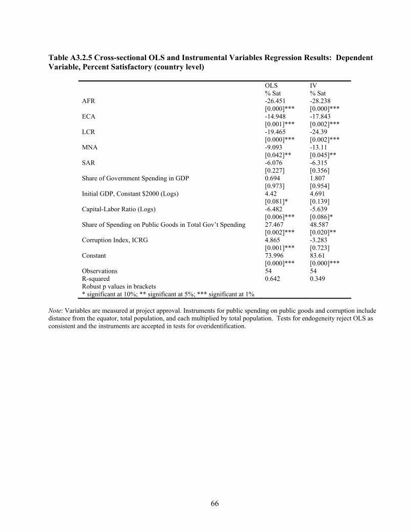
66
Table A3.2.5 Cross-sectional OLS and Instrumental Variables Regression Results: Dependent Variable, Percent Satisfactory (country level)
OLS IV % Sat % Sat AFR -26.451 -28.238 [0.000]*** [0.000]*** ECA -14.948 -17.843 [0.001]*** [0.002]*** LCR -19.465 -24.39 [0.000]*** [0.002]*** MNA -9.093 -13.11 [0.042]** [0.045]** SAR -6.076 -6.315 [0.227] [0.356] Share of Government Spending in GDP 0.694 1.807 [0.973] [0.954] Initial GDP, Constant $2000 (Logs) 4.42 4.691 [0.081]* [0.139] Capital-Labor Ratio (Logs) -6.482 -5.639 [0.006]*** [0.086]* Share of Spending on Public Goods in Total Gov’t Spending 27.467 48.587 [0.002]*** [0.020]** Corruption Index, ICRG 4.865 -3.283 [0.001]*** [0.723] Constant 73.996 83.61 [0.000]*** [0.000]*** Observations 54 54 R-squared 0.642 0.349 Robust p values in brackets * significant at 10%; ** significant at 5%; *** significant at 1%
Note: Variables are measured at project approval. Instruments for public spending on public goods and corruption include distance from the equator, total population, and each multiplied by total population. Tests for endogeneity reject OLS as consistent and the instruments are accepted in tests for overidentification.
67
Annex 4 Fiscal Policy, Growth, and Income Distribution Summary of Background Paper 2 15 Introduction This annex is based on López and Torero 2007 (background paper 2) exploring the impact of fiscal policy and economic growth on income distribution, using household survey data available for several years in a sample of 37 developing countries over the 1985–2004 period. Two broad issues are examined: First, how the benefits of economic growth spill into the household sector and how such benefits affect the distribution of income within the household sector; and second, to what extent fiscal policy makes a contribution to increasing social equity and to decreasing poverty. The analysis is designed as two stages. Stage (1): Estimating the effect of per capita GDP on per capita mean household income, controlling for public policy variables, including government expenditure level and composition. Stage (2):Measuring the effect of changes in average per capita household income on the per capita incomes of the various social groups to capture the distribution effects. Combining these two estimates we are able to measure the full impact of fiscal policies and per capita GDP growth on per capita income growth of the various social groups. Three major categories of public expenditures are considered in the analysis: (i) expenditures in social goods (education, health, social transfer programs and related programs);16 (ii) expenditures in public nonsocial goods (physical infrastructure, law and order, other institutions, etc); (iii) other public expenditures. The “other public expenditures” category includes mainly government expenditures in private goods, including nonsocial subsidies, the so-called development expenditures that are not typically public or social goods, and “unproductive” expenditures, including defense and debt service. In addition, we consider the level of taxes per capita. We mainly look at four social groups, although we experiment with some other different forms of disaggregating the households as well: (1) The “poor,” which is defined as the bottom 40 percent of the household population; (2) The “lower middle class,” which is defined as the next 20 percent in the social pyramid; (3) the “middle “class,” comprised of the next 30 percent of the households; (4) the “upper class,” which constitutes the remaining 10 percent of the household population. Alternatively, we also consider other cuts across the household population, such as the 40-40-20 type of grouping.
15 Based on a backgound paper prepared by Ramón E. López and Máximo Torero. 16 In the regression analysis we also use social transfers as a separate category from other expenditures in social goods. It turned out, however, that social transfers have very similar effects to the rest of the social goods on both household average per capita income as well as on the distribution of income within the household sector. For this reason we decided to leave the social expenditures as one single category in the regression analysis that is reported in the paper.

68
Model and Data Per capita household income of a particular group i at time t in country j, ijty , is determined by the household average per capita income in the country, jtY , by a vector reflecting the stock of various government-provided goods, which is in turn related to the government expenditure level and composition, jtE , by unobserved effects specific to the social group and country, ijψ , unobserved time effects, tv~ , and a random disturbance, ijtε~ . Another important determinant of group income is the level and composition of taxes, which could also be part of the vector jtE . Thus if there are M household groups, we have M equations, (1) ijttjtijtiijijt vYEy εααψ ~~
21 ++++= , Mi ,.....2,1= The average per capita household income of the whole country is related to the group per capita
income as follows: jIi
ijj
ij YyNn
=∑∈
, where ijn and jN are the size of group i population in country j
and total population in country j, respectively. This implies the following restrictions to the coefficients in equation system (1):
(2a) 12 =∑∈Ii
ij
ij
Nn
α ; (2b) 01 =∑∈Ii
ij
ij
Nn
α ; (2c) 0=∑∈
tIi j
ij vNn
.
These restrictions imply that the equations (1) need to be jointly estimated using a system estimation. Expressed in absolute changes over time the system is, (3) ijtt
Yjtijtiijt vGeg εαα +++= 21 , Mi ,....,1=
where, 1−−= ijtijtijt yyg ; 1−−= jtjt
Yjt YYG ; 1−−= jtjtjt EEe ; 1
~~−−= ttt vvv
The use of the difference approach permits us to use the flows of public expenditures as proxies for the changes in the stocks of goods. The mean per capita household income is, in turn, related to per capita GDP as well as to a number of other factors that alter the relationship between household income and GDP discussed earlier. Thus, we postulate the following household income to GDP relationship: (4) Y
jtY
tYjjtjtjtjt vuEDZY ηβββ ~~
321 +++++= , where jtZ and jtD are GDP per capita and total foreign debt per capita for country j in t respectively,
jtE is a vector of public policy variables that may affect the relationship between household income

69
and GDP (including public expenditures and taxes); Yju and Y
tv are fixed country and time effects and Yjtη~ is the stochastic error term. The Y
ju effect allows for other unobserved sources of divergence between per capita GDP and per capita household income that are country specific.17 Equation (4) can also be expressed in relative or absolute differences, (4’) Y
jtYtjtjtjt
Yjt vedzG ηβββ ++++= 321
where the Y
jtG , jtjtjt edz ,, , stand for the log differences of the mean per capita household income, the
per capita GDP, the per capita debt, and the public expenditure and tax variables, and Ytv is the growth
difference of the time effect. We estimate equation system (3) and equation (4’) using two alternative approaches: (A) Seemingly Unrelated Regressions-Instrumental Variable (SUR-IV) approach, in which we use the restrictions (2) to estimate the parameters of the excluded equation; (B) instead of directly estimating, we insert (4’) into (3) obtaining: (5) Y
ijtYtjtijtijtiijt vdzeg εγγθ ++⋅+⋅+⋅= 21 , Mi ,,.........1=
where 121 βαγ ii ≡ , 222 βαγ ii ≡ and 321 βααθ iii += , and
(6a) 12
11 β
αβ
γ== ∑∑
∈∈ Ii j
iij
Ii j
iij
Nn
Nn
(6b) 22
22 β
αβ
γ== ∑∑
∈∈ Ii j
iij
Ii j
iij
Nn
Nn
(6c) 32
33 β
αβ
γ== ∑∑
∈∈ Ii j
iij
Ii j
iij
Nn
Nn
Having identified the parameters 1β , 2β , and 3β we can use the estimates of i1γ and i2γ to obtain estimates for the parameters i2α and using the estimates of the parameters iθ together with the restrictions (2b) and (2c) we can identify the fiscal distribution parameters, i1α . Measures of the standard errors of the coefficients 1β , 2β , 3β , i1α , and i2α can be approximated from the variance-covariance matrix estimated for the coefficients iθ , i1γ , i2γ , and i3γ . The key data is based on the information provided by household expenditure surveys available for various years over the period 1980–2003 as put together for a sample of many developing countries by Ravallion and Chen (2004). For the government expenditure and tax collection data we use the
17 These could include, among others, differences in national accounting, differences in corporate-profit distribution policies, and differences in the measurement of household income across countries.

70
Government Financial Statistics data set from IMF. We complement this data with the World Development Indicators. Estimation and Results The estimates of (3) and (4’) or (5) may be affected by biases because of reverse causality, omitted variables, or measurement errors in the explanatory variables. To mitigate possible biases caused by omitted variables we use first differences instead of levels of the variables, and to deal with possible biases caused by reverse causality we use instrumental variables. The use of first differences eliminates the fixed country effects as well as the group effects. Therefore while the country dummies are part of the system (1) they are not part of the right-hand-side variables of either system (3) or (5). We tested for the exclusion of country dummies from equation systems (3) and (5). Both models (restricted and unrestricted) without country fixed effects report lower Akaike Information Criterion and Bayesian Information Criterion, meaning that the country fixed effects are not jointly omitted variables in the equations. In addition, country dummies are highly correlated with the government expenditure variables considered. Hence, the fact that country dummies have no explanatory power in the main regressions but are nonetheless correlated with the government expenditure variables allows us to use the country dummies as valid instruments. In addition, we use politico-institutional variables as control variables in the first-stage regressions. We report findings derived first by using the complete sample of 37 countries and then by partitioning the sample into poorer and middle-income countries. The Full Country Sample We get the second stage of the SUR-IV estimates for the four-equation system presented in (5). Table A4.1 shows the elasticities of the group incomes with respect to the average per capita household income derived by using coefficients from the regression results. They are practically identical in poor and middle-income countries. They are all in the neighborhood of one, showing in both poor and middle-income countries a slight tendency to be larger for poor households than for rich households. This indicates that the main difference between poor and middle-income countries arises from the responsiveness of the household sector as a whole to macroeconomic changes. The diffusion of the household income increases across the various household groups is practically identical for poor and middle-income countries. Table A4.2a shows the elasticity of per capita household group income with respect to per capita GDP and per capita government expenditures. Its implications can be summarized as follows: GDP growth effects. The elasticity of per capita household income as well as all groups’ income with respect to per capita GDP is positive and significant. Moreover, the GDP elasticity is significantly greater than one for average household income and on all household income groups with the exception of the high-income households. For the latter group we cannot reject the hypothesis that the elasticity is equal to one. This implies that growth of GDP benefits the household sector more than proportionally. In periods of rapid per capita GDP growth, the gap between per capita household

71
income and GDP per capita tends to fall. Moreover, GDP growth appears to have a pro-distribution effect within the household sector. The fiscal variables. Taxes have a negative and significant effect on average household income and on all household income groups. When analyzing the distributional effects within the household sector the neutrality hypothesis cannot be rejected at 10 percent of confidence. The elasticities are similar among all income groups. The hypothesis that they are all equal cannot be rejected, which implies that the tax burden is similar across groups. Government Expenditures. The effects of government expenditures in nonsocial public goods, defense, and economic affairs leave little or no significant effect on average household income and tend to be neutral, not affecting the distribution within the household sector. In fact, our regression results show that restricted or compensated estimates of the effect of the social expenditure variable are jointly and individually insignificant and that the joint Wald test of difference of elasticities by income group cannot be rejected. Government expenditures in social goods, on the other hand, have a positive effect on average household income and on the different groups of household income. Even though, when analyzing the distributional effects the neutrality hypothesis cannot be rejected at 10 percent of confidence. That is, social expenditures tend to increase the share of the household sector in GDP, which can be regarded as a pro-equity effect. Within the household sector, however, expenditures in social goods are mainly neutral; they tend to benefit all household groups in a similar way. Government expenditures in general public services do not affect average household income but is distributionally regressive within the household sector. Robustness. The estimates of the GDP growth effects are always significant and extraordinarily robust, passing a variety of robustness tests both based on exclusion of observations (we exclude observations one by one through bootstrapping procedures and test for differences when excluding full country observations) and a vast number of alternative control variables. While not all estimates of the fiscal variables are significant, they are also robust according to similar tests. Separating Poor and Middle Income Countries We now get the second stage of the SUR-IV estimates for the four-equation system presented in (5) by separating the sample into the middle-income countries and the poor countries. The corresponding elasticities are shown in Table A4.2b, which indicate the following implications. GDP growth effects. The uncompensated elasticities of GDP on the groups’ income are all significantly greater than one in the middle-income countries (except in the high-income households) while in the poor countries we cannot reject the hypothesis that these elasticities are all equal to one (except in the poor households). That is, it appears that given the large gap between GDP and household income per capita in the middle-income countries, household income tends to catch up with GDP in periods of positive growth. The differences of the elasticities among the household groups are not statistically significant in the middle-income countries indicating that growth is distribution neutral. In the poor countries growth is pro-poor: the elasticity is significantly higher for the lowest-income group.

72
The fiscal variables. In poor countries the tax elasticities have remarkably similar values across the income groups, of the order of -0.04 (the elasticity of average household per capita income is also of the same order of magnitude). In middle-income countries the absolute value of the elasticity is higher, of around -0.10, but is also similar across groups. This implies that the tax burden proportionally affects the income of poor, middle-, and high-income households alike. This implies the tax system does not seem to play any redistributive role; the system does not appear to be progressive. Government expenditures. Government expenditures in social goods increase average household income in the poor countries and across groups of household income and tend to be neutral, not affecting the distribution within the household sector. On the other hand, in the middle-income countries social expenditure does not have an effect on the average household income and tends to be neutral across household income groups, although it reduces household income for the poor and low- to middle-income households. The quantitative value of the effects of social expenditures on the household incomes in the poor countries is, however, rather modest, with an elasticity value of the order of 0.013. That is, even a doubling of the social expenditures would increase the average per capita household income by less than 2 percent. Of course, this is associated with a dilution effect caused by the spreading of social expenditures pretty much evenly across all social groups. The effects of government expenditures in nonsocial public goods, defense, and economic affairs have little or no significant effect on average household income and tend to be neutral, not affecting the distribution within the household sector. Nevertheless, general public services have a positive and significant effect in poor and low-income households, and are not neutral to the different household-income groups but only for the sample of poor countries. Lastly, three modifications to the analysis are conducted, which can be regarded as additional sensitivity analysis, to probe the strength of the findings: (1) Disaggregating government expenditures in public social goods into two groups, expenditures in social transfers and expenditures in other social goods (education, health, and housing); (2) separating the econometric analysis for countries that provide household incomes from countries that have household surveys providing measures of household consumption instead; and (3) using per capita gross national income (GNI) instead of GDP to explain household survey per capita income and per capita household final consumption as reported in national accounts to explain the average per capita household consumption from the surveys. The rationale for extension (1) is that the effect of transfers is likely to be quite different from that of expenditures in other social goods; for extension (2) is that the behavior of household consumption may be quite different from that of income; and for extension (3) is that in certain aspects GNI is more comparable with per capita household survey data and using household final consumption allows a much closer comparison with household per capita consumption from surveys. Tables A4.3a and A4.3b report the estimates of the household group measures of per capita welfare using income per capita and consumption per capita, respectively. Table A4.4a shows the elasticity estimates and their significance derived from the coefficients. Most results obtained when we pooled all countries using per capita GDP as explanatory variable are confirmed by this more disaggregated analysis. The only new insight coming from this is the finding that while social transfers have a positive and small significant effect on household per capita income (especially of the poorer groups), other expenditures in social goods have an even smaller effect and only for the poorest group. Social transfers, however, do not have any statistically significant effect on the household per capita consumption. This perhaps reflects the lack of confidence of households on the persistence of
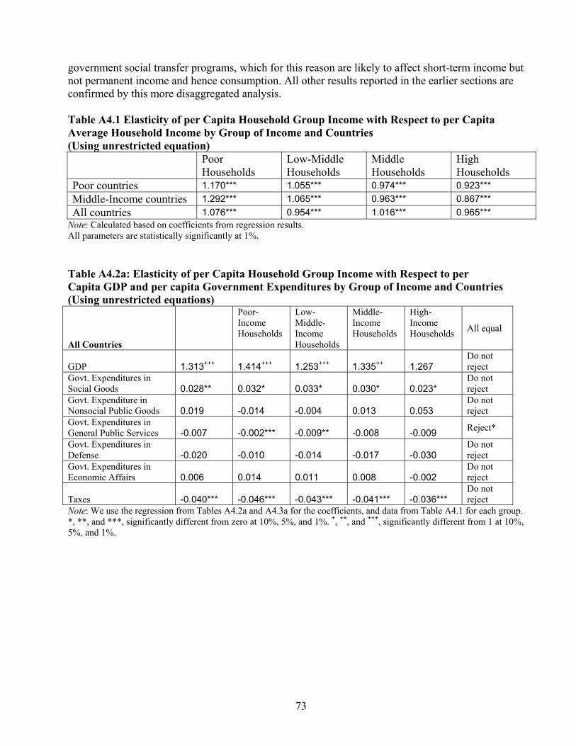
73
government social transfer programs, which for this reason are likely to affect short-term income but not permanent income and hence consumption. All other results reported in the earlier sections are confirmed by this more disaggregated analysis. Table A4.1 Elasticity of per Capita Household Group Income with Respect to per Capita Average Household Income by Group of Income and Countries (Using unrestricted equation)
Poor Households
Low-Middle Households
Middle Households
High Households
Poor countries 1.170*** 1.055*** 0.974*** 0.923*** Middle-Income countries 1.292*** 1.065*** 0.963*** 0.867*** All countries 1.076*** 0.954*** 1.016*** 0.965***
Note: Calculated based on coefficients from regression results. All parameters are statistically significantly at 1%. Table A4.2a: Elasticity of per Capita Household Group Income with Respect to per Capita GDP and per capita Government Expenditures by Group of Income and Countries (Using unrestricted equations)
All Countries
Poor-Income Households
Low-Middle-Income Households
Middle-Income Households
High-Income Households All equal
GDP 1.313+++ 1.414+++ 1.253+++ 1.335++ 1.267 Do not reject
Govt. Expenditures in Social Goods 0.028** 0.032* 0.033* 0.030* 0.023*
Do not reject
Govt. Expenditure in Nonsocial Public Goods 0.019 -0.014 -0.004 0.013 0.053
Do not reject
Govt. Expenditures in General Public Services -0.007 -0.002*** -0.009** -0.008 -0.009 Reject*
Govt. Expenditures in Defense -0.020 -0.010 -0.014 -0.017 -0.030
Do not reject
Govt. Expenditures in Economic Affairs 0.006 0.014 0.011 0.008 -0.002
Do not reject
Taxes -0.040*** -0.046*** -0.043*** -0.041*** -0.036*** Do not reject
Note: We use the regression from Tables A4.2a and A4.3a for the coefficients, and data from Table A4.1 for each group. *, **, and ***, significantly different from zero at 10%, 5%, and 1%. +, ++, and +++, significantly different from 1 at 10%, 5%, and 1%.

74
Table A4.2b Elasticity of per Capita Household Group Income with Respect to per Capita GDP and per Capita Government Expenditures by Group of Income and Countries (using unrestricted equations)
Poor Countries
TOTAL Household per Capita Income
Poor-Income Households
Low-Middle-Income Households
Middle-Income Households
High-Income Households All equal
GDP 1.134 1.326++ 1.196 1.105 1.046 Reject** Govt. Expenditures in Social Goods 0.013** 0.010* 0.012* 0.012* 0.015*
Do not reject
Govt. Expenditure in Nonsocial Public Goods -0.002 -0.014 -0.009 -0.006 0.010
Do not reject
Govt. Expenditures in General Public Services 0.011 0.021*** 0.017** 0.013 0.002 Reject*
Govt. Expenditures in Defense. -0.006 -0.001 -0.003 -0.004 -0.012
Do not reject
Govt. Expenditures in Economic Affairs 0.008 0.008 0.008 0.009 0.006
Do not reject
Taxes -0.038*** -0.042*** -0.040*** -0.038*** -0.034*** Do not reject
Middle-Income Countries
Poor-Income Households
Low-Middle-Income Households
Middle-Income Households
High-Income Households All equal
GDP 1.649++ 2.130++ 1.757+ 1.588+ 1.429 Do not reject
Govt. Expenditures in Social Goods -0.039 -0.025** -0.040** -0.046 -0.037
Do not reject
Govt. Expenditure in Nonsocial Public Goods 0.041 0.024 0.031 0.039 0.055 Reject*
Govt. Expenditures in General Public Services 0.029 0.043 0.036 0.031 0.016
Do not reject
Govt. Expenditures in Defense 0.004* 0.003 0.005 0.006 0.002**
Do not reject
Govt. Expenditures in Economic Affairs 0.002 0.004 0.006 0.006 -0.004
Do not reject
Taxes -0.096*** -0.122*** -0.109*** -0.102** -0.072** Do not reject
Note: We use the regression from Tables A4.2a’ and A4.3a for the coefficients, and data from Table A4.1 for each group. *, **, and ***, significantly different from zero at 10%, 5%, and 1%. +, ++, and +++, significantly different from 1 at 10%, 5%, and 1%.

75
Table A4.3a Regression Results Dependent Variable: Rate of Growth of Group per Capita Household Income Measured by Income Surveys
Poor Low-Middle Middle High Per Capita Govt. Expenditure 0.058* 0.072 0.051 -0.138 in Social Public Goods [0.034] [0.075] [0.191] [0.628] Per Capita Govt. Expenditure 0.071*** 0.146*** 0.301** 0.741** in Social Transfers [0.026] [0.052] [0.123] [0.372] Per Capita Govt. Expenditure -0.114 0.038 0.699 4.1 in Nonsocial Public Goods [0.122] [0.256] [0.663] [2.536] Per Capita Govt. Expenditure -0.037 -0.114** -0.222* -0.875** in Others (General Public Services, Defense, Economic Affairs)
[0.024] [0.050] [0.125] [0.402]
Per Capita Taxes -0.054*** -0.097*** -0.193** -0.410* [0.017] [0.032] [0.076] [0.230] Growth in per Capita GNI 0.275*** 0.504*** 0.944*** 2.135*** [0.063] [0.117] [0.270] [0.766] Growth in per Capita Debt -0.110** -0.164* -0.590*** -3.046*** [0.047] [0.096] [0.218] [0.550] Observations 58 58 58 58 Standard errors in brackets; regression includes time-restricted dummies Countries: 37 For government expenditure we use country dummies as instruments, for GNI growth we add political and demographic variables; we assume growth in debt is not endogenous. * significant at 10%; ** significant at 5%; *** significant at 1%

76
Table A4.3b Regression Results Dependent Variable: Rate of Growth of per Capita Group Consumption Measured in Household Consumption Surveys
Poor Low-Middle Middle High Per Capita Govt. Expenditure 0.022 0.05 0.087 0.361 in Social Public Goods [0.057] [0.108] [0.197] [0.634] Per Capita Govt. Expenditure -0.008 -0.009 -0.016 -0.012 in Social Transfers [0.016] [0.028] [0.050] [0.144] Per Capita Govt. Expenditure -0.053 -0.074 -0.039 0.323 in Nonsocial Public Goods [0.105] [0.190] [0.343] [1.107] Per Capita Govt. Expenditure 0.057*** 0.100*** 0.150*** 0.198 in Others General Public Services, Defense, Economic Affairs)
[0.016] [0.029] [0.050] [0.146]
Per Capita Taxes -0.070*** -0.129*** -0.220*** -0.571*** [0.016] [0.028] [0.050] [0.156] Growth in per Capita Household 0.479*** 0.816*** 1.369*** 3.955*** Final Consumption Expenditure from National Accounts
[0.071] [0.112] [0.194] [0.594]
Growth in per Capita Debt 0.029 0.032 0.025 -0.3 [0.045] [0.078] [0.132] [0.361] Observations 80 80 80 80 Standard errors in brackets; regression includes time-restricted dummies Countries: 37 For Government Expenditure we use country dummies as instruments; for Household Expenditure growth we add political and demographic variables; we assume growth in debt is not endogenous. * significant at 10%; ** significant at 5%; *** significant at 1%

77
Table A4.4a Elasticity of per Capita Household Group Income or Consumption with Respect to Per Capita Household Expenditure from National Accounts and per Capita Government Expenditures (Using unrestricted equations)
Income Survey
TOTAL Household per Capita Income
Poor-Income Households
Low-Middle-Income Households
Middle-Income Households
High-Income Households
GNI 1.269*** 1.582*** 1.389*** 1.401*** 1.001*** Social Public Goods Exp. 0.005 0.024* 0.014 0.005 -0.005 Social Transfers 0.033** 0.034*** 0.033*** 0.037** 0.029** Nonsocial Public Goods Exp. 0.027 -0.017 0.003 0.027 0.049 Other Expenditures -0.033** -0.021 -0.030** -0.032* -0.040** Taxes -0.038*** -0.047*** -0.041*** -0.043** -0.029*
Consumption Survey
TOTAL Household per Capita Consumption
Poor-Income Households
Low-Middle-Income Households
Middle-Income Households
High-Income Households
Final Household Expenditure from National Accounts 1.494*** ++ 1.355*** + 1.335*** + 1.426*** ++ 1.755*** +++ Social Public Goods Exp. 0.011 0.007 0.009 0.010 0.017 Social Transfers -0.002 -0.003 -0.002 -0.002 -0.001 Nonsocial Public Goods Exp. -0.001 -0.008 -0.007 -0.002 0.008 Other Expenditures 0.032*** 0.037*** 0.038*** 0.036*** 0.020 Taxes -0.065*** -0.057*** -0.060*** -0.065*** -0.072***
Note: We use the regression from Tables A4.2a’ and A4.3a for the coefficients, and data from Table A4.1 for each group. *, **, and ***, significantly different from zero at 10%, 5%, and 1%. +, ++, and +++, significantly different from 1 at 10%, 5%, and 1% (this is only tested for Household Expenditure and GNI elasticities)
Table A4.4b Wald Tests of Difference of Elasticities by Income Group
Income Survey Income Survey All Equal
Consumption Survey All Equal
GNI Do not reject Do not reject
Social Public Goods Exp. Do not reject Do not reject Nonsocial Public Goods Exp. Reject* Do not reject
Transfers Do not reject Do not reject
Other Expenditures Do not reject Do not reject Taxes Do not reject Do not reject
Note: *, **, *** reflect significance at 10, 5, and 1 percent, respectively.

78
Annex 5 Fiscal Policy and the Environment Summary of Background Paper 3 18 Introduction This annex is based on López and Islam (background paper 3) analyzing how the level and composition of government expenditures affect air pollution. Following the framework in annex 2, this paper focuses on the public goods versus private goods (or nonsocial subsidies) composition of government expenditures. The central hypothesis is that, ceteris paribus, increasing the provision of public goods is in general good for the environment as it tends to make the economy less environmentally demanding, especially under conditions of market failure. Credit market failure and the existence of environmental externalities are key market failures in developing countries. As López and Galinato (2007) show, credit market imperfections affect much more the level of the economy’s investment in human capital than in physical capital. This implies that an economy affected by credit market failure is likely to have a human to physical capital ratio that is too low. Thus, economies affected by large credit-market imperfections tend to specialize in physical capital-intensive activities instead of human capital-intensive activities. Under the plausible assumption that physical capital-intensive activities are dirtier and more environmentally demanding than human capital-intensive activities, we can conclude that unmitigated credit-market failure tends to make the economy more pollution intensive. That is, such economies have greater pollution to output ratios. Governments that provide more public (social) goods will tend to raise the level of human capital and thus the structure of production of the economy may shift toward human capital-intensive activities, which are generally cleaner than physical capital-intensive activities. By contrast, government expenditures in private goods or nonsocial subsidies tend to be captured by the wealthy, who usually own and control most of the physical capital of the economy. These subsidies either increase the consumption of the elites or help raise their investment in physical capital. Thus a shift of government expenditures from private to public goods is likely to make the economy more human capital intensive and thus cleaner.19 Similarly, the private sector will tend to overpollute and underinvest in the protection of the environment because of environmental externalities. Governments that emphasize the provision of public goods will tend to spend more resources in developing and improving institutions (an important
18 Based on a background paper prepared by Ramón López and Asif Islam. 19 The role of the structure of government expenditures on pollution is likely to be more important in low- and middle-income (less developed) countries (LDCs) than in developed countries. The reason is that the market failures tend to be more pronounced in LDCs than in developed countries. Also, the impact of credit-market failure is greater the larger the proportion of the population that is poor. In LDCs, a larger portion of the population is dependent on government expenditures in government-provided public goods (particularly education, health, and social transfers) than developed countries and therefore the effect of government expenditures in public goods on the level of human capital of the economy is likely to be much larger in LDCs than in developed countries. Consequently, the impact on pollution of the composition of government expenditures is also likely to be more pronounced in LDCs than in developed countries.

79
public good), including environmental institutions, and to invest more in protecting natural habitats (also important public goods). Compared to earlier studies, the present study considers explicitly the composition of government expenditures on environmental quality using a comprehensive set of air pollution indicators. We also examine the scale and income effects on pollution. We use household final consumption expenditure as a measure of the income instead of GDP per capita income. We also consider multiple pollutants and political controls (democracy measure). In addition, we explicitly allow for an economic growth effect in addition to the usual scale and income effects. This reflects the hypothesis that as the speed of economic growth accelerates environmental regulation and institutions to control environmental damage encounter increasing difficulties to adapt quickly enough to respond adequately to the challenges induced by a faster-growing economy. Thus, we use the rate of growth of GDP in addition to the level of GDP per capita and household per capita income as an additional factor affecting the environment. The Data and the Estimating Model We use a recently updated data set called Global Environmental Monitoring System (GEMS) for the period 1986–99 for five air pollutants: sulfur dioxide, nitrogen dioxide, air particles (particulate matter of 10 microns in diameter or smaller; PM10), lead, and carbon monoxide. These data consist of actual measurement of the pollutant concentration in the air in fixed sites distributed in a large number of cities. There are about 1,128 observations20 distributed in 86 cities with about 2.5 measurement sites per city per year, on average. The total number of countries included in the sample is 31, of which 19 are low and middle income and 12 are considered developed according to the World Bank classification. The rest of the data used comes from standard national account sources with the exception of a trade openness indicator (ASATI) constructed by the authors and the government expenditure data, which comes from Government Financial Statistics sources (see Table A5.1 for a full description of the variables and data used). We estimate the effect of the government expenditure variables controlling for a number of variables often used in the literature that estimates pollution. The two key government expenditure variables are the total government expenditures and the share of expenditures in public goods on total government expenditures. The effects of the level and composition of government expenditures on the various air pollutants considered is the focus of the analysis. The most important control variables are related to the scale of economic activity, economic growth, and the level of (permanent) income per capita, which appear as distinct variables in the ensuing regressions. In contrast with most early studies that have used GDP per capita as a single measure of output scale, per capita wealth, and economic growth, we separate these three effects by using appropriate indicators. Previous studies often use nonlinear polynomial transformations of per capita GDP to deal with the potentially conflicting effects of scale, wealth, or permanent income effect and growth effect on demand for clean air (which is of course the inverse of air pollution). Instead of playing with polynomial transformations of per capita GDP to account for the conflicting directions of the three effects mentioned earlier, we choose to separate the three effects through appropriate 20 These numbers correspond to sulfur dioxide observations included in the weighted OLS regression, which are the most numerous. For other pollutants there are fewer observations.

80
variables. There are two advantages to this over the conventional approach: (1) Our approach allows us to go beyond the black box effects and identify the three effects, and (2) our approach avoids the econometric disadvantages of using the various polynomial transformations of the same variable in the same regression, including colinearity of the variables, questions on the stability of such coefficients, and others. The scale of economic activity is measured by country GDP per square kilometer to give an idea of the output scale pressure on the natural environment. The level of per capita wealth or permanent income is represented by a national account measure of household final consumption expenditure per capita as an indicator of the level of household wealth. As is well known, per capita household consumption is a better measure of wealth or permanent income than per capita income. In addition, to better capture the permanent income or wealth effect on the demand for clean air we use the average three-year period of per capita household consumption as a regressor instead of merely the current consumption. The idea is that GDP as a measure of physical output is likely to have a different effect on the environment than the level of household wealth. Increasing output (ceteris paribus) is likely to cause more environmental pressure, while increasing wealth is likely to cause consumers to increase their demand for environmental amenities, including cleaner air. To the extent that governments are at least in part responsive to this demand, increasing household wealth may have the effect of reducing pollution; that is, the opposite effect of GDP level. We also control for the rate of GDP growth to capture the fact that growth itself as opposed to the level of GDP may have a more negative effect on the environment; that is, two countries with the same level of GDP and wealth per capita but different growth rates will have different impacts on the environment. This is a dynamic effect that depends upon the speed by which environmental institutions and regulation evolve over time versus the speed by which the demands upon the environment occur. The faster the rate of growth of GDP is the more difficult it will be for the environmental institutions to adapt at the required pace to counter some of the negative impact of output scale on the environment. Thus, we expect that the rate of economic growth exerts a negative effect on the environment (i.e., that pollution is likely to be increasing with the speed of growth). In addition, we use measures of economic openness, taxes, and investment as further control variables. The regressions use all variables in log form using the site measurement (instead of the city average or even the country mean) as a unit of observation. We first provide OLS estimates. A major concern of course is the possibility of biases of the OLS coefficients. These biases can arise especially from omitted variables caused by the existence of unobserved characteristics of the cities and sites themselves.21 To deal with these potential problems we control for unobserved effects through fixed effects and, alternatively, through random effects. We control for fixed site effects, which are the basic units of observation using fixed effect (FE) estimators. A problem with the FE estimators, however, is that they rely exclusively on the time variance and do not use the important information embodied in cross-site variance. For this reason we also use random effects (RE) controlling for certain site characteristics that are observable as well as for city or country effects (these are often referred to as
21 There is also a possibility of biases caused by reverse causality. Most of the explanatory variables, however, are macro in nature and are thus highly unlikely to be affected by the levels of specific air pollutants. Furthermore, a very small fraction of government expenditures in the sample are toward the environment. In general, there has been a degree of implicit consensus in the literature in this respect. Antweiler, Copeland, and Taylor (2001), for example, do not consider reverse causality to be an issue.

81
quasi-fixed effects). Essentially we look to probe for the stability of the coefficients, mainly those that relate pollution to the structure of public expenditures. Results We first get the weighted OLS estimates for the five air pollutants considered. The OLS estimates explain between 40 percent and 50 percent of the total variance of the air pollutant concentrations measured. The effect of the share of public goods in total expenditures is negative and significant for all pollutants, with the exception of only PM10, which has a positive and significant coefficient. That is, these estimates suggest that the structure of fiscal expenditures may be an important determinant of pollution and, in general, the greater the participation of expenditures of public goods (and the lower the participation of nonsocial subsidies) in government expenditures the better air quality is as measured by the air concentrations of sulfur dioxide (SO2), nitrogen dioxide (NO2), carbon monoxide (CO), and lead. In addition, these estimates generally conform to a priori expectations regarding the other explanatory variables. Per capita household wealth has a generally negative effect on most pollutants, with the exception of NO2, where the effect appears to be not significantly different from zero. The output-scale effect tends to be positive, with the exception of CO, and the rate of economic growth tends to have a positive effect on the pollutants. Trade openness has a mostly negative and significant effect on the pollutants. Estimates from the two-way fixed effects (TWFE), where we control for site effects as well as common time effects, show that in general the TWFE affects the magnitude of the coefficients but generally confirm the sign and statistical significance of almost all of them. In addition, the explanatory power of the regressions increases dramatically vis-à-vis the OLS estimates by almost 80 percent. These results confirm the generally negative effect of the share of public goods in government expenditures on all pollutants, with the exception of PM10, as was also the case of the OLS estimates. While the sign of the other four coefficients is still negative, the statistical significance remains for the SO2 and lead coefficients but not for NO2 and CO coefficients. The effects of the remaining controls also tend to be confirmed, and in some cases these results are even sharpened. In particular, the consistent, significant, and negative effect of trade openness on all pollutants is quite remarkable. Table A5.2 shows TWFE but now also controlling for certain political variables that may affect the emergence and enforcement of environmental regulation. We use an indicator of freedom of the press, another of institutional quality (Polity 2), and another one that measures the number of years under democratic stability. The first one is likely to be associated with civil controls upon the government, which could induce governments to be more responsive to demands for environmental quality of the population. We thus expect a negative effect of this variable on pollution. The same is true for the stability of democracy and Polity 2, which may also be correlated with the ability of governments to develop and apply adequate environmental protection. In general, the TWFE estimators are mainly maintained when we control for these political variables, with SO2 and lead levels still strongly and negatively influenced by the propensity of the government to spend in public goods instead of private ones. The variable freedom of the press seems to be strongly related to lower pollution levels, as expected. Estimates obtained using RE methods confirm those obtained using TWFE methods, except that now the effect of the share of public goods is sharper, showing a negative and significant effect not only on the levels of SO2 and lead as in the case of the TWFE estimators but in addition capture a negative and significant effect of the share of public goods on NO2. In Table A5.3 we report RE estimators

82
using controls for measurable site characteristics (which can be called quasi-fixed-effects estimators) such as whether the measurement sites are located in a city center, industrial locations, or areas subject to heavy traffic vis-à-vis low traffic areas. The results are still highly consistent with the earlier ones obtained using FE, with the levels of SO2, NO2, and lead all negatively and significantly affected by the share of public goods in government expenditures. Hausman tests performed show that both RE estimators for NO2 are unbiased vis-à-vis the corresponding TWFE estimators. The Hausman tests are, however, rejected for PM10, CO (for RE specification with site controls), SO2, and lead, suggesting that for these equations the TWFE estimators should be preferred. One may also argue that the RE-site controlling estimators should be preferred to the TWFE estimators in the case of SO2, CO, lead, and PM10. Thus, based on the Hausman test, we can conclude that the “best” estimates for the determinants of the level of NO2 is the RE one, while the TWFE ones are to be preferred for the other four pollutants. Using the “best” estimates (RE quasi-fixed effect for NO2, TWFE estimators with political controls for SO2, lead) we performed a simulation of the effect of changes in the share of public goods on the air concentrations of SO2, NO2, and lead. Increasing the share of public goods by one standard deviation (about 30 percent of the sample mean) reduces SO2 concentrations by 16 percent of its standard deviation (18 percent of the sample mean), NO2 pollution by 12 percent of its standard deviation (7 percent of the sample mean), and lead by 13 percent of its standard deviation (or 22 percent of the sample mean). These are very substantial effects indeed, implying elasticities of the order of 0.6, 0.2, and 0.7, respectively. The main conclusion is that the structure of government expenditures is an important determinant of air quality. Increasing the participation of public goods vis-à-vis private goods in government expenditures contributes to significantly reducing SO2, NO2, and lead pollution. The negative and highly robust effect of the share of public goods is very important, mainly because SO2 is arguably the most important air pollutant, is the pollutant for which the measurement technologies are the most perfected, and is the pollutant for which the available data is most complete. This gives us great confidence in this result. The only pollutant that appears to be positively related to the share of public goods is PM10.

83
Table A5.1 Description of Variables
Variable Description Years Available
Source
Sulfur Dioxide (SO2) SO2 concentration, micrograms per cubic meter 1986–99 GEMS Nitrogen Dioxide (NO2) NO2 concentration, micrograms per cubic meter 1986–99 GEMS Particulate Matter 10 (PM10)
PM10 concentration, micrograms per cubic meter 1986–99 GEMS
Lead Lead, micrograms per cubic meter 1986–99 GEMS Carbon Monoxide CO concentration, milligrams per cubic meter 1986–99 GEMS Household Final Consumption Expenditure per Capita (2000 US$)
Household Final Consumption Expenditure (formerly private consumption) is the market value of all goods and services, including durable products (such as cars, washing machines, and home computers), purchased by households. It excludes purchases of dwellings but includes imputed rent for owner-occupied dwellings. It also includes payments and fees to governments to obtain permits and licenses. Here, household consumption expenditure includes the expenditures of nonprofit institutions serving households, even when reported separately by the country.
1980–2004 World Development Indicators (World Bank)
GDP Growth (2000 US$) Real GDP per Capita Growth (constant US$ 2000)
1980–2004 World Development Indicators (World Bank)
Share of Govt. Exp. in Public Goods
This is the Share of Government Expenditure on Public Goods. Public goods are defined as a total of the following: i) Education ii) Health iii) Social security iv) Transport v) Communication vi) Public order and safety vii) Housing and community amenities viii) Environmental protection ix) Religion and culture
1980–2004 Government Financial Statistics (IMF), Asian Development Bank, country data
Trade Openness Sati index, which is the residual of the regression of Trade on population, area, GDP per capita, dummy for industrialized country, dummy for oil exporter, and imports over export prices. A positive residual implies a more open economy.
1980–2001 Pritchett, Lant 1996. Updated by López and Galinato (2007)
GDP per Square Km Total GDP (2000 US$) over land area. 1980–2004 World Development Indicators (World Bank)
Share of Govt. Exp. over GDP
1980–2004 Penn World Tables (2006)
Share of Investment over GDP
1980 –2004 Penn World Tables (2006)
Polity Index (Polity 2)
Score that indicates how democratic a country is. 1980–2003 Polity IV www.cidm.umd.edu

84
Table A5.2 Two-Way Fixed Effects Regression Results with Site and Year Effects Controlling for Political Variables (Pollutants in Natural Log Form)
SO2 NO2 CO PM10
Lead
Log of Household Final Consumption -0.075 0.266 -3.305*** -3.491*** 2.120** Expenditure per Capita (2000 US$), average of current and previous two years
[0.594] [0.620] [0.976] [0.734] [1.061]
Log of Total GDP (2000 US$) over 0.321 0.411 3.059*** 3.134*** -0.627 Land area (sq km) [0.527] [0.592] [0.942] [0.753] [1.106] Growth Rate of GDP 1.528*** 0.703 -0.581 -1.038 3.207*** [0.573] [0.591] [0.665] [0.737] [1.042] Share of Public Goods (as -1.099*** 0.034 0.577* 1.734*** -1.344*** % of total gov’t exp) [0.313] [0.232] [0.313] [0.423] [0.496] Share of Government Consumption Expenditure -2.176 1.848 3.224** -6.604*** -9.712* Over GDP—Penn Tables [1.734] [1.578] [1.623] [2.270] [5.335] Trade—ASATI Index -0.003 0.002 -0.005** -0.011*** -0.008** [0.002] [0.002] [0.002] [0.003] [0.004] Share of Investment over GDP 0.126 0.151 -0.164 -3.352** -4.253** [1.001] [0.969] [1.007] [1.470] [2.001] Dummy Freedom of Press -0.329*** -0.254*** -0.112 -0.018 -0.222* [0.049] [0.059] [0.086] [0.057] [0.123] Polity 2 -0.038 -0.022 -0.093*** -0.019 -0.031 [0.025] [0.019] [0.021] [0.020] [0.023] Years of Democratic Stability 0.052 -0.017 0.084 0.131 0.003 [0.052] [0.043] [0.056] [0.132] [0.068] Tax/GDP 0.018*** 0.013** 0.03 -0.531 1.211 [0.005] [0.006] [0.073] [0.568] [0.865] Constant 1.939 -3.252 2.988 -7.505 -2.956 [3.546] [2.870] [3.673] [7.000] [8.792] SITE DUMMY YES YES YES YES YES YEAR DUMMY YES YES YES YES YES Observations 1128 994 663 573 457 Adjusted R-squared 0.91 0.88 0.95 0.81 0.93 Notes: Robust standard errors in brackets; regressions weighted by number of observations per county. * significant at 10%; ** significant at 5%; *** significant at 1%

85
Table A5.3 Random Effects Regression Results with Year Dummies and Site Characteristics (Pollutants in Natural Log Form)
SO2 NO2 CO PM10
Lead
Log of Household Final Consumption Expenditure per Capita (2000 US$), average of -0.248*** 0.137*** -0.628*** -0.580*** -0.667*** current and previous two years [0.077] [0.053] [0.114] [0.042] [0.117] Log of Total GDP (2000 US$) over 0.157*** 0.026 -0.086** 0.091*** -0.079 Land area (sq km) [0.045] [0.026] [0.041] [0.021] [0.060] Growth Rate of GDP 1.709*** 1.246*** 1.520*** 0.604 2.331*** [0.439] [0.341] [0.417] [0.460] [0.812] Share of Public Goods (as -1.144*** -0.408*** 0.063 1.208*** -0.763* % of total gov’t exp) [0.193] [0.156] [0.199] [0.272] [0.410] Share of Government Consumption Expenditure -5.082*** -2.505*** -1.696 -2.297*** -15.831*** Over GDP—Penn Tables [1.096] [0.686] [1.145] [0.709] [1.969] Trade—ASATI Index -0.006*** -0.001 -0.005*** -0.004** -0.015*** [0.002] [0.001] [0.001] [0.002] [0.003] Share of Investment over GDP -0.07 -0.496 -0.067 0.049 -5.181*** [0.590] [0.579] [0.641] [0.420] [1.125] Tax/GDP 0.0002 0.004 0.001 -0.104* 0.402 [0.003] [0.003] [0.005] [0.053] [0.362] Former Socialist Dummy 0.27 0.502*** -1.035*** -0.223* 0.157 [0.248] [0.126] [0.257] [0.121] [0.343] City Center Dummy -0.035 0.107 0.297** -0.061 0.178 [0.115] [0.066] [0.122] [0.071] [0.229] Other Urban Dummy -0.278** -0.151* -0.247* -0.006 -0.056 [0.141] [0.089] [0.133] [0.093] [0.219] Traffic Dummy 0.395*** 0.524*** 0.873*** dropped 1.564*** [0.146] [0.122] [0.204] [0.377] Constant 4.373*** 2.939*** 14.031*** 7.160*** 8.353*** [0.661] [0.441] [0.856] [0.503] [1.138] YEAR DUMMY YES YES YES YES YES Observations 1128 994 663 573 457 No. of Sites 220 191 128 117 90 Hausman Test Chi-square (P-value)
41.75 (0.002)
11.37 (0.911)
85.52 (0.000)
192.45 (0.000)
25.69 (0.080)
Within R-squared 0.40 0.08 0.38 0.10 0.73 Between R-squared 0.30 0.37 0.50 0.68 0.41 Overall R-squared 0.35 0.36 0.42 0.60 0.38 Robust standard errors in brackets * significant at 10%; ** significant at 5%; *** significant at 1%

86
Annex 6 Summary of the Country Studies 6.1: Brazil and the Quality of Growth: Government Expenditures and Tax Revenues, 1990–2005 Summary of Country Case Study22 Over the last decade and a half, tax revenues and expenditures in Brazil have been growing faster than GDP. Tax revenues have increased at a faster rate than government expenditures, excluding expenses with the debt service, while debt service itself also increased significantly. Moreover, there has been a significant change in the allocation of government expenditures, with remarkable increases in social expenditures and decreases in investment. The combination of higher tax revenues and expenditures, together with the changes in the allocation of expenditures, has had important implications for Brazil (see figure A6.1.1 and 6.1.2). The picture that emerges from this analysis is of a country that has grown at relatively low rates, but where the well-being of the population has improved via decreases in inequality in many aspects, be it in income, education, health, or regional and racial disparities. Brazil is an exceptional case in the growth-poverty-inequality nexus, because improvement in the income distribution translated into poverty reduction, despite the lack of income growth. Since the 1990s, Brazilian economic growth has been highly unstable and, on average, relatively low, especially if growth rates are compared to those of other “emerging” countries. In the past 10 years, the average annual real per capita GDP growth was 0.5 percent. Poverty and inequality are still relatively high but have been decreasing. According to estimates using regional poverty lines, poverty incidence decreased from 38 percent to 34 percent between 1995 and 2004; extreme poverty from 28 percent to 22 percent, and both measures continued to decrease even more sharply between 2004 and 2006 (figure A6.1.3). Inequality has been significantly reduced more recently, as indicated by the Gini coefficient, which decreased from about 0.59 in the late 1990s to 0.56 in 2005, a remarkable reduction that is rarely observed in other countries. This improvement in equality has been attributed mainly to the fact that economic activity has increased in geographical disadvantaged areas, to higher- and better-targeted social assistance and better-distributed education. Despite its importance, the effect of taxes for income distribution has not been analyzed recently in Brazil, but some studies indicate that the nominal incidence of net taxes has become more regressive in the past 10 years because of the increased importance of indirect taxes. Table A6.1.1 shows that while direct tax was progressive, indirect tax is regressive and increasing. From 1996–2004, the tax incidence has increased by 20 percentage points for families earning up to two times the minimum wage, but rose only 8.4 percentage points for richer families earning more than 30 times the minimum wage.
22 Based on a background paper prepared by Claudia Romano and Sergio Sakurai.

87
Table A6.1.1 Direct, Indirect, and Total Tax Incidence on Family Income in 1996 and 2004 % of Family Income
Direct tax Indirect tax Total tax Change in Tax Incidence 1996–2004 (in percentage points)
Monthly Family Income (minimum wages; MW) 1996 2004 1996 2004 1996 2004 Up to 2 MW 1,7 3,1 26,5 45,8 28,2 48,8 20,6 2 to 3 2,6 3,5 20,0 34,5 22,6 38,0 15,4 3 to 5 3,1 3,7 16,3 30,2 19,4 33,9 14,5 5 to 6 4,0 4,1 14,0 27,9 18,0 32,0 14,0 6 to 8 4,2 5,2 13,8 26,5 18,0 31,7 13,7 8 to 10 4,1 5,9 12,0 25,7 16,1 31,7 15,6 10 to 15 4,6 6,8 10,5 23,7 15,1 30,5 15,4 15 to 20 5,5 6,9 9,4 21,6 14,9 28,4 13,5 20 to 30 5,7 8,6 9,1 20,1 14,8 28,7 13,9 More than 30 MW 10,6 9,9 7,3 16,4 17,9 26,3 8,4 Source: Primary data: Instituto Brasileiro de Geografia e Estatistica (Brazilian Institute for Geography and Statistics), POF 1995/6, POF 2002/3; Vianna et al. (2000); SRF (Secretary of Federal Revenue), “A progressividade no consumo—tributação cumulativa e sobre o valor agregado.” Apud, Zockun et al. (2007). Note: Indirect taxes obtained from POF applying nominal rates to consumption: Imposto sobre Produtos Industrializados[tax on Industrial Products], Imposto sobre Circulação de Mercadorias e Serviços (Tax on Movement of Goods and Services) , Programa de Integração (Social Integration Program), Contribuição para Fin Social; Direct taxes obtained directly from POF: Income tax, labor-related taxes, Imposto sobre Propriedade de Veiculos Automotores (Tax on Motor Vehicle Owners) Imposto Predial e Territorial Urbano (Urban and Territorial Land Tax); Imposto sobre Serviços (Service Tax): Authors calculations. On the other hand, there has been increased government enforcement of tax collection, reduction of tax evasion and lower household-income tax exemptions, all of which may be positively affecting income distribution since these disproportionately benefit the rich rather than the poor. Between 1991 and 2005, income tax alone increased from 8 percent to 16 percent of GDP, while in the same period the share of indirect taxes increased from 11 percent to 18 percent of GDP (figure A6.1.4). Various studies show that income taxes are progressive in Brazil; therefore, their increase is likely to improve income distribution. There has been also a gradual but steady decrease in household income tax exemptions, from 0.56 percent of GDP in 1998 to 0.44 percent of GDP in 2005; even if not large, this change may also have a positive effect on income distribution. The net effect of all these developments remains to be analyzed. On the fiscal expenditure side, spending public goods increased slightly from about 16 percent to 19 percent of GDP between 1991 and 2005, while spending on private goods have been unstable, but in 2005 its share of GDP was the same as it was in 1991 (figure A6.1.5). Most of the private expenditures come from the retirement and pension system. Subsidies increased significantly until 2005. A significant proportion of the tax exemptions are allocated to industry and to the commerce and services sectors (38 percent of total in 2005). The single highest value is for the pension and retirement system. The share of spending on public goods in total expenditure was about 26 percent in 2005 (figure A6.1.2). Other areas, such as education and health, have also benefited from higher expenditures and have improved over the last 15 years. Elementary school enrollment, literacy, and average years of schooling have improved, while expenditures on education have increased by about 1 percent of GDP. Despite significant improvements in access to education, Brazil needs to invest in the quality of education, which has been even declining over time. Expenditures on health and sanitation have

88
doubled as a share of GDP over the last decade and a half and health indicators have improved; for instance, as measured by the infant mortality rates, which decreased from 48 to 28 deaths per 1,000 live births between 1990 and 2002. Sanitation is still a major problem, however, causing about 700,000 hospitalizations per year. Not only is sewage collection low (about 65 percent of households), but also a small proportion of what is collected is treated (about 35 percent of what is collected), while investments in sanitation continue to be much below the necessary level. One of the most important environmental problems in Brazil continues to be Amazon deforestation, which has negative effects not only related to the loss of biodiversity, soil and water quality, and climate regulation, but also because it is the most important cause of carbon emissions in Brazil (deforestation and land use change make up 75 percent of total emissions). While deforestation rates in the Amazon were stable between 1996 and 2001, the average rate increased again in the three years between 2002 and 2004, reaching the peak of 27,000 square kilometers in 2004; only decreasing again in 2005/6. Nowadays there are few federal government incentives for land use expansion in the Amazon, but logging and large-scale agriculture and pasture still exert great pressure over the area. The government’s strong interest in making Brazil a producer of ethanol, and rising prices for soybeans and meat, are causing renewed concerns that there will be a new rush for land use and higher Amazon deforestation. Indeed, preliminary deforestation figures for 2007 indicate a significantly increased rate of deforestation in the Amazon. Despite its importance for carbon emission and biodiversity, as well as for soil and water quality, the level of spending in the control of land use in the Amazon is significantly lower than necessary, and whatever is allocated is not used efficiently The analysis here indicates that Brazil’s fiscal policy has the characteristics of type B interventions. Though interventions have been moving closer to type A over the last decade, the tax system is still mainly based on indirect taxes and the system of nonsocial subsidies is still in place. The expenditure policy has shown an increase in the allocation of spending on public goods, especially on social services. Expenditure on provision of public goods accounted for over 20 percent of GDP, or 45 percent of government expenditure. Therefore, we consider that the structure of public expenditures has the characteristics of type A interventions related to social spending. But implementation of environmental policy can be classified as type B, as despite not having direct incentives for environmental degradation, investment in deforestation control and sanitation are significantly lower than the need for investments. In sum, Brazil is experiencing a significant decrease in poverty and a clear improvement in income distribution, in part thanks to the improvement in the composition of expenditure, although long-run structural change may have played a role. Economic growth, however, has not yet increased from the levels of the 1990s, though there are recent indications that it may be entering a period of faster growth since 2006. In order for Brazil to continue on this positive path, many challenges need to be confronted and issues need to be resolved, including, for example, the social assistance programs that need to be integrated with social policies that allow for a more sustainable path out of poverty, and with the structural reforms needed for faster economic growth, as well as the need for more investment in infrastructure and a more efficient tax system.

89
Figure A6.1.1 Brazil: Composition of Government Expenditure in GDP (all levels of governments)
0
5
10
15
20
25
30
1991 1993 1995 1997 1999 2001 2003 2005
% o
f GD
P
Social assistance and pension and retirement systemEducation and cultureHealth and sanitationOthersAdministration, Planning, Legislative and Judiciary
Source: Secretaria do Tesouro Nacional (Secretary of the National Treasury). Note: 1990–2005: all levels of governments are included. Exchange rate: 1US$ = R$2.10; all values are adjusted by using the Indice Nacional de Preços ao Consumidor Amplo (IPCA) price index—R$ of 2006. Figure A6.1.2 Brazil: Share of Expenditure on Public versus Private Goods (all levels of governments)
0
5
10
15
20
25
30
1991 1993 1995 1997 1999 2001 2003 2005
% o
f GD
P
Public Private Subsidies Undefined
Source: Secretaria do Tesouro Nacional (Secretary of the National Treasury). Note: 1990–2005—all levels of governments are included; exchange rate: 1US$ = R$2.10; all values are adjusted by using the IPCA price index—R$ of 2006.
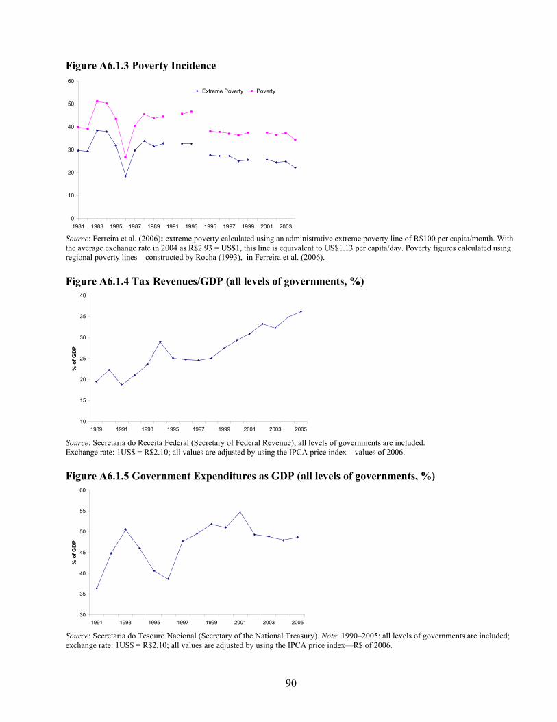
90
Figure A6.1.3 Poverty Incidence
0
10
20
30
40
50
60
1981 1983 1985 1987 1989 1991 1993 1995 1997 1999 2001 2003
Extreme Poverty Poverty
Source: Ferreira et al. (2006): extreme poverty calculated using an administrative extreme poverty line of R$100 per capita/month. With the average exchange rate in 2004 as R$2.93 = US$1, this line is equivalent to US$1.13 per capita/day. Poverty figures calculated using regional poverty lines—constructed by Rocha (1993), in Ferreira et al. (2006). Figure A6.1.4 Tax Revenues/GDP (all levels of governments, %)
10
15
20
25
30
35
40
1989 1991 1993 1995 1997 1999 2001 2003 2005
% o
f GD
P
Source: Secretaria do Receita Federal (Secretary of Federal Revenue); all levels of governments are included. Exchange rate: 1US$ = R$2.10; all values are adjusted by using the IPCA price index—values of 2006. Figure A6.1.5 Government Expenditures as GDP (all levels of governments, %)
30
35
40
45
50
55
60
1991 1993 1995 1997 1999 2001 2003 2005
% o
f GD
P
Source: Secretaria do Tesouro Nacional (Secretary of the National Treasury). Note: 1990–2005: all levels of governments are included; exchange rate: 1US$ = R$2.10; all values are adjusted by using the IPCA price index—R$ of 2006.

91
Table A6.1.2 Composition of Brazilian Tax Exemptions, by Type of Function Government Function 2003 2004 2005 US$ % US$ % US$ % Agriculture 385,716,514 2.77 275,776,327 1.33 351,530,571 1.70 Energy 0 0 7,965,061 0.04 145,658,340 0.70 Labor 89,486,993 0.64 1,023,641,183 4.93 1,576,458,303 7.63 Science and technology 146,649,312 1.05 291,675,897 1.40 310,875,289 1.50 Transport 87,792,781 0.63 153,055,106 0.74 129,246,253 0.63 Industry 3,585,572,997 25.78 3,030,471,247 14.59 3,838,503,481 18.57 Commerce and services 2,652,028,860 19.07 3,816,959,880 18.37 3,986,560,503 19.29 Education 357,188,218 2.57 585,100,059 2.82 875,019,429 4.23 Culture 201,235,636 1.45 141,522,623 0.68 233,316,670 1.13 Health 1,190,878,113 8.56 2,439,445,257 11.74 2,479,092,811 11.99 Housing 77,164,449 0.55 309,612,800 1.49 330,664,307 1.60 Social assistance 42,538,900 0.31 531,606,650 2.56 977,341,328 4.73 Pension and retirement system 5,081,562,621 36.54 8,171,150,756 39.33 5,426,179,217 26.25 Rural land organization 10,142,502 0.07 0 0 9,721,803 0.05 Total 13,907,957,896 100 20,777,982,845 100 20,670,168,307 100 Source: Secretaria da Receita Federal (Secretary of Federal Revenue) Note: Exchange rate: 1 US$ = R$2.10; all values are adjusted by using the IPCA price index—R$ of 2006.
=========================================================== 6.2 Chile and the Quality of Growth Summary of Country Study23 Chile has been cited as a successful case of development. Relatively fast economic growth over almost two decades has been accompanied by a significant reduction in absolute poverty. In fact, the average per capita growth rate between 1987 and 2005 was about 4.4 percent per year, and poverty has been halved over the period from roughly 40 percent down to less than 20 percent of the population. The cross-country study of income distribution and poverty described earlier showed that on average, economic growth not only reduces poverty but also tends to reduce inequality, especially in middle-income countries. Chile appears to be quite different from the norm in at least two respects. First, economic growth has been sustained over time and has been much more effective than in other countries in reducing poverty. This has been the result of an adequate public expenditure policy that has emphasized the provision of public goods and social expenditures, which are well targeted toward poverty reduction. Second, despite the fact that growth has been relatively high and sustained, inequality has not improved at all. That is, growth in Chile has been more effective than the norm in reducing poverty but much less effective than the norm in reducing inequality. Chile’s tax policies have not been on par with its almost exemplary expenditure policies. The tax system has failed to raise sufficient revenues to feed its good expenditure policies at sufficient levels. It has also allowed enormous legal tax loopholes that have benefited mainly the very rich and has systematically failed to tax the large resource rents being appropriated by a few powerful and rich domestic and foreign corporations (table 23 Based on a background paper prepared by by Ramón E. López and Sebastian Miller.

92
A6.2.1). That is, the potential pro-distribution effects of growth have been compromised by a tax system that points in the direction of concentrating income even more. Chile: Tax Loopholes Are Regressive Table A6.2.1 Chile: Distribution of Forgone Personal Income Taxes for Highest Five Percentiles of Income 2004
Subtotal* Millions US$ P96 P97 P98 P99 P100 Subtotal**
Special regimesa 58 0.4% 0.7% 1.3% 3.2% 38.0% 43.6% Exemptionsb 33 0.9% 1.4% 1.7% 3.3% 78.6% 85.9% Deductionsc 140 6.4% 7.3% 10.6% 18.5% 27.6% 70.4% Tax creditsd 121 1.6% 2.1% 3.6% 5.5% 57.4% 70.2% Tax defermentse 1426 3.2% 3.4% 4.7% 7.9% 66.6% 85.8% Total 1777 3.2% 3.5% 4.9% 8.3% 60.8% 80.7%
Source: Servicio de Impuestos Internos (Internal Revenue Service; SII) Subdirection of Studies, March 2006. The gradual increase in education expenditures has not been sufficient to induce greater access to preprimary education and good quality of public education thereafter for the low-income classes that are most dependent on the state for their human capital investments (and which constitute the majority of the population). The failure of the government education efforts has been confirmed by the rather dismal performance of Chilean students in standardized international tests. The poor quality of education in Chile appears to reflect insufficient levels of public expenditure in education, despite the fact that the government devotes a significant share of its expenditures to education, since Chile is one of the countries that spend the least per student. The extreme levels of income inequality thus appear to be both a cause and an effect of the poor education performance reflected in the international tests. Spending too little in public or semipublic education is thus a recipe to remain in a poor education and unequal income distribution trap. The clear insufficiencies of Chilean tax policy are particularly serious in a country that (in part because of the tax policy itself) is one of the most resource dependent in the world. In fact, a high share of the economic growth rate has originated in the resource sector, the real engine of growth in Chile. The massive rents that the natural resource extraction has generated have remained highly concentrated because resource ownership itself is extremely concentrated in a very few large economic groups. In addition, the type of resource exploitation in Chile is highly capital intensive and tends to generate little forward and backward linkages within the domestic economy. A tax policy that fails to tax resource rents causes a distorted structure of incentives in favor of the resource industries, exacerbating the resource dependence of the country. In addition, such a tax policy fails to raise enough revenues for a government that has an expenditure policy that is pro-growth and pro-distribution. Finally, failing to tax rents in combination with great pro-rich tax loopholes and an enormous reliance of the tax system on indirect taxes have directly contributed to maintaining such an extremely unjust wealth distribution (tables A6.2.2, A6.2.3, and A6.2.4). Chilean economic policies can be classified as a combination of types A and B interventions, where the public expenditure policies belong to type A and the tax policies to type B. The tax system not

93
only contributes to magnify existing social inequality but also to perpetuate an excessive dependence of the country on natural resources. While environmental regulations are extensive and quite demanding, environmental protection is compromised by a general weakness of the environmental institutions, which leads to poor enforcement of environmental legislation. Thus, the government policies promote economic growth that is biased in favor of natural resource industries, which are also environmentally demanding, and in favor of other environmentally dirty industries as well. The tax policy promotes environmentally demanding industries and, in addition, the environmental policy is weak, a double distortion in favor of dirty and resource-dependent industries. This makes the country unduly dependent on these industries and implicitly discriminates against clean, often human-capital-intensive industries with a greater potential for productivity growth and for creating good quality jobs. In addition, these tax and environmental policies help worsen the degradation of natural capital and to environmental degradation. Figure A6.2.1 Income by Decile in Chile 2003: Before and After Tax
0
2000
4000
6000
8000
10000
12000
14000
16000
I II III IV V VI VII Mean VIII IX XDecile of Income and National Average
Per c
apita
Inco
me
in 2
003
US$
Autonomous Income
Total Income
Source: Encuesta de Caracterizaçion Socioeconómica (Characteristics of Socioeconomics Survey; CASEN) 2003 and own calculations.
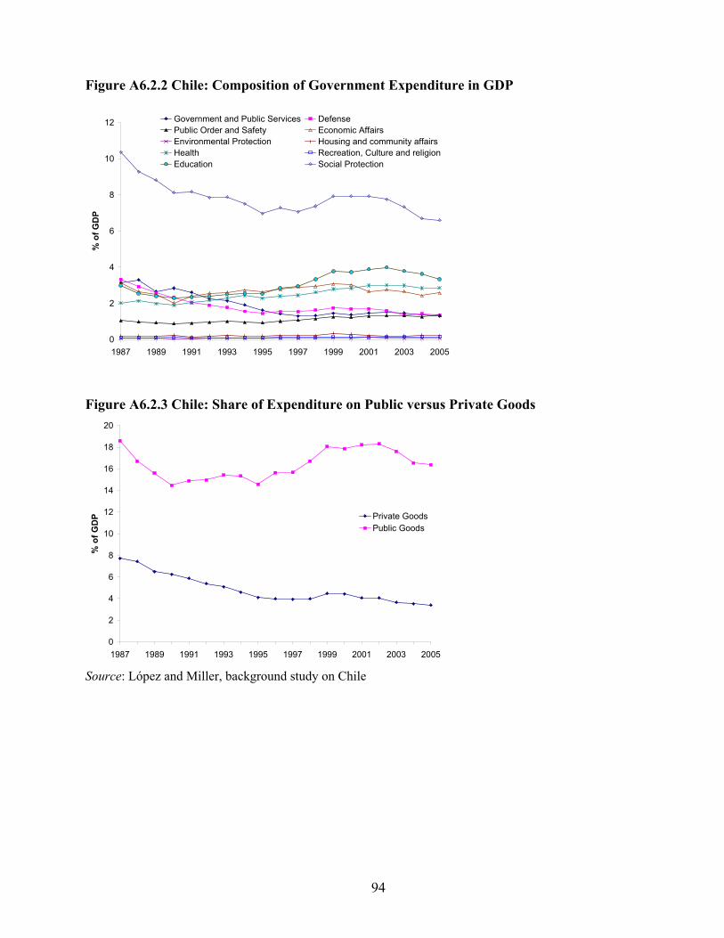
94
Figure A6.2.2 Chile: Composition of Government Expenditure in GDP
0
2
4
6
8
10
12
1987 1989 1991 1993 1995 1997 1999 2001 2003 2005
% o
f GD
P
Government and Public Services DefensePublic Order and Safety Economic AffairsEnvironmental Protection Housing and community affairsHealth Recreation, Culture and religionEducation Social Protection
Figure A6.2.3 Chile: Share of Expenditure on Public versus Private Goods
0
2
4
6
8
10
12
14
16
18
20
1987 1989 1991 1993 1995 1997 1999 2001 2003 2005
% o
f GD
P Private GoodsPublic Goods
Source: López and Miller, background study on Chile

95
Figure A6.2.4 Student Score in PISA Test 2000 and Cumulative Expenditure in Education
POL
ARG
PER
IDNBRA
MEX CHI
CZEHUN
GRC
KOR
IRL
ESP
PRT
DEU
GBRFIN
BEL
JPNCANAUS
SWE
FRA
ITA
NOR CHEDNK USA
AUT
300
350
400
450
500
550
600
0 10000 20000 30000 40000 50000 60000 70000 80000Cummualtive Expenditure per student at age 15 (using US converted PPP)
Average perforance (Reading, Mathematical and Scietific Literacy)
Source: OECD and United Nations Educational, Scientific, and Cultural Organization, 2003, Table 3.3. Table A6.2.2 Evolution of Poverty and Inequality (1987–2003) Year Poverty
(%) Extreme Poverty (%)
20/20 Index
10/40 Index Gini Coef
1987 45.1 17.4 .. .. 0.57 1990 38.6 12.9 14.0 3.5 0.58 1992 32.6 8.8 13.2 3.3 0.57 1994 27.5 7.6 14.3 3.5 0.57 1996 23.2 5.7 14.6 3.5 0.57 1998 21.7 5.6 15.5 3.5 0.58 2000 20.6 5.7 15.3 3.6 0.58 2003 18.8 4.7 14.3 3.3 0.57 Source: Mideplan, Social Division from CASEN Surveys

96
Table A.6.2.3 Income Distribution Before and After Simulated Tax Reform (with equal distribution of forgone taxes) Q5/Q1 10/40 D10/D1 10/(4+5+6) GINI Actual Indicators (2003) 14.3 13.4 34.1 7.3 0.50 Reform with Equal Distribution 12.7 12.1 28.1 6.8 0.48 Reform with Distribution Same as Monetary Subsidies 11.0 11.3 21.2 6.7 0.47 VAT Reduction 12.5**
Source: Own estimations based on 2003 CASEN, SII (2006), and household savings rate obtained from Butelman and Gallego (2001). Note: All indicators are based on household income rather than personal income; therefore, the Gini coefficients reported here are lower than those reported earlier, which were person based. ** For this exercise, we use monetary income and quintile data only, since we do not have the savings rate at the decile level, to compare expenditures and savings. The “before” reform in this case yields a Q5/Q1 of only 12.7. The value-added tax (VAT) rate is, however, reduced from 19 to 11.5 percent. Table A.6.2.4 Private Mining Rents as % of GDP 1997–2002 (in millions of current US$ and % of GDP) 1997 1998 1999 2000 2001 2002
Sales 4,263 3,367 4,167 5,207 5,141 4820
Operating costs 2,235 2,279 2,741 2,907 2,896 2,856
Depreciation 1,290 1,093 848 566 698 597
Financial costs 86 181 235 309 305 579
Taxes due 306 99 134 167 117 86
Rents (net profits) 1636 808 1057 1824 1823 1299
Rents as % of GDP 2.0% 1.0% 1.4% 2.4% 2.6% 2.0% Average rent 1997–2002 1.9% Source: Soto (2004) and own calculations.
6.3 Rebalancing China’s Growth Summary of the Country Case Study24 After three decades of exceptionally rapid growth, the sustainability of growth in terms of environment, equity, and even GDP growth itself is being widely debated in China. Indeed, the “quality of growth” and the “efficiency of growth” are now more important than the speed of growth, although rapid growth remains a goal as well. China is thus not seeking faster growth, but is seeking more equitable and sustainable growth. This paper argues that more sustainable growth will require a “third transformation” of the economy, which relies more on services and less on industry, more on productivity growth and less on capital accumulation, and more on domestic demand and less on net
24 Based on a background paper prepared by Bert Hofman and Louis Kuijs.

97
exports. The paper shows that a limited set of policies in the macroeconomic as well as the fiscal sphere would help improve the quality of growth. China’s rapid growth and poverty reduction is attributable to gradual marketization, openness to trade and investment, structural change, and urbanization. Productivity growth increased in the 1980s and early 1990s, which can be ascribed to reforms that followed the logic of learning and innovation very well: beginning with the homegrown institutional reforms in agriculture, followed by an expansion of township and village enterprises, gradual liberalization of prices, and opening up to the global economy. Gradual liberalization promoted a private-sector boom and competition, which allowed for gradual privatization. The more complex reforms started relatively late: fiscal reforms (1994) and financial reforms (after 2000). “Crossing the river by feeling the stones at the bottom” became the hallmark of China’s economic reform; implementing partial reforms in an experimental manner, often in a few regions; and expanding them upon proven success. This gradual reform also explains the relatively constant and even contribution of total factor productivity (TFP) to growth over the reform period. There are, however, some signs that the “easy” TFP growth that came along with marketization, opening up, and ownership reforms is now exhausted, and that without change future TFP is set to decline. Indeed, in the recent decade, China’s growth relied more heavily on physical capital accumulation rather than human capital accumulation, labor reallocation, and productivity growth. China’s current economic growth mode is not sustainable. The current growth pattern relies heavily on manufacturing industry and external demand, and requires ever-increasing capital accumulation. On current trends, investment in GDP would have to rise to more than 50 percent by 2020 and more than 55 percent by 2030 to achieve anticipated growth. As a result, the welfare that China gets out of this growth is less than optimal, and the question is whether the already low consumption share in the economy is politically sustainable. The export-oriented pro-growth policies and the accompanying large and growing current account surpluses have become an issue in the international arena, whereas domestically, the accumulation of international reserves is not only a macroeconomic issue, it also signifies a suboptimal allocation of resources. Growing Inequality. The current growth pattern has led to growing inequality. Accumulation of capital in urban industry has starkly widened productivity differences between urban and rural areas, which in turn have led to large income inequalities. China’s agriculture value added per capita in 2002 was about one-third of GDP per capita, whereas the same number for Indonesia was 0.65. China, with an estimated Gini coefficient of more than 0.45, is now less equal than the United States and Russia, and in current trends would be more like Latin American countries in terms of income inequality. The sharp rise in China’s inequality is partly caused by the country’s rapid transformation, partly as a result of the country’s development strategy and fiscal policies that yielded only limited redistribution through the budget: China’s coastal development strategy increased interprovincial inequalities, where preferential tax policies have benefited the coastal regions and the rich segment of the population. Meanwhile, the country’s household registration system hampered rural citizens in competing for higher-paid urban jobs. Farmers were taxed until recently when agricultural taxes were phased out, in 2004–6. As a result, agricultural incomes increasingly lagged average income per capita, contributing to income inequality. More recently, intraurban and intrarural inequality has been on the rise as well. Environmental Sustainability. The current growth pattern puts increasing strains on the environment. Although China has dramatically improved the efficiency of natural resources and energy use over the

98
past 30 years, environmental constraints on growth now loom large. A government report concluded that environmental degradation and pollution cost the Chinese economy the equivalent of 10 percent of GDP annually (SEPA 2006). This figure is corroborated by more specific costs reported in the Chinese press: up to $36 billion in lost industrial output from a lack of water to run factories, $13 billion from the degradation and health impact of acid rain, $6 billion from the spread of desert regions, and the list goes on.
The energy intensity of current-dollar GDP is on aggregate some four to six times that of advanced countries if measured in market exchange rates and prices; at an industry level, the energy intensity per volume of output is still some 1.5 to 2 times higher than in advanced economies.
The IEA predicts China’s greenhouse gas emissions could surpass those of the United States by 2009 or 2010 and double those of the world’s richest countries combined within 25 years.
China has 16 out of the 20-most-air-polluted cities in the world, and according to the State Environmental Protection Agency (SEPA), two-thirds of the urban population breathes air of substandard quality.
Water is becoming increasingly scarce relative to the nation’s requirements: the country has only one-third of the world average in water availability, and at the same time, the efficiency of water usage is low.
Soil erosion: Overall, 40 percent of China’s land is affected by soil erosion. The Chinese desert—already one-quarter of its land—is expanding at a rate of 1,900 square miles per year and is now encroaching on Beijing.
The consequence of pollution on the population is severe. Particulate matter, SO2, nitrogen oxide, and other pollutants are, according to the World Health Organization (WHO), the cause of 250,000 premature deaths a year. An estimated 2.35 million people die prematurely as a result of contaminated drinking water, indoor and outdoor air pollution, and other environmental risks (WHO 2006).
These downsides are in large part a result of the particular capital-intensive, industry-led growth that China has seen. In turn, China’s capital-intensive, industry-led growth pattern is largely a result of policies. The government has subsidized and favored industry and investment over the services sector and domestic consumption in several ways: (i) policies have encouraged saving and investment, with government spending been geared to investment in physical infrastructure instead of current spending on health and education; (ii) investment in industry has been encouraged in other ways as well, including via easy access to credit for large, industrial firms; (iii) industrialization has also been promoted by keeping the prices of inputs low; (iv) the reluctance to let the exchange rate appreciate in line with the reduction in unit labor costs in manufacturing has further stimulated the production of tradables; (v) prioritization of industry has also meant that the service sector did not get a lot of attention; and (vi) the containment of migration into urban areas has shaped the capital intensive nature of growth. The roles of fiscal policy and subsidies. China’s fiscal system is still in the process of transition from the planning model of “financing industrialization” to the market model of providing public goods and services.
The overall fiscal stance has improved since the Tax Sharing System reform of 1994, with the overall fiscal envelop reaching nearly 25 percent of GDP if one includes extrabudgetary funds and social security.

99
China has one of the most decentralized fiscal systems in the world. Fiscal disparities among subnational governments are larger in China than in most Organisation for Economic Co-operation and Development (OECD) countries: the richest province has more than eight times the per capita spending than the poorest provinces. The richest county has about 48 times the level of per capita spending than the poorest county (World Bank 2006).
While faced with vast regional disparities and rising income inequality, the fiscal system does too little to redistribute fiscal revenues across regions. The general equalization grant has been growing in recent years, but still makes up only 10 percent of all transfers to the regions. The outcomes are regressive (World Bank 2003, Dollar and Hofman 2007).
Equally, fiscal policy provides little income redistribution, with revenues from the personal income tax less than 1 percent of GDP.
In the area of expenditure policy, several noteworthy features are evident from figure A6.3.2 (based on Hussain and Stern 2007).
The share of culture, education, and health expenditure rose steadily in the 1980s but declined in the mid-1990s. Public expenditure on education has been low, falling short of the international average of 4 percent of GDP. Far more striking is the very low budgetary expenditure on health, which accounts for just 2.8 to 3.0 percent of expenditure (0.5 to 0.7 percent of GDP). This level of spending is exceptionally low by international standards. This problem is compounded by its highly skewed distribution. According to the Ministry of Health, about 80 percent of medical facilities are in urban areas, where 40 percent of China’s population lives. Rural areas, where 60 percent of China’s population live, have just 20 percent of medical facilities (People’s Daily online, January 11, 2005).
The share of expenditure accounted for by administration rose sharply, partly because of the method of valuation of the cost of administration. Wages and salaries account for much of this cost. The widening wedge between government and nongovernment wages forced the government to raise wages and salaries several times for civil servants.
The share of expenditure going to subsidies, mostly on goods, rose sharply in the 1980s, as the government attempted to compensate for some of the price effects of the liberalization of agriculture and other markets. The increase was followed in the 1990s by an almost equally sharp decline.
The share of expenditure on pensions, social welfare, and relief was remarkably small, partly because social insurance, which covers about 20 percent of the labor force and cost the government 4.2 percent of GDP in 2004, is off-budget. Including this spending, total expenditure on pensions, social welfare, and relief came to 4.6 percent of GDP, a much smaller percentage than in developed market economies.
In the recent years, China’s budget spending has increasingly focused on the provision of public goods, at 48 percent of total expenditure in 2005. At the start of reforms, spending patterns still reflected the traditional integration of enterprises in the budget, and subsequently reforms of the overall economic system were cushioned by subsidies to state enterprises (in the 1990s). In recent years, the share of private goods financed from the budget has precipitously declined to less than 20 percent of total (see figure A6.3.3).

100
China’s system of subsidies is also undergoing a transition. Studies on the beneficiary incidence of China’s subsidy policy are scarce. Based on official data, the size of quantifiable subsidies has been declining over time, currently at 2 percent of GDP, which seems to compare to those of other large developing countries, but the composition of the subsidies differs. Category I subsidies—including price subsidies and support to the state enterprises—rose in nominal terms, but the share in GDP has declined dramatically from a peak of 8 percent of GDP in 1985 to 0.7 percent in 2005. Among Category II quantifiable subsidies reported by the government to the WTO, the nonpoor, e.g., exporters and foreign invested enterprises, have benefited for longer periods of time. (Background paper by Wang, Yan.) In recent years, the government has started to take actions to address the above issues in fiscal policy in an attempt to rebalance growth and to build a “harmonious society.”
Between 2001 and 2006, agricultural taxes have been completed eliminated, and an increasing amount of fiscal resources was allocated to support agriculture, rural infrastructure, rural education, and rural health insurance.
The intergovernmental transfer system has also been rapidly expanding, whereas the government’s budgetary contribution to the pension system has started to lower the implicit pension debt.
The government has also started using the tax system to steer economic development in a more sustainable direction by increasing resource taxes and by differentiating export tax rebates according to energy intensity of the product exported. For example, on June 19, China’s Ministry of Finance eliminated VAT refund for 553 types of exports that are “heavily resource intensive” and heavy in emission and pollution, and reduced the refund rate for 2,286 types of other export products.
China is reviewing and reforming its system of subsidies. The recent decision to unify the corporate income tax rates for domestic and foreign-invested companies will end the tax privileges for foreign direct investors, which lasted for over 25 years.
Outstanding challenges remain to find a more rational basis for redistributing fiscal resources through transfers, rationalizing, and better managing earmarked transfers; moving to a truly individual income tax; and making major shifts in taxation and spending programs to promote sustainable development.

101
Figure A6.3.1 Less Poverty, More Inequality
0
10
20
30
40
50
60
1981
1982
1983
1984
1985
1986
1987
1988
1989
1990
1991
1992
1993
1994
1995
1996
1997
1998
1999
2000
2001
Pove
rty h
eadc
ount
25
35
45
Gin
i coe
ffici
ent
Inequality
Poverty
Source: World Bank staff estimates. Figure A6.3.2 China: Composition of Government Expenditure in GDP, Official Data
China: Composition of public expenditures (as % of GDP)
0
1
2
3
4
5
6
7
8
9
1980
1981
1982
1983
1984
1985
1986
1987
1988
1989
1990
1991
1992
1993
1994
1995
1996
1997
1998
1999
2000
2001
2002
2003
2004
Year
Perc
ent
Capital constructionCulture, education, and healthPensions, social welfare and reliefAdministrationSubsidies and enterprise capital
Source: Hussain and Stern 2007 based on data from http://www.stats.gov.cn

102
Figure A6.3.3 China: Share of Expenditure on Public versus Private Goods (consolidated general government expenditure)
Figure 1: China: Trends of shares of various types of expenditures in total budget
0%
10%
20%
30%
40%
50%
60%
70%
1980
1981
1982
1983
1984
1985
1986
1987
1988
1989
1990
1991
1992
1993
1994
1995
1996
1997
1998
1999
2000
2001
2002
2003
2004
2005
Year
Perc
ent
Share of public goods expenditures in totalgovernment expendituresShare of private goods expenditures in totalgovernment expendituresShare of administrative expenditures in totalgovernment expenditures
Source: Consolidated Government Expenditure. Computed using consistent analytical taxonomy with Chapter 2 based on data from the China and Mongolia Department of the World Bank
Source: Consolidated general government expenditures from China Country Management Unit of the World Bank. Data on debt interest, armed police troops, foreign affairs, and operating expenses of tax department were not included throughout. The sudden change in 1984–6 was related to the start of the state-owned enterprise reform and retrenchment, and that in 1999/2000 was largely the result of fiscal expansionary policy after the Asian financial crises.

103
Table A6.3.1 Comparative Structure of Aggregate Redistribution in China and Some OECD Countries (Percentage of GDP)
Germany Sweden USA Japan China
1994 2002
Factor income paid to households 77.4 74.5 80.1 75.6 56.6
- Employee compensation 54.8 58.6 59.8 56.3 51.9
Social contributions 20.4 16.9 8.6 9.5 2.9
- Employers 10.5 15.7 4.8 4.9 n.a.
- Others 9.9 1.2 3.8 4.7 n.a.
Social security payments 16.0 20.8 8.5 10.9 2.9
Direct taxes on household income 9.8 18.7 10.2 6.8 1
- Income tax 9.6 - 10.0 6.5
Noncontributory public transfers 4.4 5.9 3.9 1.1 2.1
Disposable income 67.5 65.5 73.7 71.2 56.9 Memo items: Other taxes 14.6 17.4 11.4 11.6 16.4
- of which indirect taxes 13.4 14.9 8.5 7.9 14.8 Overall tax rate (including social security contributions) 43.3 51.3 30.4 28.1 20.3 Taxes net of noncontributory transfers (available for government consumption and investment) 18.6 28.5 17.9 17.5 18.0 Source: National Accounts OECD, accessed through OECD and “Flow of Funds Accounts China 2002.” in NBS, China Statistical Yearbook 2006.
Source: Dollar and Hofman 2007, based on World Bank forthcoming. Note: Data for China are for 2003. Data for other countries are for various years. . .
Table A6.3.2 Share of Subnational Governments in Total Government
Developing Countries
OECD Countries
Transition Countries China
Subnational share of government tax revenues 9.27 19.13 16.59 40 Subnational share of government expenditure 13.78 32.41 26.12 73

104
6.4 India: More and Better Growth and the Role of Fiscal Policy Summary of Country Case Study25 Rapid growth since the 1980s has placed India among the top nine rapidly growing economies of the world, and in terms of total size, India rose from the world’s 50th economy in nominal U.S. dollars to the 12th largest in 2003. At the same time, questions have been raised about the quality of growth measured in terms of the distribution of the benefits of growth between income groups, especially the poor, and the impact on the natural environment. How effective have fiscal policies been in reconciling growth objectives with equity and environmental concerns? This paper first reviews the quality aspects of growth, including poverty, inequality, and the environment, and then focuses on the role of fiscal policy in achieving a more equitable and sustainable pattern of growth. Long-term growth. There are two distinct growth periods: the first phase from 1950 to 1980 was characterized by slow growth, with average GDP growing by only 3.6 percent per annum and by 1.2 percent in per capita terms. In the second phase from 1980 to 2004, growth accelerated to 5.7 percent on aggregate and to 3.8 percent in per capita terms. The service sector took off in the second phase, growing at 7.3 percent per year; the industrial sector maintained a steady growth of 6.3 percent; but agriculture lagged behind, growing at only 2.9 percent. Despite the rapid growth since 1980, India remains a low-income economy in per capita terms. For example, India’s per capita gross national product in 2005 was a mere 2 percent of that of the United States, suggesting that there is a huge amount of catching up still to be done. The quality aspects. In phase I, both rural and urban poverty increased even though income distribution improved, reflecting the stagnation of growth during this period. The pace of poverty reduction picked up substantially in phase II, and human development indicators were much improved. State-level analysis shows that poverty was reduced in all states and that there is a similar positive correlation between growth and poverty. So, it is reassuring that higher growth did allow India to make faster progress in improving the well-being of its citizens. Nevertheless, there is also evidence that income inequality increased in phase II and human development indicators remain weak by international standards, including the quality of health and education outcomes. Income inequality increased in urban areas, with the Gini coefficient rising from 0.34 in 1983/4 to 0.38 in 2004/5. These facts suggest that along with more rapid growth India needs to pay stronger attention to improving equity. One particular problem is the low employment elasticity of growth. India’s growth has been services-led and skill intensive, which reflects partly the policy bias in India’s past education policies in favor of higher and scientific education as opposed to basic education and training, and partly the effect of labor market controls that reduce employment flexibility and discriminate against labor-intensive enterprises. There are indeed pressing issues of low employment generation, and widening wage differentials between sectors and gender, that need to be addressed quickly.
25 Based on a background paper prepared by Sadiq Ahmed.

105
In India’s decentralized political environment where policies, resources, and institutions differ substantially by states, growth patterns have varied significantly between states. Evidence suggests that the gap between rich and poor states has widened particularly rapidly since the 1990s. Rising regional inequalities and the emergence of lagging regions with large concentrations of poor are of considerable social and political concern and are a major reason for pessimism among critics about the long-term sustainability of India’s growth. Addressing this lagging regional problem and arresting the rising income inequality trend are clearly major political economy challenges for India moving forward. Growing population, rapid urbanization, and rapid economic growth have all taken a toll on India’s natural environment. These are reflected in air and water pollution, deforestation, land and watershed degradation, and depletion of nonrenewable natural resources. One economywide measure is the concept of “adjusted net savings.” The estimated loss of national savings from environmental degradation is 5.8 percent of GNP for India, as compared with only 1.4 percent for high-income countries. Using the concept of ecological footprint, the gap between ecological footprint and the carrying capacity shows a significant deficit. The deficit is growing over time, thereby illustrating the need to pay much stronger attention to environmental concerns. Following years of neglect, attention to environmental management gained strength after the 1984 Bhopal disaster. Since then, there has been significant progress in developing environmental regulations and standards; however, overall implementation has been uneven between cities and states. The role of fiscal policies. Evidence suggests that India’s fiscal policy could be much more effective in promoting growth and poverty reduction. A conscious role for fiscal policy as a key instrument for environmental management is also lacking. Since the 1970s, India has run fairly big fiscal deficits (average of 8 percent of GDP) with the aim of pushing up growth. Yet, over the longer term this has resulted in building a huge domestic public debt and large interest payment obligations. Thus in 2004 the debt-to-GDP ratio exceeded 80 percent and interest payment climbed to over 7 percent of GDP, which was larger than the total public investment. On the whole, large interest payments and wage increases have considerably constrained India's ability to spend resources on infrastructure and human development, thereby constraining growth. More recently, the debate about fiscal deficits being good for growth has been set aside and governments at both the federal and state levels have been taking measures to contain fiscal deficits. Substantial progress has been made in improving and modernizing the tax structure. The introduction of the VAT at the state level has been a particularly important landmark. Nevertheless, there is scope for raising tax revenues through better tax administration, especially at the state level. Importantly, the challenge of restructuring public spending to better support growth and poverty reduction remains to be fully addressed. The main challenges for expenditure management are to contain the adverse effects of growing debt servicing on fiscal space, manage the wage bill prudently, and reform the subsidies. Interest spending grew rapidly over the past 40 years and by 2000 it absorbed over one-quarter of total consolidated government spending. This has severely restricted the fiscal space for other public spending, especially investment. There has been some progress recently with fiscal tightening, and the share of interest in total spending fell to 22 percent in 2005. Yet, the interest burden remains high and continued fiscal adjustment will be necessary to bring down interest costs to a more manageable level, thereby freeing resources for public investment. The wage bill of the federal and state governments absorbs some 25 percent of total consolidated spending. While the total size of the government employee pool is not large, there are concerns about

106
the quality and effectiveness of the civil service. Two related issues are the wage awards and pension liabilities. A generous wage award, particularly by the Fifth Pay Commission in 1998, has been a major reason for the worsening of the fiscal position at the state level. Thus, wage bills of the consolidated government surged from 5.4 percent of GDP in 1997 to 7.0 percent of GDP in 2000. As state governments continue to adjust to the burden of this last Pay Commission award, care has to be taken to avoid new pressures from future awards. The government, at both federal and state levels, should also exert considerable caution in new recruitments while endeavoring to improve efficiency and effectiveness. Similarly, growing pension liabilities could create a major fiscal headache in the future unless actions are taken to manage the financial burden. For example, the pension cost at the federal level doubled between 1995 and 2000, reaching 1 percent of GDP in 2000. The pension liabilities have also expanded substantially at the state level, in some cases reaching 2 percent of the state domestic product, making this the third-largest spending item after wages and interest expenses. Among the reforms that could help contain the fiscal burden include introducing funded, defined contribution pension schemes; moving from final wages to lifetime average earnings as the basis for calculating pension benefits; and improved management of the pension fund to maximize return from the accumulated surplus. Each year India spends about 5 percent of GDP in financial subsidies, including food, fertilizer, petroleum products, and electricity. (Economic subsidies are even higher, estimated at 14 to 15 percent of GDP.) Much of the subsidies are aimed at helping the poor, but evidence suggests that the actual benefits are likely to have accrued more to the richer segments of the population. As far as financial subsidies are concerned, they reflect spending on four key areas: food, fertilizer, petroleum, and electricity. Financial subsidies for food, fertilizer, and petroleum are provided partly through the federal government budget and account for some 95 percent of the total budgetary subsidy. Subsidy on electricity is provided by state governments to farmers for pumping ground water. This is done by controlling electricity prices for farmers. The rate of subsidy varies considerably by state, ranging from 100 percent (free power) to 10 percent (in West Bengal). Additionally, incidence analysis shows the poor targeting of this massive subsidy. Recent studies of Karnataka, Andhra Pradesh, and Tamil Nadu found that large farmers received 10 or more times the level of subsidies received by marginal farmers. In Madhya Pradesh, Punjab, and Haryana, medium and large farmers accounted for over three-quarters of the electric-pump-irrigated areas. Similarly, incidence analysis of health and education spending also suggest the scope for substantial improvement in equity. Econometric evidence from the state-level data suggests that fiscal policy could indeed be used much more effectively for influencing growth outcomes and poverty reduction than has been done so far. The detailed model, specification, estimation technique, and data are explained in the paper. The results suggest first that the composition of spending does matter for growth and poverty reduction. Spending on public goods such as health, education, and infrastructure has a much larger positive effect on growth than other spending, which includes spending on private goods such as subsidies. Specifically, reallocation of fiscal expenditures to increase the share of spending on public goods could lead the per capita gross state domestic product (GSDP) growth rate to increase on average by up to 2.7 percentage points (table A6.4.1). Second, spending on social public goods including education and health has a significantly positive effect on poverty reduction, as does state GDP per capita, while inflation has a negative effect. Reallocation of funds to increase the share of social-public-goods expenditures could reduce on average the poverty head count index by up to 6.6 percentage points (table A6.4.2). These results are pretty robust and consistent with theory and findings from cross-country studies.

107
There are numerous examples of how use of fiscal policy has had an unintentional negative impact on the environment. The most disturbing effects have resulted from the government’s farm subsidy policy. For example, subsidy on fertilizer has contributed to groundwater contamination while also leading to nutrient imbalances in soil. Indeed, the government has recognized this problem and this awareness has been an important factor underlying the effort to phase out fertilizer subsidy. The subsidy on power has contributed to inefficient and excessive extraction of groundwater, particularly in areas where electricity is provided free of charge. Subsidy on food grain production through the MSP program, along with power and fertilizer subsidies, have contributed to excessive focus on crops that are water and fertilizer intensive, leading to related environmental damage. Yet another example is the combination of import tariff and domestic pricing policy that has not only supported the use of environmentally damaging coal as opposed to more environmentally friendly fuels, but also has biased choice in favor of low-grade, higher carbon-emitting coal against high-grade, low-carbon coal. On the expenditure side, public spending on clean water, sanitation, and slum upgrading has been a positive factor for poverty and also has contributed to a better environment. The progress on access to clean water supply is particularly encouraging. Yet, total spending on these activities is much below what is necessary and the resource availability is severely limited by the inadequacy of the fiscal space. The way forward. Moving forward, the effectiveness of fiscal policy in helping India have more and better growth can be significantly improved. Already, India is making progress in reducing the fiscal deficit at both the federal and state levels based on tax reforms, which is helping create fiscal space for additional spending on infrastructure and human development. This progress should be deepened with the aim of raising taxes by another 2 to 3 percent of GDP and improving the quality of public spending. Specifically, the following can be accomplished:
There is substantial scope to reprioritize public spending, away from untargeted subsidies, interest cost, and expensive salary increases and toward health, education, and infrastructure. More spending on rural infrastructure, such as power, water, and roads, can help improve farm and nonfarm rural incomes.
Public spending programs on health and education, if well designed and delivered, can be a powerful tool for supporting better income distribution. In addition to raising the level of public spending in these activities, major efforts are needed to improve the service delivery system, including stronger public-private partnership and the reform of the public sector.
The management of the environment is receiving greater attention now than before. Yet, a comprehensive strategy that includes a conscious role for fiscal policy as a key instrument for environmental management is lacking. This requires urgent attention. Tax, subsidy, pricing, and expenditure policies can all play a critical role in improving the protection of the environment.

108
Figure A6.4.1 India: Composition of Government Expenditure as Share of GDP (consolidated government, federal, and state)
India: Composition of government expenditure in GDP
0
2
4
6
8
10
12
14
16
1985
1986
1987
1988
1989
1990
1991
1992
1993
1994
1995
1996
1997
1998
1999
2000
2001
2002
2003
2004
2005
Year
Perc
ent
Other expenditure on generalservices (including defense butexcluding administrativeservices)/GDP
Other developmentalexpenditures/GDP
Education and healthexpenditures as % of GDP
Administrative services/GDP
Source: Consolidated general government expenditures. Computed using consistent analytical taxonomy with Chapter 2 based on data from the South Asian Department (SASPR) of the World Bank
Figure A6.4.2 India: Various Types of Expenditure: Public versus Private Goods (Consolidated government, federal, and state)
India: Share of expenditure on public vs private goods
0
5
10
15
20
25
30
35
40
45
1985
1986
1987
1988
1989
1990
1991
1992
1993
1994
1995
1996
1997
1998
1999
2000
2001
2002
2003
2004
2005
Year
Perc
ent
Public goods expenditures/Totalexpenditure & net lending
Private goods expenditures/Totalexpenditure & net lending
Other expenditure on generalservices (including defense butexcluding administrativeservices)/Total expenditure & netlending
Administrative services/Totalexpenditure & net lending
Source: Consolidated General Government Expenditures. Computed using consistent analytical taxonomy with Chapter 2 based on data from the South Asian Department (SASPR) of the World Bank

109
Table A6.4.1 Estimating the Growth Effects of Public Spending (dependent variable: log difference of GSDP per capita [5MV1])
IV IV-RE2
State public goods spending share - 5MV 0.4340*** 0.4340**[2.69] [2.19]
State expenditures over GSDP - 5MV -0.5946* -0.5946[1.95] [1.54]
State other spending share - 5MV 0.2123*** 0.2123**[2.72] [2.06]
Dummy landlocked (with 1 indicating coastal) 0.0659 0.0659[1.34] [1.13]
India trade to GDP ratio - 5MV 0.2493*** 0.2493**[2.74] [2.20]
Proxy of state (AP) investment to GSDP ratio3 - 5MV 0.0004*** 0.0004**[2.72] [2.15]
Proxy of state (BH) investment to GSDP ratio - 5MV 0.0004*** 0.0004***[3.10] [2.69]
Proxy of state (GJ) investment to GSDP ratio - 5MV 0.0003** 0.0003*[2.42] [1.91]
Proxy of state (HY) investment to GSDP ratio - 5MV 0.0002*** 0.0002***[3.34] [2.95]
Proxy of state (KN) investment to GSDP ratio - 5MV 0.0003*** 0.0003**[2.77] [2.20]
Proxy of state (KR) investment to GSDP ratio - 5MV 0.0002*** 0.0002**[2.80] [2.20]
Proxy of state (MP) investment to GSDP ratio - 5MV 0.0005*** 0.0005***[3.51] [3.08]
Proxy of state (MH) investment to GSDP ratio - 5MV 0.0006*** 0.0006**[2.58] [2.12]
Proxy of state (OR) investment to GSDP ratio - 5MV 0.0002** 0.0002*[2.28] [1.77]
Proxy of state (PJ) investment to GSDP ratio - 5MV 0.0003*** 0.0003***[3.67] [3.27]
Proxy of state (RJ) investment to GSDP ratio - 5MV 0.0004*** 0.0004***[3.49] [3.12]
Proxy of state (TN) investment to GSDP ratio - 5MV 0.0005*** 0.0005**[2.99] [2.55]
Proxy of state (UP) investment to GSDP ratio - 5MV 0.0008*** 0.0008***[3.50] [3.06]
Proxy of state (WB) investment to GSDP ratio - 5MV 0.0004*** 0.0004**[2.86] [2.28]
Constant -0.3431*** -0.3431**[3.20] [2.44]
Observations 173 173Number of states 14 14
Hansen/Sargan test 0.3637Minimum value of F-statistics of all first stage regressions 20.06
Hausman test 0.3005Absolute value of z statistics in brackets (robust for IV).* significant at 10%; ** significant at 5%; *** significant at 1%.
1. Five-year moving average. 2. IV-FE regression shows that the null that all fixed error components are zero cannot be rejected. 3. State dummy times national investment as % of GSDP.
Note: the differences of the coefficients between IV and IV-RE are only visible starting at the 7th decimals which are not shown in the table.
Instrumented: state public goods spending share-5MV, state other spending share-5MV, and state expenditures/GSDP-5MV.Excluded instruments: federal public goods spending share-5MV, federal other spending share-5MV, federal taxes/GDP-5MV, federal expenditures/GDP-5MV, initial state urban population as % of total population(1990), initial state literacy rate (1991), initial state access to safe water(1990), and initial state access to electricity(1990).

110
Table A6.4.2 Instrumental Variables Estimation of Poverty Reduction Effects of Public Goods Spending Shares (dependent variable: head count poverty index [percentage points, under the national poverty line1])
IV IV-RE (Social)
IV-RE (Non-social)
IV-RE (Public goods)
Social expenditures, share in state expenditures2 -105.149** -81.214*
[2.55] [1.67]Non-social expenditures, share in state expednitures3 44.527
[1.14]Public goods expenditures, share in state expenditures4 -21.504
[0.40]State agriculture GDP as % of total state GDP -0.279 -0.353 -0.318 -0.176
[0.85] [0.97] [0.85] [0.53]Log of state GDP per capita -13.257** -9.451** -8.050* -11.654**
[2.18] [2.22] [1.66] [2.53]India inflation rate (consumer prices) 0.665 0.754*** 0.901*** 0.890***
[1.41] [2.69] [3.39] [3.48]Constant 188.463*** 150.819*** 107.522** 153.288***
[2.68] [3.44] [2.16] [2.59][1.14]
Observations 72 72 72 72Number of states 12 12 12 12Hansen-Sargan test 0.6139Minimum value of F-statistics of all first stage regressions 7.13Hausman test 0.5037 0.6330 0.9459Absolute value of z statistics in brackets (robust z statistics for IV)* significant at 10%; ** significant at 5%; *** significant at 1%
1. National poverty line=Rs. 49 per capita per month at Oct 73-June 74 rural prices
Instrumented: state agriculture GDP as % of total state GDP and shares of social, non-social and total Excluded instruments: Log of initial literacy rate (1991) and time dummies
2. Social public goods expenditures here are defined as state spending on education, sports, art and culture and on medical and public health and family welfare.3. Non-social public goods expenditures here are defined as state spending on rural development, irrigation and flood control, transport and communication, and power (capital expenditures only).4. Public goods expenditures is the sum of spending on education, sports, art and culture, medical and public health and family welfare, transport and communications, power (capital expenditures only), irrigation and flood control, and rural development.

111
6.5 Twelve Fast-Growing African Countries Summery of Country Case Study26 The sustained income growth during 1990-2005 in 12 reforming, low-income, nonoil countries has brought about a renewed optimism about the growth prospects of the Africa region. The fast-growing countries are Benin, Burkina Faso, Ethiopia, Ghana, Kenya, Madagascar, Malawi, Mali, Mozambique, Senegal, Tanzania, and Uganda. This section takes a deeper look into these fast-growing African economies to assess the quality aspect of the growth, and to evaluate whether government expenditures and policies might make the growth more pro-poor, equitable, and sustainable. Our analysis focuses on i) growth-poverty-inequality trends, ii) public spending patterns and beneficiary incidence analysis, and iii) public spending and the political economy.
Even though the 12 fast-growing countries had an average growth of about 4.1 percent per year for the past 15 years, as a group, these fast-growing African countries trail other developing countries in per capita income growth in large part because of higher population growth and slower productivity improvements. Aggregate total factor productivity grew by only 0.41 percent per year on average during the 1990s in these economies. It appears that economic reforms, in addition to economic recovery from a low economic base, have played an important role in postconflict countries. The effective use of large aid flows since the early 1990s, including the debt relief of the mid-1990s related to the Heavily Indebted Poor Countries Initiative, has contributed in part to the growth process in several of these countries. Quality aspects of growth. The recent growth seems to be associated with differential rates of poverty reduction and changes in inequality. Poverty was reduced in Burkina Faso, Senegal, Ghana, and Kenya during different periods, while it was actually increased in Madagascar in the past few years. A simple correlation analysis shows that growth is positively associated with poverty reduction in these countries, but it is also positively associated with income inequality. In particular, inequality has worsened significantly in Uganda, which is in part the result of the slow pace of growth in agriculture, and in part the result of inadequate job generation in other sectors. In fact, the fastest-growing sector in most African countries is the informal sector, which now accounts for over 40 percent of formal-sector GDP in each of the countries. There is a strong negative association between regulatory quality and the size of the informal sector, indicating that burdensome regulations combined with inadequate public infrastructure services could be driving small firms into the shadows. There is a positive association between real GDP growth and human development indicators. Underlying data indicates that, on average, growth is associated with increases in primary and secondary completion rates, and with narrowing of the gender gap in enrollment. Under-five mortality is estimated to have decreased by an average of about 18 percent during 1990–2005 for the sample. There exists, however, a negative but weak relationship between environmental sustainability (both green and brown indices) and real GDP growth. Even though air pollution is not a big issue, land degradation appears to have become the most important factor hampering agricultural productivity in Ghana, Uganda, Ethiopia, and Mali.
26 Based on a background paper prepared by by Raj Nallari.

112
Fiscal policy. Government revenue as a proportion of GDP has remained flat for decades in each of our selected countries. Revenue levels remain low at about 10 to 14 percent of GDP despite several attempts to strengthen tax administration systems in these sample countries. Revenue collection in other low-income countries is around 20 percent of GDP, while in developed countries as a whole it is in the range of 30 to 40 percent of GDP. This low revenue collection is constraining the governments’ developmental role in improving the quality of life. Fiscal resources increased after the Heavily Indebted Poor Countries Initiative was implemented, and since the mid-1990s, public spending on essential services of education, health, water, and sanitation rose significantly. The richer quintiles, however, appear to be benefiting disproportionately from public spending and service delivery, including subsidies on fuel (table A6.5.1). Uganda. Since the economic recovery around 1988/9, the real GDP growth averaged about 6.3 percent per year during 1990–2005. The growth-poverty and inequality pattern varied unevenly across the years. The first period of 1992–7 was characterized by high growth coinciding with significant poverty reduction (10.7 percent) and declining income inequality. This was followed by accelerated pro-poor growth during 1997–2000, which was accompanied by rising income inequality as the Gini coefficient rose from 0.35 to 0.40. The third period of 2000–3, however, featured slower average growth rate and rising inequality, leading to negative rates of pro-poor growth. About 0.7 percent of consumption accrued mainly to the top quintile, which was the only segment of population to benefit from the increase. The poverty head count rose from 34 percent to 38 percent of the population, and the Gini index continued to worsen, from 0.40 to 0.43. The use of public-expenditure tracking surveys and local media in identifying and minimizing leakages of public resources to local service-delivering units has had a significant positive impact on improving development effectiveness. Ghana. After trade liberalization and exchange-rate adjustment in 1991, Ghana has experienced impressive trade expansion (as exports increased from 33 percent in 1991 to over 81 percent by 1998), and real GDP growth averaged about 4.5 percent per year during 1990–2005. The reduction in poverty was very impressive, with the poverty head count reduced from 51.7 percent to 28.5 percent, which appears to be in line with achieving the goal of “halving the poverty incidence” (Coulombe and Wodon 2007). The better-off households benefited relatively more in growth, however, than the poorer segments of the population. As a result, income inequality rose since 1991, and the gap between the northern part and the rest of the country has widened. Poverty remains a rural phenomenon, but agricultural growth has lagged, and uncertainty in land tenure and ownership appears to be a major impediment. Poverty reduction occurred because of household decisions to move from less-advantaged areas or rural-agricultural activities to more advantaged areas or activities. Public spending in Ghana increased in infrastructure construction and related services, but funding for agriculture was reduced from 8 percent of GDP in the early 1990s to about 1 percent by 2003. The poorest groups obtained some benefit from public spending on education, but the richer quintiles received a larger share than the poorer quintiles, and also use these facilities more frequently. In education, public spending remains skewed toward the nonpoor, and very little has changed over the past 15 years. Health care spending reflects a similar bias toward more affluent groups. Ghana receives a significant amount of remittances, but richer households living in urban areas receive most of the international remittances, which are used for consumption and payment for education. Unfortunately, the poor quality of fiscal data prevented a deeper analysis of public spending in these countries. Political Economy. What explains these outcomes—limited private investment, low revenue collection, the rise in informal employment and output, and the inequitable growth pattern? There is a

113
long tradition of political economic analysis of African economic performance, and a few are discussed below.
• “Syndrome-free” nature of these economies (Fosu and O’Connell 2006) is one of the main reasons for higher growth in these 12 countries. All the countries have moved away from heavy reliance on controls and regulations, adverse redistributive schemes, unsustainable spending booms, and avoided state breakdown (e.g., Uganda under Idi Amin from 1971–86) during the last two decades and this has contributed to growth.
• Growth benefits are not shared equitably since countries in the tropics have tended to produce
“exploitative regimes” that protect the interest of a small elite. Particularly in countries where restraining institutions are absent, the government is likely to be captured by a small group (Acemoglu 2005, Easterly and Levine 1997 and 2003, and Alesina and Ferrara 2005). In addition to this, these 12 countries appear to be “weak economic states” as validated by governance indicators, such as government effectiveness, control of corruption, and regulatory quality (Kauffman et al 2006). Weak economic states lack capacity to tax, regulate, and play a development role. Self-interested elites will only invest if future private rewards are attractive, and in weak African states the elites prefer capturing rents now because they are uncertain about the state’s capacity to favor them in the future (Acemoglu 2005).
• “State capture” could be defined as the efforts of affluent elites to shape the laws, public policies,
and rules and regulations of the state to their advantage. The dynamics of state capture are complex, and it could be understood based on country-specific analysis of winners and losers not only in terms of income but also in terms of powerful groups and vested interests. There is some evidence from Uganda and Ghana that collusion between political elites and indigenous African, Asian, and Lebanese business groups (supported by bureaucracy) has ensured rent seeking, limited the pace of reforms, and restricted the entry of foreign capital and creation of jobs in the formal sectors.
Uganda is a good case in point where public access to information, expenditure tracking, and other measures are found to be a powerful deterrent to local “state capture.” In the early 1990s, although 20 percent of public education spending was directed to primary education, only 13 percent of the intended grants were reaching the end users and schools. The provision of mass information in local newspapers about the transfer of public funds for primary schooling enabled Uganda to significantly reduce district-level capture of public funds by local elites. Poor people benefited from such a transparency in allocation of public resources. In sum, poverty seems to be an outcome of complex relationships and economic and political arrangements. The argument of state capture by a small group of elites appears to hold in the 12-country sample, although further investigation is needed. A “highly captured” country, in the absence of effective institutions, is likely to suffer from low tax collection, lower public and private investment, and lower level of provision of public services to the poor. Firms that cannot compete with favored firms or accommodated groups will go under or have to resort to “informality.” In addition, land tenure and ownership uncertainties have limited agricultural growth and job creation. In a number of sample countries, the affluent groups benefited disproportionately from education, health, infrastructure, and subsidies. Evidence shows that the incidence of education and health spending becomes more pro-poor if there is a significant improvement in voice, accountability, and

114
governance. Much remains to be done for higher and better growth, particularly through structural reforms, in encouraging competition within the domestic economy and from abroad, improving land tenure and ownership, improving accessibility to infrastructure and social services, improving transparency, and minimizing leakage of subsidies to the nonpoor. Only sustained pressure from domestic advocacy groups, local media, and the international community could limit the collusion between political and business elites and the bureaucracy in Africa to implement reforms and move from rent seeking and redistribution to higher and shared growth. Figure A6.5.1 Empowerment Correlates with Lower Capture of Subsidies by the Elites
Source: Nallari, background study on 12 African countries.
Voice & Acct contain disparity in educ spending
0.0
1.0
2.0
3.0
4.0
5.0
6.0
0 10 20 30 40 50 60 70
voice and acct ranking (1-100)
prop
of e
duc
subs
idie
s to
top
20%
vs
botto
m 2
0%
Madagascar
y = -4.8152x + 2.4125R2 = 0.6385
-10.0 -8.0 -6.0 -4.0 -2.0 0.0 2.0 4.0 6.0
0.0 0.2 0.4 0.6 0.8 1.0 1.2 1.4 1.6 1.8 2.0
Annual GDP per capita growth (%)
Burkina Faso
B Ghana Senegal
Malawi A
nnual change in head count poverty (%)
Figure A6.5.2 Economic Growth and Poverty Reduction

115
Table A6.5.1 Beneficiary Incidence of Fuel Subsidies Share of Fuel Subsidies
Received by Bottom 40%
Share of Fuel Subsidies Received by Top 20%
Gabon 2005 (3.2% of GDP used)
18 48.3
Kenya 15.3 Ghana 23 Mali 23.9 Memo item: Kerosene 70–80% of subsidies
accrues to top 40–50% Source: Nallari, background paper on 12 African countries. Table A6.5.2 Gross and Net TFP Relative to China, 2000–04 Gross TFP Net TFP Ethiopia 0.50 0.25 Kenya 0.70 0.35 Mozambique 0.30 0.25 Senegal 0.80 0.65 Tanzania 0.65 0.40 Source: Benn Eifert, Alan Gelb, and Vijaya Ramachandran (2006) Business Environment and Comparative Advantage in Africa, p. 213, Annual Bank Conference on Development Economics, World Bank, Washington, DC, 2006.
Figure A6.5.3 Growth and Inequality
y = 0.4758x - 0.7451
R2 = 0.2582
-2 -1.5
-1 -0.5
0 0.5
1 1.5
2 2.5
0 0.5 1 1.5 2 2.5 3 3.5 4
Annual growth in per capita income (%)
Burkina
Ghana
Senegal
Madagasca
Uganda
Malawi
Annual change in inequality
(%)

116
Table A6.5.3 Agriculture Sector Indicators of 12 Fast-Growing African Countries, 1990–2005
Country Name
Share of women in agriculture labor force (%) 2003–05
Value added of agriculture(%) 1990–2005
Cereal Yield—average annual % growth 1990–2005
Rural population access to an all-season road (%) 1997–2004
Rural household access to electricity (%) 1995–2003
Average annual deforestation (%) 1990–2005
Benin 46.2 5.5 1.8 32.0 5.5 0.0 Burkina Faso 46.9 3.6 2.1 34.0 0.2 0.3 Ethiopia 40.0 2.4 0.9 32.0 0.4 0.3 Ghana 44.0 3.8 1.5 61.0 20.9 1.7 Kenya 49.0 2.6 -0.1 44.0 4.3 0.3 Madagascar 49.6 1.9 0.8 41.6 2.1 0.4 Malawi 56.0 6.2 2.5 38.0 1.4 0.8 Mali 46.0 2.9 3.5 n.a. 2.2 0.7 Mozambique 59.5 5.2 1.1 n.a. 2.1 0.2 Senegal 48.9 2.7 2.0 n.a. 6.0 0.5 Tanzania 46.3 1.8 1.9 n.a. n.a. 1.0 Uganda 49.2 3.9 1.9 n.a. 2.4 1.8 12 fast growing 48.47 3.54 1.66 34.43 4.32 0.67 Source: World Bank, 2007b. World Development Report on Agriculture for Development.

117
List of Background Papers For Sections 2–5 López, Ramón E., 2007. “More and Better Growth: Conceptual Framework and the Central Hypotheses.” A background note for “More and Better Growth” project. López, Ramón E., and Greg Galinato. 2007. “Should Governments Stop Subsidies to Private Goods? Evidence from Rural Latin America,” Journal of Public Economics 91 (5–6): 1071–94. López, Ramón E., and Asif Islam. “Fiscal Policy and the Environment.” Background note 3 for “More and Better Growth” project. López, Ramón E., and Sebastian Miller. “The Structure of Public Expenditure: A Robust Predictor of Economic Development?” Background paper 1 for “More and Better Growth” project. López, Ramón E., and Máximo Torero. “How Growth and Fiscal Policies Affect Income Distribution in Developing Countries.” Background paper 2 for “More and Better Growth” project. Flanagan, Ann Elizabeth. “Project Analysis.” Background note for “More and Better Growth” project. Country Studies Ahmed, Sadiq. “More and Better Growth in India: Role of Fiscal Policy.” Background paper for “More and Better Growth” project. Hofman, Bert, and Louis Kuijs. “Rebalancing China’s Growth.” Background paper for “More and Better Growth” project. López, Ramón E., and Sebastian J. Millar. “Chile and the Quality of Growth: Two Countries in One.” Background paper for “More and Better Growth” project. Nallari, Raj. “More and Better Growth in Twelve Fast-Growing African Countries.” Background paper for “More and Better Growth” project. Romano, Claudia, and Sergio Sakurai. “Quality of Growth, Government Expenditures and Tax Revenues in Brazil: 1990–2005” Background paper for “More and Better Growth” project. Wang, Yan. “China’s Subsidies: An Analysis on the Types and Quantity of Subsidies.” Background note for “More and Better Growth” project.

118
References Acemoglu, Daron. 2005. “The Persistence of Inefficient States,” draft available at www.mit.edu. Agénor, Pierre Richard, and Kyriakos C. Neanidis. 2006. “The Allocation of Public Expenditure and Economic
Growth.” Centre for Growth and Business Cycle Research Discussion Paper Series, University of Manchester, No. 69.
Aghion, Philippe, and Peter Howitt. 1998. Endogenous Growth Theory, Cambridge, MA: MIT Press. Alesina, Alberto, and Dani Rodrik. 1994. “Distributive Politics and Economic Growth.” Quarterly Journal of
Economics 109 (3): 465–90. Alesina, Alberto, Nouriel Roubini, and Gerald D. Cohen. 1997. Political Cycles and the Macroeconomy.
Cambridge, MA: MIT Press. Alessina, Alberto, and La Ferrara, Eliana; (2001). “Preferences for Redistribution in the land of Opportunities”.
NBER Working Paper No. 8267. Cambridge, MA. National Bureau of Economic Research. ———.. 2005. “Ethnic Diversity and Economic Performance,” Journal of Economic Literature, vol 63
(September) pp 762-800 Allcott, Hunt, Daniel Lederman, and Ramon López. 2006. “Political Institutions, Inequality, and Agricultural
Growth: The Public Expenditure Connection.” Policy Research Working Paper Series 3902, World Bank, Washington, DC.
Anderson, Kym, Will Martin, and Ernesto Valenzuela. 2006. “The Relative Importance of Global Agricultural
Subsidies and Market Access.” World Trade Review 5 (3): 357–76. Arbache, Jorge, Delfin S. Go, and John Page. 2008. “Is Africa’s Economy at a Turning Point?” Policy Research
Working Paper 4519. The World Bank. Arjona , Roman, Ladaique, Maxime and Pearson, Mark; (2003). Growth, Inequality and Social Protection.
Canadian Public Policy / Analyse de Politiques, Vol. 29, Supplement: The Linkages between Economic Growth and Inequality (Jan., 2003), pp. S119-S139
Aschauer, David. 1989. “Is Government Spending Productive?” Journal of Monetary Economics 23: 177–200. Asian Development Bank (ADB). 2006. “Government Financial Statistics” The ADB publication. Manila. Atkinson, Anthony B. 2003. “Income Inequality in OECD Countries: Data and Explanations.” CESifo Working
Paper Series 881, Munich. Baig, Taimur, Amine Mati, David Coady, and Joseph Ntamatungiro. 2007. “Domestic Petroleum Product Prices
and Subsidies: Recent Developments and Reform Strategies.” IMF Working Paper WP/07/71. Barro, Robert J. 1990. “Government Spending in a Simple Model of Endogenous Growth.” Journal of Political
Economy 98 (5): S103–26. ———. 1991. “Economic Growth in a Cross Section of Countries.” The Quarterly Journal of Economics 56
(425): 407–43.
119
Barro, Robert J., and Jong-Wha Lee. 2001. “International Data on Educational Attainment: Updates and Implications.” Oxford Economic Papers 53 (3): 541–63.
Bassett, William, F. John P. Burkett, and Louis Putterman. (1999). “Income Distribution, Government
Transfers, and the Problem of Unequal Influence. European Journal of Political Economy”, 15(2), June, pp. 207-228.
Baydas, Mayada, Richard Meyer, and Nelson Aguilera-Alfred. 1994. “Credit Rationing in Small-Scale
Enterprises: Special Microenterprise Programmes in Ecuador.” Journal of Development Economics, 31: 279–309.
Benabou, Roland, (1996). Inequality and Growth. NBER Macroeconomics Annual 1996, edited by Ben S.
Bernanke and Julio Rotemberg. Cambridge MA: MIT Press. ———. (2000). “Unequal Societies: Income Distribution and the Social Contract”. American Economic
Review, 90(1), March, pp. 96-129. Bernauer, Thomas, and Vally Koubi. 2006. “States as Providers of Public Goods: How Does Government Size
Affect Environmental Quality?” Available at Social Science Research Network: http://ssrn.com/abstract=900487 (accessed May 2006).
Bernauer, Thomas and Patrick Kuhn. 2006. “Does Trade Promote Effective International Environmental
Problem Solving?” University of Zurich CIS Working Paper No. 13. Available at SSRN: http://ssrn.com/abstract=900486 (accessed May 2006).
Bertola, G., 1993. Factor shares and savings in endogenous growth. American Economic Review 83(5).1184–
1198. Besley, Timothy, and Robin Burgess, 2004. “Can Labor Regulation Hinder Economic Performance? Evidence
from India.” Quarterly Journal of Economics 119 (1) (February): 91–134. Bird, Richard M., and Barbara Diane Miller. 1989. “The Incidence of Indirect Taxes on Low-Income
Households in Jamaica.” Economic Development and Cultural Change 37 (2):393–409. Bourguignon, Francois. 2005. “The Dynamics of Institutions, Development and Elites.” Speech at the Annual
Bank Conference on Development Economics 2005; also published in Beyond Transition 16 (4) (October–December):19-21.
Bourguignon, Francois, and Pereira da Silva Luiz. 2003. The Impact of Economic Policies on Poverty and
Income Distribution. Washington, DC: Oxford Press and World Bank. Bourguignon, Francois, and Christian Morrisson. 1998. “Inequality and Development: The Role of Dualism.”
Journal of Development Economics 57: 233–57. Bradley, David, Evelyne Huber, Stephanie Moller, Francoise Nielsen, and John Stephens; (2001). “Distribution
and Redistribution in Post Industrial Democracies”. Luxembourg Income Study. Working Paper No. 265. Syracuse, NY: Center for Policy Research, Syracuse University, May.
Buchanan, James M. 1950. “Federalism and Fiscal Equity.” In The Economics of Fiscal Federalism and Local
Finance, 1998, pp. 347–63. Edited by Wallace E. Oates, Edward Elgar Publishing Limited, Cheltenham UK.

120
Calmon, Paulo. 2004. “Evaluation of Subsidies in Brazil: An Overview.” Working paper sponsored by a World Bank research grant.
Cashin, Paul. 1995. “Government Spending, Taxes, and Economic Growth.” IMF Staff Papers 42 (2): 237–69. Castello, Amparo and Domenech, Rafael; (2002). “Human Capital Inequality and Economic Growth: some new
Evidence”. The Economic Journal 112, March, pp. C187-C200. Chomitz, Kenneth G. 2007. At Loggerheads? Agricultural Expansion, Poverty Reduction, and Environment in
the Tropical Forest. A World Bank Policy Research Report. World Bank Publication, Washington, DC.
Chong, Alberto, and Mark Gradstein. 2004. “Inequality and Institutions.” Research and Development Working
Paper No. 506. Inter-American Development Bank, New York, NY. Coady, David. 2006. “Indirect Tax and Public Pricing Reform.” In Analyzing the Distributional Impacts of
Reform, ed. Aline Coudouel and Stefano Peternostro. Washington, DC: World Bank. Coady, David, Moataz El Said, Robert Gillingham, Kangni Kpoda, Paulo Medas, and David Newhouse. 2006.
“The Magnitude and Distribution of Fuel Subsidies: Evidence from Bolivia, Ghana, Jordan, Mali, and Sri Lanka,” IMF Working Paper 06/247, Washington, DC.
Coulombe, Harold and Quentin Wodon. 2007. “Poverty, Livelihood, and Access to Basic Services in Ghana:
An Overview” April 2007 in Ghana Country Economic Memorandum: Meeting the Challenge of Accelerated and Shared Growth. World Bank.
Dasgupta, Partha. 1990. “Well-Being and the Extent of Its Realization in Developing Countries.” Economic
Journal 100 (4 [suppl.]). pp. 1-32.
———. 1996. “The Economics of the Environment.” Environment and Development Economics 1 (4): 387–428.
———. 2003. “Sustainable Economic Development in the World of Today’s Poor.” . In Scarcity and Growth in the New Millennium, ed. R. David Simpson, Michael A. Toman, and Robert U. Ayres. Resources for the Future Inc. Baltimore, MD: John Hopkins University Press (forthcoming).
Dasgupta, Partha, and Karl-Goran Maler. 1994. “Poverty, Institutions, and the Environmental Resource Base.”
Environment Paper, 64 (9). World Bank, Washington, DC. David, Paul A., Bronwyn H. Hall, and Andrew A. Toole. 2000. “Is Public R&D a Complement or Substitute for
Private R&D? A Review of the Econometric Evidence.” Research Policy 29 (4–5): 497–529. de Ferranti, David, Guillermo E. Perry, Daniel Lederman, and William Maloney. 2002, “From Natural
Resources to the Knowledge Economy—Trade and Job Quality.” World Bank Latin American and Caribbean Studies, Washington, DC.
de la Fuente, Angel. 1997. “Fiscal Policy and Growth in the OECD.” CEPR Discussion Paper No. 1755, Centre
for Economic Policy Research, London. de la Fuente, Angel., and Rafael Doménech. 2000. “Human Capital in Growth Regressions: How Much
Difference Does Data Quality Make?” OECD Economics Department Working Paper No. 262, Paris.

121
Deaton, Angus. 2003. Health, Inequality and Economic Development. Journal of Economic Literature, Volume
41, Number 1, 1 March 2003, pp. 113-158(46). ———. 2005, "Measuring Poverty in a Growing World (or Measuring Growth in a Poor World).” Review of
Economics and Statistics 87 (1) (February): 1–19. Deininger, Klaus, and Squire, Lyn; (1998). New Ways of Looking at Old Issues: Inequality and Growth.
Journal of Development Economics, Vol 57,pp. 257-287. Devarajan, Shantayanan, Vinaya Swaroop, and Heng-fu Zou. 1996. “The Composition of Public Expenditure
and Economic Growth.” Journal of Monetary Economics 37 (2–3): 313–44.
Diamond, Arthur M. 1999. “Does Federal Funding ‘Crowd In’ Private Funding of Science?” Contemporary Economic Policy 17 (4): 423–31.
Dollar, David, and Aart Kraay. 2002. “Growth is Good for Poor.” Journal of Economic Growth 7 (3): 195–225. ———. 2004. “Trade, Growth and Poverty.” Economic Journal (Royal Economic Society) 114 (493): f22–
f49,02.
Dollar, David, and Bert Hofman. 2007. “Intergovernmental Fiscal Reforms, Expenditure Assignment, and Governance.” In Public Finance in China: Reform and Growth for a Harmonious Society. Development Economics Research Group, World Bank, Washington, DC, December. Edited by Jiwei Lou and Shuilin Wang 39-52.
Easterly, William, Timothy Irwin, and Luis Serven. 2007. "Walking up the down escalator : public investment
and fiscal stability," Policy Research Working Paper Series 4158, The World Bank. Easterly, William, and Ross Levine. 1997. “Africa’s Growth Tragedy: Policies and Ethnic Divisions” Quarterly
Journal of Economics, vol 112 (4) pp. 1203-50. Easterly, William, and Sergio Rebelo. 1993. “Fiscal Policy and Economic Growth.” Journal of Monetary
Economics 32: 417–58. ECLAC (Economic Commission for Latin America). 2006. Social Panorama of Latin America 2005. New
York: United Nations Publications. Esteban, Joan, and Debraj Ray. 2006. “Inequality, Lobbying, and Resource Allocation.” American Economic
Review 23: 257–79. FAO-BID. 2006. “Crecimiento, inversión privada y eficiencia del gasto público en las áreas rurales de América
Latina y el Caribe.” In “Políticas Públicas Y Desarrollo Rural En América Latina Y El Caribe: El Papel Del Gasto Público”, edited by Fernando Soto Baquero, Józimo Santos Rocha, Jorge Ortega, Oficina Regional De La Fao Para América Latina Y El Caribe, Santiago, Chile. 127-164
Ferreira, Francisco and Michael Walton. 2005. “The Inequality Trap.” Finance and Development 42 (4): 34–7. Fine, Benjamin, and Fine Kit. 1974. “Social Choice and Individual Rankings, I and II,” Review of Economic
Studies, Vol. 41, No. 3. (Jul., 1974), pp. 303-322. and Vol. 41, No. 4. (Oct., 1974), pp. 459-475.

122
Fischer, Stanley. 1993. “The Role of Macroeconomic Factors in Growth.” Journal of Monetary Economics 32 (3):485–512.
Fosu, Augustin Kwasi and Stephen O’Connell. 2006. “Explaining African Economic Growth” in Growth and
Integration edited by F. Bourguignon and B. Pleskovic. Annual Bank Conference on Development Economics, Dakar, Senegal. World Bank, Washington DC.
Furman, Jason, Lawrence H. Summers, and Jason Bordoff. 2007. “Achieving Progressive Tax Reform in an
Increasingly Global Economy.” The Hamilton Project. Washington, DC: The Brookings Institution. June 2007.
Ghosh, Sugata, and Udayan Roy. 2004. “Fiscal Policy, Long-Run Growth, and Welfare in a Stock-Flow Model
of Public Goods.” Canadian Journal of Economics 37 (3): 742–56. Goetz, Stephan J., David L. Debertin, Angelos Pagoulatos. 1998. “Human Capital, Income, and Environmental
Quality: A State-Level Analysis.” Agricultural and Resource Economics Review 27 (2): 200–8. Goni, Edwin, Humberto J. Lopez, and Luis Serven. 2008. “Fiscal Redistribution and Income Inequality in Latin
America”. World Bank Policy Research Working Paper 4487. Goodman, Leo A., and Markowitz Harry 1952. “Social Welfare Functions Based on Individual Rankings.”
American Journal of Sociology 58 (3): 257–62. Granado, Javier Arze del, Cut Dian R.D. Agustina, Tim Bulman, Wolfgang Fengler and Mohamad Ikhsan.
2008. “Indonesia at $100 per Barrel: The impact of oil and gas prices on public finance.” Working paper at the World Bank Office Jakarta. Gray, Cheryl, Tracey Lane, and Aristomene Varoudakis, eds. 2007. Fiscal Policy and Economic Growth: Lessons for Eastern Europe and Central Asia. Washington, DC: World Bank.
Grier, Kevin B., and Gordon Tullock. 1989. “An Empirical Analysis of Cross-National Economic Growth
1950–1980.” Journal of Monetary Economics 24 (1): 259–76. Growth Commission. 2008. All papers will be available on the web. http://www.growthcommission.org
Guellec, Dominique, and Bruno van Pottelsberghe. 1999. “Does Government Support Stimulate Private R&D?”
OECD Economic Studies 29 (1997/II): 95–122. Guo, Jang-Ting and Kevin J. Lansing. 2002. “Fiscal Policy, Increasing Returns and Endogenous Fluctuations.”
Macroeconomic Dynamics 6 (5): 633–64. Gupta, Sanjeev, Hamid R. Davoodi, and Rosa Alonso-Terme. 1998. “Does Corruption Affect Income Inequality
and Poverty?” IMF Working Paper Series WP/98/76. International Monetary Fund, Washington, DC. Gylafson, Thorvaldur, and Zoega, Gylfi; (2003). “Education, Social Equality and Economic Growth: A View of
the Landscape” CESifo Working Paper Series No. 876. Center for Economic Studies and Institute for Economic Research.
Hamilton, Kirk. 2000. ‘Sustaining Economic Welfare: Estimating Changes in Per Capita Wealth.” World Bank
Policy Research Working Paper #2498. The World Bank, Washington, DC. Hanushek, Eric A., and Ludger Woessmann. 2007. “The Role of Education Quality for Economic Growth.”
World Bank Policy Research working paper, no. WPS 4122, Washington, DC.

123
Heitger, Bernhard. 2001. “The Scope of Government and Its Impact on Economic Growth in OECD Countries.”
Kiel Working Paper No. 1034, Kiel Institute for the World Economy, Germany. Helfand, Steven. 2001. ‘The Distribution of Subsidized Agricultural Credit in Brazil: Do Interest Groups
Matter?” Development and Change 32: 465–90. Heller, Peter S. 2005. “Understanding Fiscal Space”, IMF Policy Discussion Paper No. 05/4. Washington DC,
March 1, 2005. Herrera, Santiago. 2007. “Public Expenditure and Growth.” World Bank Policy Research Working Paper 4372,
Washington, DC. Herrera, Santiago, and Gaobo Pang. 2006. “Efficiency of Public Spending in Developing Countries: An
Efficiency Frontier Approach.” Policy Research Working Paper Series 3645, World Bank, Washington, DC.
Heston, Alan, Robert Summers, and Bettina Aten. 2006. Penn World Table Version 6.2. Center for International
Comparisons of Production, Income and Prices at the University of Pennsylvania, Philadelphia. Hoff, Karla, and Joseph Stiglitz. 2000. “Modern Economic Theory and Development.” In Frontiers of
Development Economics, ed. Meier, Gerald and Joseph Stiglitz. New York: Oxford University Press and the World Bank. pp.389-459.
Hussain, Athar, and Nicholas Stern. 2007. “Public Finances, the Role of the State, and Economic
Transformation, 1978–2020.” In In Public Finance in China: Reform and Growth for a Harmonious Society. Development Economics Research Group, World Bank, Washington, DC, December. Edited by Jiwei Lou and Shuilin Wang. pp.13-38.
IMF (International Monetary Fund), , 2003. “Fiscal Adjustment in IMF-Supported Programs.” Independent
Evaluation Office. Washington, DC:IMF. ———. 2006. Government Financial Statistics. CD-ROM. Washington, DC: International Monetary Fund. ———. 2008. “The Fiscal Implications of Climate Change”, Fiscal Affairs Department, Washington DC, Feb
22, 2008. Imrohoroglu, Ayse, Antonio Merlo, and Peter Rupert. 2000. “On the Political Economy of Income
Redistribution and Crime.” International Economic Review 41 (1): 1–25. Isham, Jonathan, and Daniel Kaufmann. 1995. “The Forgotten Rationale for Policy Reform: The Productivity of
Investment Projects.” Policy Research Working Paper 1549, and later published in the Quarterly Journal of Economics 114 (1): 149–84.
Isham, Johnathan, Daniel Kaufmann, and Lant H. Pritchett. 1997. “Civil Liberties, Democracy, and the
Performance of Government Projects.” World Bank Economic Review 11(2) (May): 219–42. Islam, Nazrul. 1995. “Growth Empirics: A Panel Data Approach.” Quarterly Journal of Economics,110: 1127–
70. Jones, Larry E., Rodolfo E. Manuelli, and Peter E. Rossi. 1993. “Optimal Taxation in Models of Endogenous
Growth.” Journal of Political Economy 101 (3): 485–517.

124
Kamps, Christophe. 2004. “New Estimates of Government Net Capital Stocks for 22 OECD Countries 1960–
2001.” IMF Working Paper 04/67, International Monetary Fund, Washington, DC. Kaufmann, Daniel, and Yan Wang. 1995. “Macroeconnomic Policies and Project Performance in the Social
Sectors: A Model of Human Capital Production and Evidence from LDCs.” World Development 23 (5): 751–65.
Keefer, Philip, and Stuti Khemani. 2003. "The Political Economy of Public Expenditures.” World Bank
Working Paper 26953, Washington, DC. ———. 2005. “Democracy, Public Expenditures, and the Poor: Understanding Political Incentives for
Providing Public Services." World Bank Research Observer 20 (1):1–27. Keefer, Philip, and Stephen Knack. 2007. “Boondoggles, Rent-Seeking, and Political Checks and Balances:
Public Investment under Unaccountable Governments.” Review of Economics and Statistics 89 (3): 566-72.
Kenworthy, Lane and Pontusson, Jonas; (2002). “Inequality and Redistribution in OECD countries”. Ithaca
NW, Cornell University, Mimeo. King, Robert and Ross Levine. 1993. “Financial Intermediation and Economic Development.” In Financial
Intermediation in the Construction of Europe, ed. Colin Mayer and Xavier Vives, 156–89.. London: Centre for Economic Policy Research.
Kneller, Richard. Michael F. Bleaney, and Norman Gemmell. 1999. “Fiscal Policy and Growth: Evidence from
OECD Countries.” Journal of Public Economics 74 (2): 171–90. Kochhar, Kalpana, Utsav Kumar, Raghuram Rajan, Arvind Subramanian, and Ioannis Tokatlidis. 2006. “India’s
Pattern of Development: What Happened, What Follows.” Journal of Monetary Economics, 53 (5) (July): 981–1019.
Kristov, Lorenzo, Peter Linder, and Rober McClelland; (1992). “Pressure Groups and Redistribution”. Journal
of Public Economics 48(2), 135-163. Krugman, Paul. 1994. “The Myth of Asia’s Miracle.” Foreign Affairs 73(6):. 62–78. Lecocq, Franck, and Zmarak Shalizi. 2007. “How Might Climate Change Affect Economic Growth in
Developing Countries: A Review of the Growth Literature with a Climate Lens.” World Bank Policy Research Working Paper 4315, August, Washington, DC.
Lee, Young, and Roger H. Gordon. 2005. “Tax Structure and Economic Growth.” Journal of Public Economics
89 (5–6): 1027–43. Levine, Ross, and David Renelt. 1992. “A Sensitivity Analysis of Cross-Country Growth Regression.”
American Economic Review 82 (4): 942–63. Li, Hongyi, Lyn Squire and Heng-fu Zou. 1998. “Explaining International and Intertemporal Variations in
Income Inequality.” Economic Journal 108 (446): 26-43.

125
Lindert, Kathy, Emmanuel Skoufias, and Joseph Shapiro. 2006. “Redistributing Income to the Poor and the Rich: Public Transfers in Latin America and the Caribbean.” World Bank SP Discussion Paper no. 605, Washington, DC.
Litchfield, Julie A., Phillippe G. Leite, and Francisco Ferreira. 2006. “The Rise and Fall of Brazilian Inequality,
1981–2004.” The World Bank, Policy Research Working Paper Series 3867, Washington, DC. Lledo, Victor, Aaron Schneider, and Mick Moore. 2004. “Governance, Taxes, and Tax Reform in Latin
America.” IDS Working Paper 221. Institute of Development Studies, University of Sussex, UK. Loayza, Norman V, and Claudio Raddatz. 2006. “The Composition of Growth Matters for Poverty Alleviation.”
World Bank Policy Research Working Paper no. WPS 4077, Washington, DC. Lopez, Humberto, and Luis Serven. 2006. “A Normal Relationship? Poverty, Growth, and Inequality.” World
Bank Policy Research Working Paper no. WPS 3814, Washington, DC. López, Ramón. 2003. “The Policy Roots of Socioeconomic Stagnation and Environmental Implosion: Latin
America 1950–2000”. World Development 31 (2): 259–80. ———. 2005. “Why Government Should Stop Non-Social Subsidies: Measuring their Consequences for Rural
Latin America.” World Bank Policy Research Working Paper 3609, Washington, DC.
———. 2007. “Market Failure, Government Subsidies and Aggregate Investment.” Unpublished manuscript, University of Maryland, College Park.
López, Ramón. and Greg Galinato. 2007. “Should Governments Stop Subsidies to Private Goods? Evidence
from Rural Latin America.” Journal of Public Economics 91 (5–6): 1071–94.
Loury, Glen. 1981. “Intergenerational Transfers and the Distribution of Earnings,” Econometrica 49 (4) (July): 843–67.
Lundberg, Mattias and Lyn Squire. 2003. “The Simultaneous Evolution of Growth and Inequality.” The
Economic Journal 113: 326–44. Mankiw, N. Gregory, David Romer, and David N. Weil. 1992. “A Contribution to the Empirics of Economic
Growth.” Quarterly Journal of Economics 107: 407–37. Mati, Amine 2008. “Developments in Domestic Fuel Prices, Taxes and Subsidies in Selected Countries”, Fiscal
Affairs Department, the IMF, Washington DC. Mauro, Paolo. 1998. “Corruption and the Composition of Public Expenditure.” Journal of Public Economics 69:
263–79. Milanovic, Branko. 2000. “The Median Voter Hypothesis, Income Inequality, and Income Distribution: An
Empirical Test with the Required Data.” European Journal of Political Economy 16(3): 367–410. Milesi-Ferretti, Gian Maria., Roberto Perotti, and Massimo Rostagno. 2002. “Electoral Systems and Public
Spending.” Quarterly Journal of Economics 117 (2): 609–57.

126
Moene, Karl O, and Wallerstein, Michael; (2001). “Inequality, Social Insurance and Redistribution”. American Political Science Review, 95(4), 859-874.
National Bureau of Statistics (NBS). China Statistical Yearbook 2006. China Statistical Press, Beijing. Nourzad, Farrokh, and Martin Vrieze. 1995. “Public Capital Formation and Productivity Growth: Some
International Evidence.” Journal of Productivity Analysis 6 (4): 283–95. Oates, Wallace E. 1999. “An Essay on Fiscal Federalism.” Journal of Economic Literature 37 (3) (September):
1120–49. Odedokun, Matthew and Jeffery Round.. 2004. “Determinants of Income Inequality and Its Effects on
Economic Growth: Evidence from African Countries.” Revue Africaine de Developpement (African Development Review) 16 (2): 287–327.
OECD (Organisation for Economic Co-operation and Development). Environmental Indicators, p. 104. See also
Myriam Linster and Frederique Zegel, “Pollution Abatement and Control in OECD Countries.” 2007 OECD Working Group on Environmental Information and Outlooks, ENV/EPOC/SE(2007)1 at www.oecd.org via.
OED (Operations Evaluation Department). Country Assistance Evaluations for China (2005) , Brazil (2004),
and India (2001). World Bank, Washington, DC. ———. 2005. 2004 Annual Review of Development Effectiveness: The World Bank’s Contribution to Poverty
Reduction. Washington, DC: The World Bank Publication. Osberg, Lars S; (1995). “The Equity/Efficiency Tradeoff in Retrospect”. Canadian Business Economics, 3(3),
pp. 5-20. Padovano, Fabio, and Emma Galli. 2001. “Tax Rates and Economic Growth in the OECD Countries (1950–
1990).” Economic Inquiry 39 (1): 44–57. ———. 2002. “Comparing the Growth Effects of Marginal vs. Average Tax Rates and Progressivity.”
European Journal of Political Economy 18 (30): 529–44. Pang, Gaobo, Brian Pinto, and Marina Wes. 2007. “India Rising—Faster Growth, Lower Indebtedness.” Policy
Research Working Paper 4241, The World Bank, Washington, DC. June. Patrinos, Harry Anthony, Cris Ridao-Cano, and Chris Sakellariou. 2006. "Estimating the Returns to Education:
Accounting for Heterogeneity in Ability.” World Bank Policy Research Working Paper no. WPS 4040, World Bank, Washington, DC.
Perotti, Roberto. 1992. “Income Distribution, Policies, and Growth”. American Economic Review 82(2),
pp.311-316. ———. 1996. “Growth, Income Distribution, and Democracy. What the Data Say”. Journal of Economic
Growth, 1(2), 149-316 ———. 2007. "Fiscal Policy in Developing Countries: A Framework and Some Questions.” World Bank Policy
Research Working Paper no. WPS 4365, World Bank, Washington, DC.
127
Persson, Torsten, and Tabellini, Guido; (1994). “Is Inequality Harmful for Growth?”. American Economic Review, 84(3), pp. 600-621.
Piketty, Thomas. “Income Inequality in France, 1901–1998.; (2003). ” Journal of Political Economy, 2003,
111(5), pp. 1004–42.
Piketty, Thomas, and Saez, Emmanuel.; 2003.“Income Inequality in the United States, 1913–1998.” Quarterly Journal of Economics, 2003, 118(1), pp. 1–39.
Piketty, Thomas, and Saez, Emmanuel. 2006. “The Evolution of Top Incomes: A Historical and International
Perspective” AER, Papers and Proceeding, Vol. 96. No.2 pp. 200-205. Pinto, Brian, and Farah Zahir. 2004. “India: Why Fiscal Adjustment Now?” Policy Research Working Paper
3230, World Bank, Washington, DC. March. Pritchett, Lant.1996. “Mind Your P’s and Q’s: The Cost of Public Investment Is Not the Value of Public
Capital.” World Bank, Policy Research Working Paper Series no. WPS 16600, World Bank, Washington, DC.
Psacharopoulos, George, and Harry Anthony Patinos. 2002. “Returns to Investment in Education: A Further
Update.” World Bank Policy Research Working Paper #2881, World Bank, Washington, DC. Ravallion, Martin. 1998. “Does the Aggregation Hide the Harmful Effects of Inequality on Growth?”
Economics Letters 61 (1998): 73–7. ———. 2001. “Growth, Inequality and Poverty: Looking Beyond Averages.” World Development, 29 (11):
1803–15. ———. 2004. “Pro-Poor Growth: A Primer.” The World Bank Policy Research Working Paper no. 3242,
World Bank, Washington, DC. ———. 2005. “A Poverty-Inequality Trade-off?” Journal of Economic Inequality 3 (2) (August): 169–81. ———. 2007, “Geographic Inequity in a Decentralized Anti-Poverty Program: A Case Study of China.” World
Bank Policy Research Working Paper no. WPS 4303, World Bank, Washington, DC. Ravallion, Martin, and Shaohua Chen, 2004. “China's (Uneven) Progress Against Poverty.” World Bank Policy
Research Working Paper no. WPS 3408, World Bank, Washington, DC. Ravallion, Martin, Mark T. Heil, and Jyotsna Jalan. 2000. “Carbon Emission and Income Inequality.” Oxford
Economic Papers 52 (4) (October): 651-669. Reinikka, Ritva and Jakob Svensson. 2004. “Local Capture: Evidence from a Central Government Transfer
Program in Uganda” in The Quarterly Journal of Economics, vol 119, no. 2, pages 679-705 Resnick, Danielle, and Regina Birner. 2006. “Does Good Governance Contribute to Pro-Poor Growth? A
Review of the Evidence from Cross-Country Studies.” DSGD Discussion Paper No. 30. International Food Policy Research Institute, Washington, DC.
Romer, Paul. 1990. “Endogenous Technological Change.” Journal of Political Economy. 98 (5): S71–102.

128
Ross, Catherine, and Wu, Chia-ling; (1995). “The links between Education and health”. American Sociological Review, Vol. 60, No. 5 (Oct., 1995), pp.719-745.
Rothschild, Michael and Joseph Stiglitz. 1976. “Equilibrium in Competitive Insurance Markets: An Essay on the Economics of Imperfect Information.” Quarterly Journal of Economics 90 (4): 630–49.
Saez, Emmanuel and Veall, Michael R; (2005). “The Evolution of High Incomes in Northern America: Lessons from Canadian Evidence.” American Economic Review, 2005, 95(3), pp. 831–49.
Sala-i-Martin, Xavier. 1997a. “I Just Ran Two Million Regressions.” American Economic Review 87 (2): 178–
83. ———. 1997b. “Transfers, Social Safety Nets, and Economic Growth”. IMF Staff Papers, 44(1), pp. 81-102. Sanchez-Robles, Blanca. 1998. “Infrastructure Investment and Growth: Some Empirical Evidence.”
Contemporary Economic Policy 16 (1): 98–108. Schwatz, Gerd, and Teresa Ter-Minassian. 2000. “The Distributional Effects of Public Expenditure.” Journal of
Economic Surveys 14(3) (July): 337–58. SEPA (State Environmental Protection Agency). 2006. Environmental Forecast and Countermeasure in China
of the Year 2005. Beijing: Qinghua University Publishing. Serven, Luis. 2007. “Fiscal Rules, Public Investment, and Growth”. World Bank Policy Research Working
Paper 4382. Shadbegian, Ronald.J., and Wayne B. Gray. 2003. “What Determines Environmental Performance at Paper
Mills? The Roles of Abatement Spending, Regulation, and Efficiency.” Center for Economic Studies, U.S. Census Bureau, Working Papers. Washington, DC.
Shalizi, Zmarak. 2007. “Energy and Emission: Local and Global Effects of the Rise of China and India.” World
Bank Policy Research Working Paper 4209. April. World Bank, Washington, DC. SII (Servicio de Impuestos Internos). 2005. “Ley contra la evasion tributaria: Compromisos y cumplimientos en
el ambito de la administracion tributaria interna.” Subdirección de Estudios SII. Santiago, Chile. ———.2006. Informe de gasto tributario. Subdirección de Estudios SII. Santiago, Chile. Smith, John H. 1973. “Aggregation of Preferences with Variable Electorate.” Econometrica 41: 1027–42. Smith, V. K. 1995. “Social Benefits of Education: Feedback Effects and Environmental Resources.” Duke
University, Department of Economics, Working Papers 95-14. Duke University, Durham, NC. Soto, Raimundo, 2004. “Capital Subsidies and the Quality of Investment in Chile.” Working Paper sponsored
by a World Bank research grant. World Bank, Washington, DC.
Stern, Nicholas H. 1984. “Optimum Taxation and Tax Policy.” IMF Staff Papers 31 (June): 339–78. ———.2006. The Economics of Climate Change: The Stern Review. London: United Kingdom
Treasury/Cabinet Office.

129
Stiglitz, Joseph, and Andrew Weiss. 1981. “Credit Rationing in Markets with Imperfect Information.” American Economic Review, 71 (3): 393–410.
Tanzi, Vito, and Howell H. Zee. 1997. “Fiscal Policy and Long-run Growth.” IMF Staff Papers 44 (June): 179–
209. Ter-Minassian, Teresa, and Annalisa Fedelino. 2007. “Fiscal Policy and Reforms: Toward Realizing a
Harmonious Society.” In China’s Public Finance and Harmonious Society World Bank Development Economics Research Group. Washington, DC.
Thomas, Vinod. 2006. From Inside Brazil-Development in a Land of Contrasts. Washington, DC: World Bank.
Palo Alto, CA: Stanford University Press. Thomas, Vinod, and Yan Wang. 1996. “Distortions, Interventions, and Productivity Growth: Is East Asia
Different?” Economic Development and Cultural Change v. 44, iss. 2, pp. 265-88. Thomas, Vinod., Mansoor Dailami, Ashok Dhareshwar, Ramon E. López, Daniel Kaufmann, Nalin Kishor, and
Yan Wang. 2000. The Quality of Growth. New York: Oxford University Press.
Thomas, Vinod, Yan Wang, and Xibo Fan. 2003. “Measuring Education Inequality: Gini Coefficients of Education.” World Bank Policy Research Working Papers 2525, World Bank, and later published in Journal of Education Planning and Administration,17 (1): (January 2003): 5–33.
Turnbull, Geoffrey K. and Djoundourian, Salpie S; (2005). The median voter hypothesis: Evidence from general purpose local governments. Public Choice, Vol. 81, No. 3-4, pp. 223-240.
Uchida, Emi, Scott Rozelle, and Jintao Xu. 2007. “Conservation Payments, Liquidity Constraints and Off-Farm
Labor: Impact of the Grain for Green Program on Rural Households in China.” Forthcoming. United Nations Environment Program. 2007. “CEO-4 Environment for Development.” Global Environment
Outlook. V. 4. Van der Ploeg, Frederick; (2003). “Do Social Policies Harm Employment and Economic Growth?” CESifo
Working Paper Series No. 886. Center for Economic Studies and Institute for Economic Research, European University Institute.
Wang, Yan. 2006. “Inequality in Education in China and the World.” Published in ed. Shuanglin Lin, Beijing:
Peking University Press. Wang, Yan, and Yudong Yao. 2003. “Sources of China’s Economic Growth 1952–1999: Incorporating Human
Capital Accumulation.” China Economic Review 14 (2003): 32–52. Webb, Steven B. 2004a. “Bargaining for a new fiscal pact in Mexico.”, World Bank Policy Research Working
Paper 3284. ———. 2004b. “Fiscal Responsibility Laws for subnational discipline: the Latin American experience.” World
Bank Policy Research Working Paper 3309. White, Howard, and Edward Anderson. 2001. “Growth versus Distribution: Does the Pattern of Growth Pattern
of Growth Matter?” Development Policy Review 19 (3): 267–89.
130
Widmalm, Frida. 2001. “Tax Structure and Growth: Are Some Taxes Better Than Others?” Public Choice 107 (3–4): 199–219.
Wikstrom, Magnus (1999). “Income Distribution Effects from Local Public Expenditures in the Swedish
Municipalities”, Department of Economics University of Umea. Mimeo. Wong, Christine W. and Deepak Bhattasali. 2003. China: National Development and Sub-National Finance.
Beijing: CITIC Press. World Bank. 2001. World Development Report: The Challenge of Development. New York: Oxford University
Press. ———. 2003a. World Development Report: Sustainable Development. New York: Oxford University Press. ———. 2003b. Inequality in Latin America and the Caribbean. Washington, DC: World Bank Publication. ———. 2003c. China: Country Economic Memorandum: Growth with Equity. Washington, DC: World Bank
Publication. ———. 2005a. Pro-poor Growth in the 1990s: Lessons and Insights from 14 Countries. Operationalizing
Pro-poor Growth Research Program. Washington, DC: World Bank. ———. 2005b. Economic Growth in the 1990s: Learning from a Decade of Reform. Washington, DC: World
Bank. ———. 2006a. Equity and Development. World Development Report. New York: Oxford University Press. ———. 2006b. Where is the Wealth of Nations? Measuring Capital for the 21st Century, Washington, DC:
World Bank. ———. 2006c. Annual Review of Development Effectiveness 2006: Getting Results. Independent Evaluation
Group. Washington, DC: World Bank Publication. ———. 2006d. “The Challenges of African Growth” by Benno Ndulu and others, World Bank, Washington
DC. ———. 2006e. “Growth and Integration” edited by F. Bourguignon and B. Pleskovic. Annual Bank
Conference on Development Economics, Dakar, Senegal. World Bank, Washington DC. ———. 2007a Annual Review of Development Effectiveness. Independent Evaluation Group. Washington,
DC: World Bank Publication. ———. 2007b. Development Results in Middle-Income Countries. An Evaluation of the World Bank’s
Support. Report no. 39962, June 8, 2007. Independent Evaluation Group. Washington, DC: World Bank.
———. 2007b. World Development Report 2008 on Agriculture. New York: Oxford University Press. ———. 2007c. International Trade and Climate Change: Economic, Legal, and Institutional Perspectives.
November 14, 2007. Washington, DC: World Bank.

131
———. 2007d. “Delivering On the Promise of Pro-Poor Growth”, edited by T. Belsey and L. Cord, Palgrave Macmillan and World Bank, Washington DC.
World Health Organization. 2006, Preventing Disease through Healthy Environments—Towards an Estimate of
the Environmental Burden of Disease. WHO Press, World Health Organization, Geneva, Switzerland Worthington, Andrew C. 2001. “An Empirical Survey of Frontier Efficiency Measurement Techniques in
Education,” Education Economics, 9 (3) (December): 245–68.
132
Endnotes 1 As shown by IEG’s recent reports; in particular, the Annual Review of Development Effectiveness (World Bank-IEG
2007a), and the Development Results in Middle Income Countries report (World Bank-IEG 2007b), and ongoing work. 2 Many other dimensions of quality can be considered, including the nature of health outcomes, level and variability of
nutrition, macroeconomic fluctuation and volatility of growth, prevalence of crime and violence, and so forth. We have focused on poverty and income distribution and environmental sustainability as overarching attributes which, in turn, are also reflections of other aspects of quality. Especially given the limitations of time and resources, such a restricted focus on quality indicators may be justified. For a broader analysis on growth, see forthcoming work by the Growth Commission, led by Professor Michael Spence, at http://www.growthcommission.org.
3 The macroeconomic impact of fiscal deficits, while crucially important to growth and investment climates, is not the focus of this study since it has been the topic of many cross-country analyses on growth. See, for example, Perotti 2007, Serven 2007, Easterly, Irwin and Serven 2007, Easterly and Rebelo 1993, Fischer 1993, and Levine and Renelt 1992, among others.
4 There are a few recent studies such as IMF 2008 using simulations but empirical work is rare. 5 The term public good is often used to refer to goods that are non-excludable and non-competitive. This means that it is not
possible to exclude individuals from the good's consumption, and that each individual's consumption of the good leads to no subtractions from any other individual's consumption of that good. Due to difficulties in defining property rights and in pricing them, public goods are subject to market failures, where a non-coordinated market tends to undersupply such a good. The term government spending on public goods is broadly defined to include spending on education, health, social security, transport, communication, public order and safety, and housing and community amenities.
6 Stern 2006. 7 See, for example, the Annual Review of Development Effectiveness (IEG 2007a) and the Development Results in Middle
Income Countries report (IEG 2007b). 8 Thomas et al. 2000. 9 See, for example, Ravallion and Chen 2004; Christiaensen, Demery, and Kuhl 2006; and Loayza and Raddatz 2005;
World Bank 2005. 10 Hofman and Kuijs (background paper on China). 11 Granado, Agustina, Bulman, Fengler and Ikhsan 2008 “Indonesia at $100 per barrel: the impact of oil and gas prices on
public finance.” Working paper and presentation, March 10, 2008. 12 IEG 2007a. 13 Hofman and Kuijs (background paper on China). 14 World Bank 2007b. 15 WHO 2006. 16 The adjusted net savings is obtained by first adjusting gross national savings, by allowing for depreciation of capital
stock and then adding back spending on education, and subtracting losses of national wealth from deforestation, energy depletion, mineral depletion, carbon dioxide damage, and particulate emission damage.
17 WHO 2006 . 18 Nallari (background paper 5) and annex 6.5. 19 See for example, Bourguignon 2003, Hoff and Stiglitz 2000, Ravallion 2004; Dasgupta, 1996, World Bank Pro-poor
Growth study 2005a, World Bank 2005b, World Bank WDR 2006a on equity, World Bank 2007b WDR on Agriculture, Coady 2006, Schwartz and Ter-Minassian 2000, Serven 2007, Lopez and Serven 2007, Gray, Lane and Varoudakis 2007, and Loayza and Raddatz 2006, and Perotti 2007. On the environment, see OECD, 1999, Bernauer and Koubi, 2006, Lecocq and Shalizi 2007, Webb 2004, The Stern Review 2006, IEG report on PRSP; and on-going IEG work on Public Sector Reform and Governance; on sustainable development, and on Climate Change, 2007.
20 Nallari (background paper on 12 African countries). 21 See background paper by López and Miller (background paper 1, and annex 3.1). 22 The data used in background paper 1 cover only the central government expenditures and excludes local governments. In
most countries, the central government spends a high portion of public expenditures. Moreover, in the few cases where we have data for central and local government expenditures, there is a high correlation between the public goods/private goods ratios or shares between local government expenditures and the central government expenditures (for example, in Brazil such correlation coefficient is about 0.82). Since the econometric findings use 5-year averages as basic data points, there is the question of the short time span in observing effects. While some of the investments in public goods are likely to have maturity periods of longer than 5 years (e.g., formal education), others such as expenditures in skill training, certain health improvements, agriculture technical extension, are likely to yield dividends much quicker. More important, a reallocation of expenditures involves reducing expenditures in private

133
goods which are likely to have negative productivity effects by inducing market distortions. Removing such expenditures is thus likely to have more rapid effects well within the five-year period. Finally, at least some of the econometric results rely as much in cross-country variance as within country variability, the former of which is likely to contain long-term information.
23 Three background papers, including López and Miller (2007). 24 López and Galinato 2007. 25 López and Galinato 2007. 26 Ahmed (Background paper on India) and annex 6.4. 27 Background paper 4 on project analysis using IEG data, by Flanagan. 28 Results are to be interpreted with caution. Good ratings on individual projects alone do not always translate to good
results at the sector or country level. For example, individual project success in increasing school enrollments may not mean better educational outcomes if they are not targeted and supported by sectorwide actions.
29 See background paper by López and Miller on Chile. 30 Hofman and Kuijs (background paper on China). 31 Yan Wang’s background note on subsidies in China. 32 See figure 1.4. 33 Background paper on Brazil (Romano and Sakurai )and annex 6.1. 34 Nallari [Background paper on 12 African countries]. 35 Chile SII 2006 36 See Dollar and Hofman 2007, and annex 6.3. 37 See annex 6.4 and background paper Ahmed [on India]. 38 Nallari [Background paper on 12 African countries]. 39 This has been shown in the literature; see for example, Bourguignon 2004a, 2004b; Lopez and Serven 2006; Deininger and
Squire, 1996; Chen and Ravallion, 1997, Ravallion 1998, 2004; World Bank 2006 [WDR on Equity and Development]. 40 On the second line of research looking into the link between inequality and the median voter’s desired pattern of policies,
see Deininger and Squire 1998, Persson and Tabellini 1994, Bertola 1993, Arjona et.al. 2003, Turnbull and Salpie S. Djoundourian 2005, Milanovic 2000, Bassett, et.al. 1999, Alessina and La Ferrara 2001, Kristov et.al. 1992; and for recent literature on this topic, Moene and Wallerstein (2001), Bradley et.al. (2001), and Kenworthy and Pontusson (2002). On the third branch of the literature focusing on inequality and growth, since they are both affected by redistributive public spending, particularly health and education spending, see Ross and Wu (1995), Perroti (1992, 1996), Bassett et.al. (1999), Pearson and Tabellini (1994), Alesina and Rodrik (1994), Osberg (1995), Sala-i-Matin (1997), Benabou (1996, 2000), Castello and Domenech (2002), and, most recently, van der Ploeg (2003), Gylafson and Zoega (2003), and Deaton (2003). Most of these studies conclude that there is no direct link between inequality and public spending in health and education.
41 See Wikstrom (1999) and recent work by Piketty and Saez (2006, 2003), Pickety (2003), and Saez and Veall (2005). 42 Background paper 2 by López and Torero. 43 Using data from 70 developing countries in the 1990s, Ravallion (2005) found no evidence of a tradeoff between absolute
poverty incidence and relative inequality. The main reason is that economic growth shows little correlation with changes in relative inequality. But there is evidence of a tradeoff for absolute inequality, suggesting that those who want to lower the absolute gap between the rich and poor must be willing to see lower absolute levels of living for poor people.
44 Background paper by Nallari. 45 Table A6.4.2 in the background paper by Ahmed and annex 6.4. 46 World Bank 2006b, p.177. 47 See Coady 2006 for a review. 48 See annex 6.2. 49 WHO 2006. 50 OECD 1999. 51 Bernauer and Koubi 2006. 52 Background paper by López and Islam . 53 This is a concern because PM10 is, by far, the most harmful pollutant to health. 54 Konisky 1999 . 55 Bernauer and Koubi 2006. 56 López and Galinato 2007. 57 López and Galinato 2007. 58 López and Galinato 2007.