The Project Gutenberg eBook #38993: The …The Project Gutenberg EBook of The Integration of...
86
The Project Gutenberg EBook of The Integration of Functions of a Single Variable, by G. H. Hardy This eBook is for the use of anyone anywhere at no cost and with almost no restrictions whatsoever. You may copy it, give it away or re-use it under the terms of the Project Gutenberg License included with this eBook or online at www.gutenberg.org Title: The Integration of Functions of a Single Variable Author: G. H. Hardy Editor: P. Hall F. Smithies Release Date: September 23, 2012 [EBook #38993] Language: English Character set encoding: ISO-8859-1 *** START OF THIS PROJECT GUTENBERG EBOOK INTEGRATION OF FUNCTIONS OF ONE VARIABLE ***
Transcript of The Project Gutenberg eBook #38993: The …The Project Gutenberg EBook of The Integration of...

The Project Gutenberg EBook of The Integration of Functions of a SingleVariable, by G. H. Hardy
This eBook is for the use of anyone anywhere at no cost and withalmost no restrictions whatsoever. You may copy it, give it away orre-use it under the terms of the Project Gutenberg License includedwith this eBook or online at www.gutenberg.org
Title: The Integration of Functions of a Single Variable
Author: G. H. Hardy
Editor: P. HallF. Smithies
Release Date: September 23, 2012 [EBook #38993]
Language: English
Character set encoding: ISO-8859-1
*** START OF THIS PROJECT GUTENBERG EBOOK INTEGRATION OF FUNCTIONS OF ONE VARIABLE ***
Produced by Brenda Lewis, Anna Hall and the OnlineDistributed Proofreading Team at http://www.pgdp.net (Thisfile was produced from images generously made availableby The Internet Archive/American Libraries.)
transcriber’s note
Minor typographical corrections and presentational changes have beenmade without comment.
This PDF file is optimized for screen viewing, but may easily be re-compiled for printing. Please see the preamble of the LATEX source file forinstructions.

Cambridge Tracts in Mathematicsand Mathematical Physics
General EditorsP. HALL, F.R.S. and F. SMITHIES, Ph.D.
No. 2
THEINTEGRATION OF FUNCTIONS
OF A SINGLE VARIABLEBY
G. H. HARDY
CAMBRIDGE UNIVERSITY PRESS

Cambridge Tracts in Mathematics
and Mathematical PhysicsGeneral Editors
P. HALL, F.R.S. and F. SMITHIES, Ph.D.
No. 2
The Integration of Functions of aSingle Variable

THE
INTEGRATION OF FUNCTIONSOF A SINGLE VARIABLE
BY
G. H. HARDY
SECOND EDITION
CAMBRIDGEAT THE UNIVERSITY PRESS
1966

PUBLISHED BYTHE SYNDICS OF THE CAMBRIDGE UNIVERSITY PRESS
Bentley House, 200 Euston Road, London, N.W. 1American Branch: 32 East 57th Street, New York, N.Y. 10022
First Edition 1905Second Edition 1916Reprinted 1928
19581966
First printed in Great Britain at the University Press, CambridgeReprinted by offset-litho by Jarrold & Sons Ltd., Norwich

PREFACE
This tract has been long out of print, and there is still some demand for it.I did not publish a second edition before, because I intended to incorporateits contents in a larger treatise on the subject which I had arranged to writein collaboration with Dr Bromwich. Four or five years have passed, and itseems very doubtful whether either of us will ever find the time to carryout our intention. I have therefore decided to republish the tract.
The new edition differs from the first in one important point only. Inthe first edition I reproduced a proof of Abel’s which Mr J. E. Littlewoodafterwards discovered to be invalid. The correction of this error has led meto rewrite a few sections (pp. 36–41 of the present edition) completely. Theproof which I give now is due to Mr H. T. J. Norton. I am also indebtedto Mr Norton, and to Mr S. Pollard, for many other criticisms of a lessimportant character.
G. H. H.
January 1916.

CONTENTS
page
I. Introduction 1
II. Elementary functions and their classification 3
III. The integration of elementary functions. Summary of results 8
IV. The integration of rational functions 11
1–3. The method of partial fractions 11
4. Hermite’s method of integration 15
5. Particular problems of integration 17
6. The limitations of the methods of integration 20
7. Conclusion 22
V. The integration of algebraical functions 22
1. Algebraical functions 22
2. Integration by rationalisation. Integrals associated with conics 23
3–6. The integral∫Rx,
√ax2 + 2bx+ c dx 25
7. Unicursal plane curves 32
8. Particular cases 35
9. Unicursal curves in space 37
10. Integrals of algebraical functions in general 38
11–14. The general form of the integral of an algebraical function.Integrals which are themselves algebraical 38
15. Discussion of a particular case 45
16. The transcendence of ex and log x 47
17. Laplace’s principle 48
18. The general form of the integral of an algebraical function (con-tinued). Integrals expressible by algebraical functions and log-arithms 48
19. Elliptic and pseudo-elliptic integrals. Binomial integrals 50
20. Curves of deficiency 1. The plane cubic 51
21. Degenerate Abelian integrals 53
22. The classification of elliptic integrals 54
VI. The integration of transcendental functions 55
1. Preliminary 55
2. The integral∫R(eax, ebx, . . . , ekx) dx 56
3. The integral∫P (x, eax, ebx, . . . ) dx 59
4. The integral∫exR(x) dx. The logarithm-integral 63
5. Liouville’s general theorem 63
6. The integral∫
log xR(x) dx 64
7. Conclusion 65
Appendix I. Bibliography 66
Appendix II. On Abel’s proof of the theorem of v., § 11 69

THE INTEGRATION OF FUNCTIONS
OF A SINGLE VARIABLE
I. Introduction
The problem considered in the following pages is what is sometimes calledthe problem of ‘indefinite integration’ or of ‘finding a function whose dif-ferential coefficient is a given function’. These descriptions are vague andin some ways misleading; and it is necessary to define our problem moreprecisely before we proceed further.
Let us suppose for the moment that f(x) is a real continuous functionof the real variable x. We wish to determine a function y whose differentialcoefficient is f(x), or to solve the equation
dy
dx= f(x). (1)
A little reflection shows that this problem may be analysed into a numberof parts.
We wish, first, to know whether such a function as y necessarily exists,whether the equation (1) has always a solution; whether the solution, ifit exists, is unique; and what relations hold between different solutions, ifthere are more than one. The answers to these questions are containedin that part of the theory of functions of a real variable which deals with‘definite integrals’. The definite integral
y =
∫ x
a
f(t) dt, (2)
which is defined as the limit of a certain sum, is a solution of the equa-tion (1). Further
y + C, (3)
where C is an arbitrary constant, is also a solution, and all solutions of (1)are of the form (3).
These results we shall take for granted. The questions with which weshall be concerned are of a quite different character. They are questions asto the functional form of y when f(x) is a function of some stated form.It is sometimes said that the problem of indefinite integration is that of‘finding an actual expression for y when f(x) is given’. This statement ishowever still lacking in precision. The theory of definite integrals providesus not only with a proof of the existence of a solution, but also with anexpression for it, an expression in the form of a limit. The problem of indef-inite integration can be stated precisely only when we introduce sweeping

II. ELEMENTARY FUNCTIONS AND THEIR CLASSIFICATION 2
restrictions as to the classes of functions and the modes of expression whichwe are considering.
Let us suppose that f(x) belongs to some special class of functions F.Then we may ask whether y is itself a member ofF, or can be expressed, ac-cording to some simple standard mode of expression, in terms of functionswhich are members of F. To take a trivial example, we might suppose thatF is the class of polynomials with rational coefficients: the answer wouldthen be that y is in all cases itself a member of F.
The range and difficulty of our problem will depend upon our choiceof (1) a class of functions and (2) a standard ‘mode of expression’. Weshall, for the purposes of this tract, take F to be the class of elementaryfunctions, a class which will be defined precisely in the next section, andour mode of expression to be that of explicit expression in finite terms, i.e.by formulae which do not involve passages to a limit.
One or two more preliminary remarks are needed. The subject-matterof the tract forms a chapter in the ‘integral calculus’∗, but does not dependin any way on any direct theory of integration. Such an equation as
y =
∫f(x) dx (4)
is to be regarded as merely another way of writing (1): the integral sign isused merely on grounds of technical convenience, and might be eliminatedthroughout without any substantial change in the argument.
The variable x is in general supposed to be complex. But the tractshould be intelligible to a reader who is not acquainted with the theory ofanalytic functions and who regards x as real and the functions of x whichoccur as real or complex functions of a real variable.
The functions with which we shall be dealing will always be such as areregular except for certain special values of x. These values of x we shallsimply ignore. The meaning of such an equation as∫
dx
x= log x
is in no way affected by the fact that 1/x and log x have infinities for x = 0.
∗Euler, the first systematic writer on the ‘integral calculus’, defined it in a man-ner which identifies it with the theory of differential equations: ‘calculus integralis estmethodus, ex data differentialium relatione inveniendi relationem ipsarum quantita-tum’ (Institutiones calculi integralis, p. 1). We are concerned only with the specialequation (1), but all the remarks we have made may be generalised so as to apply tothe wider theory.

II. ELEMENTARY FUNCTIONS AND THEIR CLASSIFICATION 3
II. Elementary functions and their
classification
An elementary function is a member of the class of functions which com-prises
(i) rational functions,(ii) algebraical functions, explicit or implicit,(iii) the exponential function ex,(iv) the logarithmic function log x,(v) all functions which can be defined by means of any finite combi-
nation of the symbols proper to the preceding four classes of functions.A few remarks and examples may help to elucidate this definition.
1. A rational function is a function defined by means of any finitecombination of the elementary operations of addition, multiplication, anddivision, operating on the variable x.
It is shown in elementary algebra that any rational function of x maybe expressed in the form
f(x) =a0x
m + a1xm−1 + · · ·+ am
b0xn + b1xn−1 + · · ·+ bn,
where m and n are positive integers, the a’s and b’s are constants, andthe numerator and denominator have no common factor. We shall adoptthis expression as the standard form of a rational function. It is hardlynecessary to remark that it is in no way involved in the definition of arational function that these constants should be rational or algebraical∗ orreal numbers. Thus
x2 + x+ i√
2
x√
2− eis a rational function.
2. An explicit algebraical function is a function defined by means ofany finite combination of the four elementary operations and any finitenumber of operations of root extraction. Thus
√1 + x− 3
√1− x√
1 + x+ 3√
1− x,
√x+
√x+√x,
(x2 + x+ i
√2
x√
2− e
) 23
∗An algebraical number is a number which is the root of an algebraical equationwhose coefficients are integral. It is known that there are numbers (such as e and π)which are not roots of any such equation. See, for example, Hobson’s Squaring the circle(Cambridge, 1913).

II. ELEMENTARY FUNCTIONS AND THEIR CLASSIFICATION 4
are explicit algebraical functions. And so is xm/n (i.e. n√xm) for any integral
values of m and n. On the other hand
x√2, x1+i
are not algebraical functions at all, but transcendental functions, as ir-rational or complex powers are defined by the aid of exponentials andlogarithms.
Any explicit algebraical function of x satisfies an equation
P0yn + P1y
n−1 + · · ·+ Pn = 0
whose coefficients are polynomials in x. Thus, for example, the function
y =√x+
√x+√x
satisfies the equation
y4 − (4y2 + 4y + 1)x = 0.
The converse is not true, since it has been proved that in general equationsof degree higher than the fourth have no roots which are explicit algebraicalfunctions of their coefficients. A simple example is given by the equation
y5 − y − x = 0.
We are thus led to consider a more general class of functions, implicit alge-braical functions, which includes the class of explicit algebraical functions.
3. An algebraical function of x is a function which satisfies an equation
P0yn + P1y
n−1 + · · ·+ Pn = 0 (1)
whose coefficients are polynomials in x.Let us denote by P (x, y) a polynomial such as occurs on the left-hand
side of (1). Then there are two possibilities as regards any particularpolynomial P (x, y). Either it is possible to express P (x, y) as the productof two polynomials of the same type, neither of which is a mere constant,or it is not. In the first case P (x, y) is said to be reducible, in the secondirreducible. Thus
y4 − x2 = (y2 + x)(y2 − x)
is reducible, while both y2 + x and y2 − x are irreducible.The equation (1) is said to be reducible or irreducible according as its
left-hand side is reducible or irreducible. A reducible equation can always
II. ELEMENTARY FUNCTIONS AND THEIR CLASSIFICATION 5
be replaced by the logical alternative of a number of irreducible equations.Reducible equations are therefore of subsidiary importance only; and weshall always suppose that the equation (1) is irreducible.
An algebraical function of x is regular except at a finite number ofpoints which are poles or branch points of the function. Let D be anyclosed simply connected domain in the plane of x which does not includeany branch point. Then there are n and only n distinct functions whichare one-valued in D and satisfy the equation (1). These n functions willbe called the roots of (1) in D. Thus if we write
x = r(cos θ + i sin θ),
where −π < θ 6 π, then the roots of
y2 − x = 0,
in the domain
0 < r1 6 r 6 r2, −π < −π + δ 6 θ 6 π − δ < π,
are√x and −
√x, where
√x =√r(cos 1
2θ + i sin 1
2θ).
The relations which hold between the different roots of (1) are of thegreatest importance in the theory of functions∗. For our present purposeswe require only the two which follow.
(i) Any symmetric polynomial in the roots y1, y2, . . . , yn of (1) is arational function of x.
(ii) Any symmetric polynomial in y2, y3, . . . , yn is a polynomial in y1with coefficients which are rational functions of x.
The first proposition follows directly from the equations∑y1y2 . . . ys = (−1)s(Pn−s/P0) (s = 1, 2, . . . , n).
To prove the second we observe that∑2,3,...
y2y3 . . . ys =∑1,2,...
y1y2 . . . ys−1 − y1∑2,3,...
y2y3 . . . ys−1,
so that the theorem is true for∑y2y3 . . . ys if it is true for
∑y2y3 . . . ys−1.
It is certainly true for
y2 + y3 + · · ·+ yn = (y1 + y2 + · · ·+ yn)− y1.
It is therefore true for∑y2y3 . . . ys, and so for any symmetric polynomial
in y2, y3, . . . , yn.
∗For fuller information the reader may be referred to Appell and Goursat’s Theoriedes fonctions algebriques.

II. ELEMENTARY FUNCTIONS AND THEIR CLASSIFICATION 6
4. Elementary functions which are not rational or algebraical arecalled elementary transcendental functions or elementary transcendents.They include all the remaining functions which are of ordinary occurrencein elementary analysis.
The trigonometrical (or circular) and hyperbolic functions, direct andinverse, may all be expressed in terms of exponential or logarithmic func-tions by means of the ordinary formulae of elementary trigonometry. Thus,for example,
sinx =eix − e−ix
2i, sinhx =
ex − e−x
2,
arc tanx =1
2ilog
(1 + ix
1− ix
), arg tanhx =
1
2log
(1 + x
1− x
).
There was therefore no need to specify them particularly in our definition.The elementary transcendents have been further classified in a manner
first indicated by Liouville∗. According to him a function is a transcendentof the first order if the signs of exponentiation or of the taking of loga-rithms which occur in the formula which defines it apply only to rationalor algebraical functions. For example
xe−x2
, ex2
+ ex√
log x
are of the first order; and so is
arc tany√
1 + x2,
where y is defined by the equation
y5 − y − x = 0;
and so is the function y defined by the equation
y5 − y − ex log x = 0.
An elementary transcendent of the second order is one defined by aformula in which the exponentiations and takings of logarithms are appliedto rational or algebraical functions or to transcendents of the first order.This class of functions includes many of great interest and importance, ofwhich the simplest are
eex
, log log x.
∗‘Memoire sur la classification des transcendantes, et sur l’impossibilite d’exprimerles racines de certaines equations en fonction finie explicite des coefficients’, Journal demathematiques, ser. 1, vol. 2, 1837, pp. 56–104; ‘Suite du memoire. . . ’, ibid. vol. 3, 1838,pp. 523–546.

II. ELEMENTARY FUNCTIONS AND THEIR CLASSIFICATION 7
It also includes irrational and complex powers of x, since, e.g.,
x√2 = e
√2 log x, x1+i = e(1+i) log x;
the function
xx = ex log x;
and the logarithms of the circular functions.It is of course presupposed in the definition of a transcendent of the
second kind that the function in question is incapable of expression as oneof the first kind or as a rational or algebraical function. The function
elogR(x),
where R(x) is rational, is not a transcendent of the second kind, since itcan be expressed in the simpler form R(x).
It is obvious that we can in this way proceed to define transcendents ofthe nth order for all values of n. Thus
log log log x, log log log log x, . . .
are of the third, fourth, . . . orders.Of course a similar classification of algebraical functions can be and has
been made. Thus we may say that
√x,
√x+√x,
√x+
√x+√x, . . .
are algebraical functions of the first, second, third, . . . orders. But thefact that there is a general theory of algebraical equations and therefore ofimplicit algebraical functions has deprived this classification of most of itsimportance. There is no such general theory of elementary transcenden-tal equations∗, and therefore we shall not rank as ‘elementary’ functionsdefined by transcendental equations such as
y = x log y,
but incapable (as Liouville has shown that in this case y is incapable) ofexplicit expression in finite terms.
∗The natural generalisations of the theory of algebraical equations are to be foundin parts of the theory of differential equations. See Konigsberger, ‘Bemerkungen zuLiouville’s Classificirung der Transcendenten’, Math. Annalen, vol. 28, 1886, pp. 483–492.

III. THE INTEGRATION OF ELEMENTARY FUNCTIONS.SUMMARY OF RESULTS 8
5. The preceding analysis of elementary transcendental functions restson the following theorems:
(a) ex is not an algebraical function of x;
(b) log x is not an algebraical function of x;
(c) log x is not expressible in finite terms by means of signs of expo-nentiation and of algebraical operations, explicit or implicit∗;
(d) transcendental functions of the first, second, third, . . . orders ac-tually exist.
A proof of the first two theorems will be given later, but limitations ofspace will prevent us from giving detailed proofs of the third and fourth.Liouville has given interesting extensions of some of these theorems: hehas proved, for example, that no equation of the form
Aeαp +Beβp + · · ·+Reρp = S,
where p, A, B, . . . , R, S are algebraical functions of x, and α, β, . . . , ρdifferent constants, can hold for all values of x.
III. The integration of elementary functions.
Summary of results
In the following pages we shall be concerned exclusively with the problemof the integration of elementary functions. We shall endeavour to give ascomplete an account as the space at our disposal permits of the progresswhich has been made by mathematicians towards the solution of the twofollowing problems:
(i) if f(x) is an elementary function, how can we determine whetherits integral is also an elementary function?
(ii) if the integral is an elementary function, how can we find it?
It would be unreasonable to expect complete answers to these questions.But sufficient has been done to give us a tolerably complete insight intothe nature of the answers, and to ensure that it shall not be difficult tofind the complete answers in any particular case which is at all likely tooccur in elementary analysis or in its applications.
It will probably be well for us at this point to summarise the principalresults which have been obtained.
∗For example, log x cannot be equal to ey, where y is an algebraical function of x.

III. THE INTEGRATION OF ELEMENTARY FUNCTIONS.SUMMARY OF RESULTS 9
1. The integral of a rational function (iv.) is always an elementaryfunction. It is either rational or the sum of a rational function and ofa finite number of constant multiples of logarithms of rational functions(iv., 1).
If certain constants which are the roots of an algebraical equation aretreated as known then the form of the integral can always be determinedcompletely. But as the roots of such equations are not in general capableof explicit expression in finite terms, it is not in general possible to expressthe integral in an absolutely explicit form (iv.; 2, 3).
We can always determine, by means of a finite number of the elementaryoperations of addition, multiplication, and division, whether the integral isrational or not. If it is rational, we can determine it completely by meansof such operations; if not, we can determine its rational part (iv.; 4, 5).
The solution of the problem in the case of rational functions may there-fore be said to be complete; for the difficulty with regard to the explicitsolution of algebraical equations is one not of inadequate knowledge but ofproved impossibility (iv., 6).
2. The integral of an algebraical function (v.), explicit or implicit,may or may not be elementary.
If y is an algebraical function of x then the integral∫y dx, or, more
generally, the integral ∫R(x, y) dx,
where R denotes a rational function, is, if an elementary function, eitheralgebraical or the sum of an algebraical function and of a finite number ofconstant multiples of logarithms of algebraical functions. All algebraicalfunctions which occur in the integral are rational functions of x and y (v.;11–14, 18).
These theorems give a precise statement of a general principle enunci-ated by Laplace∗: ‘l’integrale d’une fonction differentielle (algebrique) nepeut contenir d’autres quantites radicales que celles qui entrent dans cettefonction’; and, we may add, cannot contain exponentials at all. Thus it isimpossible that ∫
dx√1 + x2
should contain ex or√
1− x: the appearance of these functions in theintegral could only be apparent, and they could be eliminated before dif-ferentiation. Laplace’s principle really rests on the fact, of which it is easyenough to convince oneself by a little reflection and the consideration of
∗Theorie analytique des probabilites, p. 7.

III. THE INTEGRATION OF ELEMENTARY FUNCTIONS.SUMMARY OF RESULTS 10
a few particular cases (though to give a rigorous proof is of course quiteanother matter), that differentiation will not eliminate exponentials or al-gebraical irrationalities. Nor, we may add, will it eliminate logarithmsexcept when they occur in the simple form
A log φ(x),
where A is a constant, and this is why logarithms can only occur in thisform in the integrals of rational or algebraical functions.
We have thus a general knowledge of the form of the integral of analgebraical function y, when it is itself an elementary function. Whetherthis is so or not of course depends on the nature of the equation f(x, y) = 0which defines y. If this equation, when interpreted as that of a curve inthe plane (x, y), represents a unicursal curve, i.e. a curve which has themaximum number of double points possible for a curve of its degree, orwhose deficiency is zero, then x and y can be expressed simultaneously asrational functions of a third variable t, and the integral can be reducedby a substitution to that of a rational function (v.; 2, 7–9). In this case,therefore, the integral is always an elementary function. But this condi-tion, though sufficient, is not necessary. It is in general true that, whenf(x, y) = 0 is not unicursal, the integral is not an elementary functionbut a new transcendent; and we are able to classify these transcendentsaccording to the deficiency of the curve. If, for example, the deficiencyis unity, then the integral is in general a transcendent of the kind knownas elliptic integrals, whose characteristic is that they can be transformedinto integrals containing no other irrationality than the square root of apolynomial of the third or fourth degree (v., 20). But there are infinitelymany cases in which the integral can be expressed by algebraical functionsand logarithms. Similarly there are infinitely many cases in which integralsassociated with curves whose deficiency is greater than unity are in realityreducible to elliptic integrals. Such abnormal cases have formed the sub-ject of many exceedingly interesting researches, but no general method hasbeen devised by which we can always tell, after a finite series of operations,whether any given integral is really elementary, or elliptic, or belongs to ahigher order of transcendents.
When f(x, y) = 0 is unicursal we can carry out the integration com-pletely in exactly the same sense as in the case of rational functions. Inparticular, if the integral is algebraical then it can be found by means of el-ementary operations which are always practicable. And it has been shown,more generally, that we can always determine by means of such operationswhether the integral of any given algebraical function is algebraical or not,and evaluate the integral when it is algebraical. And although the general
IV. RATIONAL FUNCTIONS 11
problem of determining whether any given integral is an elementary func-tion, and calculating it if it is one, has not been solved, the solution in theparticular case in which the deficiency of the curve f(x, y) = 0 is unity isas complete as it is reasonable to expect any possible solution to be.
3. The theory of the integration of transcendental functions (vi.) isnaturally much less complete, and the number of classes of such functionsfor which general methods of integration exist is very small. These fewclasses are, however, of extreme importance in applications (vi.; 2, 3).
There is a general theorem concerning the form of an integral of a tran-scendental function, when it is itself an elementary function, which is quiteanalogous to those already stated for rational and algebraical functions.The general statement of this theorem will be found in vi., §5; it shows,for instance, that the integral of a rational function of x, ex and log x iseither a rational function of those functions or the sum of such a rationalfunction and of a finite number of constant multiples of logarithms of sim-ilar functions. From this general theorem may be deduced a number ofmore precise results concerning integrals of more special forms, such as∫
yex dx,
∫y log x dx,
where y is an algebraical function of x (vi.; 4, 6).
IV. Rational functions
1. It is proved in treatises on algebra∗ that any polynomial
Q(x) = b0xn + b1x
n−1 + · · ·+ bn
can be expressed in the form
b0(x− α1)n1(x− α2)
n2 . . . (x− αr)nr ,
where n1, n2, . . . are positive integers whose sum is n, and α1, α2, . . .are constants; and that any rational function R(x), whose denominatoris Q(x), may be expressed in the form
A0xp +A1x
p−1 + · · ·+Ap +r∑s=1
βs,1
x− αs+
βs,2(x− αs)2
+ · · ·+ βs,ns(x− αs)ns
,
∗See, e.g., Weber’s Traite d’algebre superieure (French translation by J. Griess,Paris, 1898), vol. 1, pp. 61–64, 143–149, 350–353; or Chrystal’s Algebra, vol. 1, pp. 151–162.
IV. RATIONAL FUNCTIONS 12
where A0, A1, . . . , βs,1, . . . are also constants. It follows that∫R(x) dx = A0
xp+1
p+ 1+ A1
xp
p+ · · ·+ Apx+ C
+r∑s=1
βs,1 log(x− αs)−
βs,2x− αs
− · · · − βs,ns(ns − 1)(x− αs)ns−1
.
From this we conclude that the integral of any rational function is anelementary function which is rational save for the possible presence of log-arithms of rational functions. In particular the integral will be rationalif each of the numbers βs,1 is zero: this condition is evidently necessaryand sufficient. A necessary but not sufficient condition is that Q(x) shouldcontain no simple factors.
The integral of the general rational function may be expressed in a verysimple and elegant form by means of symbols of differentiation. We maysuppose for simplicity that the degree of P (x) is less than that of Q(x); thiscan of course always be ensured by subtracting a polynomial from R(x).Then
R(x) =P (x)
Q(x)
=1
(n1 − 1)!(n2 − 1)! . . . (nr − 1)!
∂n−r
∂αn1−11 ∂αn2−1
2 . . . ∂αnr−1r
P (x)
Q0(x),
whereQ0(x) = b0(x− α1)(x− α2) . . . (x− αr).
NowP (x)
Q0(x)= $0(x) +
r∑s=1
P (αs)
(x− αs)Q′0(αs),
where $0(x) is a polynomial; and so∫R(x) dx =
1
(n1 − 1)! . . . (nr − 1)!
∂n−r
∂αn1−11 . . . ∂αnr−1r
[Π0(x) +
r∑s=1
P (αs)
Q′0(αs)log(x− αs)
],
where
Π0(x) =
∫$0(x) dx.
But
Π(x) =∂n−rΠ0(x)
∂αn1−11 ∂αn2−1
2 . . . ∂αnr−1r

IV. RATIONAL FUNCTIONS 13
is also a polynomial, and the integral contains no polynomial term, sincethe degree of P (x) is less than that of Q(x). Thus Π(x) must vanishidentically, so that∫
R(x) dx =
1
(n1 − 1)! . . . (nr − 1)!
∂n−r
∂αn1−11 . . . ∂αnr−1r
[r∑s=1
P (αs)
Q′0(αs)log(x− αs)
].
For example∫dx
(x− a)(x− b)2=
∂2
∂a ∂b
1
a− blog
(x− ax− b
).
That Π0(x) is annihilated by the partial differentiations performed onit may be verified directly as follows. We obtain Π0(x) by picking out fromthe expansion
P (x)
xr
(1 +
α1
x+α21
x2+ . . .
)(1 +
α2
x+α22
x2+ . . .
). . . . . .
the terms which involve positive powers of x. Any such term is of the form
Axν−r−s1−s2−...αs11 αs22 . . . ,
wheres1 + s2 + . . . 6 ν − r 6 m− r,
m being the degree of P . It follows that
s1 + s2 + · · · < n− r = (m1 − 1) + (m2 − 1) + . . . ;
so that at least one of s1, s2, . . . must be less than the corresponding oneof m1 − 1, m2 − 1, . . . .
It has been assumed above that if
F (x, α) =
∫f(x, α) dx,
then∂F
∂α=
∫∂f
∂αdx.
The first equation means that f =∂F
∂xand the second that
∂f
∂α=
∂2F
∂x ∂α.
As it follows from the first that∂f
∂α=
∂2F
∂α ∂x, what has really been assumed
is that∂2F
∂α ∂x=
∂2F
∂x ∂α.

IV. RATIONAL FUNCTIONS 14
It is known that this equation is always true for x = x0, α = α0 if a circlecan be drawn in the plane of (x, α) whose centre is (x0, α0) and withinwhich the differential coefficients are continuous.
2. It appears from §1 that the integral of a rational function is ingeneral composed of two parts, one of which is a rational function and theother a function of the form∑
A log(x− α). (1)
We may call these two functions the rational part and the transcendentalpart of the integral. It is evidently of great importance to show that the‘transcendental part’ of the integral is really transcendental and cannot beexpressed, wholly or in part, as a rational or algebraical function.
We are not yet in a position to prove this completely∗; but we can takethe first step in this direction by showing that no sum of the form (1) canbe rational, unless every A is zero.
Suppose, if possible, that
∑A log(x− α) =
P (x)
Q(x), (2)
where P and Q are polynomials without common factor. Then
∑ A
x− α=P ′Q− PQ′
Q2. (3)
Suppose now that (x−p)r is a factor of Q. Then P ′Q−PQ′ is divisibleby (x − p)r−1 and by no higher power of x − p. Thus the right-handside of (3), when expressed in its lowest terms, has a factor (x − p)r+1 inits denominator. On the other hand the left-hand side, when expressedas a rational fraction in its lowest terms, has no repeated factor in itsdenominator. Hence r = 0, and so Q is a constant. We may thereforereplace (2) by ∑
A log(x− α) = P (x),
and (3) by ∑ A
x− α= P ′(x).
Multiplying by x− α, and making x tend to α, we see that A = 0.
∗The proof will be completed in v., 16.

IV. RATIONAL FUNCTIONS 15
3. The method of §1 gives a complete solution of the problem if theroots of Q(x) = 0 can be determined; and in practice this is usually thecase. But this case, though it is the one which occurs most frequently inpractice, is from a theoretical point of view an exceedingly special case.The roots of Q(x) = 0 are not in general explicit algebraical functions ofthe coefficients, and cannot as a rule be determined in any explicit form.The method of partial fractions is therefore subject to serious limitations.For example, we cannot determine, by the method of decomposition intopartial fractions, such an integral as∫
4x9 + 21x6 + 2x3 − 3x2 − 3
(x7 − x+ 1)2dx,
or even determine whether the integral is rational or not, although it isin reality a very simple function. A high degree of importance thereforeattaches to the further problem of determining the integral of a given ratio-nal function so far as possible in an absolutely explicit form and by meansof operations which are always practicable.
It is easy to see that a complete solution of this problem cannot belooked for.
Suppose for example that P (x) reduces to unity, and that Q(x) = 0 is anequation of the fifth degree, whose roots α1, α2, . . . α5 are all distinct and notcapable of explicit algebraical expression.
Then ∫R(x) dx =
5∑1
log(x− αs)Q′(αs)
= log5∏1
(x− αs)1/Q
′(αs),
and it is only if at least two of the numbers Q′(αs) are commensurable that
any two or more of the factors (x − αs)1/Q′(αs) can be associated so as to give
a single term of the type A logS(x), where S(x) is rational. In general this will
not be the case, and so it will not be possible to express the integral in any finite
form which does not explicitly involve the roots. A more precise result in this
connection will be proved later (§6).
4. The first and most important part of the problem has been solvedby Hermite, who has shown that the rational part of the integral can al-ways be determined without a knowledge of the roots of Q(x), and indeedwithout the performance of any operations other than those of elementaryalgebra∗.
∗The following account of Hermite’s method is taken in substance from Goursat’sCours d’analyse mathematique (first edition), t. 1, pp. 238–241.

IV. RATIONAL FUNCTIONS 16
Hermite’s method depends upon a fundamental theorem in elementaryalgebra∗ which is also of great importance in the ordinary theory of partialfractions, viz.:
‘If X1 and X2 are two polynomials in x which have no common fac-tor, and X3 any third polynomial, then we can determine two polynomialsA1, A2, such that
A1X1 + A2X2 = X3.’
Suppose thatQ(x) = Q1Q
22Q
33 . . . Q
tt,
Q1, . . . denoting polynomials which have only simple roots and of whichno two have any common factor. We can always determine Q1, . . . byelementary methods, as is shown in the elements of the theory of equations†.
We can determine B and A1 so that
BQ1 + A1Q22Q
33 . . . Q
tt = P,
and therefore so that
R(x) =P
Q=A1
Q1
+B
Q22Q
33 . . . Q
tt
.
By a repetition of this process we can express R(x) in the form
A1
Q1
+A2
Q22
+ · · ·+ AtQtt
,
and the problem of the integration of R(x) is reduced to that of the inte-gration of a function
A
Qν,
where Q is a polynomial whose roots are all distinct. Since this is so, Q andits derived function Q′ have no common factor: we can therefore determineC and D so that
CQ+DQ′ = A.
Hence ∫A
Qνdx =
∫CQ+DQ′
Qνdx
=
∫C
Qν−1 dx−1
ν − 1
∫Dd
dx
(1
Qν−1
)dx
= − D
(ν − 1)Qν−1 +
∫E
Qν−1 dx,
∗See Chrystal’s Algebra, vol. 1, pp. 119 et seq.†See, for example, Hardy, A course of pure mathematics (2nd edition), p. 208.

IV. RATIONAL FUNCTIONS 17
where
E = C +D′
ν − 1.
Proceeding in this way, and reducing by unity at each step the powerof 1/Q which figures under the sign of integration, we ultimately arrive atan equation ∫
A
Qνdx = Rν(x) +
∫S
Qdx,
where Rν is a rational function and S a polynomial.The integral on the right-hand side has no rational part, since all the
roots of Q are simple (§2). Thus the rational part of∫R(x) dx is
R2(x) +R3(x) + · · ·+Rt(x),
and it has been determined without the need of any calculations other thanthose involved in the addition, multiplication and division of polynomials∗.
5. (i) Let us consider, for example, the integral∫4x9 + 21x6 + 2x3 − 3x2 − 3
(x7 − x+ 1)2dx,
mentioned above (§3). We require polynomials A1, A2 such that
A1X1 + A2X2 = X3, (1)
where
X1 = x7 − x+ 1, X2 = 7x6 − 1, X3 = 4x9 + 21x6 + 2x3 − 3x2 − 3.
In general, if the degrees of X1 and X2 are m1 and m2, and that of X3
does not exceed m1+m2−1, we can suppose that the degrees of A1 and A2
do not exceed m2−1 and m1−1 respectively. For we know that polynomialsB1 and B2 exist such that
B1X1 +B2X2 = X3.
If B1 is of degree not exceeding m2 − 1, we take A1 = B1, and if it is ofhigher degree we write
B1 = L1X2 + A1,
∗The operation of forming the derived function of a given polynomial can of coursebe effected by a combination of these operations.

IV. RATIONAL FUNCTIONS 18
where A1 is of degree not exceeding m2 − 1. Similarly we write
B2 = L2X1 + A2.
We have then
(L1 + L2)X1X2 + A1X1 + A2X2 = X3.
In this identity L1 or L2 or both may vanish identically, and in any case wesee, by equating to zero the coefficients of the powers of x higher than the(m1 + m2 − 1)th, that L1 + L2 vanishes identically. Thus X3 is expressedin the form required.
The actual determination of the coefficients in A1 and A2 is most easilyperformed by equating coefficients. We have then m1+m2 linear equationsin the same number of unknowns. These equations must be consistent,since we know that a solution exists∗.
If X3 is of degree higher than m1 +m2− 1, we must divide it by X1X2
and express the remainder in the form required.In this case we may suppose A1 of degree 5 and A2 of degree 6, and we
find thatA1 = −3x2, A2 = x3 + 3.
Thus the rational part of the integral is
− x3 + 3
x7 − x+ 1,
and, since −3x2 + (x3 + 3)′ = 0, there is no transcendental part.(ii) The following problem is instructive: to find the conditions that∫
αx2 + 2βx+ γ
(Ax2 + 2Bx+ C)2dx
may be rational, and to determine the integral when it is rational.We shall suppose that Ax2 + 2Bx + C is not a perfect square, as if it
were the integral would certainly be rational. We can determine p, q and rso that
p(Ax2 + 2Bx+ C) + 2(qx+ r)(Ax+B) = αx2 + 2βx+ γ,
and the integral becomes
p
∫dx
Ax2 + 2Bx+ C−∫
(qx+ r)d
dx
(1
Ax2 + 2Bx+ C
)dx
= − qx+ r
Ax2 + 2Bx+ C+ (p+ q)
∫dx
Ax2 + 2Bx+ C.
∗It is easy to show that the solution is also unique.

IV. RATIONAL FUNCTIONS 19
The condition that the integral should be rational is therefore p+ q = 0.Equating coefficients we find
A(p+ 2q) = α, B(p+ q) + Ar = β, Cp+ 2Br = γ.
Hence we deduce
p = −αA, q =
α
A, r =
β
A,
and Aγ + Cα = 2Bβ. The condition required is therefore that the twoquadratics αx2 + 2βx + γ and Ax2 + 2Bx + C should be harmonicallyrelated, and in this case∫
αx2 + 2βx+ γ
(Ax2 + 2Bx+ C)2dx = − αx+ β
A(Ax2 + 2Bx+ C).
(iii) Another method of solution of this problem is as follows. If wewrite
Ax2 + 2Bx+ C = A(x− λ)(x− µ),
and use the bilinear substitution
x =λy + µ
y + 1,
then the integral is reduced to one of the form∫ay2 + 2by + c
y2dy,
and is rational if and only if b = 0. But this is the condition that thequadratic ay2+2by+c, corresponding to αx2+2βx+γ, should be harmoni-cally related to the degenerate quadratic y, corresponding to Ax2+2Bx+C.The result now follows from the fact that harmonic relations are notchanged by bilinear transformation.
It is not difficult to show, by an adaptation of this method, that∫(αx2 + 2βx+ γ)(α1x
2 + 2β1x+ γ1) . . . (αnx2 + 2βnx+ γn)
(Ax2 + 2Bx+ C)n+2dx
is rational if all the quadratics are harmonically related to any one of thosein the numerator. This condition is sufficient but not necessary.
(iv) As a further example of the use of the method (ii) the reader mayshow that the necessary and sufficient condition that∫
f(x)
F (x)2dx,
where f and F are polynomials with no common factor, and F has norepeated factor, should be rational, is that f ′F ′ − fF ′′ should be divisibleby F .

IV. RATIONAL FUNCTIONS 20
6. It appears from the preceding paragraphs that we can always findthe rational part of the integral, and can find the complete integral if we canfind the roots of Q(x) = 0. The question is naturally suggested as to themaximum of information which can be obtained about the logarithmic partof the integral in the general case in which the factors of the denominatorcannot be determined explicitly. For there are polynomials which, althoughthey cannot be completely resolved into such factors, can nevertheless bepartially resolved. For example
x14 − 2x8 − 2x7 − x4 − 2x3 + 2x+ 1 = (x7 + x2 − 1)(x7 − x2 − 2x− 1),
x14 − 2x8 − 2x7 − 2x4 − 4x3 − x2 + 2x+ 1
= x7 + x2√
2 + x(√
2− 1)− 1x7 − x2√
2− x(√
2 + 1)− 1.
The factors of the first polynomial have rational coefficients: in the lan-guage of the theory of equations, the polynomial is reducible in the rationaldomain. The second polynomial is reducible in the domain formed by theadjunction of the single irrational
√2 to the rational domain∗.
We may suppose that every possible decomposition of Q(x) of thisnature has been made, so that
Q = Q1Q2 . . . Qt.
Then we can resolve R(x) into a sum of partial fractions of the type∫PνQν
dx,
and so we need only consider integrals of the type∫P
Qdx,
where no further resolution of Q is possible or, in technical language, Q isirreducible by the adjunction of any algebraical irrationality.
Suppose that this integral can be evaluated in a form involving onlyconstants which can be expressed explicitly in terms of the constants whichoccur in P/Q. It must be of the form
A1 logX1 + · · ·+ Ak logXk, (1)
where the A’s are constants and the X’s polynomials. We can supposethat no X has any repeated factor ξm, where ξ is a polynomial. For such
∗See Cajori, An introduction to the modern theory of equations (Macmillan, 1904);Mathews, Algebraic equations (Cambridge tracts in mathematics, no. 6), pp. 6–7.

IV. RATIONAL FUNCTIONS 21
a factor could be determined rationally in terms of the coefficients of X,and the expression (1) could then be modified by taking out the factor ξm
from X and inserting a new term mA log ξ. And for similar reasons we cansuppose that no two X’s have any factor in common.
NowP
Q= A1
X ′1X1
+ A2X ′2X2
+ · · ·+ AkX ′kXk
,
or
PX1X2 . . . Xk = Q∑
AνX1 . . . Xν−1X′νXν+1 . . . Xk.
All the terms under the sign of summation are divisible by X1 save the first,which is prime to X1. Hence Q must be divisible by X1: and similarly,of course, by X2, X3, . . . , Xk. But, since P is prime to Q, X1X2 . . . Xk
is divisible by Q. Thus Q must be a constant multiple of X1X2 . . . Xk.But Q is ex hypothesi not resoluble into factors which contain only ex-plicit algebraical irrationalities. Hence all the X’s save one must reduce toconstants, and so P must be a constant multiple of Q′, and∫
P
Qdx = A logQ,
where A is a constant. Unless this is the case the integral cannot beexpressed in a form involving only constants expressed explicitly in termsof the constants which occur in P and Q.
Thus, for instance, the integral∫dx
x5 + ax+ b
cannot, except in special cases∗, be expressed in a form involving only constantsexpressed explicitly in terms of a and b; and the integral∫
5x4 + c
x5 + ax+ bdx
can in general be so expressed if and only if c = a. We thus confirm an inferencemade before (§3) in a less accurate way.
Before quitting this part of our subject we may consider one further problem:under what circumstances is∫
R(x) dx = A logR1(x)
∗The equation x5 + ax+ b = 0 is soluble by radicals in certain cases. See Mathews,l.c., pp. 52 et seq.

V. ALGEBRAICAL FUNCTIONS 22
where A is a constant and R1 rational? Since the integral has no rational part,it is clear that Q(x) must have only simple factors, and that the degree of P (x)must be less than that of Q(x). We may therefore use the formula∫
R(x) dx = logr∏1
(x− αs)P (αs)/Q′(αs)
.
The necessary and sufficient condition is that all the numbers P (αs)/Q′(αs)
should be commensurable. If e.g.
R(x) =x− γ
(x− α)(x− β),
then (α − γ)/(α − β) and (β − γ)/(β − α) must be commensurable, i.e.(α − γ)/(β − γ) must be a rational number. If the denominator is given wecan find all the values of γ which are admissible: for γ = (αq − βp)/(q − p),where p and q are integers.
7. Our discussion of the integration of rational functions is now complete.It has been throughout of a theoretical character. We have not attempted toconsider what are the simplest and quickest methods for the actual calculationof the types of integral which occur most commonly in practice. This problemlies outside our present range: the reader may consult
O. Stolz, Grundzuge der Differential- und Integralrechnung, vol. 1, ch. 7:J. Tannery, Lecons d’algebre et d’analyse, vol. 2, ch. 18:Ch.-J. de la Vallee-Poussin, Cours d’analyse, ed. 3, vol. 1, ch. 5:T. J. I’A. Bromwich, Elementary integrals (Bowes and Bowes, 1911):G. H. Hardy, A course of pure mathematics, ed. 2, ch. 6.
V. Algebraical Functions
1. We shall now consider the integrals of algebraical functions, explicit orimplicit. The theory of the integration of such functions is far more extensiveand difficult than that of rational functions, and we can give here only a briefaccount of a few of the most important results and of the most obvious of theirapplications.
If y1, y2, . . . , yn are algebraical functions of x, then any algebraical function zof x, y1, y2, . . . , yn is an algebraical function of x. This is obvious if we confineourselves to explicit algebraical functions. In the general case we have a numberof equations of the type
Pν,0(x)ymνν + Pν,1(x)ymν−1ν + · · ·+ Pν,mν (x) = 0 (ν = 1, 2, . . . , n),
and
P0(x, y1, . . . , yn)zm + · · ·+ Pm(x, y1, . . . , yn) = 0,

V. ALGEBRAICAL FUNCTIONS 23
where the P ’s represent polynomials in their arguments. The elimination of y1,y2, . . . , yn between these equations gives an equation in z whose coefficients arepolynomials in x only.
The importance of this from our present point of view lies in the fact thatwe may consider the standard algebraical integral under any of the forms∫
y dx,
where f(x, y) = 0; ∫R(x, y) dx,
where f(x, y) = 0 and R is rational; or∫R(x, y1, . . . , yn) dx,
where f1(x, y1) = 0, . . . , fn(x, yn) = 0. It is, for example, much more convenientto treat such an irrational as
x−√x+ 1−
√x− 1
1 +√x+ 1 +
√x− 1
as a rational function of x, y1, y2, where y1 =√x+ 1, y2 =
√x− 1, y21 = x+ 1,
y22 = x− 1, than as a rational function of x and y, where
y =√x+ 1 +
√x− 1,
y4 − 4xy2 + 4 = 0.
To treat it as a simple irrational y, so that our fundamental equation is
(x− y)4 − 4x(x− y)2(1 + y)2 + 4(1 + y)4 = 0
is evidently the least convenient course of all.Before we proceed to consider the general form of the integral of an alge-
braical function we shall consider one most important case in which the integralcan be at once reduced to that of a rational function, and is therefore always anelementary function itself.
2. The class of integrals alluded to immediately above is that covered bythe following theorem.
If there is a variable t connected with x and y (or y1, y2, . . . , yn) by rationalrelations
x = R1(t), y = R2(t)
(or y1 = R(1)2 (t), y2 = R
(2)2 (t), . . . ), then the integral∫
R(x, y) dx

V. ALGEBRAICAL FUNCTIONS 24
(or∫R(x, y1, . . . , yn) dx) is an elementary function.
The truth of this proposition follows immediately from the equations
R(x, y) = RR1(t), R2(t) = S(t),
dx
dt= R′1(t) = T (t),∫
R(x, y) dx =
∫S(t)T (t) dt =
∫U(t) dt,
where all the capital letters denote rational functions.
The most important case of this theorem is that in which x and y are con-nected by the general quadratic relation
(a, b, c, f, g, h G x, y, 1)2 = 0.
The integral can then be made rational in an infinite number of ways. Forsuppose that (ξ, η) is any point on the conic, and that
(y − η) = t(x− ξ)
is any line through the point. If we eliminate y between these equations, weobtain an equation of the second degree in x, say
T0x2 + 2T1x+ T2 = 0,
where T0, T1, T2 are polynomials in t. But one root of this equation must be ξ,which is independent of t; and when we divide by x−ξ we obtain an equation ofthe first degree for the abscissa of the variable point of intersection, in which thecoefficients are again polynomials in t. Hence this abscissa is a rational functionof t; the ordinate of the point is also a rational function of t, and as t varies thispoint coincides with every point of the conic in turn. In fact the equation of theconic may be written in the form
au2 + 2huv + bv2 + 2(aξ + hη + g)u+ 2(hξ + bη + f)v = 0,
where u = x− ξ, v = y−η, and the other point of intersection of the line v = tuand the conic is given by
x = ξ − 2aξ + hη + g + t(hξ + bη + f)a+ 2ht+ bt2
,
y = η − 2taξ + hη + g + t(hξ + bη + f)a+ 2ht+ bt2
.
An alternative method is to write
ax2 + 2hxy + by2 = b(y − µx)(y − µ′x),

V. ALGEBRAICAL FUNCTIONS 25
so that y − µx = 0 and y − µ′x = 0 are parallel to the asymptotes of the conic,and to put
y − µx = t.
Then
y − µ′x = −2gx+ 2fy + c
bt;
and from these two equations we can calculate x and y as rational functions of t.The principle of this method is of course the same as that of the former method:(ξ, η) is now at infinity, and the pencil of lines through (ξ, η) is replaced by apencil parallel to an asymptote.
The most important case is that in which b = −1, f = h = 0, so that
y2 = ax2 + 2gx+ c.
The integral is then made rational by the substitution
x = ξ − 2(aξ + g − tη)
a− t2, y = η − 2t(aξ + g − tη)
a− t2
where ξ, η are any numbers such that
η2 = aξ2 + 2gξ + c.
We may for instance suppose that ξ = 0, η =√c; or that η = 0, while ξ is a
root of the equation aξ2 + 2gξ + c = 0. Or again the integral is made rationalby putting y − x
√a = t, when
x = − t2 − c2(t√a− g)
, y =(t2 + c)
√a− 2gt
2(t√a− g)
.
3. We shall now consider in more detail the problem of the calculation of∫R(x, y) dx,
wherey =√X =
√ax2 + 2bx+ c ∗
The most interesting case is that in which a, b, c and the constants which occurin R are real, and we shall confine our attention to this case.
Let
R(x, y) =P (x, y)
Q(x, y),
where P and Q are polynomials. Then, by means of the equation
y2 = ax2 + 2bx+ c,
∗We now write b for g for the sake of symmetry in notation.

V. ALGEBRAICAL FUNCTIONS 26
R(x, y) may be reduced to the form
A+B√X
C +D√X
=(A+B
√X)(C −D
√X)
C2 −D2X,
where A, B, C, D are polynomials in x; and so to the form M +N√X, where
M and N are rational, or (what is the same thing) the form
P +Q√X,
where P and Q are rational. The rational part may be integrated by the methodsof section iv., and the integral ∫
Q√Xdx
may be reduced to the sum of a number of integrals of the forms∫xr√Xdx,
∫dx
(x− p)r√X,
∫ξx+ η
(αx2 + 2βx+ γ)r√Xdx, (1)
where p, ξ, η, α, β, γ are real constants and r a positive integer. The result isgenerally required in an explicitly real form: and, as further progress dependson transformations involving p (or α, β, γ), it is generally not advisable to breakup a quadratic factor αx2+2βx+γ into its constituent linear factors when thesefactors are complex.
All of the integrals (1) may be reduced, by means of elementary formulae ofreduction∗, to dependence upon three fundamental integrals, viz.∫
dx√X,
∫dx
(x− p)√X,
∫ξx+ η
(αx2 + 2βx+ γ)√Xdx. (2)
4. The first of these integrals may be reduced, by a substitution of the typex = t+ k, to one or other of the three standard forms∫
dt√m2 − t2
,
∫dt√
t2 +m2,
∫dt√
t2 −m2,
where m > 0. These integrals may be rationalised by the substitutions
t =2mu
1 + u2, t =
2mu
1− u2, t =
m(1 + u2)
2u;
but it is simpler to use the transcendental substitutions
t = m sinφ, t = m sinhφ, t = m coshφ.
∗See, for example, Bromwich, l.c., pp. 16 et seq.

V. ALGEBRAICAL FUNCTIONS 27
These last substitutions are generally the most convenient for the reduction ofan integral which contains one or other of the irrationalities√
m2 − t2,√t2 +m2,
√t2 −m2,
though the alternative substitutions
t = m tanhφ, t = m tanφ, t = m secφ
are often useful.
It has been pointed out by Dr Bromwich that the forms usually given intext-books for these three standard integrals, viz.
arc sint
m, arg sinh
t
m, arg cosh
t
m
are not quite accurate. It is obvious, for example, that the first two of thesefunctions are odd functions of m, while the corresponding integrals are evenfunctions. The correct formulae are
arc sint
|m|, arg sinh
t
|m|= log
t+√t2 +m2
|m|
and
± arg cosh|t||m|
= log
∣∣∣∣∣ t+√t2 −m2
m
∣∣∣∣∣ ,where the ambiguous sign is the same as that of t. It is in some ways moreconvenient to use the equivalent forms
arc tant√
m2 − t2, arg tanh
t√t2 +m2
, arg tanht√
t2 −m2.
5. The integral ∫dx
(x− p)√X
may be evaluated in a variety of ways.
If p is a root of the equation X = 0, then X may be written in the forma(x − p)(x − q), and the value of the integral is given by one or other of theformulae ∫
dx
(x− p)√
(x− p)(x− q)=
2
q − p
√x− qx− p
,∫dx
(x− p)5/2= − 2
3(x− p)3/2.
We may therefore suppose that p is not a root of X = 0.

V. ALGEBRAICAL FUNCTIONS 28
(i) We may follow the general method described above, taking
ξ = p, η =√ap2 + 2bp+ c∗.
Eliminating y from the equations
y2 = ax2 + 2bx+ c, y − η = t(x− ξ),
and dividing by x− ξ, we obtain
t2(x− ξ) + 2ηt− a(x+ ξ)− 2b = 0,
and so
− 2 dt
t2 − a=
dx
t(x− ξ) + η=dx
y.
Hence ∫dx
(x− ξ)y= −2
∫dt
(x− ξ)(t2 − a).
But
(t2 − a)(x− ξ) = 2aξ + 2b− 2ηt;
and so ∫dx
(x− p)y= −
∫dt
aξ + b− ηt=
1
ηlog(aξ + b− ηt)
=1√
ap2 + 2bp+ clogt
√ap2 + 2bp+ c− ap− b.
If ap2 + 2bp+ c < 0 the transformation is imaginary.Suppose, e.g., (a) y =
√x+ 1, p = 0, or (b) y =
√x− 1, p = 0. We find
(a) ∫dx
x√x+ 1
= log(t− 12),
where
t2x+ 2t− 1 = 0,
or
t =−1 +
√x+ 1
x;
and(b) ∫
dx
x√x− 1
= −i log(it− 12),
where
t2x+ 2it− 1 = 0.
∗Cf. Jordan, Cours d’analyse, ed. 2, vol. 2, p. 21.

V. ALGEBRAICAL FUNCTIONS 29
Neither of these results is expressed in the simplest form, the second in particularbeing very inconvenient.
(ii) The most straightforward method of procedure is to use the substitution
x− p =1
t.
We then obtain ∫dx
(x− p)y=
∫dt√
a1t2 + 2b1t+ c1,
where a1, b1, c1 are certain simple functions of a, b, c, and p. The furtherreduction of this integral has been discussed already.
(iii) A third method of integration is that adopted by Sir G. Greenhill∗,who uses the transformation
t =
√ax2 + 2bx+ c
x− p.
It will be found that∫dx
(x− p)√X
=
∫dt√
(ap2 + 2bp+ c)t2 + b2 − ac,
which is of one of the three standard forms mentioned in § 4.
6. It remains to consider the integral∫ξx+ η
(αx2 + 2βx+ γ)√Xdx =
∫ξx+ η
X1
√Xdx,
where αx2 + 2βx + γ or X1 is a quadratic with complex linear factors. Hereagain there is a choice of methods at our disposal.
We may suppose that X1 is not a constant multiple of X. If it is, then thevalue of the integral is given by the formula∫
ξx+ η
(ax2 + 2bx+ c)3/2dx =
η(ax+ b)− ξ(bx+ c)√(ac− b2)(ax2 + 2bx+ c)
†.
(i) The standard method is to use the substitution
x =µt+ ν
t+ 1, (1)
where µ and ν are so chosen that
aµν + b(µ+ ν) + c = 0, αµν + β(µ+ ν) + γ = 0. (2)
∗A. G. Greenhill, A chapter in the integral calculus (Francis Hodgson, 1888), p. 12:Differential and integral calculus, p. 399.
†Bromwich, l.c., p. 16.
V. ALGEBRAICAL FUNCTIONS 30
The values of µ and ν which satisfy these conditions are the roots of thequadratic
(aβ − bα)µ2 − (cα− aγ)µ+ (bγ − cβ) = 0.
The roots will be real and distinct if
(cα− aγ)2 > 4(aβ − bα)(bγ − cβ),
or if(aγ + cα− 2bβ)2 > 4(ac− b2)(αγ − β2). (3)
Now αγ − β2 > 0, so that (3) is certainly satisfied if ac− b2 < 0. But if ac− b2and αγ − β2 are both positive then aγ and cα have the same sign, and
(aγ + cα− 2bβ)2 > (|aγ + cα| − 2|bβ|)2 > 4√acαγ − |bβ|2
= 4[(ac− b2)(αγ − β2) + |b|√αγ − |β|√ac2]
> 4(ac− b2)(αγ − β2).
Thus the values of µ and ν are in any case real and distinct.It will be found, on carrying out the substitution (1), that∫
ξx+ η
X1
√Xdx = H
∫t dt
(At2 + B)√At2 +B
+K
∫dt
(At2 + B)√At2 +B
,
where A, B, A, B, H, and K are constants. Of these two integrals, the first isrationalised by the substitution
1√At2 +B
= u,
and the second by the substitution
t√At2 +B
= v.∗
It should be observed that this method fails in the special case in whichaβ − bα = 0. In this case, however, the substitution ax + b = t reduces theintegral to one of the form∫
Ht+K
(At2 + B)√At2 +B
dt,
and the reduction may then be completed as before.(ii) An alternative method is to use Sir G. Greenhill’s substitution
t =
√X
αx2 + 2βx+ γ=
√X
X1.
∗The method sketched here is that followed by Stolz (see the references given onp. 21). Dr Bromwich’s method is different in detail but the same in principle.
V. ALGEBRAICAL FUNCTIONS 31
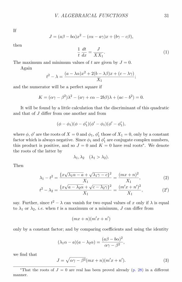
If
J = (aβ − bα)x2 − (cα− aγ)x+ (bγ − cβ),
then1
t
dt
dx=
J
XX1. (1)
The maximum and minimum values of t are given by J = 0.
Again
t2 − λ =(a− λα)x2 + 2(b− λβ)x+ (c− λγ)
X1;
and the numerator will be a perfect square if
K = (αγ − β2)λ2 − (aγ + cα− 2bβ)λ+ (ac− b2) = 0.
It will be found by a little calculation that the discriminant of this quadraticand that of J differ from one another and from
(φ− φ1)(φ− φ′1)(φ′ − φ1)(φ′ − φ′1),
where φ, φ′ are the roots of X = 0 and φ1, φ′1 those of X1 = 0, only by a constant
factor which is always negative. Since φ1 and φ′1 are conjugate complex numbers,this product is positive, and so J = 0 and K = 0 have real roots∗. We denotethe roots of the latter by
λ1, λ2 (λ1 > λ2).
Then
λ1 − t2 =x√λ1α− a+
√λ1γ − c2
X1=
(mx+ n)2
X1, (2)
t2 − λ2 =x√a− λ2α+
√c− λ2γ2
X1=
(m′x+ n′)2
X1, (2′)
say. Further, since t2 − λ can vanish for two equal values of x only if λ is equalto λ1 or λ2, i.e. when t is a maximum or a minimum, J can differ from
(mx+ n)(m′x+ n′)
only by a constant factor; and by comparing coefficients and using the identity
(λ1α− a)(a− λ2α) =(aβ − bα)2
αγ − β2,
we find that
J =√αγ − β2(mx+ n)(m′x+ n′). (3)
∗That the roots of J = 0 are real has been proved already (p. 28) in a differentmanner.
V. ALGEBRAICAL FUNCTIONS 32
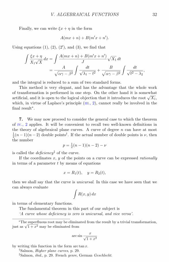
Finally, we can write ξx+ η in the form
A(mx+ n) +B(m′x+ n′).
Using equations (1), (2), (2′), and (3), we find that∫ξx+ η
X1
√Xdx =
∫A(mx+ n) +B(m′x+ n′)
J
√X1 dt
=A√
αγ − β2
∫dt√
λ1 − t2+
B√αγ − β2
∫dt√
t2 − λ2,
and the integral is reduced to a sum of two standard forms.This method is very elegant, and has the advantage that the whole work
of transformation is performed in one step. On the other hand it is somewhatartificial, and it is open to the logical objection that it introduces the root
√X1,
which, in virtue of Laplace’s principle (iii., 2), cannot really be involved in thefinal result∗.
7. We may now proceed to consider the general case to which the theoremof iv., 2 applies. It will be convenient to recall two well-known definitions inthe theory of algebraical plane curves. A curve of degree n can have at most12(n− 1)(n− 2) double points†. If the actual number of double points is ν, thenthe number
p = 12(n− 1)(n− 2)− ν
is called the deficiency‡ of the curve.If the coordinates x, y of the points on a curve can be expressed rationally
in terms of a parameter t by means of equations
x = R1(t), y = R2(t),
then we shall say that the curve is unicursal. In this case we have seen that wecan always evaluate ∫
R(x, y) dx
in terms of elementary functions.The fundamental theorem in this part of our subject is‘A curve whose deficiency is zero is unicursal, and vice versa’.
∗The superfluous root may be eliminated from the result by a trivial transformation,just as
√1 + x2 may be eliminated from
arc sinx√
1 + x2
by writing this function in the form arc tanx.†Salmon, Higher plane curves, p. 29.‡Salmon, ibid., p. 29. French genre, German Geschlecht.

V. ALGEBRAICAL FUNCTIONS 33
Suppose first that the curve possesses the maximum number of doublepoints∗. Since
12(n− 1)(n− 2) + n− 3 = 1
2(n− 2)(n+ 1)− 1,
and 12(n − 2)(n + 1) points are just sufficient to determine a curve of degree
n− 2†, we can draw, through the 12(n− 1)(n− 2) double points and n− 3 other
points chosen arbitrarily on the curve, a simply infinite set of curves ofdegree n− 2, which we may suppose to have the equation
g(x, y) + t h(x, y) = 0,
where t is a variable parameter and g = 0, h = 0 are the equations of twoparticular members of the set. Any one of these curves meets the given curve inn(n− 2) points, of which (n− 1)(n− 2) are accounted for by the 1
2(n− 1)(n− 2)double points, and n− 3 by the other n− 3 arbitrarily chosen points. These
(n− 1)(n− 2) + n− 3 = n(n− 2)− 1
points are independent of t; and so there is but one point of intersection whichdepends on t. The coordinates of this point are given by
g(x, y) + t h(x, y) = 0, f(x, y) = 0.
The elimination of y gives an equation of degree n(n−2) in x, whose coefficientsare polynomials in t; and but one root of this equation varies with t. Theeliminant is therefore divisible by a factor of degree n(n− 2)− 1 which doesnot contain t. There remains a simple equation in x whose coefficients arepolynomials in t. Thus the x-coordinate of the variable point is determined asa rational function of t, and the y-coordinate may be similarly determined.
We may therefore write
x = R1(t), y = R2(t).
If we reduce these fractions to the same denominator, we express the coordinatesin the form
x =φ1(t)
φ3(t), y =
φ2(t)
φ3(t), (1)
∗We suppose in what follows that the singularities of the curve are all ordinarynodes. The necessary modifications when this is not the case are not difficult to make.An ordinary multiple point of order k may be regarded as equivalent to 1
2k(k − 1)ordinary double points. A curve of degree n which has an ordinary multiple point oforder n−1, equivalent to 1
2 (n−1)(n−2) ordinary double points, is therefore unicursal.The theory of higher plane curves abounds in puzzling particular cases which have tobe fitted into the general theory by more or less obvious conventions, and to give asatisfactory account of a complicated compound singularity is sometimes by no meanseasy. In the investigation which follows we confine ourselves to the simplest case.
†Salmon, l.c., p. 16.

V. ALGEBRAICAL FUNCTIONS 34
where φ1, φ2, φ3 are polynomials which have no common factor. Thepolynomials will in general be of degree n; none of them can be of higherdegree, and one at least must be actually of that degree, since an arbitrarystraight line
λx+ µy + ν = 0
must cut the curve in exactly n points∗.
We can now prove the second part of the theorem. If
x : y : 1 :: φ1(t) : φ2(t) : φ3(t),
where φ1, φ2, φ3 are polynomials of degree n, then the line
ux+ vy + w = 0
will meet the curve in n points whose parameters are given by
uφ1(t) + vφ2(t) + wφ3(t) = 0.
This equation will have a double root t0 if
uφ1(t0) + vφ2(t0) + wφ3(t0) = 0,
uφ′1(t0) + vφ′2(t0) + wφ′3(t0) = 0.
Hence the equation of the tangent at the point t0 is∣∣∣∣∣∣x y 1
φ1(t0) φ2(t0) φ3(t0)φ′1(t0) φ′2(t0) φ′3(t0)
∣∣∣∣∣∣ = 0. (2)
If (x, y) is a fixed point, then the equation (2) may be regarded as anequation to determine the parameters of the points of contact of the tangentsfrom (x, y). Now
φ2(t0)φ′3(t0)− φ′2(t0)φ3(t0)
is of degree 2n− 2 in t0, the coefficient of t2n−10 obviously vanishing. Hence ingeneral the number of tangents which can be drawn to a unicursal curve froma fixed point (the class of the curve) is 2n− 2. But the class of a curve whose
∗See Niewenglowski’s Cours de geometrie analytique, vol. 2, p. 103. By way ofillustration of the remark concerning particular cases in the footnote (§) to page 30,the reader may consider the example given by Niewenglowski in which
x =t2
t2 − 1, y =
t2 + 1
t2 − 1;
equations which appear to represent the straight line 2x = y + 1 (part of the lineonly, if we consider only real values of t).

V. ALGEBRAICAL FUNCTIONS 35
only singular points are δ nodes is known∗ to be n(n − 1) − 2δ. Hence thenumber of nodes is
12n(n− 1)− (2n− 2) = 1
2(n− 1)(n− 2).
It is perhaps worth pointing out how the proof which precedes requiresmodification if some only of the singular points are nodes and the rest ordinarycusps. The first part of the proof remains unaltered. The equation (2) mustnow be regarded as giving the values of t which correspond to (a) points atwhich the tangent passes through (x, y) and (b) cusps, since any line througha cusp ‘cuts the curve in two coincident points’†. We have therefore
2n− 2 = m+ κ,
where m is the class of the curve. But
m = n(n− 1)− 2δ − 3κ, ‡
and so
δ + κ = 12(n− 1)(n− 2).§
8. (i) The preceding argument fails if n < 3, but we have already seenthat all conics are unicursal. The case next in importance is that of a cubicwith a double point. If the double point is not at infinity we can, by a changeof origin, reduce the equation of the curve to the form
(ax+ by)(cx+ dy) = px3 + 3qx2y + 3rxy2 + sy3;
and, by considering the intersections of the curve with the line y = tx, we find
x =(a+ bt)(c+ dt)
p+ 3qt+ 3rt2 + st3, y =
t(a+ bt)(c+ dt)
p+ 3qt+ 3rt2 + st3.
If the double point is at infinity, the equation of the curve is of the form
(αx+ βy)2(γx+ δy) + εx+ ζy + θ = 0,
∗Salmon, l.c., p. 54.†This means of course that the equation obtained by substituting for x and y, in
the equation of the line, their parametric expressions in terms of t, has a repeatedroot. This property is possessed by the tangent at an ordinary point and by any linethrough a cusp, but not by any line through a node except the two tangents.
‡Salmon, l.c., p. 65.§I owe this remark to Mr A. B. Mayne. Dr Bromwich has however pointed out to
me that substantially the same argument is given by Mr W. A. Houston, ‘Note onunicursal plane curves’, Messenger of mathematics, vol. 28, 1899, pp. 187–189.

V. ALGEBRAICAL FUNCTIONS 36
the curve having a pair of parallel asymptotes; and, by considering theintersection of the curve with the line αx+ βy = t, we find
x = − δt3 + ζt+ βθ
(βγ − αδ)t2 + εβ − αζ, y =
γt3 + εt+ αθ
(βγ − αδ)t2 + εβ − αζ.
(ii) The case next in complexity is that of a quartic with three doublepoints.
(a) The lemniscate
(x2 + y2)2 = a2(x2 − y2)
has three double points, the origin and the circular points at infinity. The circle
x2 + y2 = t(x− y)
passes through these points and one other fixed point at the origin, as ittouches the curve there. Solving, we find
x =a2t(t2 + a2)
t4 + a4, y =
a2t(t2 − a2)t4 + a4
.
(b) The curve2ay3 − 3a2y2 = x4 − 2a2x2
has the double points (0, 0), (a, a), (−a, a). Using the auxiliary conic
x2 − ay = tx(y − a),
we findx =
a
t3(2− 3t2), y =
a
2t4(2− 3t2)(2− t2).
(iii) (a) The curveyn = xn + axn−1
has a multiple point of order n− 1 at the origin, and is therefore unicursal. Inthis case it is sufficient to consider the intersection of the curve with the liney = tx. This may be harmonised with the general theory by regarding the curve
yn−3(y − tx) = 0,
as passing through each of the 12(n− 1)(n− 2) double points collected at the
origin and through n− 3 other fixed points collected at the point
x = −a, y = 0.
The curves
yn = xn + axn−1, (1)
yn = 1 + az, (2)

V. ALGEBRAICAL FUNCTIONS 37
are projectively equivalent, as appears on rendering their equations homogeneousby the introduction of variables z in (1) and x in (2). We conclude that (2) isunicursal, having the maximum number of double points at infinity. In fact wemay put
y = t, az = tn − 1.
The integral ∫Rz, n
√1 + az dz
is accordingly an elementary function.(b) The curve
ym = A(x− a)µ(x− b)ν
is unicursal if and only if either (i) µ = 0 or (ii) ν = 0 or (iii) µ+ ν = m. Hencethe integral ∫
Rx, (x− a)µ/m(x− b)ν/n dx
is an elementary function, for all forms of R, in these three cases only; ofcourse it is integrable for special forms of R in other cases∗.
9. There is a similar theory connected with unicursal curves in space ofany number of dimensions. Consider for example the integral∫
Rx,√ax+ b,
√cx+ d dx.
A linear substitution y = lx+m reduces this integral to the form∫R1y,
√y + 2,
√y − 2 dy;
and this integral can be rationalised by putting
y = t2 +1
t2,√y + 2 = t+
1
t,√y − 2 = t− 1
t.
The curve whose Cartesian coordinates ξ, η, ζ are given by
ξ : η : ζ : 1 :: t4 + 1 : t(t2 + 1) : t(t2 − 1) : t2,
is a unicursal twisted quartic, the intersection of the parabolic cylinders
ξ = η2 − 2, ξ = ζ2 + 2.
It is easy to deduce that the integral∫R
x,
√ax+ b
mx+ n,
√cx+ d
mx+ n
dx
is always an elementary function.
∗See Ptaszycki, ‘Extrait d’une lettre adressee a M. Hermite’, Bulletin des sciencesmathematiques, ser. 2, vol. 12, 1888, pp. 262–270: Appell and Goursat, Theorie desfonctions algebriques, p. 245.

V. ALGEBRAICAL FUNCTIONS 38
10. When the deficiency of the curve f(x, y) = 0 is not zero, the integral∫R(x, y) dx
is in general not an elementary function; and the consideration of such integralshas consequently introduced a whole series of classes of new transcendents intoanalysis. The simplest case is that in which the deficiency is unity: in this case,as we shall see later on, the integrals are expressible in terms of elementaryfunctions and certain new transcendents known as elliptic integrals. When thedeficiency rises above unity the integration necessitates the introduction of newtranscendents of growing complexity.
But there are infinitely many particular cases in which integrals, associatedwith curves whose deficiency is unity or greater than unity, can be expressed interms of elementary functions, or are even algebraical themselves. For instancethe deficiency of
y2 = 1 + x3
is unity. But ∫x+ 1
x− 2
dx√1 + x3
= 3 log(1 + x)2 − 3
√1 + x3
(1 + x)2 + 3√
1 + x3,∫
2− x3
1 + x3dx√
1 + x3=
2x√1 + x3
.
And, before we say anything concerning the new transcendents to whichintegrals of this class in general give rise, we shall consider what has beendone in the way of formulating rules to enable us to identify such cases and toassign the form of the integral when it is an elementary function. It will be aswell to say at once that this problem has not been solved completely.
11. The first general theorem of this character deals with the case inwhich the integral is algebraical, and asserts that if
u =
∫y dx
is an algebraical function of x, then it is a rational function of x and y.
Our proof will be based on the following lemmas.(1) If f(x, y) and g(x, y) are polynomials, and there is no factor common
to all the coefficients of the various powers of y in g(x, y); and
f(x, y) = g(x, y)h(x),
where h(x) is a rational function of x; then h(x) is a polynomial.
Let h = P/Q, where P and Q are polynomials without a common factor.Then
fQ = gP.

V. ALGEBRAICAL FUNCTIONS 39
If x− a is a factor of Q, then
g(a, y) = 0
for all values of y; and so all the coefficients of powers of y in g(x, y) aredivisible by x− a, which is contrary to our hypotheses. Hence Q is a constantand h a polynomial.
(2) Suppose that f(x, y) is an irreducible polynomial, and that y1, y2, . . . ,yn are the roots of
f(x, y) = 0
in a certain domain D. Suppose further that φ(x, y) is another polynomial, andthat
φ(x, y1) = 0.
Then
φ(x, ys) = 0,
where ys is any one of the roots of (1); and
φ(x, y) = f(x, y)ψ(x, y),
where ψ(x, y) also is a polynomial in x and y.
Let us determine the highest common factor $ of f and φ, considered aspolynomials in y, by the ordinary process for the determination of the highestcommon factor of two polynomials. This process depends only on a series ofalgebraical divisions, and so $ is a polynomial in y with coefficients rationalin x. We have therefore
$(x, y) = ω(x, y)λ(x), (1)
f(x, y) = ω(x, y)p(x, y)µ(x) = g(x, y)µ(x), (2)
φ(x, y) = ω(x, y)q(x, y)ν(x) = h(x, y)ν(x), (3)
where ω, p, q, g, and h are polynomials and λ, µ, and ν rational functions; andevidently we may suppose that neither in g nor in h have the coefficients of allpowers of y a common factor. Hence, by Lemma (1), µ and ν are polynomials.But f is irreducible, and therefore µ and either ω or p must be constants. Ifω were a constant, $ would be a function of x only. But this is impossible.For we can determine polynomials L, M in y, with coefficients rational in x,such that
Lf +Mφ = $, (4)
and the left-hand side of (4) vanishes when we write y1 for y. Hence p is aconstant, and so ω is a constant multiple of f . The truth of the lemma nowfollows from (3).
It follows from Lemma (2) that y cannot satisfy any equation of degree lessthan n whose coefficients are polynomials in x.

V. ALGEBRAICAL FUNCTIONS 40
(3) If y is an algebraical function of x, defined by an equation
f(x, y) = 0 (1)
of degree n, then any rational function R(x, y) of x and y can be expressed inthe form
R(x, y) = R0 +R1y + · · ·+Rn−1yn−1, (2)
where R0, R1, . . . , Rn−1 are rational functions of x.
The function y is one of the n roots of (1). Let y, y′, y′′, . . . be thecomplete system of roots. Then
R(x, y) =P (x, y)
Q(x, y)
=P (x, y)Q(x, y′)Q(x, y′′) . . .
Q(x, y)Q(x, y′)Q(x, y′′) . . ., (3)
where P and Q are polynomials. The denominator is a polynomial in x whosecoefficients are symmetric polynomials in y, y′, y′′, . . . , and is therefore, byii., §3, (i), a rational function of x. On the other hand
Q(x, y′)Q(x, y′′) . . .
is a polynomial in x whose coefficients are symmetric polynomials in y′, y′′, . . . ,and therefore, by ii., §3, (ii), polynomials in y with coefficients rational in x.Thus the numerator of (3) is a polynomial in y with coefficients rational in x.
It follows that R(x, y) is a polynomial in y with coefficients rational in x.From this polynomial we can eliminate, by means of (1), all powers of y ashigh as or higher than the nth. Hence R(x, y) is of the form prescribed by thelemma.
12. We proceed now to the proof of our main theorem. We have∫y dx = u
where u is algebraical. Let
f(x, y) = 0, ψ(x, u) = 0 (1)
be the irreducible equations satisfied by y and u, and let us suppose that theyare of degrees n and m respectively. The first stage in the proof consists inshowing that
m = n.
It will be convenient now to write y1, u1 for y, u, and to denote by
y1, y2, . . . , yn, u1, u2, . . . , um,

V. ALGEBRAICAL FUNCTIONS 41
the complete systems of roots of the equations (1).We have
ψ(x, u1) = 0,
and so
χ1 =∂ψ
∂x+∂ψ
∂u1
du1dx
=∂ψ
∂x+ y1
∂ψ
∂u1= 0.
Now let
Ω(x, u1) =n∏r=1
(∂ψ
∂x+ yr
∂ψ
∂u1
).
Then Ω is a polynomial in u1, with coefficients symmetric in y1, y2, . . . , ynand therefore rational in x.
The equations ψ = 0 and Ω = 0 have a root u1 in common, and the firstequation is irreducible. It follows, by Lemma (2) of §11, that
Ω(x, us) = 0
for s = 1, 2, . . . , m.∗ And from this it follows that, when s is given, we have
∂ψ
∂x+ yr
∂ψ
∂us(2)
for some value of the suffix r.But we have also
∂ψ
∂x+∂ψ
∂us
dusdx
= 0; (3)
and from (2) and (3) it follows† that
dusdx
= yr, (4)
i.e. that every u is the integral of some y.In the same way we can show that every y is the derivative of some u. Let
ω(x, y1) =
m∏s=1
(∂ψ
∂x+ y1
∂ψ
∂us
).
∗If p(x) is the least common multiple of the denominators of the coefficients ofpowers of u in Ω, then
Ω(x, u)p(x) = χ(x, u),
where χ is a polynomial. Applying Lemma (2), we see that χ(x, us) = 0, and so
Ω(x, us) = 0.
†It is impossible that ψ and∂ψ
∂ushould both vanish for u = us, since ψ is
irreducible.

V. ALGEBRAICAL FUNCTIONS 42
Then ω is a polynomial in y1, with coefficients symmetric in u1, u2, . . . , umand therefore rational in x. The equations f = 0 and ω = 0 have a root y1 incommon, and so
ω(x, yr) = 0
for r = 1, 2, . . . , n. From this we deduce that, when r is given, (2) must betrue for some value of s, and so that the same is true of (4).
Now it is impossible that, in (4), two different values of s should correspondto the same value of r. For this would involve
us − ut = c
where s 6= t and c is a constant. Hence we should have
ψ(x, us) = 0, ψ(x, us − c) = 0.
Subtracting these equations, we should obtain an equation of degree m − 1in us, with coefficients which are polynomials in x; and this is impossible. Inthe same way we can prove that two different values of r cannot correspond tothe same value of s.
The equation (4) therefore establishes a one-one correspondence betweenthe values of r and s. It follows that
m = n.
It is moreover evident that, by arranging the suffixes properly, we can make
durdx
= yr (5)
for r = 1, 2, . . . , n.
13. We have
yr =durdx
= −∂ψ∂x
/∂ψ
∂ur= R(x, ur),
where R is a rational function which may, in virtue of Lemma (3) of § 11, beexpressed as a polynomial of degree n− 1 in ur, with coefficients rational in x.
The product ∏s 6=r
(z − ys)
is a polynomial of degree n − 1 in z, with coefficients which are symmetricpolynomials in y1, y2, . . . , yr−1, yr+1, . . . , yn and therefore, by ii., §3, (ii),polynomials in yr with coefficients rational in x. Replacing yr by its expressionas a polynomial in ur obtained above, and eliminating unr and all higher powersof ur, we obtain an equation
∏s 6=r
(z − ys) =n−1∑j=0
n−1∑k=0
Sj,k(x)zjukr ,

V. ALGEBRAICAL FUNCTIONS 43
where the S’s are rational functions of x which are, from the method of theirformation, independent of the particular value of r selected. We may thereforewrite ∏
s 6=r(z − ys) = P (x, z, ur),
where P is a polynomial in z and ur with coefficients rational in x. It isevident that
P (x, ys, ur) = 0
for every value of s other than r. In particular
P (x, y1, ur) = 0 (r = 2, 3, . . . , n).
It follows that the n− 1 roots of the equation in u
P (x, y1, u) = 0
are u2, u3, . . . , un. We have therefore
P (x, y1, u) = T0(x, y1)
n∏2
(u− ur)
= T0(x, y1)un−1 − un−2(u2 + u3 + · · ·+ un) + . . .
= T0(x, y1)
[un−1 + un−2
u1 +
B1(x)
B0(x)
+ . . .
],
where T0(x, y1) is the coefficient of un−1 in P , and B0(x) and B1(x) are thecoefficients of un and un−1 in ψ. Equating the coefficients of un−2 on the twosides of this equation, we obtain
u1 +B1(x)
B0(x)=T1(x, y1)
T0(x, y1),
where T1(x, y1) is the coefficient of un−2 in P . Thus the theorem is proved.
14. We can now apply Lemma (3) of §11; and we arrive at the finalconclusion that if ∫
y dx
is algebraical then it can be expressed in the form
R0 +R1y + · · ·+Rn−1yn−1,
where R0, R1, . . . are rational functions of x.
The most important case is that in which
y = n√R(x),

V. ALGEBRAICAL FUNCTIONS 44
where R(x) is rational. In this case
yn = R(x), (1)
dy
dx=R′(x)
nyn−1. (2)
But
y = R′0 +R′1y + · · ·+R′n−1yn−1
+ R1 + 2R2y + · · ·+ (n− 1)Rn−1yn−2 dy
dx. (3)
Eliminatingdy
dxbetween these equations, we obtain an equation
$(x, y) = 0, (4)
where $(x, y) is a polynomial. It follows from Lemma (2) of §11 that thisequation must be satisfied by all the roots of (1). Thus (4) is still true if wereplace y by any other root y′ of (1); and as (2) is still true when we effect thissubstitution, it follows that (3) is also still true. Integrating, we see that theequation ∫
y dx = R0 +R1y + · · ·+Rn−1yn−1
is true when y is replaced by y′. We may therefore replace y by ωy, ω beingany primitive nth root of unity. Making this substitution, and multiplyingby ωn−1, we obtain∫
y dx = ωn−1R0 +R1y + ωR2y + · · ·+ ωn−2Rn−1yn−1;
and on adding the n equations of this type we obtain∫y dx = R1y.
Thus in this case the functions R0, R2, . . . , Rn−1 all disappear.
It has been shown by Liouville∗ that the preceding results enable us toobtain in all cases, by a finite number of elementary algebraical operations, asolution of the problem ‘to determine whether
∫y dx is algebraical, and to find
the integral when it is algebraical ’.
∗‘Premier memoire sur la determination des integrales dont la valeur estalgebrique’, Journal de l’Ecole Polytechnique, vol. 14, cahier 22, 1833, pp. 124–148;‘Second memoire. . . ’, ibid., pp. 149–193.

V. ALGEBRAICAL FUNCTIONS 45
15. It would take too long to attempt to trace in detail the steps of thegeneral argument. We shall confine ourselves to a solution of a particularproblem which will give a sufficient illustration of the general nature of thearguments which must be employed.
We shall determine under what circumstances the integral∫dx
(x− p)√ax2 + 2bx+ c
is algebraical. This question might of course be answered by actually evaluatingthe integral in the general case and finding when the integral function reducesto an algebraical function. We are now, however, in a position to answer itwithout any such integration.
We shall suppose first that ax2 + 2bx+ c is not a perfect square. In this case
y =1√X,
whereX = (x− p)2(ax2 + 2bx+ c),
and if∫y dx is algebraical it must be of the form
R(x)√X.
Hence
y =d
dx
(R√X
),
or2X = 2XR′ −RX ′.
We can now show that R is a polynomial in x. For if R = U/V , where Uand V are polynomials, then V , if not a mere constant, must contain a factor
(x− α)µ (µ > 0),
and we can put
R =U
W (x− α)µ,
where U and W do not contain the factor x− α. Substituting this expressionfor R, and reducing, we obtain
2µUWX
x− α= 2U ′WX − 2UW ′X − UWX ′ − 2W 2X(x− α)µ.
Hence X must be divisible by x− α. Suppose then that
X = (x− α)kY,

V. ALGEBRAICAL FUNCTIONS 46
where Y is prime to x − α. Substituting in the equation last obtained wededuce
(2µ+ k)UWY
x− α= 2U ′WY − 2UW ′Y − UWY ′ − 2W 2Y (x− α)µ,
which is obviously impossible, since neither U , W , nor Y is divisible by x− α.Thus V must be a constant. Hence∫
dx
(x− p)√ax2 + 2bx+ c
=U(x)
(x− p)√ax2 + 2bx+ c
,
where U(x) is a polynomial.Differentiating and clearing of radicals we obtain
(x− p)(U ′ − 1)− U(ax2 + 2bx+ c) = U(x− p)(ax+ b).
Suppose that the first term in U is Axm. Equating the coefficients of xm+2, wefind at once that m = 2. We may therefore take
U = Ax2 + 2Bx+ C,
so that
(x− p)(2Ax+ 2B − 1)−Ax2 − 2Bx− C(ax2 + 2bx+ c)
= (x− p)(ax+ b)(Ax2 + 2Bx+ C). (1)
From (1) it follows that
(x− p)(ax+ b)(Ax2 + 2Bx+ C)
is divisible by ax2 + 2bx+ c. But ax+ b is not a factor of ax2 + 2bx+ c, as thelatter is not a perfect square. Hence either (i) ax2 + 2bx+ c and Ax2 + 2Bx+Cdiffer only by a constant factor or (ii) the two quadratics have one and onlyone factor in common, and x− p is also a factor of ax2 + 2bx+ c. In the lattercase we may write
ax2 + 2bx+ c = a(x− p)(x− q), Ax2 + 2Bx+ C = A(x− q)(x− r),
where p 6= q, p 6= r. It then follows from (1) that
a(x− p)(2Ax+ 2B − 1)− aA(x− q)(x− r) = A(ax+ b)(x− r).
Hence 2Ax+ 2B − 1 is divisible by x− r. Dividing by aA(x− r) we obtain
2(x− p)− (x− q) = x+b
a= x− 1
2(p+ q),
and so p = q, which is untrue.

V. ALGEBRAICAL FUNCTIONS 47
Hence case (ii) is impossible, and so ax2 + 2bx + c and Ax2 + 2Bx + Cdiffer only by a constant factor. It then follows from (1) that x− p is a factorof ax2 + 2bx+ c; and the result becomes∫
dx
(x− p)√ax2 + 2bx+ c
= K
√ax2 + 2bx+ c
x− p,
where K is a constant. It is easily verified that this equation is actually truewhen ap2 + 2bp+ c = 0, and that
K =1√
b2 − ac.
The formula is equivalent to∫dx
(x− p)√
(x− p)(x− q)=
2
q − p
√x− qx− p
.
There remains for consideration the case in which ax2 + 2bx+ c is a perfectsquare, say a(x− q)2. Then ∫
dx
(x− p)(x− q)must be rational, and so p = q.
As a further example, the reader may verify that if
y3 − 3y + 2x = 0
then ∫y dx =
3
8(2xy − y2).∗
16. The theorem of §11 enables us to complete the proof of the twofundamental theorems stated without proof in ii., §5, viz.
(a) ex is not an algebraical function of x,(b) log x is not an algebraical function of x.We shall prove (b) as a special case of a more general theorem, viz. ‘no
sum of the formA log(x− α) +B log(x− β) + . . . ,
in which the coefficients A, B, . . . are not all zero, can be an algebraicalfunction of x’. To prove this we have only to observe that the sum in questionis the integral of a rational function of x. If then it is algebraical it must,by the theorem of §11, be rational, and this we have already seen to beimpossible (iv., 2).
That ex is not algebraical now follows at once from the fact that it is theinverse function of log x.
∗Raffy, ‘Sur les quadratures algebriques et logarithmiques’, Annales de l’EcoleNormale, ser. 3, vol. 2, 1885, pp. 185–206.

V. ALGEBRAICAL FUNCTIONS 48
17. The general theorem of §11 gives the first step in the rigid proof of‘Laplace’s principle’ stated in iii., §2. On account of the immense importance ofthis principle we repeat Laplace’s words: ‘l’integrale d’une fonction differentiellene peut contenir d’autres quantites radicales que celles qui entrent dans cettefonction’. This general principle, combined with arguments similar to thoseused above (§15) in a particular case, enables us to prove without difficultythat a great many integrals cannot be algebraical, notably the standard ellipticintegrals∫
dx√(1− x2)(1− k2x2)
,
∫ √1− x2
1− k2x2dx,
∫dx√
4x3 − g2x− g3which give rise by inversion to the elliptic functions.
18. We must now consider in a very summary manner the more difficultquestion of the nature of those integrals of algebraical functions which areexpressible in finite terms by means of the elementary transcendental functions.In the first place no integral of any algebraical function can contain anyexponential. Of this theorem it is, as we remarked before, easy to becomeconvinced by a little reflection, as doubtless did Laplace, who certainlypossessed no rigorous proof. The reader will find little difficulty in comingto the conclusion that exponentials cannot be eliminated from an elementaryfunction by differentiation. But we would strongly recommend him to studythe exceedingly beautiful and ingenious proof of this proposition given byLiouville∗. We have unfortunately no space to insert it here.
It is instructive to consider particular cases of this theorem. Suppose forexample that
∫y dx, where y is algebraical, were a polynomial in x and ex, say∑∑
am,nxmenx. (1)
When this expression is differentiated, ex must disappear from it: otherwisewe should have an algebraical relation between x and ex. Expressing theconditions that the coefficient of every power of ex in the differential coefficientof (1) vanishes identically, we find that the same must be true of (1), so thatafter all the integral does not really contain ex. Liouville’s proof is in reality adevelopment of this idea.
The integral of an algebraical function, if expressible in terms of elementaryfunctions, can therefore only contain algebraical or logarithmic functions.The next step is to show that the logarithms must be simple logarithms ofalgebraical functions and can only enter linearly, so that the general integralmust be of the type ∫
y dx = u+A log v +B logw + . . . ,
∗‘Memoire sur les transcendantes elliptiques considerees comme fonctions de leuramplitude’, Journal de l’Ecole Polytechnique, vol. 14, cahier 23, 1834, pp. 37–83. Theproof may also be found in Bertrand’s Calcul integral, p. 99.

V. ALGEBRAICAL FUNCTIONS 49
where A, B, . . . are constants and u, v, w, . . . algebraical functions. Only whenthe logarithms occur in this simple form will differentiation eliminate them.
Lastly it can be shown by arguments similar to those of §§11–14 that u, v,w, . . . are rational functions of x and y. Thus
∫y dx, if an elementary function,
is the sum of a rational function of x and y and of certain constant multiples oflogarithms of such functions. We can suppose that no two of A, B, . . . arecommensurable, or indeed, more generally, that no linear relation
Aα+Bβ + · · · = 0,
with rational coefficients, holds between them. For if such a relation held thenwe could eliminate A from the integral, writing it in the form∫
y dx = u+B log(wv−β/α) + . . . .
It is instructive to verify the truth of this theorem in the special case inwhich the curve f(x, y) = 0 is unicursal. In this case x and y are rationalfunctions R(t), S(t) of a parameter t, and the integral, being the integral of arational function of t, is of the form
u+A log v +B logw + . . . ,
where u, v, w, . . . are rational functions of t. But t may be expressed, bymeans of elementary algebraical operations, as a rational function of x and y.Thus u, v, w, . . . are rational functions of x and y.
The case of greatest interest is that in which y is a rational function ofx and
√X, where X is a polynomial. As we have already seen, y can in this
case be expressed in the form
P +Q√X,
where P and Q are rational functions of x. We shall suppress the rational partand suppose that y = Q/
√X. In this case the general theorem gives∫
Q√Xdx = S +
T√X
+A log(α+ β√X) +B log(γ + δ
√X) + . . . ,
where S, T , α, β, γ, δ, . . . are rational. If we differentiate this equation weobtain an algebraical identity in which we can change the sign of
√X. Thus
we may change the sign of√X in the integral equation. If we do this and
subtract, and write 2A, . . . for A, . . . , we obtain∫Q√Xdx =
T√X
+A logα+ β
√X
α− β√X
+B logγ + δ
√X
γ − δ√X
+ . . . ,
which is the standard form for such an integral. It is evident that we maysuppose α, β, γ, . . . to be polynomials.

V. ALGEBRAICAL FUNCTIONS 50
19. (i) By means of this theorem it is possible to prove that a numberof important integrals, and notably the integrals∫
dx√(1− x2)(1− k2x2)
,
∫ √1− x2
1− k2x2dx,
∫dx√
4x3 − g2x− g3,
are not expressible in terms of elementary functions, and so represent genuinelynew transcendents. The formal proof of this was worked out by Liouville∗;
it rests merely on a consideration of the possible forms of the differentialcoefficients of expressions of the form
T√X
+A logα+ β
√X
α− β√X
+ . . . ,
and the arguments used are purely algebraical and of no great theoreticaldifficulty. The proof is however too detailed to be inserted here. It is notdifficult to find shorter proofs, but these are of a less elementary character,being based on ideas drawn from the theory of functions†.
The general questions of this nature which arise in connection with integralsof the form ∫
Q√Xdx,
or, more generally, ∫Qm√Xdx,
are of extreme interest and difficulty. The case which has received mostattention is that in which m = 2 and X is of the third or fourth degree,in which case the integral is said to be elliptic. An integral of this kind iscalled pseudo-elliptic if it is expressible in terms of algebraical and logarithmicfunctions. Two examples were given above (§ 10). General methods havebeen given for the construction of such integrals, and it has been shown thatcertain interesting forms are pseudo-elliptic. In Goursat’s Cours d’analyse‡,for instance, it is shown that if f(x) is a rational function such that
f(x) + f
(1
k2x
)= 0,
then ∫f(x) dx√
x(1− x)(1− k2x)
∗See Liouville’s memoir quoted on p. 45 (pp. 45 et seq.).†The proof given by Laurent (Traite d’analyse, vol. 4, pp. 153 et seq.) appears at
first sight to combine the advantages of both methods of proof, but unfortunatelywill not bear a closer examination.
‡Second edition, vol. 1, pp. 267–269.
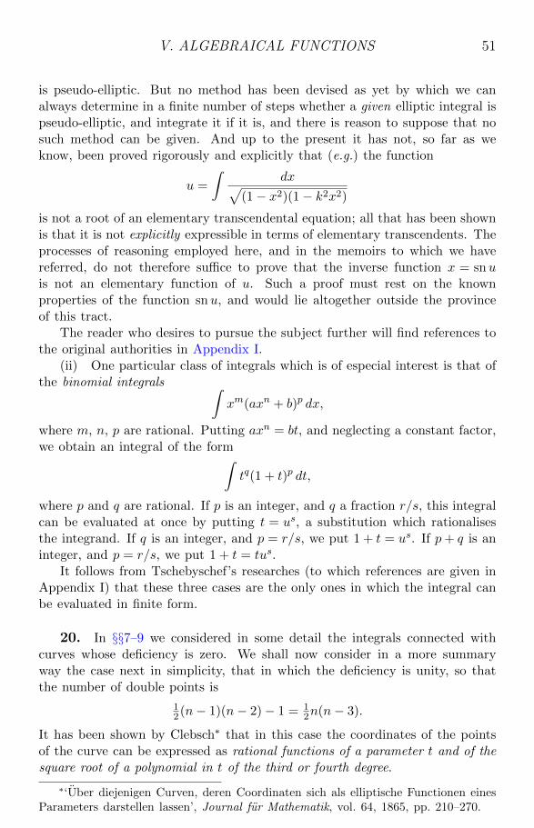
V. ALGEBRAICAL FUNCTIONS 51
is pseudo-elliptic. But no method has been devised as yet by which we canalways determine in a finite number of steps whether a given elliptic integral ispseudo-elliptic, and integrate it if it is, and there is reason to suppose that nosuch method can be given. And up to the present it has not, so far as weknow, been proved rigorously and explicitly that (e.g.) the function
u =
∫dx√
(1− x2)(1− k2x2)is not a root of an elementary transcendental equation; all that has been shownis that it is not explicitly expressible in terms of elementary transcendents. Theprocesses of reasoning employed here, and in the memoirs to which we havereferred, do not therefore suffice to prove that the inverse function x = snuis not an elementary function of u. Such a proof must rest on the knownproperties of the function snu, and would lie altogether outside the provinceof this tract.
The reader who desires to pursue the subject further will find references tothe original authorities in Appendix I.
(ii) One particular class of integrals which is of especial interest is that ofthe binomial integrals ∫
xm(axn + b)p dx,
where m, n, p are rational. Putting axn = bt, and neglecting a constant factor,we obtain an integral of the form∫
tq(1 + t)p dt,
where p and q are rational. If p is an integer, and q a fraction r/s, this integralcan be evaluated at once by putting t = us, a substitution which rationalisesthe integrand. If q is an integer, and p = r/s, we put 1 + t = us. If p+ q is aninteger, and p = r/s, we put 1 + t = tus.
It follows from Tschebyschef’s researches (to which references are given inAppendix I) that these three cases are the only ones in which the integral canbe evaluated in finite form.
20. In §§7–9 we considered in some detail the integrals connected withcurves whose deficiency is zero. We shall now consider in a more summaryway the case next in simplicity, that in which the deficiency is unity, so thatthe number of double points is
12(n− 1)(n− 2)− 1 = 1
2n(n− 3).
It has been shown by Clebsch∗ that in this case the coordinates of the pointsof the curve can be expressed as rational functions of a parameter t and of thesquare root of a polynomial in t of the third or fourth degree.
∗‘Uber diejenigen Curven, deren Coordinaten sich als elliptische Functionen einesParameters darstellen lassen’, Journal fur Mathematik, vol. 64, 1865, pp. 210–270.

V. ALGEBRAICAL FUNCTIONS 52
The fact is that the curves
y2 = a+ bx+ cx2 + dx3,
y2 = a+ bx+ cx2 + dx3 + ex4,
are the simplest curves of deficiency 1. The first is the typical cubic withouta double point. The second is a quartic with two double points, in thiscase coinciding in a ‘tacnode’ at infinity, as we see by making the equationhomogeneous with z, writing 1 for y, and then comparing the resulting equationwith the form treated by Salmon on p. 215 of his Higher plane curves. Thereader who is familiar with the theory of algebraical plane curves will rememberthat the deficiency of a curve is unaltered by any birational transformationof coordinates, and that any curve can be birationally transformed into anyother curve of the same deficiency, so that any curve of deficiency 1 can bebirationally transformed into the cubic whose equation is written above.
The argument by which this general theorem is proved is very much likethat by which we proved the corresponding theorem for unicursal curves. Thesimplest case is that of the general cubic curve. We take a point on the curveas origin, so that the equation of the curve is of the form
ax3 + 3bx2y + 3cxy2 + dy3 + ex2 + 2fxy + gy2 + hx+ ky = 0.
Let us consider the intersections of this curve with the secant y = tx.Eliminating y, and solving the resulting quadratic in x, we see that the onlyirrationality which enters into the expression of x is√
T 22 − 4T1T3,
where
T1 = h+ kt, T2 = e+ 2ft+ gt2, T3 = a+ 3bt+ 3ct2 + dt3.
A more elegant method has been given by Clebsch∗. If we write the cubicin the form
LMN = P,
where L, M , N , P are linear functions of x and y, so that L, M , N are theasymptotes, then the hyperbolas LM = t will meet the cubic in four fixedpoints at infinity, and therefore in two points only which depend on t. Forthese points
LM = t, P = tN.
Eliminating y from these equations, we obtain an equation of the form
Ax2 + 2Bx+ C = 0,
∗See Hermite, Cours d’analyse, pp. 422–425.

V. ALGEBRAICAL FUNCTIONS 53
where A, B, C are quadratics in t. Hence
x = −BA±√B2 −ACA
= R(t,√T ),
where T = B2 −AC is a polynomial in t of degree not higher than the fourth.Thus if the curve is
x3 + y3 − 3axy + 1 = 0,
so that
L = ωx+ ω2y + a, M = ω2x+ ωy + a, N = x+ y + a, P = a3 − 1,
ω being an imaginary cube root of unity, then we find that the line
x+ y + a =a3 − 1
t
meets the curve in the points given by
x =b− at
2t±√
3T
6t, y =
b− at2t
∓√
3T
6t,
where b = a3 − 1 and
T = 4t3 − 9a2t2 + 6abt− b2.
In particular, for the curve
x3 + y3 + 1 = 0,
we have
x =−√
3 +√
4t3 − 1
2t√
3, y =
−√
3−√
4t3 − 1
2t√
3.
21. It will be plain from what precedes that∫Rx, 3
√a+ bx+ cx2 + dx3 dx
can always be reduced to an elliptic integral, the deficiency of the cubic
y3 = a+ bx+ cx2 + dx3
being unity.In general integrals associated with curves whose deficiency is greater than
unity cannot be so reduced. But associated with every curve of, let us say,deficiency 2 there will be an infinity of integrals∫
R(x, y) dx

V. ALGEBRAICAL FUNCTIONS 54
reducible to elliptic integrals or even to elementary functions; and there arecurves of deficiency 2 for which all such integrals are reducible.
For example, the integral∫Rx,
√x6 + ax4 + bx2 + c dx
may be split up into the sum of the integral of a rational function and twointegrals of the types∫
R(x2) dx√x6 + ax4 + bx2 + c
,
∫xR(x2) dx√
x6 + ax4 + bx2 + c,
and each of these integrals becomes elliptic on putting x2 = t. But thedeficiency of
y2 = x6 + ax4 + bx2 + c
is 2. Another example is given by the integral∫Rx, 4
√x4 + ax3 + bx2 + cx+ d dx.∗
22. It would be beside our present purpose to enter into any details as tothe general theory of elliptic integrals, still less of the integrals (usually calledAbelian) associated with curves of deficiency greater than unity. We have seenthat if the deficiency is unity then the integral can be transformed into the form∫
R(x,√X) dx
where
X = x4 + ax3 + bx2 + cx+ d.†
It can be shown that, by a transformation of the type
x =αt+ β
γt+ δ,
this integral can be transformed into an integral∫R(t,√T ) dt
∗See Legendre, Traite des fonctions elliptiques, vol. 1, chs. 26–27, 32–33; Bertrand,Calcul integral, pp. 67 et seq.; and Enneper, Elliptische Funktionen, note 1, whereabundant references are given.
†There is a similar theory for curves of deficiency 2, in which X is of the sixthdegree.

VI. TRANSCENDENTAL FUNCTIONS 55
where
T = t4 +At2 +B.
We can then, as when T is of the second degree (§3), decompose thisintegral into two integrals of the forms∫
R(t) dt,
∫R(t) dt√
T.
Of these integrals the first is elementary, and the second can be decomposed∗
into the sum of an algebraical term, of certain multiples of the integrals∫dt√T,
∫t2 dt√T,
and of a number of integrals of the type∫dt
(t− τ)√T.
These integrals cannot in general be reduced to elementary functions, and aretherefore new transcendents.
We will only add, before leaving this part of our subject, that thealgebraical part of these integrals can be found by means of the elementaryalgebraical operations, as was the case with the rational part of the integralof a rational function, and with the algebraical part of the simple integralsconsidered in §§14–15.
VI. Transcendental functions
1. The theory of the integration of transcendental functions is naturallymuch less complete than that of the integration of rational or even of algebraicalfunctions. It is obvious from the nature of the case that this must be so, asthere is no general theorem concerning transcendental functions which in anyway corresponds to the theorem that any algebraical combination of algebraicalfunctions may be regarded as a simple algebraical function, the root of anequation of a simple standard type.
It is indeed almost true to say that there is no general theory, or that thetheory reduces to an enumeration of the few cases in which the integral maybe transformed by an appropriate substitution into an integral of a rationalor algebraical function. These few cases are however of great importance inapplications.
∗See, e.g., Goursat, Cours d’analyse, ed. 2, vol. 1, pp. 257 et seq.

VI. TRANSCENDENTAL FUNCTIONS 56
2. (i) The integral ∫F (eax, ebx, . . . , ekx) dx
where F is an algebraical function, and a, b, . . . , k commensurable numbers,can always be reduced to that of an algebraical function. In particular theintegral ∫
R(eax, ebx, . . . , ekx) dx,
where R is rational, is always an elementary function. In the first place asubstitution of the type x = αy will reduce it to the form∫
R(ey) dy,
and then the substitution ey = z will reduce this integral to the integral of arational function.
In particular, since coshx and sinhx are rational functions of ex, andcosx and sinx are rational functions of eix, the integrals∫
R(coshx, sinhx) dx,
∫R(cosx, sinx) dx
are always elementary functions. In the second place the substitution justindicated is imaginary, and it is generally more convenient to use thesubstitution
tan 12x = t,
which reduces the integral to that of a rational function, since
cosx =1− t2
1 + t2, sinx =
2t
1 + t2, dx =
2 dt
1 + t2.
(ii) The integrals∫R(coshx, sinhx, cosh 2x, . . . sinhmx) dx,∫R(cosx, sinx, cos 2x, . . . sinmx) dx,
are included in the two standard integrals above.Let us consider some further developments concerning the integral∫
R(cosx, sinx) dx.∗
If we make the substitution z = eix, the subject of integration becomes arational function H(z), which we may suppose split up into
∗See Hermite, Cours d’analyse, pp. 320 et seq.

VI. TRANSCENDENTAL FUNCTIONS 57
(a) a constant and certain positive and negative powers of z,
(b) groups of terms of the type
A0
z − a+
A1
(z − a)2+ · · ·+ An
(z − a)n+1. (1)
The terms (i), when expressed in terms of x, give rise to a term∑(ck cos kx+ dk sin kx).
In the group (1) we put z = eix, a = eiα and, using the equation
1
z − a= 1
2e−iα−1− i cot 1
2(x− α),
we obtain a polynomial of degree n+ 1 in cot 12(x− α). Since
cot2 x = −1− d cotx
dx, cot3 x = − cotx− 1
2
d
dx(cot2 x), . . . ,
this polynomial may be transformed into the form
C + C0 cot 12(x− α) + C1
d
dxcot 1
2(x− α) + · · ·+ Cndn
dxncot 1
2(x− α).
The function R(cosx, sinx) is now expressed as a sum of a number of termseach of which is immediately integrable. The integral is a rational function ofcosx and sinx if all the constants C0 vanish; otherwise it includes a number ofterms of the type
2C0 log sin 12(x− α).
Let us suppose for simplicity that H(z), when split up into partial fractions,contains no terms of the types
C, zm, z−m, (z − a)−p (p > 1).
Then
R(cosx, sinx) = C0 cot 12(x− α) +D0 cot 1
2(x− β) + . . . ,
and the constants C0, D0, . . . may be determined by multiplying each side ofthe equation by sin 1
2(x− α), sin 12(x− β), . . . and making x tend to α, β, . . . .
It is often convenient to use the equation
cot 12(x− α) = cot(x− α) + cosec(x− α)
which enables us to decompose the function R into two parts U(x) and V (x)such that
U(x+ π) = U(x), V (x+ π) = −V (x).
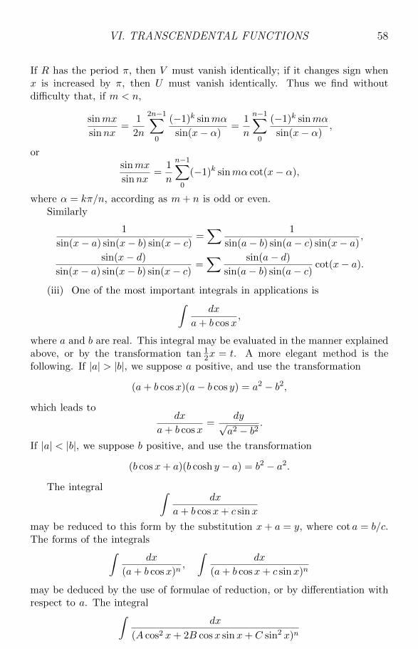
VI. TRANSCENDENTAL FUNCTIONS 58
If R has the period π, then V must vanish identically; if it changes sign whenx is increased by π, then U must vanish identically. Thus we find withoutdifficulty that, if m < n,
sinmx
sinnx=
1
2n
2n−1∑0
(−1)k sinmα
sin(x− α)=
1
n
n−1∑0
(−1)k sinmα
sin(x− α),
orsinmx
sinnx=
1
n
n−1∑0
(−1)k sinmα cot(x− α),
where α = kπ/n, according as m+ n is odd or even.Similarly
1
sin(x− a) sin(x− b) sin(x− c)=∑ 1
sin(a− b) sin(a− c) sin(x− a),
sin(x− d)
sin(x− a) sin(x− b) sin(x− c)=∑ sin(a− d)
sin(a− b) sin(a− c)cot(x− a).
(iii) One of the most important integrals in applications is∫dx
a+ b cosx,
where a and b are real. This integral may be evaluated in the manner explainedabove, or by the transformation tan 1
2x = t. A more elegant method is thefollowing. If |a| > |b|, we suppose a positive, and use the transformation
(a+ b cosx)(a− b cos y) = a2 − b2,
which leads todx
a+ b cosx=
dy√a2 − b2
.
If |a| < |b|, we suppose b positive, and use the transformation
(b cosx+ a)(b cosh y − a) = b2 − a2.
The integral ∫dx
a+ b cosx+ c sinx
may be reduced to this form by the substitution x+ a = y, where cot a = b/c.The forms of the integrals∫
dx
(a+ b cosx)n,
∫dx
(a+ b cosx+ c sinx)n
may be deduced by the use of formulae of reduction, or by differentiation withrespect to a. The integral∫
dx
(A cos2 x+ 2B cosx sinx+ C sin2 x)n

VI. TRANSCENDENTAL FUNCTIONS 59
is really of the same type, since
A cos2 x+ 2B cosx sinx+ C sin2 x = 12(A+ C) + 1
2(A− C) cos 2x+B sin 2x.
And similar methods may be applied to the corresponding integrals whichcontain hyperbolic functions, so that this type includes a large variety ofintegrals of common occurrence.
(iv) The same substitutions may of course be used when the subject ofintegration is an irrational function of cosx and sinx, though sometimes itis better to use the substitutions cosx = t, sinx = t, or tanx = t. Thus theintegral ∫
R(cosx, sinx,√X) dx,
whereX = (a, b, c, f, g, h G cosx, sinx, 1)2,
is reduced to an elliptic integral by the substitution tan 12x = t. The most
important integrals of this type are∫R(cosx, sinx) dx√
1− k2 sin2 x,
∫R(cosx, sinx) dx√α+ β cosx+ γ sinx
.
3. The integral ∫P (x, eax, ebx, . . . , ekx) dx,
where a, b, . . . , k are any numbers (commensurable or not), and P is apolynomial, is always an elementary function. For it is obvious that theintegral can be reduced to the sum of a finite number of integrals of the type∫
xpeAx dx;
and ∫xpeAx dx =
(∂
∂A
)p ∫eAx dx =
(∂
∂A
)p eAxA.
This type of integral includes a large variety of integrals, such as∫xm(cos px)µ(sin qx)ν dx,
∫xm(cosh px)µ(sinh qx)ν dx,∫
xme−αx(cos px)µ dx,
∫xme−αx(sin qx)ν dx,
(m, µ, ν, being positive integers) for which formulae of reduction are given intext-books on the integral calculus.
Such integrals as∫P (x, log x) dx,
∫P (x, arc sinx) dx, . . . ,
VI. TRANSCENDENTAL FUNCTIONS 60
where P is a polynomial, may be reduced to particular cases of the abovegeneral integral by the obvious substitutions
x = ey, x = sin y, . . . .
4. Except for the two classes of functions considered in the three precedingparagraphs, there are no really general classes of transcendental functionswhich we can always integrate in finite terms, although of course there areinnumerable particular forms which may be integrated by particular devices.There are however many classes of such integrals for which a systematicreduction theory may be given, analogous to the reduction theory for ellipticintegrals. Such a reduction theory endeavours in each case
(i) to split up any integral of the class under consideration into the sumof a number of parts of which some are elementary and the others not;
(ii) to reduce the number of the latter terms to the least possible;(iii) to prove that these terms are incapable of further reduction, and are
genuinely new and independent transcendents.As an example of this process we shall consider the integral∫
exR(x) dx
where R(x) is a rational function of x.∗ The theory of partial fractions enablesus to decompose this integral into the sum of a number of terms
A
∫ex
x− adx, . . . , Am
∫ex
(x− a)m+1dx, B
∫ex
x− bdx, . . . .
Since ∫ex
(x− a)m+1dx = − ex
m(x− a)m+
1
m
∫ex
(x− a)mdx,
the integral may be further reduced so as to contain only(i) a term
exS(x)
where S(x) is a rational function;(ii) a number of terms of the type
α
∫ex dx
x− a.
If all the constants α vanish, then the integral can be calculated in the finiteform exS(x). If they do not we can at any rate assert that the integral cannotbe calculated in this form†. For no such relation as
α
∫ex dx
x− a+ β
∫ex dx
x− b+ · · ·+ κ
∫ex dx
x− k= exT (x),
∗See Hermite, Cours d’analyse, pp. 352 et seq.†See the remarks at the end of this paragraph.

VI. TRANSCENDENTAL FUNCTIONS 61
where T is rational, can hold for all values of x. To see this it is only necessaryto put x = a+ h and to expand in ascending powers of h. Then
α
∫ex dx
x− a= αea
∫eh
hdh
= αea(log h+ h+ . . . ),
and no logarithm can occur in any of the other terms∗.Consider, for example, the integral∫
ex(
1− 1
x
)3
dx.
This is equal to
ex − 3
∫ex
xdx+ 3
∫ex
x2dx−
∫ex
x3dx,
and since
3
∫ex
x2dx = −3ex
x+ 3
∫ex
xdx,
and
−∫
ex
x3dx =
ex
2x2− 1
2
∫ex
x2dx =
ex
2x2+ex
2x− 1
2
∫ex
xdx,
we obtain finally∫ex(
1− 1
x
)3
dx = ex(
1− 7
2x+
1
2x2
)− 1
2
∫ex
xdx.
Similarly it will be found that∫ex(
1− 2
x
)2
dx = 2ex(
1
2− 2
x
),
this integral being an elementary function.Since ∫
ex
x− adx = ea
∫ey
ydy,
if x = y + a, all integrals of this kind may be made to depend on knownfunctions and on the single transcendent∫
ex
xdx,
which is usually denoted by Li ex and is of great importance in the theory ofnumbers. The question of course arises as to whether this integral is not itselfan elementary function.
∗It is not difficult to give a purely algebraical proof on the lines of iv., §2.

VI. TRANSCENDENTAL FUNCTIONS 62
Now Liouville∗ has proved the following theorem: ‘if y is any algebraicalfunction of x, and ∫
exy dx
is an elementary function, then∫exy dx = ex(α+ βy + · · ·+ λyn−1),
α, β, . . . , λ being rational functions of x and n the degree of the algebraicalequation which determines y as a function of x’.
Liouville’s proof rests on the same general principles as do those of thecorresponding theorems concerning the integral
∫y dx. It will be observed
that no logarithmic terms can occur, and that the theorem is therefore verysimilar to that which holds for
∫y dx in the simple case in which the integral
is algebraical. The argument which shows that no logarithmic terms occuris substantially the same as that which shows that, when they occur in theintegral of an algebraical function, they must occur linearly. In this casethe occurrence of the exponential factor precludes even this possibility, sincedifferentiation will not eliminate logarithms when they occur in the form
ex log f(x).
In particular, if y is a rational function, then the integral must be of theform
exR(x)
and this we have already seen to be impossible. Hence the ‘logarithm-integral’
Li ex =
∫ex
xdx =
∫ ex dy
log y
is really a new transcendent, which cannot be expressed in finite terms bymeans of elementary functions; and the same is true of all integrals of the type∫
exR(x) dx
which cannot be calculated in finite terms by means of the process of reductionsketched above.
The integrals ∫sinxR(x) dx,
∫cosxR(x) dx
∗‘Memoire sur l’integration d’une classe de fonctions transcendantes’, Journal furMathematik, vol. 13, 1835, pp. 93–118. Liouville shows how the integral, when of thisform, may always be calculated by elementary methods.

VI. TRANSCENDENTAL FUNCTIONS 63
may be treated in a similar manner. Either the integral is of the form
cosxR1(x) + sinxR2(x)
or it consists of a term of this kind together with a number of terms whichinvolve the transcendents ∫
cosx
xdx,
∫sinx
xdx,
which are called the cosine-integral and sine-integral of x, and denoted by Ci xand Si x. These transcendents are of course not fundamentally distinct fromthe logarithm-integral.
5. Liouville has gone further and shown that it is always possible todetermine whether the integral∫
(Pep +Qeq + · · ·+ Tet) dx,
where P , Q, . . . , T , p, q, . . . , t are algebraical functions, is an elementaryfunction, and to obtain the integral in case it is one∗. The most generaltheorem which has been proved in this region of mathematics, and which isalso due to Liouville, is the following.
‘If y, z, . . . are functions of x whose differential coefficients are algebraicalfunctions of x, y, z, . . . , and F denotes an algebraical function, and if∫
F (x, y, z, . . . ) dx
is an elementary function, then it is of the form
t+A log u+B log v + . . . ,
where t, u, v, . . . are algebraical functions of x, y, z, . . . . If the differentialcoefficients are rational in x, y, z, . . . , and F is rational, then t, u, v, . . . arerational in x, y, z, . . . .’
Thus for example the theorem applies to
F (x, ex, eex, log x, log log x, cosx, sinx),
since, if the various arguments of F are denoted by x, y, z, ξ, η, ζ, θ, we have
dy
dx= y,
dz
dx= yz,
dξ
dx=
1
x,
dη
dx=
1
xξ,
dζ
dx= −
√1− ζ2, dθ
dx=√
1− θ2.
The proof of the theorem does not involve ideas different in principle fromthose which have been employed continually throughout the preceding pages.
∗An interesting particular result is that the ‘error function’∫e−x
2
dx is not anelementary function.

VI. TRANSCENDENTAL FUNCTIONS 64
6. As a final example of the manner in which these ideas may be applied,we shall consider the following question:
‘in what circumstances is ∫R(x) log x dx,
where R is rational, an elementary function? ’In the first place the integral must be of the form
R0(x, log x) +A1 logR1(x, log x) +A2 logR2(x, log x) + . . . .
A general consideration of the form of the differential coefficient of thisexpression, in which log x must only occur linearly and multiplied by a rationalfunction, leads us to anticipate that (i) R0(x, log x) must be of the form
S(x)(log x)2 + T (x) log x+ U(x),
where S, T , and U are rational, and (ii) R1, R2, . . . must be rational functionsof x only; so that the integral can be expressed in the form
S(x)(log x)2 + T (x) log x+ U(x) +∑
Bk log(x− ak).
Differentiating, and comparing the result with the subject of integration,we obtain the equations
S′ = 0,2S
x+ T ′ = R,
T
x+ U ′ +
∑ Bkx− ak
= 0.
Hence S is a constant, say 12C, and
T =
∫ (R− C
x
)dx.
We can always determine by means of elementary operations, as in iv., §4,whether this integral is rational for any value of C or not. If not, then thegiven integral is not an elementary function. If T is rational, then we mustcalculate its value, and substitute it in the integral
U = −∫
T
x+∑ Bk
x− ak
dx = −
∫T
xdx−
∑Bk log(x− ak),
which must be rational for some value of the arbitrary constant implied in T .We can calculate the rational part of∫
T
xdx :
the transcendental part must be cancelled by the logarithmic terms∑Bk log(x− ak).

The necessary and sufficient condition that the original integral should bean elementary function is therefore that R should be of the form
C
x+
d
dxR1(x),
where C is a constant and R1 is rational. That the integral is in this case sucha function becomes obvious if we integrate by parts, for∫ (
C
x+R′1
)log x dx = 1
2C(log x)2 +R1 log x−∫R1
xdx.
In particular
(i)
∫log x
x− adx, (ii)
∫log x
(x− a)(x− b)dx,
are not elementary functions unless in (i) a = 0 and in (ii) b = a. If theintegral is elementary then the integration can always be carried out, with thesame reservation as was necessary in the case of rational functions.
It is evident that the problem considered in this paragraph is but one of awhole class of similar problems. The reader will find it instructive to formulateand consider such problems for himself.
7. It will be obvious by now that the number of classes of transcendentalfunctions whose integrals are always elementary is very small, and that suchintegrals as ∫
f(x, ex) dx,
∫f(x, log x) dx,∫
f(x, cosx, sinx) dx,
∫f(ex, cosx, sinx) dx,
. . . . . . . . . . . . . . . . . . . . . . ,
where f is algebraical, or even rational, are generally new transcendents. Thesenew transcendents, like the transcendents (such as the elliptic integrals) whicharise from the integration of algebraical functions, are in many cases of greatinterest and importance. They may often be expressed by means of infiniteseries or definite integrals, or their properties may be studied by means of theintegral expressions which define them. The very fact that such a functionis not an elementary function in so far enhances its importance. And whensuch functions have been introduced into analysis new problems of integrationarise in connection with them. We may enquire, for example, under whatcircumstances an elliptic integral or elliptic function, or a combination of suchfunctions with elementary functions, can be integrated in finite terms by meansof elementary and elliptic functions. But before we can be in a position torestate the fundamental problem of the Integral Calculus in any such moregeneral form, it is essential that we should have disposed of the particularproblem formulated in Section III.

APPENDIX I
BIBLIOGRAPHY
The following is a list of the memoirs by Abel, Liouville and Tschebyschef whichhave reference to the subject matter of this tract.
N. H. Abel
1. ‘Uber die Integration der Differential-Formelρ dx√R
, wenn R und ρ ganze
Funktionen sind’, Journal fur Mathematik, vol. 1, 1826, pp. 185–221 (Œuvres,vol. 1, pp. 104–144).
2. ‘Precis d’une theorie des fonctions elliptiques’, Journal fur Mathematik, vol. 4,1829, pp. 236–277, 309–348 (Œuvres, vol. 1, pp. 518–617).
3. ‘Theorie des transcendantes elliptiques’, Œuvres, vol. 2, pp. 87–188.
J. Liouville
1. ‘Memoire sur la classification des transcendantes, et sur l’impossibilite d’exprimerles racines de certaines equations en fonction finie explicite des coefficients’,Journal de mathematiques, ser. 1, vol. 2, 1837, pp. 56–104.
2. ‘Nouvelles recherches sur la determination des integrales dont la valeur estalgebrique’, ibid., vol. 3, 1838, pp. 20–24 (previously published in the ComptesRendus, 28 Aug. 1837).
3. ‘Suite du memoire sur la classification des transcendantes, et sur l’impossibilited’exprimer les racines de certaines equations en fonction finie explicite descoefficients’, ibid., pp. 523–546.
4. ‘Note sur les transcendantes elliptiques considerees comme fonctions de leurmodule’, ibid., vol. 5, 1840, pp. 34–37.
5. ‘Memoire sur les transcendantes elliptiques considerees comme fonctions de leurmodule’, ibid., pp. 441–464.
6. ‘Premier memoire sur la determination des integrales dont la valeur est algebrique’,Journal de l’Ecole Polytechnique, vol. 14, cahier 22, 1833, pp. 124–148 (alsopublished in the Memoires presentes par divers savants a l’Academie desSciences, vol. 5, 1838, pp. 76–151).
7. ‘Second memoire sur la determination des integrales dont la valeur est algebrique’,ibid., pp. 149–193 (also published as above).
8. ‘Memoire sur les transcendantes elliptiques considerees comme fonctions de leuramplitude’, ibid., cahier 23, 1834, pp. 37–83.
9. ‘Memoire sur l’integration d’une classe de fonctions transcendantes’, Journal furMathematik, vol. 13, 1835, pp. 93–118.
P. Tschebyschef
1. ‘Sur l’integration des differentielles irrationnelles’, Journal de mathematiques,ser. 1, vol. 18, 1853, pp. 87–111 (Œuvres, vol. 1, pp. 147–168).
2. ‘Sur l’integration des differentielles qui contiennent une racine carree d’unepolynome du troisieme ou du quatrieme degre’, ibid., ser. 2, vol. 2, 1857,pp. 1–42 (Œuvres, vol. 1, pp. 171–200; also published in the Memoires de

l’Academie Imperiale des Sciences de St-Petersbourg, ser. 6, vol. 6, 1857,pp. 203–232).
3. ‘Sur l’integration de la differentiellex+A√
x4 + αx3 + βx2 + γx+ δdx’, ibid., ser. 2,
vol. 9, 1864, pp. 225–241 (Œuvres, vol. 1, pp. 517–530; previously publishedin the Bulletin de l’Academie Imperiale des Sciences de St-Petersbourg, vol. 3,1861, pp. 1–12).
4. ‘Sur l’integration des differentielles irrationnelles’, ibid., pp. 242–246 (Œuvres,vol. 1, pp. 511–514; previously published in the Comptes Rendus, 9 July 1860).
5. ‘Sur l’integration des differentielles qui contiennent une racine cubique’ (Œuvres,vol. 1, pp. 563–608; previously published only in Russian).
Other memoirs which may be consulted are:
A. Clebsch
‘Uber diejenigen Curven, deren Coordinaten sich als elliptische Functioneneines Parameters darstellen lassen’, Journal fur Mathematik, vol. 64, 1865,pp. 210–270.
J. Dolbnia
‘Sur les integrales pseudo-elliptiques d’Abel’, Journal de mathematiques, ser. 4,vol. 6, 1890, pp. 293–311.
Sir A. G. Greenhill
‘Pseudo-elliptic integrals and their dynamical applications’, Proc. London Math.Soc., ser. 1, vol. 25, 1894, pp. 195–304.
G. H. Hardy
‘Properties of logarithmico-exponential functions’, Proc. London Math. Soc., ser. 2,vol. 10, 1910, pp. 54–90.
L. Konigsberger
‘Bemerkungen zu Liouville’s Classificirung der Transcendenten’, MathematischeAnnalen, vol. 28, 1886, pp. 483–492.
L. Raffy
‘Sur les quadratures algebriques et logarithmiques’, Annales de l’Ecole Normale,ser. 3, vol. 2, 1885, pp. 185–206.
K. Weierstrass
‘Uber die Integration algebraischer Differentiale vermittelst Logarithmen’,Monatsberichte der Akademie der Wissenschaften zu Berlin, 1857, pp. 148–157(Werke, vol. 1, pp. 227–232).
G. Zolotareff
‘Sur la methode d’integration de M. Tschebyschef’, Journal de mathematiques,ser. 2, vol. 19, 1874, pp. 161–188.
Further information concerning pseudo-elliptic integrals, and degenerate cases of
Abelian integrals generally, will be found in a number of short notes by Dolbnia,
Kapteyn and Ptaszycki in the Bulletin des sciences mathematiques, and by Goursat,
Gunther, Picard, Poincare, and Raffy in the Bulletin de la Societe Mathematique de
France, in Legendre’s Traite des functions elliptiques (vol. 1, ch. 26), in Halphen’s
Traite des fonctions elliptiques (vol. 2, ch. 14), and in Enneper’s Elliptische
Funktionen. The literature concerning the general theory of algebraical functions and
their integrals is too extensive to be summarised here: the reader may be referred
to Appell and Goursat’s Theorie des fonctions algebriques, and Wirtinger’s article
Algebraische Funktionen und ihre Integrale in the Encyclopadie der Mathematischen
Wissenschaften, ii B 2.

APPENDIX II
ON ABEL’S PROOF OF THE THEOREM OF V., §11
Abel’s proof (Œuvres, vol. 1, p. 545) is as follows∗:We have
ψ(x, u) = 0, (1)
where ψ is an irreducible polynomial of degree m in u. If we make use of theequation f(x, y) = 0, we can introduce y into this equation, and write it in theform
φ(x, y, u) = 0, (2)
where φ is a polynomial in the three variables x, y, and u†; and we cansuppose φ, like ψ, of degree m in u and irreducible, that is to say not divisibleby any polynomial of the same form which is not a constant multiple of φ oritself a constant.
From f = 0, φ = 0 we deduce
∂f
∂x+∂f
∂y
dy
dx= 0,
∂φ
∂x+∂φ
∂y
dy
dx+∂φ
∂u
du
dx= 0;
and, eliminatingdy
dx, we obtain an equation of the form
du
dx=λ(x, y, u)
µ(x, y, u),
where λ and µ are polynomials in x, y, and u. And in order that u should bean integral of y it is necessary and sufficient that
λ− yµ = 0. (3)
Abel now applies Lemma (2) of §11, or rather its analogue for polynomialsin u whose coefficients are polynomials in x and y, to the two polynomials φand λ− yµ, and infers that all the roots u, u′, . . . of φ = 0 satisfy (3). Fromthis he deduces that u, u′, . . . are all integrals of y, and so that
u+ u′ + . . .
m+ 1(4)
is an integral of y. As (4) is a symmetric function of the roots of (2), it is arational function of x and y, whence his conclusion follows‡.
∗The theorem with which Abel is engaged is a very much more general theorem.†‘Or, au lieu de supposer ces coefficiens rationnels en x, nous les supposerons
rationnels en x, y; car cette supposition permise simplifiera beaucoup le raisonnement ’.‡Bertrand (Calcul integral, ch. 5) replaces the last step in Abel’s argument by the
observation that if u and u′ are both integrals of y then u− u′ is constant (cf. p. 39,bottom). It follows that the degree of the equation which defines u can be decreased,which contradicts the hypothesis that it is irreducible.

It will be observed that the hypothesis that (2) does actually involve yis essential, if we are to avoid the absurd conclusion that u is necessarily arational function of x only. On the other hand it is not obvious how thepresence of y in φ affects the other steps in the argument.
The crucial inference is that which asserts that because the equations φ = 0and λ− yµ = 0, considered as equations in u, have a root in common, and φ isirreducible, therefore λ− yµ is divisible by φ. This inference is invalid.
We could only apply the lemma in this way if the equation (3) weresatisfied by one of the roots of (2) identically, that is to say for all values ofx and y. But this is not the case. The equations are satisfied by the samevalue of u only when x and y are connected by the equation (1).
Suppose, for example, that
y =1√
1 + x, u = 2
√1 + x.
Then we may take
f = (1 + x)y2 − 1,
ψ = u2 − 4(1 + x),
and
φ = uy − 2.
Differentiating the equations f = 0 and φ = 0, and eliminatingdy
dx, we find
du
dx=
u
2(1 + x)=λ
µ.
Thusφ = uy − 2, λ− yµ = u− 2y(1 + x);
and these polynomials have a common factor only in virtue of the equationf = 0.

PUBLISHED BYTHE SYNDICS OF THE CAMBRIDGE UNIVERSITY PRESS
Bentley House, 200 Euston Road, London, N.W.1American Branch: 32 East 57th Street, New York 10022, N.Y.
PRINTED IN GREAT BRITAIN

End of the Project Gutenberg EBook of The Integration of Functions of aSingle Variable, by G. H. Hardy
*** END OF THIS PROJECT GUTENBERG EBOOK INTEGRATION OF FUNCTIONS OF ONE VARIABLE ***
***** This file should be named 38993-t.tex or 38993-t.zip *****This and all associated files of various formats will be found in:
http://www.gutenberg.org/3/8/9/9/38993/
Produced by Brenda Lewis, Anna Hall and the OnlineDistributed Proofreading Team at http://www.pgdp.net (Thisfile was produced from images generously made availableby The Internet Archive/American Libraries.)
Updated editions will replace the previous one--the old editionswill be renamed.
Creating the works from public domain print editions means that noone owns a United States copyright in these works, so the Foundation(and you!) can copy and distribute it in the United States withoutpermission and without paying copyright royalties. Special rules,set forth in the General Terms of Use part of this license, apply tocopying and distributing Project Gutenberg-tm electronic works toprotect the PROJECT GUTENBERG-tm concept and trademark. ProjectGutenberg is a registered trademark, and may not be used if youcharge for the eBooks, unless you receive specific permission. If youdo not charge anything for copies of this eBook, complying with therules is very easy. You may use this eBook for nearly any purposesuch as creation of derivative works, reports, performances andresearch. They may be modified and printed and given away--you may dopractically ANYTHING with public domain eBooks. Redistribution issubject to the trademark license, especially commercialredistribution.
*** START: FULL LICENSE ***
THE FULL PROJECT GUTENBERG LICENSEPLEASE READ THIS BEFORE YOU DISTRIBUTE OR USE THIS WORK
To protect the Project Gutenberg-tm mission of promoting the freedistribution of electronic works, by using or distributing this work(or any other work associated in any way with the phrase "ProjectGutenberg"), you agree to comply with all the terms of the Full ProjectGutenberg-tm License available with this file or online atwww.gutenberg.org/license.
Section 1. General Terms of Use and Redistributing Project Gutenberg-tmelectronic works
1.A. By reading or using any part of this Project Gutenberg-tmelectronic work, you indicate that you have read, understand, agree toand accept all the terms of this license and intellectual property(trademark/copyright) agreement. If you do not agree to abide by allthe terms of this agreement, you must cease using and return or destroyall copies of Project Gutenberg-tm electronic works in your possession.If you paid a fee for obtaining a copy of or access to a ProjectGutenberg-tm electronic work and you do not agree to be bound by theterms of this agreement, you may obtain a refund from the person orentity to whom you paid the fee as set forth in paragraph 1.E.8.
1.B. "Project Gutenberg" is a registered trademark. It may only beused on or associated in any way with an electronic work by people whoagree to be bound by the terms of this agreement. There are a few
things that you can do with most Project Gutenberg-tm electronic workseven without complying with the full terms of this agreement. Seeparagraph 1.C below. There are a lot of things you can do with ProjectGutenberg-tm electronic works if you follow the terms of this agreementand help preserve free future access to Project Gutenberg-tm electronicworks. See paragraph 1.E below.
1.C. The Project Gutenberg Literary Archive Foundation ("the Foundation"or PGLAF), owns a compilation copyright in the collection of ProjectGutenberg-tm electronic works. Nearly all the individual works in thecollection are in the public domain in the United States. If anindividual work is in the public domain in the United States and you arelocated in the United States, we do not claim a right to prevent you fromcopying, distributing, performing, displaying or creating derivativeworks based on the work as long as all references to Project Gutenbergare removed. Of course, we hope that you will support the ProjectGutenberg-tm mission of promoting free access to electronic works byfreely sharing Project Gutenberg-tm works in compliance with the terms ofthis agreement for keeping the Project Gutenberg-tm name associated withthe work. You can easily comply with the terms of this agreement bykeeping this work in the same format with its attached full ProjectGutenberg-tm License when you share it without charge with others.
1.D. The copyright laws of the place where you are located also governwhat you can do with this work. Copyright laws in most countries are ina constant state of change. If you are outside the United States, checkthe laws of your country in addition to the terms of this agreementbefore downloading, copying, displaying, performing, distributing orcreating derivative works based on this work or any other ProjectGutenberg-tm work. The Foundation makes no representations concerningthe copyright status of any work in any country outside the UnitedStates.
1.E. Unless you have removed all references to Project Gutenberg:
1.E.1. The following sentence, with active links to, or other immediateaccess to, the full Project Gutenberg-tm License must appear prominentlywhenever any copy of a Project Gutenberg-tm work (any work on which thephrase "Project Gutenberg" appears, or with which the phrase "ProjectGutenberg" is associated) is accessed, displayed, performed, viewed,copied or distributed:
This eBook is for the use of anyone anywhere at no cost and withalmost no restrictions whatsoever. You may copy it, give it away orre-use it under the terms of the Project Gutenberg License includedwith this eBook or online at www.gutenberg.org
1.E.2. If an individual Project Gutenberg-tm electronic work is derivedfrom the public domain (does not contain a notice indicating that it isposted with permission of the copyright holder), the work can be copiedand distributed to anyone in the United States without paying any feesor charges. If you are redistributing or providing access to a workwith the phrase "Project Gutenberg" associated with or appearing on thework, you must comply either with the requirements of paragraphs 1.E.1through 1.E.7 or obtain permission for the use of the work and theProject Gutenberg-tm trademark as set forth in paragraphs 1.E.8 or1.E.9.
1.E.3. If an individual Project Gutenberg-tm electronic work is postedwith the permission of the copyright holder, your use and distributionmust comply with both paragraphs 1.E.1 through 1.E.7 and any additionalterms imposed by the copyright holder. Additional terms will be linkedto the Project Gutenberg-tm License for all works posted with thepermission of the copyright holder found at the beginning of this work.
1.E.4. Do not unlink or detach or remove the full Project Gutenberg-tmLicense terms from this work, or any files containing a part of this

work or any other work associated with Project Gutenberg-tm.
1.E.5. Do not copy, display, perform, distribute or redistribute thiselectronic work, or any part of this electronic work, withoutprominently displaying the sentence set forth in paragraph 1.E.1 withactive links or immediate access to the full terms of the ProjectGutenberg-tm License.
1.E.6. You may convert to and distribute this work in any binary,compressed, marked up, nonproprietary or proprietary form, including anyword processing or hypertext form. However, if you provide access to ordistribute copies of a Project Gutenberg-tm work in a format other than"Plain Vanilla ASCII" or other format used in the official versionposted on the official Project Gutenberg-tm web site (www.gutenberg.org),you must, at no additional cost, fee or expense to the user, provide acopy, a means of exporting a copy, or a means of obtaining a copy uponrequest, of the work in its original "Plain Vanilla ASCII" or otherform. Any alternate format must include the full Project Gutenberg-tmLicense as specified in paragraph 1.E.1.
1.E.7. Do not charge a fee for access to, viewing, displaying,performing, copying or distributing any Project Gutenberg-tm worksunless you comply with paragraph 1.E.8 or 1.E.9.
1.E.8. You may charge a reasonable fee for copies of or providingaccess to or distributing Project Gutenberg-tm electronic works providedthat
- You pay a royalty fee of 20% of the gross profits you derive fromthe use of Project Gutenberg-tm works calculated using the methodyou already use to calculate your applicable taxes. The fee isowed to the owner of the Project Gutenberg-tm trademark, but hehas agreed to donate royalties under this paragraph to theProject Gutenberg Literary Archive Foundation. Royalty paymentsmust be paid within 60 days following each date on which youprepare (or are legally required to prepare) your periodic taxreturns. Royalty payments should be clearly marked as such andsent to the Project Gutenberg Literary Archive Foundation at theaddress specified in Section 4, "Information about donations tothe Project Gutenberg Literary Archive Foundation."
- You provide a full refund of any money paid by a user who notifiesyou in writing (or by e-mail) within 30 days of receipt that s/hedoes not agree to the terms of the full Project Gutenberg-tmLicense. You must require such a user to return ordestroy all copies of the works possessed in a physical mediumand discontinue all use of and all access to other copies ofProject Gutenberg-tm works.
- You provide, in accordance with paragraph 1.F.3, a full refund of anymoney paid for a work or a replacement copy, if a defect in theelectronic work is discovered and reported to you within 90 daysof receipt of the work.
- You comply with all other terms of this agreement for freedistribution of Project Gutenberg-tm works.
1.E.9. If you wish to charge a fee or distribute a Project Gutenberg-tmelectronic work or group of works on different terms than are setforth in this agreement, you must obtain permission in writing fromboth the Project Gutenberg Literary Archive Foundation and MichaelHart, the owner of the Project Gutenberg-tm trademark. Contact theFoundation as set forth in Section 3 below.
1.F.
1.F.1. Project Gutenberg volunteers and employees expend considerable

effort to identify, do copyright research on, transcribe and proofreadpublic domain works in creating the Project Gutenberg-tmcollection. Despite these efforts, Project Gutenberg-tm electronicworks, and the medium on which they may be stored, may contain"Defects," such as, but not limited to, incomplete, inaccurate orcorrupt data, transcription errors, a copyright or other intellectualproperty infringement, a defective or damaged disk or other medium, acomputer virus, or computer codes that damage or cannot be read byyour equipment.
1.F.2. LIMITED WARRANTY, DISCLAIMER OF DAMAGES - Except for the "Rightof Replacement or Refund" described in paragraph 1.F.3, the ProjectGutenberg Literary Archive Foundation, the owner of the ProjectGutenberg-tm trademark, and any other party distributing a ProjectGutenberg-tm electronic work under this agreement, disclaim allliability to you for damages, costs and expenses, including legalfees. YOU AGREE THAT YOU HAVE NO REMEDIES FOR NEGLIGENCE, STRICTLIABILITY, BREACH OF WARRANTY OR BREACH OF CONTRACT EXCEPT THOSEPROVIDED IN PARAGRAPH 1.F.3. YOU AGREE THAT THE FOUNDATION, THETRADEMARK OWNER, AND ANY DISTRIBUTOR UNDER THIS AGREEMENT WILL NOT BELIABLE TO YOU FOR ACTUAL, DIRECT, INDIRECT, CONSEQUENTIAL, PUNITIVE ORINCIDENTAL DAMAGES EVEN IF YOU GIVE NOTICE OF THE POSSIBILITY OF SUCHDAMAGE.
1.F.3. LIMITED RIGHT OF REPLACEMENT OR REFUND - If you discover adefect in this electronic work within 90 days of receiving it, you canreceive a refund of the money (if any) you paid for it by sending awritten explanation to the person you received the work from. If youreceived the work on a physical medium, you must return the medium withyour written explanation. The person or entity that provided you withthe defective work may elect to provide a replacement copy in lieu of arefund. If you received the work electronically, the person or entityproviding it to you may choose to give you a second opportunity toreceive the work electronically in lieu of a refund. If the second copyis also defective, you may demand a refund in writing without furtheropportunities to fix the problem.
1.F.4. Except for the limited right of replacement or refund set forthin paragraph 1.F.3, this work is provided to you ’AS-IS’, WITH NO OTHERWARRANTIES OF ANY KIND, EXPRESS OR IMPLIED, INCLUDING BUT NOT LIMITED TOWARRANTIES OF MERCHANTABILITY OR FITNESS FOR ANY PURPOSE.
1.F.5. Some states do not allow disclaimers of certain impliedwarranties or the exclusion or limitation of certain types of damages.If any disclaimer or limitation set forth in this agreement violates thelaw of the state applicable to this agreement, the agreement shall beinterpreted to make the maximum disclaimer or limitation permitted bythe applicable state law. The invalidity or unenforceability of anyprovision of this agreement shall not void the remaining provisions.
1.F.6. INDEMNITY - You agree to indemnify and hold the Foundation, thetrademark owner, any agent or employee of the Foundation, anyoneproviding copies of Project Gutenberg-tm electronic works in accordancewith this agreement, and any volunteers associated with the production,promotion and distribution of Project Gutenberg-tm electronic works,harmless from all liability, costs and expenses, including legal fees,that arise directly or indirectly from any of the following which you door cause to occur: (a) distribution of this or any Project Gutenberg-tmwork, (b) alteration, modification, or additions or deletions to anyProject Gutenberg-tm work, and (c) any Defect you cause.
Section 2. Information about the Mission of Project Gutenberg-tm
Project Gutenberg-tm is synonymous with the free distribution ofelectronic works in formats readable by the widest variety of computersincluding obsolete, old, middle-aged and new computers. It exists
because of the efforts of hundreds of volunteers and donations frompeople in all walks of life.
Volunteers and financial support to provide volunteers with theassistance they need are critical to reaching Project Gutenberg-tm’sgoals and ensuring that the Project Gutenberg-tm collection willremain freely available for generations to come. In 2001, the ProjectGutenberg Literary Archive Foundation was created to provide a secureand permanent future for Project Gutenberg-tm and future generations.To learn more about the Project Gutenberg Literary Archive Foundationand how your efforts and donations can help, see Sections 3 and 4and the Foundation information page at www.gutenberg.org
Section 3. Information about the Project Gutenberg Literary ArchiveFoundation
The Project Gutenberg Literary Archive Foundation is a non profit501(c)(3) educational corporation organized under the laws of thestate of Mississippi and granted tax exempt status by the InternalRevenue Service. The Foundation’s EIN or federal tax identificationnumber is 64-6221541. Contributions to the Project GutenbergLiterary Archive Foundation are tax deductible to the full extentpermitted by U.S. federal laws and your state’s laws.
The Foundation’s principal office is located at 4557 Melan Dr. S.Fairbanks, AK, 99712., but its volunteers and employees are scatteredthroughout numerous locations. Its business office is located at 809North 1500 West, Salt Lake City, UT 84116, (801) 596-1887. Emailcontact links and up to date contact information can be found at theFoundation’s web site and official page at www.gutenberg.org/contact
For additional contact information:Dr. Gregory B. NewbyChief Executive and [email protected]
Section 4. Information about Donations to the Project GutenbergLiterary Archive Foundation
Project Gutenberg-tm depends upon and cannot survive without widespread public support and donations to carry out its mission ofincreasing the number of public domain and licensed works that can befreely distributed in machine readable form accessible by the widestarray of equipment including outdated equipment. Many small donations($1 to $5,000) are particularly important to maintaining tax exemptstatus with the IRS.
The Foundation is committed to complying with the laws regulatingcharities and charitable donations in all 50 states of the UnitedStates. Compliance requirements are not uniform and it takes aconsiderable effort, much paperwork and many fees to meet and keep upwith these requirements. We do not solicit donations in locationswhere we have not received written confirmation of compliance. ToSEND DONATIONS or determine the status of compliance for anyparticular state visit www.gutenberg.org/donate
While we cannot and do not solicit contributions from states where wehave not met the solicitation requirements, we know of no prohibitionagainst accepting unsolicited donations from donors in such states whoapproach us with offers to donate.
International donations are gratefully accepted, but we cannot makeany statements concerning tax treatment of donations received fromoutside the United States. U.S. laws alone swamp our small staff.
Please check the Project Gutenberg Web pages for current donation

methods and addresses. Donations are accepted in a number of otherways including checks, online payments and credit card donations.To donate, please visit: www.gutenberg.org/donate
Section 5. General Information About Project Gutenberg-tm electronicworks.
Professor Michael S. Hart was the originator of the Project Gutenberg-tmconcept of a library of electronic works that could be freely sharedwith anyone. For forty years, he produced and distributed ProjectGutenberg-tm eBooks with only a loose network of volunteer support.
Project Gutenberg-tm eBooks are often created from several printededitions, all of which are confirmed as Public Domain in the U.S.unless a copyright notice is included. Thus, we do not necessarilykeep eBooks in compliance with any particular paper edition.
Most people start at our Web site which has the main PG search facility:
www.gutenberg.org
This Web site includes information about Project Gutenberg-tm,including how to make donations to the Project Gutenberg LiteraryArchive Foundation, how to help produce our new eBooks, and how tosubscribe to our email newsletter to hear about new eBooks.