
The price specie °ow mechanism - Universitetet i Oslo€™s specie-°ow theory The country has a...
24
The price specie flow mechanism Slides for Chapter 6.6 of Open Economy Macroeconomics Asbjørn Rødseth University of Oslo 1st April 2008 Asbjørn Rødseth (University of Oslo) The price specie flow mechanism 1st April 2008 1 / 20
Transcript of The price specie °ow mechanism - Universitetet i Oslo€™s specie-°ow theory The country has a...

The price specie flow mechanismSlides for Chapter 6.6 of Open Economy Macroeconomics
Asbjørn Rødseth
University of Oslo
1st April 2008
Asbjørn Rødseth (University of Oslo) The price specie flow mechanism 1st April 2008 1 / 20

Hume’s specie-flow theory
The country has a trade deficit
→ Gold and silver flows out
→ Wealth declines gradually
→ Domestic demand falls
→ Prices of home goods (and wages) decline
→ Imports go down, exports up
→ Trade balance improves until deficit is eliminated
Asbjørn Rødseth (University of Oslo) The price specie flow mechanism 1st April 2008 2 / 20

Some assumptions
Home and foreign goods
Prices determined by wage cost (plus mark-up)
Fixed exchange rate, no change expected
Fixed interest rate, either
1 perfect capital mobility and credible exchange rate, or2 low capital mobility, interest rate set independently
Government budget balanced
No investment
No imported inflation
Asbjørn Rødseth (University of Oslo) The price specie flow mechanism 1st April 2008 3 / 20

The consumption function
C = C (Yp, Wp, ρ, ρ∗) 0 < CY < 1, CW > 0
In our case
Wp = −EF∗P
−Wg = −W ′∗ −Wg
W ′∗ = value of foreign debt measured in home goods
Yp = Y − i∗EF∗P
− G = Y + i∗Wp + i∗Wg − G
Savings: Sp = Yp − C
Assumption:dSp
dWp= i∗(1− CY )− CW < 0
Asbjørn Rødseth (University of Oslo) The price specie flow mechanism 1st April 2008 4 / 20
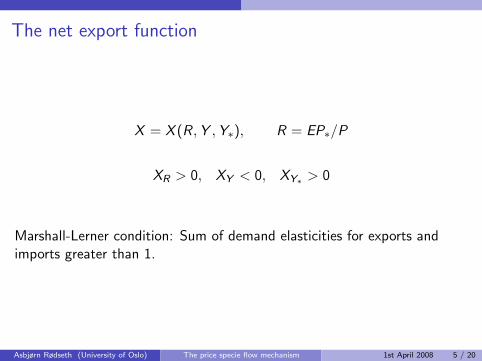
The net export function
X = X (R, Y , Y∗), R = EP∗/P
XR > 0, XY < 0, XY∗ > 0
Marshall-Lerner condition: Sum of demand elasticities for exports andimports greater than 1.
Asbjørn Rødseth (University of Oslo) The price specie flow mechanism 1st April 2008 5 / 20

The modelIS-curve:
Y = C
(Y − i∗
EF∗P
− G ,−EF∗P
−Wg , i , i∗
)+G +X
(EP∗P
, Y , Y∗
)(1)
Phillips-curve:P = Pγ(Y − Y ) (2)
Accumulation of foreign debt:
F∗ = i∗F∗ − P
EX
(EP∗P
, Y , Y∗
)(3)
Endogenous variables: Y , P and F∗
Initial conditions: P(0) = P0, F∗(0) = F∗0
Wg (0) = (−M0 − B0 + E (0)Fg0)/P0
Asbjørn Rødseth (University of Oslo) The price specie flow mechanism 1st April 2008 6 / 20

The temporary equilibrium
Y = C (Y − i∗EF∗P
− G ,−EF∗P
−Wg , i , i∗) + G + X (EP∗P
, Y , Y∗)
IS-equation determines Y given P and F∗ .Solution:
Y = Y (P ,F∗, x), x = (i∗, P∗,Y∗,G , i , E , Wg ) (4)
Increased foreign debt, F∗, reduces consumption demand and output
∂Y
∂F∗=
(−i∗CY − CW )E/P
1− CY − XY< 0 (5)
Asbjørn Rødseth (University of Oslo) The price specie flow mechanism 1st April 2008 7 / 20

Temporary equilibrium: Effect of the price level on output
Wealth effect. P ↑→ Reduced real value of F∗. Aggregate demand upif F∗ > 0, down if F∗ < 0
Real exchange rate effect. Demand shifts away from home goods.Aggregate demand down.
Total effect. Always negative for creditor country, may be positive forcountries with large debt.
∂Y
∂P=
(i∗CY + CW )W ′∗ − XRR
1− CY − XY
1
P(6)
Our assumption: ∂Y /∂P < 0.
Asbjørn Rødseth (University of Oslo) The price specie flow mechanism 1st April 2008 8 / 20
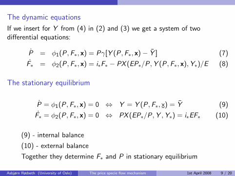
The dynamic equations
If we insert for Y from (4) in (2) and (3) we get a system of twodifferential equations:
P = φ1(P, F∗, x) = Pγ[Y (P, F∗, x)− Y ] (7)
F∗ = φ2(P, F∗, x) = i∗F∗ − PX (EP∗/P, Y (P,F∗, x),Y∗)/E (8)
The stationary equilibrium
P = φ1(P ,F∗, x) = 0 ⇔ Y = Y (P ,F∗, x¯) = Y (9)
F∗ = φ2(P ,F∗, x) = 0 ⇔ PX (EP∗/P, Y , Y∗) = i∗EF∗ (10)
(9) - internal balance
(10) - external balance
Together they determine F∗ and P in stationary equilibrium
Asbjørn Rødseth (University of Oslo) The price specie flow mechanism 1st April 2008 9 / 20

The stationary (long run) equilibrium
Since a stationary equilibrium is also a temporary equilibrium:
C (Y − i∗W ′∗ − G ,−W ′
∗ −Wg , i , i∗) + G + X (R, Y , Y∗) = Y (11)
With Y = Y external balance requires
i∗W ′∗ = X (R, Y ,Y∗) (12)
Use (12) to eliminate X from (11):
C (Y − i∗W ′∗ − G ,−W ′
∗ −Wg , i , i∗) + G = Y − i∗W ′∗ (13)
(13) determines W ′∗(12) then determines R
Asbjørn Rødseth (University of Oslo) The price specie flow mechanism 1st April 2008 10 / 20

Long run equilibrium
Solution is recursive
Y determined by supply (capacity)
W ′∗ determined by savings behavior
R determined by demand for exports and imports
P determined by exchange rate
Implicitly: Wage level has to be low enough that a sufficient share of worlddemand is directed towards home goods.
Asbjørn Rødseth (University of Oslo) The price specie flow mechanism 1st April 2008 11 / 20
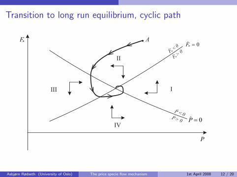
Transition to long run equilibrium, cyclic path
Asbjørn Rødseth (University of Oslo) The price specie flow mechanism 1st April 2008 12 / 20
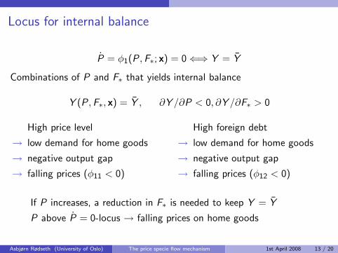
Locus for internal balance
P = φ1(P, F∗; x) = 0 ⇐⇒ Y = Y
Combinations of P and F∗ that yields internal balance
Y (P, F∗, x) = Y , ∂Y /∂P < 0, ∂Y /∂F∗ > 0
High price level
→ low demand for home goods
→ negative output gap
→ falling prices (φ11 < 0)
High foreign debt
→ low demand for home goods
→ negative output gap
→ falling prices (φ12 < 0)
If P increases, a reduction in F∗ is needed to keep Y = Y
P above P = 0-locus → falling prices on home goods
Asbjørn Rødseth (University of Oslo) The price specie flow mechanism 1st April 2008 13 / 20

Locus for external balance
Combinations of P and F∗ that yields external balance are defined by:
F∗ = φ2(P,F∗; x) = 0
X (EP∗/P, Y (P,F∗, x),Y∗)− i∗EF∗/P = 0
Increase in F∗Two opposing effects on the current account:
more interest payments on foreign debt
improved trade balance since output is down
Our assumption:
Trade effect dominates, current account improved(φ22 < 0)
Asbjørn Rødseth (University of Oslo) The price specie flow mechanism 1st April 2008 14 / 20

Locus for external balance
X (EP∗/P, Y (P,F∗, x),Y∗)− i∗EF∗/P = 0
Increase in P
Effects through two channels:
1. A real appreciation, which worsen the current account
2. A change in the real value of the foreign debt.
The sign of the second effect depends on the sign of F∗:If F∗ > 0, P ↑ works like a reduction in F∗, assumed above to worsenthe current account.
I F∗ < 0, P ↑ works like an increase in F∗, improving the currentaccount
Our assumption:
Real exchange rate effects dominate, current account worsens(φ21 > 0)
Asbjørn Rødseth (University of Oslo) The price specie flow mechanism 1st April 2008 14 / 20

External balance, summing up
Our assumptions:
An increase in F∗ improves current account (φ22 < 0)
An increase in P worsens current account (φ21 > 0)
Locus for external balance slopes upward: If P increases, a higher F∗ isrequired to keep current account balanced.
If F∗ is above the locus for external balance, F∗ is declining.
Asbjørn Rødseth (University of Oslo) The price specie flow mechanism 1st April 2008 15 / 20

The transition to long run equilibrium
Phase II
Output below capacity
Prices falling
Current account surplus
Foreign debt declining
Until internal balance is reached
Asbjørn Rødseth (University of Oslo) The price specie flow mechanism 1st April 2008 16 / 20

The transition to long run equilibrium
Phase III
Output above capacity
Prices increasing
Current account surplus
Foreign debt declining
Until external balance is reached
Asbjørn Rødseth (University of Oslo) The price specie flow mechanism 1st April 2008 16 / 20
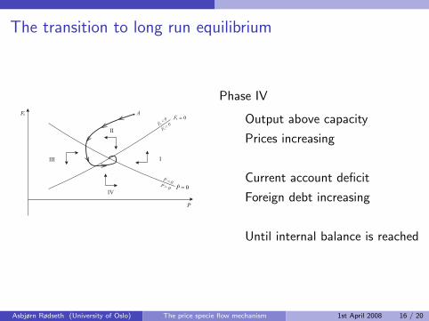
The transition to long run equilibrium
Phase IV
Output above capacity
Prices increasing
Current account deficit
Foreign debt increasing
Until internal balance is reached
Asbjørn Rødseth (University of Oslo) The price specie flow mechanism 1st April 2008 16 / 20
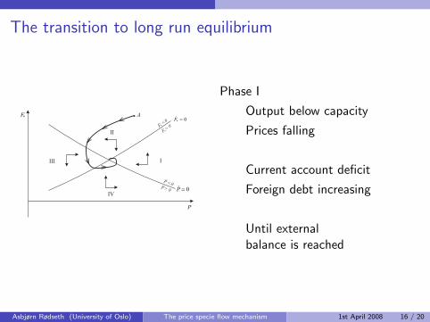
The transition to long run equilibrium
Phase I
Output below capacity
Prices falling
Current account deficit
Foreign debt increasing
Until externalbalance is reached
Asbjørn Rødseth (University of Oslo) The price specie flow mechanism 1st April 2008 16 / 20

Stability conditions
Stability cannot be proved by looking at graphs aloneJacobian matrix
A =
[φ11 φ12
φ21 φ22
]
Necessary and sufficient conditions for stability
tr(A) = φ11 + φ22 < 0
and|A| = φ11φ22 − φ12φ21 > 0
Our assumptions ensure that both conditions are satisfied, but they arestricter than necessary.Can be shown:
|A| > 0 ⇐⇒ i∗(1− CY )− CW < 0
Or: Increased wealth must lead to reduced savings.
Asbjørn Rødseth (University of Oslo) The price specie flow mechanism 1st April 2008 17 / 20

The transition to long run equilibrium, non-cyclic path
Asbjørn Rødseth (University of Oslo) The price specie flow mechanism 1st April 2008 18 / 20

The effect of easier access to credit
Positive shift in domestic demand
Internal balance requires higherprices
External balance requires lower prices
First boom, then recessionFirst prices increase, then they fallbelow the initial level
Asbjørn Rødseth (University of Oslo) The price specie flow mechanism 1st April 2008 19 / 20

On the price effect
How do we know that the price level will have to fall?In stationary state:
i∗F∗/P∗ = (1/R)X (R, Y ,Y∗) (14)
Foreign debt is higher
Interest payments are higher
Trade surplus has to be higher
Real exchange rate must depreciate (Marshall-Lerner)
Nominal prices must fall, since exchange rate is fixed
With flexible exchange rate, exchange rate movements may produce thereal appreciation.
Asbjørn Rødseth (University of Oslo) The price specie flow mechanism 1st April 2008 20 / 20


![Local Wave Number Model for Inhomogeneous Two-Fluid Mixing · ow, with Unstably Strati ed Homogeneous Turbulence (USHT) [22], and shear-driven and buoyancy-driven turbulent ows [19].](https://static.fdocuments.us/doc/165x107/60aa226afcf02805185c46e7/local-wave-number-model-for-inhomogeneous-two-fluid-mixing-ow-with-unstably-strati.jpg)
