The Price of Political Uncertainty: Theory and Evidence...

The Price of Political Uncertainty:

Theory and Evidence from the Option Market

Bryan Kelly, Lubos Pastor, Pietro Veronesi

University of Chicago, Booth School of Business

Motivation

• Rampant political uncertainty in the past few years

– U.S.: Debt ceiling, fiscal cliff, Fed policy, Wall St & health care reforms, etc.

– Europe: ECB policy, banking union, structural reforms, bailouts, etc.

“When economists talk of political risk, they usually mean. . . elections. . . But

there is another kind of political risk: the temptation for governments of all

political colours to change the rules, whether they relate to tax, the way that

companies operate or how markets behave. And that risk has increased

significantly since the 2008 crisis.”

The Economist, November 9, 2013

• How does political uncertainty affect financial markets?

– Is it priced? How?

What We Do

• Empirically analyze whether / how uncertainty associated with political events

(national elections and global summits) is priced in the option market

– Why options?

∗ Short maturities

∗ Different strikes

– Why elections and summits?

∗ Can result in major policy shifts

∗ Exogenous variation in political uncertainty

• Guided by an existing theoretical model of government policy choice

– We derive the model’s implications for option prices

What We Find

• Political uncertainty is priced in the option market in ways predicted by theory

• Options whose lives span political events tend to be more expensive.

Such options offer valuable protection against

– price risk

– tail risk

– variance risk

associated with major political events

• This protection is more valuable

– when the economy is weaker

– when political uncertainty is higher

What We Find: Magnitudes

a− s a

τ

b− s b c− s c

treatmentcontrol control

τ : political event date; a, b, c: option expiration dates

• Price risk:

– ATM treatment-group options are more expensive by 5.1% compared to

control-group options, on average

• Tail risk:

– 5% (10%) OTM treatment-group options are more expensive by 9.6% (16.0%)

• Variance risk:

– ATM treatment-group options are 48.1% more expensive relative to the Black-

Scholes model, on average; control-group options are 36.5% more expensive

• The role of economic conditions:

– ATM treatment-group options are 8% (1%) more expensive compared to

control-group options when the economy is weak (strong)

Outline

• Theory

– Model

– Predictions for option prices around political events

• Empirics

– Data

– Results

Model: Pastor and Veronesi (2012, 2013)

• Government makes a policy decision at time τ , choosing from N + 1 policies

• Each policy n has two attributes:

gn = impact of policy n on average firm profitability

Cn = political cost of policy n

• “Quasi-benevolent” government has economic and non-economic motives:

maxn∈{0,1,...,N}

Eτ

Cn W

1−γT

1 − γ| policy n

• Both gn and Cn are unknown ⇒ Uncertainty about government policy:

1. “Political” uncertainty (what is the government going to do?)

2. “Impact” uncertainty (what is the impact of government policy?)

• Agents learn about gn and Cn in a Bayesian fashion

– They observe realized profitability and political signals

! T0

Government chooses policy n {0,1,É,N} !

Agents consume

Learning about g0 Learning about gn

{c1,É, cN} revealed

Learning about {c1,É, cN}

political shocks cal sh

gn=impact of policy n

g0=impact of policy 0

Key Model Implications

• PV (2012, 2013) analyze implications for stock prices

– Stock prices respond to political news, both before and at time τ

– Political uncertainty

∗ commands a risk premium

∗ makes stocks more volatile and more correlated

∗ matters more when the economy is weaker

• PV solve for the optimal government policy choice. Corollary:

A policy change occurs at time τ iff gτ is below a threshold

⇒ A policy change is more likely in a weaker economy (i.e., when gτ is low)

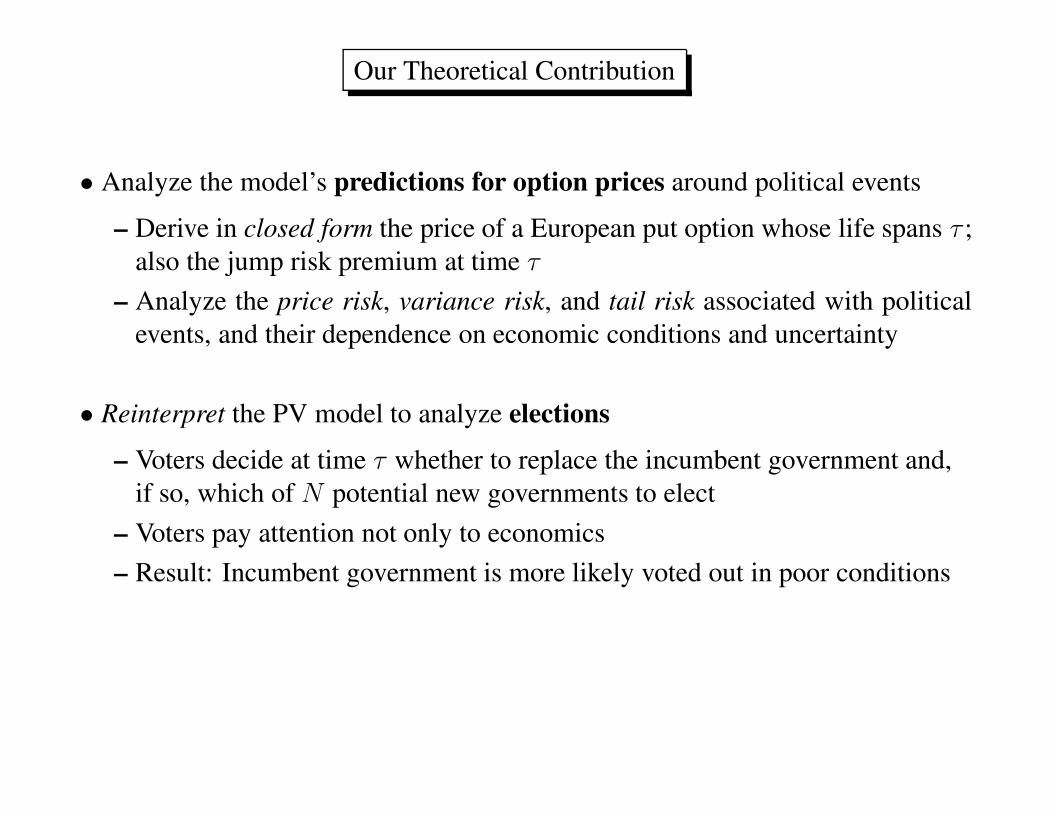
Our Theoretical Contribution

• Analyze the model’s predictions for option prices around political events

– Derive in closed form the price of a European put option whose life spans τ ;

also the jump risk premium at time τ

– Analyze the price risk, variance risk, and tail risk associated with political

events, and their dependence on economic conditions and uncertainty

• Reinterpret the PV model to analyze elections

– Voters decide at time τ whether to replace the incumbent government and,

if so, which of N potential new governments to elect

– Voters pay attention not only to economics

– Result: Incumbent government is more likely voted out in poor conditions

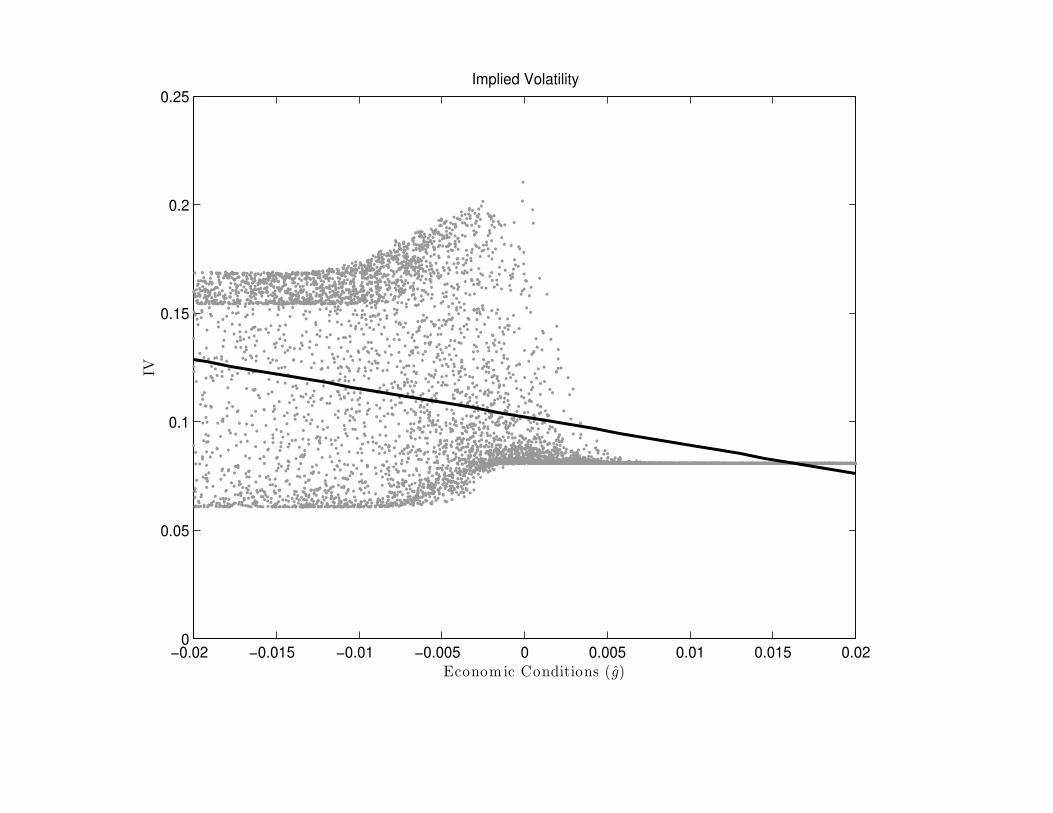
A Two-Policy Example

• Potential new policies H and L, same utility but H’s impact is more uncertain

• Same parameter values as in PV (2013)

• Simulate many paths of state variables in the model (gt,CH

t ,CL

t )

• For each simulated path, calculate three variables at time τ − 12 based on

one-period European put options that expire at time τ + 12

– IV : implied volatility of an ATM option (price risk)

– V RP : variance risk premium of an ATM option (variance risk)

∗ V RP = implied variance minus expected future variance

– Slope: implied volatility slope across strike prices (tail risk)

∗ Slope = implied vol 5% OTM minus implied vol 5% ITM

−0.02 −0.015 −0.01 −0.005 0 0.005 0.01 0.015 0.020

0.05

0.1

0.15

0.2

0.25Implied Volatility

IV

Economic Conditions (g)

−0.02 −0.01 0 0.01 0.02−0.02

−0.01

0

0.01

0.02

0.03

0.04Slope

Slope

Economic Conditions (g)−0.02 −0.01 0 0.01 0.02

−1.5

−1

−0.5

0

0.5

1Skewness of Returns

Skewness


−0.02 −0.01 0 0.01 0.02−0.01

0

0.01

0.02

0.03Variance Risk Premium

IV

2−E[V

ar]

Economic Conditions (g)−0.02 −0.01 0 0.01 0.02−1

0

1

2

3Jump Risk Premium

JRP


• Measure political uncertainty by the entropy of policy probabilities

Entropy = −pHt log pH

t − pLt log pL

t − p0t log p0

t , as of time t = τ − 12

0 0.2 0.4 0.6 0.8 10.06

0.08

0.1

0.12

0.14

0.16

0.18

0.2

0.22Implied Volatility

IV

Uncertainty

0 0.2 0.4 0.6 0.8 1−0.01

0

0.01

0.02

0.03

0.04Slope

Slope

Uncertainty

0 0.2 0.4 0.6 0.8 1−0.01

−0.005

0

0.005

0.01

0.015

0.02Variance Risk Premium

IV

2−E[V

ar]

Uncertainty

Data

• Options: 20 countries (from OptionMetrics)

– Put options on each country’s premier stock market index (for 15 countries)

or, if unavailable, ETF on the country’s MSCI index (for 5 countries)

• Political events

– National elections: parliamentary, presidential

– Global summits: G8, G20, European

• Economic conditions

– GDP : Realized real GDP growth (from OECD)

– FST : Forecast of real GDP growth (from IMF)

– CLI: Composite leading indicator (from OECD)

– MKT : Stock market index return (from Datastream)

• Political uncertainty: for elections only

– UNC: minus the poll spread (most recent opinion poll spread before the

election; if unavailable, then ex-post election margin)

Table 1: Option sample

Start End

Country Index Date Date

Australia ASX 200 20040102 20120604

Belgium BEL20 20020102 20120831

Brazil MSCI Brazil 20060525 20120131

Canada MSCI Canada 20060302 20120131

Finland OMXH25 20020102 20120831

France CAC 40 20030414 20120831

Germany DAX 20020102 20120831

Italy FTSE MIB 20061011 20120831

Japan NIKKEI 225 20040506 20120604

Korea Kospi 20040503 20120131

Mexico MSCI Mexico 20071129 20120131

Netherlands AEX 20020102 20120831

Singapore MSCI Singapore 20091118 20120131

South Africa MSCI South Africa 20070524 20120131

Spain IBEX 35 20070514 20120831

Sweden OMXS30 20070126 20120831

Switzerland SMI 20020102 20120831

Taiwan TAIEX 20040102 20120131

UK FTSE 100 20020102 20120831

USA S&P 500 19900101 20120131

Table 2: Number of political events

Elections Summits

Total Total Parl. Pres. Total Euro G8/G20

All 271 64 57 14 216 170 74

Australia 6 1 1 0 5 0 5

Belgium 13 2 2 0 11 11 0

Brazil 9 4 2 4 6 0 6

Canada 7 2 2 0 6 0 6

Finland 1 0 0 0 1 1 0

France 27 6 4 2 21 21 7

Germany 25 5 5 0 21 21 7

Italy 24 3 3 0 21 21 7

Japan 10 4 4 0 6 0 6

Korea 8 2 1 1 6 0 6

Mexico 7 1 1 0 6 0 6

Netherlands 22 3 3 0 19 19 0

Singapore 2 2 1 1 0 0 0

South Africa 6 1 1 0 5 0 5

Spain 20 4 4 0 17 17 0

Sweden 19 2 2 0 18 18 0

Switzerland 24 5 5 0 20 20 0

Taiwan 2 2 1 1 0 0 0

UK 24 4 4 0 21 21 7

USA 15 11 11 5 6 0 6

Option-Market Variables

a− s a

τ

b− s b c− s c

treatmentcontrol control

τ : political event date

a, b, c: option expiration dates

• Implied volatility difference:

IV Dτ = IV b −1

2(IV a + IV c) ,

where

IV b = Mean {IVb−s,b : b − s ∈ [τ − 20, τ − 1], ATM, open interest}

and IV a, IV c are defined analogously

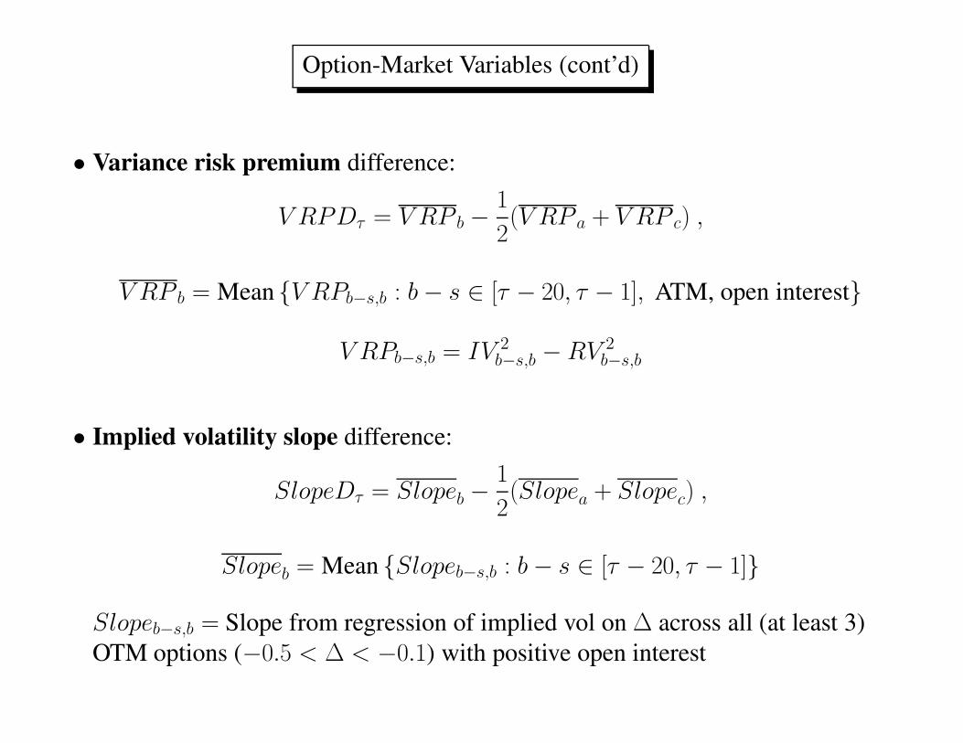
Option-Market Variables (cont’d)

• Variance risk premium difference:

V RPDτ = V RP b −1

2(V RP a + V RP c) ,

V RP b = Mean {V RPb−s,b : b − s ∈ [τ − 20, τ − 1], ATM, open interest}

V RPb−s,b = IV 2b−s,b − RV 2

b−s,b

• Implied volatility slope difference:

SlopeDτ = Slopeb −1

2(Slopea + Slopec) ,

Slopeb = Mean {Slopeb−s,b : b − s ∈ [τ − 20, τ − 1]}

Slopeb−s,b = Slope from regression of implied vol on ∆ across all (at least 3)

OTM options (−0.5 < ∆ < −0.1) with positive open interest

20 25 30 35 40 45 50Moneyness (|∆|)

Put Implied Volatility

IV no event

RV no event

VRP

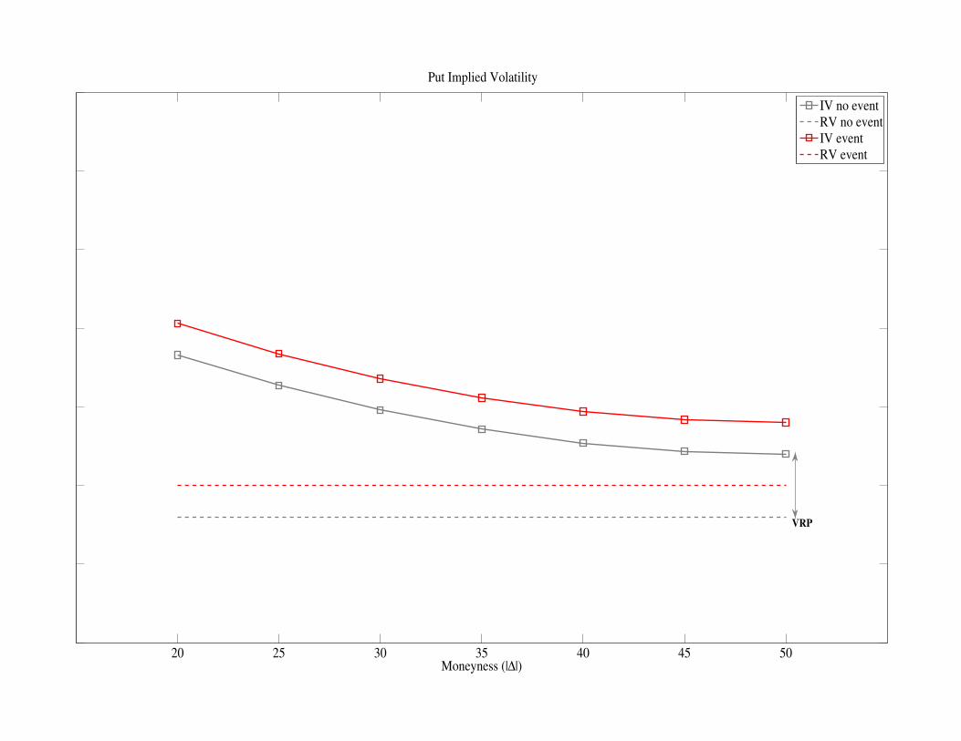
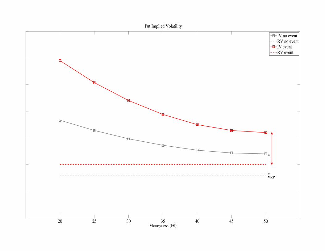
20 25 30 35 40 45 50Moneyness (|∆|)

Put Implied Volatility

IV no event

RV no event

IV event

RV event

VRP

Empirical Results

• We find empirical support for 8 of 9 theoretical predictions

• Political uncertainty is priced

– IV D is positive, on average

– V RPD is positive, on average

– SlopeD is positive, on average

• The price of political uncertainty is higher in weaker economic conditions

– IV D is larger when the economy is weaker

– V RPD is larger when the economy is weaker

– SlopeD is larger when the economy is weaker

• The price of political uncertainty is higher amid higher uncertainty

– IV D is larger when the election outcome is more uncertain

– V RPD is larger when the election outcome is more uncertain

Table 3: Mean implied volatility differences

Weak minus strong economy

All MKT GDP FST CLI

Panel A: All political events

Mean 1.43 2.57 1.94 2.22 3.00

(4.43) (3.79) (3.34) (3.78) (4.61)

Obs. 271 271 271 266 267

Panel B: Elections only

Mean 1.63 2.63 1.73 2.51 2.36

(3.13) (2.73) (1.78) (2.34) (2.39)

Obs. 64 64 64 59 60

Panel C: Summits only

Mean 1.42 2.68 2.13 2.40 3.25

(3.76) (3.27) (3.17) (3.56) (4.30)

Obs. 216 216 216 216 216



All MKT GDP FST CLI


Mean 1.43 2.57 1.94 2.22 3.00

(4.43) (3.79) (3.34) (3.78) (4.61)

Obs. 271 271 271 266 267

• Economic significance:

– ATM treatment-group options are more expensive by 5.1% compared to

control-group options, on average



All MKT GDP FST CLI


Mean 1.43 2.57 1.94 2.22 3.00

(4.43) (3.79) (3.34) (3.78) (4.61)

Obs. 271 271 271 266 267


Mean 1.63 2.63 1.73 2.51 2.36

(3.13) (2.73) (1.78) (2.34) (2.39)

Obs. 64 64 64 59 60


Mean 1.42 2.68 2.13 2.40 3.25

(3.76) (3.27) (3.17) (3.56) (4.30)

Obs. 216 216 216 216 216



All MKT GDP FST CLI


Mean 1.43 2.57 1.94 2.22 3.00

(4.43) (3.79) (3.34) (3.78) (4.61)

Obs. 271 271 271 266 267

• Economic significance:

– ATM treatment-group options are 7.1% to 9.0% more expensive compared

to control-group options when the economy is weak

– ATM treatment-group options are 0.1% to 1.2% more expensive compared

to control-group options when the economy is strong

Examples of Influential Political Events

• The crisis “combo”:

U.S. election (November 4, 2008; Obama vs. McCain)

G20 summit (November 14-15, 2008)

– Average IV D = 12.2%

• The pivotal Greek election (June 17, 2012)

– Average IV D = 6.7% (across European countries)

– Highest values: Spain (IV D = 10.3%) and Italy (7.7%)

– Lowest values: Sweden (IV D = 3.8%) and Switzerland (4.3%)

Table 4: Variance risk premium and implied volatility slope: Mean differencess

Variance risk premium (V RPD) Implied volatility slope (SlopeD)

Weak minus strong economy Weak minus strong economy

All MKT GDP FST CLI All MKT GDP FST CLI


Mean 1.07 3.02 2.07 2.55 3.05 1.73 3.26 2.11 2.66 3.02

(2.61) (3.51) (2.80) (3.54) (3.63) (3.59) (3.11) (2.52) (3.08) (2.97)

Obs. 271 271 271 266 267 238 238 238 233 236


Mean 1.30 2.46 1.07 2.45 1.26 1.14 3.56 1.14 1.96 1.38

(2.59) (2.62) (1.11) (2.20) (1.25) (2.08) (3.69) (1.08) (1.71) (1.28)

Obs. 64 64 64 59 60 55 55 55 50 53


Mean 1.07 3.39 2.58 2.97 3.75 1.84 3.43 2.53 2.87 3.46

(2.15) (3.15) (2.92) (3.49) (3.74) (3.16) (2.58) (2.54) (2.83) (2.80)

Obs. 216 216 216 216 216 191 191 191 191 191






Mean 1.07 3.02 2.07 2.55 3.05 1.73 3.26 2.11 2.66 3.02

(2.61) (3.51) (2.80) (3.54) (3.63) (3.59) (3.11) (2.52) (3.08) (2.97)

Obs. 271 271 271 266 267 238 238 238 233 236

• Economic significance (variance risk):

– ATM treatment-group options are 48.1% more expensive relative to the Black-

Scholes model, on average; control-group options are 36.5% more expensive






Mean 1.07 3.02 2.07 2.55 3.05 1.73 3.26 2.11 2.66 3.02

(2.61) (3.51) (2.80) (3.54) (3.63) (3.59) (3.11) (2.52) (3.08) (2.97)

Obs. 271 271 271 266 267 238 238 238 233 236

• Economic significance (tail risk):

– 5% (10%) OTM treatment-group options are more expensive by 9.6% (16.0%)






Mean 1.07 3.02 2.07 2.55 3.05 1.73 3.26 2.11 2.66 3.02

(2.61) (3.51) (2.80) (3.54) (3.63) (3.59) (3.11) (2.52) (3.08) (2.97)

Obs. 271 271 271 266 267 238 238 238 233 236


Mean 1.30 2.46 1.07 2.45 1.26 1.14 3.56 1.14 1.96 1.38

(2.59) (2.62) (1.11) (2.20) (1.25) (2.08) (3.69) (1.08) (1.71) (1.28)

Obs. 64 64 64 59 60 55 55 55 50 53


Mean 1.07 3.39 2.58 2.97 3.75 1.84 3.43 2.53 2.87 3.46

(2.15) (3.15) (2.92) (3.49) (3.74) (3.16) (2.58) (2.54) (2.83) (2.80)

Obs. 216 216 216 216 216 191 191 191 191 191

Panel A: Stock Market Return Panel B: GDP Growth

−0.5 −0.4 −0.3 −0.2 −0.1 0 0.1 0.2 0.3

−0.05

0.00

0.05

0.10

0.15

0.20

0.25

0.30

Economic Conditions

IVD

−5 −4 −3 −2 −1 0 1 2

−0.05

0.00

0.05

0.10

0.15

0.20

0.25

0.30

Economic Conditions

IVD

Panel C: GDP Growth Forecast Panel D: Composite Leading Indicator

−3 −2 −1 0 1 2

−0.05

0.00

0.05

0.10

0.15

0.20

0.25

0.30

Economic Conditions

IVD

−4 −3 −2 −1 0 1 2

−0.05

0.00

0.05

0.10

0.15

0.20

0.25

0.30

Economic Conditions

IVD

Table 5: Implied volatility difference and economic conditions

Measure of economic conditions

MKT GDP FST CLI


ECON -2.42 -3.58 -2.01 -2.71 -0.83 -0.63 -1.39 -1.47

(-5.34) (-5.10) (-4.82) (-5.01) (-2.55) (-1.37) (-3.85) (-2.74)

ECON · 1(ECON>0) 3.77 4.02 -0.96 0.26

(3.33) (3.85) (-0.87) (0.28)

R2 0.21 0.25 0.14 0.18 0.02 0.03 0.07 0.07

Obs. 271 271 271 271 266 266 267 267


ECON -1.72 -2.60 -1.56 -2.39 -1.69 -2.01 -1.34 -1.10

(-3.49) (-3.51) (-3.03) (-4.63) (-3.00) (-2.09) (-2.15) (-0.86)

ECON · 1(ECON>0) 2.69 3.26 1.18 -0.57

(1.62) (2.75) (0.61) (-0.34)

R2 0.17 0.20 0.14 0.18 0.15 0.16 0.12 0.13

Obs. 64 64 64 64 59 59 60 60


ECON -2.68 -3.93 -2.27 -3.02 -0.77 -0.54 -1.53 -1.88

(-5.04) (-4.86) (-4.84) (-5.08) (-2.10) (-1.10) (-3.91) (-3.18)

ECON · 1(ECON>0) 4.16 4.61 -1.26 1.23

(3.24) (3.89) (-0.95) (1.04)

R2 0.23 0.28 0.17 0.20 0.02 0.02 0.08 0.08

Obs. 216 216 216 216 216 216 216 216


−0.5 −0.4 −0.3 −0.2 −0.1 0 0.1 0.2 0.3

−0.20

−0.10

0.00

0.10

0.20

0.30

Economic Conditions

VR

PD

−5 −4 −3 −2 −1 0 1 2

−0.20

−0.10

0.00

0.10

0.20

0.30

Economic Conditions

VR

PD


−3 −2 −1 0 1 2

−0.20

−0.10

0.00

0.10

0.20

0.30

Economic Conditions

VR

PD

−4 −3 −2 −1 0 1 2

−0.20

−0.10

0.00

0.10

0.20

0.30

Economic Conditions

VR

PD

Table 6: Variance risk premium difference and economic conditions


MKT GDP FST CLI


ECON -2.98 -4.55 -1.97 -2.43 -1.32 -1.40 -1.72 -2.23

(-4.56) (-4.45) (-3.52) (-3.40) (-3.42) (-2.50) (-3.38) (-2.88)

ECON · 1(ECON>0) 5.10 2.62 0.35 1.75

(3.41) (1.67) (0.27) (1.44)

R2 0.19 0.24 0.08 0.09 0.04 0.04 0.06 0.07

Obs. 271 271 271 271 266 266 267 267


ECON -1.62 -2.22 -1.32 -2.79 -1.78 -1.76 -1.18 -1.79

(-2.34) (-1.90) (-1.78) (-3.80) (-2.69) (-1.70) (-1.51) (-1.18)

ECON · 1(ECON>0) 1.86 5.79 -0.09 1.40

(0.92) (3.73) (-0.05) (0.70)

R2 0.16 0.18 0.11 0.25 0.18 0.18 0.09 0.10

Obs. 64 64 64 64 59 59 60 60


ECON -3.45 -5.27 -2.32 -2.67 -1.40 -1.53 -2.01 -2.69

(-4.52) (-4.53) (-3.67) (-3.39) (-3.13) (-2.48) (-3.56) (-3.08)

ECON · 1(ECON>0) 6.07 2.17 0.71 2.37

(3.59) (1.18) (0.46) (1.56)

R2 0.22 0.28 0.10 0.10 0.04 0.04 0.07 0.08

Obs. 216 216 216 216 216 216 216 216


−0.5 −0.4 −0.3 −0.2 −0.1 0 0.1 0.2 0.3−0.10

−0.05

0.00

0.05

0.10

0.15

0.20

0.25

0.30

0.35

0.40

Economic Conditions

Slo

peD

−5 −4 −3 −2 −1 0 1 2−0.10

−0.05

0.00

0.05

0.10

0.15

0.20

0.25

0.30

0.35

0.40

Economic Conditions

Slo

peD


−3 −2 −1 0 1 2−0.10

−0.05

0.00

0.05

0.10

0.15

0.20

0.25

0.30

0.35

0.40

Economic Conditions

Slo

peD

−4 −3 −2 −1 0 1 2−0.10

−0.05

0.00

0.05

0.10

0.15

0.20

0.25

0.30

0.35

0.40

Economic Conditions

Slo

peD

Table 7: Implied volatility slope difference and economic conditions


MKT GDP FST CLI


ECON -3.19 -5.37 -2.20 -2.77 -0.78 -0.32 -1.62 -1.96

(-3.82) (-4.21) (-3.02) (-2.87) (-1.66) (-0.48) (-2.47) (-1.89)

ECON · 1(ECON>0) 6.86 3.11 -2.15 1.08

(3.62) (1.83) (-1.34) (0.66)

R2 0.19 0.26 0.09 0.10 0.01 0.02 0.05 0.05

Obs. 238 238 238 238 233 233 236 236


ECON -2.11 -1.70 -1.21 -2.34 -0.31 -0.18 -0.98 -1.05

(-5.26) (-2.13) (-2.22) (-3.50) (-0.42) (-0.16) (-1.70) (-0.81)

ECON · 1(ECON>0) -1.17 3.38 -0.48 0.12

(-0.77) (2.13) (-0.19) (0.07)

R2 0.27 0.28 0.09 0.15 0.01 0.01 0.06 0.06

Obs. 55 55 55 55 50 50 53 53


ECON -3.54 -6.15 -2.49 -3.01 -0.88 -0.28 -1.78 -2.20

(-3.58) (-4.28) (-3.01) (-2.86) (-1.66) (-0.38) (-2.41) (-1.88)

ECON · 1(ECON>0) 8.42 3.13 -3.10 1.41

(3.95) (1.63) (-1.68) (0.69)

R2 0.19 0.28 0.10 0.10 0.01 0.02 0.05 0.05

Obs. 191 191 191 191 191 191 191 191

−0.4 −0.3 −0.2 −0.1 0

−0.08

−0.06

−0.04

−0.02

0.00

0.02

0.04

0.06

0.08

0.10

0.12

UNC

IVD

−0.4 −0.3 −0.2 −0.1 0

−0.04

−0.02

0.00

0.02

0.04

0.06

0.08

0.10

0.12

0.14

0.16

UNC

VR

PD

−0.25 −0.2 −0.15 −0.1 −0.05 0

−0.10

−0.08

−0.06

−0.04

−0.02

0.00

0.02

0.04

0.06

0.08

0.10

UNC

Slo

peD

Table 8: The role of election uncertainty


MKT GDP FST CLI

Panel A: Implied volatility (IV D)

UNC 1.87 1.64 1.58 1.80 1.82 1.68 1.69 1.44 1.45

(5.39) (4.52) (4.43) (4.93) (4.49) (4.11) (4.28) (3.21) (3.14)

ECON -1.46 -2.17 -1.47 -2.34 -1.36 -1.72 -1.52 -1.61

(-2.98) (-2.85) (-3.27) (-5.57) (-2.45) (-1.89) (-3.26) (-1.77)

ECON · 1(ECON>0) 2.14 3.41 1.34 0.22

(1.39) (2.65) (0.80) (0.17)

R2 0.20 0.31 0.34 0.32 0.37 0.29 0.30 0.26 0.26

Obs. 64 64 64 64 64 59 59 60 60



MKT GDP FST CLI

Panel B: Variance risk premium (V RPD)

UNC 1.06 0.82 0.78 0.99 1.03 0.74 0.74 0.89 1.00

(3.48) (2.39) (2.32) (2.54) (2.31) (1.91) (1.89) (1.75) (1.76)

ECON -1.49 -2.01 -1.27 -2.76 -1.64 -1.63 -1.29 -2.15

(-2.10) (-1.66) (-1.75) (-3.90) (-2.38) (-1.58) (-1.80) (-1.66)

ECON · 1(ECON>0) 1.59 5.87 -0.02 1.95

(0.79) (3.69) (-0.01) (1.09)

R2 0.07 0.20 0.21 0.17 0.32 0.21 0.21 0.14 0.17

Obs. 64 64 64 64 64 59 59 60 60



MKT GDP FST CLI

Panel C: Implied volatility slope (SlopeD)

UNC 0.25 -0.11 -0.14 0.07 0.11 0.25 0.24 0.23 0.24

(0.59) (-0.33) (-0.39) (0.17) (0.27) (0.50) (0.47) (0.56) (0.57)

ECON -2.13 -1.71 -1.20 -2.33 -0.28 -0.17 -0.98 -1.07

(-5.08) (-2.12) (-2.16) (-3.39) (-0.36) (-0.15) (-1.67) (-0.82)

ECON · 1(ECON>0) -1.20 3.40 -0.39 0.18

(-0.78) (2.13) (-0.16) (0.10)

R2 0.00 0.27 0.28 0.09 0.15 0.01 0.01 0.06 0.06

Obs. 55 55 55 55 55 50 50 53 53

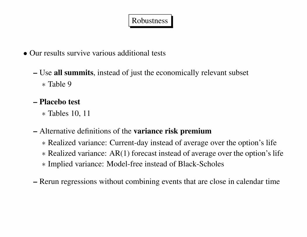
Robustness

• Our results survive various additional tests

– Use all summits, instead of just the economically relevant subset

∗ Table 9

– Placebo test

∗ Tables 10, 11

– Alternative definitions of the variance risk premium

∗ Realized variance: Current-day instead of average over the option’s life

∗ Realized variance: AR(1) forecast instead of average over the option’s life

∗ Implied variance: Model-free instead of Black-Scholes

– Rerun regressions without combining events that are close in calendar time

Table 9: Robustness: All summitsMeasure of economic conditions

MKT GDP FST CLI

Panel A: IV D

ECON -1.85 -3.28 -1.74 -2.51 -0.69 -0.44 -1.13 -1.72

(-4.11) (-4.44) (-4.46) (-4.97) (-2.54) (-1.18) (-3.49) (-3.36)

ECON · 1(ECON>0) 4.00 4.27 -1.16 1.82

(3.69) (4.42) (-1.13) (1.97)

R2 0.14 0.19 0.12 0.16 0.02 0.02 0.05 0.06

Obs. 310 310 310 310 310 310 310 310

Panel B: V RPD

ECON -2.76 -4.72 -2.03 -2.36 -1.10 -1.06 -1.82 -2.74

(-4.53) (-4.62) (-3.98) (-3.55) (-3.42) (-2.25) (-4.05) (-3.55)

ECON · 1(ECON>0) 5.50 1.79 -0.16 2.82

(3.88) (1.29) (-0.13) (2.27)

R2 0.18 0.25 0.10 0.10 0.03 0.03 0.08 0.09

Obs. 310 310 310 310 310 310 310 310

Panel C: SlopeD

ECON -2.44 -4.95 -1.98 -2.55 -0.82 -0.22 -1.37 -2.17

(-2.91) (-3.64) (-2.94) (-2.86) (-2.11) (-0.38) (-2.36) (-2.18)

ECON · 1(ECON>0) 6.93 3.03 -2.80 2.34

(3.60) (1.92) (-1.88) (1.43)

R2 0.11 0.19 0.07 0.08 0.01 0.02 0.03 0.04

Obs. 273 273 273 273 273 273 273 273

Table 10: Placebo events and mean differences


All MKT GDP FST CLI

Panel A: IV D

Mean (data) 1.43 2.57 1.94 2.22 3.00

Mean (pseudo-events) -0.32 1.35 -0.63 -1.63 -1.03

Difference 1.75 1.22 2.57 3.85 4.03

p-value <0.001 0.017 <0.001 <0.001 <0.001

Obs. 271 271 271 266 267

Panel B: V RPD

Mean (data) 1.07 3.02 2.07 2.55 3.05

Mean (pseudo-events) -0.26 0.21 -0.11 -0.44 -0.61

Difference 1.33 2.81 2.18 2.99 3.66

p-value <0.001 <0.001 <0.001 <0.001 <0.001

Obs. 271 271 271 266 267

Panel C: SlopeD

Mean (data) 1.73 3.26 2.11 2.66 3.02

Mean (pseudo-events) -0.31 0.41 -0.65 0.59 -0.46

Difference 2.04 2.85 2.75 2.06 3.48

p-value <0.001 0.005 <0.001 <0.001 <0.001

Obs. 238 238 238 233 236

Table 11: Placebo events and economic conditions


MKT GDP FST CLI

Panel A: IV D

ECON Data -2.42 -3.58 -2.01 -2.71 -0.83 -0.63 -1.39 -1.47

Placebo -0.89 -1.29 0.77 1.21 0.81 0.95 0.79 1.10

Difference -1.53 -2.29 -2.77 -3.92 -1.64 -1.58 -2.18 -2.57

p-value <0.001 <0.001 <0.001 <0.001 <0.001 <0.001 <0.001 <0.001

ECON · Data 3.77 4.02 -0.96 0.26

1(ECON>0) Placebo 1.00 -1.55 -0.32 -0.73

Difference 2.77 5.57 -0.64 0.99

p-value <0.001 <0.001 0.593 0.102

Obs. 271 271 271 271 266 266 267 267

Panel B: V RPD

ECON Data -2.98 -4.55 -1.97 -2.43 -1.32 -1.40 -1.72 -2.23

Placebo -0.30 -0.51 0.51 0.88 0.38 0.73 0.47 1.12

Difference -2.68 -4.03 -2.48 -3.31 -1.70 -2.12 -2.19 -3.35

p-value <0.001 <0.001 <0.001 <0.001 0.002 0.003 0.001 0.002

ECON · Data 5.10 2.62 0.35 1.75

1(ECON>0) Placebo 0.68 -1.55 -0.72 -1.64

Difference 4.42 4.17 1.07 3.39

p-value 0.002 0.026 0.067 0.004

Obs. 271 271 271 271 266 266 267 267

Panel C: SlopeD

ECON Data -3.19 -5.37 -2.20 -2.77 -0.78 -0.32 -1.62 -1.96

Placebo -0.67 -1.00 0.71 1.27 0.52 0.71 0.74 1.22

Difference -2.52 -4.37 -2.91 -4.03 -1.30 -1.03 -2.36 -3.17

p-value <0.001 <0.001 <0.001 <0.001 <0.001 0.014 <0.001 <0.001

ECON · Data 6.86 3.11 -2.15 1.08

1(ECON>0) Placebo 0.55 -1.29 -0.83 -1.51

Difference 6.31 4.40 -1.31 2.59

p-value <0.001 <0.001 0.601 0.001

Obs. 238 238 238 238 233 233 236 236

Conclusions

• Political uncertainty is priced in the option market in ways predicted by theory

• Options whose lives span political events offer valuable protection against

– price risk

– variance risk

– tail risk

associated with major political events

• This protection is more valuable

– when the economy is weaker

– when political uncertainty is higher

The Price of Political Uncertainty: Theory and Evidence...

Documents

Transcript of The Price of Political Uncertainty: Theory and Evidence...