The Price of Pessimism for Multidimensional Quadrature

625

⁄ 0885-064X/01 $35.00© 2001 Elsevier ScienceAll rights reserved.

journal of complexity 17, 625–659 (2001)

doi:10.1006/jcom.2001.0593, available online at http://www.idealibrary.com on

The Price of Pessimism for Multidimensional Quadrature

Fred J. Hickernell1

1 This research was supported in part by Hong Kong Research Grants Council GrantRGC/HKBU/2030/99P and Hong Kong Baptist University Grant FRG/97-98/II-99.

Department of Mathematics, Hong Kong Baptist University, Kowloon Tong,Hong Kong SAR, ChinaE-mail: [email protected]

URL: http://www.math.hkbu.edu.hk/~fred

and

Henryk Wozniakowski2

2 This author was supported in part by the National Science Foundation.

Department of Computer Science, Columbia University, New York, New York 10027; andInstitute of Applied Mathematics, University of Warsaw, ul. Banacha 2,

02-097, Warsaw, PolandE-mail: [email protected]

URL: http://www.cs.columbia.edu/~henryk

Published online September 14, 2001

Multidimensional quadrature error for Hilbert spaces of integrands is studied inthree settings: worst-case, random-case, and average-case. Explicit formulae arederived for the expected errors in each case. These formulae show the relative, pes-simism of the three approaches. The first is the trace of a hermitian and nonnega-tive definite matrix LmQ, the second is the spectral radius of the same matrix L

mQ, and

the third is the trace of the matrix SLmQ for a hermitian and nonnegative matrix S

with trace (S)=1. Several examples are studied, including Monte Carlo quadratureand shifted lattice rules. Some of the results for Hilbert spaces of integrands can beextended to Banach spaces of integrands. © 2001 Elsevier Science

1. INTRODUCTION

Multidimensional integration has attracted much attention due to itsapplicability to problems in finance [2, 4, 20 25, 26, 28, 35], in physics andengineering [16, 17, 27, 34] and in statistics [6, 7]. Suppose that onewishes to compute the integral

I(f) — FXf(x) dF(x), (1.1)

in the Stieltjes sense, where f is some measurable function, the integrationdomain, X, is some measurable subset of R s, and F(x) is some probabilitydistribution with >X dF(x)=1. If this integral is too complicated toevaluate by analytic means, then one might compute some approximation,Q(f), that depends on n evaluations of the integrand. This approximationmight be based on a Gaussian rule, a Monte Carlo rule, a quasi-MonteCarlo rule, a Smolyak rule, etc., all of which take the form

Q(f) — Cn

i=1aif(xi), (1.2)

where x1, ..., xn are the nodes where the integrand is evaluated, anda1, ..., an are some predetermined weights.One might like to know how good the approximation is, i.e., how small

is the error, Err(f; Q) — I(f)−Q(f). Although one may answer this ques-tion for a particular integrand and quadrature rule, such an answer haslimited applicability. Thus, we will consider sets of integrand and sets ofquadrature rules.The integrands, f, will be assumed to lie in some normed linear spaceH

of measurable functions. We usually assume that H is a separable Hilbertspace. Two cases will be considered. One case considers the worst integrandlying in the unit ball:

F={f ¥H : ||f||H [ 1}. (1.3)

The other case considers the integrand to be randomly chosen from Haccording to a probability measure such that the mean square norm ofintegrands is one.The nodes and/or the weights in the quadrature rule are often chosen

randomly. Examples of random rules include simple Monte Carlo quadra-ture, randomly shifted lattice rules [5], scrambled (t, s)-sequences [23],random start Halton sequences [38], etc. Random quadrature rules can

626 HICKERNELL AND WOZNIAKOWSKI

facilitate quadrature error estimation as well as error analysis. In thisarticle the quadrature rules are assumed to be chosen randomly from asample space Q with a probability measure m. Of course, deterministic rulescan be recovered by assuming that Q contains a single rule.Given the assumptions on the integrand and the quadrature rule, there

are three interesting error measures one may consider:

eworst — rmsQ ¥ Q

supf ¥F

|Err(f; Q)|, (1.4a)

e rand — supf ¥F

rmsQ ¥ Q

|Err(f; Q)|, (1.4b)

eavg — rmsQ ¥ Q

rmsf ¥H

|Err(; Q)|, (1.4c)

For worst-case error, (1.4a), one fixes Q, and computes the error for theworst integrand. Then one takes the root mean square, denoted by rms in(1.4), over quadrature rules with respect to the measure m. For random-caseerror, one considers the root mean square error over Q for each integrand,and then computes the worst error over all integrands from the unit ball.Average-case error takes the root mean square error over both integrandsand quadrature rules.To guarantee that the errors in (1.4) are well defined, we assume that the

corresponding quantities are measurable. The measurability assumptionwill easily follow for the spaces of functions considered in this paper.Let e denote any of the three error measures defined in (1.4). The quality

of a set of quadrature formulae, Q, is determined by how e depends in par-ticular on n, the number of function evaluations used in the quadratureformula, and s, the number of variables. One might wish to computee=e(n, s) explicitly for a particular H and Q or find the asymptotic orderof e(n, s) for large n and/or s.It is obvious that

eworst \ e rand \ eavg.

Thus, the number of quadrature points, n, required to obtain a satisfactoryerror will be greatest according to eworst, less according to e rand, and leastaccording to eavg. Thus, the worst-case error is the most pessimistic cri-terion, random-case error is less pessimistic, and the average-case error isthe most optimistic. The disadvantage of an optimistic criterion is that thepredicted n may not give the required error for a specific integrand andquadrature rule. On the other hand, the price of a pessimistic criterion isthat the computation may cost too many function evaluations. Fromanother point of view, integration may be difficult according to a more

PRICE OF PESSIMISM 627

pessimistic criterion, whereas it may be easy according to a more optimisticone. The purpose of this article is to understand the relative pessimism ofthe three criteria presented in (1.4).Sections 2, 3, and 4 cover worst-case error, random-case error, and

average-case error, respectively, where H is a Hilbert space. The casewhereH is a Banach space is discussed briefly in Section 5.This paper reviews and unifies some results that have appeared elsewhere

as indicated in the text. It also presents new results that are previewedbelow. The new results hold when H is a Hilbert space unless otherwisenoted:

i. It is shown that the error measure eworst is the square root of thetrace of a matrix, LmQ, that depends only on Q and the basis ofH (Theorem2.2). Moreover, e rand is the square root of the spectral radius of the samematrix LmQ (Theorem 3.2), and eavg is the square root of the trace of SLmQwith trace (S)=1 (Theorem 4.1). This gives a quantitative explanation ofthe relative pessimism of eworst, e rand, and eavg.

ii. It is known that for reproducing kernel Hilbert spacessupf ¥F |Err(f; Q)| is equal to the discrepancy D(Q; K), a quantitydepending only on the quadrature rule, Q, and the reproducing kernel, K,of the space H (see e.g., [13, 37]). Certain rules, Q, are obtained byrandomizing a deterministic quasi-Monte Carlo quadrature rule, Qinit.Theorem 2.3 shows that eworst=rmsQ ¥ Q D(Q; K)=D(Qinit; Kran). In otherwords eworst is simply the discrepancy of Qinit based on a filtered version ofthe reproducing kernel. This principle has been observed before in specialcases [9, 15], and it greatly facilitates the computation of eworst.

iii. In general, computing the spectral radius of LmQ to find e rand isdifficult. However, for certain choices of bases dependent on the quadra-ture rule, the matrix LmQ becomes diagonal, which facilitates the computa-tion of its spectral radius. It is shown in Section 3.1 that choosing a basisthat makes LmQ diagonal is equivalent to performing an analysis of variance(ANOVA) decomposition of the quadrature error.

iv. For Monte Carlo quadrature it is known that all three errormeasures in (1.4) are proportional to n−1/2. For eavg the constant of pro-portionality can be interpreted as the root mean square average standarddeviation of an integrand in H, and for e rand the constant of proportio-nality is the largest possible standard deviation of integrands in F. Thesetwo facts are previously known. It is shown here that for eworst the constantof proportionality is the largest possible standard deviation for anintegrand that is the sum of mutually orthogonal functions lying inF.

v. In the Hilbert space setting one typically has eworst > e rand, exceptfor trivial cases such as ifH is one dimensional or Q is a deterministic rule.


However, it is shown in the remarks following Corollary 5.2 that in certainBanach spaces eworst=e rand, i.e., worst-case error is no more pessimisticthan random-case error.

We end this introduction by stressing that in this paper we study theexpected error of quadrature formulas and we do not address the choice ofa quadrature formula with the minimal error. The reader interested in theminimal error quadrature formulas is referred to a recent survey by Novakand Wozniakowski [22] for the worst case, to the books [21, 36] for therandomized case, and to a recent book by Ritter [29] for the average casesetting.

2. WORST-CASE ERROR

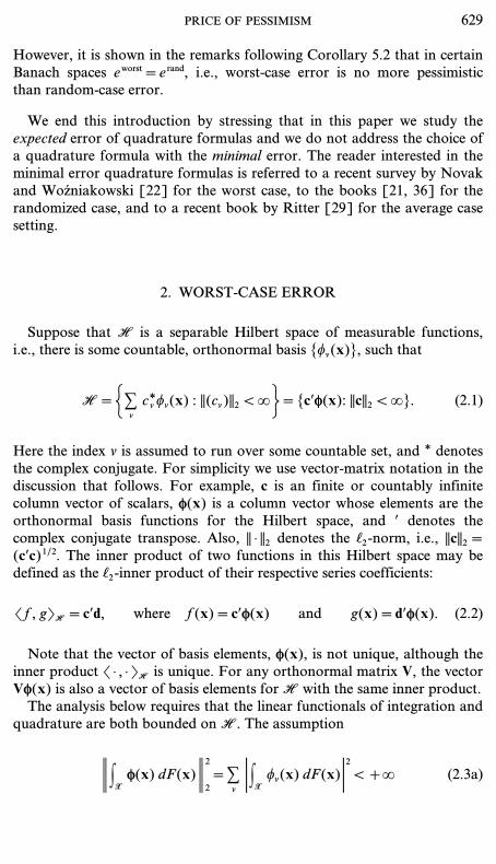
Suppose that H is a separable Hilbert space of measurable functions,i.e., there is some countable, orthonormal basis {fn(x)}, such that

H=3Cn

cgn fn(x) : ||(cn)||2 <.4={cŒf(x): ||c||2 <.}. (2.1)

Here the index n is assumed to run over some countable set, and * denotesthe complex conjugate. For simplicity we use vector-matrix notation in thediscussion that follows. For example, c is an finite or countably infinitecolumn vector of scalars, f(x) is a column vector whose elements are theorthonormal basis functions for the Hilbert space, and Œ denotes thecomplex conjugate transpose. Also, || · ||2 denotes the a2-norm, i.e., ||c||2=(cŒc)1/2. The inner product of two functions in this Hilbert space may bedefined as the a2-inner product of their respective series coefficients:

Of, gPH=cŒd, where f(x)=cŒf(x) and g(x)=dŒf(x). (2.2)

Note that the vector of basis elements, f(x), is not unique, although theinner product O · , ·PH is unique. For any orthonormal matrix V, the vectorVf(x) is also a vector of basis elements forH with the same inner product.The analysis below requires that the linear functionals of integration and

quadrature are both bounded onH. The assumption

>FXf(x) dF(x)>

2

2=C

n

:FXfn(x) dF(x) :

2

<+. (2.3a)


implies that I as defined in (1.1) is a bounded, linear functional. Theassumption

||f(x)||22=Cn

|fn(x)|2 <+. -x ¥X, (2.3b)

implies that the functional evaluating f at an arbitrary point is bounded.This in turn implies that any quadrature rule of the form (1.2) is abounded, linear functional. In the rest of the article we assume that themeasurable functions fn satisfy (2.3a) and (2.3b).

2.1. Discrepancy

For any integrand f(x)=cŒf(x) ¥H, the quadrature error using aquadrature rule Q is

Err(f; Q)=cŒ Err(f; Q), (2.4)

since both integration and quadrature are bounded linear functionals onH. Here and below, the Err functional and other functionals applied to avector or matrix are assumed to apply term-by-term. Under the assump-tions (2.3a) and (2.3b) the function

tQ(x)=[Err(f; Q)]Œ f(x) (2.5)

lies in the Hilbert spaceH, and in fact, is the representer of the quadratureerror for rule Q, i.e.,

Err(f; Q)=Of, tQPH -f ¥H. (2.6)

Starting either from (2.4) or (2.6) one may apply the Cauchy–Schwarzinequality to obtain a sharp upper bound on the quadrature error of theform

|Err(f; Q)| [ D(Q) ||f||H -f ¥H, (2.7)

where the discrepancy, is defined as

D(Q) — ||tQ ||H=||Err(f; Q)||2 (2.8a)

={[Err(f; Q)]Œ Err(f; Q)}1/2=5Cn

|Err(f; Q)|261/2

(2.8b)

={trace(Err(f; Q)[Err(f; Q)]Œ)}1/2. (2.8c)

The discrepancy is also the norm of the linear functional Err( · ; Q).


Recall that the set of integrands F is the unit ball in the Hilbert space,(1.3). It follows that

supf ¥F

|Err(f; Q)|=D(Q), (2.9)

which appears in (1.4a). The worst-case error measure eworst is the rootmean square discrepancy and is discussed in Section 2.2.The reason for the name discrepancy is now explained. For any quadra-

ture rule Q of the form (1.2) define

FQ(y)=Q(1(−/, y])=Cn

i=1ai1[xi, −/)(y) -y ¥X,

where 1A is the indicator function of a set A. Here and elsewhere (−/, y]denotes the set of vectors x, such that xj [ yj for all j. If Q is a quasi-Monte Carlo rule of the form

Qqmc: Q(f) —1nCn

i=1f(xi), (2.10)

then FQ is simply the empirical distribution of the node set {x1, ..., xn}. Thequadrature rule may be expressed as integration in terms of FQ, i.e.,Q(f)=>Xf(x) dFQ(x). Thus, the quadrature error may be expressed as

Err(f; Q)=I(f)−Q(f)=FXf(x) d(F−FQ)(x). (2.11)

Referring to the definition of the discrepancy in (2.8), one can now see thatit measures how much FQ differs from F. Thus, the discrepancy is small ifFQ is close to F. In fact, one may interpret the discrepancy as a norm ofF−FQ [10].Since the vector of basis elements satisfies condition (2.3b), the Hilbert

spaceH has a reproducing kernel defined as:

K(x, y)=fŒ(x) f(y). (2.12)

The reproducing kernel of a Hilbert space has the following properties [3,29, 30, 37]:

K( · , y) ¥H -y ¥X,

Reproducing Property: f(y)=Of, K( · , y)PH -f ¥H, y ¥X,


and also,

Symmetry: K(x, y)=K*(y, x) -x, y ¥X, (2.13a)

Positive Definiteness: Cn

i, j=1aia

gj K(xi, xj) \ 0 -ai ¥ R, xi ¥X.

(2.13b)

The reproducing kernel of a Hilbert space is unique, even though the basis{fn((x)} is not. Moreover, any function satisfying conditions (2.13) is thereproducing kernel of some Hilbert space.By (2.5), (2.11) and (2.12) it follows that tQ(x)=>X K(x, y) d(F−FQ)(y),

and so the discrepancy may be written in terms of the reproducing kernelas:

D(Q)=[Erry(Errx(K(x, y); Q); Q)]1/2 (2.14a)

=5FXK(x, y) d(F−FQ)(x) d(F−FQ)(y)6

1/2

. (2.14b)

The discrepancy may be also written in terms of integrals and sums overthe reproducing kernel:

D(Q)=5FX

2K(x, y) dF(x) dF(y)−2 C

n

i=1ai F

XK(xi, y) dF(y)

+ Cn

i, j=1aiajK(xi, xj)6

1/2

. (2.15)

From (2.8) it is clear that the discrepancy is the root sum of squarequadrature errors of the orthonormal basis, {fn}. In fact, the discrepancy isthe maximum root sum of square quadrature errors for any set of ortho-normal functions, {kn}, which is not necessarily a basis, i.e.,

D(Q)=sup 3 ||Err(k; Q)||2==Cn

|Err(kn; Q)|2

: k=(kn), kn ¥H, Okg, knPH=dgn 4. (2.16)

To see why this is true, note that ||Err(k; Q)||2 is the norm of the projectionof tQ into the subspace ofH spanned by {kn}. Thus, ||Err(k; Q)||2 [ ||tQ ||H=D(Q), with equality holding iff tQ is in the span of {kn}.Many formulas of this section are basically known. The main points are

summarized in the following theorem:


Theorem 2.1. Suppose that H is a separable Hilbert space with basis{fn} and inner product O · , ·PH, as defined in (2.1) and (2.2), and that thebasis satisfies conditions (2.3). Then H has a unique reproducing kernel, K,defined in (2.12). Furthermore, for quadrature rules of the form (1.2) theerror is a bounded, linear functional on H with representer tQ, defined in(2.5). The quadrature error is bounded by inequality (2.7), which may also bewritten as (2.9). The quality of the quadrature rule is given by its dis-crepancy, D(Q), which can be expressed equivalently in terms of the basis orthe reproducing kernel, see (2.8), (2.14), (2.15) and (2.16).

2.2. Average Discrepancy

By error bound (2.9) the quantity eworst defined in (1.4a) is simply theroot mean square discrepancy, D(Q)=D(Q; K), i.e.,

eworst=rmsQ ¥ Q

D(Q)==FQD2(Q) dm(Q),

if we assume that D(Q) is measurable with respect to the s-field of m. Wenow comment on this measurability assumption. From (2.15) and (2.12) iteasily follows that it is enough to assume that the function ;n

i=1 aifn(xi) ismeasurable for any n. This implies that ;n

i=1 aif(xi) is measurable for anyf from H. In what follows we will consider the classes Q of quadratureformulas with fixed ai=n−1 and with random sample points xi which are,for example, independent and uniformly distributed over X=[0, 1] s. Sinceall practically important functions fn are continuous the measurabilityassumption holds.Assuming measurability of D(Q), at an abstract level one may use (2.8)

to express this as follows:

Theorem 2.2. The error measure eworst may be expressed as the squareroot of the trace of a matrix

eworst=`trace(LmQ) , (2.17)

where the hermitian and nonnegative definite matrix LmQ is defined as

LnQ=FQErr(f; Q)[Err(f; Q)]Œ dm(Q). (2.18)


Moreover, one can write eworst in terms of the worst possible sum of the rootmean square errors of an orthogonal set of functions in H:

eworst=sup 3=Cn

[rmsQ ¥ Q

|Err(kn; Q)|]2

: {kn} …H, Okg, knPH=dgn 4 . (2.19)

Proof. Equation (2.17) follows from (2.8), and then (2.19) followsfrom (2.16). L

The matrix LmQ also appears in the formula (3.1) for e rand and formula(4.4) for eavg below. However, the above formula for eworst is not necessarilyeasy to compute since LnQ is usually infinite dimensional. Equation (2.15)expressing the discrepancy in terms of the reproducing kernel is moreuseful for calculating eworst. However, direct calculation is often not the bestapproach.We now show how eworst can be computed for certain random quadrature

rules. Suppose that for any set of n points, Pinit ıX, one has a randomiza-tion algorithm that results in the random set of n points, P={xz: z ¥ Pinit}.Here, xz is a random point from X. The randomized set P can then be usedto form a randomized quasi-Monte Carlo rule:

Q(f; P) —1n

Cz ¥ Pinit

f(xz). (2.20)

There are several randomized rules of this form including most of the onesmentioned in the introduction. The discrepancy is a quadratic form of xz.To compute its average we need to know the distribution of (xz, xt) as wellas of xz.For every (z, t) ¥X×X, with z ] t, it is assumed that there exists Fzt, the

joint distribution function for the random points (xz, xt) ¥X×X, and Fz,the marginal distribution for the point xz ¥X. For z=t it follows that

Fzz(x, y)=Fz(min(x, y))=Fz(min(x1, y1), ..., min(xs, ys)). (2.21)

Here and elsewhere min(x, y) means componentwise minimization.Some mild assumptions are made about these two distributions. First, it

assumed that Fzt has a symmetry in its arguments, i.e., the order of thepoints does not matter:

Fzt(x, y)=Ftz(y, x) -z, t, x, y ¥X. (2.22a)


It is also assumed that the random ordered pair, (xz, xt) averaged over thepre- randomized point, z, has its two components independently distrib-uted, the first is Fz-distributed and the second is F-distributed,

FXFzt(x, y) dF(t)=Fz(x) F(y) -z, x, y ¥X. (2.22b)

Finally it is assumed that xz averaged over the pre-randomized point z isF-distributed, i.e.,

FXFz(x) dF(z)=F(x) -x ¥X. (2.22c)

As we shall see, in some cases not only is (2.22c) satisfied, but in factFz=F, which makes the random rule unbiased.Under these assumptions one has Theorem 2.3 below for calculating the

root mean square discrepancy of a random rule.Theorem 2.3. Consider quadrature rules of the form (2.20), where the

random set P is obtained from an initial set Pinit by the randomization algo-rithm satisfying conditions (2.22). Let Qinit denote the quasi-Monte Carloquadrature rule corresponding to Pinit. Then the root mean square discrepancyof these quadrature rules is just the discrepancy of the initial set,

eworst=rmsQ ¥ Q

D(Q; K)=D(Qinit; Kran), (2.23)

where the new reproducing kernel, Kran, is obtained by filtering the originalkernel:

Kran(z, t)=FX

2K(x, y) d2Ftz(x, y)=E[K(xt, xz)] -z, t ¥X.

If, in addition, Kran(z, t)=K(z, t) for all z, t ¥X, then this reproducingkernel is called randomization-invariant and

eworst=rmsQ ¥ Q

D(Q; K)=D(Qinit; K). (2.24)

Proof. By (2.15) the square discrepancy of the initial quadrature ruleQinit under the filtered kernel may be written as the sum of three terms:

D2(Qinit; Kran)=FX

2Kran(x, y) dF(x) dF(y)

−2n

Cz ¥ Pinit

FXKran(z, y) dF(y)+

1n2 C

z, t ¥ Pinit

Kran(z, t).


By interchanging the order of integration and applying conditions (2.22),the first term can be re-written as

FX

2Kran(t, z) dF(t) dF(z)=F

X2FX

2K(x, y) d2Ftz(x, y) dF(t) dF(z)

=FX

2K(x, y) dF(x) dF(y).

the second term may be re-written as

−2n

Cz ¥ Pinit

FXKran(z, t) dF(t)

=−2n

Cz ¥ Pinit

FXFX

2K(x, y) d2Ftz(y, x) dF(t)

=−2n

Cz ¥ Pinit

FXE[K(xz, y)] dF(y),

and the third term may be re-written (for z=t we use (2.21)) as:

1n2 C

z, t ¥ Pinit

Kran(z, t)=1n2 C

z, t ¥ Pinit

E[K(xz, xt)].

These three terms summed together form E[D2(Q)], the mean square dis-crepancy of the random rule Q. This completes the proof of (2.23). Theproof of (2.24) is straightforward. L

2.3. Examples

2.3.1. Monte Carlo quadrature. Consider the example of simple MonteCarlo quadrature, i.e.,

Qmc: Q(f) —1nCn

i=1f(xi), (2.25)

where the xi are independent and identically distributed random variableswith distribution function F. Let Lmc denote the corresponding matrix LmQas defined in (2.18). It is straightforward to show that

Lmc=1nCov(f), (2.26)


where the covariance of a vector of functions is defined as:

Cov(f)=I(ffŒ)−I(f) I(fŒ)

=1FX[fg(x)−I(fg)][f

gn (x)−I(fg

n )] dF(x)2 .

From Theorem 2.2 it then follows that

eworstmc — eworst= rmsQ ¥ Q

mcD(Q)

=1

n1/2`trace(Cov(f))=1

n1/2=C

n

Var(fn), (2.27)

where Var denotes the variance of a function:

Var(f)=I(f2)−[I(f)]2=FXf2(x) dF(x)−5F

Xf(x) dF(x)6

2

.

From another perspective one may also apply Theorem 2.3 to MonteCarlo quadrature. In this case Pinit is any set of n discrete points, xz, xt areindependent random variables on X with the distributions

Fzt(x, y)=F(x) F(y) for z ] t,

Fzz(x, y)=F(min(x, y)), Fz(x)=F(x).

The filtered kernel is

Kmc(z, t)=˛FX2K(x, y) dF(x) dF(y), z ] t.

FXK(x, x) dF(x), z=t.

The Hilbert space corresponding to this filtered kernel is in general notseparable even though the original Hilbert space, H, is. Nonetheless, onemay apply Theorem 2.3 to compute the root mean square discrepancy forMonte Carlo quadrature:

Corollary 2.4. Consider simple Monte Carlo quadrature rules, Q, ofthe form (2.25), or equivalently (2.20), where the random set P is a set of nindependent and identically distributed points on X. Then


eworstmc — eworst=

1n1/2`trace(Cov(f))

= rmsQ ¥ Q

mcD(Q; K)=D(Qinit; Kmc)

=1

n1/23F

XK(x, x) dF(x)−F

X2K(x, y) dF(x) dF(y)4

1/2

,

where Qinit denotes the quasi-Monte Carlo quadrature rule corresponding toany set of n distinct points, Pinit. One may identify the quantity in bracesabove as

FXK(x, x) dF(x)−F

X2K(x, y) dF(x) dF(y)

=sup 3Cn

Var(kn) : {kn} …H, Okg, knPH=dgn 4 . (2.28)

Proof. The proof of (2.28) follows from (2.19) and (2.26). L2.3.2. The weighted Korobov space. Consider uniform integration, i.e.,

X=[0, 1] s and F(x)=x1 · · · xs, over the space of periodic functions, HKor,generated by the trigonometric polynomial basis elements

fn(x)=e2pinŒx[(b−1/a1 n1) · · · (b

−1/as ns)]−a/2, a > 1, (2.29)

where

x — ˛|x|, x ] 0,

1, x=0.

Larger values of the parameter a imply greater smoothness of theintegrands. The parameters b1, ..., bs are assumed to be positive, andreflect the significance of the different coordinates. The reproducing kernelHKor, is

KKor(x, y)= Cn ¥ Zs

e2pinŒ(x−y) [(b−1/a1 n1) · · · (b

−1/as ns)]−a. (2.30)

For this basis the covariance matrix appearing in (2.26) is diagonal:

Lmc−Kor=(Cov(fg, fn))

n

=1n(dgn(1−d0n)[(b

−1/a1 n1) · · · (b

−1/as ns)]−a). (2.31)


The trace of this matrix may be computed in terms of the Riemann-zetafunction, z. Corollary 2.4 then gives

eworstmc−Kor(n, s)=1

`n3 −1+D

s

j=1[1+2bjz(a)]4

1/2

.

A plot of eworstmc−Kor(n, s) versus n for several choices of s is given in Fig. 1 inSection 4.2 below.

2.3.3. Gain coefficients. Owen [24] introduced the concept of gaincoefficients to compare randomized quasi-Monte Carlo rules to simpleMonte Carlo. For an arbitrary set of random quadrature rules, Q, definethe gain coefficients, CmQn, in terms of the mean square error of the basiselements:

CmQ=(CmQn), where CmQn=[rmsQ ¥ Q |Err(fn; Q)|]2

Var(fn)/n. (2.32)

Here we adopt the convention that 0/0=0. The gain coefficients are justthe diagonal elements LmQ divided by the respective diagonal elements ofLmc. If we assume that Var(fn)=0 implies that rmsQ ¥ Q Err(fn; Q)=0,then the root mean square discrepancy can be written as

eworst=rmsQ ¥ Q

D(Q)=1

n1/2 [Cm−Q Var(f)]

1/2

=1

n1/25Cn

CmQn Var(fn)61/2

,

where Var(f)=(Var(fn)). By definition, the gain coefficients for simpleMonte Carlo are unity, i.e. CmcQn=1. This, the gain coefficient CmQn measureshow well a randomized quadrature rule integrates the basis element fn incomparison to simple Monte Carlo. If the gain coefficient CnQn is greaterthan one, then the quadrature rules Q amplify the error with respect tosimple Monte Carlo, and if the gain coefficient CmQn is less than one, thenthe quadrature rules Q damp the error with respect to simple Monte Carlo.

2.3.4. Null quadrature. A trivial quadrature rule takes Qnull(f)=0 forall integrands f. Although this might seem to be a useless rule, it might bepreferable when the integrands are very complex, and one does not havethe budget to take enough function evaluations to get any other reason-able estimate. Assuming the space of quadrature rules, Q, consists of onlythe null rule, then the matrix LmQ appearing in (2.18) is

Lnull=I(f) I(fŒ).


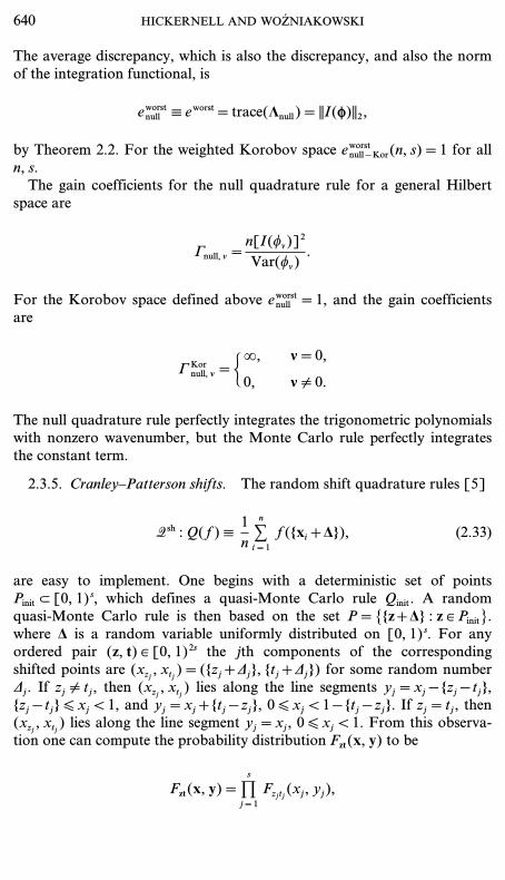
The average discrepancy, which is also the discrepancy, and also the normof the integration functional, is

eworstnull — eworst=trace(Lnull)=||I(f)||2,

by Theorem 2.2. For the weighted Korobov space eworstnull−Kor(n, s)=1 for alln, s.The gain coefficients for the null quadrature rule for a general Hilbert

space are

Cnull, n=n[I(fn)]2

Var(fn).

For the Korobov space defined above eworstnull =1, and the gain coefficientsare

CKornull, n=˛., n=0,

0, n ] 0.

The null quadrature rule perfectly integrates the trigonometric polynomialswith nonzero wavenumber, but the Monte Carlo rule perfectly integratesthe constant term.

2.3.5. Cranley–Patterson shifts. The random shift quadrature rules [5]

Q sh : Q(f) —1nCn

i=1f({xi+D}), (2.33)

are easy to implement. One begins with a deterministic set of pointsPinit … [0, 1) s, which defines a quasi-Monte Carlo rule Qinit. A randomquasi-Monte Carlo rule is then based on the set P={{z+D} : z ¥ Pinit}.where D is a random variable uniformly distributed on [0, 1) s. For anyordered pair (z, t) ¥ [0, 1)2s the jth components of the correspondingshifted points are (xzj , xtj )=({zj+Dj}, {tj+Dj}) for some random numberDj. If zj ] tj, then (xzj , xtj ) lies along the line segments yj=xj − {zj −tj},{zj −tj} [ xj < 1, and yj=xj+{tj −zj}, 0 [ xj < 1− {tj −zj}. If zj=tj, then(xzj , xtj ) lies along the line segment yj=xj, 0 [ xj < 1. From this observa-tion one can compute the probability distribution Fzt(x, y) to be

Fzt(x, y)=Ds

j=1Fzjtj (xj, yj),


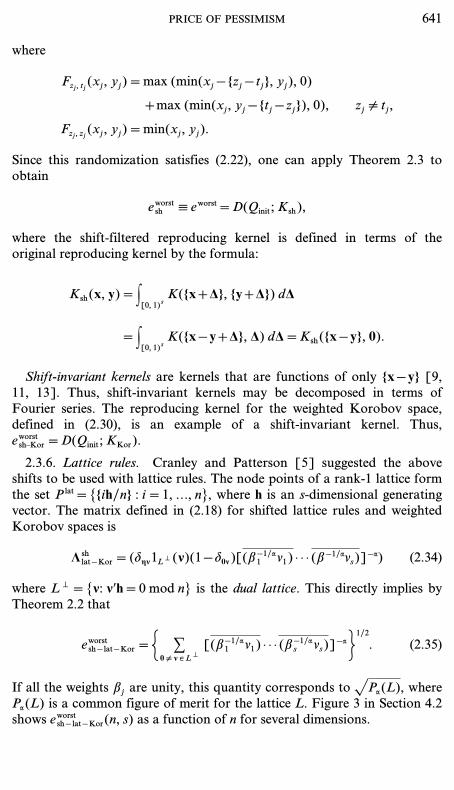
where

Fzj, tj (xj, yj)=max (min(xj − {zj −tj}, yj), 0)

+max (min(xj, yj − {tj −zj}), 0), zj ] tj,

Fzj, zj (xj, yj)=min(xj, yj).

Since this randomization satisfies (2.22), one can apply Theorem 2.3 toobtain

eworstsh — eworst=D(Qinit; Ksh),

where the shift-filtered reproducing kernel is defined in terms of theoriginal reproducing kernel by the formula:

Ksh(x, y)=F[0, 1)s

K({x+D}, {y+D}) dD

=F[0, 1)s

K({x−y+D}, D) dD=Ksh({x−y}, 0).

Shift-invariant kernels are kernels that are functions of only {x−y} [9,11, 13]. Thus, shift-invariant kernels may be decomposed in terms ofFourier series. The reproducing kernel for the weighted Korobov space,defined in (2.30), is an example of a shift-invariant kernel. Thus,eworstsh–Kor=D(Qinit; KKor).

2.3.6. Lattice rules. Cranley and Patterson [5] suggested the aboveshifts to be used with lattice rules. The node points of a rank-1 lattice formthe set P lat={{ih/n} : i=1, ..., n}, where h is an s-dimensional generatingvector. The matrix defined in (2.18) for shifted lattice rules and weightedKorobov spaces is

L shlat−Kor=(dgn1L + (n)(1−d0n)[(b−1/a1 n1) · · · (b−1/ans)]−a) (2.34)

where L +={n: nŒh=0mod n} is the dual lattice. This directly implies byTheorem 2.2 that

eworstsh− lat−Kor=3 C0 ] n ¥ L +

[(b−1/a1 n1) · · · (b

−1/as ns)]−a41/2. (2.35)

If all the weights bj are unity, this quantity corresponds to `Pa(L), wherePa(L) is a common figure of merit for the lattice L. Figure 3 in Section 4.2shows eworstsh− lat−Kor(n, s) as a function of n for several dimensions.


The gain coefficients for randomly shifted lattice rules for the weightedKorobov space are the diagonal elements L shlat−Kor divided by the respectivediagonal element of Lmc−Kor, i.e.,

C sh−Korlat =(n1L + (n)(1−d0n)). (2.36)

Thus lattice rules damp to zero the quadrature error for basis elements withwavenumber, n, not in the dual lattice, but amplify the quadrature error forbasis elements with wavenumber n in the dual lattice.

2.3.7. The weighted Sobolev space. Several scholars have studied quad-rature rules for integrands in Sobolev spaces. The weighted Sobolev space,HSob, as defined by Sloan and Wozniakowski [32], has the reproducingkernel

KSob(x, y)=Ds

j=1{1+bj[1−max (xj, yj)]},

where again the bj are positive weights. The discrepancy defined by thiskernel is the weighted L2-star discrepancy.The corresponding shift-filtered reproducing kernel for the weighted

Sobolev space, as derived by Hickernell [9], is

KSob, sh(x, y)=Ds

j=1{1+bj[

13+B2({xj −yj})]},

where B2 is the second degree Bernoulli polynomial [1, Chap. 23],B2(x)=x2−x+1/6. This kernel is equivalent to the reproducing kernel forthe weighted Korobov space defined in (2.30). Specifically, if one chooses

a=2, b0=Ds

j=1

11+bj

32 , bj=

bj

2p2(1+bj/3), j=1, 1..., s,

then KSob, sh(x, y)=b0KKor(x, y). Since the two reproducing kernels areequivalent, then the quadrature error measures are equivalent, namelyeworstSob (n, s)=b1/2

0 eworstKor (n, s). This equivalence is exploited in the investiga-tions of [13, 14, 33].

3. RANDOM-CASE ERROR

This section looks at the error measure e rand defined in (1.4b). Again it isassumed that the integrands lie in the unit ball,F, of a Hilbert spaceH of


measurable functions for which (2.3) hold. However, this time the quadra-ture error is first averaged over the quadrature rules, and then oneconsiders the worst case integrand.

3.1. Mean Square Errors and ANOVA Decompositions

For any particular integrand, f ¥H, the root mean square quadratureerror can be written as the sum of two terms:

rmsQ ¥ Q

|Err(f; Q)|=ÈQ ¥ Q{[I(f)−Q(f)]2}

=`[I(f)−Q(f)]2+EQ ¥ Q{[Q(f)−Q(f)]2}

=`Bias(f; Q)+Var(f; Q) ,

where Q(f)=EQ ¥ Q[Q(f)] is the mean quadrature in the class Q.The first term in the above equation is the systematic bias of the quad-

rature rule, while the second is the variance of the quadrature rule. Deter-ministic rules have, in general, nonzero bias, but zero variance, while well-chosen random rules, such as Monte Carlo, Cranley–Patterson shifts,Owen’s scrambling, etc., have zero bias and nonzero variance.From another perspective one may start with the series representation of

the quadrature error given by (2.4) and obtain

rmsQ ¥ Q

|Err(f; Q)|=ÈQ ¥ Q{cŒErr(f; Q)[Err(f; Q)]Œ c}=`cŒLmQc, (3.1)

where the matrix LmQ is defined in (2.18). So, one may express erand as

e rand=supf ¥F

ÈQ ¥ Q[|Err(f; Q)|2]= sup||c||2=1

`cŒLmQc=`r(LmQ) ,

where r( · ) denotes the spectral radius.In general it may be difficult to compute the spectral radius of the matrix

LmQ. However, the problem simplifies in the case where this matrix isdiagonal. In such a situation one may think of the series representation ofan arbitrary integrand f ¥H as an analysis of variance (ANOVA)decomposition of the quadrature error.

Definition 3.1. A basis {fn} is called ANOVA-consistent for ran-domized quadrature rules if and only if LmQ is a diagonal matrix, i.e.,

EQ ¥ Q[Err(fg; Q) Err(fn; Q)]=dgnEQ ¥ Q[|Err(fn; Q)|2].

For ANOVA-consistent bases, the decomposition of the integrandf(x)=cŒf(x) is a sum of ANOVA effects, fn(x)=cg

n fn(x). The root mean


square quadrature error for the random quadrature rule Q is the squareroot of the sum of the mean square quadrature errors of the ANOVAeffects, i.e.,

rmsQ ¥ Q

|Err(f; Q)|==Cn

[rmsQ ¥ Q

|Err(fn; Q)|]2

==Cn

|cv |2 [rmsQ ¥ Q

|Err(fn; Q)|]2 .

If the random quadrature rule Q is unbiased, then rmsQ ¥ Q |Err(f; Q)| issimply the standard deviation of the quadrature error. The followingtheorem summarizes the above results.

Theorem 3.2. If F is the unit ball in a Hilbert space satisfying (2.3)then the error measure e rand may be expressed in terms of the spectral radiusof the matrix LmQ:

e rand=`r(LmQ) . (3.2)

Furthermore, if {fn} is an ANOVA-consistent basis for the randomizedquadrature rules Q, then

e rand=supn

rmsQ ¥ Q

|Err(fn; Q)|= supf ¥H

||f||H [ 1

rmsQ ¥ Q

|Err(f; Q)|.

3.2. Examples Revisited

Recall from (2.26) that for simple Monte Carlo quadrature the matrixLmQ is L

mc=Cov(f)/n, so

e randmc =`r(Cov(f))

`n. (3.3)

A set of basis elements {fn} is ANOVA- consistent for the simple MonteCarlo quadrature rules if and only if Cov(f) is a diagonal matrix. If abasis, {fn}, is ANOVA-consistent for simple Monte Carlo, then thedecomposition of an arbitrary function, f=;n fn, fn=cg

n fn, is anANOVA decomposition of f in the traditional sense, i.e., the variance of fis the sum of the variance of its ANOVA effects, fn:

Var(f)=cŒ Cov(f) c=Cn

|cn |2 Var(fn)=Cn

Var(fn).


Given a reproducing kernel for the Hilbert space H, one may constructa set of basis elements that are ANOVA-consistent with simple MonteCarlo quadrature rules by solving the following eigenvalue problem:

FX[K(x, y)−I(K(x, · ))][fn(y)−I(fn)] dF(y)=lnfn(x),

FX[fg(x)−I(fg)][f

gn (x)−I(fgn )] dF(x)=dgnln.

The basis (2.29) used to define the weighted Korobov space is ANOVA-consistent for simple Monte Carlo quadrature. By inspecting thecovariance matrix Cov(f) as given in (2.31) it follows that

e randmc−Kor(n, s)=min(1, maxj bj)

`nDs

j=1max (bj, 1).

which is the largest bj times the product of all other bj which are greaterthan 1 times n−1/2, see also [33]. Figure 1 displays plots of e randmc−Kor(n, s)versus n.Since null quadrature is a deterministic rule, the approach to quadrature

error taken in this section and the previous one are the same, i.e.,eworstnull (n, s)=e randnull (n, s) for any Hilbert space. For the weighted Korobovspace, eworstnull−Kor=e randnull−Kor=1, independent of s, and of course, of n.If a set of basis elements happens to be ANOVA-consistent for

some arbitrary randomized quadrature rule and also for simple MonteCarlo rules, then the gain coefficients defined in (2.32) may be used toexpress e rand:

e rand=1

n1/2`supn

[CQn Var(fn)] .

The basis (2.29) used to define the weighted Korobov space is ANOVA-consistent for randomly-shifted lattice rules, as well as for simple MonteCarlo quadrature. From the formula for the L shlat−Kor in (2.34), or equiva-lently, from the formula for the gain coefficients (2.36), it follows that:

e randsh− lat−Kor=[ min0 ] n ¥ L +

(b−1/a1 n1) · · · (b

−1/as ns)]−a.

For the case b1=·· ·=bs=1 this is [rZar(L)]−a, where rZar is theZaremba figure of merit for lattices [18, 31]. Figure 3 showse randsh− lat−Kor(n, s) as a function of n for several values of s and all bj=1.


4. AVERAGE-CASE ERROR

In this section the integrand is assumed to be a random function. Thesample space of random integrands H arising in (1.4c) is just the Hilbertspace H satisfying (2.3) from the previous sections, but now one allowsrandom coefficients cn in the series expansion f(x)=cŒf(x). Suppose thatthe random vector c has zero mean and a specified covariance matrix, S:

Ef ¥H(c)=0, and Cov(c)=S, where trace(S)=1. (4.1)

The condition on the trace of S insures that the root mean square norm ofrandom functions f equals one, since

rmsf ¥H

||f||H=`Ef ¥H[||f||2H]=`E[||c||22]=`trace(Cov(c))=1.

The sample space of random integrands H arising in (1.4c) is then just theHilbert space H, but the random integrands have root mean square normof one.

4.1. Covariance Kernel

It is known that for a fixed quadrature rule taking the average error overthe space of random integrands equals a discrepancy that is similar to theone defined in Section 2.1 [29]. Specifically,

Ef ¥H[|Err(f; Q)|2]=Ef ¥H{[Err(f; Q)]Œ ccŒErr(f; Q)}

=[Err(f; Q)]Œ S Err(f; Q)

=D2(Q; K), (4.2)

where

K(x, y)=fŒ(x) Sf(y) (4.3)

is the reproducing kernel defined as in (2.12), but now for the vector ofbasis elements S1/2f. Note that this kernel is well defined due to (2.3b) andmay be considered to be a covariance kernel, since

Ef ¥H[f(x)]=E(cŒ) f(x)=0 -x ¥X,

Ef ¥H[f(x) f(y)]=E[fŒ(x) ccŒf(y)]=fŒ(x) Sf(y)

=K(x, y) -x, y ¥X.


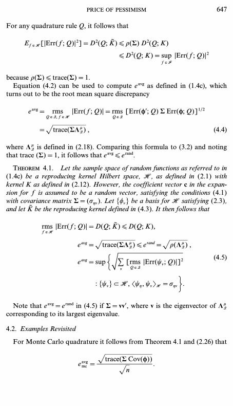
For any quadrature rule Q, it follows that

Ef ¥H[|Err(f; Q)|2]=D2(Q; K) [ r(S) D2(Q; K)

[ D2(Q; K)=supf ¥F

|Err(f; Q)|2

because r(S) [ trace(S)=1.Equation (4.2) can be used to compute eavg as defined in (1.4c), which

turns out to be the root mean square discrepancy

eavg= rmsQ ¥ Q, f ¥H

|Err(f; Q)|=rmsQ ¥ Q

[Err(fŒ; Q) S Err(f; Q)]1/2

=`trace(SLmQ) , (4.4)

where LmQ is defined in (2.18). Comparing this formula to (3.2) and notingthat trace (S)=1, it follows that eavg [ e rand.

Theorem 4.1. Let the sample space of random functions as referred to in(1.4c) be a reproducing kernel Hilbert space, H, as defined in (2.1) withkernel K as defined in (2.12). However, the coefficient vector c in the expan-sion for f is assumed to be a random vector, satisfying the conditions (4.1)with covariance matrix S=(sgn). Let {fn} be a basis for H satisfying (2.3),and let K be the reproducing kernel defined in (4.3). It then follows that

rmsf ¥H

|Err(f; Q)|=D(Q; K) [ D(Q; K),

eavg=`trace(SLmQ) [ e rand=`r(LmQ) ,

eavg=sup 3=Cn

[rmsQ ¥ Q

|Err(kn; Q)|]2

: {kn} …H, Okg, knPH=sgn 4 .

(4.5)

Note that eavg=e rand in (4.5) if S=vvŒ, where v is the eigenvector of LmQcorresponding to its largest eigenvalue.

4.2. Examples Revisited

For Monte Carlo quadrature it follows from Theorem 4.1 and (2.26) that

eavgmc=`trace(S Cov(f))

`n.


This is no larger than both eworstmc in (2.27) and e randmc in (3.3). Suppose that Sis a diagonal matrix with elements

sgn=˛{[1+2z(c)] s−1}−1 [n1 · · · ns]−c, g=n ] 0,0, otherwise,

(4.6)

where z is the Riemann zeta function and c > 1. Note that trace (S)=1.Then for the Korobov space eavgmc may be calculated explicitly as

eavgmc−Kor=1

`n`[1+2z(c)] s−1=−1+D

s

j=1[1+2bjz(a+c)].

Figure 1 displays plots of eworstmc−Kor(n, s), erandmc−Kor(n, s), and eavgmc−Kor(n, s)

versus n for several choices of s, and for a=c=2 and bj=1. As expectedthese are straight lines, indicating the n−1/2 error decay rates of MonteCarlo quadrature. However, the constants in front are different for dif-ferent dimensions and for different error measures. As the dimension in-creases, eworstmc−Kor(n, s) exponentially increases, indicating the fact that worst-case integration becomes more difficult. The quantity e randmc−Kor(n, s)=n−1/2 is

FIG. 1. Performance of Monte Carlo quadrature for the weighted Korobov space, HKor,with a=c=2 and b1=·· ·=bs=1: eworstmc−Kor(n, s) (solid), e

randmc−Kor(n, s) (dashed), e

avgmc−Kor(n, s)

(dot-dashed) for s=1, 2, 4, 8.


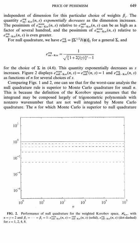
independent of dimension for this particular choice of weights bj. Thequantity eavgmc−Kor(n, s) exponentially decreases as the dimension increases.The pessimism of eworstmc−Kor(n, s) relative to e randmc−Kor(n, s) can be as high as afactor of several hundred, and the pessimism of eworstmc−Kor(n, s) relative toeavgmc−Kor(n, s) is even greater.For null quadrature, we have eavgnull=||S1/2I(f)||2 for a general S, and

eavgmc−Kor=1

`[1+2z(c)] s−1

for the choice of S in (4.6). This quantity exponentially decreases as sincreases. Figure 2 displays eworstnull−Kor(n, s)=e randnull (n, s)=1 and eavgnull−Kor(n, s)as functions of n for several choices of s.Comparing Figs. 1 and 2, one can see that for the worst-case analysis the

null quadrature rule is superior to Monte Carlo quadrature for small n.This is because the definition of the Korobov space assumes that theintegrand may be composed largely of trigonometric polynomials withnonzero wavenumber that are not well integrated by Monte Carloquadrature. The n for which Monte Carlo is superior to null quadrature

FIG. 2. Performance of null quadrature for the weighted Korobov space, HKor, witha=c=2 and b1=·· ·=bs=1: eworstnull−Kor(n, s)=

randnull−Kor(n, s) (solid), e

avgnull−Kor(n, s) (dot-dashed)

for s=1, 2, 4, 8.


exponentially increases with the dimension, s, for bj=1. However, if the bj

are made small enough, i.e.

Ds

j=1(1+2bjz(a)) < 2,

then Monte Carlo quadrature is superior to null quadrature in the worst-case analysis for all n.For the random-case analysis null quadrature is never better than Monte

Carlo if all bj [ 1. On the other hand, if some bj are larger than 1 then nullquadrature can still be substantially better than Monte Carlo for small n,even in the random-case analysis. A similar result holds for the average-case analysis.For randomly shifted lattice rules eavg has a similar form to that of eworst

in (2.35):

eavgsh− lat−Kor=3{[1+2z(c)] s−1}−1 C0 ] n ¥ L +

[(b−1/a1 n1) · · · (b

−1/as ns)]−a− c41/2.

If all the weights bj are unity, this quantity corresponds to

eavgsh− lat−Kor=`{[1+2z(c)] s−1}−1 Pa+c(L) .

where Pa(L) is a common figure of merit for the lattice L.Figure 3 shows eworstsh− lat−Kor(n, s), e

randsh− lat−Kor(n, s), and eavgsh− lat−Kor(n, s) as a

function of n for several dimensions. The generating vector for thisparticular lattice is

h=(1, 17797, 177972, ..., 17797 s−1),

which was suggested by Hickernell et al. [12]. In all three cases the errormeasures increase with increasing dimension. Note that eworstsh− lat−Kor(n, s) maybe substantially larger than e randsh− lat−Kor(n, s) and e randsh− lat−Kor(n, s) may besubstantially larger than eavgsh− lat−Kor(n, s). Note that in the one dimensionalcase eavgsh− lat−Kor(n, 1) % n−2, whereas eworstsh− lat−Kor(n, 1) % n−1.Comparing Figs. 1, 2 and 3 one sees that lattice rules, like Monte Carlo

quadrature, are also worse than the null quadrature rule for small n for theworst-case error analysis when bj — 1. However, under the random-caseerror analysis, shifted lattice rules always beat null quadrature for thischoice of the bj. For random-case error lattice rules are sometimes worsethan Monte Carlo quadrature because of the large gain coefficients for


FIG. 3. Performance of a randomly shifted lattice rule for the weighted Korobov space,HKor, with a=c=2 and b1=·· ·=bs=1: eworstsh− lat−Kor(n, s) (solid), e

randsh− lat−Kor(n, s) (dashed),

eavgsh− lat−Kor(n, s) (dot-dashed) for s=1, 2, 4, 8 and n=1, 2, ..., 217.

wavenumbers in the dual lattice. Unlike the cases of Monte Carlo and nullquadrature, eavgsh− lat−Kor(n, s) increases as the dimension increases for theaverage-case analysis.

5. EXTENSIONS OF THE RESULTS TO BANACH SPACES

The results in the previous sections can be extended to certain Banachspaces defined in a similar manner as (2.1). For any 1 [ q [., let p satisfyp−1+q−1=1, and define

Hq=3Cn

cgn fn(x) : ||(cn)||p <.4={cŒf(x): ||c||p <.}, (5.1)

where || · ||p denotes the ap-norm. Furthermore, define the norm on thisBanach space by ||cŒf(x)||Hq

=||c||p. This definition implies that for a fixedbasis

Hq `Hr for all 1 [ q [ r [..


The case p=q=2 corresponds to the Hilbert space defined in (2.1). For ageneral q, we also consider unit balls of functions Fq, as defined as in (1.3)Assumptions (2.3) now become

>FXf(x) dF(x)>

q

q=C

n

:FXf(x) dF(x) :

q

<+., (5.2a)

||f(x)||qq=Cn

|fn(x)|q <+. -x ¥X. (5.2b)

First, we consider the worst-case error analysis, analogous to Section 2.By applying Hölder’s inequality one may obtain a worst-case error boundanalogous to that in (2.7):

|Err(f; Q)| [ Dp(Q) ||f||Hq-f ¥Hq,

where the discrepancy is now defined as Dp(Q) — ||Err(f; Q)||q. The dis-crepancy is also the norm of the linear functional Err( · ; Q). From thedefinition of the aq-norm it follows that the Dp(Q) [ Dr(Q) for p [ r for afixed quadrature rule, Q.Computing the root mean square discrepancy for a random quadrature

rule Q for the case q ] 2 is difficult, except in the special case where

Dp(Q)=Dp(Qinit) with probability one (5.3)

for some deterministic rule Qinit. This happens when, for example,

|Err(f; Q)|=|Err(f; Qinit)| with probability one.

The above condition is satisfied for quadrature rules, Q, which are randomshifts of a quasi-Monte Carlo rule, Qinit, and where the basis, {fn}, is thatused to define the Korobov space. Under condition (5.3) it follows that

eworstq =Dp(Qinit).

Next, we perform a random-case error analysis like what was done inSection 3. If one computes the root mean square error of a random quad-rature rule for some integrand inHq, then one obtains as in (3.1):

rmsQ ¥ Q

|Err(f; Q)|=`EQ ¥ Q[cŒ Err(f; Q) Err(fŒ; Q) c]=`cŒLmQc .


Taking the supremum over integrands in the unit ball Fq, is in general dif-ficult. However, if the basis is ANOVA-consistent, i.e., LmQ is diagonal, thenHölder’s inequality may be used to obtain

e randq =supf ¥Fq

`EQ ¥ Q[|Err(f; Q)|2]= sup||c||p=1

`cŒLmQc

== sup||c||p=1

Cn

|cn |2 lmQnn=||(lmQnn)||r,

where the lmQnn are the diagonal elements of LmQ , and

r=˛q

2−q, 1 [ q < 2,

., 2 [ q [..

(5.4)

The results of the above two paragraphs are combined in the followingtheorem.

Theorem 5.1. Consider a Banach space of integrands, Hq, as defined in(5.1). If the discrepancy satisfies (5.3), then, eworst

q =Dp(Qinit), wherep=q/(q−1). If the basis, {fn}, is ANOVA-consistent, then e rand

q =||(lmQnn)||r,where r is defined in (5.4).

Corollary 5.2. If the discrepancy satisfies (5.3), and also the basis isANOVA-consistent, then e rand

q =eworstr , where r is defined in (5.4).

Under the conditions of Corollary 5.2 we have eworstq =Dp(Qinit) ande rand=Dy(Qinit), where

y=˛q

2(q−1), 1 [ q < 2,

1, 2 [ q [..

Moreover, for 1 [ q <. it follows that p > y, which is to be expected, sinceeworstq is more pessimistic than e randq . However, for q=. we have eworst. =e rand. =e rand2 =D1(Qinit). Thus, for Banach spaces satisfying Corollary 5.2,the worst-case error measure for H. is no more pessimistic than therandom-case error measure for H., and this is the same as the random-case error measure for the Hilbert spaceH2.Let HKor, q denote the Banach space defined as in (5.1) using the same

basis (2.29) as was used to define the weighted Korobov Hilbert space. Inorder to satisfy conditions (5.2) it is assumed that aq > 2. Since the basis


(2.29) satisfies the hypothesis of Corollary 5.2 for randomly shifted rules, itfollows that

e randsh−Kor−q=eworstsh−Kor−r,

for r defined by (5.4). As noted by Hickernell [9], for shifted lattice rulesthe error measure for the Banach space HKor, q is related to the errormeasure for the Hilbert space, HKor=HKor, 2, but for a different parametera. Specifically, for arbitrary weights bj and a > 1, we have:

e randsh− lat−Kor−q(n, s; a)=eworstsh− lat−Kor−r(n, s; a)

=[eworstsh− lat−Kor−2(n, s; ar/2)]2/r

=[eworstsh− lat−Kor(n, s; ar/2)]2/r, 1 [ q < 2. (5.5)

e randsh− lat−Kor−q(n, s; a)=eworstsh− lat−Kor−.(n, s; a)

=e randsh− lat−Kor−2(n, s; a)

=e randsh− lat−Kor(n, s; a), 2 [ q <.. (5.6)

For b1=·· ·=bs=1, the quantity in (5.5) is [Par/2(L)]2/r, and the quan-tity in (5.6) is [rZar(L)]−a.

6. PESSIMISM DUE TO THE CHOICE OF A SPACEOF INTEGRANDS

The key results of this article show the relative pessimism of eworst, e rand,and eavg. However, there is another kind of pessimism in eworst and e rand

arising from howH, the space of integrands, is defined.Given a positive error tolerance, e, quadrature rule Q integrates func-

tions f=cŒf ¥H to this accuracy, for

|Err(f; Q)|=|Of, tQPH |=|cŒ Err(f; Q)| [ e. (6.1)

This inequality defines a slab in R., the space of coefficients c. However,the worst-case error bound, (2.9), implies that integrands satisfying

||f||H=||c||2 [ e/D(Q)=e/||tQ ||H=e/||Err(f; Q)||2 (6.2)

will be integrated to error tolerance e by quadrature rule Q. This region inR. corresponds to the largest ball inscribed in the slab defined in (6.1).From Fig. 4 it is easy to see how an integrand may lie in the former region,


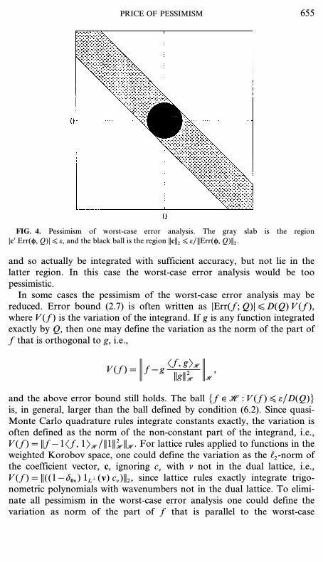
FIG. 4. Pessimism of worst-case error analysis. The gray slab is the region|cŒ Err(f, Q)| [ e, and the black ball is the region ||c||2 [ e/||Err(f, Q)||2.

and so actually be integrated with sufficient accuracy, but not lie in thelatter region. In this case the worst-case error analysis would be toopessimistic.In some cases the pessimism of the worst-case error analysis may be

reduced. Error bound (2.7) is often written as |Err(f; Q)| [ D(Q) V(f),where V(f) is the variation of the integrand. If g is any function integratedexactly by Q, then one may define the variation as the norm of the part off that is orthogonal to g, i.e.,

V(f)=>f−gOf, gPH

||g||2H>H

,

and the above error bound still holds. The ball {f ¥H : V(f) [ e/D(Q)}is, in general, larger than the ball defined by condition (6.2). Since quasi-Monte Carlo quadrature rules integrate constants exactly, the variation isoften defined as the norm of the non-constant part of the integrand, i.e.,V(f)=||f−1Of, 1PH/||1||2H ||H. For lattice rules applied to functions in theweighted Korobov space, one could define the variation as the a2-norm ofthe coefficient vector, c, ignoring cn with n not in the dual lattice, i.e.,V(f)=||((1−d0n) 1L+ (n) cn)||2, since lattice rules exactly integrate trigo-nometric polynomials with wavenumbers not in the dual lattice. To elimi-nate all pessimism in the worst-case error analysis one could define thevariation as norm of the part of f that is parallel to the worst-case


integrand, tQ, defined in (2.5), i.e., V(f)=|Of, tQPH |/||tQ ||. However, sucha definition of the variation would be difficult to apply in practice. In fact,it would be equivalent to knowing exactly the quadrature error, sinceOf, tQPH=Err(f; Q).Another way to reduce the pessimism in the worst-case analysis is to

redefine the space of integrands or the norm to make it more suitable forthe application at hand. In fact, the weights bj and bj were originallyintroduced in the definitions of the weighted Korobov and Sobolev spacesto study how much more effective quasi-Monte Carlo quadratures or arbi-trary quadratures are if the integrand depends less on the higher numberedcoordinates.The random-case quadrature analysis also has a pessimism problem.

Again, let e denote an error tolerance. By (3.1) the root mean square errorof a random quadrature rule Q for integrand f=cŒf ¥H will be no morethan this tolerance if

rmsQ ¥ Q

|Err(f; Q)|=`cŒLmQc [ e. (6.3)

This inequality defines an ellipsoidal ball in R., the space of coefficients c.However, Theorem 3.2 implies that integrands satisfying

||f||H=||c||2 [ e/e rand=e/`r(LmQ) (6.4)

will have root mean square error less than or equal to the tolerance e. Thisregion in R. corresponds to the largest spherical ball inscribed in the ellip-soid ball defined in (6.3). Figure 5 depicts the two regions defined in (6.3)and (6.4). It is clear that an integrand may lie in the former region, and soactually be integrated with sufficient accuracy, but not lie in the latterregion. In this case the random-case error analysis would be too pessi-mistic.The pessimism of the random-case error analysis may be eliminated in

principle by expanding the space of integrands or redefining the norm sothat the eigenvalues of LmQ are all the same. For example, starting from anoriginal Hilbert space H with ANOVA-consistent basis {fn}, one coulddefine another Hilbert space of integrands, H, using the basis defined as{fnr(L

mQ)/l

mQnn}. Since each new basis element is multiplied by a factor

r(LmQ)/lmQnn > 1, it follows thatH ı H. However, e rand for these two spaces

is the same. Moreover, for the new space H the ellipsoidal and sphericalballs in Fig. 5 coincide.One technical problem with defining a new Hilbert space in the manner

just mentioned is that the new basis may not satisfy (2.3). Moreover, eli-minating the pessimism in the random-case error analysis tends to widen


FIG. 5. Pessimism of random-case error analysis. The ellipsoidal ball is the region`cŒLmQc [ e, and the black spherical ball is the region ||c||2 [ e/`r(L

mQ) .

the gap between the worst-case and random-case error analyses. If theHilbert space of integrands is redefined to make the eigenvalues of LmQ allthe same, then eworst=`trace(LmQ) , becomes infinite, except in the case offinite-dimensional spaces of integrands.The average-case error analysis may be pessimistic if the matrix S is

chosen poorly. On the other hand, the average-case error analysis can bewildly optimistic. Since the quadrature rule in question usually integratessome basis elements extremely well, it is usually possible to choose S tomake eavg arbitrarily close to zero.

REFERENCES

1. M. Abrammowitz and I. A. Stegun (Eds.), ‘‘Handbook of Mathematical Functions withFormulas, Graphs and Mathematical Tables,’’ U. S. Government Printing Office,Washington, DC, 1964.

2. P. Acworth, M. Broadie, and P. Glasserman, A comparison of some Monte Carlo tech-niques for option pricing, in ‘‘Monte Carlo and Quasi-Monte Carlo Methods 1996’’(H. Niederreiter, P. Hellekalek, G. Larcher, and P. Zinterhof, Eds.), Lecture Notes inStatistics, Vol. 127, pp. 1–18, Springer-Verlag, New York 1996.

3. M. Aronszajn, Theory of reproducing kernels, Trans. Amer. Math. Soc. 68 (1950), 337–404.


4. R. E. Caflisch, W. Morokoff, and A. Owen, Valuation of mortgage backed securitiesusing Brownian bridges to reduce effective dimension, J. Comput. Finance 1 (1997), 27–46.

5. R. Cranley and T. N. L. Patterson, Randomization of number theoretic methods formultiple integration, SIAM J. Numer. Anal. 13 (1976), 904–914.

6. K. T. Fang and Y. Wang, ‘‘Number-Theoretic Methods in Statistics,’’ Chapman andHall, New York, 1994.

7. A. Genz, Comparison of methods for the computation of multivariate normal probabil-ities, Comput. Sci. Statist. 25 (1993), 400–405.

8. P. Hellekalek and G. Larcher, (Eds.), ‘‘Random and Quasi-Random Point Sets,’’ LectureNotes in Statistics, Vol. 138, Springer-Verlag, New York, 1998.

9. F. J. Hickernell, Lattice rules: How well do they measure up?, in ‘‘Random and Quasi-Random Point Sets’’ (P. Hellekalek and G. Larcher, Eds.), Lecture Notes in Statistics,Vol. 138, pp. 109–166, Springer-Verlag, New York, 1998.

10. F. J. Hickernell, Goodness-of-fit statistics, discrepancies and robust designs, Statist.Probab. Lett. 44 (1999), 73–78.

11. F. J. Hickernell, What affects the accuracy of quasi-Monte Carlo quadrature?, in ‘‘MonteCarlo and Quasi-Monte Carlo Methods 1998’’ (H. Niederreiter and J. Spanier, Eds.),pp. 16–55, Springer-Verlag, Berlin, 1999.

12. F. J. Hickernell, H. S. Hong, P. L’Ecuyer, and C. Lemieux, Extensible lattice sequencesfor quasi-Monte Carlo quadrature, SIAM J. Sci. Comput. 22 (2001), 1112–1138.

13. F. J. Hickernell and H. Wozniakowski, Integration and approximation in arbitrarydimensions, Adv. Comput. Math. 12 (2000), 25–58.

14. F. J. Hickernell and H. Wozniakowski, Tractability of multivariate integration forperiodic functions, J. Complexity 17 (2001), 660–682.

15. F. J. Hickernell and R. X. Yue, The mean square discrepancy of scrambled (t, s)-sequences, SIAM J. Numer. Anal. 38 (2001), 1089–1112.

16. B. D. Keister, Multidimensional quadrature algorithms, Comput. Phys. 10 (1996),119–122.

17. W. J. Morokoff and R. E. Caflisch, Quasi-Monte Carlo integration, J. Comput. Phys. 122(1995), 218–230.

18. H. Niederreiter, ‘‘Random Number Generation and Quasi-Monte Carlo Methods,’’CBMS-NSFRegionalConferenceSeries inAppliedMathematics, SIAM,Philadelphia, 1992.

19. H. Niederreiter and P. J.-S. Shiue, (Eds.), ‘‘Monte Carlo and Quasi-Monte Carlo Methodsin Scientific Computing,’’ Lecture Notes in Statistics, Vol. 106, Springer-Verlag, NewYork, 1995.

20. S. Ninomiya and S. Tezuka, Toward real-time pricing of complex financial derivatives,Appl. Math. Finance 3 (1996), 1–20.

21. E. Novak, ‘‘Deterministic and Stochastic Error Bounds in Numerical Analysis,’’ LecturesNotes in Mathematics, Vol. 1349, Springer-Verlag, Berlin, 1988.

22. E. Novak and H. Wozniakowski, When are integration and discrepancy tractable? in‘‘Foundations of Computational Mathematics’’ (R. Devore et al., Eds.), pp. 211–266,2001.

23. A. B. Owen, Randomly permuted (t, m, s)-nets and (t, s)-sequences, in ‘‘Monte Carlo andQuasi-Monte Carlo Methods in Scientific Computing’’ (H. Niederreiter and P. J.-S. Shiue,Eds.), Lecture Notes in Statistics, Vol. 106, pp. 299–317, Springer-Verlag, New York,1995.

24. A. B. Owen, Monte Carlo variance of scrambled equidistribution quadrature, SIAMJ. Number. Anal. 34 (1997), 1884–1910.

25. A. B. Owen and D. T. Tavella, Scrambled nets for value-at-risk calculations, in ‘‘VAR:Understanding and Applying Value-at-Risk’’ (S. Grayling, Ed.), pp. 257–273, RiskPublications, London, 1997.


26. A. Papageorgiou and J. F. Traub, Beating Monte Carlo, Risk 9(6) (1996), 63–65.27. A. Papageorgiou and J. F. Traub, Faster evaluation of multidimensional integrals,

Comput. in Phys. 11 (1997), 574–578.28. S. Paskov and J. Traub, Faster valuation of financial derivatives, J. Portfolio Manag. 22

(1995), 113–120.29. K. Ritter, ‘‘Average-Case Analysis of Numerical Problems,’’ Lecture Notes in Mathema-

tics, Vol. 1733, Springer-Verlag, Berlin, 2000.30. S. Saitoh, ‘‘Theory of Reproducing Kernels and Its Applications,’’ Longman Scientific &

Technical, Essex, England, 1988.31. I. H. Sloan and S. Joe, ‘‘Lattice Methods for Multiple Integration,’’ Oxford University

Press, Oxford, 1994.32. I. H. Sloan and H. Wozniakowski, When are quasi-Monte Carlo algorithms efficient for

high dimensional integrals, J. Complexity 14 (1998), 1–33.33. I. H. Sloan and H. Wozniakowski, Tractability of multivariate integration for weighted

Korobov classes, J. Complexity 17 (2001), 697–721.34. J. Spanier, Quasi-Monte Carlo methods for particle transport problems, in ‘‘Monte Carlo

and Quasi-Monte Carlo Methods in Scientific Computing’’ (H. Niederreiter and P. J.-S.Shiue, Eds.), Lecture Notes in Statistics, Vol. 106, pp. 121–148, Springer-Verlag, NewYork, 1995.

35. S. Tezuka, Financial applications of Monte Carlo and quasi-Monte Carlo methods, in‘‘Random and Quasi-Random Point Sets’’ (P. Hellekalek and G. Larcher, Eds.), LectureNotes in Statistics, Vol. 138, pp. 303–332, Springer-Verlag, New York, 1998.

36. J. F. Traub, G. W. Wasilkowski, and H. Wozniakowski, ‘‘Information-Based Complexity,’’Academic Press, Boston, 1988.

37. G. Wahba, ‘‘Spline Models for Observational Data,’’ SIAM, Philadelphia, 1990.38. X. Wang and F. J. Hickernell, Randomized Halton sequences, Math. Comput. Modelling

32 (2000), 887–899.


The Price of Pessimism for Multidimensional Quadrature

Documents

Transcript of The Price of Pessimism for Multidimensional Quadrature