The Predictive Power of the Yield Spread in Sub-Saharan and Northern Africa
50
1 The Predictive Power of the Yield Spread in Sub-Saharan and Northern Africa May 2008 By Oluwasegun Popoola
-
Upload
segunpopoola1849 -
Category
Documents
-
view
521 -
download
3
description
The predictive power of the yield spread has been widely studied and documented in the United States and a number of countries outside the United States. However, little or no studies have been conducted in Africa. This paper studies the predictive power of the yield spread and ascertains its usefulness for predicting real economic growth in Africa. It buttresses the predictive ability of the yield spread particularly in South Africa where the results suggest that the yield spread as a predictive indicator of future economic activities performs better at longer horizons.The paper further identifies the appropriate model for forecasting the yield spread in Morocco, Nigeria and South Africa.
Transcript of The Predictive Power of the Yield Spread in Sub-Saharan and Northern Africa
1
The Predictive Power of the
Yield Spread in Sub-Saharan and Northern Africa
May 2008
By Oluwasegun Popoola

2
Table of Contents
Abstract…………….………………………………………………………….……3
Section 1 Introduction……………………………………………………………...4
1.1 Background to the Study…………………………...4
1.2 Objectives of the Study..…………………………...6
1.3 Structure of the Study...…………………….……...6
Section 2 Literature Review and Theoretical Framework…………. ……………..7
2.1 Related Literature………………………..…………7
2.2 Theoretical Framework..…………………………....9
Section 3 Research Methodology, Empirical Analysis and Results……………...11
3.1 Data Description and Source(s)…………..….…….10
3.2 Predictive Power of the Yield Spread......................29
3.3 Forecasting Model Selection……............................44
Section 4 Summary of Research Findings, Recommendations and Conclusion…45
4.1 Summary of Research Findings……………………45
4.2 Conclusion..………………………………………..45
References…………………………………………………………………….…..48

3
Abstract
The predictive power of the yield spread has been widely studied and documented in the United States
and a number of countries outside the United States. However, little or no studies have been conducted in
Africa.
This paper studies the predictive power of the yield spread and ascertains its usefulness for predicting real
economic growth in Africa. It buttresses the predictive ability of the yield spread particularly in South
Africa where the results suggest that the yield spread as a predictive indicator of future economic
activities performs better at longer horizons.
The paper further identifies the appropriate model for forecasting the yield spread in Morocco, Nigeria
and South Africa.

4
SECTION 1
INTRODUCTION
1.1 Background to the Study
The use of financial variables to predict real economic activity only took a serious turn in the Nineties
when policymakers began to find alternative but more reliable ways of predicting economic conditions
having being previously been limited by the faulty macroeconomic models which are often characterized
by the lack of timely and accurate data and the complexity of the macroeconomic forecasting models.
The growing demand for such variables by policy makers fueled widening research into these variables
and their usefulness in predicting future economic conditions. One of such financial variables is the yield
spread, which is simply the difference between the long-term and short-term government instruments’
rates1.
Several studies have been conducted on the efficacy of the yield spread, which is often referred to as an
indicator of the future direction of the economy. Generally, a positive yield spread (i.e. higher long-term
interest rates than short-term rates) is associated with future economic expansion, while a negative yield
spread (i.e. lower long-term interest rates than short-term rates) is associated with future economic
contraction.
1 The widely used measure of the yield spread is the difference between the 10-year Treasury note and the 3-month
Treasury bill.

5
Harvey (1988) and several authors documented that there is information about future consumption and
output growth in the yield spread.
Bonser-Neal and Morley (1997) discovered that the predictive power of the yield spread is strongest in
Canada, Germany and the United States having taken the study of the efficacy of the yield spread further
by studying its implications in eleven OECD countries.
Perhaps, the closest semblance of a study of the yield spread and its predictive power in Africa was
conducted by Khomo and Aziakpono (2007) who both compared the efficacy of the yield curve and other
economic indicators as predictors of future economic activities (i.e. economic recessions and expansions)
in South Africa.
The seeming lack of studies on the yield spread in Africa is largely due to the nature of the African
monetary and financial markets which was largely seen as illiquid and sometimes not transparent because
of the level and size of government intervention and controls.
In addition, the institutional development frameworks for financial and monetary regulators and players
which were established about five decades ago in Sub-Saharan and Northern Africa (i.e. Morocco,
Nigeria and South Africa) only began to take strong roots in the last two decades. As a result, the use of
financial variables to forecast real economic activity was either absent or somewhat limited in most of the
countries studied.
This study is therefore is an attempt to ascertain the predictive power or otherwise of the yield spread in
three countries in Sub-Saharan and Northern Africa (i.e. Morocco, Nigeria and South Africa). The choice
of the countries was based on two criteria. First, only countries in the top five bracket of largest countries

6
in Africa in terms of real GDP were considered, Second, quarterly data on interest rates and (or) real
economic activity had to be available for at least the last ten years.
1.2 Objectives of the Study
The objectives of the study are:
Highlight the importance2 of the yield spread and determine the forecasting power
3 if any, of the
yield spread in Sub-Saharan and Northern Africa;
Appraise the theoretical underpinnings of the predictive capacity of the yield spread in Sub-
Saharan and Northern Africa; and
Consider the continued relevance of this financial variable in the light of constantly changing
economic conditions and circumstances.
1.3 Structure of the Study
The study covers the period 1963Q1 to 2006Q4. Section 2 contains a broad review of the existing and
relevant literature related to the study. A theoretical framework is also provided. Section 3 provides a
specification of the model, analysis of results obtained and the drawn generalizations from the findings.
Section 4 contains the summary of research findings, recommendations and conclusion.
2 Knowledge of the predictive ability of the yield spread enables businesses and policy makers to make better
forecasts of real economic activity in the light of unprecedented economic growth being recorded in Sub-Saharan
and Northern Africa in the last one decade. 3 As mentioned earlier, the yield spread is assumed to be a predictor of future economic conditions such as economic
expansion or contraction.

7
SECTION 2
RELATED LITERATURE AND THEORETICAL FRAMEWORK
2.1 Related Literature
Predictive role of the yield spread in industrial countries
Extensive studies on the predictive power of the yield spread and its predictive capacity began in the mid-
sixties when Kessel (1965) noted the existence of relationship between the yield curve and future real
economic activity. Ever since, researchers and analysts have continued to investigate the existence of a
relationship between these two economic variables.
In the late eighties and nineties, several studies including Harvey (1989) found that the yield spread
predicts real GDP growth in the United States. Stock and Watson (1989) empirically tested and
established a predictive relationship4 in macroeconomics that when the difference in yields between long
and short term interest rates in the United States is low or negative, future GDP growth tends to be slow
or negative. This view is also corroborated in Bernanke and Blinder (1992). Haubrich and Dombrosky
(1996) found that the yield spread is an excellent predictor of economic growth. Furthermore, Estrella and
Mishkin (1996), Dueker (1997) and Dotsey (1998) compare the yield curve with a few other variables5 as
a leading indicator of United States recessions and find generally supportive statistical evidence.
4 Recent findings however, indicate the relative weakness of the predictive power of yield curves and spreads to
forecast economic growth and future interest rates in the United States. For instance, the yield spread failed to
predict the 1990-1991 recession. Popoola (2007) 5 Alternative indicators are stock prices, stock returns, interest rates, dividend yields and exchange rates.

8
The early and mid-nineties also saw the emergence of a couple of studies on the predictive power of the
yield spread outside the United States. Estrella and Hardouvelis (1991) found that the yield spread
predicts real GDP growth in the United States and a number of European countries. Hu (1993), Caporale
(1994), Plosser and Rouwenhorst (1994) and Estrella and Mishkin (1995) all attempted to ascertain the
predictive power of the yield spread within and outside the United States. To the author’s best knowledge,
the most extensive multi-country analysis of the yield spread and its predictive capacity known to date
was conducted by Bonser-Neal and Morley (1997)6.
Predictive role of the yield spread in Africa
While extensive studies on the yield curve exist for the United States and a number of industrialized
countries, very little advancements have been made to study the yield curve and its predictive power in
other countries. Study on emerging economies let alone African countries are almost non-existent. This
view was buttressed by Mehl (2006).
Two works that specifically dwell on the yield spread and its predictive capacity relating to sub-Saharan
Africa were written by Mehl (2006) whose work was on the use of the slope of the yield curve to predict
domestic inflation and growth in South Africa among other emerging countries; while Khomo and
Aziakpono (2007) compared the efficacy of the yield curve and other economic indicators as predictors of
future economic activities (i.e. economic expansions or recessions) in South Africa.
Contribution
Interestingly, very few of the previous studies explored the possibility of appraising the theoretical
underpinnings of the predictive capacity of the yield spread in spite of the extensive literature available on
6 Bonser-Neal and Morley (1997) studied eleven OECD countries in their paper.

9
the subject matter. The only study known to the author was by Hamilton and Kim (2002) which attempted
to theoretically show evidence to buttress why the yield spread helps in forecasting the business cycle.
In addition, there has been no extensive work on the predictive capacity of the yield spread in African
countries except South Africa.
To the author’s best knowledge, this study is the first attempt to investigate and study the predictive
power of the yield spread in Morocco and Nigeria and provide an appropriate model for forecasting the
yield spread in Morocco, Nigeria and South Africa.
2.2 Theoretical Framework
The predictive capacity of the yield spread is embodied in an understanding of the relationship existing
between the yield curve, its movements and how it impacts economic conditions.7 A yield curve is the
graphical distribution of the yields of treasury securities with different maturities (i.e. 3-month, 6-month,
2, 3, 5, 10 and 20-year). The yield spread as described earlier is the difference between the long-term and
short-term government instruments’ rates. It is widely believed that the difference between the short and
long-term rates indicates the steepness or the slope of the yield curve.
A positive yield spread (i.e. long term rates are higher than short term rates; positively sloped yield curve)
is associated with a potential future increase in real economic activity while negative yield spread (i.e.
short term rates are higher than long term rates; negatively sloped or inverted yield curve) is associated
with a potential future decrease in real economic activity. Resultantly, the size of the yield spread
indicates the potential future increase or decline in real economic activity.
7 Guiding thoughts from Bonser-Neal and Morley (1997)

10
The following reasons have been adduced for the empirical relationship between the yield spread and its
predictive capacity:
The yield spread reflects the stance of monetary policy;
The yield spread reflects market expectations of future economic growth;
The yield spread reflects credit market conditions and in addition, reflects the changes in
expected inflation, fiscal situation and investors’ risk preferences.
Studies have consistently shown that all the theories listed above may have some merit. Estrella and
Hardovelis (1991) and Estrella and Mishkin (1995), for example, show that proxies for current monetary
policy do help forecast future real GDP growth; however, the inclusion of these proxies does not
eliminate the significance of the yield curve. These results suggest the yield curve reflects more than just
the effects of current monetary policy actions.

11
SECTION 3
RESEARCH METHODOLOGY, EMPIRICAL ANALYSIS AND
RESULTS
3.1 Data Description and Source(s)
The author studied three countries in Africa as previously documented in section one of the paper.
Real GDP is observed quarterly in South Africa and thus the sample is quarterly from 1963 through the
end of 2005 (i.e. 1963.01 to 2006.04). The author also obtained the 10-year government bond yield and 3-
month Treasury bill rate.
Quarterly real GDP for Morocco and Nigeria was unavailable. As a result, the author was unable to test
the predictive power of the yield spread. The author, however, obtained the quarterly 15-year Treasury
bond yield8 and 3-month Treasury bill rate for Morocco and deposit rate
9 and 3-month Treasury bill rate
for Nigeria in order to derive the yield spread.
All the data sets used for this study was sourced from the International Monetary Fund (IMF) data and
statistics electronic database.
8 15-year Treasury bond yield used in the absence of 10-year Treasury bond yield in Morocco.
9 The deposit rate was used as Nigeria discontinued the issuance of long term bonds only to have them re-introduced
about five years ago.

12
Figure 3.1 displays the time series plot of the annualized rate of growth of real GDP in South Africa over
the next four quarters which suggests that annualized growth rate in real GDP has been relatively unstable
over time.
Fig 3.1: Annualized Real GDP Growth Rates, 1963.01 – 2006.04 (South Africa)
-2
-1
0
1
2
3
4
5
65 70 75 80 85 90 95 00 05
GDP GROWTH RATE
Fig 3.2: Time series of T-bill rate and Government Bond Yield, 1963.01 – 2006.04 (South Africa)
0
4
8
12
16
20
24
65 70 75 80 85 90 95 00 05
TREASURY BILL RATE GOVERNMENT BOND YIELD

13
Fig 3.3: The Yield Spread and Real GDP growth rate, 1963.01 – 2006.04 (South Africa)
-6
-4
-2
0
2
4
6
8
65 70 75 80 85 90 95 00 05
GDP GROWTH RATE SPREAD
Fig 3.4: The Yield Spread, Real GDP growth rate and Periods of negative Real GDP growth rate, 1963.01 –
2006.04 (South Africa)
-6
-4
-2
0
2
4
6
8
65 70 75 80 85 90 95 00 05
GDP GROWTH RATE SPREAD
Figure 3.2 and 3.3 displays the time series of the T-bill rate and government bond yield rate and the yield
spread and real GDP respectively. Figure 3.4 displays the time series of the yield spread and real GDP.

14
The author observed that the yield spread declined into negative territory just before the real GDP turns
negative indicating the presence of predictive power in South Africa’s yield spread.
3.2 Predictive Power of the Yield Spread
The author followed the standard regression methodology adopted in previous studies, such as Estrella
and Hardouvelis (1991), Estrella and Mishkin (1997) and Bonser-Neal and Morley (1997).
Model Specification
(ΔY) t, t+k = α + β*spreadt + error,
Where ΔY is the change in real economic activity and defined as the annualized growth rate in real GDP.
The subscript k denotes the forecasting horizon in quarters and the spread is defined as the difference
between the long-term and short-term rates.
Results
The results reported in Table 3.1 indicates the yield spread explains roughly between 5% and 7% of the
variation in the following period’s real GDP (i.e. t + k). In addition, the results seem to support the
findings, in Khomo and Aziakpono (2007) that the yield spread as a predictive indicator of future
economic activities performs better at longer horizons compared to other leading indicators in South
Africa.

15
Table 3.1: Explanatory Power of the Yield Spread for Real GDP
Forecasting
Horizon;
Explanatory Power of the
Yield Spread for Real GDP
k Quarters
Ahead
1 5.66
2 6.10
3 6.23
4 6.27
5 6.27
6 6.27
7 6.30
8 6.37
12 6.47
16 6.60
20 6.74
3.3 Forecasting Model Selection
The author applied a number of models including trend, seasonality and ARMA regression models to
choose the best model to forecast yield spread from January to December 2006.

16
Trend Regression Model
Linear Trend Model
Yt = o + 1Timet + t
Table 3.2: Linear Trend Regression (South Africa)
Table 3.3: Linear Trend Regression (Morocco)
Dependent Variable: SPREAD
Method: Least Squares
Date: 05/04/08 Time: 23:29
Sample: 1963Q1 2005Q4
Included observations: 172
Variable Coefficient Std. Error t-Statistic Prob.
C 2.854042 0.357074 7.992849 0.0000
TIME -0.011156 0.003612 -3.089045 0.0023
R-squared 0.053147 Mean dependent var 1.900193
Adjusted R-squared 0.047578 S.D. dependent var 2.409735
S.E. of regression 2.351711 Akaike info criterion 4.559723
Sum squared resid 940.1927 Schwarz criterion 4.596322
Log likelihood -390.1362 F-statistic 9.542199
Durbin-Watson stat 0.159212 Prob(F-statistic) 0.002346
Dependent Variable: SPREAD
Method: Least Squares
Date: 05/06/08 Time: 01:18
Sample: 1998Q1 2005Q4
Included observations: 32
Variable Coefficient Std. Error t-Statistic Prob.
C 1.442309 0.183345 7.866632 0.0000
TIME 0.027815 0.010162 2.737035 0.0103
R-squared 0.199816 Mean dependent var 1.873437
Adjusted R-squared 0.173143 S.D. dependent var 0.583715
S.E. of regression 0.530782 Akaike info criterion 1.631531
Sum squared resid 8.451888 Schwarz criterion 1.723139
Log likelihood -24.10450 F-statistic 7.491363
Durbin-Watson stat 0.488715 Prob(F-statistic) 0.010319

17
Table 3.4: Linear Trend Regression (Nigeria)
Quadratic Trend Model
Yt = o + 1Timet + 2Timet2 + t
Table 3.5: Quadratic Trend Regression (South Africa)
Dependent Variable: SPREAD
Method: Least Squares
Date: 05/06/08 Time: 02:54
Sample: 1992Q1 2005Q4
Included observations: 56
Variable Coefficient Std. Error t-Statistic Prob.
C 1.250543 0.690317 1.811548 0.0756
TIME 0.000645 0.021641 0.029795 0.9763
R-squared 0.000016 Mean dependent var 1.268275
Adjusted R-squared -0.018502 S.D. dependent var 2.593718
S.E. of regression 2.617602 Akaike info criterion 4.797456
Sum squared resid 369.9995 Schwarz criterion 4.869790
Log likelihood -132.3288 F-statistic 0.000888
Durbin-Watson stat 0.584429 Prob(F-statistic) 0.976341
Dependent Variable: SPREAD
Method: Least Squares
Date: 05/04/08 Time: 23:36
Sample: 1963Q1 2005Q4
Included observations: 172
Variable Coefficient Std. Error t-Statistic Prob.
C 2.480436 0.531913 4.663240 0.0000
TIME 0.002030 0.014373 0.141239 0.8878
TIME^2 -7.71E-05 8.14E-05 -0.947883 0.3445
R-squared 0.058155 Mean dependent var 1.900193
Adjusted R-squared 0.047009 S.D. dependent var 2.409735
S.E. of regression 2.352414 Akaike info criterion 4.566049
Sum squared resid 935.2207 Schwarz criterion 4.620947
Log likelihood -389.6802 F-statistic 5.217491
Durbin-Watson stat 0.160069 Prob(F-statistic) 0.006328

18
Table 3.6: Quadratic Trend Regression (Morocco)
Table 3.7: Quadratic Trend Regression (Nigeria)
Dependent Variable: SPREAD
Method: Least Squares
Date: 05/06/08 Time: 01:19
Sample: 1998Q1 2005Q4
Included observations: 32
Variable Coefficient Std. Error t-Statistic Prob.
C 1.028893 0.247380 4.159157 0.0003
TIME 0.110498 0.036936 2.991644 0.0056
TIME^2 -0.002667 0.001151 -2.316430 0.0278
R-squared 0.324756 Mean dependent var 1.873437
Adjusted R-squared 0.278187 S.D. dependent var 0.583715
S.E. of regression 0.495922 Akaike info criterion 1.524263
Sum squared resid 7.132218 Schwarz criterion 1.661676
Log likelihood -21.38822 F-statistic 6.973708
Durbin-Watson stat 0.577224 Prob(F-statistic) 0.003367
Dependent Variable: SPREAD
Method: Least Squares
Date: 05/06/08 Time: 02:54
Sample: 1992Q1 2005Q4
Included observations: 56
Variable Coefficient Std. Error t-Statistic Prob.
C -2.035820 0.815493 -2.496430 0.0157
TIME 0.365796 0.068563 5.335170 0.0000
TIME^2 -0.006639 0.001206 -5.506504 0.0000
R-squared 0.363921 Mean dependent var 1.268275
Adjusted R-squared 0.339918 S.D. dependent var 2.593718
S.E. of regression 2.107278 Akaike info criterion 4.380754
Sum squared resid 235.3529 Schwarz criterion 4.489255
Log likelihood -119.6611 F-statistic 15.16148
Durbin-Watson stat 0.915792 Prob(F-statistic) 0.000006

19
Exponential Trend Model
Yt = oe1Timet
+ t
Table 3.8: Exponential Trend Regression (South Africa)
Table 3.9: Exponential Trend Regression (Morocco)
Dependent Variable: SPREAD
Method: Least Squares
Date: 05/06/08 Time: 01:21
Sample: 1998Q1 2005Q4
Included observations: 32
Convergence achieved after 9 iterations
SPREAD=C(1)*EXP(C(2)*TIME) Coefficient Std. Error t-Statistic Prob.
C(1) 1.511348 0.167015 9.049159 0.0000
C(2) 0.013417 0.005542 2.420939 0.0217
R-squared 0.181001 Mean dependent var 1.873437
Adjusted R-squared 0.153701 S.D. dependent var 0.583715
S.E. of regression 0.536986 Akaike info criterion 1.654772
Sum squared resid 8.650618 Schwarz criterion 1.746380
Log likelihood -24.47635 Durbin-Watson stat 0.477824
Dependent Variable: SPREAD
Method: Least Squares
Date: 05/04/08 Time: 23:40
Sample: 1963Q1 2005Q4
Included observations: 172
Convergence achieved after 6 iterations
SPREAD=C(1)*EXP(C(2)*TIME) Coefficient Std. Error t-Statistic Prob.
C(1) 2.893209 0.438064 6.604528 0.0000
C(2) -0.005262 0.001986 -2.649734 0.0088
R-squared 0.048053 Mean dependent var 1.900193
Adjusted R-squared 0.042454 S.D. dependent var 2.409735
S.E. of regression 2.358029 Akaike info criterion 4.565089
Sum squared resid 945.2509 Schwarz criterion 4.601688
Log likelihood -390.5976 Durbin-Watson stat 0.158361

20
Table 3.10: Exponential Trend Regression (Nigeria)
Table 3.11: Comparing AIC and SIC (South Africa)
Trend AIC SIC
Linear 4.5377 4.5737
Quadratic 4.5433 4.5974
Exponential 4.5439 4.5800
Table 3.12: Comparing AIC and SIC (Morocco)
Trend AIC SIC
Linear 1.6315 1.7231
Quadratic 1.5242 1.6617
Exponential 1.6548 1.7464
Dependent Variable: SPREAD
Method: Least Squares
Date: 05/06/08 Time: 03:03
Sample: 1992Q1 2005Q4
Included observations: 56
Convergence achieved after 6 iterations
SPREAD=C(1)*EXP(C(2)*TIME) Coefficient Std. Error t-Statistic Prob.
C(1) -4.67E-13 5.30E-12 -0.088176 0.9301
C(2) 0.702880 2.95E-06 238064.3 0.0000
R-squared
-2959146.6
08949 Mean dependent var 1.268275
Adjusted R-squared
-3013945.6
38744 S.D. dependent var 2.593718
S.E. of regression 4502.882 Akaike info criterion 19.69788
Sum squared resid 1.09E+09 Schwarz criterion 19.77022
Log likelihood -549.5407 Durbin-Watson stat 0.255009

21
Table 3.13: Comparing AIC and SIC (Nigeria)
Trend AIC SIC
Linear 4.7975 4.8698
Quadratic 4.3808 4.4892
Exponential 19.6979 19.7702
Having considered the three models (i.e. linear, quadratic and exponential), we adopt the linear model for
South Africa and the quadratic model for Morocco and Nigeria10
.
A cursory look at the regression statistics produced by the linear trend model for South Africa and
quadratic model for Morocco and Nigeria reveal the following:
Linear Trend Model – South Africa
The linear term is significant11
.
R2
indicates that the trend is only responsible for about 5.3% of the variation in the yield
spread.
A Durbin-Watson statistic of 0.159 indicates the presence of positive serial correlation.
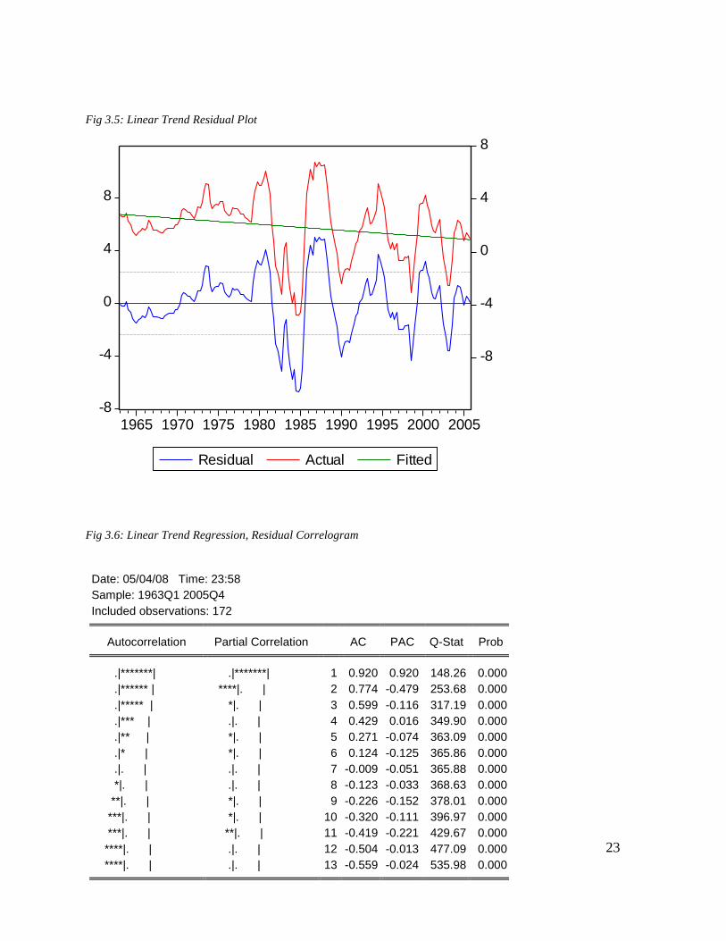
The linear trend regression residual plot in figure 3.5 reveals that the fitted trend remains relatively stable
throughout. As a result, it is difficult to notice any obvious seasonality or cyclical patterns.
Quadratic Model – Morocco
The linear and quadratic terms are significant.
10
The model with the lowest SIC and AIC for each country is selected in this instance. 11
Except otherwise stated, test of significance is at the 95% confidence interval.

22
R2 indicates that the trend is only responsible for about 32% of the variation in the yield
spread.
A Durbin-Watson statistic of 0.5772 indicates the presence of positive serial correlation.
The fitted trend remains stable throughout as can be seen from the quadratic trend regression residual plot
in figure 3.7. As a result, it is difficult to notice any obvious seasonality or cyclical patterns.
Quadratic Model – Nigeria
The linear and quadratic terms are significant.
R2 indicates that the trend is only responsible for about 36% of the variation in the yield
spread.
A Durbin-Watson statistic of 0.9158 indicates the presence of positive serial correlation.
The fitted trend remains stable as can be seen from the quadratic trend regression residual plot in figure
3.9. As a result, it is difficult to notice any obvious seasonality or cyclical patterns.
The residual correlograms and its graphs (i.e. figure 3.6, 3.7 and 3.8) reveal the residual sample
autocorrelation and partial autocorrelation function has spikes in the 1st, 2
nd, 9
th and 11
th lags for South
Africa; 1st and 2
nd lags for Morocco and 1
st, 2
nd, 9
th and 11
th lags for Nigeria. Additionally, it can been
seen that the Ljung-Box statistic rejects the white noise null hypothesis even at very small, non-seasonal
displacements which means there is still some useful information contained in the residuals which can be
extracted.
23
Fig 3.5: Linear Trend Residual Plot
-8
-4
0
4
8
-8
-4
0
4
8
1965 1970 1975 1980 1985 1990 1995 2000 2005
Residual Actual Fitted
Fig 3.6: Linear Trend Regression, Residual Correlogram
Date: 05/04/08 Time: 23:58
Sample: 1963Q1 2005Q4
Included observations: 172
Autocorrelation Partial Correlation AC PAC Q-Stat Prob
.|*******| .|*******| 1 0.920 0.920 148.26 0.000
.|****** | ****|. | 2 0.774 -0.479 253.68 0.000
.|***** | *|. | 3 0.599 -0.116 317.19 0.000
.|*** | .|. | 4 0.429 0.016 349.90 0.000
.|** | *|. | 5 0.271 -0.074 363.09 0.000
.|* | *|. | 6 0.124 -0.125 365.86 0.000
.|. | .|. | 7 -0.009 -0.051 365.88 0.000
*|. | .|. | 8 -0.123 -0.033 368.63 0.000
**|. | *|. | 9 -0.226 -0.152 378.01 0.000
***|. | *|. | 10 -0.320 -0.111 396.97 0.000
***|. | **|. | 11 -0.419 -0.221 429.67 0.000
****|. | .|. | 12 -0.504 -0.013 477.09 0.000
****|. | .|. | 13 -0.559 -0.024 535.98 0.000

24
Fig 3.7: Quadratic Trend Residual Plot (Morocco)
-2.0
-1.5
-1.0
-0.5
0.0
0.5
1.0
0
1
2
3
1998 1999 2000 2001 2002 2003 2004 2005
Residual Actual Fitted
Fig 3.8: Quadratic Trend Regression, Residual Correlogram (Morocco)
Date: 05/06/08 Time: 01:31
Sample: 1998Q1 2005Q4
Included observations: 32
Autocorrelation Partial Correlation AC PAC Q-Stat Prob
. |***** | . |***** | 1 0.693 0.693 16.871 0.000
. |**. | ****| . | 2 0.224 -0.493 18.699 0.000
. *| . | . |* . | 3 -0.069 0.103 18.878 0.000
.**| . | .**| . | 4 -0.241 -0.264 21.140 0.000
.**| . | . | . | 5 -0.308 0.010 24.965 0.000

25
Fig 3.9: Quadratic Trend Residual Plot
-8
-4
0
4
8
-8
-4
0
4
8
92 93 94 95 96 97 98 99 00 01 02 03 04 05
Residual Actual Fitted
Fig 3.10: Quadratic Trend Regression, Residual Correlogram
Date: 05/06/08 Time: 03:10
Sample: 1992Q1 2005Q4
Included observations: 56
Autocorrelation Partial Correlation AC PAC Q-Stat Prob
. |**** | . |**** | 1 0.532 0.532 16.734 0.000
. |*. | .*| . | 2 0.165 -0.165 18.370 0.000
. | . | . | . | 3 0.044 0.043 18.490 0.000
. | . | . | . | 4 0.009 -0.014 18.495 0.001
. | . | . | . | 5 0.002 0.005 18.496 0.002
. | . | . | . | 6 -0.000 -0.002 18.496 0.005
. | . | . | . | 7 0.043 0.064 18.619 0.009
. | . | .*| . | 8 0.013 -0.061 18.630 0.017
.*| . | .*| . | 9 -0.064 -0.066 18.911 0.026
**| . | .*| . | 10 -0.197 -0.178 21.661 0.017
**| . | . | . | 11 -0.211 -0.018 24.862 0.010
.*| . | . | . | 12 -0.153 -0.035 26.601 0.009
.*| . | . | . | 13 -0.059 0.048 26.866 0.013

26
Modeling Seasonality
In order to test for seasonality, the author generated four dummy variables for the quarters in a year and
performed a regression using both the linear trend and seasonal dummies in the case of South Africa and
quadratic trend and seasonal dummies in the case of Morocco and Nigeria.
The results of the regression on seasonal dummies for South Afirca, Moroco and Nigeria are shown in
Tables 3.14, 3.15 and 3.16 respectively. The seasonal dummy model is
4
Yt = i Dit + t i=1
Table 3.14: Seasonal Dummy Variable Model (South Africa)
Dependent Variable: SPREAD
Method: Least Squares
Date: 05/05/08 Time: 00:38
Sample: 1963Q1 2005Q4
Included observations: 172
Variable Coefficient Std. Error t-Statistic Prob.
D1 1.811237 0.370623 4.887012 0.0000
D2 1.975157 0.370623 5.329295 0.0000
D3 1.876001 0.370623 5.061756 0.0000
D4 1.938377 0.370623 5.230057 0.0000
R-squared 0.000675 Mean dependent var 1.900193
Adjusted R-squared -0.017171 S.D. dependent var 2.409735
S.E. of regression 2.430335 Akaike info criterion 4.636916
Sum squared resid 992.2965 Schwarz criterion 4.710114
Log likelihood -394.7748 Durbin-Watson stat 0.147940

27
Table 3.15: Seasonal Dummy Variable Model (Morocco)
Table 3.16: Seasonal Dummy Variable Model (Nigeria)
Dependent Variable: SPREAD
Method: Least Squares
Date: 05/06/08 Time: 03:13
Sample: 1992Q1 2005Q4
Included observations: 56
Variable Coefficient Std. Error t-Statistic Prob.
D1 1.697393 0.703108 2.414127 0.0193
D2 1.585945 0.703108 2.255619 0.0283
D3 0.613574 0.703108 0.872658 0.3869
D4 1.176188 0.703108 1.672840 0.1004
R-squared 0.027325 Mean dependent var 1.268275
Adjusted R-squared -0.028791 S.D. dependent var 2.593718
S.E. of regression 2.630791 Akaike info criterion 4.841195
Sum squared resid 359.8952 Schwarz criterion 4.985863
Log likelihood -131.5535 Durbin-Watson stat 0.545425
Dependent Variable: SPREAD
Method: Least Squares
Date: 05/06/08 Time: 01:36
Sample: 1998Q1 2005Q4
Included observations: 32
Variable Coefficient Std. Error t-Statistic Prob.
D1 1.974584 0.215272 9.172499 0.0000
D2 1.917082 0.215272 8.905389 0.0000
D3 1.793750 0.215272 8.332475 0.0000
D4 1.808333 0.215272 8.400215 0.0000
R-squared 0.017211 Mean dependent var 1.873437
Adjusted R-squared -0.088087 S.D. dependent var 0.583715
S.E. of regression 0.608882 Akaike info criterion 1.962083
Sum squared resid 10.38063 Schwarz criterion 2.145300
Log likelihood -27.39333 Durbin-Watson stat 0.351156

28
The dummies account for less than 1 percent of the variation in the yield spread for the three countries. As
a result, the author considered the linear trend model and the dummies below for South Africa and the
quadratic trend model and dummies below for Morocco and South Africa.
Yt = o + 1Timet + i Dit + t South Africa
Yt = o + 1Timet + 2Timet2 + i Dit + t Morocco and Nigeria
i=1
Table 3.17: Shows the Linear Trend and Seasonal Dummy Variable Regression Results (South Africa)
Dependent Variable: SPREAD
Method: Least Squares
Date: 05/05/08 Time: 00:44
Sample: 1963Q1 2005Q4
Included observations: 172
Variable Coefficient Std. Error t-Statistic Prob.
TIME -0.011176 0.003643 -3.067731 0.0025
D1 2.750030 0.473774 5.804524 0.0000
D2 2.925126 0.476135 6.143482 0.0000
D3 2.837146 0.478512 5.929098 0.0000
D4 2.910699 0.480906 6.052537 0.0000
R-squared 0.053985 Mean dependent var 1.900193
Adjusted R-squared 0.031326 S.D. dependent var 2.409735
S.E. of regression 2.371690 Akaike info criterion 4.593722
Sum squared resid 939.3606 Schwarz criterion 4.685219
Log likelihood -390.0601 Durbin-Watson stat 0.156185

29
Table 3.18: Shows the Quadratic Trend and Seasonal Dummy Variable Regression Results (Morocco)
Table 3.19: Shows the Quadratic Trend and Seasonal Dummy Variable Regression Results (Nigeria)
Dependent Variable: SPREAD
Method: Least Squares
Date: 05/06/08 Time: 01:38
Sample: 1998Q1 2005Q4
Included observations: 32
Variable Coefficient Std. Error t-Statistic Prob.
TIME 0.111948 0.038035 2.943313 0.0068
TIME^2 -0.002671 0.001185 -2.253588 0.0329
D1 1.155124 0.291318 3.965169 0.0005
D2 1.063127 0.297569 3.572709 0.0014
D3 0.910640 0.302575 3.009637 0.0057
D4 0.901410 0.306396 2.941973 0.0068
R-squared 0.358772 Mean dependent var 1.873437
Adjusted R-squared 0.235459 S.D. dependent var 0.583715
S.E. of regression 0.510389 Akaike info criterion 1.660074
Sum squared resid 6.772923 Schwarz criterion 1.934899
Log likelihood -20.56118 Durbin-Watson stat 0.535745
Dependent Variable: SPREAD
Method: Least Squares
Date: 05/06/08 Time: 03:15
Sample: 1992Q1 2005Q4
Included observations: 56
Variable Coefficient Std. Error t-Statistic Prob.
TIME 0.367195 0.069042 5.318423 0.0000
TIME^2 -0.006642 0.001214 -5.471797 0.0000
D1 -1.632462 0.943469 -1.730276 0.0897
D2 -1.759062 0.953645 -1.844568 0.0710
D3 -2.733301 0.962518 -2.839738 0.0065
D4 -2.159269 0.970127 -2.225759 0.0306
R-squared 0.391712 Mean dependent var 1.268275
Adjusted R-squared 0.330883 S.D. dependent var 2.593718
S.E. of regression 2.121650 Akaike info criterion 4.443223
Sum squared resid 225.0700 Schwarz criterion 4.660225
Log likelihood -118.4102 Durbin-Watson stat 0.867988

30
From the foregoing results, the inclusion of the dummy variables provides little or no explanation for the
variation in the yield spread at least in the case of South Africa. The author therefore excludes the dummy
variables from the forecast model for South Africa but includes the dummy variables in the forecast
models for Morocco and Nigeria.
Incorporating the ARMA Model
AR (p) model
yt = c + 1yt-1 + 2yt-2 + …….. + pyt-p + t
MA (q) model
yt = + t + 1 t-1 + 2 t-2 + ………. + q t-q
Tables 3.20 to 3.26 provide the AIC and SIC estimates for various AR and MA processes.
Table 3.20: AIC Values, ARMA Models (South Africa)
MA Order
0 1 2 3 4
0 3.836832 3.213445 2.847858 2.666828
AR Order 1 2.696736 2.535904 2.478719 2.481130 2.492796
2 2.473483 2.479649 2.486647 2.498621 2.476628
3 2.484050 2.462456 2.474071 2.484896 2.495511
4 2.496814 2.477522 2.486658 2.511902 2.507652
Table 3.21: SIC Values, ARMA Models (South Africa)
MA Order
0 1 2 3 4
0 3.873431 3.268343 2.921056 2.758325
AR Order 1 2.733481 2.591021 2.552208 2.572992 2.603030
2 2.528821 2.553432 2.578876 2.609296 2.605750
3 2.558131 2.555057 2.585191 2.614537 2.643672
4 2.589789 2.589092 2.616823 2.660663 2.675007

31
Table 3.22: AIC Values, ARMA Models (Morocco)
MA Order
0 1 2 3 4
0 4.107412 4.096161 4.127168 4.161448
AR Order 1 4.102316 4.108774 3.975994 4.101645 4.125594
2 4.125950 3.986706 3.976569 3.991413 3.906611
3 4.172017 4.018662 4.131278 4.082619 4.123159
4 4.231887 4.038840 4.002267 4.061713 3.984842
Table 3.23: SIC Values, ARMA Models (Morocco)
MA Order
0 1 2 3 4
0 4.360581 4.385497 4.452671 4.523118
AR Order 1 4.357795 4.400750 4.304467 4.466615 4.527061
2 4.420615 4.318203 4.344900 4.396576 4.348607
3 4.506595 4.390415 4.540207 4.528722 4.606439
4 4.607126 4.451603 4.452554 4.549524 4.510177
Table 3.24: AIC Values, ARMA Models (Nigeria)
MA Order
0 1 2 3 4
0 4.107412 4.096161 4.127168 4.161448
AR Order 1 4.102316 4.108774 3.975994 4.101645 4.125594
2 4.125950 3.986706 3.976569 3.991413 3.906611
3 4.172017 4.018662 4.131278 4.082619 4.123159
4 4.231887 4.038840 4.002267 4.061713 3.984842
Table 3.25: SIC Values, ARMA Models (Nigeria)
MA Order
0 1 2 3 4
0 4.360581 4.385497 4.452671 4.523118
AR Order 1 4.357795 4.400750 4.304467 4.466615 4.527061
2 4.420615 4.318203 4.344900 4.396576 4.348607
3 4.506595 4.390415 4.540207 4.528722 4.606439
4 4.607126 4.451603 4.452554 4.549524 4.510177

32
Based on the results from the AIC and SIC, we select the ARMA (2, 0) for South Africa; ARMA (3, 2)
for Morocco and ARMA (1, 2) for Nigeria.
This suggests that the best model to regress yield spread is the ARMA (2, 0) model inclusive of the linear
trend but excluding the seasonal dummies for South Africa; ARMA (3, 2) and ARMA (1, 2) model
inclusive of the quadratic trend and seasonal dummies for Morocco and Nigeria respectively.
As such, the new model adopted is:
Yt = o + 1Timet + 2yt-2 + t South Africa i=1
Yt = o + 1Timet + 2Timet2 + i Dit + 2yt-2 + t Morocco and Nigeria
i=1
Table 3.26: Linear Trend Regression and ARMA (2, 0) Disturbances (South Africa)
Dependent Variable: SPREAD
Method: Least Squares
Date: 05/05/08 Time: 05:22
Sample (adjusted): 1963Q3 2005Q4
Included observations: 170 after adjustments
Convergence achieved after 4 iterations
Variable Coefficient Std. Error t-Statistic Prob.
TIME 0.012936 0.007089 1.824890 0.0698
AR(1) 1.375742 0.068624 20.04747 0.0000
AR(2) -0.461797 0.068463 -6.745181 0.0000
R-squared 0.885042 Mean dependent var 1.890489
Adjusted R-squared 0.883665 S.D. dependent var 2.422260
S.E. of regression 0.826181 Akaike info criterion 2.473483
Sum squared resid 113.9900 Schwarz criterion 2.528821
Log likelihood -207.2461 Durbin-Watson stat 2.074602
Inverted AR Roots .79 .58

33
Table 3.27: Quadratic Trend Regression, Seasonal Dummies and ARMA (3, 2) Disturbances (Morocco)
Dependent Variable: SPREAD
Method: Least Squares
Date: 05/06/08 Time: 02:14
Sample (adjusted): 1998Q4 2005Q4
Included observations: 29 after adjustments
Convergence achieved after 108 iterations
Backcast: OFF (Roots of MA process too large)
Variable Coefficient Std. Error t-Statistic Prob.
TIME 0.226916 0.068170 3.328678 0.0037
TIME^2 -0.005621 0.001904 -2.951913 0.0085
D1 0.207156 0.525318 0.394343 0.6980
D2 0.116748 0.545711 0.213937 0.8330
D3 -0.099565 0.552776 -0.180118 0.8591
D4 0.001071 0.536030 0.001999 0.9984
AR(1) 0.940373 0.233439 4.028352 0.0008
AR(2) -0.070506 0.354592 -0.198838 0.8446
AR(3) -0.240043 0.231763 -1.035722 0.3140
MA(1) -0.099211 0.613869 -0.161617 0.8734
MA(2) -2.035910 0.656769 -3.099885 0.0062
R-squared 0.964129 Mean dependent var 1.897816
Adjusted R-squared 0.944201 S.D. dependent var 0.608116
S.E. of regression 0.143649 Akaike info criterion -0.761197
Sum squared resid 0.371428 Schwarz criterion -0.242568
Log likelihood 22.03736 Durbin-Watson stat 2.197198
Inverted AR Roots .67-.39i .67+.39i -.40
Inverted MA Roots 1.48 -1.38
Estimated MA process is noninvertible

34
Table 3.28: Quadratic Trend Regression, Seasonal Dummies and ARMA (1, 2) Disturbances (Nigeria)
Table 3.26 shows the regression results from the linear trend and ARMA (2, 0) model. Each of the
coefficients is significant. R2 for the model is now 88.37 percent. The Durbin-Watson statistic is now very
acceptable and the standard error of the regression is now reduced to 0.8262.
Table 3.27 shows the regression results from the quadratic trend and ARMA (3, 2) model. In spite of the
fact that some of the coefficients are insignificant, the R2
for the model is now 96 percent. The Durbin-
Watson statistic is now very acceptable and the standard error of the regression is now reduced to 0.1436.
Dependent Variable: SPREAD
Method: Least Squares
Date: 05/06/08 Time: 04:09
Sample (adjusted): 1992Q2 2005Q4
Included observations: 55 after adjustments
Convergence achieved after 20 iterations
Backcast: 1991Q4 1992Q1
Variable Coefficient Std. Error t-Statistic Prob.
TIME 0.791903 0.204280 3.876562 0.0003
TIME^2 -0.012240 0.002623 -4.665945 0.0000
D1 -8.977489 3.965062 -2.264148 0.0283
D2 -9.143115 4.000570 -2.285453 0.0269
D3 -10.05746 3.972891 -2.531523 0.0148
D4 -9.410579 3.927692 -2.395956 0.0207
AR(1) 0.850948 0.063813 13.33502 0.0000
MA(1) -0.441986 0.124828 -3.540754 0.0009
MA(2) -0.553947 0.127364 -4.349324 0.0001
R-squared 0.664313 Mean dependent var 1.289516
Adjusted R-squared 0.605933 S.D. dependent var 2.612704
S.E. of regression 1.640118 Akaike info criterion 3.975994
Sum squared resid 123.7394 Schwarz criterion 4.304467
Log likelihood -100.3398 Durbin-Watson stat 1.882480
Inverted AR Roots .85
Inverted MA Roots 1.00 -.56

35
Table 3.28 shows the regression results from the Linear Trend and ARMA (1, 2) model. Each of the
coefficients, except for the linear trend coefficients is significant. Even though the linear trend coefficient
is now insignificant, the adjusted R2
for the model is now 88.37 percent. The Durbin-Watson statistic is
now very acceptable and the standard error of the regression is now reduced to 0.8262.
Figures 3.11, 3.13 and 3.15 shows the residual plots for the selected models for South Africa, Morocco
and Nigeria, which looks like white noise and this is also confirmed by the residual correlograms (figures
3.12, 3.14 and 3.16). The sample autocorrelations and partial autocorrelations show no more patterns and
are mostly within the standard error bounds. Each of the Q-stats is insignificant thereby providing
evidence that white noise does exist. As such, the model is able to capture the elements explaining the
variation in the yield spread.
Fig 3.11: Linear Trend Regression and ARMA (2, 0) Residual Plot
-4
-2
0
2
4
-8
-4
0
4
8
1965 1970 1975 1980 1985 1990 1995 2000 2005
Residual Actual Fitted

36
Fig 3.12: Linear Trend Regression and ARMA (2, 0), Residual Correlogram
Date: 05/05/08 Time: 06:32
Sample: 1963Q3 2005Q4
Included observations: 170 Q-statistic
probabilities adjusted for 2 ARMA
term(s)
Autocorrelation Partial Correlation AC PAC Q-Stat Prob
.|. | .|. | 1 -0.043 -0.043 0.3169
.|* | .|* | 2 0.081 0.079 1.4477
.|. | .|. | 3 -0.048 -0.042 1.8538 0.173
.|. | .|. | 4 -0.020 -0.030 1.9249 0.382
.|. | .|. | 5 0.038 0.044 2.1795 0.536
.|. | .|. | 6 0.017 0.022 2.2300 0.694
*|. | *|. | 7 -0.078 -0.086 3.3172 0.651
.|. | .|. | 8 0.048 0.043 3.7245 0.714
*|. | *|. | 9 -0.103 -0.084 5.6338 0.583
.|* | .|* | 10 0.146 0.128 9.5331 0.299
.|. | .|. | 11 -0.048 -0.029 9.9597 0.354
*|. | *|. | 12 -0.077 -0.104 11.050 0.354
*|. | *|. | 13 -0.142 -0.140 14.794 0.192

37
Fig 3.13: Quadratic Trend, Seasonality and ARMA (3, 2) Regression Residual Plot (Morocco)
-.4
-.3
-.2
-.1
.0
.1
.2
0
1
2
3
1999 2000 2001 2002 2003 2004 2005
Residual Actual Fitted
Fig 3.14: Quadratic Trend, Seasonality and ARMA (3, 2) Regression, Residual Correlogram (Morocco)
Date: 05/06/08 Time: 02:16
Sample: 1998Q4 2005Q4
Included observations: 29 Q-statistic
probabilities adjusted for 5 ARMA
term(s)
Autocorrelation Partial Correlation AC PAC Q-Stat Prob
. *| . | . *| . | 1 -0.132 -0.132 0.5622
.**| . | .**| . | 2 -0.265 -0.288 2.9062
. *| . | . *| . | 3 -0.083 -0.184 3.1432
. *| . | .**| . | 4 -0.074 -0.232 3.3412
. |* . | . *| . | 5 0.078 -0.082 3.5716

38
Fig 3.15: Quadratic Trend, Seasonality and ARMA (1, 2) Regression Residual Plot (Nigeria)
-4
-2
0
2
4
6
-8
-4
0
4
8
92 93 94 95 96 97 98 99 00 01 02 03 04 05
Residual Actual Fitted
Fig 3.16: Quadratic Trend, Seasonality and ARMA (1, 2) Regression, Residual Correlogram (Nigeria)
Date: 05/06/08 Time: 04:16
Sample: 1992Q2 2005Q4
Included observations: 55 Q-statistic
probabilities adjusted for 3 ARMA
term(s)
Autocorrelation Partial Correlation AC PAC Q-Stat Prob
. | . | . | . | 1 0.045 0.045 0.1186
. |*. | . |*. | 2 0.088 0.086 0.5769
.*| . | .*| . | 3 -0.136 -0.145 1.6942
.*| . | .*| . | 4 -0.088 -0.085 2.1702 0.141
.*| . | .*| . | 5 -0.109 -0.078 2.9142 0.233
.*| . | .*| . | 6 -0.079 -0.078 3.3096 0.346
. | . | . | . | 7 -0.032 -0.035 3.3757 0.497
. | . | . | . | 8 -0.011 -0.029 3.3832 0.641
. | . | .*| . | 9 -0.037 -0.071 3.4759 0.747
.*| . | .*| . | 10 -0.118 -0.151 4.4484 0.727
. | . | . | . | 11 -0.030 -0.047 4.5146 0.808
.*| . | .*| . | 12 -0.092 -0.112 5.1250 0.823
. |*. | . | . | 13 0.092 0.042 5.7546 0.835

39
The selected models for the respective countries in the earlier pages prove adequate to forecast the yield
spread. Figures 3.17, 3.18 and 3.19 show the history of the yield spread and the four quarters-ahead
forecast. It is apparent that the model forecasts well and adequately picks up all relevant elements in the
series as the realization fits within the confidence intervals shown by the lower and upper limits.
Fig 3.17: 4-Quarters Forecast (South Africa)
-3
-2
-1
0
1
2
3
4
5
6
2006Q1 2006Q2 2006Q3 2006Q4
SPREADF
Forecast: SPREADF
Actual: SPREAD
Forecast sample: 2006Q1 2006Q4
Included observations: 4
Root Mean Squared Error 0.865454
Mean Absolute Error 0.597711
Mean Abs. Percent Error 185.0955
Theil Inequality Coefficient 0.434289
Bias Proportion 0.476973
Variance Proportion 0.164668
Covariance Proportion 0.358359

40
Fig 3.18: History and 4-Quarters-Ahead Forecast
-4
-2
0
2
4
6
2002 2003 2004 2005 2006
FORECASTHISTORYLOWER
UPPERACTUAL

41
Fig 3.19: 4-Quarters Forecast (Morocco)
-1
0
1
2
3
4
2001 2002 2003 2004 2005 2006
SPREADF
Forecast: SPREADF
Actual: SPREAD
Forecast sample: 2001Q1 2006Q4
Included observations: 24
Root Mean Squared Error 0.477077
Mean Absolute Error 0.292781
Mean Abs. Percent Error 61.45160
Theil Inequality Coefficient 0.117914
Bias Proportion 0.094263
Variance Proportion 0.663533
Covariance Proportion 0.242204

42
Fig 3.20: History and 4-Quarters-Ahead Forecast (Morocco)
-0.8
-0.4
0.0
0.4
0.8
1.2
1.6
2.0
2.4
2.8
2002 2003 2004 2005 2006
ACTUALHISTORYLOWER
UPPERFORECAST

43
Fig 3.21: 4-Quarters Forecast (Nigeria)
-10
-8
-6
-4
-2
0
2
2006Q1 2006Q2 2006Q3 2006Q4
SPREADF
Forecast: SPREADF
Actual: SPREAD
Forecast sample: 2006Q1 2006Q4
Included observations: 4
Root Mean Squared Error 4.766529
Mean Absolute Error 4.211038
Mean Abs. Percent Error 453.0544
Theil Inequality Coefficient 0.623990
Bias Proportion 0.780502
Variance Proportion 0.186027
Covariance Proportion 0.033472

44
Fig 3.22: History and 4-Quarters-Ahead Forecast (Nigeria)
-12
-8
-4
0
4
8
2002 2003 2004 2005 2006
FORECASTACTUALUPPER
LOWERHISTORY

45
SECTION 4
SUMMARY OF RESEARCH FINDINGS, RECOMMENDATIONS
AND CONCLUSION
Summary of Research Findings
The author’s findings reveal the robustness of the yield spread and its predictive ability particularly in
South Africa where the results suggest that the yield spread as a predictive indicator of future economic
activities performs better at longer horizons.
In addition, the author’s attempt at determining the best forecasting model to explain the dynamics in the
yield spread provided a number of revelations on how the yield spread fluctuates rapidly as a result of
constantly changing economic conditions and circumstances.
Conclusion
The paper found evidence to suggest that the yield spread is a predictive indicator of future economic
activities in South Africa. Also, the paper reveals that the linear trend with ARMA (2, 0) is the best
model12
to forecast the yield spread in South Africa. In Morocco, the quadratic trend with seasonal
dummies and ARMA (3, 2) is the best model to forecast the yield spread and in Nigeria, the quadratic
trend with seasonal dummies and ARMA (1, 2) is the best model to forecast the yield spread.
12
The author has only employed trend, seasonality and ARMA regression models in this study.

46
However, a clear suggestion from the forecasting model results particularly for Morocco and Nigeria is
the possibility that there are other variables, which I have not considered in this study that may further
explain the variation in the yield spread.
This gives credence to the author’s views that several financial and non-financial variables may have a
strong influence on the yield spread. The author is also of the opinion that variables such as inflation
expectations via the consumer price index (CPI), money supply, exchange rate, monetary asset values and
consumer sentiment13
, may be very good determinants to consider in terms of their influence on the yield
spread.
While the African continent is particularly different from the United States, the continent is not entirely
insulated from the market and macroeconomic fundamentals from abroad. It is believed that the reliability
and predictive power of yield spreads in the United States has diminished significantly compared to the
past due to the following14
:
The determinants of the yield spread today are materially different from the determinants that
generated the yield spread during prior decades.
The impact of changes in international capital flows and inflation expectations have changed
considerably overtime.
Developments in the financial sector.
Reduction in the risk premiums of long term bonds caused by considerable improvement in the
fiscal balance may have distorted the predictive power of the yield spread of government bonds.
13
Consumer sentiment is presently not being measured in any of the three countries of focus 14
The listed factors were influenced by the Saito and Takeda paper. See reference section for further details.

47
In addition to the points listed above, there are arguments on the inappropriateness of using data before
1990 to measure the connection between the yield spread and future economic activities as some of the
countries in consideration particularly Morocco and Nigeria have not had a long history of accurate and
complete data collection.
Looking ahead, more work may be needed to understand how the yield spread is influenced by other
variables including the ones mentioned earlier. Further regressions on these variables and their
relationship with the yield spread may be advanced in the future.
While the author has attempted to provide interpretation for the results, the author suggests the results
should be treated with caution because of the obvious data limitations and sometimes small sample size.
As Alan Greenspan15
rightly suggested, yield curves should be interpreted carefully.
15
Source of the Greenspan quote is: Alan Greenspan, 2005. Letter to the Honorable Jim Saxson (Nov. 28).

48
References Bernanke, B. and A. Blinder 1992. “The Federal Funds Rate and the Channels of Monetary
Transmission”, American Economic Review, 82, 4, 901-921.
Bonser-Neal, Catherine and Timothy R. Morley., “Does the Yield Spread Predict Real Economic
Activity? A Multicountry Analysis,” “Federal Reserve Bank of Kansas City, Economic Review, (Third
Quarter 1997), 37-53.
Caporale, Guglielmo M. 1994. “The Term Structure as a Predictor of Real Economic Activity: Some
Empirical Evidence”, London Business School, Discussion Paper no. 4-94, February.
Dotsey, M., “The Predictive Content of the Interest Rate Term Spread for Future Economic Growth,”
“Federal Reserve Bank of Richmond, Economic Quarterly, Volume 84/3 Summer 1998.
Dueker, Michael. 1997. “Strenthening the Case for the Yield Curve as a Predictor of U.S. Recession,
“Federal Reserve Bank of St. Louis, Review, March/April, pp.41-50.
Estrella, Arturo, and Frederic Mishkin. 1995. “Predicting U.S. Recessions: Financial Varaibles as
Leading Indicators,” Federal Reserve Bank of New York, working paper no.5379, Dec.
Estrella, Arturo, and Frederic Mishkin. 1996. “Predicting U.S. Recessions: Financial Varaibles as
Leading Indicators,” Federal Reserve Bank of New York, working paper no. 9609, May.

49
Estrella, Arturo, and Gikas A. Hardouvelis. “The Term Structure as a Predictor of Real Economic
Activity,” Journal of Finance 46 (1991), 553-76.
Harvey, Campbell 1988. “The real term structure and Consumption Growth,” Journal of Financial
Economics, 22, Dec, 305-333
Haubrich, Joseph G., and Ann M. Dombrosky. 1996. “Predicting Real Growth Using the Yield Curve”,
Federal Reserve Bank of Cleveland, Economic Review, First Quarter, pp. 26-35.
Hu, Zuliu, 1993. “The Yield Curve and Real Activity,” IMF Staff Papers, 40, Dec, 781-806
Kessel, Reuben A. 1965. “The Cyclical Behavior of the Term Structure of Interest Rates,” National
Bureau of Economic Research, Occasional Paper 91.
Khomo Melvin and Aziapono Meshach. 2007. “Forecasting Recession in South Africa: A Comparison of
the Yield Curve and other Economic Indicators”. South African Journal of Economics, Volume 75.
Mehl, Arnaud, 2006. “The Yield Curve as a Predictor and Emerging Economies” European Central Bank
Working Paper Series, Paper 691.
Plosser, Charles I., and K. Geert Rouwenhorst, 1994. “International Term Structures and Real Economic
Growth”. Journal of Monetary Economics 33, Feb, 133-135.

50
Popoola, Oluwasegun, 2007. “The Yield Curve and the Economy”. Course Paper-Monetary Problems
and Policy Class, Feb, 1-5.
Saito, Yoshihito and Takeda, Yoko. 2000. “Predicting the US Real GDP Growth Using Yield Spreads of
Corporate Bonds”, Bank of Japan International Department Working Paper Series, Paper 00-J-2.
Stock, James H., and Mark W. Watson. 1989. “New Indexes of Coincident and Leading Indicators”, In
NBER Macroeconomic Annual, vol. 4, edited by Olivier Blanchard and Stanley Fischer. Cambridge,
Mass.: MIT Press, 1989.