The power and control of gravitropic movements in plants: a

Journal of Experimental Botany, Vol. 60, No. 2, pp. 461–486, 2009doi:10.1093/jxb/ern341

DARWIN REVIEW

The power and control of gravitropic movements in plants:a biomechanical and systems biology view

Bruno Moulia1,2,* and Meriem Fournier3

1 INRA, UMR 547 PIAF, F-63100 Clermont-Fd Cedex 01, France2 Universite Blaise Pascal, UMR 547 PIAF, F-63177 Aubiere Cedex, France3 AgroParisTech, UMR 1092 LERFOB, ENGREF, 14 Avenue Girardet-CS 4216, F-54000 Nancy Cedex, France

Received 30 September 2008; Revised 29 November 2008; Accepted 2 December 2008

Abstract

The study of gravitropic movements in plants has enjoyed a long history of research going back to the pioneering

works of the 19th century and the famous book entitled ‘The power of movement in plants’ by Charles and Francis

Darwin. Over the last few decades, the emphasis has shifted towards the cellular and molecular biology of

gravisensing and the onset of auxin gradients across the organs. However, our understanding of plant movement

cannot be completed before quantifying spatio-temporal changes in curvature and how they are produced through

the motor process of active bending and controlled by gravisensing. This review sets out to show how combiningapproaches borrowed from continuum mechanics (kinematic imaging, structural modelling) with approaches from

physiology and modern molecular biology has made it possible to generate integrative biomechanical models of the

processes involved in gravitropism at several levels. The physiological and biomechanical bases are reviewed and

two of the most complete integrative models of the gravireaction organ available are then compared, highlighting

how the comparison between movements driven by differential growth and movements driven by reaction wood

formation in woody organs has provided highly informative key insights. The advantages of these models as tools

for analysing genetic control through quantitative process-based phenotyping as well as for identifying target traits

for ecological studies are discussed. It is argued that such models are tools for a systems biology approach togravitropic movement that has the potential to resolve at least some of the research questions raised 150 years ago.

Key words: Architectural modelling, biomechanics, functional ecology, gravisensing, gravitropism, growth kinematics,mechanoperception, phenotyping, reaction wood, systems biology.

Introduction

Gravitropism is a highly salient trait of land plants and

a primary requisite for plant life on Earth. It is found in all

land-based plant species, and at every stage, from the

delicate coleoptiles, hypocotyls, and roots of seedlings

through to the robust stem of adult maize plants and even

in the huge trunks of the largest trees (Moulia et al., 2006).

It therefore comes as no surprise that there has beena continuous research effort dedicated to gravitropism from

the outset of plant physiology and plant biomechanics in

the late 19th century (Darwin and Darwin, 1880; Sachs,

1882) right through to the most advanced spatial research

of the 21st century. In 1880, Charles Darwin and his

botany-trained third son Francis published ‘The power of

movement in plants’. The book had a profound influence on

botany, pioneering in-depth kinematic studies of plant

movement and partly paving the way for the later discovery

of auxin, a major plant hormone involved in tropisms, yet

the title was equally evocative, and has been retained bymany reviews and textbooks (Salisbury and Ross, 1992).

The current revival of auxin transport, driven by genetics

and developmental biology with the added boost given by

space research agency studies into how gravity affects

* To whom correspondence should be addressed. E-mail: [email protected]: aT, tip angle; c, inclination angle; j, curvature; s, curvilinear abscissa; t, time; P, turgor pressure; V, cell volume; P, osmotic opressure; e, longitudinalstain; r, longitudinal stress; ts, stimulation time; sr, reaction time; IAA, indole acetic acid.ª The Author [2009]. Published by Oxford University Press [on behalf of the Society for Experimental Biology]. All rights reserved.For Permissions, please e-mail: [email protected]

Dow

nloaded from https://academ

ic.oup.com/jxb/article/60/2/461/633976 by guest on 23 D

ecember 2021

plants, has produced a wide range of excellent reviews on

the recent biological studies into gravitropism (Firn and

Digby, 1980; Hejnowicz, 1997; Kiss, 2000; Kutschera, 2001;

Blancaflor and Masson, 2003; Haswell, 2003; Perbal and

Driss-Ecole, 2003; Morita and Tasaka, 2004; Iino, 2006;

and the recent book ‘Plant tropisms’ edited by Gilroy and

Masson, 2008). The central focus of this Darwin series

review is not to add another update on the very latestpublished research on the genetics or functional genomics of

graviperception, but rather to pick up the thread of the

Darwins’ pioneering work, by showing how the tools and

concepts from physics and mechanical engineering can

complement standard physiological and modern genetic–

molecular approaches to unravel some of the mysteries

behind the power and control of gravitropic movements.

We start by outlining how gravitropic movement can bequantified using kinematics tools, and then move on to recent

developments in bio-imaging borrowed from continuum

mechanics. Then dose–response relationships and their rele-

vance to the study of gravity sensors and gravitropism control

will be revisited. A third section will be dedicated to the

motors underpinning the active bending involved in tropisms

and the way physics helps to understand the power involved

in movements. We will then be in a position to analyse andcompare the major features of two integrative mathematical

structure–process models of shoot gravitropism and to discuss

the insights offered in terms of systems biology and the

architectural modelling of gravitropism. Finally, given that

one of the major motivations prompting Charles Darwin to

study the power of movement in plants was to find evidence

for natural variations and cues to natural selection, we will

discuss how far gravitropism underpins a global biomechan-ical strategy for standing plants (Moulia et al., 2006) and

present recent insight on gravitropism in plant ecology

(Fournier et al., 2006). Most of our examples will deal with

shoot gravitropism, including primary growing organs (e.g

coleoptiles, hypocotyles, stems) as well as organs undergoing

secondary growth (conifer and dicot stems), but most of the

notions and tools presented can be transposed to roots, and,

with some technical extension (Silk, 1984; Coen et al., 2004)

to organs undergoing surface expansion (e.g. leaves).

Lastly, as this review is designed for a general biologist

audience, there is no need for an advanced background in

mechanics or maths. For the crucial points at least, we have

tried to stick to the pedagogical ‘Rule of Four’, which states

that topics should be presented at the same time (i) verbally,

(ii) geometrically or diagrammatically through sketches, (iii)algebraically with equations whenever possible, and (iv)

numerically, with orders of magnitude (Hughes-Hallet

et al., 1996).

The kinematics of curvature in growingorgans: beyond the so-called curvatureangle

From ‘curvature angle’ to spatio-temporal curvaturefield

The major experimental novelty forming the foundation of

Charles and Francis Darwin’s work on ‘The power of

movement in plants’ (1880) was actually a clever, although

biased, way to track the movement of organs tips in 3D

through optical biplanar projections and manual recording.Kinematics, or the study of changes in position over time,

has remained pivotal to (i) establishing quantitative phe-

nomenological descriptions of the active movements of

plants, and (ii) to quantifying possible relationships with

candidate mechanistic models.

Through their kinematic description, the Darwins first

noted that, although most plants display a spontaneous 3D

helicoidal movement during growth called circumnutation,during gravitropic reactions the horizontal component of the

movement was reduced to a very low level so that the plant

axis bent mostly within a vertical plane (Darwin and

Darwin, 1880), a plane in fact defined by the gravity vector

g and the axis of the organ (Correll and Kiss, 2008). Figure 1

shows three examples of this kind of gravitropic movement

within the vertical plane in three species. As noted by the

Fig. 1. Negative gravitropic movements in (A) Impatiens glandulifera stems (taken from Kutschera, 2001, reprinted from Advances in

Space Research ª 2001 with kind permission from Elsevier), (B) wheat coleoptile (taken from Philippar et al., 1999, ª National Academy

of Sciences, USA), (C) a poplar tree (Populus deltoides3nigra) (taken from Coutand et al., 2007, www.plantphys.org, ª American

Society of Plant Biologists). Note that (A) reproduces drawings from one of the oldest movies of gravitropic movement, made by Pfeffer in

1904. A video transcription is available at http://www.dailymotion.com/video/x1hp9q_wilhem-pfeffer-plant-movement_shortfilms.

462 | Moulia and FournierD

ownloaded from

https://academic.oup.com

/jxb/article/60/2/461/633976 by guest on 23 Decem

ber 2021

www.plantphys.org

http://www.dailymotion.com/video/x1hp9q_wilhem-pfeffer-plant-movement_shortfilms

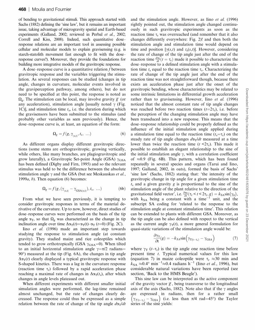
Darwins, the tropic movement involves spatio-temporal

changes in the local stem form. A 3 cm long coleoptile from

a grass seedling, a 50 cm dicot stem or a young 2 m high tree

all share some obvious similarities: active tropic bending is

distributed along the growing zones of the organs and all the

stems tend to curve and de-curve in different places over time

to reach a vertical and mostly straight form at the end of the

movement. The tip of the organ in Fig. 1A and C evenappears to reach a steady vertical orientation whereas the

base is still curving. These spatio-temporal changes in the

distribution of curving and growth make it difficult to

characterize gravitropic movements via any single global

measurement at the whole-organ level. This means that

a significant issue in the study of tropism is how to relate

local changes in angles all along the organ to the global

change in its shape during the movement, to understand therole played by growth and the underlying biological control.

Despite these observations and the early demonstration by

the Darwins that the tip played a much lesser role in shoot

gravitropism than in phototropism (Darwin and Darwin,

1880, confirmed by modern studies, Firn et al., 1981; Tasaka

et al., 1999), tropism research has persisted with a long

tradition of only measuring the inclination angle of the tip

aT. To account for the fact that the tip of the stem might notbe exactly perpendicular to the pot but display an initial

inclination angle aT(0) due to imperfect straightness and

passive mechanical bending under self-weight, some inves-

tigators have defined a ‘curvature angle’ as the change in tip

inclination angle over time, i.e. the difference DaT(t–t0)¼aT(t)

–aT(t¼0) (Hoshino et al., 2007; Tanimoto et al., 2008, to cite

only recent papers). The terminology used is itself quite

varied, ranging from the frequent ‘curvature angle’ or‘bending angle’ to the more confusing ‘curvature (degrees)’

(the reason why it is so confusing will become clear later), but

much more problematically, the spatial positioning of this

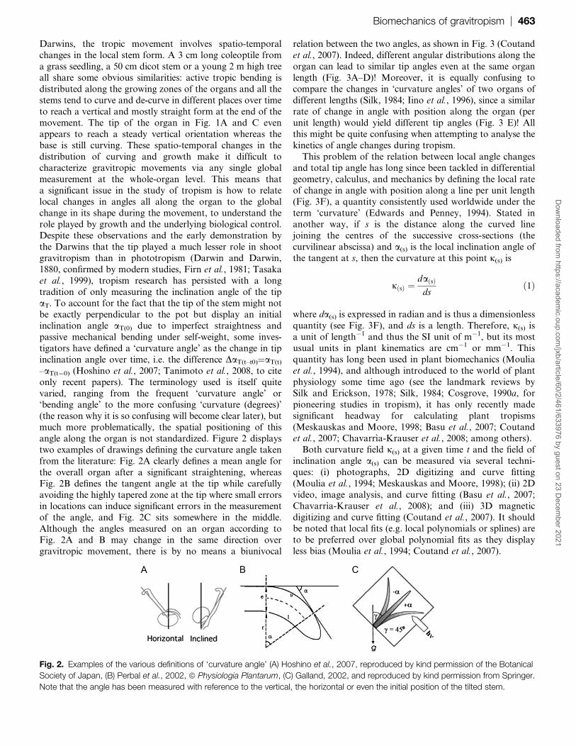
angle along the organ is not standardized. Figure 2 displays

two examples of drawings defining the curvature angle taken

from the literature: Fig. 2A clearly defines a mean angle for

the overall organ after a significant straightening, whereas

Fig. 2B defines the tangent angle at the tip while carefullyavoiding the highly tapered zone at the tip where small errors

in locations can induce significant errors in the measurement

of the angle, and Fig. 2C sits somewhere in the middle.

Although the angles measured on an organ according to

Fig. 2A and B may change in the same direction over

gravitropic movement, there is by no means a biunivocal

relation between the two angles, as shown in Fig. 3 (Coutand

et al., 2007). Indeed, different angular distributions along the

organ can lead to similar tip angles even at the same organ

length (Fig. 3A–D)! Moreover, it is equally confusing to

compare the changes in ‘curvature angles’ of two organs of

different lengths (Silk, 1984; Iino et al., 1996), since a similar

rate of change in angle with position along the organ (per

unit length) would yield different tip angles (Fig. 3 E)! Allthis might be quite confusing when attempting to analyse the

kinetics of angle changes during tropism.

This problem of the relation between local angle changes

and total tip angle has long since been tackled in differential

geometry, calculus, and mechanics by defining the local rate

of change in angle with position along a line per unit length

(Fig. 3F), a quantity consistently used worldwide under the

term ‘curvature’ (Edwards and Penney, 1994). Stated inanother way, if s is the distance along the curved line

joining the centres of the successive cross-sections (the

curvilinear abscissa) and a(s) is the local inclination angle of

the tangent at s, then the curvature at this point j(s) is

jðsÞ ¼daðsÞds

ð1Þ

where da(s) is expressed in radian and is thus a dimensionless

quantity (see Fig. 3F), and ds is a length. Therefore, j(s) is

a unit of length�1 and thus the SI unit of m�1, but its mostusual units in plant kinematics are cm�1 or mm�1. This

quantity has long been used in plant biomechanics (Moulia

et al., 1994), and although introduced to the world of plant

physiology some time ago (see the landmark reviews by

Silk and Erickson, 1978; Silk, 1984; Cosgrove, 1990a, for

pioneering studies in tropism), it has only recently made

significant headway for calculating plant tropisms

(Meskauskas and Moore, 1998; Basu et al., 2007; Coutandet al., 2007; Chavarrıa-Krauser et al., 2008; among others).

Both curvature field j(s) at a given time t and the field of

inclination angle a(s) can be measured via several techni-

ques: (i) photographs, 2D digitizing and curve fitting

(Moulia et al., 1994; Meskauskas and Moore, 1998); (ii) 2D

video, image analysis, and curve fitting (Basu et al., 2007;

Chavarrıa-Krauser et al., 2008); and (iii) 3D magnetic

digitizing and curve fitting (Coutand et al., 2007). It shouldbe noted that local fits (e.g. local polynomials or splines) are

to be preferred over global polynomial fits as they display

less bias (Moulia et al., 1994; Coutand et al., 2007).

Fig. 2. Examples of the various definitions of ‘curvature angle’ (A) Hoshino et al., 2007, reproduced by kind permission of the Botanical

Society of Japan, (B) Perbal et al., 2002, ª Physiologia Plantarum, (C) Galland, 2002, and reproduced by kind permission from Springer.

Note that the angle has been measured with reference to the vertical, the horizontal or even the initial position of the tilted stem.

Biomechanics of gravitropism | 463D

ownloaded from



ber 2021

Curvature has many advantages. It is a local quantity

that can be measured independently of the reference frames.The relationship between angle a(s) and j(s) reflects the fact

that local curving influences the angle of inclination.

Indeed, the increment of angle da(s) between s and s+ds is

da(s)¼j(s)ds, and thus the change in angle Da between the

base s¼0 and the tip s¼L is simply the sum of all the

successive da between the two positions (Fig. 3F), i.e.

Daðbase/tipÞ ¼ aTðs¼LÞ � aBðs¼0Þ

¼ +s¼L

s¼0

daðsÞ ¼Zs¼L

s¼0

daðsÞ ¼ZL

s¼0

jðsÞds ð2Þ

where L is the length of the organ, which can benumerically computed very easily, even with a standardspreadsheet.

Note that equation (2) gives a quantitative explanation ofwhy a longer organ with similar j(s) will display an increased

tip angle whereas the actual bending rate is just the same, as

noted previously (Fig. 3E; Iino et al., 1996). Indeed, solving

equation (2) for a constant curvature j along the axis yields

aTðs¼LÞ ¼ aBðs¼0Þ þ jL (equation 2b), which means that the

tip angle increases proportionally to the length L of the

organ for the same curvature. Numerically, an almost

complete gravitropic movement from an initially horizontal

and straight position can be represented by a final tip angle�aTðs¼LÞ � aBðs¼0Þ

�of 1.5 radians (86�). From equation 2b,

the mean curvature then comes as j¼1.5/L yielding, re-

spectively, curvatures of 0.5 cm�1, 0.1 cm�1, 0.02 cm�1 for

organ lengths of 3 cm, 15 cm, and 75 cm.

Last but not least, working with the assumption that

between-cell adhesion at the middle lamina is maintained [a

validated fact, except for certain extreme cell adhesionmutants, as reported in Krupkova et al. (2007)] and that

there is therefore negligible shear, it is possible to find very

simple relationships between curvature changes, diameter,

and differential elongation or shrinkage of the upper and

lower cell layers. In organs growing only radially through

secondary growth, the computation is direct if, in addition

to curvature field over time j(s,t), the cross-sectional radius

R(s,t) is also known (Coutand et al., 2007). However, tocompute elongating organs requires a deeper specification

of the growth kinematics (Silk and Erickson, 1978; Silk,

1984; Basu et al., 2007; Chavarrıa-Krauser et al., 2008).

Kinematics of growth and differential growth: unravellingthe influences of cell activity and location on curvaturechanges

As the gravitropic response involves growth, a standard

problem in gravitropic studies is to assess how far the effect

on the gravitropic phenotypic performance of say a mutation

or a change in environment can be ascribed (i) to effects on

growth and its spatial distribution along the organ affecting

the gravitropic movement, as opposed to (ii) direct effects on

the gravisensing pathway (Tanimoto et al., 2008).Just as for the rate of curvature, elongation growth is also

distributed spatially, and this distribution is usually non-

homogeneous. As curvature in the primary growing zone

involves local differential elongation growth (Tomos et al.,

1989), it is not sufficient only to measure the total

elongation rate of the organ mT ¼ dLdt

(mT is the tip velocity,

usual unit¼mm h�1, L is the organ length, usual unit¼mm)

or the (mean) relative elongation rate RER ¼ dLLdt

(usualunit¼h�1). The rationale here is exactly the same as

previously used for the comparison between tip angle aT

and curvature field j(s). Cell elongation in organs tends to

stretch the cell irreversibly, so that its length increases over

time. The intensity of this growth-induced stretch at every

position s along the organ can be measured by the

longitudinal strain e(s,t), i.e. by the change in length dl of

a segment of the organ relative to its length l eðs;tÞ ¼ dl=l. Asthis growth-induced stretching is time-dependent, it is

usually better specified by the time-rate of changes in strain,

e_ðs;tÞ ¼@eðs;tÞ@t (d is the partial derivative, here with respect to

time). Thus, the strain rate field specifies at each position

the time-rate of changes in the relative distance between two

successive cross-sections of the growing organ (Fig. 4A).

Some authors prefer to call growth-induced strain rate the

Relative Elemental Growth Rate, REGR (Silk, 1984), but‘strain rate’ is consistent with standard use in mechanics

and is therefore to be preferred.

Fig. 3. Relations between tip angle (ta), local angles (la), and

curvature distribution: (A, B, C, D) different distributions of the local

angle (la) along the organ displaying the same tip angle ta¼aT

(from Coutand et al., 2007, www.plantphys.org, ª American

Society of Plant Biologists), (E) organs with similar rates of changes

in angle with position along the organ sits along a circle, but

different lengths yield different tip angles, (F) definition of the

curvature as the rate of changes in angle with position along the

organ per unit length j¼da/ds: the angle da in radians is equal to

the length of the arc of the tangent circle at point s divided by the

radius of this circle Rj (1 rad is the angle subtended at the centre

of a circle by an arc equal in length to the radius of the circle,

approximately 57�17). The angle da, in radian is thus dimension-

less. The curvature j¼da/ds is the inverse of the radius of

curvature and has units of the inverse of a length (e.g. cm�1).


ownloaded from



ber 2021

www.plantphys.org

As elongating cells stretch, they also push the down-

stream cells next in line, with the result that each cell is

pushed to move by the preceding cells (Fig. 4A). The morecells that are growing upstream, the larger the push, and the

faster the movement velocity (called convection, from the

Latin for ‘moving with’). Elongation growth thus can be

specified using two quantities: (i) the longitudinal velocity

field m(s,t), which defines the growth-induced convective

velocity of any cross-section in an organ at position s and

time t (Fig. 4A), and (ii) the growth-induced strain-rate field

e_ðs;tÞ. Both are related. The difference in velocity betweentwo successive cross-sections separated by the initial dis-

tance ds (Fig. 4A) produces a change in length over time

whose relative time-rate is the longitudinal strain rate, i.e.

e_ðs;tÞ ¼@vðs; tÞ@s

:

Finally, as the growth zone in plant organs is mostly sub-apical, the natural reference frame for the spatial specifica-tion of growth-induced fields is taken at the apex (Fig. 4), sothat s means distance from the apex (curvilinear abscissa).

Elongation growth has major repercussions for theassessment of curvature changes in elongating organs.

Indeed, any given small segment (a group of cells) in the

growth zone will, over time, move away from the tip (Fig.

4B), in a similar way to river flow (Silk, 1984). Because of

this movement, time-derivatives relative to a given position

(distance s measured from the apex) or to a given material

segment (group of cells) do not match anymore. But the

biological mechanisms involved in perception and motor

activity producing curvature changes resides in cells.

Consequently, the biologically relevant rate of change ofcurvature during growth is that of a material segment

(group of cells). This is called the material derivative of the

curvature, which, to distinguish it from the local derivative

in equation (2), is conventionally writtenDjðs;tÞDt

(the upper-

case D distinguishing it from the lowercase d of local

derivative and the @ of the partial derivative). The point

here is that this quantity cannot be estimated simply from

the change in curvature at a given position as in equation(2). For example, if an elongating organ displays a steady

spatial gradient in curvature, then the local change in

curvature is zero (Fig. 4A, B). However, as seen above,

there is a growth-induced convective movement along the

organ, which means the segment is, in fact, producing

a change in curvature, the rate of which depends on (i) how

steep the gradient in local curvature is, i.e. on the rate of

change of the curvature with position at time t@jðs;tÞ@s , and (ii)

how fast it moves with respect to this gradient, i.e. on its

growth-induced convective velocity v(s) (Fig. 4B). In the

most general case, gravitropic primary organs may also

display changes in local curvature at position s (noted@jðs;tÞ@t ),

as illustrated by the change between Fig. 4B and Fig. 4C.

Therefore to compute the ‘real’ rate of change in curvature

of a segment following the growth-push movement, i.e. the

material derivative of curvature, both terms have to besummed and thus the material derivative can be calculated

as (Silk, 1984; Chavarrıa-Krauser, 2006)

Fig. 4. Kinematics of changes in curvature in expanding organs. Three successive states of the same organ are depicted, with their tips

aligned for easier visualization of growth. (A) Initial time t0: transverse marks are set up at distances s0,i (i¼1–5) from the apex, to follow

groups of cells. Dark arrows represents the growth-induced velocity of convective displacement from the apex. Due to differences in

growth-induced velocities, marks closer to the tip convect more slowly than marks further away. This is important for the localization of

groups of cells over time (see B and C). (B) Example of curvature changes mainly due to convection after a time interval dt: although the

spatial distribution of curvature j(s,t) is constant over time, the dark grey segment has moved to a zone of higher curvature by convection

and has thus curved accordingly. (C) Example of curvature changes mainly due local changes: as a rapid local change in curvature has

occurred between (B) and (C) the dark grey segment has changed its curvature while its longitudinal displacement is negligible. Inset:

magnification of the comparison between (A) and (B): the concave side has extended less than the convex side. Comparison between (A)

and (C) shows the superposition of convective (A–B) and local (B–C) changes in curvatures over time.


ownloaded from



ber 2021

Djðs;tÞDt

¼@jðs;tÞ@t

þ vðs;tÞ@jðs;tÞ@s

ð3Þ

-- --- - --- --- ----local convective

Graphically (Fig. 4) equation (3) means that the changes

in the curvature of a material segment of the organ between

Fig. 4A and C (the material derivative) corresponds to the

superimposition of (i) the changes between Fig. 4A and B

(convective changes in the curvature of the segment) and (ii)

the changes between Fig. 4B and C (local changes incurvature). As on-board devices continuously tracking the

material curvature of the organ segments are not available

yet, equation (3) is just a mathematical expression allowing

the material derivative to be computed from the measure-

ment of (i) the local curvature along the organ at various

times (i.e. j(s,t)) and (ii) growth velocity m(s,t) (to be detailed

later). It is also useful to get insights about the positional

versus segment-autonomous controls of curvature changes(Chavarrıa-Krauser, 2006, 2008). Numerically, Silk and

coworkers reported, in hooked lettuce hypocotyls, that

hook maintenance involved convective successive curving

and decurving of stem segments reaching rates up to

2.5 mm�1 h�1 with no local changes (Silk and Erickson,

1978), whereas dramatic changes in the balance between the

two terms were achieved during tropic responses (Silk, 1984).

Finally, in organ parts with no longitudinal elongation andthus negligible growth-induced velocity m(s), as in gravitropic

stems undergoing radial secondary growth (Coutand et al.,

2007) the convective term is always negligible.

The material derivative of curvatureDjðs;tÞDt

characterizes

the tropic bending response of a small segment of a growing

organ. This is the correct quantity to be compared with

cellular changes in the same segment, such as a radial

gradient in auxin content, differences in cytoskeletondynamics or differences in levels of gene expression. It is

also the proper output of a mechanistic model of the

biomechanical motor activity powering the movement (as

will be seen in the third section). In such cases, equations (3)

and (2) will also be required to reconstruct the changes in

stem geometry (length, curvature, and angular distribution,

including tip angle) over time from the material rates of

curvature changes predicted by the biomechanical model.Many studies dealing with differential growth have

focused on the difference in relative elongation rate between

the epidermis on both sides of a curving segment at position

s and time t (Myers et al., 1995; Mullen et al., 1998).

Indeed, as shown in Fig. 4 inset, curving is related to

a higher strain rate in the convex side than in the concave

side, with the mean strain rate of the segment sitting

between the two. The material rate of curvature changesprovides a very straightforward way to compute these

differences in growth-induced strain rate in the segment at

position s at time t. Indeed, if w is the width of the organ in

the (local) plane of bending, so that the epidermis on the

convex side sits at (s,+w/2) and the epidermis of the concave

side sits at (s,–w/2), then the differences in growth-induced

strain rate between the convex and the concave sides can be

readily estimated from the material derivative as:

_eðs;t;þw=2Þ � _eðs;t;�w=2Þ ¼D�jðs;tÞw

�Dt

¼@�jðs;tÞw

�@t

þ mðs;tÞ �@�jðs;tÞw

�@s

ð4Þ

If the width w changes slowly with time and position (low

tapering), as tends to be the case in growing stems and roots

(equation 4), the derivatives of w can be neglected when

applying the Chain Rule in calculating the partial deriva-

tives of the j.w products in equation (4) then yields:

_eðs;t;�w=2Þ � _eðs;t;þw=2Þ �Djðs;tÞDt

� w ð5Þ

Equation (5) states that differential growth is approxi-

mately proportional to the material rate of curvaturechanges multiplied by the organ width, so that wider organs

require more differential growth to achieve the same

material rate of curvature changes and thus the same tropic

movement. For example, an observed material rate of

curvature changes of 0.1 mm�1 h�1on an organ width of 0.5

mm would correspond to a difference in growth-induced

strain rates of 5% h�1, whereas this difference would come to

10% h�1 if the organ width is 1 mm (see Silk, 1984, fora more complete presentation including large strain rates that

should be considered in cases where the product j.w > 0.3).

Direct characterization of growth-induced strain rates in the

epidermis is a possible option (Mullen et al., 1998), but the

results may be less accurate and equation (5) would still be

required in order to relate differential growth to the induced

tropic curvature. Equation (5) conveys the important kinemat-

ical fact that the effect of differential growth on gravitropicbending [and thus on curvature angles through equation (2)]

depends on the width of the organ. It will be shown later that

the dependence on size of the material changes in curvature is

even stronger when taking into consideration the biomechan-

ical motor and the resisting processes involved in producing

the active bending movement (see third section).

Last but not least, the rationale for considering the

material derivative also applies to any content variablealong the organ (Silk, 1984), such as, for example, the

concentration in auxin or any other substance (pH, calcium,

pectins, etc). Indeed, when there is a gradient in concentration

along the organ (a most common feature), then the local rate

of change alone is not enough, as convective changes also

have to be considered such as in equation (3). Since

concentration is based on volume and volume also changes

over time, a dilution term has to be added. This is called thecontinuity equation, and can be found in most papers

analysing growth mechanisms (as summarized in Basu et al.,

2007), and a pedagogical version can be found in Silk (1984).

Several methods based on time-lapse photography or

video could be used to measure the growth-induced strain

rate field e_ðs;tÞ and velocity field m(s,t) and combine them with

the curvature field j(s) to calculate the material derivative of


ownloaded from



ber 2021

curvature (or any material rate of change of substances).

Note that to estimate properly the time-derivatives in equation

(4), the time lapse needs to be small enough to yield a mean

growth-induced strain between two successive frames that is

smaller than 0.2 (Silk, 1984). This condition is not always

fulfilled in published data; overlong time lapses feature not

just in all the original articles (Sachs, 1882) but in some of

the more recent studies as well (Fukaki et al., 1996).The traditional method has been to perform marking experi-

ments as depicted in Fig. 4 and to record their position over

time with time-lapse photography using a appropriate time

lapse (e.g. on stem growth; see Girousse et al., 2005). Genetic

mosaics have been elegantly used to build in marks (Coen

et al., 2004), but their use for kinematics requires a step-by-

step analysis decrementing the past history. Surprisingly,

despite the initial use by Sachs, few gravitropic studies haveused marking experiments with small time lapses (Selker and

Sievers, 1987; Mullen et al., 1998; Miyamoto et al., 2005). In

contrast with the studies on growth responses where kinemat-

ics has became a standard (as rightly pointed out by Basu

et al., 2007), most gravitropism studies persist with the so-

called ‘curvature angle’ to characterize the phenotypic gravi-

tropic response. This might be partly related to the fact that

marking experiments are seen as somewhat tedious and old-fashioned. More recently, bio-imaging techniques have been

developed based on time-lapse photos or videos and automatic

structure–tensor (Schmundt et al., 1998) or image-correlation

analysis (van der Weele et al., 2003; Suppato et al., 2005).

These techniques have been successfully applied to geotropic

roots (Basu et al., 2007; Chavarrıa-Krauser et al., 2008). A

user-friendly freeware is already available, yet too restrictively

named KineRoot as it can actually be used for kinematicalanalysis of any gravitropic response (Basu et al., 2007). These

tools are likely to increase and improve in the near future, and

there is hope that these versatile tools will soon be instrumen-

tal in making kinematical bio-imaging a viable approach for

the majority of teams studying gravitropic responses.

New insights from curvature kinematics: two examples

The kinematic method has been instrumental in characterizing

the Distal Elongation Zone in roots (DEZ) and in defining its

specific function for root-based gravitropic curvature (Mullen

et al., 1998; Chavarrıa-Krauser et al., 2008). This became

possible thanks to the kinematic approach, which is able todistinguish between mean strain rate of the segment, (material)

changes in curvature and differential strain rates with a high

spatio-temporal resolution. More recently, kinematic studies

were able to reveal a clear root phenotype for the pin3-3

mutants in Arabidopsis (Chavarrıa-Krauser et al., 2008). PIN3

is a putative efflux-transporter of auxin and a central candi-

date gene for the control of radial gradient in auxin

concentration, but its function had previously been unclearsince there had been no way decisively to pinpoint the

phenotype of pin3 mutants (Morita and Tasaka, 2004).

Another example is the characterization of a spatio-temporal

pattern of gravitropic curving and autotropic decurving that

seems to be generic to many plants ranging from trees to small

primary organs, despite largely different sizes (Moulia et al.,

2006; Coutand et al., 2007). As shown by the plot of the

spatio-temporal curvature field in Fig. 5, the initial phase of

spatially homogeneous up-curving destabilizes into a counter-

curving spreading downward. This counter-curving occurs

before the tip has overshot the vertical (Fig. 1C). It is therefore

not due to a graviperception of the inclination angle and has

thus been called autotropic ((Firn and Digby, 1979; Tarui andIino, 1997; but see also Stankovic and Volkmann, 1998).

Similar curving dynamics have been reported for wheat and

oat coleoptiles (Fig. 1B) and in the stipe of the Coprinus fungi

(Meskauskas and Moore, 1998; Meskauskas et al., 1999a;

Moulia et al., 2006). However, this very efficient movement,

allowing rapid stabilization of the tip at a vertical position

through autotropic control, is not found in all the plants

(Sierra et al., 2008; Fig. 1A). Autotropism will be discussed inmore detail in the modelling and ecology sections.

These two examples demonstrate that a spatio-temporal

kinematics approach, based on the distribution of the

material time-derivative of the curvature and the distribu-

tion of growth-induced strain rates and velocities, has led to

a deeper understanding of the mechanisms involved in

gravitropism, increased the capabilities of phenotyping

mutants, and opened the search for common patterns ofregulation in different organs and/or species.

Dose–response curves for angularperception, gravitropic sensitivity andcontrol

Macroscopic phenomenology: the sine rule

Once the movement has been properly quantified, the next step

may be to establish a dose–response curve relating the kinematics

Fig. 5. Spatio-temporal field of curvature during the gravitropic-

autotropic straightening movement of poplar stems (Coutand et al.,

2007, www.plantphys.org, ª American Society of Plant Biologists).


ownloaded from



ber 2021

www.plantphys.org

of bending to gravitational stimuli. This approach started with

Sachs (1882) defining the ‘sine law’, but it remains an important

issue, taking advantage of microgravity spatial and Earth-based

experiments (Galland, 2002; reviewed in Perbal et al., 2002;

Correll and Kiss, 2008). Indeed, such quantitative dose–

response relations are an important tool in assessing possible

cellular and molecular models to explain gravisensing (e.g. is

starch-statolith movement fast enough to fit with the dose–response curves?). Moreover, they provide the foundations for

building more integrative models of the gravitropic response.

A dose–response curve is a quantitative relation f between

gravitropic response and the variables triggering the stimu-

lation. As several responses can be studied (changes in tip

angle, changes in curvature, molecular events involved in

the graviperception pathway, among others), but do not

need to be specified at this point, the response is noted asXg. The stimulation can be local, may involve gravity g/ (or

any acceleration), stimulation angle [usually noted c (Fig.

1C)], and stimulation time ts, i.e. the duration during which

the gravisensors have been submitted to the stimulus (and

probably other variables as seen previously). Hence, the

dose–response curve is, at least, an equation of the form:

Xg ¼ f ðg; cðs;tÞ; ts; .Þ ð6Þ

As different organs display different gravitropic direc-

tions (some stems are orthogravitropic, growing vertically,

while others, like many branches, are plagiogravitropic and

grow laterally), a Gravitropic Set-point Angle (GSA) cGSA

has been defined (Digby and Firn, 1995) and so the relevantstimulus was held to be the difference between the absolute

stimulation angle c and the GSA (but see Meskauskas et al.,

1999a, b). Then equation (6) becomes:

Xg ¼ f ðg; ðcðs;tÞ � cGSAðs;tÞÞ; ts; .Þ ð6bÞ

From what we have seen previously, it is tempting toconsider gravitropic responses in terms of the material de-

rivative of the curvature. Up to now, however, direct studies of

dose–response curves were performed on the basis of the tip

angle aT, so that Xg was characterized as the change in tip

inclination angle over time DaT(t)¼aT(t)–aT (t¼0) (Fig. 2C).

Iino et al. (1996) made an important step towards

studying the response to stimulation angle (at constant

gravity). They studied maize and rice coleoptiles whichtended to grow orthotropically (GSA cGSA¼0). When tilted

to an initial horizontal stimulation angle c¼p/2 radians¼90�) measured at the tip (Fig. 6A), the changes in tip angle

DaT(t) clearly displayed a typical gravitropic response with

S-shaped kinetics. There was a lag in the curvature response

(reaction time sr) followed by a rapid acceleration phase

reaching a maximal rate of changes in DaT(ts), after which

changes in angle levels plateaued out.When different experiments with different smaller initial

simulation angles were performed, the lag-time remained

almost unchanged, but the rate of changes clearly de-

creased. The response could thus be expressed as a simple

relation between the rate of change of the tip angle daT/dt

and the stimulation angle. However, as Iino et al. (1996)

rightly pointed out, the stimulation angle changed continu-

ously in such gravitropic experiments as soon as the

reaction time sr was overreached (and remember that it also

changes differently everywhere: Fig. 2)! and then both the

stimulation angle and stimulation time would depend on

time and position [c(s,t) and ts(s,t)]. However, considering

the rate of change of the tip angle just after the end of thereaction time daT

dtðt ¼ srÞ made it possible to characterize the

dose–response to a defined stimulation angle with a stimula-

tion time ts equal to the reaction time sr. Characterizing the

rate of change of the tip angle just after the end of the

reaction time was not straightforward though, because there

exists an acceleration phase just after the onset of the

gravitropic bending, whose characteristics may be related to

some intrinsic limitations in differential growth accelerationrather than to gravisensing. However, Iino et al. (1996)

noticed that the almost constant rate of tip angle changes

was reached before two reaction times (t¼2sr), i.e. before

the perception of the changing stimulation angle may have

been transduced into a new response. This means that the

dose–response relationship could be properly defined as the

influence of the initial stimulation angle applied during

a stimulation time equal to the reaction time (ts¼sr) on thesteady rate of tip angle changes daT/dt measured at a time

lower than twice the reaction time (t <2sr). This made it

possible to establish an elegant relationship to the sine of

the initial stimulation angle c, with a correlation coefficient

of �0.9 (Fig. 6B). This pattern, which has been found

repeatedly in several species and organs (Tarui and Iino,

1997; Galland, 2002, in oats), formed the basis of Sachs’

‘sine law’ (Sachs, 1882) stating that: ‘the intensity of thegravitropic change in tip angle for a given stimulation time

ts and a given gravity g is proportional to the sine of the

stimulation angle of the plant relative to the direction of the

gravitational field vector’, i.e. @aT@t ðsr < t< 2sr; gÞ ¼ kSAsin

�c0

�,

with kSA being a constant with a time�1 unit, and the

subscript SA coding for ‘related to the response to the

stimulation angle at constant stimulation time’. This relation

can be extended to plants with different GSA. Moreover, asthe tip angle can be also defined with respect to the vertical

as the current angle cT(t), a more general formulation for

quasi-static variations of the stimulation angle would be:

@cT@t

ðgÞ ¼ �kSAsin�cTðt�srÞ � cGSA

�ð7Þ

where cT (t–sr) is the tip angle one reaction time beforepresent time t. Typical numerical values for this law(equation 7) in maize coleoptile were sr �30 min andkSA �0.4� min�1�0.4 radians h�1 (Iino et al., 1996), butconsiderable natural variations have been reported (seesection, ‘Back to the HMS Beagle’).

This sine law can be interpreted as the active component

of the gravity vector g/, being transverse to the longitudinal

axis of the axis (Sachs, 1882). Note also that if the c angles

are expressed in radians, then for a rather small�cTðt�srÞ � cGSA

�(i.e. less than p/4 rad¼45�) the Taylor

series of the sine yields:


ownloaded from



ber 2021

@cT@t

ðgÞ � �kSA

�cTðt�srÞ � cGSA

�ð7bÞ

with less than 10% approximation.Defining the dose–reponse as in equation 6B requires the

additional analysis of the effects of the stimulation time tsand of the gravity-induced acceleration g. In tilting experi-ments run on Earth, as in Iino et al. (1996), it is, however,

impossible to control stimulation time ts (as we have seen

that this is determined by the reaction time sr of the plant),

nor the gravity-induced acceleration g. To do so takes two

other types of experiments (i) rotating the plants slowly

around their axis in a 2D clinostat or randomly in a 3D

clinostat, making the gravitational stimulus isotropic (see

Larsen, 1969, and Pickard, 1973, for ingenious experiments

using a 2D clinostat), or (ii) using a centrifuge and/or

microgravity to model the acceleration and mimic the range

from hypergravity to microgravity (reviewed in Correll and

Kiss, 2008). These options all have their limits, in particular,the fact that fast mechanical deformations (bending during

clinostatic rotation, vibrations, etc) might activate mechano-

sensors that may affect both growth (thigmomorphogenesis;

Coutand and Moulia, 2000) and the gravisensitivity itself

(LaMotte and Pickard, 2004; Telewski, 2006). These studies

mostly confirmed that the sine law gives a good fit for small

stimulation times ts close to the minimal time that yielded

a noticeable bending response (called the presentation timesp; Larsen, 1969); or at least for stimulation times that are

small enough ahead of the reaction time (ts/sr <10�1).

Considering larger stimulation times or different acceler-

ation fields yielded more complex dose–response curves.

The relation between the response and ts (or the gravistimu-

latory dose Sd¼g3ts) exhibits a log or, more probably,

a hyperbolic shape (Perbal et al., 2002), the latter suggesting

that even very small doses (or presentation times) may besensed and that saturation is to be expected with large

stimulations. Moreover, increasing the presentation time

yielded an increasingly skewed curve for the response to the

stimulation angle cT. This curve displayed maximal

responses at angles close to 2p/3 rad (120�), thus departing

from a sine distribution, especially for angles higher than

p/2 rad (90�) (Larsen, 1969; Galland, 2002). Several models

have introduced an inhibitory multiplicative (1–cos(cT))term related to the effect of the axial component of gravity

(see Audus, 1964, for a review).

Even at small ts and constant g3ts, Iino et al. (1996)

reported a clear saturation for the response to rice

coleoptiles (Fig. 6C), showing that the range of validity of

the sine law may be species-dependent. Finally, when

graviresponses occur with light (Galland, 2002), which is

a feature relevant to shoot gravitropism in natural con-ditions, there was a phototropism-mediated change in GSA

(with exponential dependency on fluence rate), yielding

photo-gravitropic equilibrium (Galland, 2002: see Iino,

2006, for a more detailed review and discussion).

These more complex effects, in particular, the sine and

cosine terms, have been interpreted as revealing underlying

competing mechanisms in the cellular–molecular process of

graviperception. However, as shown before, the tip-angleresponse considered in all these studies is an integration of

all the local bending responses along the organ [see

equation (2)]. Moreover, in stems and coleoptiles the

gravisensing competency is distributed in the endodermis

that spans the entire stem length (Tasaka et al., 1999;

Morita and Tasaka, 2004). The previous dose–responses are

thus really big black boxes! Lastly, as soon as stimulation

time ts creeps beyond reaction time sr, the stimulation anglec(s,t) changes continuously (and this will affect the response

from as early as ts >2sr).

Fig. 6. Dose–response curves for the rate in change in tip angle

versus initial stimulation angle c (from Iino et al., 1996, reproduced

by kind permission of Blackwell Publishing). (A) Kinetics of

changes in tip angle at different initial stimulation angle c for maize

coleoptiles; (B, C) relation between the rate of change in tip angle

and the sine of the stimulation angle in maize (B) and rice (C).


ownloaded from



ber 2021

It would be much more informative to establish dose–

response curves directly incorporating the material rate of

curvature changesDjðs;tÞDt

and equations (4) and (5), but to the

best of our knowledge, this has not yet been done in shoot

organs [the situation is a bit different in roots as there is

consensus that gravisensing is restricted to the tip: see

Chavarrıa-Krauser et al. (2008) for a detailed kinematical

analysis in root systems, but see also Wolverton et al. (2002)showing that the gravisensing may be more distributed in

roots also]. Measurements of differential strain between the

concave and the convex sides of the organ at the scale of

a small element are the most closely responses that have been

studied so far [see equation (5)]. Myers et al. (1995) did report

such measurements at several initial stimulation angles and

argued that they may not fit a sine law, but no dose–response

characterizations have been produced. Insights from thecellular mechanisms determining graviperception and the

bending response and their spatio-temporal distribution over

the course of gravitropic stimulation and the gravitropic

response may well prove informative on this point.

A brief overview of the molecular and cellular biology ofgravisensing

The topic has been covered in detail in recent reviews (Kiss,

2000; Blancaflor and Masson, 2003; Haswell, 2003; Perbal

and Driss-Ecole, 2003; Morita and Tasaka, 2004; Iino,

2006; Gilroy and Masson, 2008), and thus only the major

features relevant from a biomechanical point of view will besummarized here, essentially for non-specialist readers.

These features mainly involve two longstanding (though

evolving) qualitative models: the ‘starch-statolith’ theory

and the ‘Cholodny–Went’ theory.

The perception of gravity in aerial organs is localized in

a specific tissue, the endodermis in dicot young stems and

inflorescences and the starch-sheath in monocot pulvini

(Morita and Tasaka, 2004) and woody stems (Nakamuraet al., 2001). These tissues have specialized cells called

statocytes, usually containing large starch-filled plastids or

amyloplasts. Mutants lacking proper endodermis differenti-

ation are agravitropic (Tasaka et al., 1999; Morita and

Tasaka, 2004). Moreover, most of the perception of the

dose and orientation of the gravitational stimulus in these

cells is related to the downward movement of the amylo-

plasts, which thus function as statoliths. This downwardmovement would allow them to activate trans-membrane

receptors, possibly mechanosensitive channels triggering

Ca2+ influxes and InsP3 amplification (Perbal and Driss

Ecole, 2003; Valster and Blancaflor, 2008), and eventually

switching on gene transduction.

Indeed, amyloplast mutants lacking starch or with re-

duced starch content display reduced gravitropic response,

whereas mutants with excess starch display an enhancedresponse (Tanimoto et al., 2008). By the same token, shoots

with reduced starch content due to carbon starvation (i.e.

dark or a deep shade) are also less responsive. Moreover,

using a high-gradient magnetic field (HGMF) exerting

a ponderomotive force on endogenous amyloplasts, Weise

et al. (2000) were able to demonstrate that tropic curvature

is induced locally in stems, i.e. only occurring in regions

growing and displaying amyloplast displacement. HGMF-

induced amyloplast displacement in the lignified basal part

of the stem, for example, had no effect on tropic curvature.

The perception of orientation versus gravity and of the

corresponding dose of gravistimulation thus involves amy-

loplast movements in the direction of gravity, in accordancewith the longstanding ‘Starch-statolith’ theory. Note, how-

ever, that mutants lacking downward amyloplast movements

still display a weak gravitropic response, which suggests that

amyloplast statoliths seem to be an evolutionary mechanism

for amplifying gravisensitivity, in addition to a presumably

ancient mechanism related to the direct sensing of protoplast

pressure (Perbal and Driss Ecole, 2003).

The movement of the starch-filled statoliths does prove tobe more complex than initially thought. The high density of

starch compared to mean cytoplasmic content means their

weight overcomes the buoyancy reaction and the viscoelas-

tic friction of the cytoplasm, with the result that sedimenta-

tion can occur. However, amyloplast movement is clearly

regulated by interactions with vacuoles and vacuole traf-

ficking, especially in shoot statocytes (Morita and Tasaka,

2004; Saito et al., 2005). Moreover, reports have citeda direct influence of the actin cytoskeleton and also of

actin–myosin molecular motors (Palmieri et al., 2007).

Interestingly, it has been argued that the actin cytoskeleton

may down-regulate gravitropism by continuously resetting

the graviperceptive system and by controlling the signal-to-

noise ratio (Morita and Taska, 2004; Palmieri et al., 2007).

This raises the important issue of putative accommodation

of the sensitivity of the gravisensing system (LaMotte andPickard, 2001; Moulia et al., 2006). Indeed, it has been

shown in roots that statocytes grown in microgravity are

more sensitive than those grown on a 1 g centrifuge in space

(Perbal and Driss-Ecole, 2003). This is consistent with older

reports that clinostatted plants subsequently show increased

graviresponses (Audus, 1969). This accommodation of

gravisensitivity might be partially reflected by the logarith-

mic dependence of the macroscopic gravitropic response Xg

on the stimulation dose Sd: Xg¼k(c)+llog(Sd). Indeed, the

increment of response @Xg due to an increment in the

stimulation dose @Sd then becomes:

@Xg ¼lSd

@Sd ð8Þ

so that sensitivity to a variation in the dose of thestimulus is inversely proportional to the current level ofthe stimulus, meaning very fast accommodation.

However, the model in equation (8) is likely to be

insufficient (Perbal et al., 2002) and the specific process of

accommodation with its specific time scales will have to be

given more in-depth analysis. By the same token, themolecular mechanisms underlying the modulation of the

Gravity Setpoint Angle by development or environmental

cues remain unknown.

More insights into the dynamics of amyloplast move-

ments might come from the recent techniques of in vivo


ownloaded from



ber 2021

imaging. In particular, the confocal imaging of the Pt-GFP

transgenic line of Arabidopsis with its Green Fluorescent

Protein expressed exclusively in the amyloplast of the

endodermis (Palmieri et al., 2007) should be particularly

informative. It might also stimulate the new generation of

formalized bio-physical modelling that is necessary to

further our understanding of the dynamics of the gravisens-

ing cell and to build systems biology models of gravipercep-tion (since the active modelling activity of the pioneers,

including the elegant work by Audus, 1964, has unfortu-

nately faded away). There is currently no cellular-based

mechanistic model that could replace/improve phenomeno-

logical sine law for quantitative studies and integrative

organ modelling.

The downward movement of amyloplasts, as sensed

through mechanoreception, is thought to interact with thePIN3 auxin efflux transporter, which is located exclusively

in the inner side of the endodermis and facilitates centripe-

tal auxin efflux. This is likely to establish a link with the

other major feature of the current view on gravitropism: the

asymmetric radial polar transport of the plant hormone

auxin (see Tanaka et al., 2006, and Muday and Rahman,

2008, for recent reviews). Auxin moves along the stem to

the root through a unique polarized transport mechanisminvolving several cellular influx and efflux transporters and,

in particular, the specific localization of efflux transporters

from the PIN and probably MDRP/PGP families.

This polar transport of auxin results in axial auxin

gradients down the stem, peaking in the stem growth zone

(Muday and Rahman, 2008). Upon gravistimulation, by

reorientation and relocalization/activation of PIN3 auxin

transporters (and/or other auxin transporters), a transverse(radial) gradient builds up across the stem, with peak auxin

concentration in the lower side. This difference in concen-

tration is supposed to drive the motors of the gavitropic

response differentially. The literature now refers to this

qualitative model as the ‘Cholodny–Went hypothesis’ (see,

however, Firn and Digby, 1980, for a more informative

historical view). Although the debate continues (Firn et al.,

1981), this hypothesis has received considerable supportfrom radio-labelling, molecular and genetic studies (see

Tanaka et al., 2006; Du and Yamamoto, 2007; Muday and

Rahman, 2008, for more detailed arguments). Philippar

et al. (1999) used ultra-precise gas chromatography-mass

spectroscopy (GC-MS) directly to quantify auxin concen-

trations in maize coleoptiles with high resolution. Upon

gravistimulation, two changes in auxin gradients were

observed (Fig. 7): (i) a rise in the longitudinal gradient withincreased free auxin near the tip within 5–10 min, and (ii)

after 15 min, the onset of a ‘Cholodny–Went-like’ up–down

gradient, starting from the tip and proceeding down the

coleoptile within 45 min. Unfortunately, there was no

attempt to model these results mathematically. Moreover,

this view may still be too simplistic. Indeed, the control of

polarized auxin transport is much more dynamic than the

classical description outlined above. It involves complextransporter endosome trafficking (again involving molecular

actin–myosin motors) and feedbacks from auxin itself (plus

other regulators, including ethylene and InsP3, both of

which are also associated with mechanotransduction, and

others such as flavonoids). Moreover, the regulation of

auxin sensitivity seems to be required for asymmetric gene

expression (Salisbury and Ross, 1992) and auxin-dependent

and auxin-independent pathways may co-exist (Yoshihara

and Iino, 2007). Last but not least, some responses cannot

be fully explained through the current ‘Cholodny–Went’theory. For example, the dampened oscillations alternating

bending and counter-bending that occur before reaching

a stabilized vertical GSA position (Fig. 5) are not matched

by preceding oscillations in auxin transport and across-

organ concentration (Haga and Iino, 2006), although

a steady asymmetric auxin gradient is required (Dolk,

1936). Bioassays, radiolabelling, and GC-MS analyses in

tree stem with secondary growth and reaction wood-mediated gravitropism have yielded contradictory results as

to the possible transverse gradients in auxin concentration,

although the dominant, yet debated, view is that transverse

gradients of auxin are involved in i) compression wood

formation, in interactions with ethylene, and ii) possibly

also in tension wood, in interaction with gibberellins.

Nevertheless, a direct influence of bending perception per se

(besides that of auxin gradients) is also involved (Du andYamamoto, 2007).

Most of the recent reviews on gravitropism usually stop

here. Some add a short paragraph on the action of auxin on

cellular expansion, usually detailing some of the many

downstream regulated genes. However, at this point,

nothing has yet been said about ‘the power of movement’!

Indeed, power in science has a clear meaning: the time-rate

of delivering free energy, by doing work for example (it islikely that this thermodynamics-based meaning of power

Fig. 7. Redistribution of endogenous auxin (indole acetic acid,

IAA) concentrations during the early phase of the gravitropic

movement of coleoptiles in response to a 90� gravi-stimulation

(see also Fig. 1B). (A) Gravitropic movement between 0 min and

60 min; (B) IAA concentration (pg IAA mg�1 fresh weight) in

0.5 cm segments of coleoptile halves decomposed into seven

concentration ranges and colour-coded; (C, D) endogenous IAA

concentrations in coleoptiles gravi-stimulated for 0, 5, 10, 15, 30, 45,

and 60 min (from Philippar et al., 1999, ª National Academy of

Sciences, USA).


ownloaded from



ber 2021

was prevalent in the Darwins’ mind when they wrote their

book, as Joule and Helmholtz’s works dates back to the

1840s, but we leave this point to the historians of Science).

Power has its SI unit Joules per second (or Watts), and is

also expressible as the product of the force applied to move

an object and the velocity of the object in the direction of

the force (Power, 2008). The power of movements would

thus measure a flux of free energy that is necessary to bendthe organ and to move it back to its GSA. Understanding

the power of movement thus requires a response to

questions of the motors involved and the resistances to this

active movement. Furthermore, as gravitropic bending is a

whole-organ response, the cellular level is not enough. How

are organ anatomy and morphology related to the rate of

curvature change Dj(s,t)/Dt and to the changes in tip angle?

The power of tropic movement: motors andresistances

A motor is a device that transforms some potential free

energy into work (at a time-rate characterizing its power).

At the cellular level, plants have two major motors (Moulia

et al., 2006). The first one is an osmo-hydraulic motor

(OsmH motor; Fig. 8A1) and is found in cells with primary

cell walls. The second is a polymeric swelling/shrinkage

motor (PSS motor; Fig. 8B1), and is found in cells with

secondary cell walls.A resistance is a biophysical process that counteracts the

motor system by absorbing part of the free energy, either by

storing it in a potential form that cannot be used for

producing the movement (e.g. blocking of the gravitropic

movement by a stiff stake storing elastic energy out of the

gravitropic organ; Yamashita et al., 2007; Ikushima et al.,

2008) or by dissipating this free energy into heat (a

degraded form of energy) through some friction. There aretwo types of resistances: those internal to the motor

(reducing its energetic efficiency) and those external.

Osmo-hydraulic motors

Osmo-hydraulic motors can be found in apical growth

zones of stems and roots, and in intercalary primary growth

zones such as grass pulvini or grass blade joints (Moulia

et al., 2006). Their major features are summarized in

another long-standing model, that of Lockhart (Lockhart,1965; see review in Tomos et al., 1989; Ortega, 1994; and see

Dumais et al., 2006, for the most recent update, although

applied to the case of tip growth). Lockhart’s model was set

up in the 1960s after several decades of physiological

research starting with Pfeffer’s work in 1877 (discussed by

the Darwins in ‘The power of movement’, see also Pfeffer,

2008, in Encyclopaedia Britannica); but the advance brought

by Lockhart was to turn a qualitative hypothesis intoa quantitative biophysical structure–function model. As

plant cells are surrounded by a stiff cell wall and the

deposition of cell wall polymers occurs at the interface

between the inner face of the cell wall and the plasma

membrane (Johansen et al., 2006), the irreversible changes

in length during growth require a cell wall able to stretch

irreversibly over time, i.e. displaying creep (Fig. 8A1). This

creep can be measured by the time-rate of change of its

relative length, i.e. the growth-induced longitudinal strain

rate e_ðs;tÞ (as defined in the section about kinematics). It has

been experimentally demonstrated that the work required

for this irreversible stretching involves longitudinal stresses

in the cell-wall r. These stresses represent internal forces perunit surface area (units MPa) acting longitudinally within

the cell wall (there are in fact stresses acting in all three

directions, but only the longitudinal component works

towards elongation here). They arise from the reaction of

the cell wall to the turgor pressure P of the cell, as well as to

any external loads rext from neighbouring cells or from the

environment (external loads are expressed as the resulting

force per unit cross-sectional area of the tissue rext to keepthem harmonized with turgor pressure P). Creep only

occurs after a minimal stress or (plastic) yield threshold ry

has been reached, and permanent work is required to

maintain a given strain rate e_ðs;tÞ due to the viscoplastic

resistance of the cell wall itself, which dissipates part of the

work into heat. Moreover, elastic cell stretching may occur

in response to changes in turgor pressure or external load.

By setting a biomechanical model based on minimalparameterization of this anisotropic visco-elasto-plastic cell

wall behaviour, and resolving the mechanical equilibrium

for a cylindrical cell with longitudinal extension only

(anisotropic growth), the previous description of the

experimental results can be summarized into the following

equation (Ortega, 1994):

_eðtÞ ¼1

U�1ðtÞ

�PðtÞ þ rextðtÞ � PYðtÞ

�þ 1

Eð _PðtÞ þ r_ extðtÞÞ ð9Þ

-- -- - ---- ---- ---- ---- --- -- ---- ---- ---- ---

Strain rate viscoplastic¼growth elastic¼ reversible

where e_ ðs;tÞ is the longitudinal strain rate, P is the turgorpressure, rext is the external longitudinal stress, P_ andr_ ext are time-rate of change in P and rext, PY, U, and Eare global cell mechanical properties (see details below).Note that the P and r variables must be expressed in thesame unit (for example, MPa).

This equation means that power from turgor pressure P

and, eventually, neighbouring cells rext is required for the

cell wall extension to overcome two types of internal

resistances: visco-plastic extension of the cell wall, and the

housing of potential elastic energy into the cell wall.The visco-plastic creep is the irreversible growth compo-

nent found in growing cells; it is characterized by two

parameters PY and U. PY is the pressure (and/or any external

forces per unit surface over the entire cell) required to reach

the plastic yield point of the cell, U is the visco-plastic

extensibility of the cell in relation to the rheological processes

in the cell wall (internal frictions and bound ruptures) and to

the relative thickness of the cell wall versus cell radius; U�1,its inverse, is the visco-plastic resistance of the cell.

The elastic extension is a reversible term (i.e. it can be recovered

upon de-loading, such as through plasmolysis, provided there


ownloaded from



ber 2021

have not been too many cell wall deposition; Peters and Tomos,

2000). It can be found in all the cells, and is characterized in

this simple model by one parameter, E, which is the bulk elastic

stiffness of the cell wall in relation to the mean elastic stiffness

of the cell wall material (its Young’s modulus) and to therelative thickness of the cell wall versus cell radius.

In cells undergoing steady growth conditions ( _P and r_ ext � 0)

with no external load (rext �0), cells may grow typically at

e_ ðs;tÞ¼1% h�1 in stems (Girousse et al., 2005). In tissues

undergoing steady growth, P is typically �0.5 MPa (Tomos

et al., 1989). Assuming a yield threshold of around 0.25 MPa,

the visco-plastic resistance of the cell wall U�1comes to 25 MPa

h, meaning that 25 MPa above the yield threshold, i.e. 250 bars(!), would be required to double the size of the cell every hour,

working against cell wall resistance (this is probably exceeding

the wall strength though).

In natural (non-steady) conditions, all the parameters in

equation (9) may change with time and thus have a (t) index.

These changes are usually under biological control. However,

the only biological controls that are relevant for gravitropism

are those differentially expressed between the concave and

convex sides during gravitropic movement (Fig. 8A2; Tomos

et al., 1989; Cosgrove, 1990b). The visco-plastic resistance ofthe cell wall decreases quickly with auxin, at least in the

epidermal outer cell wall (see Kutschera and Niklas, 2007 for

a review). This is probably due to cell wall acidification

triggering expansin-dependent weakening of hydrogen bonds

and, in the longer term, to auxin-induced expression of

expansin (Muday and Rahman, 2008, but see counter-

arguments in Ikushima et al., 2008). Differential changes in

pectin and xyloglucan polymer size in the upper and lowerparts of bean epicotyls also correlates to differential changes

in wall extensibility as a response to inclination, and not

bending (Ikushima et al,. 2008). Such changes may also be

triggered by auxin through the induction of xyloglucan endo-

transglucosylase/hydrolase (XTH), and/or changes in

Fig. 8. The two basic types of motors producing mechanical work, deformation and movements in plants, at cell level (left) and at organ

segment level (right). (A) Hydraulic motors in primary (non-woody) tissues: (A1) diagram of a cell showing the reversible or irreversible

stretching of the cell wall under hydrostatic (turgor) pressure due to internal osmotic potential and possible external stresses. The cross-

arrow inside the cell sketches out internal hydrostatic pressure. This hydrostatic pressure and the external stresses are balanced by

internal stresses (arrows) in the cell wall that result from the mechanical stiffness of the cell wall under stretching. A water flux enters the

cell (left arrow) due to differences in water potential between the inside and the outside of the cell. This difference provides the free

energy for the work of cell-wall stretching. If elastic stretching occurs, then this energy is stored as potential elastic energy in the cell wall.

If irreversible stretching (growth) occurs, then part of this energy is dissipated by the cell wall viscosity (A2); if the hydraulic stretching of

cells is heterogeneous across the cross-section of the stem, active bending occurs. (B) Cumulative shrinkage/swelling motors in

secondary woody tissues (illustrated here in angiosperms): (B1) diagram showing the motor effects of the addition of an outer cell layer

(4) produced by secondary growth (dashed arrow) to older layers (1 to 3) and the cell-wall differentiation (maturation) of this outer layer

(4). With polymerization in the secondary cell wall, the maturing new cell layer tends to shrink longitudinally (drawing at top). However, this

maturation shrinkage is not possible, as it is limited by older layers (drawing at bottom). The new cell layer is thus put into a state of

tension (external arrows), whereas the inner layers (that were initially in tension due to their own maturation shrinkage) experience an

increment in compression (internal arrows). As the process is reiterated with new layers, successive compressions accumulate (additional

arrows indicate accumulating compression stresses). (B2) If this shrinkage is heterogeneous across the cross-section of the stem (such as

when tension wood is produced), then active stem bending occurs. (Adapted from Moulia et al., 2006, and reproduced by kind permission

of the Botanical Society of America.) (TW, tension wood; NW, normal wood.)


ownloaded from



ber 2021

exocytotic rate of matrix polymer deposition (see Ikushima

et al., 2008, for a review). Note that it is bending, but not

inclination angle, that has been shown to induce differential

changes in the cortical microtubules (MT) between the upper

and lower epidermis during gravitropic movement. MT

orientation is usually related to the orientation of the

‘extrusion’ of cellulose microfibrils in the cell wall and thus

to cell-wall extensibility (Ikushima and Shimmen, 2005),providing evidence for the involvement of a mechanopercep-

tive control over bending rate in gravitropism (independently

of auxin and of inclination sensing).

As highlighted by the Darwins (1880), differential pressure

in the upper and lower part is also a candidate explanation

for differential growth during tropisms. However, direct

measurements using cellular pressure probes demonstrate

that, although changes in pressure do induce changes instrain rate in plants, no significant difference in pressure has

been observed between the upper and lower parts of

graviresponding organs (Tomos et al., 1989; Cosgrove,

1990b, Kutschera and Niklas, 2007; Ikushima et al., 2008).

However, cell wall yielding under pressure is not sufficient to

understand cell growth fully. The increased cell volume is filled

with water (so no vacuum can occur), meaning that water

influx needs to be coupled with pressure-driven expansion (Fig.8A1). This is likely to occur through passive water flow. The

power for this influx is related to the gradient in the water

potential W between the interior of the cell and the water

source (the water potential is the amount of work that would

be necessary to bring a unit volume of water back into

a reference state of free water at atmospheric pressure and

constant temperature; W is by convention a negative, and its

unit of expression is MPa). This kind of gradient existsbecause an osmotic potential, –Pi, is maintained within the

cell. The resistance Rh to this water flow is due to water

pathway-long ‘frictions’. This includes the hydraulic resistance

not only of the cell membrane but also throughout the path of

water flow from the source to the growing cell (Tomos et al.,

1989). This can be stated in the second Lockhart equation:

e_ðtÞ ¼1

RhðtÞ��PextðtÞ � PðtÞ

�� r

�PextðtÞ �PiðtÞ

��ð10Þ

where Pext is the pressure of the external water source, P isthe internal turgor pressure, r is the reflection coefficient ofthe membrane (a parameter ranging from 0 to 1 and mea-suring the degree of hemipermeability, 1¼permeable onlyto water), –Pext is its osmotic potential (i.e. Pext is itsosmotic pressure), and (Pext–Pext) is the water potentialWext of the external source, Rh is the integrated resistance towater flow. Equation (10) says that the growth-inducedstrain rate depends on the differences between hydrostaticand osmotic pressures in the external source and inside thecell. The water pathway and thus its integrated resistanceRh can vary significantly within the same organ dependingon whether it grows in air or in water (e.g. submergedversus air-grown rice coleoptiles, see Fig. 3, or aeroponicroots versus hydroponic roots). But resistance along thewater pathway is not the only source of resistance to waterinflux. A lower Wext (i.e. small Pext and/or large osmotic

content Pext) results in less water available for growth (as isthe case during water stresses). In addition, equation (10)shows that a high turgor pressure P tends to squeeze waterout of the cell. Thus turgor pressure has an opposite effectin equations (9) and (10).

Actually, equation (10) is insufficient. Water influx is only

possible if the internal water potential is actively andbiologically maintained by adjustments of the internal osmotic

potential –Pi of the cell and by the maintenance of the cell’s

(almost) hemipermeable membranes (both involving consump-

tion of metabolic energy). Although rarely cited in reviews,

this leads to a third equation expressing the changes in

internal osmotic potential –PI (assuming the Van’t Hoff

equation for osmotic pressure in diluted solutions, and

neglecting Onsager’s coupling between passive water and ionicfluxes , i.e. r¼1; see Boyer and Silk, 2004):

dPiðtÞPiðtÞdt

¼ 1

n

�dn

dt

�� 1

V

�dV

dt

�¼ 1

n

�dn

dt

�� _e ð11Þ

-- ---- --- - --- ---- ---- --- -

Osmotic

adjustmentDilution bywater flux

Growth-inducedstrain rate

where n is the number of osmoles in the cell vacuole andV is the cell volume.

Equation (11) just states that osmotic adjustment by

changing the number of osmoles n has to match the dilution

by water influx due to the growth-induced strain rate in

order for the osmotic pressure to be maintained and for the

osmohydraulic motor to maintain steady work. This

adjustment is thought to involve strain or strain-rate

mechanosensing by mechanosensitive channels (Telewski,2006), which makes sense from equation (11). It may

involve membrane transporters actively pumping (i) ions

(e.g. potassium K+) from the surrounding apoplast, (ii)

amino acids arriving from phloem downloading (e.g. pro-

line), as well as the hydrolysis of polymers into monomers,

for example, starch from amyloplasts (Tomos et al., 1989).

It is thus a complex phenomenon requiring the supply of

free energy and a tuned control through sensing.There has been a wave of interest into osmotic adjustment,

water relations, and gravitropism since Philippar et al. (1999)

reported that the gene coding for the inward potassium

channel ZMK1, and presumably involved in the osmotic

adjustment term dn/dt in equation (11), was an Aux-RE

primary auxin response gene. Moreover, ZMK1 differential

expression between the upper and lower sides of a gravireact-

ing coleoptile led to increased K+ channel density in vivo.Some commentators (but not the authors) then wrote ‘Moving

on up: auxin-induced K+ channel expression regulates gravi-

tropism’ (Bennett et al., 2000). Miyamoto et al. (2005) also

demonstrated in aeroponically growing root that the re-

sistance to the water pathway Rh was much smaller in the

rapidly expanding side, thus modifying the growth-induced

strain rate according to equation (10), although they could not

establish the link with increasing density of the aquaporin


ownloaded from



ber 2021

water channels. However, it is not physically possible to

consider any of the three above-cited equations alone. They

are coupled and have to be considered together as a three-

equation system, i.e. the Lockhart model. Wall visco-plastic

resistance to stretch in equation (9) may overcome the effects

of changes in resistance to water influx or even reduce the

effect of osmotic changes. Only considering the three-equation

system can give insights on the effect of gene expression onsome parameters. The effect of this change might be minute or

compensated by changes in other parameters. This is not to

say that osmotic control is unimportant. Indeed, in the

absence of a model for osmotic adjustment, Lockhart (1965)

considered two extreme cases of osmoregulation: either

a perfect and immediate osmotic adjustment

dPiðtÞPiðtÞdt

¼ 001

n

�dn

dt

�¼ 1

V

�dV

dt

�

or the absence of any adjustment

1

n

�dn

dt

�¼ 00

dPiðtÞPiðtÞdt

¼ � 1

V

�dV

dt

�

He then went on to show that, in the absence ofosmotic regulation, growth vanished rapidly whatever the

cell-wall properties. Primary elongation is a fully-fledged

osmotic motor. However, the Lockhart model may also

be used to show that a much more efficient strategy is to

co-regulate several parameters simultaneously, for exam-

ple, through transcription factors (e.g. ARFs). It remains

striking that several authors have found no differences in

osmotic pressure (nor turgor pressure) between the twosides of gravireacting organs, thus indicating that the

regulation of osmotic pressure and of cell-wall properties

might have been tuned together. The Lockhart model can,

as a tool, go beyond the correlative arguments between (i)

the expression of a single gene (although many others

have probably varied as well, e.g. expansins, since many

early transcriptional and post-transcriptional changes

have been described; see Harisson et al., 2008), (ii)differential changes in one parameter, and the overall

effect of growth. Analysing the (non-additive) effects of

variations on the parameters in the model can provide

insights into their relative degree of control. However, the

Lockhart model only works at the scale of one cell,

whereas we know that gravitropic bending involves the

complete organ. What is needed is a model working at

least at organ-segment level.

Polymeric swelling/shrinkage motors

Schematically, growing cell walls are made of polymers and

water. Wall polymers are formed by (i) the partly crystallinecellulose microfibrils (the stiffest component) and (ii) hemi-

celluloses, Ca2+-pectin gels and proteins making up the

matrix. Once expansion growth has stopped, some cells have

an additional group of phenolic polymers that polymerize

in situ in the cell wall and function like a hydrophobic glue:

the lignins (see Mellerowicz and Sundberg, 2008, for a recent

update on the complexity of this issue). Moreover, even after

expansion growth has ceased, layers of cell wall may

continue deposition. These cell wall layers are thus called

the secondary wall, and the process of final differentiation of

this secondary cell-wall is called maturation. Secondary cell-

wall layers are particularly thick in fibre cells, which can be

found either in primary tissues after the cessation of growth

(sclerenchyma) or in the secondary woody tissues produced

by the cambium. During polymerization, any material

changes size spontaneously, either displaying swelling or

shrinkage, meaning that its rest (unloaded) size also changes.

Such spontaneous changes in the rest size are clearly

observed during cell-wall maturation (Archer, 1987) al-though the molecular mechanism generating dimensional

variations of the cell wall material is still a matter of debate

(especially concerning the role of crystallinity in cellulose

microfibrils, see Burgert et al., 2007; Clair et al., 2007).

Longitudinal shrinkages thus occur during cell-wall

maturation in normal wood fibres (Fournier et al., 2006)

and probably also in sclerenchyma cells (Hay et al., 2000).

However, evolution has progressively selected two special

types of fibres in tissues called reaction woods (Fig. 8B1).

These reaction woods present distinct longitudinal changes

in size upon maturation (Mosbrugger, 1990) and have been

classified as tension wood or compression wood. Tension

wood (TW) is found in most dicotyledons with secondary

growth, including trees but also herbs (Patten et al., 2007).TW is characterized biomechanically by an increased

longitudinal shrinkage upon normal wood (NW). If re-

strained longitudinally by other tissues, TW thus tends to

enter into a tension state by pulling on the adjacent tissues

(Fig. 8B2). CW displays a longitudinal swelling during cell

wall maturation. If restrained longitudinally by other

tissues, CW thus tends to enter into a compression state by

pushing up the adjacent tissues. CW is typically found in

conifers and in some species of the basal lineage of the

angiosperm eudicot Buxus. Swelling woods have also been

reported to form in the opposite side of stems producing

TW in angiosperms (Clair et al., 2006). Reaction wood is

thus neither a trait of recent seed plants nor a particularity

of a few taxons. It has been described in all plants with

a cambium (Mosbrugger, 1990), even in the most ancestraltrees such as the late Devonian progymnosperm Archae-

opteris (Scheckler, 2002). Longitudinal shrinkage and swell-

ing can be characterized by the relative change in length or

longitudinal strain due to maturation em. Within the

framework of elastic theory, the stress generated at matura-

tion in the longitudinal direction can thus be written

rðx;y;sÞ ¼ Eðx;y;sÞ�eðx;y;sÞ � emðx;y;sÞDmðx;y;s;tÞ

�ð12Þ

where r is the longitudinal stress, x and y characterizethe position within the cross-section of the organ, s is thedistance along the organ, E is the longitudinal Young’smodulus of elasticity (stiffness of the woody materialsubjected to a reversible longitudinal stretch, in MPaunits), em is the maturation strain (that would occur in


ownloaded from



ber 2021

the material if free of any mechanical restraint), andDm(x,y,s,t) represents the changes in the state of thepolymers comprizing the cell wall during maturation(from 0 in the cambium to 1 in the cells with fully-maturesecondary cell wall). A higher E and a higher em (eitherpositive or negative) will mean more work can beproduced. Just as with differential growth, it is possibleto measure the difference in maturation strains em

between the upper and the lower side of a gravireactingorgan (Fournier et al., 2006), i.e.

DemðsÞ¼�emðs;t;�w=2Þ � emðs;t;þw=2Þ

�ð13Þ

where w is the width of the organ in the plane ofcurvature [see equation (4)]. Note that Dem is often noteda or Da in the literature (e.g. Archer, 1987) but Dem waspreferred here for the purposes of consistency and toavoid confusion with inclination angle a).

Maturation strain em has been estimated experimentally

by locally releasing the stresses (Yoshida and Okuyama,

2002; Fournier et al., 1994b). It was found to display

a broad range of values in woody species ranging between

–0.5% (severe shrinkage in strong TW) to +0.3% (severe

swelling in strong CW), meaning that large differences in

the power of the PPS motor can be expected (Fournieret al., 1994b; Archer, 1987).

Just as for primary growing cells, structure–function

models have been designed to relate E and em to the

geometry of the fibre cell and the mechanical properties and

orientation of the components of its cell wall (e.g cellulose

microfibrils; see Archer, 1987). However, the fact that the

cell wall anisotropy has to be considered in more detail

means expression is mathematically more complex than inthe Lockhart model, and will not be presented here. The

major parameter influencing em is the angle between the

cellulose microfibrils (MFA) and the longitudinal axis of

the cell. In TW, for example, the smaller this angle (i.e. the

more longitudinal the microfibrils), the higher the em and E

and thus the more powerful is the TW. Very little is known

about the biological control of MFA, but cytoskeleton

changes in relation to orientation versus gravity, auxins,and direct bending sensing are all likely to be involved (Du

and Yamamoto, 2007). Consequently, the osmo-hydraulic

motors and the polymeric swelling/shrinkage motors might

share similar gravisensitive controls (but this remains to be

studied in more detail). Note, however, that although cell

maturation occurs while the cell is still living, turgor

pressure or its variations are not involved in the generation

of maturation strains (Almeras et al., 2006).In contrast with osmo-hydraulic motors, the polymeric

swelling/shrinkage motors are not continuous over time at

the cellular level. The maturation deformation happens only

once during the life of a fibre cell (just before apoptosis).

Any one cell is just producing one increment of motor

activity. However, differentiating fibres are produced con-

tinuously downstream of meristems (Hay et al., 2000;

Fournier et al., 2006), so that new PSS motor incrementsare continuously being added at the level of the growing

organ. Hence, if DR/Dt is the rate of addition of new layers

of maturating cells in the organ (the following only

considers the case of cambial secondary growth), then the

time-rate of motor input at position s and time t could be

DemDR/Dt. However, active bending during gravitropism

involves many different cells with different positions in the

cross-section. What about the effective power of the motor

cells at the cross-section level? We will see that this includesmuch more than the time-rate of motor activity.

The conflict between motors and internal resistancesat organ cross-section level: autostresses andbending power

As the cross-section of gravireacting organs comprises

numerous cells of different tissues, the question arises as to

whether or not all the cells are producing co-ordinated

motor activity right across the organ. This question is easy

to assess experimentally by mechanically disrupting the

continuity of the organ, such as by making a notch by

cutting the organ into pieces with a razor blade or a saw. Ifit takes work to fit the pieces back together, then there have

been internal forces occurring in the intact organs between

cells and tissues. While the structure of the organ was

intact, these internal tissue-stresses balanced themselves out,

which is why Solid Mechanics uses the term autostresses,

for auto-equilibrated stresses. These autostresses are pro-

duced from incompatibility in the at-rest shape of the

components within the structure of the organ itself (Moulia,2000). In mechanical engineering, autostresses are also

called ‘pre-stresses’ as they usually arise before use, when

manufacturing mechanical systems. However, this is a mis-

nomer in biological systems, which produce autostresses

continuously throughout their lifetime. Autostresses are

a generic feature of all growing systems, animals, fungi,

and plants (Hejnowicz, 1997; Moulia, 2000; Sharon et al.,

2002; Ben Amar and Goriely, 2005; Fournier et al., 2006;Moulia et al., 2006). In botany, they were first identified in

the 19th century by Hopfmeister as (i) tissue tensions or

tissue stresses in non-woody tissues (see Peters and Tomos,

1996, and Kutschera and Niklas, 2007, for historical

reviews), and (ii) growth stresses (Archer, 1987) or matura-

tion stresses in woody tissue (reviewed in Fournier et al.,

2006). Figure 9 shows two examples of end-split stems

[herbaceous stem (A), (B), and a woody stem (C)] displayingclear shape changes after notch opening.

What are the consequences of autostresses for the power

of bending organs? In plant tissues, as previously stated, the

cells are tightly glued together by a very thin middle

lamella. Consequently, the Bernoulli hypothesis of beam/

rod theory stating that an imaginary cross-section would

remain planar along bending proves correct (as long as the

curvature is not too high, or more precisely, as long as itsinverse, the radius of curvature, is much larger than organ

width w). This is easy to assess by drawing a circular mark

around a gravireacting organ and seeing it remain in the

same plane across the organ during bending. This actually

forms the basis of the marking experiments in Fig. 4 [and


ownloaded from



ber 2021

equations (4) and (5)]. A more quantitative validation of

beam theory using composite mechanics in plant organs can

also be found in Moulia and Fournier (1997). Auto-

equilibrium means tissue stresses can be balanced without

an external load. Therefore, the sum of all the longitudinal

stresses acting on a given cross-section CS(s) is zero:Zx

Zy

rðx;y;sÞÞ�dx � dy ¼ 0 ð14Þ

Moreover, in gravitropism, the forces involved are not

only the sum of autostresses but also the sum of autostress-

generated internal bending moments (Fig. 9D). These

bending moments are produced by autostresses through

their internal lever-arm (i.e. on its distance from the centre

of bending y), givingZx

Zy

�rðx;y;sÞÞ � y

��dx � dy ¼ 0 ð14bÞ

The longitudinal extension is driven by equation (14)

whereas the active bending is mostly driven by equation 14b(see Almeras and Fournier, 2008, for more details). Both

are dependent on the mechanical properties of extension at

the tissue level as well as on the geometry/anatomy of the

cross-section of the organ (and for the case of a primary

growing tissue, on boundary conditions in terms of water

potential, see equations (9), (10), and (11)).

Let’s start with woody organs, as the situation is not

controversial and has thus yielded a widely acceptedbiomechanical model. As seen from equation (12), wood

can at first be considered as elastic. Indeed, upon splitting,

it springs apart rapidly, giving direct evidence of auto-

stresses (Fig. 9C). Moreover, the maturation strain of

a given fibre cell only occurs once at a certain radial

distance from the outside cambium. Each increment added

in the radius of the maturated tissues DR triggers a matura-

tion strain. But inner (older) cells to which the newmaturating cells are glued tend to resist this maturation

strain (Fig. 9). If, for example, the maturation strain is

shrinkage, such as in TW, the inner core will be compressed.

Equation (14) defines the mean increment in longitudinal

strain De(s,t) due to an increment of radius DR of the

maturing tissue (De(s,t) is minute as soon as DR <<R).

However, if the maturation strain is not axially symmetrical

(e.g. where TW is only differentiated in the upper side of thestem), then there will be internal bending (Fig. 9). Assuming

a sinusoidal variation of maturation strain around the

circumference, and with mechanical equilibrium resolved,

Almeras and Fournier (2008) found that for an increment in

radius DR, the change in curvature Dj is:

Djðs;tÞDt

¼ Demðs;tÞDRðs;tÞDt

2fðs;tÞ��Einðs;tÞ=Eoutðs;tÞ

�R2

ðs;tÞð15Þ

where �Ein=Eout is the ratio of the mean inner woodstiffness to the outer wood stiffness, f is a form factorthat describes the angular distribution of growth and

wood properties (f¼1 if the cross-section is circular andconcentric), and R is the radius of the cross-section. Thismodel generalizes a previous version in Fournier et al.(1994a). Experimental studies (Almeras et al., 2004;Coutand et al., 2007) have demonstrated that this modeloffered fairly good predictions as long as the axis is not tooslim and the time-scale used is around the level of months.

The important message of equation (15) is that, due to

the internal resistance of the inner (older) tissue, the

gravitropic response depends not only on the time-rate of

motor activity at position s and time t, which is DemDR/Dt,

but also on whole-organ anatomy, geometry, and size. Size

effects are actually very important, as the increment in

curvature is inversely proportional to the square of the

radius of the inner tissues. Thus, for the same incremental

Fig. 9. Autostresses in growing stems. (A, B) Hypocotyl segments

were split longitudinally and placed for 1 h in water; these segments

were cut from a 4-d-old etiolated sunflower (A) grown vertically or (B)

placed for 3 h in a horizontal position to induce gravitropic upward

bending. Scale bar¼5 mm (adapted from Kutschera and Niklas,

2007, reprinted from the Journal of Plant Physiology ª 2007 with

kind permission from Elsevier). (C) Tree trunk that automatically

splits after being cut, even if not left to dry; scale bar¼30 cm. (D)

Internal lever arms for autostresses and the generation of active

bending moment. In this example, the outer tissue tends to shrink

(such as in tension wood) whereas the internal tissue shrinks less

and is therefore stretched or, alternatively, the inner tissues tend to

expand more than the outer tissue (such as in primary growing

tissues). The external autostress acts with an internal lever-arm yo

that is much larger that the internal lever-arm yi of the inner

autostress. If no external bending moment is applied, the overall

segment is in equilibrium, i.e. the integral (i.e. the sum) of the

autostresses r(x,y) multiplied by their internal lever-arms y over the

cross-section x y is zero. If this autostressed segment was split

longitudinally, it would tend to open, as in (A), (B), and (C).


ownloaded from



ber 2021

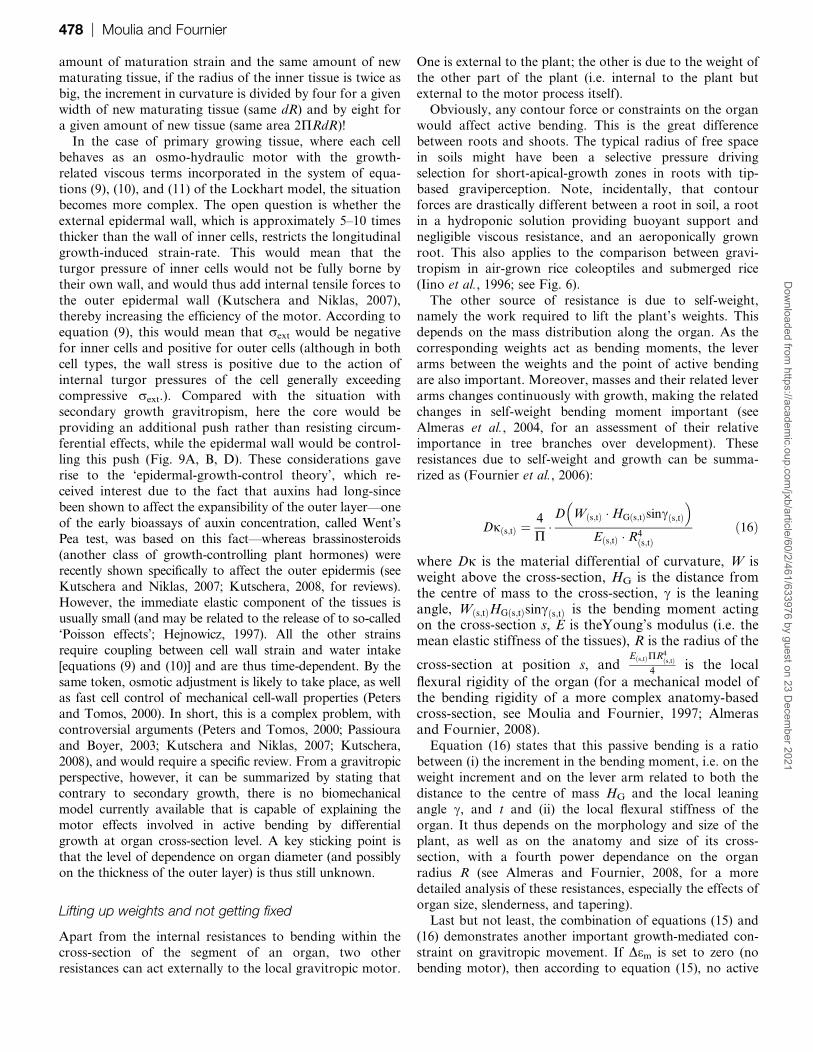
amount of maturation strain and the same amount of new

maturating tissue, if the radius of the inner tissue is twice as

big, the increment in curvature is divided by four for a given

width of new maturating tissue (same dR) and by eight for

a given amount of new tissue (same area 2PRdR)!

In the case of primary growing tissue, where each cell

behaves as an osmo-hydraulic motor with the growth-

related viscous terms incorporated in the system of equa-tions (9), (10), and (11) of the Lockhart model, the situation

becomes more complex. The open question is whether the

external epidermal wall, which is approximately 5–10 times

thicker than the wall of inner cells, restricts the longitudinal

growth-induced strain-rate. This would mean that the

turgor pressure of inner cells would not be fully borne by

their own wall, and would thus add internal tensile forces to

the outer epidermal wall (Kutschera and Niklas, 2007),thereby increasing the efficiency of the motor. According to

equation (9), this would mean that rext would be negative

for inner cells and positive for outer cells (although in both

cell types, the wall stress is positive due to the action of

internal turgor pressures of the cell generally exceeding

compressive rext.). Compared with the situation with

secondary growth gravitropism, here the core would be

providing an additional push rather than resisting circum-ferential effects, while the epidermal wall would be control-

ling this push (Fig. 9A, B, D). These considerations gave

rise to the ‘epidermal-growth-control theory’, which re-

ceived interest due to the fact that auxins had long-since

been shown to affect the expansibility of the outer layer—one

of the early bioassays of auxin concentration, called Went’s

Pea test, was based on this fact—whereas brassinosteroids

(another class of growth-controlling plant hormones) wererecently shown specifically to affect the outer epidermis (see

Kutschera and Niklas, 2007; Kutschera, 2008, for reviews).

However, the immediate elastic component of the tissues is

usually small (and may be related to the release of to so-called

‘Poisson effects’; Hejnowicz, 1997). All the other strains

require coupling between cell wall strain and water intake

[equations (9) and (10)] and are thus time-dependent. By the

same token, osmotic adjustment is likely to take place, as wellas fast cell control of mechanical cell-wall properties (Peters

and Tomos, 2000). In short, this is a complex problem, with

controversial arguments (Peters and Tomos, 2000; Passioura

and Boyer, 2003; Kutschera and Niklas, 2007; Kutschera,

2008), and would require a specific review. From a gravitropic

perspective, however, it can be summarized by stating that

contrary to secondary growth, there is no biomechanical

model currently available that is capable of explaining themotor effects involved in active bending by differential

growth at organ cross-section level. A key sticking point is

that the level of dependence on organ diameter (and possibly

on the thickness of the outer layer) is thus still unknown.

Lifting up weights and not getting fixed

Apart from the internal resistances to bending within the

cross-section of the segment of an organ, two other

resistances can act externally to the local gravitropic motor.

One is external to the plant; the other is due to the weight of

the other part of the plant (i.e. internal to the plant but

external to the motor process itself).

Obviously, any contour force or constraints on the organ

would affect active bending. This is the great difference

between roots and shoots. The typical radius of free space

in soils might have been a selective pressure driving

selection for short-apical-growth zones in roots with tip-based graviperception. Note, incidentally, that contour

forces are drastically different between a root in soil, a root

in a hydroponic solution providing buoyant support and

negligible viscous resistance, and an aeroponically grown

root. This also applies to the comparison between gravi-

tropism in air-grown rice coleoptiles and submerged rice

(Iino et al., 1996; see Fig. 6).

The other source of resistance is due to self-weight,namely the work required to lift the plant’s weights. This

depends on the mass distribution along the organ. As the

corresponding weights act as bending moments, the lever

arms between the weights and the point of active bending

are also important. Moreover, masses and their related lever

arms changes continuously with growth, making the related

changes in self-weight bending moment important (see

Almeras et al., 2004, for an assessment of their relativeimportance in tree branches over development). These

resistances due to self-weight and growth can be summa-

rized as (Fournier et al., 2006):

Djðs;tÞ ¼4

P�D�Wðs;tÞ �HGðs;tÞsincðs;tÞ

�Eðs;tÞ � R4

ðs;tÞð16Þ

where Dj is the material differential of curvature, W isweight above the cross-section, HG is the distance fromthe centre of mass to the cross-section, c is the leaningangle, Wðs;tÞHGðs;tÞsincðs;tÞ is the bending moment actingon the cross-section s, E is theYoung’s modulus (i.e. themean elastic stiffness of the tissues), R is the radius of the

cross-section at position s, andEðs;tÞPR4

ðs;tÞ4

is the local

flexural rigidity of the organ (for a mechanical model ofthe bending rigidity of a more complex anatomy-basedcross-section, see Moulia and Fournier, 1997; Almerasand Fournier, 2008).

Equation (16) states that this passive bending is a ratio

between (i) the increment in the bending moment, i.e. on the

weight increment and on the lever arm related to both the

distance to the centre of mass HG and the local leaning

angle c, and t and (ii) the local flexural stiffness of the

organ. It thus depends on the morphology and size of theplant, as well as on the anatomy and size of its cross-

section, with a fourth power dependance on the organ

radius R (see Almeras and Fournier, 2008, for a more

detailed analysis of these resistances, especially the effects of

organ size, slenderness, and tapering).

Last but not least, the combination of equations (15) and

(16) demonstrates another important growth-mediated con-

straint on gravitropic movement. If Dem is set to zero (nobending motor), then according to equation (15), no active


ownloaded from



ber 2021

change in curvature would occur. However, there is a change

in cross-sectional radius R. At the same time, growing weight

induces a passive down-bending according to equation (16).

If at some point, the regulatory system sets the bending

motor on again, then the work to recover from the passive

bending will be much higher due to the R inverse-square

dependence of the gravitropic motor (equation 15). This is

due to the fact that since newly-deposited cell wall layerstend to mould onto existing cell wall, there is a tendency for

curvature to become fixed by cell-wall deposition (see Fig. 6

in Moulia et al., 2006) in the absence of motor activity.

Thus, growth acts a double constraint on shape, through

down-bending and by fixing any curvature, so that without

active motor drivers and gravitropic regulation, any axis will

tend to droop down and weep (Moulia et al., 2006). This

conflict between the motor and fixing consequences ofgrowth is central to the actual shape of many organs

(Almeras et al., 2002, 2004; Coutand et al., 2007). It is thus

necessary to integrate both motor and resistances with

graviperceptive regulation into more complex models in

order to get a grasp on the power and control of movements.

Two integrative models of shootgravitropism

We have seen that the gravitropic response of an organ

involves (i) dose-sensitive sensing of the disorientation versus

gravity, and possibly other variables too (autotropism), (ii)

transduction of this response from the gravisensing cells tothe motor cells, (iii) size and anatomy-dependent biomechan-

ical motors, and (iv) internal and external resistances, all of

which act non-linearly. Directly handling the combination of

all these processes within quantitative arguments is beyond

the capacity of the human mind, but formalized models

provide suitable tools. Modelling has a long history in

gravitropic studies, and some of the equations involved in

such models have already been discussed in the previoussections (see Fournier et al., 1994a, and Meskauskas et al.,

1999a, b, for reviews). We will focus here on only two

models, selected for three reasons: (i) they are among the

most recently produced, (ii) they deal with spatial–temporal

changes in the curvature field, and (iii) they have been

compared with detailed experimentally-derived kinematic

data (Meskauskas et al., 1999a, b; Coutand et al., 2007).

Meskauskas’ model deals with gravitropism through primarygrowth, whereas Fournier’s model deals with gravitropism

through secondary growth. Yet besides their individual

interests, comparing the two provides key insights.

Fournier’s model was first published in 1994. More

complex versions have since been developed (Jirasek et al.,

2000; Fourcaud and Lac, 2003; Fourcaud et al., 2003;

Almeras et al., 2005; Almeras and Fournier, 2008), but the

central elements have remained unchanged. The gravitropicreaction is modelled through the following steps and

associated basic equations.

(i) Gravisensing is assumed be locally and uniformly

distributed along the stem according to the endodermal

starch-sheath theory and the experimental localization of

gravisensing (Weize et al., 2000). It displays a dose–response

to angle related to equation (7b), but in which the sensed

angle is the local angle c(s,t) and not the tip angle. This local

graviperception function is held to control the transverse

distribution of maturation strain Dem(s,t) through reaction

wood differentiation, with negligible lag-time i.e.

Demðs;tþdtÞ ��kSAðcðs;tÞ�cGSAÞjcðs;tÞ�cGSAj , with cGSA and kSA being con-

stants for the species. This equation is a simplification of

equation (7b), where only the sign of the angular distortion�cðs;tÞ � cGSA

�is sensed rather than its exact value.

(ii) The local bending PPS motor is modelled biomechan-

ically taking into account (i) positional effects of tissues laid

down by secondary growth within the cross-section, and (ii)

the internal resistance of the older core, using equation

(15b). The spatio-temporal distribution of secondary

growth DR/Dt (s,t) is an input to equation (15b) taken from

exogenous data (i.e. assuming no graviperception feedback

on the mean rate of secondary growth).

(iii) The resistive bending due to increments of self-weightalong the stem and of stem length is modelled using

equation (16) and taking into account the detailed shape of

the stem. The primary growth dL/dt (where L is total

length) and its orientation are taken from exogeneous data.

(iv) The distribution of local inclination angles c(s,t+dt) is

then computed from change in curvature Dj/Dt(s,t), using

spatial integration [equation (2), solved for every position s].

This step requires boundary angular conditions at the base

and the tip of the organ. Anchorage is usually assumed to

be perfectly stiff (no angular variation of the stem base).

The apical primary growing segment is assumed to have

achieved its orientation according to cGSA within one time-

step (since primary gravitropism is much faster than

secondary gravitropism).

Note that this model only has one parameter (kSA) to be

fitted (on an independent dataset); all the other values can

be measured directly and independently of the model

(although in some studies, some of them were also

estimated to avoid overcrowding the measurements). Up to

now, growth data (radial and apical growth) are inputs

issued from (i) experimental data (Coutand et al., 2007) or

(ii) independent growth models (assuming no feedback of

graviperception on the mean rates of growth).

This type of model has proved to be able to account for

the S-shape of certain branches (Fournier et al., 1994a;

Jirasek et al., 2000) without the need to assume ad hoc

variations in GSA cGSA, as was the case previously (Digby

and Firn, 1995). This S-shape is simply due to mechanical

competition over time between the downward drooping due

to changes in self-weight increasing the lever arm toward

the base, and the setting of primary growth direction on the

apical zone of the branch and/or the onset of the reaction

wood motor and active geotropic reorientation. This explan-

atory model was assessed experimentally and was found to

agree with measured data as long as the Young’s modulus

was correctly estimated (Almeras et al., 2002). It should be

noted that the model was also able to simulate very different


ownloaded from



ber 2021

rates of curvature changes Dj/Dt(s,t) as a function of position

s along the organ, despite a similar graviperceptive function.

This is because the local rate of change in curvature depends

on stem radius, which usually varies significantly along the

stem, especially in woody plants. Indeed, for the motor

bending, equation (15) shows that the gravitropic curvature

rate scales as R�2(s,t). Thus, even when everything else is

kept constant along the stem in equation (15) (stimulationangle, radial growth dR(s,t), cross-section shape, maturation

strain, and Young’s modulus distribution), the rate of

curvature Dj/Dt(s,t) is greatly influenced by the taper [i.e. the

variations of the radius R(s) along the stem positions).

Actually, Dj/Dt(s,t) will be significantly lower in the distal

thicker parts of the stem. For example, a realistic taper of

1 cm m�1 in equation (15) produces a decrease of the

curvature rate of 1 � 12

22 ¼ 75% between a 1 cm thick segmentand a 2 cm thick one located 1 m below.

In addition, the taper R(s,t) is not usually constant over

time during growth. The observed curvature rate Dj/Dt(s,t)

then comes as the superimposition of the motor bending

(equation 15) and the resistive bending due to selfweight

growth [equation (16)]. Therefore, the variations along the

stem of the curvature rate should be more complex than

a simple R–2(s,t) function, although always greatly influ-enced by taper and size. Without a proper analysis of these

effects of size and shape using biomechanical models, there

is a high risk of interpreting purely biomechanical con-

sequences of stem geometry on the rate of changes in

curvature as biological differences of gravisensing and

dose–response functions. This risk is heightened if only the

changes in tip angle as a function of its previous inclination

angle are monitored (as the tip angle results from thesummation of the changes in curvature from s¼0 to

s¼L—see equation (2)—and is thus dependent on L and on

the overall shape of the stem; Fig. 3F). This clearly

demonstrates how any attempt to infer differences in

gravisensitivity (and/or in GSA) without a good knowledge

of the biomechanics of the motor forces and resistances

involved can yield very misleading results.

Despite its good predictive behaviour, Fournier’s integra-tive model was recently falsified using a detailed kinematical

study of curvature field and growth in poplar trees

(Coutand et al., 2007). Some of the discrepancy between

the model and the experimental data was due to insufficient

knowledge on the kinetics of maturation Dm(x,y,s,t). But the

major discrepancy was that the model tended to overshoot

whereas the real tree never did (see Fig. 5). This discrepancy,

which arose mainly from the gravisensing control in themodel, clearly pointed towards a more complex control on

bending rates than that due to the sine law of gravisensing.

A similar conclusion was reached by Meskauskas and

coworkers working with primary organs (Meskauskas and

Moore, 1998; Meskauskas et al., 1999b) but using more

advanced models of graviperception. Consistent with the

experimental data on auxin transport, they initially pro-

posed a model combining gravisensing of (i) the tip anglecT(t) according to the sine law equation (7) ST(t)¼sin(cT(t))

and (ii) the local angle c(s,t). Several laws for the gravisens-

ing of the local angle have been tested (Meskauskas and

Moore, 1998; Meskauskas et al,. 1999a), and a negative

exponential law SLðs;tÞ ¼ e�kSL�ðP2 � cðs;tÞÞ was the one retained

(although no mechanistic grounds in terms of cellular

gravisensing could be given up until then). For the two

perceptions to act locally at the same s would require a signal

transmission from the tip. After testing several transmission

laws against experimental data (Meskauskas and Moore,1998), they ended with a wave transmission at velocity mT

with an exponential decrease in magnitude as it progresses

downward STðs;tÞ ¼ STðt�ð1�s=LÞ=vTÞ � e�kTð1�s=LÞ (Meskauskas

et al., 1999a). It was assumed that the two signals act

additively on the differential growth response, i.e.

Xðs;tÞ ¼ SLðs;tÞ þ STðs;tÞ ¼ SLðs;tÞ þ STðt�ð1�s=LÞ=vTÞ � e�kTð1�s=LÞ.No biomechanical modelling of the differential-growth

motor was proposed, since, as explained in the previoussection, none is yet available. Therefore a direct relationship

between the rate of curvature change at position s and the

dual gravisensing signal X(s,t) was assumed. As in Four-

nier’s model, the distribution of local inclination angles

c(s,t+dt), including the tip angle cT(t), was computed from the

change in curvature, using spatial integration [equation (2),

solved for every position s]. However, when tested against

experimental data, this model turned out to be clearlyinsufficient (as did all of the other combinations of trans-

mission laws and local perceptive laws; Meskauskas et al.,

1999b). Three additional ingredients had to be added:

(i) First of all, and principally, an autotropic curvature-

compensation mechanism based on curvature sensing (in-

dependently of the gravisensing of inclination) has to be

included, i.e. Aðs;tÞ ¼ kA � jðs;tÞ to make:

X�s; t

�¼ SLðs;tÞ þ STðs;tÞ þ Aðs;tÞ ð17Þ

This is why Meskauskas and coworkers named theirmodel the ‘revised local curvature distribution model’.

(ii) Furthermore, a non-uniform capacity for local sensing

of both curvature and local angle had to be retained (bothwere assumed to decrease exponentially from the apex in

a basipetal direction).

(ii) Finally, a multiplicative realization coefficient Kw had

to be added (probably accounting for the efficiency of the

unmodelled motor mechanism in working the active bending).

Using this new set of equations, Meskauskas et al. were

able to reproduce experimental situations that were not part

of the context used to design the model, including responsesto different initial angles c0 (this was not the case for older

models). They were also able to reproduce the fact that

gravireacting stems may straighten before overshooting the

vertical, and may also reach a steady inclination that is not

the vertical without having to introduce an ad hoc time-

changing GSA. Moreover, this model turned out be

relatively generic, able to fit responses of organisms as

different as the Coprinus stipe and the wheat coleoptile

(Meskauskas et al., 1999a, b). Last but not least, the model

could also fit the responses of stems submitted to physio-

logical inhibitors of the gravisensing pathway (i.e. a Ca2+

chelator, a Ca2+ ionophore, and an inhibitor of the


ownloaded from



ber 2021

cytoskeleton formation of F-actin filaments), making it

feasible for use as a reverse tool for estimating quantitative

physiological effects (Meskauskas et al., 1999a).

There are several limitations to the Meskauskas ‘revisedlocal curvature distribution model’. One is obviously that it

features nine parameters whose estimations can only be

achieved using the model. From a statistical perspective of

parameter estimation, this is a lot. It becomes necessary to

design very large datasets derived from a set of experiments

planned to act almost orthogonally on the parameters in the

model, so that the estimates of the various parameters are

not too correlated. Otherwise, even when the model appears

to fit the data well, it could still be due to numerical

compensatory artefacts between the parameter values

(Tremblay and Wallach, 2004). Despite fitting the model on

four cleverly chosen experiments, the current dataset

studied by Meskauskas and co-workers does not yet appear

sufficiently comprehensive, and there may be a great deal of

experimental work to do. That said, if the model could be

made less complex, or at least made to use parameters that

can be directly measured independently of the model, it

would become easier to assess and be extremely useful. The

comparison with Fournier’s model here may be informative.

Meskauskas and co-workers had to model in a decrease in the

ability to respond to local sensing of both curvature and local

angle, together with a realization coefficient Kw for the curving

(i.e. three additional parameters). However, this apparent

decrease in curving response along the axis may result from

differences in the balance between motor efficiency and

mechanical resistance levels all along the organ (as they are

known to be diameter and lever-arm-dependent) rather than

on ad hoc variations in local sensitivities. Including a bio-

mechanical model of both motors and resistances would

make it possible to replace these ad hoc parameters with

biophysical parameters that can be measured directly.The second limitation of the Meskauskas’ model is that it

does not, in its present state, take into account the

kinematics of expansion growth, as only the local time-

derivative@jðs;tÞ@t was considered instead of the material

derivativeDjðs;tÞDt

[thus neglecting convective changes that

were likely to occur due to clear curvature gradients@jðs;tÞ@s ;

see equation (3)]. Some acknowledgement of the effect of

expansion growth as introduced by using the relative cur-

vilinear abscissa s/L rather than the absolute value s in the

terms of exponential spatial decrease in the three signals, but

this is still insufficient, as (i) expansion growth is spatially

non-uniform and (ii) the convective effects might be strong.

Despite their limitations (and it is normal for scientific

advance that state-of-the-art models are criticized and

eventually falsified), taken together, these two models bring

a clear convergent perspective.First of all, the autotropic curvature-compensation mech-

anism is central to the overall gravitropic-straightening

response (Iino, 2006; Moulia et al., 2006). It is not possible

to reach the vertical through bending, and so counter-

bending is necessary in order to get straight. Moreover,

autotropic curvature sensing acts concomitantly with grav-

isensing, and both drive the bending motor. As soon as

gravitropic curvature starts, autotropic curvature compen-

sation is activated. Therefore, only the very initial rate of

curvature changes may actually be measuring the response

to gravisensing, but to be measured accurately requires

highly sensitive spatio-temporal kinematical measurements,

such as the recent bio-imaging methods. Estimates of angles

such as the one shown in Fig. 2A are clearly a measure ofthe steady balance between gravitropic and autotropic

sensing (Meskauskas et al., 1999b), and do not serve to

characterize gravisensitivity.

Second, it is not possible to analyse gravisensitivity and

its possible changes during the graviresponse without

considering (i) the distribution of the curvature response

(and of the growth response), and (ii) without having a good

estimation of the powers of the motor and of the variousresistances, as these depend biomechanically on cross-

sectional size and anatomy, as well as on organ length and

specific weight. Only then does it become possible to tackle

the important issues of varying sensitivity and possible

accommodation (Moulia et al., 2006) of the gravi- and

mechano-sensing system. A good example of a model pro-

viding direct access to local gravisensitivity is the work by

Yamashita et al. (2007) in tree stems. As shown previously,the gravitropic response is mediated by reaction wood

formation according to the PPS motor and Fournier’s model

[equations (15) and (16)], and the variable controlled by

gravisensing is maturation strain Dem. Yamashita et al. (2007)

maintained the stem attached to a stiff stake. This confers

three advantages. The most obvious is that the stimulation

angle c is maintained constant and the presentation time tscan be controlled. But there is more. Using the biomechanicalmodel of the motor and the resistance to bending, it can be

shown that restraining any bending results in an override of

the resisting effects of the inner core and the self-weight, so

that a very accurate estimation of the Dem input to the PPS

motor can be measured directly. An accurate local dose–

response curve could thereby be determined for the gravi-

tropic motor input. The authors found that maturation

strains increased for stimulation angles c smaller than 30�and then saturated, a function differing from a sine law and

radically different from a negative exponential.

Third, formalized models integrating physiological and

mechanical processes are highly useful tools for handling

and analysing the complexity of organ response. Gravitrop-

ism is a feedback process where current geometrical

configuration is sensed and influences the next step. Too

much focus on the so-called initial phases is likely to hindersome very significant mechanisms (even the gravisensing

mechanism itself). This might be highly detrimental when

analysing physiological responses such as that of inhibitors,

or when phenotyping mutants. Consider the case of

mutants or inhibitors affecting cytoskeleton dynamics

(Palmieri et al., 2007). Cytoskeleton dynamics is known

potentially to affect statolith movements (Morita and

Tasaka, 2004), mechanosensing (Perbal and Driss-Ecole,2003), PIN relocalization, cell wall growth (Ikushima et al.,

2008), and the list could well go on! Using integrative


ownloaded from



ber 2021

models and related experiments, it might be possible

quantitatively to analyse the individual contributions of

these effects to the overall gravitropic phenotype (Meskaus-

kas et al., 1999b; Moulia et al., 2006).

To round up, integrative models can be used to analyse

the effect of genetic variation in the parameter values (due

to natural quantitative variations, mutations, or genetic

engineering) for phenotypic performance (Tardieu, 2003).This leads us to our last point, namely the ecological

significance of gravitropism.

Back to the HMS Beagle: natural diversity inshoot gravitropism and its adaptivesignificance

It is usually considered that a major motivation for Charles

Darwin in his studies following ‘On the origin of species’ was

to study the natural variation of traits in living beings and

to gain further insights into possible natural selection.

Indeed, ‘The power of movement in plants’, studied manydifferent species. It is, however, striking that, until only

recently, very little consideration had been given to the

ecological significance of variations in gravitropism re-

sponse. This is probably because focus was given solely to

the obvious role of gravitropism in seedlings. In ‘The power

of movement in plants’, the ecological function of gravitrop-

ism is dealt with in the Introduction, stating basically that

gravitropisms make it possible for the seedling shoot to findits way up, even if it is buried in the soil, and for the radicle

to find its way down into the soil. More efficiency in this

process might affect germination success, but this is only

one of the many environmental selective pressures acting on

seedling survival (Coomes and Grubb, 2003). Although

often noted in passing, the life-long central importance of

gravitropism and autotropism in land-growing plants has

only recently been stressed (Mosbrugger, 1990; Iino et al.,2006; Moulia et al., 2006; Almeras and Fournier, 2008).

Indeed, gravi-autotropism provides the plant with (i) the

ability to regulate posture and (ii) the ability actively to

recover from non-lethal mechanical hazards such as moder-

ate windthrow, soil slipping, or mechanical buckling under

self-weight (Moulia et al., 2006). Different species or

different plant stages might involve different motors, but

all land-erected plants have the power of movement throughan active motor (actually, in most plants, several motors

can act simultaneously; Hay et al., 2000; Moulia et al.,

2006). Moreover, it has been proposed that the adaptive

significance of gravi-auto-tropisms is linked to the mechan-

ical dimensioning of the plant body through thigmomor-

phogenesis (Moulia et al., 2006) and photomorphogenesis

(Fournier et al., 2006). Thigmomorphogenesis is the central

process in adapting the plant’s mechanical structure to fit itsmechanical environment (wind, slope, self-weight, etc.).

Gravi-autotropic recovery plays a particularly important

role when plants have to undertake risks, either by growing

tall and thin under dim light to reach the canopy (Fournier

et al., 2006; Iino, 2006) or by suddenly having to cope with

much more wind drag when overtopping other plants (de

Langre, 2008).

It has been shown that there is considerable interpecific

variability in the performances of the gravisensing systems.

Variations of one order of magnitude in the apparent

presentation time sp between species have been reported

(Audus, 1969), ranging from less than a minute up to

several hours. More recently, ecotypic variations have alsobeen described. Considering the inflorescence stems of

Arabidopsis grown under the same controlled conditions,

Tanimoto et al. (2008) reported that most of the amylo-

plasts reached the apical side of statocytes within 20 min in

the Col ecotype compared to 60 min in Ler, which equates

to a factor of 3 in presentation times. Sierra et al. (2008)

demonstrated that ecotypes of pine (Pinus pinaster Ait)

displayed very large differences in gravitropic efficiency(due to differences in the response of the differential

maturation strain to inclination angle) as well as in their

autotropic capacity. High gravitropic motor and auto-

tropic control efficiencies yielded much improved adult

trunk straightness in provenance trials, giving rise to

interesting selection criteria for plant breeding (and maybe

for natural selection?). Note, incidentally, that this analysis

in Sierra et al. (2008) was achieved using integrativebiomechanical models.

Lastly, Fournier et al. (2006), studying the communities

with the highest biodiversity on Earth, the rain forests,

demonstrated through extensive surveys on a community of

tree species that 92% of sapling stems display active

gravitropic movement either compensating (9%) or over-

topping (81%) growth-induced downward-drooping, high-

lighting the prevalence of gravitropic control. Since thereare still no available long-term kinematical studies on trees

(which, by definition, would have to run over decades), this

analysis employed integrative biomechanical models. More-

over, the very large interspecific variation in in situ

gravitropic performance and in gravitropic capacity in

optimally-controlled environments could be correlated with

the amount of mechanical risk the species faces in its

environment. This clearly raises the possibility of integratedbiomechanical strategies for height growth in land plants

(Fournier et al., 2006; Moulia et al. 2006). The significance

of this in terms of functional land ecosystem ecology and

evolutionary biology (Mosbrugger, 1990) has yet to be

studied, but there is no doubt that integrative biomechani-

cal models will provide pivotal input by helping define

relevant ‘hard’ process-based traits and estimating them in

large populations (Fournier et al., 2006; Sierra et al., 2008).However, this would also require a more concerted

ecological research effort covering various situations, but

can be expected to bring many insights (Fournier et al.,

2006; Iino, 2006), just as HMS Beagle’s journey was

instrumental to Charles Darwin’s work.

Conclusion

Over almost 130 years, huge advances have been made in

our understanding of gravitropic movement in plants. We


ownloaded from



ber 2021

have gained a great deal of insight into the underlying

molecular mechanisms, and biomechanical studies together

with spatial microgravity studies have revealed the role

played by physics in the process. Nevertheless, in the

context of this review, it is striking to see how far the

current explanatory models and tools can be traced back to

Darwins’ time: examples include the starch-statolith hy-

pothesis, osmo-hydraulic motors, and growth kinematics, toname but a few.

To some extent, though, the last few decades have been

characterized by discipline segmentation and increasingly

specialized studies. This has clearly been rewarding, as the

process has produced efficient tools and numerous facts that

have pushed back the boundaries of plant physiology.

However, limits to this segmentation may now have been

reached. There are clear needs and rewards for interdisciplin-ary approaches involving modern physics and biology in the

field of gravitropism; some of the insights already brought by

such approaches have been presented in this review. Mathe-

matical modelling coupled with high-resolution bio-imaging

are proving to be powerful tools, and can be expected to drive

gravitropic studies into the realm of modern systems biology.

Modelling has turned out to be a more accurate way of

setting and testing hypotheses dealing with the non-lineardynamic systems involved in gravitropism, as long as these

models are assessed continuously with crucial experiments.

Integrative models are also likely to be extremely helpful in

evaluating and rating the efficiency of the control of a given

gene on the overall performance of the shoot. They also

therefore lend themselves perfectly to phenotyping plant

gravitropic mutants, and to defining relevant gravitropic

traits for ecological study.Our review on the state-of-the-art in gravitropic model-

ling has revealed at least four domains where the de-

velopment of integrative biomechanical modelling would

offer rewards: (i) integrative models of cellular gravisensing,

including statoliths and their collective dynamics as well as

their interactions with molecular motors and vesicular traffick-

ing; (ii) integrative models of the primary bending motor, and

of its genetic controls; (iii) models of the interplay betweengravitropism and autotropism (and phototropism) in the

control of gravitropic movement and the signalling required

for it to be co-ordinated in a given organ as well as across the

entire plant architecture (Trewavas, 2003; Moulia et al., 2006;

Fourcaud et al., 2008), and (iv) population and community

models in ecology, analysing the significance of genetic

variation in gravitropism and, more generally, the significance

of biomechanical height growth strategies in ecosystemfunction and, ultimately, for the fitness of plant species in

different environments. This more integrated and interdisci-

plinary view might take us deeper into the research agenda on

the power of movement in plants and its ecological signifi-

cance, an agenda originally drawn 150 years ago.

Acknowledgements

We thank Dr C Girousse and R Bastien for reading the ms,

Mr McCulley from A-T-T (http://www.a-t-t.fr), for care-

fully proof-reading the ms for the English, and an

anonymous reviewer for useful suggestions. This work has

been supported by ANR-05-BDIV-012-03 ‘Woodiversity’.

References

Almeras T, Costes E, Salles JC. 2004. Identification of biomechan-

ical factors involved in stem shape variability between apricot tree

varieties. Annals of Botany 93, 455–468.

Almeras T, Fournier M. 2008. Biomechanical design and long-term

stability of trees: morphological and wood traits involved in the balance

between weight increase and the gravitropic reaction. Journal of

Theoretical Biology (in press).

Almeras T, Gril J, Costes E. 2002. Bending of apricot tree branches

under the weight of axillary growth: test of a mechanical model with

experimental data. Trees 16, 5–15.

Almeras T, Thibaut A, Gril J. 2005. Effect of circumferential

heterogeneity of wood maturation strain, modulus of elasticity and radial

growth on the regulation of stem orientation in trees. Trees 19, 457–467.

Almeras T, Yoshida M, Okuyama T. 2006. Generation of longitudi-

nal maturation stress is not related to diurnal changes in diameter.

Journal of Wood Science 52, 452–455.

Archer RR. 1987. Growth stresses and strains in trees. Berlin: Springer.

Audus LJ. 1964. Geotropism and the modified sine rule; an

interpretation based on the amyloplast statolith theory. Physiologia

Plantarum 17, 737–745.

Audus LJ. 1969. Geotropism. In: Wilkins MB, ed. The physiology of

plant growth and development. London: McGraw-Hill, 203–241.

Basu P, Pal A, Lynch JP, Brown KM. 2007. A novel image-analysis

technique for kinematic study of growth and curvature. Plant

Physiology 145, 305–316.

Ben Amar M, Goriely A. 2005. Growth and instability in elastic tissues.

Journal of the Mechanics and Physics of Solids 53, 2284–2319.

Bennett MJ, Roberts J, Palme K. 2000. Moving on up: auxin-

induced K+ channel expression regulates gravitropism. Trends in Plant

Science 5, 85–86.

Blancaflort EB, Masson PH. 2003. Plant gravitropism. Unraveling the

ups and downs of a complex process. Plant Physiology 133, 1677–1690.

Boyer JS, Silk WK. 2004. Hydraulics of plant growth. Functional

Plant Biology 31, 761–773.

Burgert I, Eder M, Gierlinger N, Fratzl P. 2007. Tensile and

compressive stresses in tracheids are induced by swelling based on

geometrical constraints of the wood cell. Planta 226, 981–987.

Chavarria-Krauser A. 2006. Quantification of curvature production in

cylindrical organs, such as roots and hypocotyls. New Phytologist 171,

633–641.

Chavarria-Krauser A, Nagel KA, Palme K, Schurr U, Walters A,

Scarr H. 2008. Spatio-temporal quantification of differential processes

in root growth zones based on a novel combination of image

sequence processing and refined concepts describing curvature

production. New Phytologist 177, 811–821.

Clair B, Almeras T, Sugiyama J. 2006. Compression stress in

opposite wood of angiosperms: observations in chestnut, mani and

poplar. Annals of Forest Science 63, 507–510.


ownloaded from



ber 2021

http://www.a-t-t.fr

Clair B, Almeras T, Yamamoto H, Okuyama T, Sugiyama J. 2007.

Mechanical behavior of cellulose microfibrils in tension wood, in relation

with maturation stress generation. Biophysical Journal 91, 1128–1135.

Coen E, Rolland-Lagan AG, Matthews M, Bangham JA,

Prusinkiewicz P. 2004. The genetics of geometry. Proceedings of

the National Academy of Sciences, USA 101, 4728–4735.

Coomes DA, Grubb PJ. 2003. Colonization, tolerance, competition

and seed-size variation within functional groups. Trends in Ecology

and Evolution 18, 283–291.

Correll MJ, Kiss JZ. 2008. Space-based research on plant tropisms.

In: Gilroy S, Masson PH, eds. Plant tropisms. Oxford, UK: Blackwell

Publishing, 161–182.

Cosgrove DJ. 1990a. Rapid, bilateral changes in growth rate and

curvature during gravitropism of cucumber hypocotyls: implications for

mechanisms of growth control. Plant, Cell and Environment 13, 227–234.

Cosgrove DJ. 1990b. Gravitropism of cucumber hypocotyls: bio-

physical mechanism of altered growth. Plant, Cell and Environment

13, 235–241.

Coutand C, Fournier M, Moulia B. 2007. Gravitropic response of

polar trunk: key roles of the regulation of wood prestressing and of

relative kinetics of cambial growth versus wood maturation. Plant

Physiology 144, 1166–1180.

Coutand C, Moulia B. 2000. Biomechanical study of the effect of

a controlled bending on tomato stem elongation. II. Local strain

sensing and spatial integration of the signal. Journal of Experimental

Botany 51, 1825–1842.

Darwin C, Darwin F. 1880. The power of movements in plants.

London, England: Murray.

de Langre E. 2008. Effects of wind on plants. Annual Review of Fluid

Mechanics 40, 141–168.

Digby J, Firn RD. 1995. The gravitropic set-point angle (GSA): the

identification of an important developmentally controlled variable gov-

erning plant architecture. Plant, Cell and Environment 18, 1434–1440.

Dolk H. 1936. Geotropism and the growth substance. Recueil des

Travaux Botaniques Neerlandais 33, 509–585.

Du S, Yamamoto F. 2007. An overview of the biology of reaction

wood formation. Journal of Integrative Plant Biology 49, 131–143.

Dumais J, Shaw SL, Steele CR, Long SR, Ray PM. 2006. An

anisotropic-viscoplastic model of plant cell morphogenesis by tip

growth. International Journal of Developmental Biology 50, 209–222.

Edwards CH, Penney DE. 1994. Calculus with analytical geometry.

New Jersey, USA: Prentice Hall, Englewoods Cliffs.

Firn RD, Digby J. 1979. A study of autotropic straightening reaction

of a shoot previously curved during geotropism. Plant, Cell and

Environment 2, 149–154.

Firn RD, Digby J. 1980. The establishment of tropic curvatures in

plants. Annual Review of Plant Physiology 31, 131–148.

Firn RD, Digby J, Hall LA. 1981. The role of the shoot apex in

geotropism. Plant, Cell and Environment 4, 125–129.

Fourcaud T, Blaise F, Lac P, Castera P, Reffye Pd. 2003.

Numerical modelling of shape regulation and growth stresses in trees.

II. Implementation in the AMAPpara software and simulation of tree

growth. Trees: Structure and Function 17, 31–39.

Fourcaud T, Lac P. 2003. Numerical modelling of shape regulation

and growth stresses in trees. I. An incremental static finite element

formulation. Trees: Structure and Function 17, 23–30.

Fourcaud T, Zhang X, Stokes A, Lambers H, Korner C. 2008.

Plant growth modelling and applications: the increasing importance of

plant architecture in growth models. Annals of Botany 101, 1053–1063.

Fournier M, Bailleres H, Chanson B. 1994a. Tree biomechanics:

growth, cumulative prestresses and re-orientations. Biomimetics 2,

229–251.

Fournier M, Chanson B, Thibaut B, Guitard D. 1994b. Measure-

ments of residual growth strains at the stem surface: observations on

different species. Annals of Forest Science 51, 249–266 (in French).

Fournier M, Stokes A, Coutand C, Fourcaud T, Moulia B. 2006.

Tree biomechanics and growth strategies in the context of forest

functional ecology. In: Herrel A, Speck T, Rowe N, eds. Ecology and

biomechanics: a biomechanical approach of the ecology of animals and

plants. Boca Raton, Florida, USA: CRC Taylor and Francis, 1–33.

Fukaki H, Fujisawa H, Tasaka M. 1996. Gravitropic response of inflo-

rescence stems in Arabidopsis thaliana. Plant Physiology 110, 933–943.

Galland P. 2002. Tropisms of Avena coleoptiles: sine law for

gravitropism, exponential law for photogravitropic equilibrium. Planta

215, 779–784.

Gilroy S, Masson PH. 2008. Plant tropisms. Oxford, UK: Blackwell

Publishing.

Girousse C, Moulia B, Silk W, Bonnemain JL. 2005. Aphid

infestation causes different changes in carbon and nitrogen allocation

in alfalfa stems as well as different inhibitions of longitudinal and radial

expansion. Plant Physiology 137, 1474–1484.

Haga K, Iino M. 2006. Asymmetric distribution of auxin correlates with

gravitropism and phototropism but not with autostraightening (autotrop-

ism) in pea epicotyls. Journal of Experimental Botany 57, 837–847.

Harisson BR, Morita MT, Masson PH, Tasaka M. 2008. Signal

transduction in gravitropism. In: Gilroy S, Masson PH, eds. Plant

tropisms. Oxford, UK: Blackwell Publishing, 21–46.

Haswell ES. 2003. Gravity perception: how plants stand up for

themselves. Current Biology 13, R761–R763.

Hay J, Moulia B, Silk WK, Lane B, Freeling M. 2000. Bio-

mechanical analysis of the rolled (Rld) leaf phenotype of maize.

American Journal of Botany 87, 625–633.

Hejnowicz Z. 1997. Graviresponses in herbs and trees: a major role for

the redistribution of tissue and growth stresses. Planta 203, S136–S146.

Hoshino T, Miyamoto K, Ueda J. 2007. Gravity-controlled

asymmetrical transport of auxin regulates a gravitropic response in the

early growth stage of etiolated pea (Pisum sativum) epicotyls: studies

using simulated microgravity conditions on a three-dimensional clinostat

and using an agravitropic mutant, ageotropum. Journal of Plant

Research 120, 619–628.

Hughes-Hallet D, Gleason AM, Frazer Lock P, Flath DE,

Gordon SP, Lomen DO, Lovelock D, McCallum WG,

Osgood BG, Pasquale A. 1996. Applied calculus: for business,

social sciences and life sciences. NY, USA: John Wiley & Sons.

Iino M. 2006. Toward understanding the ecological functions of

tropisms: interactions among and effects of light on tropisms. Current

Opinion in Plant Biology 9, 89–93.


ownloaded from



ber 2021

Iino M, Tarui Y, Uematsu C. 1996. Gravitropism of maize and rice

coleoptiles: dependence on the stimulation angle. Plant, Cell and

Environment 19, 1160–1168.

Ikushima T, Shimmen T. 2005. Mechano-sensitive orientation of

cortical micrtotubules during gravitropism in azuki bean epicotyls.

Journal of Plant Research 118, 19–26.

Ikushima T, Soga K, Hoson T, Shimmen T. 2008. Role of

xyloglucan in gravitropic bending of azuki bean epicotyl. Physiologia

Plantarum 132, 552–565.

Jirasek C, Prusinkiewicz P, Moulia B. 2000. Integrating bio-

mechanics into developmental plant models expressed using Lsys-

tems. In: Spatz H-C, Speck T, eds. Plant biomechanics, 2000. Third

Plant Biomechanics Conference. Freiburg, Germany: Thieme Verlag,

Stuttgart, Germany, 615–624.

Johansen JN, Vernhettes S, Hofte H. 2006. The ins and outs of

plant cell walls. Current Opinion in Plant Biology 9, 616–620.

Kiss JZ. 2000. Mechanisms of the early phases of plant gravitropism.

Critical Reviews in Plant Sciences 19, 551–573.

Krupkova E, Immerzeel P, Pauly M. 2007. The TUMOROUS

SHOOT DEVELOPMENT2 gene of Arabidopsis encoding a

putative methyltransferase is required for cell adhesion and

co-ordinated plant development. The Plant Journal 50, 735–750.

Kutschera U. 2001. Gravitropism of axial organs in multicellular

plants. Advances in Space Research 27, 851–860.

Kutschera U. 2008. The pacemaker of plant growth. Trends in Plant

Science 13, 105–107.

Kutschera U, Niklas KJ. 2007. The epidermal-growth-control theory

of stem elongation: an old and a new perspective. Journal of Plant

Physiology 164, 1395–1409.

LaMotte CE, Pickard BG. 2004. Control of gravitropic orientation. I.

Non-vertical orientation by primary roots of maize results from decay of

competence for orthogravitropic induction. Functional Plant Biology 31,

93–107.

Larsen P. 1969. The optimum angle of geotropic stimulation and its

relation to the starch statolith hypothesis. Physiologia Plantarum 22,

469–488.

Lockhart JA. 1965. An analysis of irreversible plant cell elongation.

Journal of Theoretical Biology 8, 264–275.

Mellerowicz EJ, Sundberg B. 2008. Wood cell walls: biosynthesis,

developmental dynamics and their implications for wood properties.

Current Opinion in Plant Biology 11, 293–300.

Meskauskas A, Moore D. 1998. Mathematical modelling of

morphogenesis in fungi. 1. Spatial organization of the gravitropic

response in the mushroom stem of Coprinus cinereus. New

Phytologist 143, 387–399.

Meskauskas A, Jurkoniene S, Moore D. 1999a. Spatial organiza-

tion of the gravitropic response in plants: applicability of the revised

local curvature distribution model to Triticum aestivum coleoptiles.

New Phytologist 140, 111–123.

Meskauskas A, Moore D, Novak Frazier LA. 1999b. Mathematical

modelling of morphogenesis in fungi. 2. A key role for curvature

compensation (‘autotropism’) in the local curvature distribution model.

New Phytologist 143, 387–399.

Miyamoto K, Katsuhara M, Ookawa T, Kasamo K, Hirasawa T.

2005. Hydraulic conductivity and aquaporins of cortical cells in

gravitropically bending roots of Pisum sativum L. Plant Production

Science 8, 515–524.

Morita MT, Tasaka M. 2004. Gravity sensing and signalling. Current

Opinion in Plant Biology 7, 712–718.

Mosbrugger V. 1990. The tree habit in land plants. A functional

comparison of trunk constructions with a brief introduction into the

biomechanics of trees. In: Bhattacharji SF, Gerald M, Neugebauer HJ,

Seilacher A, eds. Lecture notes in earth sciences, Vol. 28. Berlin,

Heidelberg: Springer-Verlag, 158.

Moulia B. 2000. Leaves as shell structures: double curvature,

autostresses and minimal mechanical energy constraints on leaf rolling

in grasses. Journal of Plant Growth Regulation 19, 19–30.

Moulia B, Coutand C, Lenne C. 2006. Posture control and skeletal

mechanical acclimation in terrestrial plants: implications for mechanical

modeling of plant architecture. American Journal of Botany 93,

1477–1489.

Moulia B, Fournier M. 1997. Mechanics of the maize leaf:

a composite beam model of the midrib. Journal of Materials Science

32, 2771–2780.

Moulia B, Fournier M, Guitard D. 1994. Mechanics and form of the

maize leaf: in vivo qualification of the flexural behaviour. Journal of

Materials Science 29, 2359–2366.

Muday GK, Rahman A. 2008. Auxin transport and the integration of

gravitropic growth. In: Gilroy S, Masson PH, eds. Plant tropisms.

Oxford, UK: Blackwell Publishing, 47–78.

Mullen JL, Ishikawa H, Evans ML. 1998. Analysis of changes in

relative elemental growth rate patterns in the elongation zone of

Arabidopsis roots upon gravistimulation. Planta 206, 598–603.

Myers AB, Glyn GH, Digby J, Firn RD. 1995. The effect of

displacement angle on the gravitropic and autotropic growth

responses of sunflower hypocotyls. Annals of Botany 75, 277–280.

Nakamura M, Negishi Y, Funada R, Yamada M. 2001. Sediment-

able amyloplasts in starch sheath cells of woody stems of japanese

cherry. Advances in Space Research 27, 957–960.

Ortega JKE. 1994. Plant and fungal cell growth: governing

equations for cell wall extension and water transport. Biomimetics 2,

215–228.

Palmieri M, Schwind MA, Stevens MHH, Edelmann RE, Kiss JZ.

2007. Effects of the myosin ATPase inhibitor 2,3-butanedione

monoxime on amyloplast kinetics and gravitropism of Arabidopsis

hypocotyls. Physiologia Plantarum 130, 613–626.

Passioura JB, Boyer JS. 2003. Tissue stresses and resistance to

water flow conspire to uncouple the water potential of the epidermis

from that of the xylem in elongating plant stems. Functional Plant

Biology 30, 325–334.

Patten AM, Jourdes M, Brown EE, Laborie MP, Davin LB,

Lewis NG. 2007. Reaction tissue formation and stem tensile modulus

properties in wild-type and p-coumarate-3-hydroxylase downregulated

lines of alfalfa. Medicago sativa (Fabaceae). American Journal of

Botany 94, 912–925.

Perbal G, Driss-Ecole D. 2003. Mechanotransduction in gravisens-

ing cells. Trends in Plant Science 8, 498–504.


ownloaded from



ber 2021

Perbal G, Jeune B, Lefranc A, Carnero-Diaz E, Driss-Ecole D.

2002. The dose–response curve of the gravitropic reaction: a

re-analysis. Physiologia Plantarum 114, 336–342.

Peters WS, Tomos AD. 1996. The history of tissue tension. Annals of

Botany 77, 657–665.

Peters WS, Tomos AD. 2000. The mechanical state of ‘inner tissues’

in the growing zone of sunflower hypocotyls and the regulation of its

growth rate following excision. Plant Physiology 123, 605–612.

Pfeffer WFP. 2008. Encyclopædia Britannica. Encyclopædia Britann-

ica 2007 Ultimate Reference Suite. Chicago: Encyclopædia Britannica.

Philippar K, Fuchs I, Luthen H, et al. 1999. Auxin-induced K+

channel expression represents an essential step in coleoptile growth

and gravitropism. Proceedings of the National Academy of Sciences,

USA 96, 12186–12191.

Pickard BG. 1973. Geotropic response of the Avena coleoptile. 1.

Dependence on angle and duration of stimulation. Canadian Journal of

Botany 51, 1003–1021.

Power. 2008. Encyclopædia Britannica. Encyclopædia Britannica

2007 Ultimate Reference Suite. Chicago: Encyclopædia Britannica.

Sachs JV. 1882. Vorlesungen uber Pflanzenphysiologie (Lectures on

the Physiology of Plants). New York, USA: Oxford.

Saito C, Morita MT, Kato T, Tasaka M. 2005. Amyloplasts and

vacuolar membrane dynamics in the living graviperceptive cell of

Arabidopsis inflorescence stem. The Plant Cell 17, 548–558.

Salisbury FB, Ross CW. 1992. The power of movement. In:

Salisbury FB, Ross CW, eds. Plant physiology. Belmont, California,

USA: Wadsworth, 408–437.

Schleckler S. 2002. Asymmetric cambial growth and reaction wood

of the Late Devonian progymnosperm Archaeopteris. Botany 2002.

Annual Scientific Conference: Madison, Wisconsin, 51–57.

Schmundt D, Stitt M, Jahne B, Schurr U. 1998. Quantitative

analysis of local growth rates of dicot leaves at high temporal and

spatial resolution, using sequence analysis. The Plant Journal 16,

505–514.

Selker ML, Sievers A. 1987. Analysis of extension and curvature

during the graviresponse in Lepidium roots. American Journal of

Botany 74, 1863–1871.

Sharon E, Roman B, Marder M, Shin GS, Swinney HL. 2002.

Mechanics: buckling cascades in free sheets: waxy leaves may not

depend only on their genes to make their edges crinkle. Nature 419,

579.

Sierra de Grado R, Pando V, Martinez-Zurimendi P, Penalvo A,

Bascones E, Moulia B. 2008. Biomechanical differences in the stem

straightening process among Pinus pinaster provenances. A new

approach for early selection of stem straightness. Tree Physiology 28,

835–846.

Silk W. 1984. Quantitative descriptions of development. Annual

Review of Plant Physiology 35, 479–518.

Silk W, Erickson RO. 1978. Kinematics of hypocotyl curvature.

American Journal of Botany 65, 310–319.

Stankovic B, Volkmann D. 1998. Autotropism, automorphogenesis

and gravity. Physiologia Plantarum 102, 328–335.

Suppato W, Debarre D, Moulia B, Brouzes B, Martin JL,

Farge E, Beaurepaire E. 2005. In vivo modulation of morphogenetic

movements in Drosophila embryos with femtosecond laser pulses.

Proceedings of the National Academy of Sciences, USA 102,

1047–1052.

Tanaka H, Dhonukshe P, Brewer PB, Friml J. 2006. Spatiotempo-

ral asymmetric auxin distribution: a means to coordinate plant

development. Cellular and Molecular Life Science 63, 2738–2754.

Tanimoto M, Tremblay R, Colasanti J. 2008. Altered gravitropic

response, amyloplast sedimentation and circumnutation in the Arabi-

dopsis shoot gravitropism 5 mutant are associated with reduced

starch levels. Plant Molecular Biology 67, 57–69.

Tardieu F. 2003. Virtual plants: modelling as a tool for the genomics

of tolerance to water deficit. Trends in Plant Science 8, 9–14.

Tarui Y, Iino M. 1997. Gravitropism of oat and wheat coleoptiles:

dependence on the stimulation angle and the involvement of

autotropic straightening. Plant Cell Physiology 38, 1346–1353.

Tasaka M, Kato T, Fukaki H. 1999. The endodermis and shoot

gravitropism. Trends in Plant Science 4, 103–107.

Telewski F. 2006. A unified hypothesis of mechanoperception in

plants. American Journal of Botany 93, 1466–1476.

Tomos AD, Malone M, Pritchard J. 1989. The biophysics of

differential growth. Environmental and Experimental Botany 29,

7–23.

Tremblay M, Wallach D. 2004. Comparison of parameter estimation

methods for crop models. Agronomie 24, 351–365.

Trewavas A. 2003. Aspects of plant intelligence. Annals of Botany 92,

1–20.

Valster AH, Blancaflort EB. 2008. Mechanisms of gravity perception

in higher plants. In: Gilroy S, Masson PH, eds. Plant tropisms. Oxford,

UK: Blackwell Publishing, 3–20.

van der Weele CM, Jiang HS, Palaniappan KK, Ivanov VB,

Palaniappan K, Baskin TI. 2003. A new algorithm for computational

image analysis of deformable motion at high spatial and temporal

resolution applied to root growth. Roughly uniform elongation in the

meristem and also, after an abrupt acceleration, in the elongation

zone. Plant Physiology 132, 1138–1148.

Weise SE, Kuznetsov OA, Hasenstein KH, Kiss JZ. 2000.

Curvature in Arabidopsis inflorescence stems is limited to the

region of amyloplast displacement. Plant and Cell Physiology 41,

702–709.

Wolverton C, Ishikawa H, Evans ML. 2002. The kinetics of root

gravitropism: dual motors and sensors. Journal of Plant Growth

Regulation 21, 102–112.

Yamashita S, Yoshida M, Takayama S, Okuyama T. 2007. Stem-

righting mechanism in Gymnosperm trees deduced from limitations in

compression wood development. Annals of Botany 99, 487–493.

Yoshida M, Okuyama T. 2002. Techniques for measuring growth

stress on the xylem surface using strain and dial gauges.

Holzforschung 56, 461–467.

Yoshihara T, Iino M. 2007. Identification of the gravitropism-related

rice gene LAZY1 and elucidation of LAZY1-dependent and

-independent gravity signaling pathways. Plant and Cell Physiology 48,

678–688.


ownloaded from



ber 2021

The power and control of gravitropic movements in plants: a

Documents

Transcript of The power and control of gravitropic movements in plants: a