The Poverty Impacts of Revenue Systems in Developing ...
96
The Poverty Impacts of Revenue Systems in Developing Countries. A Report to the Department for International Development by Norman Gemmell * with Oliver Morrissey Final Report: 11 March 2002 Contact details: Email: [email protected] Personal webpage: www.nottingham.ac.uk/~lezng Address: 14 Wentworth Way, Edwalton, Nottingham NG12 4DJ Tel: +44 (0)115 951 5465 Fax: +44 (0)115 951 4159 * The authors are respectively Professorial Research Fellow in the School of Economics, University of Nottingham, and Director of the Centre for Research in Economic Development and International Trade (CREDIT) at the University of Nottingham.
Transcript of The Poverty Impacts of Revenue Systems in Developing ...

The Poverty Impacts of Revenue Systems in Developing Countries.
A Report to the Department for International Development
by
Norman Gemmell*
with
Oliver Morrissey
Final Report: 11 March 2002
Contact details:Email: [email protected] webpage: www.nottingham.ac.uk/~lezngAddress: 14 Wentworth Way, Edwalton, Nottingham NG12 4DJTel: +44 (0)115 951 5465 Fax: +44 (0)115 951 4159
* The authors are respectively Professorial Research Fellow in the School ofEconomics, University of Nottingham, and Director of the Centre for Research inEconomic Development and International Trade (CREDIT) at the University ofNottingham.

Contents
Executive Summary i
Chapter 1 Introduction 11.1 Background1.2 Some Stylised Facts1.3 Outline of the Study
Chapter 2 Tax Systems in Developing Countries 52.1 The Level and Composition of Taxes2.2 Characteristics of Tax Reform2.3 Tax Reform in Practice
Chapter 3 The Theoretical Basis for Tax Reform 153.1 ‘Standard’ Tax Theory3.2 Tax Theory for Developing Countries3.3 Conclusions for Tax Reform
Chapter 4 Assessing the Distributional Impact of Taxes: Analysis 234.1 Tax Incidence4.2 Measures of Tax Progression4.3 Analyses Using Measures of Inequality, Poverty and Social Welfare4.4 The Inflation Tax4.5 Issues Arising for Applications in LDCs4.6 Conclusions
Chapter 5 Distributional Impact of Taxes and Tax Reform 395.1 Tax Progression Evidence5.2 Progressivity Evidence: Concentration Curves and Inequality Measures5.3 Marginal Social Cost of Taxation Evidence5.4 CGE Evidence5.5 Evidence from Fiscal Simulation Models5.6 The Revenue Effects of Tax Reform5.7 Conclusions
Chapter 6 Analysing Poverty Impacts of Tax Reform 546.1 Alternative Methods6.2 Conclusions
Chapter 7 Conclusions and Policy Recommendations 62
References 69
Annex 1 Two Tax Reform Examples: Kenya and Mauritius 73Annex 2 The Demand and Welfare Effects Simulator (DAWES) 80
Notes: (1) The main conclusions and recommendations are summarised in the ExecutiveSummary. Chapter 7 provides an overall assessment.
(2) Tables and Figures are collected at the end of each chapter.

i
Executive Summary
Tax reform has been promoted by the International Financial Institutions (IFIs) as an
important component of economic policy reform in developing countries (LDCs). This
typically includes a shift from trade taxes to domestic sales taxes, the rationalisation of
taxes (reducing the number and level of rates), and measures to reduce budget deficits
and raise tax/GDP ratios.
Poverty and/or inequality considerations have received little if any attention in LDC
tax reforms. Partly this is because of the belief that few taxes are actually paid by the
poor, and partly because of the belief that the tax system does not provide the best
instruments to target the poor. The purpose of this study is to assess these beliefs by
reviewing analytical methods for and evidence on the effects of tax reform on the poor.
The two beliefs are largely true, but with important exceptions. There are few taxes for
which the poor are directly liable, the main exceptions being commodity taxes
(excises, and some sales taxes unless basic necessities are zero-rated) and certain levies
(such as local poll taxes). However, the poor may be indirectly liable and a full
analysis of the effects of taxes on the poor must address the difficult issue of tax
incidence. Even where the poor are potentially liable, most evidence suggests that
taxes are not regressive, i.e. the poor face a proportionately lower burden than the non-
poor. While public expenditures are generally a better instrument for targeting the
poor, the tax system can contribute by zero-rating or even subsidising commodities
consumed, or activities engaged in, by the poor rather than the rich. As they involve a
cost, it is a moot point whether subsidies are instruments of expenditure or tax policy.
In summarising the report, we first review the core features of tax systems in
developing countries (LDCs), concentrating on the poorest countries. We then review
the main features of tax reforms implemented in recent decades. Methods of assessing
the effects of taxes on distribution and the poor are reviewed before presenting the
available evidence. We conclude with policy recommendations.

Executive Summary ii
The study begins by identifying a number of typical characteristics, or stylised facts, of
taxation in least developed countries:
• Tariffs and domestic sales taxes are the major sources of tax revenue.
• Taxes on exports are now rarely a significant source of revenue.
• Personal income taxes are relatively minor, while Social Security taxes are rarely
present, as sources of revenue.
• Corporate taxes vary considerably in terms of their revenue potential.
• Taxes on property or capital gains are rarely significant.
• Collection efficiency is low, avoidance and evasion tends to be high.
• The tax/GDP ratio rarely exceeds 15% (except in resource-rich economies).
• Non-tax revenues are most significant in resource-rich economies.
Tax Reform: The Evidence and Issues
Chapter 2 reviews assessments of tax reform experience in LDCs prior to the mid-
1990s.
• Tax administration reforms are essential to increase collection efficiency and
reduce evasion problems. Early reforms that concentrated on changes to statutory
features of tax systems, such as tax rates and exemptions, often failed to have the
anticipated effect because of administrative deficiencies.
• There have been numerous implementation problems, with reversals quite
common. This has been pronounced in tariff reforms where governments have
subsequently made concessions to domestic groups lobbying for ‘special’
protection.
• Changes in the revenue shares of different taxes are a poor guide to evaluating
reforms as both the numerator and denominator change. For example, reductions in
tariff rates are often associated with increases in tariff revenue. The increase in
revenue relative to the value of imports will be greater than any increase in tariff
revenue as a share of total tax revenue.

Executive Summary iii
• Traditional tax reform recommendations from the IMF and World Bank have often
been guided too rigidly by theory. For example, in very poor economies a simple
sales tax is probably more appropriate than a complex VAT system. In many cases,
theoretical prescriptions for ‘tax neutrality’ (levying uniform tax rates so that
relative prices are unchanged) are inappropriate in a developing country context.
• The general presumption against consumer subsidies is misplaced when the range
of viable tax instruments is limited. Subsidies targeted at sections of the population
are an effective instrument for alleviating poverty.
Chapter 3 reviews the main findings of tax theory and derives implications for tax reform
in LDCs.
• Income taxes should be based on a simple rate structure including the reduction of
very high marginal rates and increases in the lowest income tax threshold. The
income tax ‘net’ should be cast as widely as possible.
• Although theory suggests the use of uniform import tariffs and domestic indirect
taxes, this needs to be adapted for LDC conditions. Differentiated commodity taxes
(sales or tariffs) may be required for efficiency when some goods or sectors cannot
be taxed and/or some tax instruments are not available. Nevertheless, a small number
of tax rates within a relatively narrow range (i.e. low dispersion) would typically be
recommended.
• Taxation of intermediates is not precluded by theory but reform design needs to
recognise the full ramifications for final goods prices across the economy (e.g. using
evidence form studies of effective protection). In poor countries with underdeveloped
tax administrations and a limited range of instruments the case for variegated rates of
tax becomes stronger.
• Administrative and political economy conditions in LDCs often provide a strong case
for minimising the range of tax rates levied, for restricting the types of taxation and
for broadening tax bases.

Executive Summary iv
• Allowing for effects on the poor leads to recognition that some taxes, which may be
disfavoured on efficiency grounds, may be appropriate to achieve redistribution
(e.g. land taxes). Similarly, an argument can be made for subsidising commodities
consumed by the poor but not by the rich.
Taxes, Distribution and the Poor: Analysis and Evidence
Chapter 4 discusses measures of inequality, poverty and social welfare and how these
are incorporated in models to assess the distributional effects of taxes. An important
issue relates to the incidence of taxes (i.e. who actually bears the cost). Some measures
relate to aspects of tax structure (e.g. how much progression there is), whilst others are
used to compare ‘pre-tax’ and ‘post-tax’ income distributions. A number of
conclusions emerge that are relevant to the poverty impacts of taxes and tax reforms.
• As actual incidence is not usually known with accuracy, and the extent of evasion
is typically unknown, different methods of analysis should be compared wherever
possible (and subjected to sensitivity testing).
• Data availability determines the type of analysis that can be undertaken. Where
data are most limited, measures of progression or progressivity are about all that
can be attempted. The increasing availability of household expenditure survey data
for LDCs allows the construction of tax concentration curves and dominance
testing, and may permit the use of fiscal simulation models.
• The counterfactual against which the tax in question is being compared must be
specified clearly. If alternatives do not yield the same revenue, observed poverty or
inequality changes cannot be unambiguously attributed solely to the tax change but
may represent the effects of revenue growth. Appropriate strategies in such cases
are considered.
• Untaxed sectors bear some of the tax incidence, and (typically poor) consumers and
producers can both be affected even if not statutorily liable. Thus, results can be
sensitive to assumptions made regarding tax incidence.

Executive Summary v
• The inflation tax is a clear example of a tax that the poor do pay and it is thus likely
to transfer tax burdens to the poor.
Chapter 5 reviews the evidence from different approaches to analysing the
distributional effects of taxes and tax reforms. The literature reviewed includes the
average rate of progression (ARP) measure, concentration curves and welfare
dominance, marginal social cost (MSC) and CGE and fiscal simulation approaches.
General conclusions with respect to particular taxes are quite hard to find as observed
distributional effects tend to be country specific. The balance of evidence permits some
general inferences however.
• To the extent that the incidence of indirect taxes rests with consumers, taxes on
exports, intermediates, and kerosene are bad for the poor.
• Taxes on imports appear among the less progressive (or more regressive) taxes,
and thus are relatively less pro-poor. Trade tax reforms (as proposed by IFIs) may
be a case where efficiency and equity outcomes are complementary.
• It is generally difficult to achieve significant redistribution through indirect taxes.
Kerosene (or paraffin) is often important within poor households but is not widely
used by the rich. Thus, exempting kerosene from fuel taxes would improve equity
without encouraging inefficient substitutions between fuel types. A similar
argument may apply to other items such as staple foods.
• Excises on alcohol, tobacco and cars/petrol are traditionally thought of as
regressive, but recent evidence suggests that they are in fact progressive. Reforms
that rationalise these taxes will generally improve efficiency, but should not be
justified by potential benefits for the poor.
• Value added taxes have been introduced in the majority of LDCs by 1998. While
VAT is relatively low on the progressivity rankings, it tends not to be regressive.

Executive Summary vi
• Income tax reforms often involve reductions in progression (e.g. by removing or
reducing higher marginal tax rates), but widespread evasion meant that they were
not very progressive before reform (at least at the top end of the income scale).
Reforms generally benefit those in the lower half of the income distribution and are
largely irrelevant to most of the poor. The rationalisation of income tax schedules
also contributes to a more efficient income tax system.
• Few reform episodes have resulted in substantial changes in revenue collected or
effective tax rates. Nevertheless, trade tax reforms, which are generally pro-poor
and increase efficiency, are not typically associated with reductions in revenue.
• The principal taxes paid by the poor are sales taxes on goods they consume
(kerosene and tobacco in particular, as food is usually exempt), tariffs on imports
they consume or that are inputs to production, and the inflation tax. The tax system
can be made pro-poor if such items are zero-rated or subsidised.
• The taxation of intermediates can lead to effective taxes differing substantially
from nominal rates. This affects the poor, for example by undermining subsidies on
food items. Reforms that reduce taxes on intermediates are likely to be both
efficiency enhancing and pro-poor.
Analysing Poverty Impacts of Tax Reform
Chapter 6 reviews the advantages and disadvantages of various methods for analysing
the effects of tax reforms on poverty. The alternative methods can be ranked, from
most difficult to apply to easiest:
1. CGE models
2. marginal social cost analysis
3. tax progressivity measures (concentration curves, dominance tests, etc)
4. fiscal simulation models
5. tax progression measures
The suitability of a method for policy advice depends on the desired poverty
assessment, the nature of the reforms, the availability of data and of resources for the
analysis. The best approach for DFID is to seek compromises between more

Executive Summary vii
comprehensive methods, with their extensive data requirements and/or complex
computational procedures, and simpler methods that are more readily applied to
limited data.
Policy Recommendations for Pro-Poor Tax Reform
Chapter 7 collates the evidence reviewed in the report to derive recommendations for
enhancing the potential for tax reform to be pro-poor, so that the burden on the poor is
reduced or, at least, not increased.
Ø Commodity taxes, both on sales and trade, should have few rates with a low
dispersion (i.e. no very high rates).
Ø Commodity taxes can be made pro-poor by ensuring zero rates on goods that are
consumed predominantly by the poor rather than the rich, and on activities that are
engaged in predominantly by the poor.
Ø A strong case can be made to subsidise the price of commodities that are consumed
by the poor but not by the rich (e.g. kerosene, some staple foods). This is the only
recommendation that differs from standard IFI fiscal policy recommendations.
Ø Reducing the dispersion and average level of tariff rates is pro-poor.
Ø A more simple tax structure (fewer and lower rates) contributes to collection
efficiency and economic efficiency. Simplification of tax structures usually
increases revenue. This suggests a preference for simple sales taxes rather than
more complex VAT often recommended by the IFIs.
Ø A relatively simple income tax is progressive. However, income taxes are not
incident on the poor, and are thus not a core element of a pro-poor tax reform
strategy.

1
Chapter 1 Introduction
1.1 Background
Tax reform has been promoted by the International Financial Institutions (IFIs) in
recent years as an important component of more general economic policy reform in
many developing countries (LDCs). This commonly includes a shift from trade taxes to
domestic sales taxes, the rationalisation of income taxes, and measures to reduce
budget deficits and/or raise tax/GDP ratios. Attempts to make the economy more
‘open’, to improve macroeconomic stability, and to improve the efficiency of tax
collection (e.g. by minimising distortionary effects) often underlie these reforms.
Despite the prevalence of redistribution as a guiding motive in the design of tax
systems in developed countries, poverty and/or inequality considerations have
generally been of secondary importance, at best, in LDC fiscal reforms. Indeed, even
where inequality is addressed, impacts on the poor in particular, and poverty in
general, have often been ignored in tax reform debates.
There are two likely reasons for the neglect of poverty in discussion regarding tax
reform. First, the belief that any effects of taxes on the poor are likely to be small as, in
practice, the poor do not pay taxes (few taxes are directly incident on the poor). This is
not quite correct, as certain taxes (especially trade and sales taxes) affect the prices of
goods that the poor consume. Secondly, the belief that public social expenditures
provide a better means to target the poor and reduce poverty (taxes are not viewed as
instruments for reducing poverty). As a result, the poverty impacts of taxation, and
revenue systems more generally, have remained peripheral topics of research, even
though the poverty impacts of social expenditures have received increasing research
attention, both within the IFIs and beyond (see van de Walle and Nead, 1995).
Tax systems in LDCs are dominated by indirect taxes which, unlike income taxes,
cannot be levied directly on individuals, but rather depend on the goods and services
consumed. Since rich and poor often purchase broadly similar consumption bundles, it
has often been presumed that it is difficult to make these taxes strongly progressive
(i.e. to ensure that those on higher incomes pay relatively more tax). This may indeed
be the case, but recent evidence suggests that some indirect taxes can be quite strongly

Poverty Effects of Tax Reforms 2
progressive or regressive, so that the potential for adverse poverty effects within LDCs
tax systems needs careful examination.
A further important issue is whether making taxes more progressive is likely to be
harmful to the poor. This can arise if the distortions to behaviour from a progressive
tax are sufficient to reduce efficiency, causing revenues that finance poverty-reducing
social expenditures to decline. This highlights the importance of assessing tax and
expenditure effects on poverty simultaneously: the desirability of progressive taxation
may depend on the government’s ability to target anti-poverty expenditures adequately.
Furthermore, aid can play an important role in financing pro-poor expenditures when
tax revenues are low (which may be partly due to a desire to exempt the poor). While
the focus of this report is on taxation, we will address the broader context.
1.2 Some Stylized Facts on Taxes in Developing Countries
As discussed in chapter 2, the structure of tax systems (the relative contribution
of different types of taxes) and the overall tax/GDP ratio varies considerably among
developing countries. In general, the tax/GDP increases as national income rises, from
around 5-15% in the poorest countries to 20-25% in middle-income countries. The
composition of tax revenues also tends to change, with taxes on trade diminishing in
importance and taxes on incomes increasing in importance. Keeping these factors in
mind, and given that DFID’s primary concern is with the least developed countries, we
can identify some typical features of tax systems in the poorest LDCs.
• Personal income taxes tend to be a relatively minor source of revenue, as formal
employment levels are low.
• Social security taxes are rarely present as a source of revenue.
• Corporate taxes are the largest component of income taxes, but vary considerably
in terms of their revenue potential.
• Domestic sales taxes are a major source of tax revenue.
• Taxes on imports are a major source of tax revenue, but of diminishing importance
in most countries.
• Taxes on exports are now rarely a significant source of revenue.
• Taxes on property or capital gains are rarely significant.
• Collection efficiency is low, avoidance and evasion tends to be high.

Poverty Effects of Tax Reforms 3
• The tax/GDP ratio is generally less than 15% (except in resource-rich economies).
• Non-tax revenues are most significant in resource-rich economies.
Tax reform in LDCs has been guided by efforts to mobilise domestic resources
(increase the tax/GDP ratio) and increase efficiency. Efforts to increase the economic
efficiency of the tax structure have been reflected in reforms that rationalise (reduce
the dispersion of) tax rates, reduce average rates (especially of tariffs), and shift
emphasis from trade to sales taxes. The report will concentrate on these types of
reforms and how the relate to effects on the poor. There have also been many
administrative reforms motivated by the need to increase collection efficiency. We will
devote less attention to these, as they are of less relevance in terms of effects on the
poor.
1.3 Outline of the Study
The report will review the relevant conceptual issues, practical methodologies
and evidence on the distributional consequences of LDC tax systems and tax reforms.
This provides the basis for evaluating possible frameworks to assess the poverty
impacts of particular tax reform experiences and proposals.
Chapter 2 describes the main characteristics of developing country revenue systems and
summarises recent reforms to those systems. IFI reform recommendations are then
compared with reform experience in practice. Chapter 3 reviews the analytical basis for
IFI proposals, considering the prescriptions from both trade and public finance theory.
This helps to distinguish those reforms that are likely to be ‘efficient’ (with or without
desirable changes in poverty), from those that are unlikely to deliver efficiency
improvements. The chapter demonstrates that differences in institutional and structural
characteristics between DCs and LDCs are important both in choosing the relevant
analysis, and for the prescriptions that follow from it.
Chapter 4 reviews methodologies available to measure the impact of taxes on welfare,
inequality and poverty. It identifies the merits and shortcomings of alternative
methods, many of which have traditionally examined welfare or inequality effects
rather than poverty per se. However, most are readily adaptable to make poverty the
primary focus. Chapter 5 considers the available evidence on the poverty, and broader
distributional, effects of taxes and tax reform using the tools reviewed in chapter 4.

Poverty Effects of Tax Reforms 4
The objectives here are (i) to see whether any robust evidence emerges on fiscal-
poverty impacts; and (ii) to consider the merits of different methods in practice. This
review allows us to examine the potential for using or adapting existing approaches in
chapter 6. Conclusions are reported at the end of individual chapters, while chapter 7
provides an overall assessment and some policy recommendations.

Poverty Effects of Tax Reforms 5
Chapter 2 Characteristics of Tax Systems in Developing Countries
Although developed and developing countries use many of the same taxes, tax systems
in the two groups of countries are very different. Coady (1997, p.35) describes pre-
reform tax systems in LDCs as ‘inefficient, inequitable, beset with complications and
anomalies and unable to cope with rising expenditure requirements or external shocks’.
Many of the pre-reform differences remain post-reform, but also much has changed.
As we show below, although it is instructive to compare tax systems in terms of the
tax/GDP ratio and the shares of different taxes in total revenues, these can also mask
some important changes in LDC taxes.
The last two decades have seen considerable and often dramatic tax reform. Among the
developed economies, the aim has usually been to reduce the tax share of national
income, and in particular to reduce individual income tax rates. In developing countries
by contrast, where tax reforms have been an important component of adjustment
programmes, they have been intended to raise the tax share of national income - to
mobilise domestic resources and reduce dependence on aid and borrowing. For
example, some 50% of all adjustment loans agreed between 1979 and 1989 included
conditions relating to ‘fiscal reforms’ and more than 50% included conditions relating
to both trade and ‘rationalisation of government finances’ which had tax reform
elements (Webb and Shariff, 1992, p.71). Thus, even where tax reform did not feature
explicitly as a major component of the economic policy reform agenda, that agenda
nevertheless had significant effects on tax structures.
2.1 The Level and Composition of Taxes
Data on the allocation of taxes by type, tax/GDP and public expenditure/GDP (G/GDP)
ratios are shown in Table 2.1. These reveal a number of features:1
1) Tax/GDP and G/GDP ratios are higher in DCs than LDCs, but perhaps not by as
much as might be expected, with G/GDP around 35% and 20-25% respectively.
1 Considerable caution must be exercised in interpreting these data. They are unweighted averages ofvarying samples of countries, for many of which data quality is poor. In some cases, countries withmissing data may have small values (e.g. for income tax shares) so that reported averages can be biasedupwards.
Poverty Effects of Tax Reforms 6
2) DCs raise a somewhat greater share of revenues from income taxes, and a much
greater share from social security taxes.
3) Domestic indirect tax shares are broadly similar between DCs and LDCs, though
within this, excises are more important in LDCs.
4) LDCs raise much more revenue from trade taxes - around 25% on average in low
income countries.
5) LDCs raise proportionately more revenue from non-tax sources (e.g. mineral
royalties; direct revenues from public enterprises or marketing boards).2
These averages conceal wide disparities between countries and cannot show how LDC
tax structures have changed over time. Data (from Heady, 2001) for individual low-
income countries in 1997/98 are shown in Table 2.2, while Table 2.3 shows changes in
their tax shares over 1980-97 - a period which spans most of the relevant tax reform
programmes. (Coverage is limited by data availability; see Heady, 2001).
The data in Table 2.2 serve to dispel the notion that poor countries necessarily have
low tax/GDP ratios: they range from just over 5% (Georgia and Congo DR) to 30% or
higher in Lesotho, Yemen and Zimbabwe. A third of the countries are in the range 13-
25%. Therefore, tax/GDP ratios can be high for poor countries. It is also dangerous to
generalise with respect to revenue shares – trade taxes as a share of revenue vary from
less than 10% (Azerbaijan, Congo DR, Indonesia, Mongolia and Yemen) to over 50%
(Cote d’Ivoire, Lesotho, Madagascar). Similarly, the share attributable to non-tax
revenue (especially important in resource-rich economies) varies from over 60%
(Congo DR, Yemen) to 5% or less (Azerbaijan, Cote d’Ivoire, Madagascar, Sierra
Leone). Income taxes are also quite high in some low-income countries (Kenya,
Zimbabwe). Tanzi (1987, 2000) discusses some of the factors determining tax/GDP
shares in LDCs.
Table 2.3 shows that more revenue/GDP ratios worsened than improved over 1980-97.
A majority of the sample recorded increases in income tax revenue shares and declines
in the shares of trade and ‘other’ taxes, but there is considerable disparity in
2 This result is sensitive to the inclusion of Kuwait, UAR, Korea, and Singapore among the LDCs.Including those countries within ‘high income’ leads to more similar DC/LDC non-tax revenueproportions.

Poverty Effects of Tax Reforms 7
magnitudes. Some countries reveal perverse movements (e.g. large trade tax increases
in Zimbabwe).
Changes in the trade tax revenue share reflect more than just the impact of trade or tax
reform for two reasons. Firstly, due to independent changes in tax structure (e.g.
related to industrialisation). Secondly, reform has often involved equalisation of tax
rates between domestic production and import tariffs (rather than the removal of
tariffs) and the tariffication of quantitative restrictions (QRs). These can push trade tax
revenue shares in different directions.
Table 2.4 provides some evidence on tariff rate changes and the import tax share since
1985 in 25 of the countries covered by Dean et al (1994). In all of these countries the
range of applicable tariffs was reduced, in most cases to four or five rates in the range
0-50%, and often QRs were converted into tariffs. The tariff ratio (the ratio of the post-
reform average nominal tariff to its pre-reform level) shows that tariff reductions were
greatest in Latin America: the eight countries in this region reduced tariffs by 50% or
more. 3 Korea was the only other country in the sample to reduce tariffs by more than
50%. Thus, about a third of the sample reduced nominal tariffs by more than 50%.
Some 40% of the countries reduced tariffs by between 10 and 50%; three reduced
tariffs by less than 10%; and four (16%) actually increased average nominal tariffs.
Tariff reductions were least in SSA, where only Ghana achieved a significant
reduction.
There is no consistent pattern regarding which taxes have been increased to
compensate for trade tax revenue losses. Though the general policy advice from IFIs is
to increase domestic sales taxes, especially by introducing VAT (see below), only 7 of
the 16 countries in Table 2.3 increased the share of sales taxes in tax revenue between
1980 and 1997. The share of income taxes increased in ten of the countries, but usually
only modestly. Also for this sample, at least half experienced a fall in the tax/GDP
ratio, suggesting that they found it difficult to compensate for losses in revenue from
3 This summary measure is deficient (see Morrissey, 1995). The unweighted average nominal tariff tendsto have an upward bias (while tariff dispersion is typically reduced considerably, the measure stillattaches a high weight to the highest tariff rates). As it fails to distinguish between input and outputtariffs it is not necessarily indicative of changes in effective protection. Also, as an indicator of tradereform outcomes, it cannot account for changes in non-tariff measures, which are typically reducedunder trade liberalisation.

Poverty Effects of Tax Reforms 8
trade taxes. (Those that suffered the largest trade tax share declines – Burundi, Congo
DP, and Pakistan – also suffered the largest tax/GDP falls).
2.2 Characteristics of Tax Reform
From the mid-1980s tax reform became a part of the Structural, and Extended Structural,
Adjustment Facilities (SAF & ESAF) sponsored by the IMF and World Bank. These
typically involve both a short-run aspect, with reform designed to reduce immediate
fiscal and balance of payments imbalances, and longer-term changes designed to deliver
more persistent efficiency improvements both in tax collection and in the wider
economy. Because many early packages addressed the immediate needs of stabilisation
and trade reform, tax aspects concentrated on trade taxes and consequences for overall
revenues were often given only minor consideration. Poverty impacts were usually
ignored. More radical and comprehensive tax reforms, accompanying attempts to
restructure the economy generally, did address revenue consequences explicitly (though
still with little attention to poverty/inequality impacts).
Tax reform recommendations from the IFIs differ in their detail across countries, but
most include many of the following elements.
Income taxes: - rationalise multiple tax schedules into one or as few as possible- reduce the number of marginal rates applicable- raise the lowest marginal rate threshold but remove assorted exemptions and deductions
Trade taxes: - convert QRs to tariffs- reduce the range of tariffs- reduce the average nominal tariff- restructure tariffs to rationalise effective protection anomalies- eliminate or reduce export taxes
Domestic indirect taxes: - introduce broad-based sales taxes (usually VAT) at asingle rate (plus zero and possibly ‘luxury’ rates)- remove ‘tax cascading’ in existing sales taxes- remove taxes on intermediates- set sales tax and tariffs at same or similar rates- narrow the excise base; reduce excessively high rates (e.g. restrict excises to ‘sin taxes’ - alcohol, tobacco, etc)
Property taxes: - rationalise (e.g. up-date property tax base) or removeGeneral: - increase revenue/GDP ratio
- reduce budget deficits- improve tax administration

Poverty Effects of Tax Reforms 9
In revenue terms, a common expectation was that income tax revenues, being
relatively unimportant in any case, might not change much, or would increase slightly
due to better compliance (despite reduced rates and increased thresholds). Trade tax
revenues would depend on the combination of tariffication of QRs, rate rationalisation
etc. and trade volume changes. In many cases IFI proposals expected revenue
improvements over the longer-term through trade-enhancing and other efficiency
improving effects, and did not envisage substantial short-term revenue losses.
Recognition in later reforms that tax revenues did sometimes fall significantly led to
more consistent emphasis being placed on the introduction of a VAT or similar
domestic sales tax to replace lost revenues (and avoid anti-trade biases in the tax
system).
2.3 Tax Reform in Practice
Inevitably tax reform in practice has been less radical than the above set of
recommendations might lead one to expect. Indeed it might be argued that, after two
decades of reform, many LDC tax systems remain unnecessarily complex and a long
way from the economically and administratively efficient systems that were sought. In
some countries, for example in Africa, reform could be characterised as the
replacement of a badly administered ‘old’ system by a slightly less badly administered
‘new’ system. In this regard, it is interesting to note that a recent World Bank
assessment of Bank sponsored tax reforms (Barbone et al, 1999) focussed almost
exclusively on the administration and institutions of tax systems, rather than economic
efficiency aspects (and poverty aspects do not surface at all).
This paper will not attempt a review of the large literature on the successes and failures
of reform in practice (see Dean et al, 1994; Patel, 1997; Thirsk, 1997; Barbone, et al,
1999; Adam and Bevan, 2001; Tanzi and Zee, 2000; Chu et al, 2000, for general
evaluations and case studies). However a number of points are worth mentioning at
this stage. Discussion of inequality/poverty aspects is delayed till Chapter 7, following
reviews of the relevant theory and evidence. The following points emerge however
from most assessments of reform experience.
1) Tax administration and evasion problems pre-reform were much worse than
originally appreciated; early reforms paid insufficient attention to these aspects;

Poverty Effects of Tax Reforms 10
and even now administration and evasion difficulties remain severe in many LDCs
despite (in many cases several) reform episodes. As a result appraisals of reformed
systems based on statutory changes can be misleading. For example, the statutory
income tax changes may appear to improve progressivity, but if corruption in its
administration remains or worsens, actual incidence changes could be quite
different from those presumed from the changes in the schedules themselves.
2) Implementation of proposed (or even agreed) reforms is partial, with reversals
quite common, such as introduction of new excises or increased rates, after reforms
have removed or rationalised these. For example, personal income tax schedules
for many countries continue to have multiple marginal rates (e.g. 7 in Argentina, 8
in Mexico, 11 in Tanzania – see Tanzi and Zee, 2000). Similarly, tariffs are often
re-introduced (often under another name) in response to demands for protection
from domestic lobby groups.
3) Using information on the revenue shares of different taxes to evaluate reforms can
be misleading for a number of reasons. Firstly, real revenues from the tax in
question may have increased, perhaps even relative to GDP, but simply grown less
rapidly than other taxes. Secondly, it is often easiest to administer tax reform
involving moves from tariffs to domestic consumption taxes, by retaining separate
collections at the import and domestic production stages. The reforms may well
have achieved their objectives (improved revenues, efficiency or equity) but
revenue shares need not have changed. The import tax share could even rise.
4) Traditional IFI tax reform recommendations have been guided too rigidly by
theory. They failed to recognise that a given economic objective might be achieved
by different types of tax or tax administration in different contexts. For example, in
very poor economies, it may be preferable to stick with simple sales taxes, broaden
their use and aim for more uniform rates, rather than introduce a complex VAT
system (as often advocated by the IMF). In some cases, such as the emphasis on
‘tax neutrality’ (levying uniform tax rates so that relative prices are unchanged),
inappropriate theoretical results from developed country contexts were being
applied. This is elaborated in chapter 3.

Poverty Effects of Tax Reforms 11
5) It is increasingly recognised that the general presumption against consumer
subsidies, especially for food, in reforming countries may be misplaced. As the
theory discussed in chapter 3 shows, when viable tax instruments are limited, direct
subsidies targeted at sections of the population may be one way of achieving
poverty reduction objectives at relatively low efficiency costs.
Table 2.1 Tax Revenues by Income Group
Percentage of total current revenue 1991-95: Total tax
revenue
Public
expenditure
Country
Group
Income
taxes
Social
security
Sales
taxes
Trade
taxes
Other
taxes
Non-tax
revenues
(% of GDP, 1995)
low income 20.72 9.54 32.96 24.73 1.64 16.89 14.3 18.8
middle income 23.36 17.95 28.48 14.20 3.09 18.63 21.0 23.7
lower middle 23.9 18.5 28.5 16.2 2.9 16.6 20.2 22.2
upper middle 22.2 17.2 28.5 9.4 3.5 23.2 23.4 29.2
All LDCs 22.54 16.81 29.84 17.45 2.70 18.10 19.1 22.4
High income
(OECD)
32.57 27.12 28.52 1.81 1.84 9.89 29.1
(33.2)
35.2
(38.2)
Source: World Development Report, 1997 and Heady (2001).

Poverty Effects of Tax Reforms 12
Table 2.2 Revenue Shares in Low Income Countries
(% of total revenues)
Country Income
taxes
Social
security
Sales
taxes
Trade
taxes
Other
taxes
Non-tax
revenue
Revenue
(% GDP)
Tax Rev.
(% GDP)
Azerbaijan 20 23 41 8 2 5 19.3 18.3
Burundi 22 8 45 16 2 7 13.7 12.7
Cameroon 17 0 25 28 3 27 n.a. n.a.
Congo D.R. 25 0 18 28 9 20 5.3 4.2
Congo, Rep. 9 0 5 9 0 77 29.4 6.8
Cote d’Ivoire 20 6 17 50 3 4 21.6 20.7
Georgia 9 0 55 13 0 22 5.6 4.4
India 27 0 27 22 0 25 11.6 8.7
Indonesia 57 3 28 3 1 9 16.8 15.3
Kenya 34 0 37 15 1 14 26.2 22.5
Lesotho 15 0 12 52 0 21 44.7 35.3
Madagascar 18 0 24 53 2 2 8.7 8.5
Mongolia 26 19 28 5 1 20 19.5 15.6
Myanmar 18 0 30 10 0 42 7.8 4.5
Nepal 13 0 37 28 4 16 10.6 8.9
Nicaragua 11 13 43 21 6 6 n.a. n.a.
Pakistan 21 0 29 22 8 19 15.9 12.9
Sierra Leone 17 0 33 46 0 3 10.2 9.9
Vietnam 22 0 33 22 10 14 18.2 15.7
Yemen, Rep. 16 0 7 9 2 66 36.8 12.5
Zimbabwe 43 0 24 20 2 10 29.4 26.5
OECD ave. 31 22 28 n.a. 6 13 43.5 37.8
Source: Heady (2001).

Poverty Effects of Tax Reforms 13
Table 2.3 Changes in Revenue Ratios and Shares in Low Income Countries(in Percentage Points)
(% of total revenues)
Country Income
taxes
Social
security
Sales
taxes
Trade
taxes
Other
taxes
Non-tax
revenue
Revenue
(% GDP
Burundi 3 7 20 -24 -6 1 -4.5
Cameroon -5 -8 7 -10 -2 19 n.a.
Congo D.R. -5 -2 6 -10 4 8 -4.8
Congo, Rep. -40 -4 -3 -4 -3 53 6.9
Cote d’Ivoire 7 0 -8 7 -3 -4 -0.4
India 9 0 -15 0 -1 8 -0.7
Indonesia -21 3 19 -4 0 4 -2.0
Kenya 5 0 -2 -4 0 1 3.8
Lesotho 2 0 2 -9 -2 7 5.7
Madagascar 1 -11 -15 25 -1 0 -2.8
Myanmar 15 0 -12 -5 0 2 -2.7
Nepal 7 0 0 -5 -4 0 2.2
Nicaragua 3 4 6 -4 -2 -4 n.a.
Pakistan 7 0 -5 -12 8 1 -3.2
Sierra Leone -5 0 17 -4 -2 -7 6.1
Zimbabwe -3 0 -4 16 1 -10 5.3
No.of
Increases
10 3 7 3 3 10 5
No.of
Decreases
6 4 8 12 10 4 8
Source: Heady (2001).

Poverty Effects of Tax Reforms 14
Table 2.4 Tariff Reductions in the 1980s and 1990s_________________________________________________________________
Average Nominal Tariff1 Tax2Country Pre-Reform Current Ratio Dependence
South AsiaBangladesh (1989, 1992) 94 50 0.53 0.42India (1990, 1993) 128 71 0.55 0.30Pakistan (1987, 1990) 69 65 0.94 0.38Sri Lanka (1985, 1992) 31 25 0.81 0.22Average 80 53 0.71
East AsiaChina (1986, 1992) 38 43 1.13Philippines (1985, 1992) 28 24 0.88 0.29Indonesia (1985, 1990) 27 22 0.81 0.03Korea (1984, 1992) 24 10 0.42 0.17Thailand (1986, 1990)† 13 11 0.88 0.22Average 29 25 0.82
AfricaCote d’Ivoire (1985, 1989) 26 33 1.27 0.31Ghana (1983, 1991) 30 17 0.57 0.18Kenya (1987, 1992) 40 34 0.85 0.23Madagascar (1988, 1990) 46 36 0.78 0.32Nigeria (1984, 1990) 35 33 0.93 0.23Senegal (1986, 1991) 98 90 0.92 0.43Tanzania (1986, 1992) 30 33 1.10 0.07Zaire (1984, 1990) 24 25 1.04 0.17Average 41 38 0.94
Latin AmericaColombia (1984, 1992) 61 12 0.20 0.13Peru (1988, 1992) 57 17 0.30 0.22Costa Rica (1985, 1992) 53 15 0.28 0.13Brazil (1987, 1992) 51 21 0.41 0.02Venezuela (1989, 1991) 37 19 0.51 0.05Chile (1984, 1991) 35 11 0.31 0.11Argentina (1988, 1992) 29 12 0.41 0.05Mexico (1985, 1987) 29 10 0.34 0.03Average 44 15 0.35_________________________________________________________________Notes: Years given in parenthesis are pre-reform and current.
1 Unweighted average nominal tariff (tends to be biased upwards);rounded.Ratio is Current/Pre-Reform - lower ratio implies greater tariff reductions.Figures in Average rows are unweighted averages for each region.
2 Tax dependence is tariff revenue as proportion of tax revenue in 1984.† import-weighted average nominal tariff.
Source: Derived from various tables in Dean et al (1994).

Poverty Effects of Tax Reforms 15
Chapter 3 The Theoretical Basis for Tax Reform
This chapter examines how far tax theory provides a basis for tax reform, considering
the prescriptions of ‘standard’ tax theory devised for developed countries (section 3.1),
and how these can be adapted to address specific features of developing countries
(section 3.2). Three recent reviews (Coady, 1997; Devarajan and Panagariya, 2000;
Heady, 2001) provide the basis for the discussion. Section 3.3 draws some conclusions
for reform.
Trade theory has often been used to identify ‘optimal’ trade tax structures, treating taxes
on exports and imports as in some way different from other taxes. As Devarajan and
Panagariya (2000) point out, all taxes should be judged on public finance principles.
That is, on their ability to (i) raise revenues (to finance expenditure); (ii) alter the
distribution of resources; and (iii) minimise administrative costs. An efficient tax can be
regarded as one which achieves its objective(s) whilst minimising distortions to
behaviour (typically as depicted by relative prices), thereby maximising social welfare.
3.1 ‘Standard’ Tax Theory
The central objective of much tax theory is to identify which taxes, and rates of tax,
will lead to maximum social welfare (or, more usually, minimise welfare losses). This
usually means identifying which taxes minimise distortions to economic behaviour.
Key preoccupations are whether this will be achieved with direct or indirect taxation,
and whether or not tax rates should vary across households and/or goods. The usual
approach is to assume that, in the absence of taxes, the economy is Pareto efficient
(competitive markets, no externalities etc), that the government can tax both directly
and indirectly, and is capable of making lump-sum payments to households. This
allows redistribution to be dealt with via a combination of transfers and income taxes,
so that commodity taxes can be focussed on efficient revenue raising only.
If raising a given amount of revenue is the only objective in setting indirect taxes, then
how these tax rates should be set – uniformly or non-uniformly – depends on whether
or not factors (labour, capital etc) are in fixed supply (or equivalently, the consumption
of commodities is independent of factor supply). Where factors are fixed (e.g. there is
no work-leisure trade-off), the incidence of commodity taxes will be shifted back to

Poverty Effects of Tax Reforms 16
those factors rather than shifted forward to consumers via price increases. In this
context, uniform taxes (‘tax neutrality’) will keep relative prices fixed and so ensure no
change in tax incidence. In this fixed factor world, it does not matter whether taxes are
levied on production and imports or consumption. If there are intermediates, then
uniform taxes should simply be based on value added rather than output.
Where factor supplies are not fixed, theory suggests non-uniformity. For example, with
work-leisure choices, leisure is analogous to a commodity that cannot be taxed, and tax
theory shows that higher tax rates should apply to those goods complementary with
leisure, and lower rates on leisure substitutes. Heady (1987) shows that this
prescription is analytically equivalent to the familiar ‘Ramsey rule’ which proposes
that goods in inelastic demand should be taxed more heavily than goods in elastic
demand.4 It may also be appropriate to tax inputs used intensively in the production of
untaxed goods.
Heady argues that, if the only non-taxable good is leisure (as is typically supposed in
developed countries), there is only a weak case for non-uniformity, provided
governments are able to make uniform income transfers to all households. This can be
achieved, for example, through a uniform income tax exemption. Thus, in developed
countries, even with variable labour supply, the ‘tax neutrality’ argument appears
strong. Externalities associated with some goods (such as alcohol, tobacco, fuel
consumption, education) remains the only basis in this framework for advocating non-
uniform taxes (or subsidies) on such goods.
The above results hinge on revenue generation being the sole objective of tax policy. If
transfers to the poor, or other forms of public expenditure, cannot be relied upon to
achieve desired redistribution, optimal commodity tax prescriptions change. Diamond
(1975) showed that if inequality considerations are taken into account the Ramsey rule
of ‘higher tax rates on necessities’ for efficiency reasons has to be balanced against the
need for ‘lower taxes on goods consumed by the poor’ (also often necessities) for
distributional reasons. The resulting compromise depends, not surprisingly, on the
weighting of distributional factors versus distortionary effects in consumption.
4 When there are no cross-price effects, this rule becomes the familiar: ‘goods should be taxed in inverseproportion to their elasticities of demand’.

Poverty Effects of Tax Reforms 17
Since income taxation is, and is likely to remain, relatively unimportant in LDCs,
optimal income tax theory need not be examined in detail here. In addition, this
literature has generally failed to produce clear guidance for policy makers. Optimal
income tax rates often depend strongly on assumptions regarding the strength of labour
supply responses and inequality aversion. Heady (1993) notes that, under a variety of
assumptions, the optimal income tax schedule turns out to be approximately linear (a
single marginal rate above a tax-free threshold). In other words, even when
redistributional considerations are important, a series of increasing marginal tax rates is
not required – largely because the tax-free threshold can achieve a significant amount
of redistribution, and higher marginal rates have strong disincentive effects.
3.2 Tax Theory for Developing Countries
Conditions in many developing countries differ sufficiently from those in developed
countries, such that the assumptions underlying the above ‘standard’ analysis need to
be altered. Key differences are:
• various goods/sectors (e.g. agriculture; informal) should be treated as non-taxable;
• the range of tax instruments available to LDC governments is often much more
restricted (e.g. personal income taxes or direct transfers to the poor are limited or
unavailable);
• economic and political conditions are very different (e.g. corruption; limited
administrative expertise; extensive smuggling and evasion).
A further issue is whether the assumption of fixed or of variable factor supplies is the
more appropriate for developing countries? To the extent that supplies of labour and
capital in taxed sectors respond, for example through international flows, rural-urban
migration or urban under-employment, then the incidence of taxation will lead, to some
extent, to changes in prices. In this case the results for ‘fixed factors’ – such as ‘tax
neutrality’ - are not the relevant ones for LDCs.
If the range of tax instruments is limited, so income transfers are not viable and
income taxes are unable to achieve redistribution (e.g. due to evasion or administrative
constraints), then redistribution may have to be achieved via commodity taxes. This
suggests that goods that are important in the budgets of poor households and not in rich
households’ budgets, should be subsidised, financed by taxes on goods consumed mainly

Poverty Effects of Tax Reforms 18
by rich consumers. To the extent that goods are consumed by both groups, the case for
redistributive indirect taxes is weakened – inefficiencies from different rates may
outweigh the smaller amount of redistribution achievable. This result highlights the
importance of targeting subsidies or lower tax rates at commodities predominantly
consumed by the poor. Typically, staple foods dominate the consumption bundle of the
poor, and often the foods consumed by the poor are (qualitatively at least) different to
what is consumed by those on higher incomes. The prices of goods produced by state-
owned enterprises (SOEs) are just as relevant as those privately produced. In some cases
(e.g. potable water) it may be appropriate to set SOE prices above or below marginal cost
to achieve the implicit taxes or subsidies required on certain types of goods.
In the extreme case where only trade taxes are available, results analogous to those above
for domestic commodity taxes hold. That is, if there are no fixed factors, tariffs should
not be uniform but be guided by the Ramsey rule – highest on goods with a low import
elasticity of demand, lowest on complements of exports. Uniform tariffs on imports (and
subsidies to exports) would only be justified in this case if factors are in fixed supply.
If all sectors cannot be taxed, this also has implications for tax neutrality. For example,
if agriculture cannot be taxed it becomes optimal (even ignoring equity issues) to tax
other sectors at different rates. The output of agriculture may be taxed indirectly via input
or export taxes. Heady and Mitra (1987) investigated the quantitative importance of this
for Turkey and found that ‘modest but significant trade taxes were optimal for a range of
plausible parameter values’ (Heady, 2001, p.10). On the other hand, high levels of
protection to manufacturing combined with high taxes on agricultural exports have often
resulted in high effective taxation of agriculture. Frequently, this was compounded by
low controlled producer prices for foods operated through State Marketing Boards.
While direct taxation of agriculture has been low, effective taxation has tended to be
high, resulting in significant disincentive effects.
Similar arguments could apply to the informal sector. Unlike agriculture, where there
are both rich and poor producers/consumers, the informal sector is likely to be
unambiguously favoured on equity grounds. Theory suggests that subsidies to this
sector could be achieved by subsidising formal sector goods (such as housing for the
poor) which are complements of informal sector outputs. Alternatively, taxes on

Poverty Effects of Tax Reforms 19
informal sector substitutes could achieve the same objective. Such a result might
justify higher taxes on formal sector fuels in order to encourage a switch towards
informal alternatives. (Of course, a direct subsidy to the informal sector would be
preferred if this is possible).
Assessing appropriate tax policies towards the informal sector, however, needs care. It is
sometimes argued that the urban informal sector is a result of excess migration out of
agriculture, perhaps because the modern urban wage is ‘too high’ (above market-clearing
levels). To the extent that this is regarded as socially undesirable, it becomes more
appropriate to tax, rather than subsidise, the sector. Where this cannot be achieved
directly, indirect alternatives should be sought, for example, by taxing goods consumed
by informal sector workers. This sort of tax is likely to be inequitable; if an alternative
rural/agricultural subsidy could be targeted accurately (to discourage potential migrants
from leaving) it would be preferable. This discussion serves to illustrate the difficulties
of arriving at appropriate tax or subsidy rates when instruments are limited and some
sectors cannot be taxed. However, it reinforces the case for non-uniform taxation either
on equity or efficiency grounds.
The informal sector tax issue represents a case of (labour) market failure. Market failure
arguments (externalities) also justify specific excises, as discussed above (alcohol,
tobacco etc.). Administrative requirements, and the greater prevalence of inflation in
many LDCs, suggest the use of ad valorum rates rather than fixed excises which require
regular up-dating.
The case against production taxes, discussed in section 3.1, was based on variable factor
supplies and this is likely to carry over to LDCs so that consumption taxes are generally
preferred (if they are feasible). This also implies a uniform rate across domestically
produced goods and imports. The latter may be dealt with administratively by an import
tariff if domestic production is similarly taxed (and exports can be exempted).
Finally, political economy and administrative considerations are much more important in
LDCs. The usual presumption in developed countries that administrative cost differences
are of minor importance is not, in general, valid for LDCs. If the costs of administering
multiple tax rates is high, or opportunities for corruption and evasion are increased, these
Poverty Effects of Tax Reforms 20
may swamp conventional efficiency and/or equity arguments for differentiated rates.
Unfortunately, administrative aspects have not been built into formal models of tax
structure so that administrative arguments for or against various taxes remain largely as
caveats to theoretical results from conventional models.5
In addition, many political economy arguments against non-uniform tax rates have been
applied to tariffs; these are likely to apply with greater force in LDCs, where tariffs
assume a more important role. For example, a constitutional or fiscal ‘rule’ against
differentiated tariffs can serve to minimise lobbying by special interest groups (e.g. of
domestic producers) for special protection. Furthermore, a single (low) rate reduces the
opportunities and incentives for evasion and avoidance. Similar arguments apply to
income tax exemptions, different domestic indirect tax rates for different classifications
of goods, or targeted subsidies. If these lead to significant rent-seeking activities, they
may waste resources relative to the costs of inefficiencies associated with uniform
indirect tax rates.
Gupta et al (1998) provide some evidence that corruption increases inequality, while
Tanzi and Davoodi (2000) show that increased corruption is associated with lower total
tax revenues (as a share of GDP) and with lower income and domestic indirect tax
revenues (especially the former). This evidence must be treated with considerable
caution, not least because the corruption indices used may be proxying for a variety of
effects, but it tentatively suggests that tax choices might be affected by corruption
considerations. Tanzi and Divoodi further suggest that corruption is likely to reduce the
progressivity of a tax (if lower income earners suffer most from corruption effects)
though it is unclear that this is the typical scenario.
3.3 Conclusions for Tax Reforms
In the light of the above discussion, what can be said about the appropriateness of IFI-
inspired tax reforms in LDCs? As chapter 2 pointed out, general recommendations in IFI
proposals often include broadening of tax bases and ‘rationalisation’ of the tax structure
(more use of general taxes levies at uniform, or few, rates). It is often argued (or implied)
that theory supports such changes. These recommendations apply to income taxes,
5 Though on modelling of corruption and evasion, see Hindricks et al. (1999)

Poverty Effects of Tax Reforms 21
import taxes and domestic indirect taxes (VAT, excises etc), though for income taxes
narrowing rather than broadening their scope is typically advocated.
Though the guidance from theory for income taxes is limited, it is generally supportive
of the direction of IFI income tax reforms. The elimination of multiple income tax
schedules, the simplification of rate structures including the reduction of very high
marginal rates and increases in the lowest income tax threshold can generally be
expected to enhance the efficiency aspects of the tax. Ideally the income tax ‘net’ should
be cast as widely as possible. However, problems of evasion suggest that narrowing the
scope of the tax, to more closely target those from whom revenues can actually be raised,
will enhance compliance with the tax, allowing its scope to be broadened gradually as
administration and enforcement practices improve.
As we have seen, support from theory for the elimination of export taxes, the use of
uniform import tariffs and domestic indirect taxes, and non-taxation of input goods is
not clear-cut. Though trade theory suggests uniform tariffs (to avoid distorting relative
prices from ‘world’ levels), this applies in a fixed factor context. Differentiated tariffs
may be required for efficiency when some goods cannot be taxed and/or some tax
instruments are not available. When, in addition, it is recognised that indirect taxes may
have to take account of equity objectives, tariffs, alongside domestic taxes such as VAT,
may need to be levied at different rates. Nevertheless, tax theory does not support the
kinds of pre-reform assortment of tax rates observed in practice. Rather it suggests that
we should not presume that ‘tax neutrality’ is the appropriate objective for reformed tax
systems in LDCs. Assessing the direction for reform should take account of the features
discussed above and consider carefully, in country-specific contexts, what departures
from neutrality would be appropriate.
Taxation of intermediates is not precluded by theory (even ignoring equity aspects). If
such taxes exist, reform design needs to recognise the full ramifications for final goods
prices across the economy (e.g. using evidence form studies of effective protection), and
identify desired changes in tax rates on intermediates in the light of this. These
arguments are likely to apply particularly in the most revenue-constrained economies that
have access to a limited range of tax instruments. For example, tax reform in many Latin
American countries, with higher income levels and better tax administration, has

Poverty Effects of Tax Reforms 22
involved greater use of income taxes and VAT. Distorting input taxes and excise can be
avoided there more easily. However, in African countries with underdeveloped tax
administrations, and a limited range of instruments, the case for variegated rates becomes
stronger.
The above discussion should not be interpreted as critical of IFI tax reform proposals per
se. Rather it points to the weaknesses in using tax theory as a justification for various
aspects of those proposals. Administrative and political economy conditions in LDCs
often provide a strong case for minimising the range of tax rates levied, for restricting the
types of taxation and for broadening tax bases. It is however important to recognise
which arguments provide support and which do not. As Devarajan and Panagariya (2000,
p.213) put it: ‘being right for the wrong reasons is a very dangerous thing’.
Finally, though this chapter has largely judged reform proposals on the basis of their
efficiency aspects, tax reform should also be judged by its ability to deliver poverty
improvements. In general, this leads to a recognition that some taxes which may be
disfavoured on efficiency grounds may be the best or only available taxes to achieve
redistribution. In some cases efficiency and equity concerns favour the same taxes or
reform directions – for example land taxes often involve few distortions (due to its
fixed supply nature) and can penalise the rich disproportionately.6
6 This does not make land taxes an unambiguously preferable tax however. See Heady (2001) fordiscussion of the issues.
Poverty Effects of Tax Reforms 23
Chapter 4 Assessing the Distributional Impact of Taxes: Analysis
This chapter discusses several measures of inequality, poverty and social welfare that
can be used to assess the distributional effects of taxes in practice. Some of these
measures relate simply to the tax structure or schedule (section 4.2), whilst others are
used to compare ‘pre-tax’ and ‘post-tax’ income distributions (section 4.3). First, we
consider the issue of tax incidence which is fundamental to all attempts to measure tax
burdens.
4.1 Tax Incidence
In seeking to identify how much tax each person pays it is important to distinguish
between the ‘statutory incidence’ (the legal liability to pay the tax) and the economic
incidence. For example, producers at each stage of production are usually legally liable
to pay VAT. Clearly however, producers are often able to raise prices to recoup their
tax liability, so that consumers of the taxed products pay all or part of the tax. In
addition, if consumers switch away to untaxed (or lower taxed) products so that these
prices rise, consumers of the untaxed products also bear some of the tax burden. Tax
incidence studies using any of the methods described below must decide on the
appropriate tax incidence ‘shifting’ assumptions to make. The traditional assumptions
adopted are shown in Table 4.1.
These assumptions are known to be inaccurate, even in developed countries, but are
likely to be especially inappropriate under conditions in many LDCs. For example, for
indirect taxes, partial equilibrium analysis can demonstrate that it is only under
extreme assumptions about price elasticities of demand and/or supply that full forward
shifting is appropriate. It is generally a mixture of convenience and a lack of reliable
information on these elasticities that leads to the widespread adoption of the full
forward shifting assumption. We discuss aspects especially relevant to LDCs in section
4.5. The empirical studies discussed in chapter 5 generally adopt the assumptions in the
right-hand column of Table 4.1.
4.2 Measures of Tax Progression
The term ‘tax progression’ refers to the extent to which a tax structure departs from
proportionality, whereas measures of ‘tax progressivity’ combine information on both
Poverty Effects of Tax Reforms 24
the tax structure and the distribution of incomes (or some other tax base measure) to
describe the amount of redistribution achieved by the tax. Under certain assumptions,
such as an unchanged pre-tax income distribution and no re-ranking of individuals
between pre- and post-tax distributions, progressivity conclusions can be drawn from
progression measures.
The most commonly used measure is average rate progression (ARP); but liability
progression (LP); and residual progression (RP) are sometimes also calculated.7 Letting
mj(y) and aj(y) be respectively the marginal and average rates of tax j then
Average rate progression is:8 ARPj = mj(y) - aj(y)
The marginal rate of tax exceeds the average rate,(i.e. the average tax rate increases
with income, y). Progression implies ARPj > 0.
Such tax progression measures can be compared at selected income levels or for
specific income groups, such as income deciles. They cannot quantify the extent of
redistribution through the tax system, but they provide information on an important
component: the degree of departure of the tax from proportionality. The ARP in
particular has often been used in studies of LDC tax systems to summarise tax
progression or regression (often erroneously labelled as ‘progressivity’ or
‘regressivity’). It has the merit that, if calculated from information on actual tax
payments by individuals at different income levels, it can give a more accurate picture
of progression than the use of statutory marginal (or average) tax rates, since the latter
ignore compliance aspects. A given tax schedule can, of course, demonstrate
progression, proportionality, and regression over different ranges of income.
4.3 Analyses Using Measures of Inequality, Poverty and Social Welfare
The distributional impact of a tax can be assessed in a number of ways. For example,
frequent questions asked by investigators are: does the tax increase or reduce a
measure of the inequality of incomes of the population or some population sub-group?
Is some measure of post-tax poverty greater or less than its pre-tax equivalent? Has the
tax raised or lowered overall social welfare? All of these approaches can be used to
7 Liability progression is the elasticity of tax liability with respect to pre-tax income: LPj = mj(y)/aj(y) > 1.Residual progression is the elasticity of post-tax income to pre-tax income: RPj = {1 - mj(y)}/{1 - aj(y)} >1. Afourth measure, marginal rate progression, captures the change in the marginal tax rate as income increases.8 This is the ‘scale independent’ version of the ARP measure, proposed by Lambert (1993).

Poverty Effects of Tax Reforms 25
examine poverty: inequality aspects can focus on poor income groups, and social
welfare functions can be defined in such a way that the welfare of those in poverty is
the exclusive or primary consideration.
Different measures of inequality, poverty and social welfare have been used in
empirical tax studies and will be discussed in this section. It is important at the outset,
however, to distinguish between statistical and normative analyses. Statistical
measures simply record, for example, how an income distribution differs from an
alternative using an index such as the Gini coefficient. Whether one distribution is
regarded as superior to the other requires value judgements. In some cases (e.g. Gini
coefficients) investigators draw welfare conclusions without considering the implicit
value judgements used to construct the indices.9 The most frequently used measures in
tax analyses are as follows:
Inequality Poverty Social welfare
Lorenz and Generalised
Lorenz curves
Poverty Head Count Equivalent & Compensating
Variations
Concentration Curves Poverty Gap Tax Excess Burdens
Gini and Generalised Gini Poverty ‘inequality’ Abbreviated Social Welfare
Indices
Atkinson Index ‘TIP’ Curves Marginal Social Cost &
‘Welfare Dominance’ Marginal Cost of Finance
Inequality Measures
The Lorenz curve is a familiar measure of inequality in the income distribution,
plotting the cumulative proportion of income recipients (ranked from lowest to highest)
against the proportion of total income received. The further the curve lies below the
45o line, the greater is the inequality of the variable under consideration. In tax analysis
Lorenz curves can be used to compare the pre- and post-tax income distribution.
Where one Lorenz curve dominates the other – that is, one curve lies wholly inside the
other – equality can be said to be greater for the distribution with the dominant (inner)
9 See Lambert (1993) for discussion of research seeking to identify value judgements which allownormative welfare conclusions to be drawn from the statistical evidence.

Poverty Effects of Tax Reforms 26
Lorenz curve. Concentration curves are similar to Lorenz curves but whereas the
Lorenz curve uses the same income definition to rank both the axes, concentration
curves use different income definitions for each axis.10 These typically plot post-tax
income, expenditure or tax payments against the proportion of the population ranked
by pre-tax income.
For an indirect tax, these curves can be compared to the concentration curve for total
expenditures, the relevant tax base (the equivalent, in the indirect tax case, to the pre-
tax Lorenz curve discussed above). If an indirect tax is unambiguously progressive, its
concentration curve will lie wholly outside the concentration curve for expenditures.
That is, the poor pay proportionately less tax than their share of expenditures.
In analysing whether taxes are redistributive, it is usual to compare the post-tax
situation with a counterfactual of proportional taxation. Conveniently, the pre-tax
Lorenz curve exactly overlays the hypothetical post-tax Lorenz curve for a
proportional tax (under the assumption that the pre-tax income distribution is
unchanged by the presence of the tax), so that the ‘pre- and post-’ comparison mirrors
the ‘proportional versus non-proportional’ comparison.
Comparisons of Lorenz or concentration curves give rise to the notion of Lorenz
dominance – where one curve dominates the other (is unambiguously more equal).
This can be determined from visual inspection or, more rigorously, statistical tests can
be employed to verify whether the inner curve is confirmed as statistically significantly
different from the outer curve (see Younger et al (1999) for discussion of alternative
tests). Some investigators go further, however, by testing for welfare dominance.
Yitzhaki and Slemrod (1991) have shown that for any social welfare function which
supports income transfers from richer to poorer members of the society (a value
judgement likely to find widespread support within aid agencies), Lorenz dominance
implies an unambiguous improvement in social welfare, or ‘welfare dominance’.
Conclusions about welfare dominance typically relate to the whole income distribution.
But agencies more interested in the welfare of the poorest, can focus on the impact on
10 See Lambert (1993, p.38), who shows that where individuals, ranked by their pre-tax incomes, differfrom the post-tax ranking, the post-tax Lorenz and concentration curves will not coincide and theconcentration curve overstates the extent of redistribution.

Poverty Effects of Tax Reforms 27
the poorest x% of the population, simply be examining the behaviour of Lorenz or
concentration curves in the region of the left-hand axis. For example, where
concentration curves for different taxes cross but that crossing point occurs relatively
high up in the population ranking, one tax may still be judged to be unambiguously
preferred if it is clearly superior for the poorest 20%, say, of the population. 11
An numerical measure of the extent of inequality associated with Lorenz or
concentration curves is the Gini coefficient, measuring the area between the relevant
curve and the 45o line, as a proportion of the total area beneath the 45o line. However,
this measure does not distinguish between cases where Lorenz curves cross from those
where they do not. In such ‘crossing’ cases, a reduction in the Gini would imply that
improved inequality in part of the income distribution was weighted more than the
worsened inequality elsewhere in the distribution. The Gini coefficient, however, gives
equal weight to all incomes regardless of whether they are received by the rich or the
poor. An extension to the Gini measure – the Extended or Generalised Gini
coefficient allows lower incomes to be given a greater weight than higher incomes in
the aggregation.
The Gini coefficient can be represented as a covariance term (see Jenkins, 1988) such
that:
−−= yyFyvCovvG v /))}({,()( 1 (4.1)
where y is the relevant income, expenditure or tax payment measure and −y is the mean
of that measure; F(y) is the proportion of individuals with income less than or equal to
y. Here v plays the role of a distributional or ‘inequality aversion’ parameter. Setting
v=2, (4.1) reduces to the conventional Gini. As 1→v , 0→G so that inequality is
given zero weight in the construction of the Gini, while as ∞→v , inequality is given
greater weight, with only the income of the poorest counting at ∞=v . Therefore, an
advantage of the generalised Gini coefficient is that the evaluator can make his/her
11 The problem of indeterminate conclusions when Lorenz or concentration curves cross led to thenotion of the Generalised Lorenz (GL) curve, obtained by multiplying the Lorenz curve values bymean income. This yields a relationship between the proportion of income recipients and the cumulatedvalue of income per capita. The intuition behind the GL curve is that, since a higher income level isalways preferred (in welfare terms) to a lower income level, the GL relationship allows comparisons ofdistributions with different means. An advantage of the GL curve is that where Lorenz curves cross,often GL curves do not, allowing dominance to be identified.
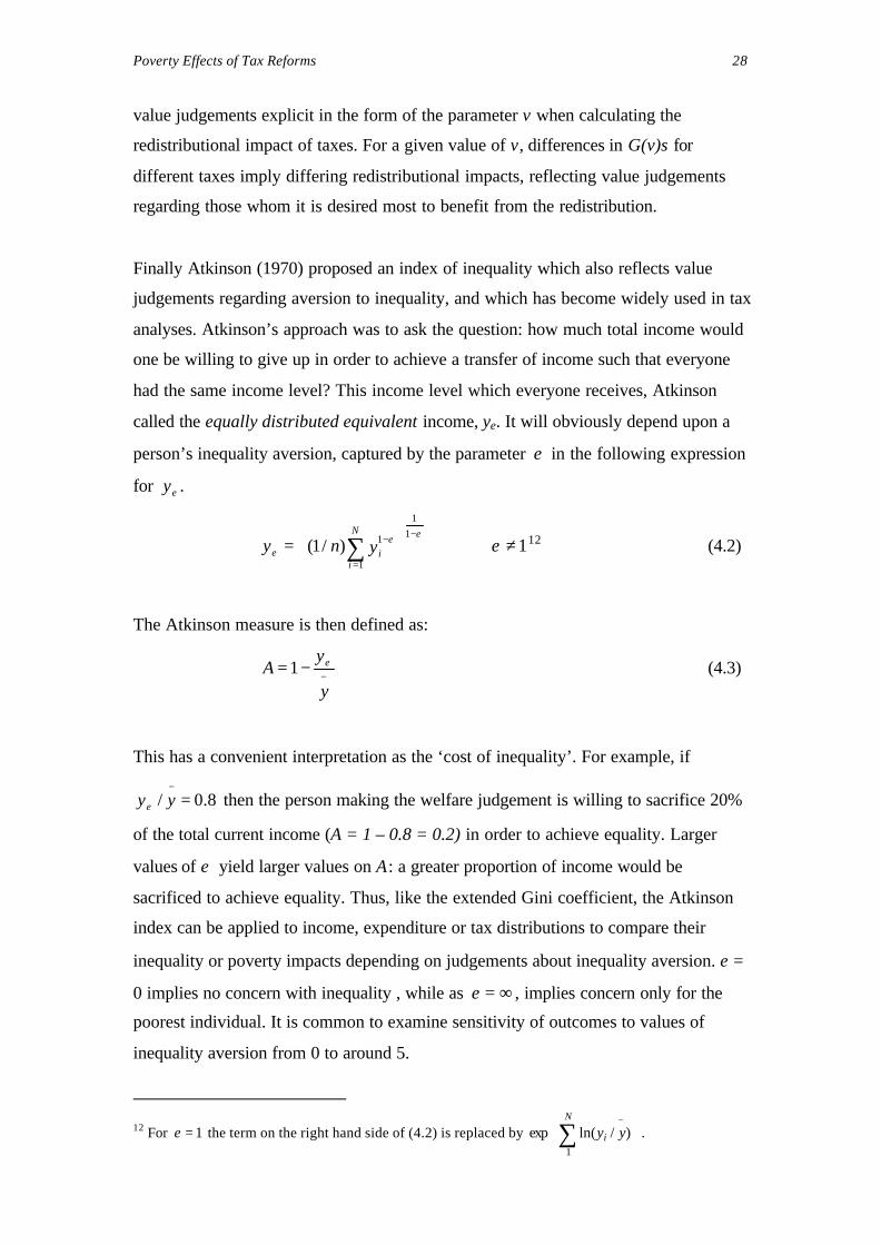
Poverty Effects of Tax Reforms 28
value judgements explicit in the form of the parameter v when calculating the
redistributional impact of taxes. For a given value of v, differences in G(v)s for
different taxes imply differing redistributional impacts, reflecting value judgements
regarding those whom it is desired most to benefit from the redistribution.
Finally Atkinson (1970) proposed an index of inequality which also reflects value
judgements regarding aversion to inequality, and which has become widely used in tax
analyses. Atkinson’s approach was to ask the question: how much total income would
one be willing to give up in order to achieve a transfer of income such that everyone
had the same income level? This income level which everyone receives, Atkinson
called the equally distributed equivalent income, ye. It will obviously depend upon a
person’s inequality aversion, captured by the parameter ε in the following expression
for ey .
εε −
=
−
= ∑1
1
1
1)/1(N
iie yny 1≠ε 12 (4.2)
The Atkinson measure is then defined as:
−−=
y
yA e1 (4.3)
This has a convenient interpretation as the ‘cost of inequality’. For example, if
8.0/ =−yye then the person making the welfare judgement is willing to sacrifice 20%
of the total current income (A = 1 – 0.8 = 0.2) in order to achieve equality. Larger
values of ε yield larger values on A: a greater proportion of income would be
sacrificed to achieve equality. Thus, like the extended Gini coefficient, the Atkinson
index can be applied to income, expenditure or tax distributions to compare their
inequality or poverty impacts depending on judgements about inequality aversion. ε =
0 implies no concern with inequality , while as ∞=ε , implies concern only for the
poorest individual. It is common to examine sensitivity of outcomes to values of
inequality aversion from 0 to around 5.
12 For 1=ε the term on the right hand side of (4.2) is replaced by
∑
−N
i yy1
)/ln(exp .

Poverty Effects of Tax Reforms 29
Poverty Measures
Presuming readers are familiar with the main poverty measures this section will
discuss these only briefly. Measuring the impact of different taxes on poverty has been
much less prevalent than assessing inequality impacts. Studies that have been
undertaken demonstrate the importance of the particular poverty measure chosen for
conclusions reached. The most commonly used measures in tax analyses are:
head count (the numbers, or proportion, below a specified poverty line);
poverty gap (the average income of those in poverty relative to the poverty line); and
‘inequality of poverty’ (the dispersion of incomes within the poor group).
Foster et al (1984) show that these measures fall within the general class of poverty
measures captured by:
∑≤
−=
pi yy p
i
yy
NP
θ
θ 11
(4.4)
where θ is an integer parameter, and yp is the poverty level. P0 is the head count
measure – the proportion of the population in poverty, NP/N; P1 depends on P0 and the
poverty gap; and P2 includes inequality within the poor. Jenkins and Lambert (1997)
have referred to these as the ‘Three “I”s of Poverty’: incidence, intensity and
inequality, and proposed a ‘TIP curve’ to capture these three aspects. TIP curves, like
Lorenz curves, can be constructed for any income/expenditure measure and plot the
total poverty gap per capita against the cumulative proportion of the population below
that gap (from lowest to highest). See Creedy (1998a) for further details.
An example is shown in Figure 4.1. The horizontal axis measures P0, the vertical axis
measures the poverty gap; while the concavity of the TIP curve below the poverty line
measures inequality within the poor. Beyond the poverty line, (set at 10 units, giving
P0 = 0.4, in Figure 4.1) the TIP curve becomes horizontal. If the TIP curve for one
distribution lies closer to the horizontal axis than another, then the former involves less
poverty as measured by the poverty gap. If only the head count measure of poverty is
considered as relevant, proximity of a TIP curve to the vertical axis is preferred.13
Though TIP curve comparisons could provide valuable information on the poverty
13 Normalised TIP curves can also be obtained (by dividing the poverty gap by the poverty line) - so thatthe values on both axes lie between 0 and 1. This allows poverty dominance tests to be conducted of thesort described above for inequality using Lorenz curves.

Poverty Effects of Tax Reforms 30
impacts of different taxes, we are not aware of any examples applied to developing
countries. Creedy (1998a) uses them to examine hypothetical tax and transfer schemes.
Measures of Social Welfare
Is one tax preferred to another? Perhaps the most common approach by economists to
answer that question is to construct a measure of social welfare (from some
combination of the well-being of individuals or households) and examine the impact of
the taxes in question on that measure. For the case of indirect taxes, the most relevant
case for most LDCs, the standard approach is to construct money-metric measures of
utility – usually income – and consider how a given indirect tax, which changes goods
prices, affects this utility measure. Individual utilities, or utility changes, are then
aggregated according to the social welfare function, which specifies how different
individuals are weighted.
The most common measure of welfare change of this sort is the Equivalent Variation
(EV). Consider an increase in the prices of goods resulting from the imposition of a set
of taxes. Compared to a no-tax situation this will make an individual feel less well off
(reduce welfare).The EV is the amount of money which this individual would be
willing to pay to avert the change in prices.14 EVs therefore provide a money measure
of the welfare losses suffered as a result of the tax change. They can be calculated for
specified groups or types of individuals (or households), or aggregated to measure
overall welfare losses. Aggregation however requires specific judgements about
household weightings, so most studies using EVs report them for specified, relatively
homogeneous, groups.15
A simple way of measuring effects on social welfare is the Abbreviated Social
Welfare Function. Lambert (1993) shows how welfare rationales can be used to
justify the abbreviated forms:
)](1[ vGW −= µ and )](1[ εµ AW −= (4.5)
14 A similar alternative measure is the Compensating Variation – see Creedy (1998b) for details.15 An alternative welfare measure, the Excess Burden (EB) of taxation, subtracts the value of the taxrevenue raised from the EV in order to identify the net welfare gain or loss for each individual. Moststudies of LDCs ignore this revenue component because of the difficulties identifying the amount of taxrevenue paid by each individual. Where additional tax revenues are squandered (in the sense that theyproduce no, or few, social benefits) it would be more appropriate to use the EV in any case.

Poverty Effects of Tax Reforms 31
where G(v) and )(εA are the extended Gini and Atkinson inequality indices discussed
above. (4.5) shows that welfare can be measured simply as the mean income multiplied
by an index of equality (one minus the inequality index). Since IFI reforms might be
expected to affect mean income, the abbreviated SWF provides a useful tool to assess
the equity-efficiency trade-offs using the Gini or Atkinson measures. By adopting
different values for the inequality aversion parameters, ),( εv , (4.5) can focus on
poverty effects rather than more general inequality effects. The major difficulties of
this approach in practice are likely to be separating the effects of tax changes from
other influences on mean incomes and equity.
The concept of the Marginal Social Cost (MSC) of taxes was developed and extended
to the context of LDC tax reform in the 1980s and ‘90s (see Ahmed and Stern, 1984,
1991; Stern, 1987).16 This approach is applied to marginal tax changes, where the
question being asked is: would a marginal increase in tax i, funded by a marginal
decrease in tax j improve welfare? If desired welfare can be specified to focus
exclusively on those in poverty.
The MSC of a tax can be defined as:
)/)(/(//
RttWtRtW
iii
ii ∂∂∂∂=
∂∂∂∂
=λ (4.6)
where W∂ and R∂ are respectively the change in welfare and tax revenue. Thus, (4.6)
can be interpreted as the change in welfare, W, brought about by the change in tax rate,
ti which is required to raise one additional unit of revenue, R. If λi is greater than the
equivalent for an alternative tax, λj, then the social costs associated with tax i are
greater than those for tax j. Reform could beneficially reduce the tax rate on i and
increase it on j. Clearly reforms that raise welfare and do not lower total tax revenues
are preferred in this framework. However, welfare-raising reforms which reduce
revenue cannot be unambiguously evaluated without knowledge or assumptions about
the use of the foregone revenues. The MSCs can readily be calculated from information
on consumers’ expenditures, tax rates, aggregate cross-price elasticities, and welfare
weights chosen by the investigator (see Creedy, 1998a; Madden, 1995, 1996).
16 The wider literature on this concept is reviewed by Creedy (1998b). The MSC concept is closelyrelated to the concept of the Marginal Costs of Funds (MCF). The latter concept is the relevant measurewhen considering the welfare costs of raising tax revenues to fund additional expenditures, while the

Poverty Effects of Tax Reforms 32
Evaluating marginal reforms is therefore much less data intensive than evaluations of
non-marginal reforms. What constitutes ‘marginal’ in this context is open to some
interpretation. If general equilibrium effects are not thought to be large, the MSC
approach may provide a reasonable approximation even for relatively large shifts in tax
structure. Where there are substantial changes in the tax system, and behavioural
responses are thought likely to be important, Computable General Equilibrium
(CGE) models are usually the preferred method of analysis. These model social
welfare and economic behaviour across the economy explicitly, typically assuming
price flexibility and using the equivalent variation to measure the social welfare effects
of tax changes (see chapters 5 and 6).
4.4 The Inflation Tax
Tax reforms that reduce revenues, without any commensurate reduction in
expenditures, must be funded from some other source. For governments in LDCs
struggling to find sufficient funding, money creation can be a convenient alternative
with familiar consequences for inflation. The resulting ‘inflation tax’ is just as much a
tax as any other and can therefore have analogous distributional consequences.17
Revenue from the inflation tax may be defined as:
mR ππ = (4.7)
where π is the inflation rate and m is real money balances (the tax base). Dividing both
sides by real income, y, gives the ‘average inflation tax rate’:
)/(/ ymyRATR πππ == (4.8)
One way of assessing the distributional impact of the inflation tax would be to examine
its average rate progression. From (4.8), this will depend on (i) how the inflation rate
faced by individuals differs by income levels; and (ii) how the money balances-to-
income ratio differs with income levels. In the case of (i), to the extent that
consumption bundles differ between the poor and the rich, and inflation rates are not
uniform across all goods, there is the potential for differing incidence of the inflation
tax. A pertinent issue here concerns the case where goods consumed predominantly by
the poor are subsidised. It can be shown that if the producer prices of all goods inflate
at the same rate, the consumer prices of subsidised goods will inflate at a higher rate
MSC is the relevant measure when comparing alternative, revenue-neutral taxes. In fact the twomeasures are related by: MSC = MCF – 1.17 This argument is just as relevant for revenue-enhancing tax reforms since the additional tax revenuesmay facilitate reduced reliance on the inflation tax.

Poverty Effects of Tax Reforms 33
(unless the subsidy is increased at the inflation rate). In this case consumers of
subsidised goods face a higher effective inflation tax rate.
With respect to (ii) above, the variation in the m/y ratio across income levels is unclear
a priori. The poor who operate largely outside the monetary economy will be
essentially unaffected. However, for those who do participate in the monetary
economy, the poor may have more of their assets in the form of cash and may have a
more limited capacity to raise nominal incomes in order to maintain real incomes in an
inflationary environment. On the other hand the poor hold few financial assets subject
to erosion by inflation so that they may gain relative to richer households in this
respect. We know of no direct evidence on the cross-sectional variation in money-
income ratios which would shed light on this issue. However, a recent assessment by
Adam and Bevan (2001) concludes that ‘there is a strong consensus that higher
inflation is at least as costly to the poor as it is to other sections of the population,
reflecting mainly the lesser ability of the poor to protect their factor incomes and asset
portfolios from the effects of inflation. At the least, there is nothing to suggest that
targeting a low rate of inflation … would be contra-indicated when the interests of the
poor are taken into account’.
Creedy (1998b) examined the distributional effects of inflation in Australia and New
Zealand in the 1990s and found (i) distributional effects were small (inequality indices
increased by less than 1%); (ii) effects were mildly regressive in most years but were
progressive in some; and (iii) inequality effects were greatest in years of highest
inflation. This last effect suggests the possibility of larger effects in those LDCs which
suffer from higher rates of inflation over prolonged periods. However, even if the
inflation tax is generally proportional, reform assessments must recognise that, with
lower inflation, revenue-neutrality may require increased reliance on an alternative
regressive or progressive tax.
4.5 Issues Arising for Applications in LDCs
The discussion in sections 4.2 and 4.3 suggests a number of issues to be addressed
when tax incidence is examined in an LDC context.
Poverty Effects of Tax Reforms 34
The inappropriateness of traditional tax incidence assumptions for many LDC
applications has been highlighted by Shah and Whalley (1991). They argued that
quantitative restrictions on many imports, general price controls and regulations, the
existence of informal (and other non-taxable) markets, rural-urban migration and tax
evasion affect the ability of those legally liable for various taxes to shift these as
traditionally assumed. Table 4.2 below summarises their main arguments. CGE
modelling (see chapter 5) suggests that altering incidence assumption can lead to quite
different conclusions regarding who bears the burden of taxes in LDCs. Empirical
applications of other methods have made limited changes to incidence assumptions,
but some recognition of the issues represented in Table 4.2 could be attempted.
Assessing the incidence of import taxes is further complicated by the fact that
consumption expenditure data does not normally distinguish imports from domestic
goods. Recently Rajemison and Younger (2001) have proposed using input-output
tables to help resolve this issue. For most indirect taxes, however, it is always likely to
be the case that incidence will remain uncertain, supporting the case for sensitivity
analyses.
Tax evasion is an especially serious issue that affects incidence and is difficult to
include. Existing incidence studies, which ignore evasion, can be thought of as
providing a benchmark of what ‘full implementation’ of the tax would produce. In
some cases, access to actual tax revenues can reveal the extent to which receipts fall
short of expectations based on statutory rates and this could be used to gauge
‘compliance rates’. Jenkins and Kuo (2000) discuss possible uses of compliance ratios
in a VAT simulation model, though they focus on revenue, rather than redistributional,
aspects.
Taxation of intermediate inputs is significant in some LDCs. In such cases it is
important that incidence analyses are based on effective, not nominal, tax rates.
Younger (1996) and Younger et al (1999) argue, for Ghana and Madagascar, that
taxation of petroleum is an important example. Since fuel is sold as an intermediate as
well as a final good, fuel taxation can affect other final goods such as transport,
consumed by the poor. In the absence of input-output data, they make an informed

Poverty Effects of Tax Reforms 35
guess regarding the pass-through of fuel taxes to transport.18 Ahmed and Stern (1987,
1991) however calculated effective commodity tax rates for India and Pakistan and
showed that goods consumed disproportionately by the poor can face positive effective
rates even though nominal rates were zero or negative (subsidy). Nominal-effective
differences were widespread. Education, for example, was essentially untaxed
(nominally) but faced an effective tax rate of around 9%. Some examples are given in
Table 4.3 below.
4.6 Conclusions
A number of conclusions emerge, even at this stage, for studies of the poverty impacts
of taxes and tax reforms.
1. Given uncertainties over incidence, evasion etc., different methods should be
compared wherever possible.
2. Within a given method, sensitivity testing of assumptions should be pursued as
far as possible.
3. Data constraints in individual country settings are likely to influence strongly the
type of analysis that can be undertaken. Where data are more severely limited,
the ARP approach can provide useful information (especially if alternative
incidence assumptions can be applied) but must be interpreted with care.
However, many countries now have some form of household expenditure survey
data which can be used to improve the ARP approach and allow the construction
of tax concentration curves, dominance testing and the use of fiscal simulation
models.
4. The counterfactual against which the tax in question is being compared must be
considered carefully. The usual counterfactual is a proportional tax yielding the
same revenue. However, tax comparisons in practice in LDCs (e.g. pre- and post-
reform), may involve increased or reduced revenues so that observed poverty or
inequality changes cannot be unambiguously attributed solely to the tax change
but may represent the effects of growth. There are two options here. Firstly,
comparisons can be made whereby both taxes generate equal revenues. Secondly
if revenues change after reform, consideration can be given to how this revenue
(including deficit finance) would likely have been raised in the absence of
reform. The new tax should then be compared with this alternative.
18 Rajemison and Younger (2001) use I-O tables to allow for this effect more carefully.

Poverty Effects of Tax Reforms 36
5. It is often wrong to think that sectors or individuals that are not taxed directly
therefore bear no tax incidence. In addition to the effect of the taxation of
intermediates, informal sectors and poor consumers may find the prices of their
product affected by taxation elsewhere. Though no tax revenue arises from this,
untaxed sectors certainly bear some of the tax incidence, and (typically poor)
consumers and producers of informal sector products can both be affected. The
inflation tax is a clear example of a tax which the poor do pay and where this tax
is used to avoid raising conventional taxes for which the poor are not liable, the
inflation tax effectively transfers tax burdens to the poor.
Table 4.1 Tax Incidence Assumptions
Tax Statutory
incidence
Traditional economic
incidence
Personal income tax: income recipients income recipients (i.e. no shifting)
Corporate taxes: firms shifted backwards to capital owners
or forwards to consumers of taxed
products
Domestic indirect taxes
(e.g. sales taxes, excises):
Producer, retailer,
manufacturer, etc
shifted forwards to consumers
Trade taxes: imports importers shifted forwards to consumers
exports exporters exporters
Payroll taxes:
employer contrib. employer employer or shifted to employee
employee contrib. employee employee
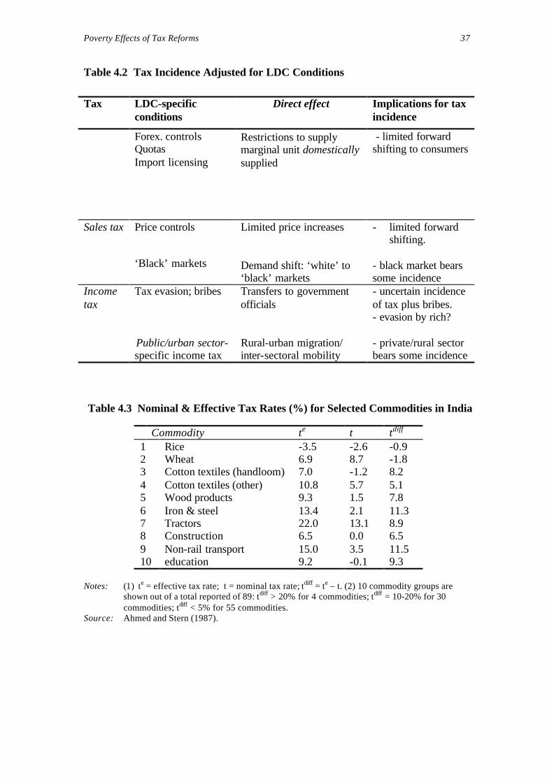
Poverty Effects of Tax Reforms 37
Table 4.2 Tax Incidence Adjusted for LDC Conditions
Tax LDC-specificconditions
Direct effect Implications for taxincidence
Forex. controlsQuotasImport licensing
Restrictions to supply ⇒marginal unit domesticallysupplied
- limited forwardshifting to consumers
Sales tax Price controls
‘Black’ markets
Limited price increases
Demand shift: ‘white’ to‘black’ markets
- limited forwardshifting.
- black market bearssome incidence
Incometax
Tax evasion; bribes
Public/urban sector-specific income tax
Transfers to governmentofficials
Rural-urban migration/inter-sectoral mobility
- uncertain incidenceof tax plus bribes.- evasion by rich?
- private/rural sectorbears some incidence
Table 4.3 Nominal & Effective Tax Rates (%) for Selected Commodities in India
Commodity te t tdiff
1 Rice -3.5 -2.6 -0.92 Wheat 6.9 8.7 -1.83 Cotton textiles (handloom) 7.0 -1.2 8.24 Cotton textiles (other) 10.8 5.7 5.15 Wood products 9.3 1.5 7.86 Iron & steel 13.4 2.1 11.37 Tractors 22.0 13.1 8.98 Construction 6.5 0.0 6.59 Non-rail transport 15.0 3.5 11.510 education 9.2 -0.1 9.3
Notes: (1) te = effective tax rate; t = nominal tax rate; tdiff = te – t. (2) 10 commodity groups areshown out of a total reported of 89: tdiff > 20% for 4 commodities; tdiff = 10-20% for 30commodities; tdiff < 5% for 55 commodities.
Source: Ahmed and Stern (1987).

Poverty Effects of Tax Reforms 38
Figure 4.1 TIP Curves
Data for TIP curves in Figure 4.1Incomes of individuals
1 2 3 4 5 6 7 8 9 10Distn 1 4 6 8 9 12 15 20 25 30 35Distn 2 4 6 11 11 12 15 20 25 30 35Distn 3 7 8 8 9 12 15 20 25 30 35Distn 4 6 7 8 11 12 15 20 25 30 35
0
0.2
0.4
0.6
0.8
1
1.2
1.4
0 0.1 0.2 0.3 0.4 0.5
proportion of population, Po
tota
l po
vert
y g
ap p
er c
apit
a, P
1
TIP 1
TIP 2
TIP 3
TIP 4

Poverty Effects of Tax Reforms 39
Chapter 5 Evidence on the Distributional Impact of Taxes and Tax Reform
This chapter reviews the evidence from different approaches on the distributional
effects of taxes and tax reforms. The most popular, traditional, approach was the
Average Rate of Progression (ARP) measure (section 5.1). Evidence is now also
available for several countries using concentration curve and welfare dominance
concepts (section 5.2). These measures have generally been used to asses the
progressivity of existing taxes rather than compare pre- and post-reform regimes (an
exception is Chen et al (2001) for Uganda) but they can nevertheless shed light on this
issue. Marginal social cost evidence (section 5.3) addresses reform explicitly, both
actual and counterfactual. Finally, evidence from CGE and fiscal simulation
approaches are examined in sections 5.4 and 5.5 respectively.
5.1 Tax Progression EvidenceNumerous studies, calculating average tax rates by income level or across income
groups were undertaken during the 1960s and ‘70s. They used statutory tax rates and
traditional shifting assumptions and are of questionable reliability, especially early
studies where data were particularly limited. Jimenez (1986) and Gemmell (1987)
review this evidence. Although the terms ‘progressivity’ and ‘regressivity’ are
regularly used in these studies, the evidence relates simply to departures from
proportionality of the taxes concerned. Broadly, the evidence is as follows:
Personal income taxes progressive (but evasion generally ignored)
Corporate taxes U-shaped (regressive then progressive)
Property Taxes progressive? (but generally low revenue share)
Indirect taxes regressive
Overall tax system varied, often regressive at low incomes
Jimenez (1986) reports overall tax incidence from various country studies (Table 5.1).
In cases where progressivity is found, this is often because income tax evidence
dominates (but where the use of statutory tax rates and thresholds is especially
unreliable). Despite this, the combined effect of taxes in many countries appear to be
regressive at lower income levels, even if they appear to be progressive further up the
income scale. One problem with this evidence for indirect taxes (import taxes, sales
taxes etc) is that progression has often been measured with respect to income levels

Poverty Effects of Tax Reforms 40
rather than expenditures. As discussed in chapter 4, this can lead to apparent evidence of
regressive indirect taxes when, in fact, it reflects the income-expenditure relationship.
5.2 Progressivity Evidence: Concentration Curves and Inequality Measures
Recent work by Stephen Younger and colleagues has begun to report concentration
curves (with associated welfare dominance tests) and Gini coefficients for several taxes
in African countries (see Younger, 1996; Sahn and Younger, 1998; Younger et al,
1999; Rajemison and Younger, 2001; Chen et al, 2001). These are generally based on
statutory tax rates and traditional incidence assumptions, but do allow for some shifting
of intermediate goods taxes. Rajemison and Younger use input-output tables to track
incidence across goods/sectors, and calculate tax rates from actual collections, for
indirect taxes in Madagascar.
Evidence on tax progressivity/regressivity from dominance testing is shown in Table
5.2 for six African countries: Cote d’Ivoire, Ghana, Guinea, Madagascar, Tanzania and
Uganda. Taxes are designated as progressive (regressive) if the concentration curve for
the relevant tax lies wholly outside (inside) that for household expenditures and the
difference is statistically significant. Where this cannot be established, the tax is shown
as ‘neutral/inconclusive’.
When considering beneficial reforms the ‘welfare dominate’ criterion is useful, as
dominance implies a preference for the dominating tax regardless of the weight given
to the poorest. Tables 5.3 – 5.6 report results for Cote d’Ivoire, Guinea, Madagascar
and Tanzania (similar results are not available for Ghana). In each table the taxes in the
left-hand column are arranged in descending order of progressivity; for example, in
Guinea (Table 5.4), gasoline and diesel taxes are estimated as most progressive,
followed by taxes on beverages, alcohol, automobiles, etc. The right-hand column
shows those taxes that are welfare dominated by the associated tax in the left-hand
column. What emerges from this evidence is:
• Taxes on private transport (gasoline, autos) tend to be strongly preferred on
distributional grounds.
• VAT and sales taxes are more progressive than import taxes or excises, though
usually not by enough for statistical tests to confirm welfare dominance.

Poverty Effects of Tax Reforms 41
• Export taxes and taxes on kerosene are often regressive and are strongly dis-
preferred to any other taxes.
• Progressivity of the so-called ‘sin taxes’ on alcohol and tobacco is variable. In 3 of
the 4 countries alcohol taxes are more progressive than tobacco taxes, but only in
Cote d’Ivoire is tobacco taxation regressive.19
• Uniform taxation of fuel would be problematic because of the very different
consumption patterns for gasoline and kerosene (or paraffin), which are
respectively highly pro-rich and pro-poor in their consumption.
Rajemison and Younger (2001) investigate incidence using (i) actual tax payments to
calculate tax rates; and (ii) input-output (I-O) tables to calculate effective tax rates, in
Madagascar where intermediates form over 60% of imports and 80% of petroleum
consumption. They find that (i) substantially reduces tax rates while (ii) significantly
increases them. Two examples are given below:
VAT Import Duty
Industry statutory actual I-O based statutory actual I-O based
Tobacco 7.7 0.6 3.6 7.8 0.2 1.6
Textiles 11.4 1.2 3.5 17.6 0.7 2.1
However, all three methods (including using statutory rates) produce similar progressivity
rankings except for the two taxes where intermediate use is important: import duties and
petroleum tax. However, it is the use of actual tax rates, rather than allowing for I-O
effects, which has a substantial effect on progressivity results.
For import duties, conventional incidence assumptions produced a regressive outcome
whereas they were progressive (and could not be dominated by any other taxes ) using I-
O methods. Traditional incidence assumptions for tariffs may, therefore, be seriously
misleading; an important observation for evaluation of IFI-type reforms. One
methodological difficulty with the I-O approach however is that it can require
considerable aggregation across goods in order to estimate effective tax rates, reducing
the accuracy of progressivity comparisons. In the case of Madagascar, applying I-O
methods reduced the number of goods examined from 222 to 30!
19 Tobacco taxes also appear to be regressive in Ghana except at high income levels.
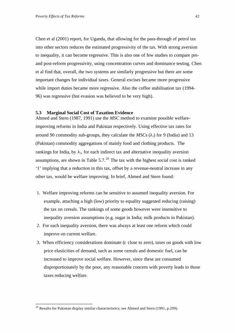
Poverty Effects of Tax Reforms 42
Chen et al (2001) report, for Uganda, that allowing for the pass-through of petrol tax
into other sectors reduces the estimated progressivity of the tax. With strong aversion
to inequality, it can become regressive. This is also one of few studies to compare pre-
and post-reform progressivity, using concentration curves and dominance testing. Chen
et al find that, overall, the two systems are similarly progressive but there are some
important changes for individual taxes. General excises became more progressive
while import duties became more regressive. Also the coffee stabilisation tax (1994-
96) was regressive (but evasion was believed to be very high).
5.3 Marginal Social Cost of Taxation EvidenceAhmed and Stern (1987, 1991) use the MSC method to examine possible welfare-
improving reforms in India and Pakistan respectively. Using effective tax rates for
around 90 commodity sub-groups, they calculate the MSCs (λi) for 9 (India) and 13
(Pakistan) commodity aggregations of mainly food and clothing products. The
rankings for India, by λi, for each indirect tax and alternative inequality aversion
assumptions, are shown in Table 5.7.20 The tax with the highest social cost is ranked
‘1’ implying that a reduction in this tax, offset by a revenue-neutral increase in any
other tax, would be welfare improving. In brief, Ahmed and Stern found:
1. Welfare improving reforms can be sensitive to assumed inequality aversion. For
example, attaching a high (low) priority to equality suggested reducing (raising)
the tax on cereals. The rankings of some goods however were insensitive to
inequality aversion assumptions (e.g. sugar in India; milk products in Pakistan).
2. For each inequality aversion, there was always at least one reform which could
improve on current welfare.
3. When efficiency considerations dominate (ε close to zero), taxes on goods with low
price elasticities of demand, such as some cereals and domestic fuel, can be
increased to improve social welfare. However, since these are consumed
disproportionately by the poor, any reasonable concern with poverty leads to those
taxes reducing welfare.
20 Results for Pakistan display similar characteristics; see Ahmed and Stern (1991, p.209).

Poverty Effects of Tax Reforms 43
5.4 CGE EvidenceBecause of their multi-sector nature, CGE models are best suited to examining the
implications of changing incidence assumptions and evaluating major tax restructuring.
A number of CGEs have now been constructed for individual LDCs to explore the
distributional impact of taxes. For example, Clarete (1991) and Shah and Whalley
(1991) examine the progressivity of various taxes in the Philippines and Pakistan
respectively, the latter distinguishing between urban and rural income earners. Dahl
and Mitra (1991) apply CGE tax models to Bangladesh, China and India and explore
distributional effects by industrial sector, between formal and informal, and between
rural and urban areas.
For Pakistan, Shah and Whalley found that the effect of changing incidence
assumptions (presumed to reflect the institutional and economic conditions in LDCs
better) led to very different conclusions regarding progressivity. Table 4.2 in chapter 4
summarised the main difference in incidence assumptions proposed by Shah and
Whalley. In essence the arguments are two-fold.
1. Quantitative restrictions can mean that indirect taxes are not fully passed on to
consumers in prices. Instead, some or all of the incidence is borne by the importer or
domestic producer. (Quantitative restrictions include import quotas or licenses, direct
price controls or restrictions which limit price flexibility, or foreign exchange).
2. Income taxes are generally restricted to modern, urban or public sectors. This
renders these sectors less attractive to potential employees, or limits the supply of
jobs. The consequence is increased supply of labour to other (e.g. rural) sectors
which depresses wages there. Some incidence of the tax is therefore borne by
untaxed sector producers or workers or both.
The second effect is probably not quantitatively important in most countries (because
income taxes are little used), but may be relevant in specific cases. The first effect,
however, could be substantive enough to raise doubts about the distributional
conclusions reached by existing studies using conventional incidence assumptions.
Shah and Whalley (1991) provide some evidence on this but only for trade taxes. They
show that, in Pakistan, traditional assumptions would lead to a regressive conclusion.
They argue however, that quantitative restrictions would cause some of the incidence
to fall on import and export license holders; and assume that the incidence rests with
capital income earners. The link here is a tenuous one and Shah and Whalley

Poverty Effects of Tax Reforms 44
experiment with alternative assumptions regarding which capital income earners are
affected. These alternatives lead to trade taxes appearing to be progressive, sometimes
strongly so.
It remains unclear how far these arguments apply to domestic indirect taxes. The key
issue is whether supply curves for taxed goods can reasonably be thought of as
perfectly elastic at the margin. If not, there is good reason to think that not all of the
incidence of indirect taxes will fall on consumers of those products. In addition it
should be remembered that Shaw and Whalley provide no data in support of their
alternative incidence assumptions.
Clarete (1991) undertakes a similar exercise for major Philippine taxes (allowing for
imports and foreign exchange restrictions and rural-urban migration). He shows that,
allowing for these three institutional effects (one at a time), leads to different
conclusions for excise taxes, VAT and tariffs. Corporate and personal income tax
results are essentially unchanged.21 The importance of incidence assumptions for
model results is confirmed by Chia et al’s (2000) CGE model of Ivorian tax incidence.
Two other key results emerge from this study. (i) Incidence may vary considerably
across socio-economic groups which does not translate into a simple income ranking –
the poor in one sector may suffer while the poor elsewhere gain. (ii) Allowing for
inter-household transfers (e.g. remittances from urban to rural households)
substantively affects incidence results.22
Coady and Harris (2001) used CGE methods to measure the social cost of raising
revenues from alternative VAT systems (single- and multi-rate, exemptions etc) to
finance transfers to the poor in Mexico. They show that with even modest concern for
the poor (inequality aversion) there are social gains from all VAT options but all are
dominated by financing the transfers by reducing food subsidies. They also show that
if concern is with the very poorest, raising tax revenues to finance transfers can be
21 Further examples of CGE simulations of the distributional impact of taxes under different assumptionscan be found in Choon (2000), Chia et al (2000), and Lora and Herrera (2000), for Singapore, Coted’Ivoire, and Colombia respectively.22 This is a case where it is important to analyse tax and expenditure incidence together. If,hypothetically, inter-household transfers were instead paid to the government in tax and the governmentmade equal transfers to those households, tax incidence would change considerably but no differencemay have occurred in households income positions. The incidence of the transfers should be examinedalongside that for taxes.

Poverty Effects of Tax Reforms 45
socially costly in the sense that, although tax incidence is low for the poor in general it
can be higher on the very poorest (with any incidence on the poorest being treated as
especially costly).
In summary, much CGE evidence must be regarded as ‘suggestive’ rather than
conclusive, but three tentative conclusions are:
• there is greater uncertainty concerning the distributional effects of taxes in LDCs
than had generally been appreciated;
• overall the tax system may be more progressive than is often presumed;
• sector-specific taxes, and segmented LDC markets, can lead to incidence effects
differing as much across sectoral or socio-economic groups as across income levels.
Shah and Whalley’s own summary of the impact of adopting their alternative tax
shifting assumptions (in Table 4.2) is:
Tax: Traditional incidence
assumptions
‘New’ assumptions
reflecting LDC conditions
Income tax Progressive Ambiguous
Corporate tax Progressive/Proportional Progressive
Sales/VAT taxes Regressive Progressive
Trade taxes Regressive Progressive
Payroll taxes Ambiguous Ambiguous/Progressive
Urban property tax Regressive/Progressive Progressive
Finally, Ahmed and Stern (1987, 1991) have explored the distributional impact of
(hypothetical) major reforms in India and Pakistan, involving the replacement of some
or all of the existing excise taxes with a proportional VAT. Estimating Equivalent
Variations separately for 14 urban and 14 rural income groups, they show that a
revenue-neutral reform could reduce poor rural households expenditures by as much
almost 7% (and 5% for poor urban households). The richest households gain by up to
4%. Even exempting cereals from the VAT (to assist the poor), still produces welfare
losses for the poorest 6 rural (10 urban) groups. This suggests a trade-off between
improvements in efficiency and poverty. However, reform involving domestic sales

Poverty Effects of Tax Reforms 46
taxes can be tailored to help the poor but probably only at the cost of increasing the
complexity of the system (e.g. with exempt goods and more than one tax rate). As
Ahmed and Stern (1987, p.320) note, for India: ‘it would be interesting … to study a
system with, for example, a selective VAT, plus food subsidies, plus special taxation of
selected items such as gasoline and some luxury items. We could very probably
produce a package that would lose no revenue and would look attractive in terms of
the above [welfare] analysis’.
5.5 Evidence from Fiscal Simulation Models
Fiscal simulation models use simple simulation techniques to capture the essential
features of income and expenditure distributions, and combine these with tax structure
information to examine revenue, redistributional and welfare effects of tax systems and
reform. Where information is available, or plausible assumptions can be made, they
can be extended to incorporate consumers’ and labour supply responses. In this case
they resemble more narrowly focused CGE models. The most sophisticated fiscal
simulation models have been produced for developed countries (e.g. by the IFS for the
UK; Creedy (1999) for Australia and New Zealand). Where there is limited modelling
of behaviour, these models are best suited to examining the ‘impact’ (i.e. short-run)
effects of tax reforms.
So far, applications to LDCs have been limited to simulating revenue aspects using
fairly simple models (see Jenkins and Kuo, 2000). More sophisticated models have
been applied to Australia, New Zealand and the UK by Creedy (1998, 1999) and
Creedy and Gemmell (2001a, b). This evidence is not relevant here but there is
potential to adapt these models for LDCs (see chapter 6). Jenkins and Kuo (2000) use
data on incomes and expenditures across income groups in Nepal to consider the
revenue effects of replacing an existing sales tax and set of excises with a VAT. This
type of analysis can focus on details of the tax system, can simulate different degrees
of tax compliance (using actual tax collection evidence as a guide), and can consider
the effects of base broadening, alternative tax rates etc. For Nepal, Jenkins and Kuo use
the model to estimate the VAT rate which would be required to yield equal or greater
revenues to these produced by the current system, examining this for alternative
compliance rates.

Poverty Effects of Tax Reforms 47
5.6 The Revenue Effects of Tax Reform
A major concern with reforms to trade regimes in LDCs has been whether tax revenues
would be depleted or enhanced by the changes to tariffs etc. Evaluating long term
effects is made difficult by the fact that numerous other changes take place in an
economy in the years following reform. As a result most revenue assessments look at
relatively short-term or ‘impact’ effects. Over the longer term, Adam and Bevan (2001,
pp.12-13) argue that most LDCs need a tax structure yielding revenues around 15-20%
of GDP to fund public expenditures around 20% of GDP. They also note that similar
post-reform tax structures across countries are associated with very different tax/GDP
ratios suggesting that differences in compliance and administrative efficiency may be
important. Indeed, some of the best examples of successful stabilisation programmes
(e.g. Uganda, Tanzania) have been associated with tax/GDP ratios around 11-12%.
This is likely to lead to severe funding problems over the longer term unless reformed
tax systems can generate additional revenues or donor agencies are willing to make up
the shortfall. The latter seems unlikely in most cases.
Two reviews of the short-run (up to 5 years) revenue effects of trade reform
(Greenaway and Milner, 1991; Devarajan and Panagariya, 2000) find examples of both
revenue-enhancement and depletion, but with the former appearing to dominate. Their
particular focus is on trade tax reforms which restructure the import and export
tax/quota systems (elimination or reduction in export taxes; reductions in tariff rates;
‘tariffication’ of import quotas). There is no clear a priori prediction but Greenaway
and Milner find 3 out of 5 countries undertaking SAL programmes experienced trade
revenue increases (as a % of GDP); the other two experience revenue reductions.
Devarajan and Panagariya (2000) examined 40 trade reform episodes in 22 developing
countries, and found that in 25 of those trade or import tax revenues rose, 2 showed no
change and 15 experienced trade/import revenue declines. These results are
encouraging both because of the majority of enhancement cases and because
arguments for broader fiscal reform have often presumed that new revenue sources
would be needed to counteract trade tax revenue loses. If post-reform trade tax
revenues can be maintained or increased, it is more likely that reforms to domestic
taxes can complement this and assist in further revenue raising.
Poverty Effects of Tax Reforms 48
5.7 ConclusionsWhat conclusions can be drawn from the above evidence? Firstly, general conclusions
with respect to particular taxes are quite hard to find – progressivity/regressivity
conclusions are often country specific. To the extent that the incidence of indirect taxes
rests with consumers (i.e. prices adjust by the full amount of the tax), evidence from
ARP studies, concentration curves and welfare dominance tests point to taxes on
exports (cocoa in Ghana; coffee in Uganda; vanilla in Madagascar), intermediates,
and kerosene excises as bad for the poor. In general, one would also expect that taxes
on foods, especially basic foods, would have an adverse effect on the poor (see the
discussion of taxes on food imports in Kenya in Annex 1).
Taxes on imports also often appear among the more regressive (less progressive).
Since IFI inspired reforms frequently involve reductions in and/or rationalisation of,
trade taxes, and the elimination of taxes on intermediates, this aspect of reform might
reasonably be expected to assist the poor (see the example of Kenya in Annex 1).
However, if Shah and Whalley’s argument that import tax incidence is in any case
borne by higher income recipients, this effect might be small. It would however be
hard to argue that removing these taxes harms the poor – though, of course, the net
effect will depend on what taxes replace tariffs etc. Trade tax reforms may therefore
represent cases where efficiency and equity outcomes are complementary.
Because different income groups tend to consume similar goods (albeit in differing
proportions) it is generally difficult to achieve significant redistribution through
indirect taxes. However kerosene (or paraffin) is often important within poor
household’s budgets for heating/lighting/cooking fuels but is not widely used by the
rich. Thus, not only will kerosene taxes be harmful to the poor, but it should be
possible to exempt kerosene from more general fuel taxes to improve equity without
encouraging inefficient substitutions between fuel types. This argument may apply to
other items such as some foodstuffs.
Negative externalities associated with alcohol, tobacco and cars/petrol are often used
to justify taxes on those goods on efficiency grounds. They have also traditionally been
thought of as regressive, partly as a result of early evidence. More recent evidence
however, even using traditional incidence assumptions casts some doubt on this.

Poverty Effects of Tax Reforms 49
Younger’s African evidence, for example, found that car/petrol taxes were strongly
progressive; alcohol taxes appear quite progressive in most cases; and even tobacco
taxes were reasonably progressive in Madagascar. Reforms that rationalise these taxes
(e.g. imposing uniform rates on different types of tobacco or alcohol) will generally
improve efficiency, and removing or significantly reducing them would not have a
disproportionate effect on the poor. Low demand elasticities for those goods tend to
make them good candidates on efficiency grounds.
Value added taxes have been the main domestic ‘replacement’ tax for tariffs and a
wide array of excises in many reforms, and by 1998 were used in the majority of LDCs
(according to Tanzi and Zee, 2000). Concentration curve and dominance test evidence
generally puts VAT relatively low on the progressivity rankings though it is not
normally found to be regressive. Indeed much early evidence suggesting regressivity of
indirect taxes in general, and sales taxes/VAT in particular, appears to result partly
from estimating tax rates as proportions of income rather than expenditures.23 When
expenditure is used as the base, progressivity conclusions are more likely. Since the
poorest consumers are unlikely to spend much of their income on VAT-liable goods
(especially where necessities are exempted) VAT has little effect on the poor. Where it
replaces an ad hoc array of excises at penal rates, VAT may even assist the poor by
removing taxes with serious price distortions. Nevertheless, the same pro-poor
objectives could be achieved with a sales tax that is administratively easier.
Income tax reforms often involve reductions in progression (e.g. by removing or
reducing higher marginal tax rates), but widespread evasion meant that they were not
very progressive before reform (at least at the top end of the income scale). Reforms
therefore probably generally benefit those in the lower half of the income distribution
and are largely irrelevant to most of the poor (see discussion of Mauritius in Annex 1).
The rationalisation of income tax schedules also contributes to a more efficient income
tax system, even if only by removing previous ‘evaders’ from the tax net. Whilst it is
possible that limiting income taxes to formal sector employees has knock-on effects to
the wages of informal and rural sectors (as Shah and Whalley argue) this is likely to
have a minor effect at most on the poorest.

Poverty Effects of Tax Reforms 50
On the issue of revenue enhancement or depletion, the trade tax evidence is
generally encouraging but individual cases must be examined carefully, especially
where there is heavy trade tax dependence prior to reform (Morrissey, 1995).
Evaluations of reforms (see Burgess and Stern, 1993; Patel, 1997; Perry et al., 2000)
suggest that many ‘major’ reforms have not resulted in substantial changes in revenue
collections or effective tax rates. Nevertheless, with increasing revenue needed to fund
growing expenditures over the longer term, it is important to assess whether these
additional revenues are likely to be raised from taxes which hurt or help the poor.
Finally what are the main taxes paid by the poor? Income taxes can largely be
ignored in terms of direct incidence. Shah and Whalley’s arguments (that low income
earners suffer if urban income taxes reduce urban employment and thereby depress
rural and informal sector wages), depend on the validity of the Harris-Todaro model of
migration in which expected urban wages influence migration decisions. Despite its
intellectual appeal, this model remains largely ‘unproven’ empirically, and it seems
likely that any incidence shifting of income taxes to the poorest is small at most. The
poor directly pay excises levied on goods they consume – kerosene and tobacco are
obvious examples – and commodity taxes on staple foods, and in some of these cases
the poor consume them disproportionately. The poor pay the inflation tax. As a result
any attempt by governments to avoid raising taxes to pay for expenditure increases,
and which instead leads to monetary expansion, will affect the poor. This is worst for
the poor if the foregone tax source is progressive.
Finally, taxation of intermediates (including the failure to exempt exports etc from
VAT), can lead to effective taxes differing substantially from nominal rates. This
affects the poor, in India and Pakistan at least, by undermining public subsidies aimed
at the poor on food items such as cereals. Reforms that remove intermediates from
taxation are therefore likely to be both efficiency enhancing and poverty improving
(provided revenue-neutrality is not achieved by raising taxes on final goods important
to the poor).
23 Note that Shah and Whalley (1991) use income as the ‘base’ for estimated effective average indirecttax rates.

Poverty Effects of Tax Reforms 51
Table 5.1 Incidence of Taxation from ARP Studies
% of income paid in taxesCountry Lowest
incomeMiddleincome
Highestincome
Conclusion
Argentina 17.2 19.8 21.4 progressiveBrazil 5.2 14.3 14.8 progressiveChile 18.2 16.2 26.7 progressiveColombia 17.1 13.1 29.9 U-shapedKenya 11.5 8.8 12.7 U-shapedKorea, South 16.4 15.7 21.6 U-shapedLebanon 8.4 20.2 20.3 progressive?Malaysia 17.7 16.5 42.1 U-shapedMexico 40.2 22.7 14.9 regressivePakistan 15.0 9.6 25.3 U-shapedPeru 4.8 17.4 26.6 progressivePhilippines 23.0 16.9 33.5 U-shapedNote: Figures include direct and indirect taxes.Source: Jimenez (1986, p.116).
Table 5.2 Progressivity Results from Dominance TestingDominance Test Results
Tax: Progressive Neutral/inconclusive Regressive
Exports: C.d’I, Guinea, Mad. Ghana, Uganda
Imports: Guinea, Mad.,Tanz., Uganda
C.d’I,
VAT/Sales: Guinea, Mad.,Tanz., Uganda
C.d’I, Ghana
Excises: Mad., Tanz. C.d’I, Guinea, Uganda
Tobacco: Mad., Uganda C.d’I, Guinea, Tanz. GhanaAlcohol: C.d’I Guinea Ghana,
Tanz., Uganda C.d’I,
Non-alcoholicBeverages:
C.d’I, Guinea,Ghana, Uganda
Gasoline: C.d’I, Guinea, Tanz.Ghana, Mad. Uganda
Kerosene:/Paraffin:
C.d’I, Tanz. Ghana, Guinea,Mad. Uganda
Transport: Mad., Tanz. C.d’I, Guinea
Autos: C.d’I, Guinea, Mad.
Note: C.d’I = Cote d’Ivoire; Mad. = Madagascar; Tanz. = Tanzania. Results for Ghana are based onconcentration curves without statistical testing of dominance.Source: Based on results in Younger and associates (1996, 1999, 2001).
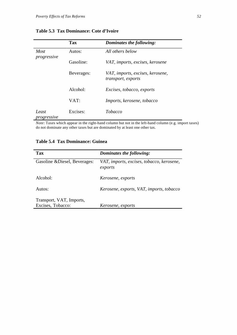
Poverty Effects of Tax Reforms 52
Table 5.3 Tax Dominance: Cote d’Ivoire
Tax Dominates the following:
Mostprogressive
Autos: All others below
Gasoline: VAT, imports, excises, kerosene
Beverages: VAT, imports, excises, kerosene,transport, exports
Alcohol: Excises, tobacco, exports
VAT: Imports, kerosene, tobacco
Leastprogressive
Excises: Tobacco
Note: Taxes which appear in the right-hand column but not in the left-hand column (e.g. import taxes)do not dominate any other taxes but are dominated by at least one other tax.
Table 5.4 Tax Dominance: Guinea
Tax Dominates the following:
Gasoline &Diesel, Beverages: VAT, imports, excises, tobacco, kerosene,exports
Alcohol: Kerosene, exports
Autos: Kerosene, exports, VAT, imports, tobacco
Transport, VAT, Imports,Excises, Tobacco: Kerosene, exports

Poverty Effects of Tax Reforms 53
Table 5.5 Tax Dominance: Madagascar
Tax Dominates the following:
Gasoline, Transport: All others below except autos
Autos: All others below except tobacco
Transport, Excises, Gas intransport, alcohol: Imports, kerosene
VAT, Petroleum, Imports:Kerosene
Table 5.6 Tax Dominance: Tanzania
Tax Dominates the following:
Gasoline & Transport: All others below
Alcohol: Sales, imports, kerosene
Excises, Sales, Imports, Tobacco: Kerosene
Table 5.7 Welfare Ranking of Indirect Taxes in India
Levels of inequality aversion, εCommodity Effective
tax rate0 0.1 1 2 3
Cereals -0.052 8 7 2 2 2Milk, dairy prods. 0.009 9 9 9 9 9Edible oils 0.083 6 6 4 4 5Meat, fish, eggs 0.014 7 8 6 5= 4Sugar, gur 0.069 5 5 5 5= 6Other foods 0.114 4 3 3 3 3Clothing 0.242 1 1 7 7 8Fuel and light 0.274 2 2 1 1 1Other non-food 0.133 3 4 8 8 7

Poverty Effects of Tax Reforms 54
Chapter 6 Analytical Frameworks for Analysing Poverty Impacts of Tax Reform
The evidence on tax incidence in developing countries discussed in chapter 5 was
grouped into five approaches. There are merits and problems associated with each
method, but a probable ranking, from most difficult to apply to easiest, would be:
1) CGE models
2) marginal social cost analysis
3) tax progressivity measures (concentration curves, dominance tests, etc)
4) fiscal simulation models
5) tax progression measures
All of these methods could be usefully applied to poverty analyses of taxes or tax
reforms. The suitability of each for policy advice often hinges on the scope of the
desired poverty assessment, the nature of the reform being considered (e.g. how
narrowly focused or widespread it is), the availability of relevant data, and the
resources available to be committed to the exercise. The best approach for DFID is
probably to seek compromises between more comprehensive methods, with their
extensive data requirements, and/or complex computational procedures, and simpler
methods that are more readily applied to limited data. Below, are the main pros and
cons of each method.
6.1 Alternative Methods
Methods 1 and 2: CGE and MSC analysesThese are probably beyond the scope of investigators without tested computable
models designed for the country or countries in question. However, increasingly CGE
models are being created for individual LDCs which (even if not constructed to
examine fiscal issues) may be adaptable for this purpose. Relevant authors could be
commissioned to undertake tax-poverty assessments. Both methods, however, work
best with data at a fairly high degree of disaggregation and, as a result, price response
information may not be reliable. For this and other reasons it can be difficult to assess
the reliability of any of the scenarios produced. The data requirements of MSC
analyses are significantly less than those of CGE.

Poverty Effects of Tax Reforms 55
Methods 3 to 5 are probably the most feasible for DFID economists (or consultants) to
pursue to assess the poverty impacts of tax reforms in specific country contexts. Below
we outline, in reverse order, how these methods can be applied.
Method Pros Cons
1. CGE - can examine variety ofincidence assumptions
- can examine sector/ socio-economic divisions
- includes behavioural responses- various welfare measures
- data intensive- imposes parameters- smooth price adjustment assumptions
not always appropriate- requires behavioural data
2. Marginalsocial cost
- less data intensive than CGE- behaviour responses via
aggregate price responses- limited welfare measure
- requires behavioural data (priceelasticities)
- marginal changes only- mainly for expenditure taxes- results tend to be sensitive to
inequality aversion3.
ent measuremInequality
ance doWelfare curves
ion Concentrat
min
- can compare pre- & post-reform distributions
- can focus on poverty groups- needs limited data (expend.,
income distribution by group)- apply to direct & indirect taxes- can examine tax compliance- software available ‘off the
shelf’- no (or limited) behavioural
responses
- interpreting crossing curves- statistical tests can have low power- need good data at low incomes to
calculate Ginis etc for poor groups- limited ability to alter incidence
assumptions- no behavioural responses
4. Fiscal simulation
- as above; plus- can generate income distrib-
ution data- can include or exclude
behavioural responses- can report poverty indices- can simulate alternative
incidences
- not previously applied to LDCs,therefore limited knowledge ofmethod’s weaknesses in this context
- only ‘impact effects’ withoutbehavioural assumptions
- software available but needs someadapting to LDC conditions
5. Tax progression
- requires only data on taxstructures
- simple to interpret
- measures tax rates by incomelevel/group but not distributional orpoverty impacts
- welfare interpretations not alwayspossible
- cannot readily adapt incidenceassumptions
- can be misleading re progressivity iffew taxpayers at some tax rates
Method 5: Tax Progression
This essentially requires knowledge of the various tax rates, exemptions and thresholds
and data on actual tax collections. Where the latter are not available by income group,
it is not possible to estimate tax progression for indirect taxes unless household
expenditure data are available by income groups (see below). Also for indirect taxes, it
is the amount of tax as a share of expenditure, not income, which should be used to

Poverty Effects of Tax Reforms 56
calculate tax rates. Tax progression indices are the easiest to calculate and it is easy to
focus on the poorest income groups if desired. This was the approach followed by most
‘first generation’ incidence studies; it can provide a quick guide to potential
progressivity. However, care is needed in interpretation, since it can give a false
picture of distributional effects without knowledge of how many taxpayers pay each
tax rate. For indirect taxes such as sales taxes with exempt items, marginal tax rates
can be difficult to calculate accurately. Tax progression evidence using statutory tax
rates for income taxes is regarded as especially unreliable.
Method 4: Fiscal simulationsThree fiscal simulation approaches are possible, two to examine indirect taxes (trade
taxes, excises, sales taxes etc) and one which examines both personal income and
indirect taxes. All require data from a household expenditure survey (HES) or
equivalent.
In the simplest approach HES data are organised (by income and/or household group)
into items subject to different rates of indirect tax, for example, in the form of an Excel
matrix of total expenditure and expenditure shares for taxed and untaxed items. An
illustration for the UK is shown in Table 6.1. This uses income deciles and items are
arranged in 10 groups of expenditure items facing different tax rates in the UK system:
items subject to VAT at a ‘standard rate’, at 0% and at 5% (insurance, domestic fuel),
alcohol etc. Since these HES data are arranged by income decile, when the tax rates in
column 2 are applied to the expenditure data, the resulting average tax rates provide a
measure of progressivity, not just progression. Statutory tax rates are used in Table 6.1,
but where information on actual collections is available or can be simulated,
corrections can be made to reflect tax compliance. Table 6.1 shows that, for the UK,
while overall indirect taxes are roughly proportional this is made up of a mixture of
progressive (wine excise) and regressive (domestic fuel) taxes. Impacts on poor groups
can be gauged from the lowest deciles.
Alternative incidence assumptions can be examined by this method if data are
available, or plausible scenarios can be identified. For example, if it is believed that the
majority of purchases by consumers in the lowest two deciles are made in the informal
sector (and therefore are untaxed), this can be factored into the spreadsheet. Examining
the incidence of import taxes (for goods that are also produced domestically) is more

Poverty Effects of Tax Reforms 57
difficult because expenditure data does not normally distinguish the source of supply.
However, a combination of input-output (I-O) tables and import data can often provide
a reasonable assessment of import consumption by income levels. Sensitivity testing of
alternatives is usually worthwhile, since theory suggests the prices of perfect
substitutes should be equal whether all are taxed or not.
Two fiscal simulation models (with assorted variants) have been created by John
Creedy of the University of Melbourne, Australia. The first (‘DAWES’ – Demand And
Welfare Effects Simulator) can analyse the welfare, inequality or poverty dimensions
of indirect taxes and reform, and incorporates demand responses to the price changes
induced by tax changes. (The method is described in Creedy, 1999; the main elements
of the programme are in Annex 2). The second, and simpler, programme (‘FLEXI’)
analyses the ‘built-in flexibility’ of taxes; that is, average and marginal rates of tax and
tax elasticities (the proportionate change in tax revenue) across income levels (see
Creedy and Gemmell, 1998; 2001b for Australian and UK applications). This
programme evaluates both income and expenditure taxes, simulates an income
distribution, and can identify tax progressivity measures for the whole income
distribution, for selected groups (e.g. below some poverty threshold) or at specified
income levels.
The input data required are shown in Table 6.2. This shows that ‘effective’, rather than
nominal, income tax allowance/deductions can be incorporated which could be used to
capture evasion aspects. Also the income-expenditure relationship (shown as C = c (Y
– a) in the table) allows for effects of savings differences across income levels and any
other factors which change the reported proportion of disposable income available for
expenditure (such as evasion). Statutory indirect tax rates can be modified to reflect
compliance if desired. To simulate progressivity, additional input files for total
expenditure and budget shares are used. An illustration of average and marginal tax
rate outputs for the UK is shown in Figure 6.1. This indicates, not surprisingly in the
UK case, that the income tax is progressive at all income levels (ATRy). All indirect
taxes combined (ATR*v) are approximately proportional. The (apparently regressive)
ATR v curve however, shows the ATR measured as a proportion of gross income,
indicating the possibilities for misinterpretation if indirect tax liabilities are not
measured with respect to expenditure. These results also confirm that using actual

Poverty Effects of Tax Reforms 58
distribution data in Table 6.1 and the simulated distribution in Figure 6.1 yield similar
estimates.
Neither approach allows for demand responses. When examining tax changes, this
method is best interpreted (like method 3) as measuring ‘impact effects’. To the extent
that behavioural responses are thought likely to be small, however, these simulations
provide a ‘benchmark scenario’ for longer-term effects of reform. Alternative
‘effective’ tax rates and compliance rates can of course be imposed for each tax reform
simulation examined.
Method 3: Concentration curves, inequality indices etc.
Calculation of Lorenz and concentration curves, Atkinson and Gini coefficients,
dominance testing and a wide range of other measures, can readily be performed using
the “DAD4.0” software provided by Jean-Yves Duclos and colleagues at the
University of Laval in Canada. This method requires income or expenditure
distribution, or tax payment, data arranged in a DAD spreadsheet such as that shown in
Figure 6.2. Thus, for example, using the budget share data in Table 6.1, together with
the relevant tax rates, allows shares of tax revenues for each income decile to be
obtained. These can be inserted into the DAD spreadsheet, from which concentration
curves can be obtained from the “curves” pull-down menu shown. As with the above
methods, indices, specific to poor groups can be calculated. Alternative incidence
assumptions can be examined by first building these into the data spreadsheets as in
Method 4. If desired, these Atkinson, Gini etc measures can be used in an abbreviated
social welfare function, where mean income and equality measures (suitably weighted
for the poor) are multiplied together, as discussed in chapter 4. Pre- and post-reform
regimes can be assessed by comparing these abbreviated SWFs.
6.2 Conclusions
Choosing between the methods discussed above will obviously depend on the
availability of data, the country and particular tax scenario being investigated, and so
on. There is no unambiguously preferred technique. Testing incidence assumptions is
possible with most methods, but in all cases the challenge is to know which of these
most accurately depict reality.
Poverty Effects of Tax Reforms 59
Tax progression methods provide a useful ‘first pass’ at potential progressivity of
taxes, but should be complemented wherever possible by either the concentration
curve/dominance testing/Gini measures for which the DAD software is available, or by
the use of fiscal simulations. The merit of this last approach is that it can be applied
with limited data but can also use more sophisticated methods where data allow.
However, it has not so far been applied to LDC conditions.

Poverty Effects of Tax Reforms 60
Table 6.1 Illustrative Excel Example: the UK
Income decile: first second third fourth fifth sixth seventh eight ninth tenth AllBudget shares tax rateVAT exempt 0.00 0.39 0.41 0.39 0.36 0.36 0.34 0.33 0.32 0.31 0.31 0.33standard VAT 0.15 0.44 0.42 0.45 0.48 0.48 0.50 0.52 0.54 0.55 0.57 0.52insurance 0.05 0.01 0.01 0.02 0.02 0.02 0.02 0.02 0.02 0.02 0.01 0.02beer 0.32 0.03 0.02 0.02 0.03 0.03 0.03 0.03 0.02 0.03 0.02 0.02wines 0.53 0.01 0.01 0.01 0.01 0.01 0.01 0.01 0.01 0.01 0.01 0.01spirits 0.64 0.01 0.01 0.01 0.01 0.01 0.01 0.01 0.01 0.01 0.00 0.01other alcohol 0.42 0.00 0.00 0.00 0.00 0.00 0.00 0.00 0.00 0.00 0.00 0.00tobacco 0.82 0.03 0.03 0.03 0.02 0.02 0.02 0.02 0.01 0.01 0.01 0.02petrol 0.86 0.02 0.03 0.03 0.04 0.04 0.04 0.04 0.04 0.04 0.04 0.04domestic fuel 0.05 0.07 0.07 0.06 0.04 0.04 0.03 0.03 0.03 0.02 0.02 0.03
Total expenditure(£ per wk) 119.7 146.8 178.1 244.8 300.0 361.8 412.9 481.8 565.2 782.5 359.4Decile expenditure shares 0.03 0.04 0.05 0.07 0.08 0.10 0.11 0.13 0.16 0.22Total tax payment (£) 15.73 19.33 24.56 35.14 43.97 54.40 62.19 72.40 84.98 110.6 52.37
ATR (all taxes) 0.13 0.13 0.14 0.14 0.15 0.15 0.15 0.15 0.15 0.14 0.15ATR (VAT) 0.06 0.18 0.19 0.21 0.23 0.24 0.26 0.28 0.29 0.31 0.30ATR (wines) 0.003 0.003 0.003 0.004 0.004 0.004 0.005 0.005 0.006 0.007 0.005ATR (dom. fuel) 0.003 0.003 0.003 0.002 0.002 0.002 0.001 0.001 0.001 0.001 0.001
Table 6.2 Input Data for ‘FLEXI’ Simulation Programme
____________________________________________________________________
Income distribution9.5825 0.4560 initial mean and variance of log income
Income tax3; 1999 number of thresholds ;year0.1, 0.23, 0.4 marginal tax rates4335, 5835, 32335 tax thresholds0.25 elasticity of allowance/deductions w.r.t. income
Expenditure-income relationship0.95, 4000 parameters, c and a, of expenditure-income
relationship: C = c(Y+a)
Expenditure taxesindirect tax rates for 10 commodity groups.0000 .1750 .0500 .4706 1.1277 1.7778 .8244 4.5556 6.1429 .0500
Income growth parameters (for time-series simulation)1.0; 0.03; 0.0 beta (for income changes; see note below); growth
rate of income; indexation rate1999 budget share year10 number of periods (of increasing incomes)
Note: Income changes can allow for non-equiproportionate changes inincomes. Hence beta=1 gives equal proportionate changes in incomes;beta<1 implies equalising changes; beta>1 implies disequalisingchange._____________________________________________________________________

Poverty Effects of Tax Reforms 61
Figure 6.1 Tax Progressivity by Income Level (UK, 1999)
0
0.1
0.2
0.3
0.4
5 0 0 0 1 0 0 0 0 1 5 0 0 0 2 0 0 0 0 2 5 0 0 0 3 0 0 0 0 3 5 0 0 0 4 0 0 0 0 4 5 0 0 0 5 0 0 0 0 1 0 0 0 0 0
A T R y
A T R v
ATR*v
I n d i v i d u a l i n c o m e
TaxRate
Figure 6.2 The DAD Spreadsheet

Poverty Effects of Tax Reforms 62
Chapter 7 Conclusions and Policy Recommendations
The objective of this report is to consider how tax systems and tax reforms in
developing countries impact on poverty. To provide some background, chapter 2
reviewed tax systems in developing countries and the characteristics of tax reform
programmes. A summary assessment of this is in section 2.3. Conclusions drawn at the
end of earlier chapters will not be repeated here. Section 3.3 summed up the
prescriptions from tax theory which are relevant to developing countries; section 4.6
drew some conclusions concerning which tools might best be used in tax-poverty
assessments; and section 5.7 summarised the available evidence to date. Chapter 6 has
also suggested possible frameworks and tools that might be used to measure the
poverty impacts of taxation. Some of these are viable using available software and with
limited data. They allow traditional incidence assumptions – which have been
criticised – to be altered for LDC contexts, but to a limited degree. It is also important
to remember that there is very little evidence available to allow the accuracy of
alternative incidence assumptions to be checked. We sum up by addressing a number
of questions and making a set of policy recommendations.
As the focus has been on taxes that affect the poor, directly or, more often, indirectly,
some types of taxes have received little or no attention. The poor are not liable for
personal income tax - even in the rare cases that they earn formal incomes, these will
not exceed the threshold. Thus, the case for income tax reforms is based on efficiency
and equity considerations, and is not in itself an instrument of a poverty reduction
strategy. Similarly, corporate income (profits) taxes or capital taxes (on inheritances or
capital gains) are unlikely to have even an indirect effect on the poor, and hence have
been excluded from consideration. The same applies to property taxes: while desirable
for equity reasons, they are not incident on the poor (although they could be passed on
to tenants) and rarely used in LDCs.
We have not considered local taxes, largely because there is very little evidence
available, these are rarely the subject of tax reform discussions, and practices vary
considerably. However, it is worth mentioning that some countries have poll taxes as a
means of raising revenue. While these are usually at very low, and not always uniform,
rates, the presumption would be that they are regressive. In fact, this may not be the

Poverty Effects of Tax Reforms 63
case. Fjelstad and Semboja (2001) discuss the development levy, a local poll tax in
Tanzania, and reach two conclusions of relevance here. First, compliance rates are
higher for those on higher incomes because they are involved in more visible activities
(such as trade), so the tax is progressive. Second, taxpayers are more willing to comply
if they can see that public services are being provided. This emphasises the important
role that aid finance for the provision of public services (especially visible pro-poor
services such as education, health and sanitation) can play during the tax reform
process.
Taxpayers are more willing to comply if public services are being provided. In the pre-
reform stage, total revenues are low (hence constraining the level of services provided)
and collection is inefficient (due to corruption by tax administrators and evasion by
taxpayers). Tax reform is associated with two types of uncertainty, both of which can
be reduced by aid inflows. First, governments are uncertain of the effects on revenue;
this is one major reason for implementation failure of trade tax reforms (see Morrissey,
1995). Second, administrative changes imply statutory uncertainties that increase the
scope for evasion (this provides an argument for relatively simple reforms). If aid is
used to maintain revenues, supporting government commitment, and to finance public
services, increasing the incentives for taxpayers to comply, it can support the reform
process. We return to this point in the policy implications.
1. Do any reliable analytical results emerge for the design/reform of ‘efficient’
revenue systems in LDCs?
Section 3.3 provided some answers to this question. In essence, the answer is that
analytical results do emerge, but they depend on the range of tax instruments available
to the government and whether all goods/sectors/households can be taxed. In poorer
countries where income taxes are limited and agricultural/informal sectors cannot
readily be taxed directly, the common ‘tax neutrality’ advice for tariffs and domestic
indirect taxes derived from theory is not appropriate. This is reinforced when equity
considerations are part of the objectives of the tax system. However, arguments for
varying sales/excise tax rates must be treated cautiously. Indirect taxes are blunt
instruments for redistribution to the extent that both rich and poor consume similar
goods. Where they consume different goods, it is possible to target indirect taxes better
than poorly administered and evaded direct taxes. A case for neutrality as representing

Poverty Effects of Tax Reforms 64
a simple tax structure that reduces incentives for evasion can be made, based more on
the realities of poor administration services and corruption. The general
recommendation is for few relatively low tax rates.
2. Does the analysis/evidence generate robust findings on the distributional and
poverty impacts of taxes and/or reform?
Robust findings are quite hard to find, in part because for many countries or taxes only
one or two methods have been used to examine redistribution, often adopting similar
incidence assumptions. There is a dearth of comparable country studies. Two results do
appear with some regularity:
a) trade and sales taxes (e.g. VAT) may not be ‘regressive’ as typically found in early
studies. This partly results from the deficiencies of early methods, and from the fact
that numerous anomalies in these tax rates have been removed by reforms. Recent
studies tend to find trade and sales taxes to be progressive, if only mildly. Since
many reforms involve replacing trade taxes with VAT or similar sales taxes, an
interesting issue is whether the ‘new’ taxes are more pro-poor. Results here seem to
be country specific. In some studies VAT is more progressive than tariffs and/or
excises, but the reverse is true in others. It seems that progressivity measures for
these taxes are often very close so that ‘not much changes’ with this aspect of
reform. Effects on the poorest of most such tax reforms are likely to be small.
b) the most robust results appear to be the regressivity of fuel taxes such as kerosene
and export taxes such as those on cocoa and coffee. While taxes on intermediates
such as fuel are often thought to be regressive because they affect transport costs
for the poor, evidence so far does not confirm this. Rajemison and Younger (2001)
find that allowing for this effect does not make implicit transport taxes regressive
in Madagascar, while Chen et al (2001) find, for Uganda, that progressivity is
reduced but not reversed. This does not mean that the poor are not affected by these
taxes – there can be sizeable effects – but they do not fall disproportionately on the
poor.
In general, most evidence does not examine poverty effects of taxes directly, but
focuses on broader inequality effects; at best, one can infer effects on the poor, on the
assumption that more pregressive taxes are more pro-poor. The general verdict for
Poverty Effects of Tax Reforms 65
Africa seems to be that expenditures are very unequally distributed, but taxes (with the
exceptions noted above) have relatively little impact on this.
3. Can, and should, tax systems be reformed to make them more progressive?
The evidence suggests that some aspects of current tax systems in LDCs could be
reformed to make them more progressive. The removal of highly regressive excises is
one example, reducing the level and dispersion of trade taxes is another. However,
some progressivity enhancing reforms would undoubtedly have distortionary effects
and/or be administratively difficult. Great care needs to be taken in assessing (a) the
potential extent of these; and (b) the necessary value judgements required before the
required compromises can be recommended. As Chu et al (2000, p.37) put it: ‘if the
progressivity of the tax system were achieved at the cost of revenue, relative to the
case of a neutral tax regime, the gains in redistribution on the tax side could be more
than offset by the lost opportunities to use progressive expenditure policy instruments’.
Where public expenditures can be targeted at the poor they are likely to provide a more
potent, and less distorting, anti-poverty instrument than a highly non-proportional tax.
4. How reliable are existing methods for assessing poverty impacts of taxation?
There are now a variety of methods available. Tax progression studies are possibly the
least reliable (at least, early versions) because they rely only on an examination of
statutory tax rates. Shah and Whalley (1991) argue that ‘traditional’ incidence
assumptions lead to misleading results for LDCs, especially for indirect taxes. But
even using (close to) traditional assumptions, recent evidence is more supportive of
‘mildly progressive’ indirect taxes (more radical changes of incidence assumptions
also produce this revision). It is therefore hard to make a judgement on the reliability
of methods, but improving data availability is encouraging for empirical analysis. So
long as data on such aspects as informal sector expenditures is limited it will be
difficult to know how well these aspects are captured by current practice.
Chapter 6 suggested that existing methods can be used by economists engaged in
policy advice provided care is taken to check sensitivity to assumptions wherever
possible. Country-specific conditions must also be evaluated carefully. Younger (1996)
provides a pertinent example in Ghana. He found that about 70% of the additional tax
revenues achieved during the 1980s tax reform were accounted for by the highly

Poverty Effects of Tax Reforms 66
regressive cocoa export duty and petroleum excises. This might suggest reform was
bad for the poor. However, cocoa farmers incomes rose during the reform and, before
reform, an overvalued exchange rate meant that there was an implicit tax on exports
(benefiting foreign importers rather than the government). When pre-reform taxes are
adjusted to reflect this it turns out that reform actually reduced reliance on the
regressive cocoa duty. This highlights the importance of considering implicit tax
incidence carefully.
5. Can tax reform contribute to a poverty-reducing growth strategy?
The answer to this question is ‘yes’. Existing evidence points to examples (even in tax
systems that have undergone reforms) of taxes which either distort behaviour or
adversely affect the poor or both. Reforming these taxes can help to facilitate growth
and reduce poverty. Most export taxes seem to fall into this category. However in
countries that rely heavily on export revenues to finance expenditures it will be
important to ensure that revenue losses are avoided. If not, the adverse effects of the
inflation tax on the poor will ensue. Equally important is the type of tax which replaces
export revenues. If this is simply achieved by raising taxes which are regressive (such
as some excises) on goods in inelastic demand, it may simply substitute adverse effects
on one poor group to benefit another. Alternatively, if revenues are increased from
progressive taxes, care must be taken not to distort incentives such that growth
objectives are undermined.
In general, the role of tax reforms in Poverty Reduction Strategy Papers (PRSPs)
should depend on how effectively poverty can be targeted by social expenditures.
Where this is effective, it may be best to restrict tax policy to making the tax system no
more than mildly progressive, but maximise its administrative and economic
efficiency. In these cases, approximate tax neutrality is probably a reasonable policy.
Over the longer term LDCs will have to raise their tax/GDP ratios if increases in
poverty-reducing expenditures are to be financed from domestic rather than aid
resources. This will require careful thought concerning which taxes should provide the
additional resources, and this will vary from country to country. However, it seems that
broad-based sales taxes such as VAT are not generally regressive in most LDCs, in
part because of the use of exemptions and two or three tax rates. It is generally not
desirable to make these taxes strongly progressive, but they can be designed to avoid

Poverty Effects of Tax Reforms 67
hurting the poorest. With reforms to regressive excises and tariffs, improvements in tax
administration over time, and a readiness to expand income taxation as practicalities
allow, tax reforms should be capable of delivering increasing revenues without
adversely affecting the poorest. Finding ways of taxing richer producers in agriculture
other than through export taxes (which seems to hurt poor farmers more) is one
challenge for future tax reform. Greater use of rural property taxation may be an option
that avoids excessive distortions, but this has proved politically difficult to implement
in the past.
Policy Recommendations for Pro-Poor Tax Reform
In the light of the answers to the preceding five questions, and given the evidence
reviewed in earlier chapters, there are a number of concluding recommendations to
enhance the pro-poor potential of tax reform, so that the burden on the poor is reduced
or, at least, not increased. While the general principle from standard theory for
commodity taxes (sales and trade) is to levy a uniform rate (tax neutrality), we have
argued that there good reason to deviate from this principle in LDCs. The first three
recommendations refer to such deviations, the remainder are more general.
Ø Commodity taxes, both on sales and trade, should have few rates with a low
dispersion. A simple sales tax is more appropriate than a complex VAT, and
excises should be levied on an ad valorem rather than fixed charge basis. Tax rates
should be higher on goods with inelastic demand as factors are not fixed, some
sectors cannot be taxed directly and the range of tax instruments is limited.
Ø Commodity taxes can be made pro-poor by ensuring zero rates on goods that are
consumed predominantly by the poor rather than the rich, and on activities that are
engaged in predominantly by the poor. As the poor predominate in the informal
sector, one would not tax informal sector activities, or complementary activities.
Similar arguments apply to subsistence agriculture.
Ø A strong case can be made to subsidise the price of commodities that are consumed
by the poor but not by the rich (e.g. kerosene, some staple foods). While there are
well known problems of targeting subsidies accurately, the benefits to the poor are

Poverty Effects of Tax Reforms 68
likely to outweigh the possibility that some of the non-poor will benefit. This is the
only recommendation that differs from standard IFI fiscal policy recommendations.
Ø Reducing the dispersion and average level of tariff rates is pro-poor, largely
because tariff reductions lower taxes on intermediate inputs and reduce the
effective taxation of agriculture.
Ø A more simple tax structure (fewer and lower rates) contributes to collection
efficiency and economic efficiency. Economic efficiency is greater because relative
price distortions are reduced. Collection is more efficient because simple taxes are
easier to administer and the incentives to evade are less. Consequently,
simplification of tax structures usually increases revenue.
Ø A relatively simple income tax is progressive. The threshold exemption is in effect
a lump-sum transfer that provides for progression, while having few tax rates
reduces the disincentive effects. However, income taxes are not incident on the
poor, and are thus not a core element of a pro-poor tax reform strategy.
Sometimes the obvious can bear re-stating. In LDCs, especially the poorest, tax
administration capacity is severely limited – staffing levels are low, wages are low, and
resources are limited – while the culture of tax evasion is well-established. Simple tax
reforms, and reforms that introduce more simple tax structures, are not only the most
feasible, they are also likely to increase revenue. Political capacity to implement
reforms is also weak, while domestic political opposition is likely to be strong (both
from those facing increased taxes and from those losing protection as tariffs are
reduced). The reform process itself introduces uncertainties that constrain
implementation capacity and provides incentives for opponents of reform and would-
be evaders to exploit. Aid support from donors, to ensure provision of public services
and provide technical support for administering reforms, is a vital component of a
successful reform programme.

Poverty Effects of Tax Reforms 69
References
Adam, C. and D. Bevan (2001), Fiscal Policy Design in Low-Income Countries, UNU/WIDER
Discussion Paper No. 2001/67. Helsinki: WIDER.
Ahmed, E. and Stern, N. (1984) ‘The theory of tax reform and Indian indirect taxes, Journal of
Public Economics, 25, 259-298.
Ahmed, E. and Stern, N. (1987) ‘Alternative sources of government revenue: examples from
India, 1979-80’ in Newbery and Stern (eds).
Ahmad, E. and Stern, N. (1989) ‘Taxation for developing countries’, in H. B. Chenery and T.
N. Srinivasan (eds), Handbook of Development Economics, volume 1. Amsterdam: North
Holland.
Ahmed, E. and Stern, N. (1991) The Theory and Practice of Tax Reform in Developing
Countries. Cambridge: Cambridge University Press.
Atkinson, A.B. (1970) ‘On the measurement of inequality’, Journal of Economic Theory, 2,
244-263.
Barbone, L. Das-Gupta, A., De Wulf, L. and Hansson, A. (1999) Reforming Tax Systems: The
World Bank Record in the 1990s. Tax Policy and Administration Thematic Group.
Washington: The World Bank, processed.
Bird, R. (1992) Tax Policy and Economic Development. Baltimore and London: Johns Hopkins
University Press.
Burgess, R. and N. Stern (1993), ‘Taxation and Development’, Journal of Economic
Literature, 31, 762-830.
Chen, D., Matovu, J.M. and Reinikka, R. (2001) A Quest for Revenue and Tax Incidence in
Uganda. IMF Working Paper, WP/01/24. Washington DC: IMF.
Ghia, N.C., Wahba, S. and Whalley, J. (2000) ‘Analysing the incidence of taxes in the Cote
d’Ivoire’ in Bevan, D., Collier, P., Gemmell, N. and Greenaway, D. (2000) Trade and
Fiscal adjustment in Africa. London: Macmillan.
Choon, C.N. (2000) ‘Using a computable general equilibrium (CGE) model to evaluate the
Singapore tax system’, in G. Perry, et al. (eds).
Chu, K., Davoodi, H. and Gupta, S. (2000) Income Distribution and Tax and Government
Social Spending Policies in Developing Countries. IMF Working Paper No. WP/00/62.
Washington DC: IMF.
Clarete, R.L. (1991) ‘A general equilibrium analysis of the tax burden and institutional
distortions in the Philippines’ in J. Khalilzadeh-Shirazi and A. Shah (eds). Tax Policy in
Developing Countries. Washington DC: World Bank.
Coady, D. (1997), ‘Fiscal Reform in Developing Countries’, in C.K. Patel (ed).

Poverty Effects of Tax Reforms 70
Coady, J. and Harris, R.L. (2001) Evaluating Transfer Programs within a General Equilibrium
Framework. FCND Discussion Paper No. 100. Washington DC: IFPRI.
Creedy, J. (1998a) The Dynamics of Inequality and Poverty. Comparing Income Distributions.
Cheltenham: Edward Elgar.
Creedy, J. (1998b) Measuring Welfare Changes and Tax Burdens. Cheltenham: Edward Elgar.
Creedy, J. (1999) Modelling Indirect Taxes and Tax Reform. Cheltenham: Edward Elgar.
Creedy, J. (2001) Taxation and Economic Behaviour. Cheltenham: Edward Elgar.
Creedy, J. and Gemmell, N. (1998) ‘The built-in flexibility of taxation: some basic analytics’.
University of Melbourne, Department of Economics, Research Paper No. 628, Melbourne
University.
Creedy, J. and Gemmell, N. (2001a) ‘The built-in flexibility of income and consumption taxes:
a survey’, in J. Creedy (ed), Taxation and Economic Behaviour. Cheltenham: Edward
Elgar.
Creedy, J. and Gemmell, N. (2001b) The Revenue Elasticity of Taxes in the UK. University of
Melbourne, Institute of Applied Economic and Social Research, Working Paper No. 11/01,
Melbourne: MIAESR.
Dahl, H and Mitra, P. (1991) ‘Applying tax policy models in country economic work:
Bangladesh, China and India’ in J. Khalilzadeh-Shirazi and A. Shah (eds). Tax Policy in
Developing Countries. Washington DC: World Bank.
Dean, J., Desai, S. and Riedel, J. (1994), ‘Trade Policy Reform in Developing Countries Since
1985: A Review of the Evidence’, The World Bank (mimeo).
Devarajan, S. and Panagariya, A. (2000) ‘The theory and practice of trade reform: a public
economics perspective’, in G. Perry, et al. (eds).
Diamond, P.A. (1975) ‘A many-person Ramsey tax rule’, Journal of Public Economics, 4,
335-342.
Duclas, J-Y., Araar, A. and Fortin, C. (2001) DAD: Distributive Analysis. User’s Manual.
University of Laval, Canada. (Available at www.mimap.ecn.ulaval.ca).
Fjelstad, O. and J. Semboja (2001), ‘Why people pay taxes: the case of the development levy
in Tanzania’, World Development, 29, 2059-75.
Foster, J., Greer, J. and Thorbecke, E. (1984) ‘A class of decomposable poverty measures’,
Econometrica, 52, 761-2.
Gemmell, N. (1987) ‘Taxation and development’, in N. Gemmell (ed) Surveys in Development
Economics. Oxford: Basil Blackwell.
Greenaway, D. and C. Milner (1991), ‘Fiscal Dependence on Trade Taxes and Trade Policy
Reform’, Journal of Development Studies, 27: 2, 95-132.
Gupta, S., Davoodi, H and Alonso-Terme, R. (1998) Does Corruption Affect Income Inequality
and Poverty? IMF Working Paper No. WP/98/76. Washington: IMF.

Poverty Effects of Tax Reforms 71
Heady, C. (1987) ‘A diagramatic approach to optimal commodity taxation’, Public Finance,
42, 250-263.
Heady, C. (1993) ‘Optimal taxation as a guide to tax policy: a survey’, Fiscal Studies, 14, 15-
41.
Heady C. (2001) Taxation Policy in Low-Income Countries. UNU-WIDER Discussion Paper
No. 2001/81. Helsinki: WIDER.
Heady, C. and Mitra, P.K. (1987) ‘Distributional and revenue raising arguments for tariffs’,
Journal of Development Economics, 26, 77-101.
Hindricks , J., Keen, M. and Muthoo, A. (1999) ‘Corruption, extortion and evasion’, Journal of
Public Economics, 74, 395-430.
IMF (2001) Structural Conditionality in Find-Supported Programs. Washington DC: IMF.
Jenkins, G.P. and Kuo, C-Y. (2000) ‘A VAT simulation model for tax reform in developing
countries’, World Development, 28, 763-774.
Jenkins, S.P. (1988) ‘Empirical measurement of horizontal inequity’, Journal of Public
Economics, 37, 305-329.
Jenkins, S.P. and Lambert, P.J. (1997) ‘Three ‘I’s of poverty curves, with an analysis of UK
poverty trends’, Oxford Economic Papers, 49, 317-327.
Jimenez, E. (1986) ‘The public subsidisation of education and health in developing countries: a
review of equity and efficiency, World Bank Research Observer, 1, 111-130.
Lambert, P.J. (1993) The Distribution and Redistribution of Income. Second Edition.
Manchester: Manchester University Press.
Lora, E. and Herrera, A.M. (2000) ‘Tax incidence in Colombia: a general equilibrium analysis’,
in G. Perry, et al. (eds).
Madden, D. (1995) ‘An analysis of indirect tax reform in Ireland in the 1980s’, Fiscal Studies,
16, 18-37.
Madden, D. (1996) ‘Marginal tax reform and the specification of consumer demand systems’,
Oxford Economic Papers, 48, 556-567.
Morrissey, O. (1995), ‘Politics and economic policy reform: trade liberalisation in sub-Saharan
Africa’, Journal of International Development, 7, 599-618.
Newbery, D. and Stern, N. (eds) The Theory of Taxation for Developing Countries. Oxford:
Oxford University Press.
Patel, C.K. (ed) (1997), Fiscal Reforms in the Least Developed Countries, Cheltenham: Edward
Elgar.
Perry, G., Whalley, J. and McMahon, G. (eds) Fiscal Reform and Structural Change in
Developing Countries, volumes 1 & 2. London: Macmillan.

Poverty Effects of Tax Reforms 72
Podder, N. (1997) ‘Tax elasticity, income redistribution and the measurement of tax
progressivity’ in S. Zandvakili (ed), Inequality and Taxation. Research on Economic
Inequality, Volume 7. Greenwich, CT, and London: Jai Press.
Rajemison, H. and Younger, S.D. (2001) Indirect Tax Incidence in Madagascar: Estimations
Using the Input-Output Table. Cornell University Food and Nutrition Program, processed.
Sahn, D.E. and Younger, S.D. (1999) Dominance Testing of Social Expenditures and Taxes in
Africa. IMF Working Paper No. WP/99/172. Washington DC: IMF.
Shah, A. and Whalley, J. (1991) ‘The redistributive impact of taxation in developing
countries’, in J. Khalilzadeh-Shirazi and A. Shah (eds). Tax Policy in Developing
Countries. Washington DC: World Bank.
Stern, N. (1987) ‘The theory of optimal commodity and income taxation: an introduction’, in
Newbery and Stern (eds).
Tanzi, V. (1987) ‘Quantitative characteristics of the tax systems of developing countries’ in
Newbery and Stern (eds.
Tanzi, V. (1991) Public Finance in Developing Countries. Cheltenham: Edward Elgar.
Tanzi, V. (2000) ‘Taxation and economic structure’, in G. Perry, et al. (eds).
Tanzi, V. and Davoodi, R. (2000) Corruption, Growth and Public Finances. IMF Working
Paper No. WP/00/182. Washington DC: IMF.
Tanzi, V. and Zee, H.H. (2000) Tax Policy for Emerging Markets: Developing Countries. IMF
Working Paper No. WP/00/35. Washington DC: IMF.
Thirsk, W. (ed) Tax Reform in Developing Countries. Washington DC: World Bank.
Van de Walle, D. and Nead, K. (1995) Public Spending and the Poor. Theory and Evidence.
Washington DC: World Bank.
Webb, S. and K. Shariff (1992) ‘Designing and Implementing Adjustment Programs’, in V.
Corbo, S. Fischer and S. Webb (eds), Adjustment Lending Revisited: Policies to Restore
Growth, Washington DC: The World Bank, pp 69-92.
World Bank (1999), World Development Report 1998/99, Washington DC: World Bank.
World Bank (2000), World Development Indicators 2000, Washington DC: World Bank.
Yitzhaki, S. and Slemrod, J. (1991) ‘Welfare dominance: an application to commodity
taxation’, American Economic Review, 81, 480-496.
Younger, S.D. (1996) ‘Estimating tax incidence in Ghana using household data’, in D. Sahn
(ed), Economic Reform and the Poor in Africa. Oxford Clarendon Press.
Younger, S.D., Sahn, E.S., Haggblade, S. and Dorosh, P.A. (1999) ‘Tax incidence in
Madagascar: an analysis using household data’, World Bank Economic Review, 13, 303-
331.

Poverty Effects of Tax Reforms 73
Annex 1 Two Tax Reform Examples: Kenya and Mauritius
Oliver Morrissey
This annex considers two different cases of tax reform: Kenya and Mauritius. Kenya is
a ‘lower middle income’ African country (and one that appears to be moving towards
‘low’ rather than ‘middle’) that has a reputation for inconsistent compliance with
successive adjustment programmes since the 1980s. Mauritius is one of the African
successes, having implemented significant policy reforms and grown rapidly since the
1970s. Considering two such diverse examples permits us to draw out contrasting
issues.
Kenya in 2000
A number of important trends in the composition of tax revenue and the implicit tax
rates (revenue collected expressed as a percentage of the relevant tax base) for Kenya
in the late 1990s are summarised in Table A1. Note a general tendency for the
contribution of income taxes to decline (largely due to declining profits, hence less
revenue from corporate profits tax), while the share of revenue from VAT increases
(although food and agriculture are largely exempt). However, although the contribution
of import duties would be expected to decline (as trade policy reforms include reducing
import protection), this trend was reversed in the late 1990s (but is projected to be back
on track in the early 2000’s, heading back towards 16% of revenues).
The estimates of implicit taxes are instructive. Tariffs on inputs (basic materials,
machinery and capital equipment) have been reduced, as have those on transport
equipment, but tariffs on foods, beverages and fuels appear to have increased. This is
noticeable in budgets, since 1998/99 measures have been introduced to raise duty rates
on foods, agricultural produce and substitutes, to 25% in many cases, with suspended
duties imposed on various fruits and vegetables. Although residual fuel duties were
reduced, the tax revenue from fuel remains very high.
Kenya has been implementing a Tax Modernisation Programme since the mid-1980s,
involving restructuring and rationalisation of rates, and measures to improve tax
administration and increase collection efficiency. Many reforms have related to local
Poverty Effects of Tax Reforms 74
taxes, including property taxes, although these do not yet yield significant revenues.
The efficiency of the system has been increased significantly, and distributional
considerations are taken into account. The general approach has been to take a long-
term perspective, with the view that higher growth rates are the best way to deliver
poverty reduction and higher incomes. Thus, tax rates should not be so high as to
discourage private sector activity. Furthermore, business profits are not a reliable
source of revenue both because of declining profitability in recent years and because of
the disincentive effects.
Given the importance of the agricultural sector to the economy, and the concentration
of poverty in rural areas largely dependent on agriculture, the tax treatment of the
agricultural sector has been an issue of major concern. The strategy has reflected twin
objectives of assisting agricultural producers while minimising the taxation of food and
other agricultural products. Basic foods (such as flour, bread and milk) are exempt
from VAT. In general, farmers are exempted from tax registration and subject to
indirect means of taxation. All unprocessed farm products (except coffee and tea) are
VAT exempt. The principal agricultural inputs, such as fertilizers and seeds, are zero
rated for VAT and exempt from import duties.
On the other hand, Kenya has chosen to use trade policy to protect farmers, notably
through tariffs on imports of agricultural products, especially the major grains (maize,
wheat, rice), milk, sugar, fruits and vegetables. The nominal protection on these items
ranges from 25% up to maximum of 100% on sugar although, since October 2000,
imports are duty free (in principle) from COMESA countries. While the motives for
this protection policy are understandable, high tariffs are known not to be the best way
to help achieve this. The predicament, for Kenyan policy and for the PRSP, is that
most measures to increase agricultural output and incentives demand public spending
(on improving transport and marketing, providing improved quality inputs and
technology, and extension services).
Given the prevalence of poverty in poor areas, a pro-poor growth strategy would
clearly include policies to support the development and increased productivity of the
agricultural sector. Tariff protection can be helpful as a sector develops, but can also
support, if not encourage, inefficiency in local production. ‘The inward-oriented
policies in the agriculture sector have led to the development of agri-processing

Poverty Effects of Tax Reforms 75
industries, the major branch of Kenya’s manufacturing sector. Nevertheless,
liberalization reforms have revealed the weaknesses of the intersectoral linkages and
the lack of competitiveness of the manufacturing sector’ (WTO, Trade Policy Review
Kenya, 2000, p.51). It is important to determine why Kenyan agricultural producers
feel that they face unfair competition from (some) imports. If the underlying problem
is low levels of efficiency in Kenyan agriculture, farming and agri-processing, the
appropriate intervention would be support at the production level. This would have
implications for government spending.
A number of measures try to protect the poor from taxes. Unprocessed or basic foods,
medical and health care items are generally exempted, but processed foods are taxed
(these are mostly consumed by middle and higher income households). The poor
generally derive their fuel needs from wood, charcoal and kerosene; the former are not
taxed (but may be over-used) while the latter is lightly taxed. Taxes on petrol and
diesel have not increased in line with the world price so that the effective tax rates on
petrol and diesel have fallen significantly in recent years. Household’s can consume
basic electricity needs without paying VAT. The personal income tax allowance
effectively exempts all low-income individuals (although it fails to capture all the
taxable income of those actually liable).
In addition to the various agricultural products that are subject to high import duties, a
number of other products that form a significant share of the expenditure budget of the
poor are also subject to tariffs. Nominal duty rates are in the range of 30% to 40% for
clothing and textiles, footwear, dry cell batteries (for radios, torches, etc), paper and
paper products, soap, toothpaste, and most metal, plastic and wooden products. These
goods are also subsequently subject to VAT. The high duty rate on clothing has
encouraged a thriving market in used clothing imports (much of which is smuggled)
that tends to benefit the poor; clothing prices have risen much slower than the general
consumer price index in the 1990s. Thus, while some taxes increase the prices of goods
that are important in the consumption bundles of the poor, there is limited scope to
alter the tax structure in a pro-poor manner. Thus, the poor are largely sheltered from
having to pay taxes on their incomes or on the goods they consume.

Poverty Effects of Tax Reforms 76
Mauritius in the 1990s
Mauritius avails of a wide range of taxes. To sketch the composition we take fiscal
year 1990/91, when total tax revenue was some nine billion Rupees, as an example
(see Morrissey, 2001). Income taxes contributed about 15 per cent of total tax revenue,
in the rough proportion 60:40 between corporate and individuals, while social security
contributions and payroll taxes added about another five per cent. Domestic taxes on
goods and services contributed about a quarter of revenue, in rough proportions
40:40:10:10 between excise duties, sales taxes, taxes on gambling and on hotel bills.
Trade taxes contributed 52 per cent of tax revenue; 90 per cent of which is from tariffs
(and export taxes were abolished from 1994/95). The only other major tax is that on
property, which contributes just less than seven per cent of total tax revenue. Non-tax
revenues were equivalent to five per cent of tax revenue and came mostly from
property income, fees, charges and non-industrial services.
A number of general trends are apparent in Mauritius. First, and perhaps foremost, the
country is becoming progressively less reliant on trade taxes, which have declined as a
share of tax revenue from about 60 per cent throughout most of the 1980s, to 50 per
cent in the early 1990s and tending towards 40 per cent in the late 1990s. About half of
this decline is attributable to the reduction and then abolition of export taxes, but
tariffs’ contribution to revenue also seems to be declining. This dependence on trade
taxes implies relatively high levels of effective protection and has adversely affected
resource allocation. Such trade taxes increase the degree of economic inefficiency in
the tax system.
Although nominal tax revenue almost quadrupled between 1985 and 1995, real tax
revenue, as indicated by the tax/GDP ratio, rose only slightly from 20 to about 22 per
cent (there is an one-off fall in tax revenue in 1994/95, apparently associated with the
abolition of export taxes). This is consistent with rising national income, and arguably
the aggregate tax take is about right. Domestic taxes on goods and services are
becoming an increasingly important source of revenue, from just over a fifth of tax
revenue in the early 1980s to almost one third by the late 1990s. This trend is likely to
continue under the VAT. Part of this increase may reflect replacing tariffs with sales
taxes, which would generally imply a reduction in economic inefficiencies associated
with the tax system.

Poverty Effects of Tax Reforms 77
Contributing about 15% of revenues the income tax in Mauritius can potentially
contribute more to redistribution than in most African countries. Table A2 provides
some data on the progression of the individual income tax system in Mauritius for
1992/93 compared with 1994/95 (for illustrative purposes). Three points are worth
making. First, the overall ATR (on the tax base of gross income) falls slightly to just
above seven per cent (allowances and bands probably increased by more than income).
Subsequently, changes to the income tax structure suggest that the ATR will have
increased, perhaps to eight per cent by 1997/98. Second, for both years there are
anomalies in the data: the apparent ATR is relatively high for those earning Rs20-
40,000 in 1994/95, and there is almost certainly some misallocation to the Rs100-
250,000 range from adjacent ranges. (The pattern for 1992/93 is what would be
expected and is similar to the patterns for 1991/92 and 1993/94 (not shown)). Third,
there is a discernible degree of progression: the ATR rises from around 2% to 18%;
and, given an MTR of around 30%, Liability Progression in 1992/93 was roughly 3.9
and in 1994/95 was almost 4.2. This also implies potential buoyancy in the income tax:
as incomes rise, tax revenue should rise more than proportionally,suggesting scope for
income tax to be an increasingly important source of revenue.
The tax system in Mauritius therefore has a number of merits. Income tax appears
relatively equitable, demonstrating progression, and is relatively simple. The principal
anomaly lies in the special treatment of agricultural incomes, especially those in the
sugar sector. The introduction of VAT to replace Sales tax will have transitional costs
but should ultimately lead to more efficient (economically, and in terms of collection)
and buoyant taxation of domestic goods and services. Further moves to reduce and
rationalise tariffs should promote simplicity, economic and collection efficiency; while
the elimination of taxes on exports removes one major distortion. Overall, the changes
to the tax system can be regarded as are moving it towards a more desirable structure,
but much remains to be done.
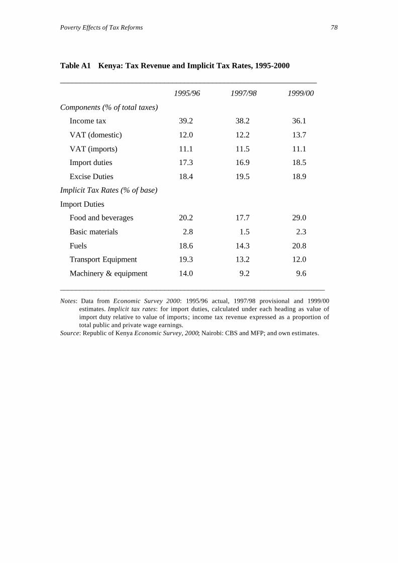
Poverty Effects of Tax Reforms 78
Table A1 Kenya: Tax Revenue and Implicit Tax Rates, 1995-2000
________________________________________________________________
1995/96 1997/98 1999/00
Components (% of total taxes)
Income tax 39.2 38.2 36.1
VAT (domestic) 12.0 12.2 13.7
VAT (imports) 11.1 11.5 11.1
Import duties 17.3 16.9 18.5
Excise Duties 18.4 19.5 18.9
Implicit Tax Rates (% of base)
Import Duties
Food and beverages 20.2 17.7 29.0
Basic materials 2.8 1.5 2.3
Fuels 18.6 14.3 20.8
Transport Equipment 19.3 13.2 12.0
Machinery & equipment 14.0 9.2 9.6
__________________________________________________________________
Notes: Data from Economic Survey 2000: 1995/96 actual, 1997/98 provisional and 1999/00estimates. Implicit tax rates: for import duties, calculated under each heading as value ofimport duty relative to value of imports; income tax revenue expressed as a proportion oftotal public and private wage earnings.
Source: Republic of Kenya Economic Survey, 2000; Nairobi: CBS and MFP; and own estimates.

Poverty Effects of Tax Reforms 79
Table A2 Mauritius: Progression of the Income Tax, 1992/93 and 1994/95
1992/93Gross Income Gross Tax Average
Range (Rs '000s) Income Paid Tax Rate
< 20 5.2 0.1 1.9220 - 30 9.8 0.3 3.0630 - 40 69.0 1.7 2.4640 - 50 184.9 4.0 2.1650 - 100 2060.0 69.4 3.37100 - 250 3063.1 215.5 7.04250 - 500 854.7 116.8 13.67
> 500 790.6 136.3 17.24TOTAL 7037.3 544.1 7.73
1994/95Gross Income Gross Tax Average
Range (Rs '000s) Income Paid Tax Rate
< 20 0.6 0 0.0020 - 30 0.6 0.1 16.6730 - 40 0.8 0.1 12.5040 - 50 108.6 0.3 0.2850 - 100 2320.1 38.3 1.65100 - 250 388.5 235.1 60.51250 - 500 1225.1 155.0 12.65
> 500 1051.5 187.6 17.84TOTAL 8595.8 616.5 7.17
Source: Derived from Table 6.1 in Digest of Public Finance Statistics 1992-1996 , Port-Louis,
Mauritius: Central Statistics Office

Poverty Effects of Tax Reforms 80
Annex 2D emand A nd W elfare E¤ects Simulator
John CreedyThe University of Melbourne
1

Poverty Effects of Tax Reforms 81
1 I nt r oduct ionThis annex describes a set of computer programs that are designed to ex-amine the welfare e¤ects of price changes, allowing for consumers’ demandresponses. Theprograms aredescribed in termsof thegeneral t it le: D emandA nd W elfare E¤ects Simulator - DAWES.
It is possible to examine t he e¤ectsof a speci…ed set of proport ional pricechanges on the compensat ing and equivalent variat ions of each householdin the Household Expenditure Survey (HES), along with t he distribut ionof ‘equivalent incomes’ (money metric welfare measures). Alternat ively thewelfare changes at alternat ive speci…ed levels of t otal expenditure can beobtained. The price changes apply to the commodity groupings used by theHES. The price changes may arise for a var iety of reasons - DAWES onlyrequires the proport ionate changes to be speci…ed. If the pricechanges arisefrom indirect taxes, or changes in indirect taxes, i t isalso possiblet ocomputetax rates that are revenue-neutral in aggregate.
Sect ion 2describes theanalyt ical framework of analysisused. Thevariousprograms and their associated data …les are described in sect ion 3.
2 T he M odell ing Fr ameworkThis sect ion describes theway in which household demandsaremodelled andthe calculat ion of equivalent and compensat ing variat ions.1. The frameworkis one in which the total expendit ure of each household is assumed t o re-main …xed when prices of goods and services change; hence direct taxes andtransfers are not modelled and only the demands for goods vary in a par-t ial equi librium, rather than a general equilibrium, context. Thus, possiblechanges in product ion (associated with the changing structure of demands)and consequent ly factor prices and the distribut ion of income are ignored.
2.1 Pr ices, Demands and I ndirect Tax Changes
Consider a single individual (or household) and let xi and pi denote theconsumption and price respect ively of good i, for i = 1; :::; n: I f y is totalexpenditure, then in general the demand funct ions can be expressed as x i =
1For furt her details, seeCreedy, J. (1998) Measuring the welfare e¤ects of pricechanges:a convenient parametric approach. Australian Economic Papers, 37, pp. 137-151.
2
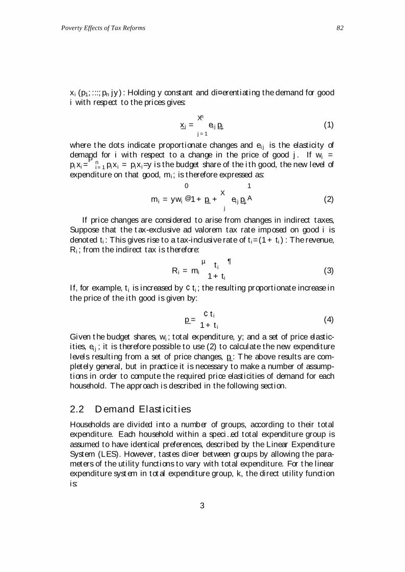
Poverty Effects of Tax Reforms 82
x i (p1; :::; pn jy ) : Holding y constant and di¤erent iat ing thedemand for goodi with respect to the prices gives:
_x i =nX
j = 1ei j _pj (1)
where t he dots indicate proport ionate changes and ei j is the elast ici ty ofdemand for i with respect to a change in the price of good j . If wi =pi xi =
P ni = 1 pix i = pix i=y is the budget share of the i th good, the new level of
expenditure on that good, mi ; is therefore expressed as:
mi = ywi
0
@1+ _pi +X
jei j _pj
1
A (2)
If price changes are considered to arise from changes in indirect taxes,Suppose that the t ax-exclusive ad valorem tax rate imposed on good i isdenoted ti : This gives rise to a tax-inclusive rate of t i=(1+ ti ) : The revenue,Ri ; from the indirect tax is therefore:
Ri = mi
µ t i
1+ ti
¶(3)
I f, for example, t i is increased by ¢ ti ; the result ing proport ionate increase inthe price of the ith good is given by:
_p =¢ t i
1+ t i(4)
Given t he budget shares, wi ; total expenditure, y; and a set of price elast ic-i t ies, ei j ; it is therefore possible to use (2) to calculate the new expenditurelevels result ing from a set of price changes, _pi : The above results are com-pletely general, but in pract ice it is necessary to make a number of assump-t ions in order to compute the required price elast icit ies of demand for eachhousehold. The approach is described in the following sect ion.
2.2 D emand Elast ici t iesHouseholds are divided into a number of groups, according to their totalexpenditure. Each household within a speci…ed total expenditure group isassumed to have ident ical preferences, described by the Linear ExpenditureSystem (LES). However, tastes di¤er between groups by allowing the para-meters of the ut i lity funct ions to vary with total expenditure. For t he l inearexpenditure syst em in tot al expenditure group, k, the direct ut i lity funct ionis:
3

Poverty Effects of Tax Reforms 83
U =nY
i= 1(xk ;i ¡ °k;i )
¯k ; i (5)
with 0 · ¯k;i · 1; °k;i is thecommitted consumption of good i; andP n
i = 1 ¯k;i =1: Each of theparameters, ¯i and ° i have an addit ional subscript , k; to allowthem to vary wit h yk .
For the LES, the own-price elast ici ty of demand for the ith good, ek ii ; intotal expenditure group k; is:
eki i =° i (1 ¡ ¯k;i )
xk ;i¡ 1 (6)
The cross-price elast icity, eki j , that is t he elast ici ty of demand for good i inresponse to a change in the price of good j ; in tot al expenditure group k; is:
eki j = ¡¯k;i °k;j
xk;j
Ãwk ;j
wk;i
!
(7)
where wk;i = pi xk;i =yk is the expenditure or budget share of t he ith good.The total expendit ure elast icity of good i ; ek ;i ; is:
ek;i =¯k;iypi xk;i
= ¯k;i =wk;i (8)
Households in the HES are thus divided into separate total expendituregroups, and within each group, k; averagebudget shares for each commodity,wk ;i ; arecomputed. For k = 1; :::K tot al expendituregroups, thisgivesrisetoa rectangular matrix, f wk;i g ; of budget shares, with K rows and n columns.Comparisons between adjacent expendit ure groups gives a matrix of totalexpenditure elast icit ies, using ek;i = 1 + _wk;i =_yk (where the dots actual lyindicate discrete changes from group k ¡ 1 to k).
The ek;i are then used to calculate the ¯k;i from (8) using k̄; i = wk;i ek;i :Given own-price elast icit ies of demand for each good at each income level,equat ion (6) can be used to give pi°k;i . The own- and cross-pr ice elast ici t iesare …rst obtained using a property of direct ly addit ive ut ility funct ions. Itcan be shown t hat:
ek ij = ¡ ek;i wk;j
Ã
1 +ek;j
»k
!
(9)
ek ii = ek;i
(1»k
¡ wk;i
Ã
1+ek;i
»k
! )
(10)
4
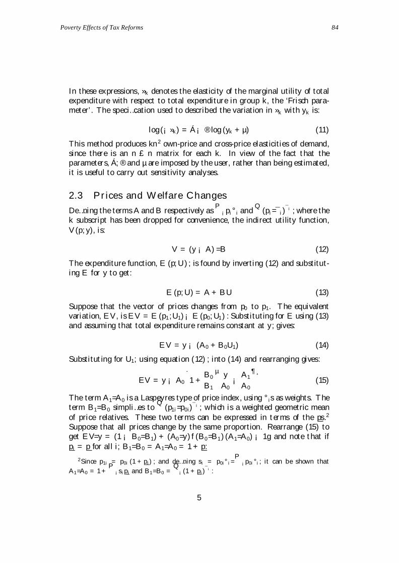
Poverty Effects of Tax Reforms 84
In these expressions, »k denotes the elast ici ty of the marginal ut ili ty of totalexpenditure with respect to total expenditure in group k, the ‘Frisch para-meter’ . The speci…cation used to described the variat ion in »k with yk is:
log(¡ »k ) = Á ¡ ®log (yk + µ) (11)
This method produces kn2 own-price and cross-price elast icit ies of demand,since there is an n £ n matrix for each k. In view of the fact t hat theparameters, Á; ®and µ are imposed by theuser, rather than being est imated,i t is useful to carry out sensit ivi ty analyses.
2.3 Pr ices and W elfare ChangesDe…ning the termsA and B respect ively as
Pi pi ° i and
Q(pi =̄ i )
¯i ; where thek subscript has been dropped for convenience, the indirect ut i lity funct ion,V (p; y), is:
V = (y ¡ A) =B (12)
The expenditure funct ion, E (p; U) ; is found by invert ing (12) and subst itut-ing E for y to get:
E (p; U) = A + B U (13)
Suppose that the vector of prices changes from p0 to p1. The equivalentvariat ion, E V, isE V = E (p1;U1) ¡ E (p0; U1) : Subst i tut ing for E using (13)and assuming that total expenditure remains constant at y; gives:
E V = y ¡ (A0 + B0U1) (14)
Subst i tut ing for U1; using equat ion (12) ; into (14) and rearranging gives:
EV = y ¡ A0
·1 +
B0
B1
µ yA0
¡A1
A0
¶ ¸(15)
The term A1=A0 isa Laspeyres typeof price index, using ° is as weights. Theterm B1=B0 simpli…es to
Q(p1i =p0i )
¯ i ; which is a weighted geometric meanof price relat ives. These two terms can be expressed in t erms of the _ps.2
Suppose that all pr ices change by the same proport ion. Rearrange (15) toget E V=y = (1 ¡ B0=B1) + (A0=y) f (B0=B1) (A1=A0) ¡ 1g and note t hat if_pi = _p for al l i ; B1=B0 = A1=A0 = 1+ _p:
2Since p1i = p0i (1 + _pi ) ; and de…ning si = p0i ° i =P
i p0i ° i ; it can be shown thatA1=A0 = 1+
Pi si _pi and B1=B0 =
Qi (1 + _pi )
¯ i :
5

Poverty Effects of Tax Reforms 85
2.4 Equivalent I ncomesEquivalent income is de…ned as the value of income, ye, which, at somereference set of prices, pr , gives t he same uti lity as the actual income level.In this context, income and tot al expenditure are treated as synonymous. Interms of t he indirect ut i lity funct ion, ye is therefore de…ned by V (pr ; ye) =V (p; y) : Using the expenditure funct ion gives:
ye = E (pr ; V (p;y)) (16)
For the linear expenditure system, this is found to be:
ye =X
ipr i ° i +
8<
:
Y
i
Ãpr i
pi
! ¯i9=
;
8<
: y¡X
jpj ° j
9=
; (17)
The e¤ect on welfare of a change in prices and income can be measuredin terms of a change in equivalent incomes, from y0e to y1e, where, as before,the indices 0 and 1 refer to pre- and post-change values respect ively. Animportant feat ure of equivalent income is that it ensures that alternat ivesituat ionsareevaluated usinga common set of referenceprices. If pre-changeprices are used as reference prices, so t hat pr i = p0i for all i ; the post-changeequivalent income is thevalueof actual incomeafter thechange less thevalueof the equivalent variat ion; that is, y1e = y1 ¡ E V.
3 T he DAW ES Suit e of Pr ograms3.0.1 Pr ogram: D AW ES_ M .EX E
This takes budget shares for a range of income (tot al expenditure) groupsand calculates compensat ing and equivalent variat ions in each group for aset of price changes.
INPUT : The following input …les are required
² SHARES: The …rst line gives the number of income groups used. Theremainder contains, for each income group, the budget shares for eachcommodity group. This is presented in two ‘blocks’, whereby the …rstblock gives the shares for the …rst 7 commodity groups, the secondblock gives the shares for the last 7 groups;
² EXPEND: this contains the midpoints of the expenditure groups;
² FRISCH: this contains one line giving the parameters of the funct ionlog(¡ »k ) = Á ¡ ®log(yk + µ): Give Á; ®; µ; fol lowed by the minimumabsolute Frisch value;
6

Poverty Effects of Tax Reforms 86
² PRICES: this cont ains the proport ionate price changes
3.0.2 Pr ogram: D AW ES_ Y .EX E
This is the same as DAWES_ M.EXE but instead of providing the welfarechanges for the midpoint s given in EXPEND, it uses a set of values (with$100 intervals). The same input …les are used with the addit ion of UPPER,which contains the upper limits of the income classes used.
3.0.3 Pr ogram: D AW ES_ R .EX E
In thecont ext of achangein theindirect tax structure, thisprogam calculatestheset of tax rates required to producea speci…ed revenue, where the revenue…gure may be taken from the output from running DAWES_ M.EXE for agiven set of tax rates.
This program uses the same input …les as used for DAWES_ M.FOR,except that instead of PRICES, the input …le INREV is required. Thiscontains:
t1; :::; t14 ini t ial ‘ t rial’ values used for tax ratesR required revenue (from running LESEV for di¤ taxes)c1; :::; c14 ci = 0 if the ith tax rate is not to be adjusted
ci = 1 if the ith tax rate can be adjusted
3.0.4 Pr ogram: D AW ES_ H .EX E
Thisuses information about the total expendit ureof each of a largenumber ofhouseholds, taken from theHES, and produces the distribut ion of equivalentincome following a speci…ed set of proport ional pr ice changes.
INPUT : the …les, SHARES, EXPEND, FRISCH, PRICES and UPPER,asdescribeabove, are required. In addit ion, the…leHEXP.DAT contains thetotal expenditure data for the households. The …rst line gives thenumber ofhouseholds; then simply l ist the expenditure values. The equivalent incomevalues are placed in the …le INLORZ, which can be used with t he followingprogram.
3.0.5 Pr ogram: G IN I .EX E
This uses INLORZ, generated by DAWES_ H.EXE, in order to calculategen-eralised Gini, G(v) ; and Atkinson, A (") ; inequali ty measuresand associatedabbreviated social welfare funct ion values.
INPUT : in addit ion to INLORZ, the …le INGIN contains one line giving" 1; "2 and ¢ "; the init ial, …nal and incremental value of inequali ty aversion
7

Poverty Effects of Tax Reforms 87
for use with the Atkinson measure. The values used for v are "1 + 1; and soon.
8