The Posterior Distribution. Bayesian Theory of Evolution!

The Posterior Distribution

Bayesian Theory of Evolution!

Interpretation of Posterior Distribution

The posterior distribution summarizes all that we know after we have considered the data. For a full Bayesian the posterior is everything!“once the posterior is calculated the task is accomplished”However, for us in the applied fields, the full posterior distribution is often too much to consider and we want to publish simpler summaries of the results, i.e., to summarize results in just a few numbers.We should be careful, since these point summaries (estimates) we make are reflect only part of posterior behaviour.Although this may look similar to the point summaries that we are used to from frequentist statistical analysis (e.g., estimators like averages and standard deviations), the interpretation as well as the procedures are different


The simplest summary of the posterior distribution is to take some average over it

For example, if the posterior distribution is on some quantity like N we can consider the posterior mean of N:

Or, we can consider the posterior median of N, which is the value N* such that

N E(N) NP(N | D)all N

*

0

2/1)|(N

DNP

Interpretation of Posterior DistributionThe mode is the maximum of the posterior:

0

0.0005

0.001

0.0015

0.002

0.0025

0 500 1000 1500 2000

Number of Fish

Pro

bab

ilit

y

Median679

Mean727

Mode600

)|(max*

* DNPNN

Bayes Risk

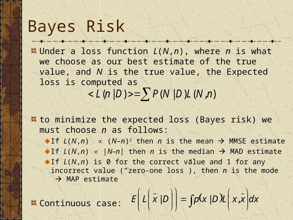
Under a loss function L(N,n), where n is what we choose as our best estimate of the true value, and N is the true value, the Expected loss is computed as

to minimize the expected loss (Bayes risk) we must choose n as follows:

If L(N,n) (N–n)2 then n is the mean MMSE estimate

If L(N,n) |N–n| then n is the median MAD estimate

If L(N,n) is 0 for the correct value and 1 for any incorrect value (“zero-one loss”), then n is the mode MAP estimate

Continuous case:

),()|()|( nNLDNPDnL

dxxxLDxpDxLE

__

,||


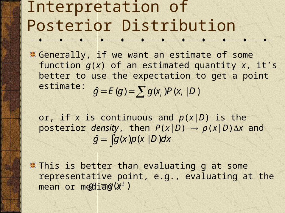
Generally, if we want an estimate of some function g(x) of an estimated quantity x, it’s better to use the expectation to get a point estimate:

or, if x is continuous and p(x|D) is the posterior density, then P(x|D) p(x|D)x and

This is better than evaluating g at some representative point, e.g., evaluating at the mean or median x+

ˆ g E(g) g(xi )P(xi | D)

ˆ g g(x)p(x | D)dx

g g(x )


If we have a Monte Carlo sample from the posterior distribution then we can calculate interesting things from the sample. For example, if our sample is {xi}, and we want to approximate the expectation of a function g(x) we simply calculate the average of g(xi) for the sample:

ˆ g E(g) 1

ng(xi )

Robustness

The posterior depends on the prior, and the prior is up to us. We may not be certain what prior reflects our true state of prior knowledge. In such cases we are led to ask what the dependence of the posterior on the prior isIf the posterior is insensitive to the prior, when the prior is varied over a range that is reasonable, believable and comprehensive, then we can be fairly confident of our results. This usually happens when there is a lot of data or very precise dataIf the posterior is sensitive to the prior, then this also tells us something important, namely, that we have not learned enough from the data to be confident of our result. (In such a case no statistical method is reliable…but only the Bayesian method gives you this explicit warning).

Robustness

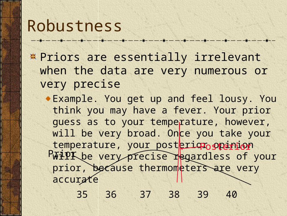
Priors are essentially irrelevant when the data are very numerous or very precise

Example. You get up and feel lousy. You think you may have a fever. Your prior guess as to your temperature, however, will be very broad. Once you take your temperature, your posterior opinion will be very precise regardless of your prior, because thermometers are very accurate

35 36 37 38 39 40

PriorPosterior

Robustness

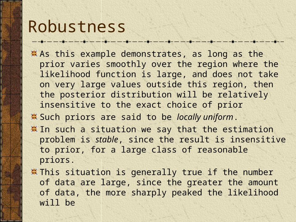
As this example demonstrates, as long as the prior varies smoothly over the region where the likelihood function is large, and does not take on very large values outside this region, then the posterior distribution will be relatively insensitive to the exact choice of prior

Such priors are said to be locally uniform.

In such a situation we say that the estimation problem is stable, since the result is insensitive to prior, for a large class of reasonable priors.

This situation is generally true if the number of data are large, since the greater the amount of data, the more sharply peaked the likelihood will be

Robustness

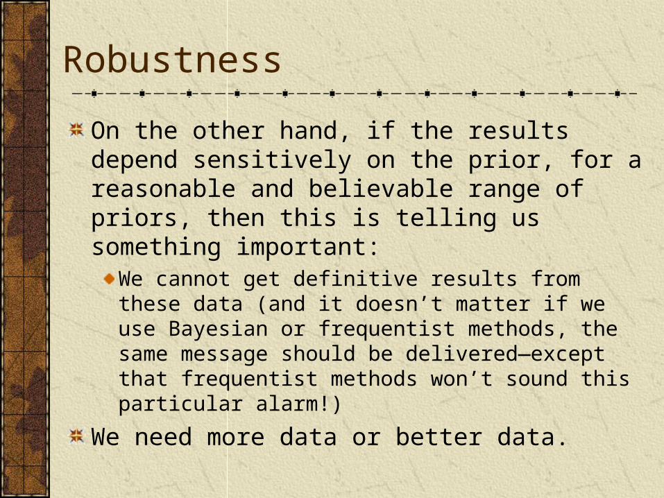
On the other hand, if the results depend sensitively on the prior, for a reasonable and believable range of priors, then this is telling us something important:

We cannot get definitive results from these data (and it doesn’t matter if we use Bayesian or frequentist methods, the same message should be delivered—except that frequentist methods won’t sound this particular alarm!)

We need more data or better data.

Inference on Continuous Parameters

A simple example is the Bernoulli trial: we have a biased coin. That is, we expect that if the coin is tossed then there is a probability b (not necessarily equal to 1/2) that it comes up heads. The bias b is unknown. How do we study this problem?

The probabilities are given by the following table:

Heads bTails 1-b


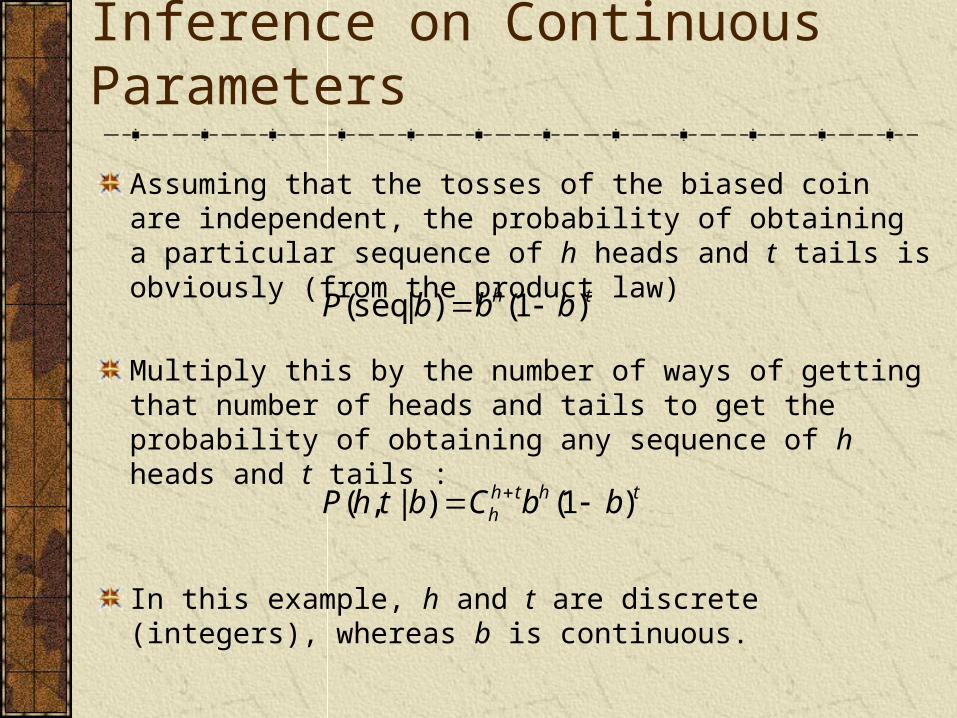
Assuming that the tosses of the biased coin are independent, the probability of obtaining a particular sequence of h heads and t tails is obviously (from the product law)

Multiply this by the number of ways of getting that number of heads and tails to get the probability of obtaining any sequence of h heads and t tails :

In this example, h and t are discrete (integers), whereas b is continuous.

P(seq | b) bh(1 b)t

P(h, t | b) Chh tbh (1 b)t


An interesting question is this: Given that we have observed h heads and t tails, what is the bias b of the coin (the probability that the coin will come up heads)?To answer this we have to follow the usual Bayesian procedure:

What are the states of nature?What is our prior on the states of nature?What is the likelihood?What is our posterior on the states of nature?How will we summarize the results?


What are the states of nature?In this case the states of nature are the possible values of b: real numbers in the interval [0,1]


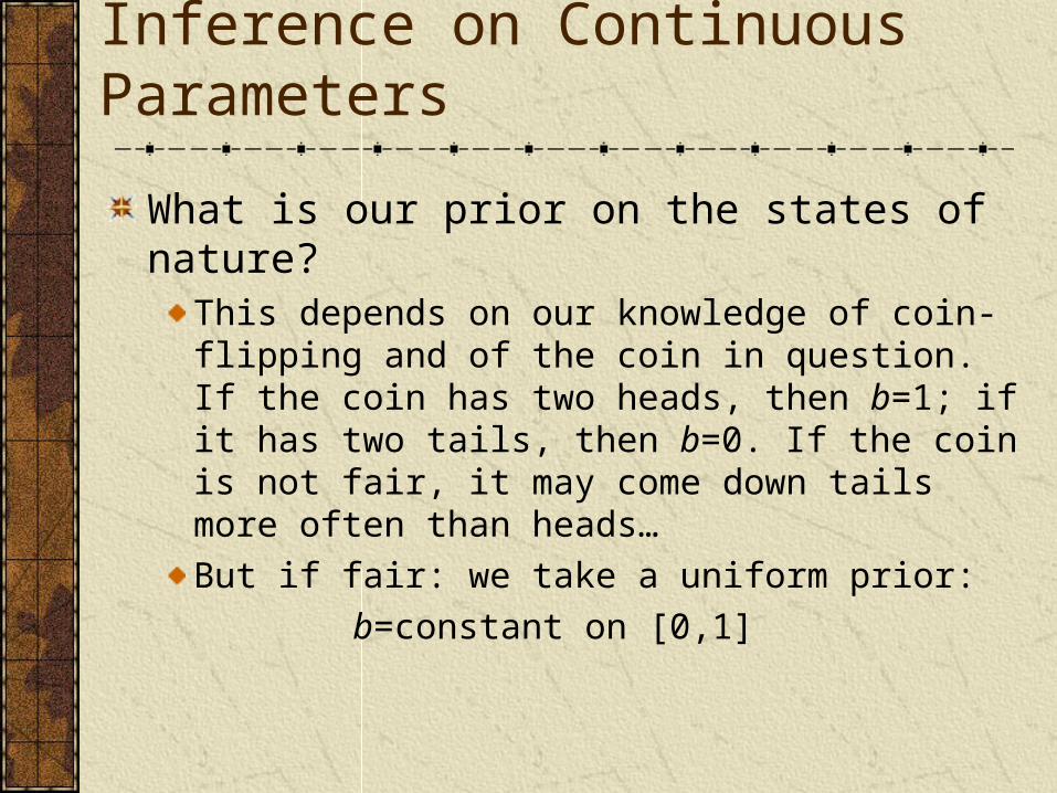
What is our prior on the states of nature?This depends on our knowledge of coin-flipping and of the coin in question. If the coin has two heads, then b=1; if it has two tails, then b=0. If the coin is not fair, it may come down tails more often than heads…

But if fair: we take a uniform prior:

b=constant on [0,1]


What is the likelihood?The likelihood is the probability of obtaining the results we got, given the state of nature under consideration. That is,

if we know the exact sequence, and

if we do not.

However, it doesn’t matter if we know the exact sequence or not! Since the data are independent and fixed, one likelihood is a constant multiple of the other, and the constant factor will cancel when we divide by the marginal likelihood. Order is irrelevant here.

P(seq | b) bh(1 b)t

P(h, t | b) Chh tbh (1 b)t


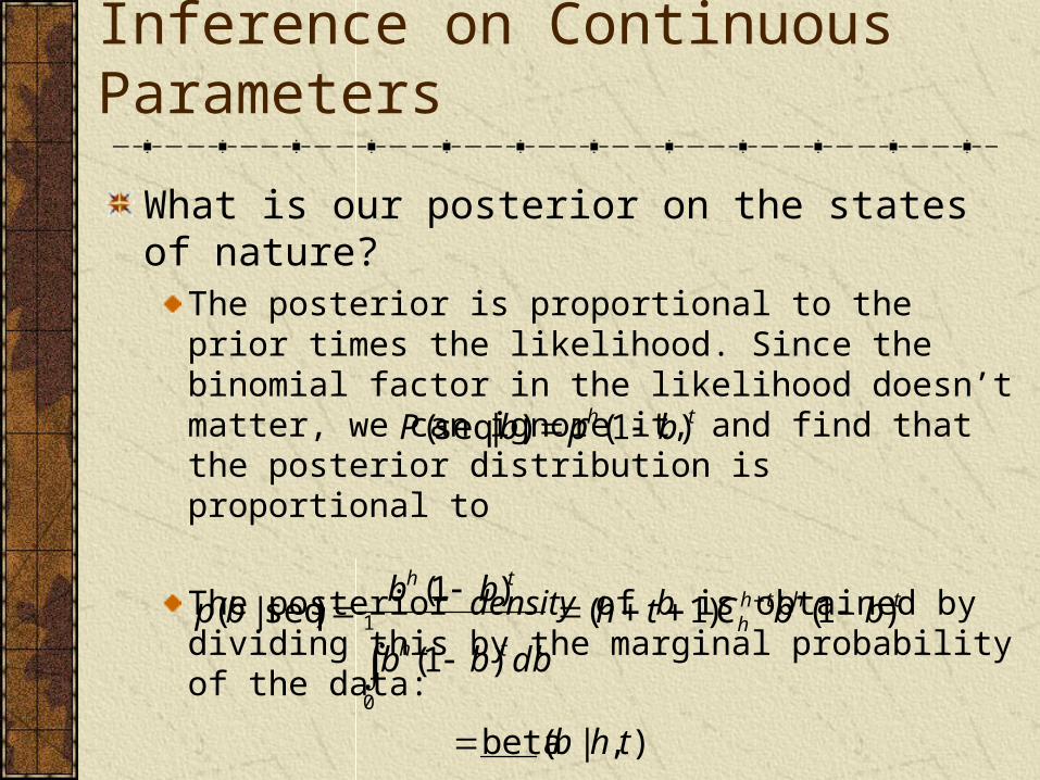
What is our posterior on the states of nature?The posterior is proportional to the prior times the likelihood. Since the binomial factor in the likelihood doesn’t matter, we can ignore it, and find that the posterior distribution is proportional to

The posterior density of b is obtained by dividing this by the marginal probability of the data:

P(seq | b) ph(1 b)t

p(b | seq) bh (1 b)t

bh(1 b)t db0

1

(h t 1)Ch

h tbh (1 b)t

beta(b | h,t)


How should we summarize the results?The Bayesian style would be to report the entire posterior distribution, or failing that, a selection of HDRsSometimes we want to summarize as a number or a number ± an errorExample: Bernoulli trials, h=20, t=9The mode of the likelihood function bh(1-b)t is at b*=h/(h+t)=0.69

This is the maximum a posteriori (MAP) estimator of b. It also is the maximum likelihood estimator (MLE) of b, since the prior is flat

Point Estimates

However,

This is similar to but not exactly equal to the mode. Both are reasonable and consistent with the data. As h+t they approach each other

E(b) b bh(1 b)t db

0

1

bh (1 b)t db0

1

h t 1

h t 2

Chht

Ch 1h t 1

h 1

h t 20.68

Point Estimates

The expectation is preferred to the MAP. Take for example, h=t=0. Then the MAP is h/(h+t) and is undefined, but the posterior mean is a reasonable (h+1)/(h+t+2)=1/2

This is obvious since there is no mode when h=t=0; the prior distribution is flat! However, there is still a mean.

Similarly, if h=1, t=0 then E(b)=2/3 whereas the MAP is 1/1=1, which seems overly biased towards 1 for such a small amount of data!

Again, with these data, the posterior distribution is a linear ramp from 0 to 1. Some probability exists for b<1, yet the MAP picks out the maximum at 1.

-10

0

10

20

30

40

50

60

0 0.2 0.4 0.6 0.8 1

Success Rate

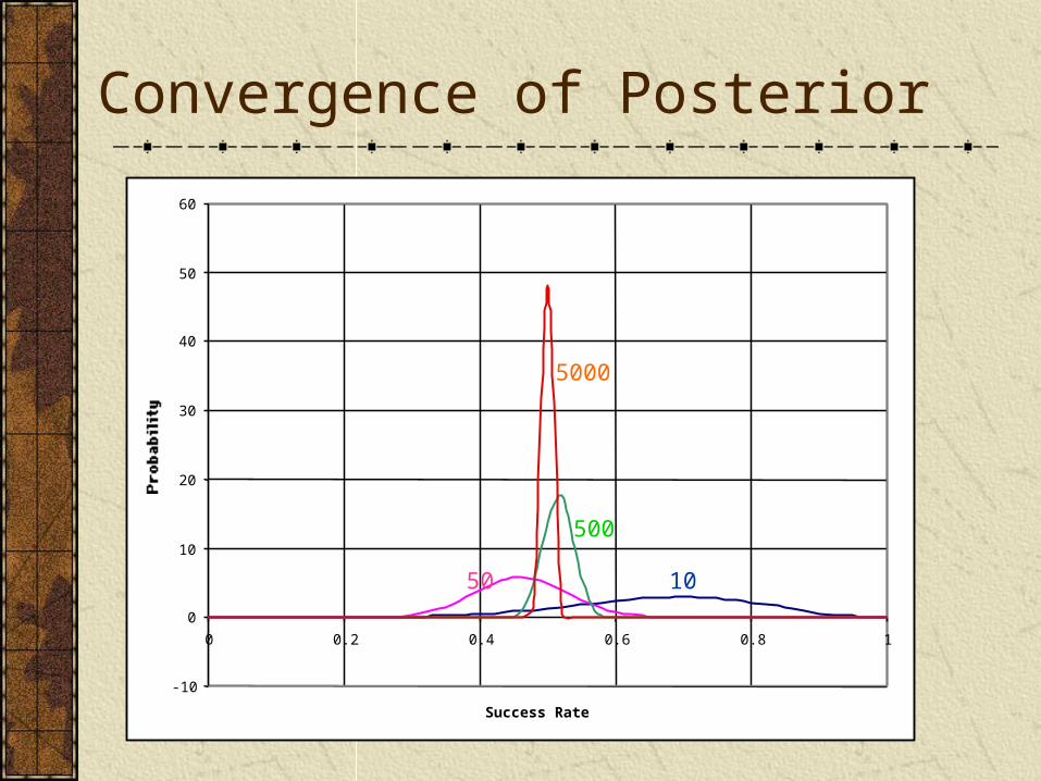
Convergence of Posterior

50

500

5000

10

Convergence of Posterior

The point is that as the data get more numerous, the likelihood function becomes more and more peaked near some particular value, and the prior is overwhelmed by the likelihood function.

In essence, the likelihood approaches a -function centered on the true value, as the number of data approaches infinity (which of course it never does in practice)

Nonflat Priors

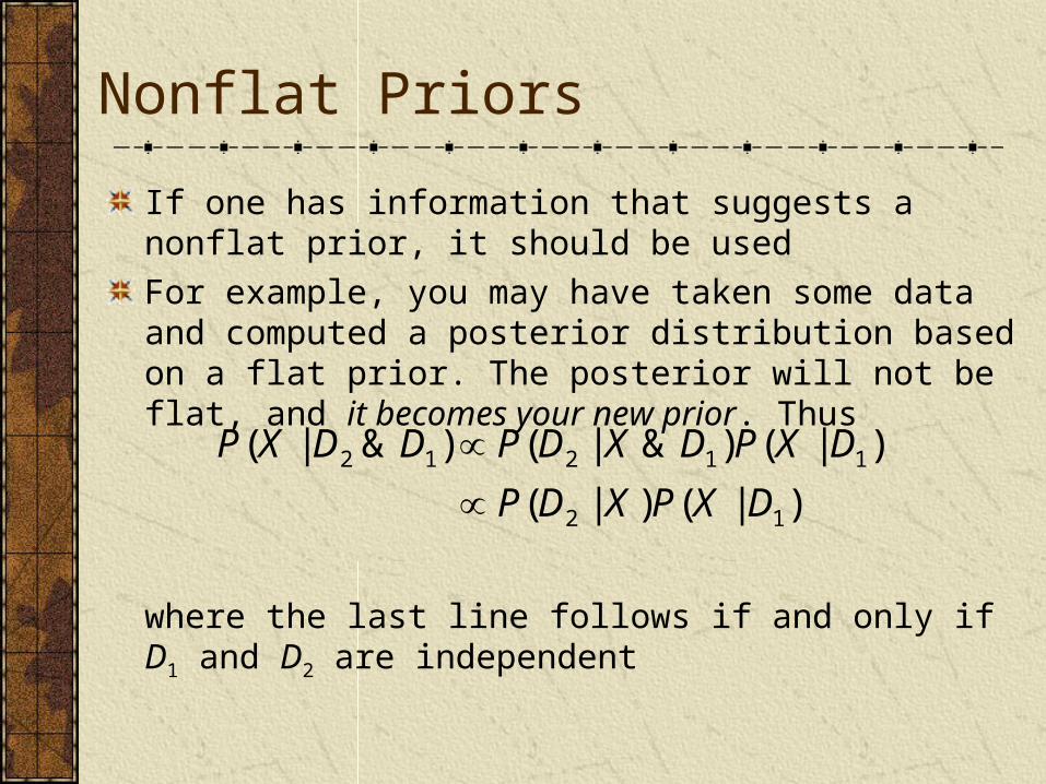
If one has information that suggests a nonflat prior, it should be used

For example, you may have taken some data and computed a posterior distribution based on a flat prior. The posterior will not be flat, and it becomes your new prior. Thus

where the last line follows if and only if D1 and D2 are independent

)|()|(

)|()&|()&|(

12

11212

DXPXDP

DXPDXDPDDXP

Nonflat Priors

For example, suppose we have Bernoulli trials and observe s successes (“heads”) and f failures (“tails”)On a flat prior, the posterior for the probability b of getting a success is

If we now observe t successes and g failures, with the above as prior, we get the posterior

which is the same result that we would have gotten had we considered all of the data simultaneously with a flat prior. This is a very general result. We can “chunk” the data in any way that is convenient for our analysis

beta(b | s, f ) bs (1 b) f

beta(b | s t, f g) bst (1 b) f g

Nonflat Priors

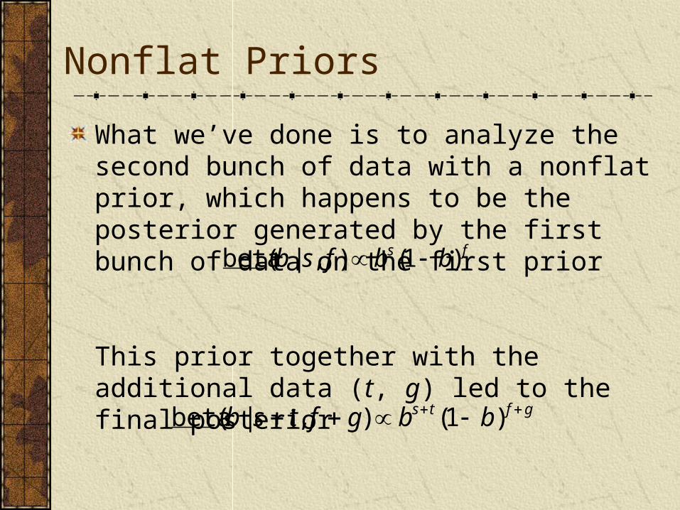
What we’ve done is to analyze the second bunch of data with a nonflat prior, which happens to be the posterior generated by the first bunch of data on the first prior

This prior together with the additional data (t, g) led to the final posterior

beta(b | s, f ) bs (1 b) f

beta(b | s t, f g) bst (1 b) f g

Nonflat Priors

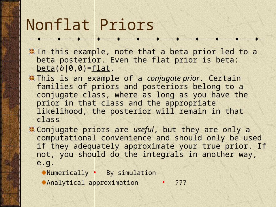
In this example, note that a beta prior led to a beta posterior. Even the flat prior is beta: beta(b|0,0)=flat.This is an example of a conjugate prior. Certain families of priors and posteriors belong to a conjugate class, where as long as you have the prior in that class and the appropriate likelihood, the posterior will remain in that classConjugate priors are useful, but they are only a computational convenience and should only be used if they adequately approximate your true prior. If not, you should do the integrals in another way, e.g.

Numerically • By simulation

Analytical approximation • ???

Sufficient Statistics

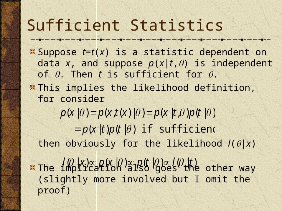
Suppose t=t(x) is a statistic dependent on data x, and suppose p(x|t,) is independent of . Then t is sufficient for .

This implies the likelihood definition, for consider

then obviously for the likelihood l(|x)

The implication also goes the other way (slightly more involved but I omit the proof)

p(x |) p(x,t(x) |) p(x | t,)p(t |)

p(x | t)p(t |) if sufficiency holds

l( | x) p(x |) p(t |) l( | t)

More on Sufficiency

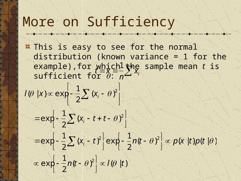
This is easy to see for the normal distribution (known variance = 1 for the example),for which the sample mean t is sufficient for :

l( | x) exp 12

(xi )2

exp 1

2(xi t t )2

exp 1

2(xi t)2

exp

1

2n(t )2

p(x | t) p(t | )

exp 12

n(t )2

l( | t)

t x 1

nxi

Example: Normal Distribution

With normally distributed data (mean m and variance 2), a sufficient statistic for m and is the set {x1,x2,…,xn}, and a minimal sufficient statistic is the pair

Show this, using the fact that the normal probability density is given by

x 1

nxi

i1

n

, Sxx2 (xi x )2

i 1

n

p(xi | m, 2 ) 1

2exp

(xi m)2

2 2

Example: Binomial distribution

Examples of sufficient statistics include one we have already seen: When flipping a coin, the numbers h and t of heads and tails, respectively, are a sufficient statistic, since the likelihood is proportional to ph(1–p)t.

The exact sequence of heads and tails is also a sufficient statistic; however it is not minimal (it contains more information than necessary to construct the likelihood)

Example: Cauchy Distribution

Another interesting example is inference on the Cauchy distribution, also known as the Student or t distribution with 1 degree of freedom.

This distribution is best known in statistics, but it arises naturally in physics and elsewhere

In physics, it is the same as the Lorentz line profile for a spectral line


It is also the response to an isotropic source of particles for a linear detector some distance away from the source

x

r1

P(detect at x) 1

1

1 (x x0 )2 1

r2

x0


The variance of the Cauchy distribution is infinite; this is easily shown

Prove this!

The mean is not well defined either (the integral is not uniformly convergent)...and this has unpleasant consequences

For example, the average of iid (identically and independently distributed) samples from a distribution is often held to approach a normal distribution, via the central limit theorem, as the sample gets large; however, the central limit theorem does not apply when the variance is infinite


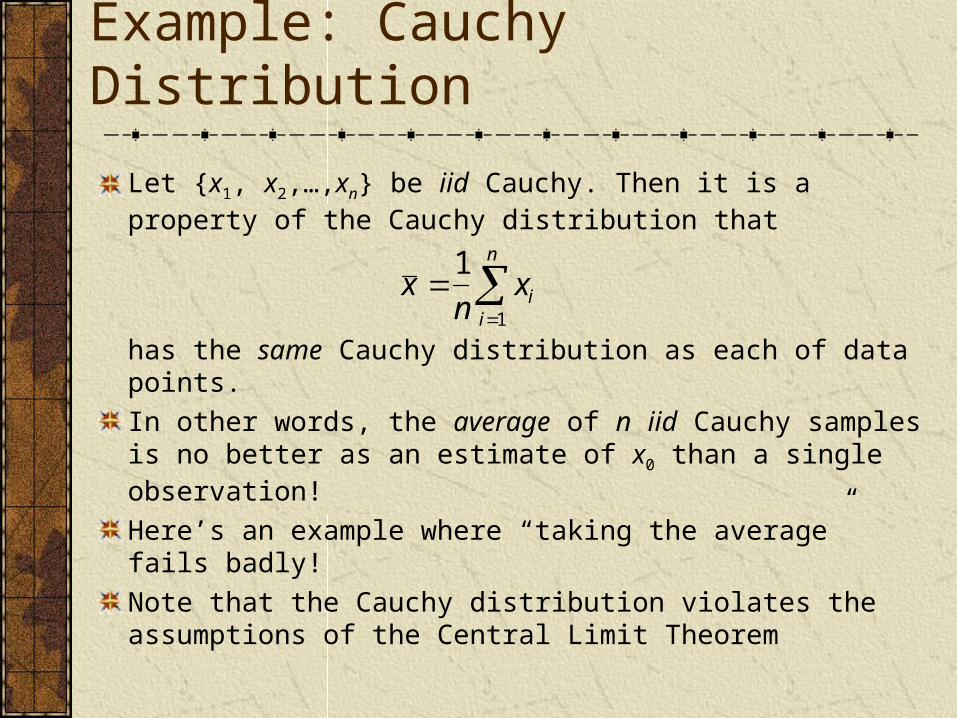
Let {x1, x2,…,xn} be iid Cauchy. Then it is a property of the Cauchy distribution that

has the same Cauchy distribution as each of data points.

In other words, the average of n iid Cauchy samples is no better as an estimate of x0 than a single observation!

Here’s an example where “taking the average” fails badly!

Note that the Cauchy distribution violates the assumptions of the Central Limit Theorem

x 1

nxi

i1

n


Bayesians always start with the likelihood function, which I will here augment with a parameter which measures the spread (not the variance!) of the distribution

The likelihood (for Cauchy) is a sufficient statistic for x0 and —but the sample mean (average) is not!

A statistic (any function of the data) is sufficient for parameters if you can construct the likelihood for from it; here the data {x1, x2,…,xn} are a sufficient statistic as, of course, is the likelihood—but the average is not! {x1, x2,…,xn} is a minimal sufficient statistic in the Cauchy case; no smaller set of numbers is sufficient

L(x0 |{x1,..., xn}) 1

( )n 1xi x0

2

1

i1

n

Consistency

Because of the property of the standard (i.e., =1) Cauchy distribution that we’ve discussed, no matter how much data we take, the average will never “settle down” to some limiting value. Thus, not only is the average not a sufficient statistic for x0, it is also not a consistent estimator of x0.

An estimator of a parameter is consistent if it converges in probability to the true value of the parameter in the limit as the number of observations Convergence in probability means that the probability that the estimates will converge to the true value is 1.

Bias

An estimator is biased if its expectation does not equal the true value of the parameter being estimated. For example, for Cauchy data the estimator of x0 is unbiased and inconsistent, whereas for normal data the estimator

of m is biased and consistent, and the estimator is unbiased and consistent. The estimator 1.1 (should one be crazy enough to use it) is biased and inconsistent

x

x n

n 1

x x

Issues relevant to Bayesian inference?

I mention these issues since they are frequently seen in frequentist statistics. They are not of much importance in Bayesian inference because

Bayesian inference always uses a sufficient statistic, the likelihood, so that is never an issue

We do not construct estimators as such; rather we look at posterior distributions and marginal distributions and posterior means, and questions of bias and consistency are not issues. The posterior distribution is well behaved under only mildly restrictive conditions (e.g., normalisability), and as the size of the sample it becomes narrower and more peaked about the true value(s) of the parameter(s)


Thus, inference on the Cauchy distribution is no different from any Bayesian inference:

Decide on a prior for x0 (and )

Use the likelihood function we have computed

Multiply the two

Compute the marginal likelihood

Divide to get the posterior distribution

Compute marginals and expectations as desired

The Posterior Distribution. Bayesian Theory of Evolution!

Documents

Transcript of The Posterior Distribution. Bayesian Theory of Evolution!