The Political Economy of the U.S. Mortgage Default · PDF fileThe Political Economy of the U.S...
51
NBER WORKING PAPER SERIES THE POLITICAL ECONOMY OF THE U.S. MORTGAGE DEFAULT CRISIS Atif Mian Amir Sufi Francesco Trebbi Working Paper 14468 http://www.nber.org/papers/w14468 NATIONAL BUREAU OF ECONOMIC RESEARCH 1050 Massachusetts Avenue Cambridge, MA 02138 November 2008 The authors would like to thank Alberto Alesina, Paul Beaudry, Matilde Bombardini, Patrick Francois, David Lucca, Don Morgan, Torsten Persson, Riccardo Puglisi, and Guido Tabellini for useful comments and discussion. We would also like to thank seminar participants at Bocconi University, Chicago GSB, the Federal Reserve Banks of Kansas City and New York, the University of Maryland, Princeton University, Stockholm University, and the World Bank for comments. We are grateful to the Initiative on Global Financial Markets at Chicago GSB for financial support. The views expressed herein are those of the author(s) and do not necessarily reflect the views of the National Bureau of Economic Research. NBER working papers are circulated for discussion and comment purposes. They have not been peer- reviewed or been subject to the review by the NBER Board of Directors that accompanies official NBER publications. © 2008 by Atif Mian, Amir Sufi, and Francesco Trebbi. All rights reserved. Short sections of text, not to exceed two paragraphs, may be quoted without explicit permission provided that full credit, including © notice, is given to the source.
Transcript of The Political Economy of the U.S. Mortgage Default · PDF fileThe Political Economy of the U.S...

NBER WORKING PAPER SERIES
THE POLITICAL ECONOMY OF THE U.S. MORTGAGE DEFAULT CRISIS
Atif MianAmir Sufi
Francesco Trebbi
Working Paper 14468http://www.nber.org/papers/w14468
NATIONAL BUREAU OF ECONOMIC RESEARCH1050 Massachusetts Avenue
Cambridge, MA 02138November 2008
The authors would like to thank Alberto Alesina, Paul Beaudry, Matilde Bombardini, Patrick Francois,David Lucca, Don Morgan, Torsten Persson, Riccardo Puglisi, and Guido Tabellini for useful commentsand discussion. We would also like to thank seminar participants at Bocconi University, Chicago GSB,the Federal Reserve Banks of Kansas City and New York, the University of Maryland, Princeton University,Stockholm University, and the World Bank for comments. We are grateful to the Initiative on GlobalFinancial Markets at Chicago GSB for financial support. The views expressed herein are those of theauthor(s) and do not necessarily reflect the views of the National Bureau of Economic Research.
NBER working papers are circulated for discussion and comment purposes. They have not been peer-reviewed or been subject to the review by the NBER Board of Directors that accompanies officialNBER publications.
© 2008 by Atif Mian, Amir Sufi, and Francesco Trebbi. All rights reserved. Short sections of text,not to exceed two paragraphs, may be quoted without explicit permission provided that full credit,including © notice, is given to the source.

The Political Economy of the U.S. Mortgage Default CrisisAtif Mian, Amir Sufi, and Francesco TrebbiNBER Working Paper No. 14468November 2008JEL No. D72,G21,L51
ABSTRACT
We examine the determinants of congressional voting behavior on two of the most significant piecesof federal legislation in U.S. economic history: the American Housing Rescue and Foreclosure PreventionAct of 2008 and the Emergency Economic Stabilization Act of 2008. We find evidence that constituentinterests and special interests influence voting patterns during the crisis. Representatives from districtsexperiencing an increase in mortgage default rates are significantly more likely to vote in favor ofthe AHRFPA. They are precise in responding only to mortgage related constituent defaults, and aresignificantly more sensitive to defaults of their own-party constituents. Increased campaign contributionsfrom the financial services industry is associated with a higher likelihood of voting in favor of theEESA, a bill which transfers wealth from tax payers to the financial services industry. We also examinethe trade-off between politician ideology and constituent and special interests, and find that conservativepoliticians are less responsive to constituent and special interest pressure. This latter finding suggeststhat politicians, through ideology, can commit against intervention even during severe crises.
Atif MianUniversity of ChicagoGraduate School of Business5807 South Woodlawn AvenueChicago, IL 60637and [email protected]
Amir SufiUniversity of ChicagoGraduate School of Business5807 South Woodlawn AvneueChicago, IL [email protected]
Francesco TrebbiGraduate School of BusinessUniversity of Chicago5807 South Woodlawn AvenueChicago, IL 60637and [email protected]

1 Introduction
The U.S. mortgage default crisis has led to two of the most signi�cant pieces of emergency federal
legislation in U.S. economic history. In July 2008, after several months of steep deterioration in the
mortgage market, the U.S. Congress passed the American Housing Rescue and Foreclosure Preven-
tion Act (�AHRFPA�), a bill that provides up to $300 billion in Federal Housing Administration
insurance for renegotiated mortgages and unlimited support for Freddie Mac and Fannie Mae.1
In October 2008, the U.S. federal government enacted the Emergency Economic Stabilization Act
(�EESA�) which enables the Treasury Department to recapitalize banks through direct purchase
of new equity and severely distressed mortgage backed securities up to $700 billion. These bills
have forced an increase in the national debt ceiling of over $1 trillion, and they guarantee signi�-
cant government intervention in the mortgage market and �nancial industry for years to come. By
any standard, the AHRFPA and the EESA represent congressional legislation of historic economic
relevance and magnitude.
This paper analyzes the decision making process of U.S. Congressional representatives voting
on these bills. Our analysis is important on two dimensions. First, it details the political de-
terminants of the government�s response to the most severe �nancial crisis in U.S. history since
the Great Depression. Second, and perhaps more importantly, the passage of these bills provides
a unique opportunity to answer long-standing questions in political economy. More speci�cally,
political scientists and economists have long argued that government policy toward the economy is
determined by the con�uence of three factors: political ideology, constituent interests, and special
interests (Stigler, (1971), Posner (1974), Peltzman (1976), Kau and Rubin, (1979, 1993)). Em-
pirically separating these factors and understanding the mechanisms through which they operate
remains di¢ cult. As we show below, circumstances related to the passage of the emergency bills
coupled with a unique data set enable us to make signi�cant progress on these questions.
A key advantage of the emergency bills - relative to a substantial majority of existing congres-
sional voting studies - is that winners and losers are well speci�ed (Peltzman, (1984)). While both
bills con�ict with the fundamental conservative principle of limited intervention in private markets,
they each have speci�c �winners� that can be identi�ed empirically. The AHRFPA provides an
expected net transfer to households that are in (or near) default on their mortgages, while the
1The act is also known as the Housing and Economic Recovery Act of 2008 and the speci�c provision to provide
FHA insurance is the Hope for Homeowners program.
2

EESA provides an expected net transfer (at least in the short run) to the �nancial industry. We
refer to the former as �constituent interests�and latter as �special interests�in our analysis.
We utilize a unique data set that allows us to precisely measure these constituent and special
interests. The data set includes zip code level information on consumer credit defaults which we
use to construct the mortgage default rate at the congressional district level. In addition, the level
of geographical disaggregation in the data allows us to separately construct the default rate for
Republican and Democratic voters in a constituency. Our data set also includes information on the
average campaign contributions that a representative receives over a congressional cycle from the
�nancial industry.
We begin with an analysis of politician voting patterns on the AHRFPA. At its core, the bill
presents a con�ict between conservative ideology and constituent interests of defaulting mortgage
debtors. Separating the e¤ects of politician ideology from constituent interests has proven di¢ cult
in previous empirical studies because legislators with a track record of voting conservatively also
represent districts where constituent interests are naturally aligned with the conservative agenda
(Peltzman (1984) and (1985), Grier and Munger (1991), Poole and Rosenthal (1997), Levitt (1996)).
However, a unique advantage of the AHRFPA is that the shock to mortgage defaults that precedes
the bill is completely orthogonal to ideology.2 We therefore have a natural experiment to empirically
separate the in�uence of ideology versus constituent interests.
We �nd strong evidence that constituent interests a¤ect a politician�s voting choice. Represen-
tatives from high mortgage default districts are more likely to vote in favor of the AHRFPA, and
this result is not driven by ideological preferences or politician �type.�When we decompose the
2007 year end default rate into the 2005 year end default rate and the change in default rate from
2005 to 2007, we �nd that politicians only respond to the change in the mortgage default rate. Since
ideological preferences are �xed in the short run, this result implies that representatives respond
directly to time-varying constituent interests. Our preferred estimate suggests that a one standard
deviation increase in mortgage default rates in 2007 leads to a 12:6 percentage point increase in
the likelihood of voting for the AHRFPA. The �nding contradicts a purely ideological approach
to political representation (Bernstein (1989), Poole and Rosenthal (1996), Lee, Moretti and Butler
(2004)).
2This is true within the set of Republican districts, which is the relevant set since almost all Democrats voted in
favor of AHRFPA.
3

We provide several additional insights into the mechanisms through which constituent interests
a¤ect representatives� voting patterns. We �nd that representatives are remarkably precise in
responding to constituent interests. Since the mortgage bill has no impact on voters with credit
card or auto defaults, a representative should not change his voting behavior when the percentage
of non-mortgage related defaults changes. Despite the strong correlation of non-mortgage and
mortgage defaults in the data, we �nd that politicians react only to mortgage defaults while ignoring
non-mortgage defaults.
Employing zip code level information, we also separate the overall mortgage default rate into
the mortgage default rate experienced by Republican and Democratic voters within a congressional
district, and we show that politicians do not respond equally to all constituents. Instead, repre-
sentatives respond primarily to their own voting bloc. These results provide support to the �dual
constituency� hypothesis that legislators respond more strongly to their own supporters within
their electorate (Fiorina (1974)). To the best of our knowledge, ours is the �rst work that provides
evidence of the geographical precision with which politicians respond to their constituency.
If representatives are responding to constituent interests due to electoral pressure, then the
e¤ect of constituent interest on voting behavior should be stronger in more competitive districts.
Consistent with this prediction, we �nd that representatives are more likely to respond to an increase
in their constituent mortgage default rate by voting in favor of the AHRFPA if their election is
closely contested or if their district lies in a presidential swing state.
In our examination of politician voting patterns on the EESA, we �nd that a strong predictor
of voting behavior is the amount of campaign contributions from the �nancial services industry.
This �nding is consistent with anecdotal evidence suggesting that the �nancial industry lobbied
heavily to shape the EESA and get it passed. However, we are cautious in our interpretation of
this result. As Stratmann (2002, p. 346) emphasizes, �if interest groups contribute to legislators
who support them anyway, a signi�cant correlation between money and votes does not justify
the conclusion that money buys votes. In this case the positive correlation arises because the
same underlying factors that cause a group to contribute to a legislator also cause a legislator to
vote in the group�s interest�.3 While this is a genuine concern, the signi�cance of the impact of
3Di¤erent strands of theoretical work on special interests are present in the literature with a Political Science
strand focusing mostly on informational asymmetries (Austen-Smith (1987) and (1995)) and an Economic literature
focusing on policy buying following Grossman and Helpman (1994). The "policy buying" approach has produced
important empirical analysis in particular with regard to trade policy (Goldberg amd Maggi (1999), Gawande and
4

�nancial service campaign contributions on voting patterns for the EESA is remarkably robust to
the inclusion of many reasonable proxies for the �underlying factors� such as politician ideology,
district demographics, the fraction of constituents working for the �nancial industry, and whether
the representative serves on the �nancial committee. The magnitude of our estimate implies that a
one standard deviation increase in log campaign contributions from the �nancial services industry
is associated with a 10 percentage point increase in the likelihood of a politician voting for the bill.
While the two bills di¤ered in the identity of their direct bene�ciaries, they shared the com-
mon characteristic that they both con�icted with the fundamental conservative ideology of limited
government intervention. This friction was apparent in the debates leading up to the two votes as
ideologically conservative Republicans strongly objected to the bills on philosophical grounds. Not
surprisingly, we �nd that conservative ideology strongly predicts votes against the two bills.
In our analysis of ideology versus constituent and special interests, our ability to separate the
e¤ects of each allows us to estimate the �price�of the trade-o¤ between ideological and economic
voting incentives. While heightened constituent and special interests push politicians to vote in
favor of massive government intervention, we �nd that conservative politicians with ideological op-
position to the legislation are signi�cantly less responsive to such heightened interests. In other
words, the e¤ect of mortgage default rates on the AHRFPA vote and the e¤ect of campaign contri-
butions on the EESA vote are signi�cantly weaker among ideologically conservative representatives.
These results highlight the importance of political ideology as a partial commitment device against
government intervention: Ideologically conservative politicians are less responsive to constituent
and special interests even in the midst of a major �nancial crisis.
To our knowledge, this latter result is a novel documentation of the commitment value of
ideological preferences in resisting constituent and special interest pressures.4 This is an important
point, given that the ability to partially commit against ex post intervention is an important aspect
of the pricing of systematic risk as it relates to extreme �nancial crisis situations. This �nding
is related to a number of theoretical papers that rationalize the existence of di¤erent political
Bandyopadhyay (2000)). For a complete review of the empirical works on campaign contribution in�uence and its
consequences see Grossman and Helpman (2001), Stratmann (1991), and Stratmann (2005). For a critical review of
the rationality of political investment see Ansolabehere, de Figueiredo, and Snyder (2003), Bombardini and Trebbi
(2008a, 2008b).4An interesting work on the rationality of ideology as a form of committment against shirking is Dougan and
Munger (1989).
5

institutions - such as democracy, party politics, majority rules - as useful commitment devices (for
example, Acemoglu and Robinson (2001), Acemoglu, Johnson and Robinson (2005) and Bolton
and Rosenthal (2002)). It is also related to the literature on the political economy of �nancial
markets (Perotti and von Thadden (2006), Kroszner and Strahan (1999), Kroszner and Rajan
(1994), Kroszner (1991), and Khwaja and Mian (2004)). Our analysis of special interests is most
closely related to empirical political economy studies of the savings and loan debacle in the 1980s
(Romer and Weingast (1991)) and consumer bankruptcy reform (Nunez and Rosenthal (2004)).
The rest of our analysis proceeds as follows. The next section provides background on the
AHRFPA and the EESA, and describes how these bills were perceived by constituent and special
interests. Section 3 presents the data and summary statistics. Section 4 presents the empirical
model. The results on the AHRFPA appear in Section 5, while the ESSA is studied in Section
6. Further implications on the interaction of ideology and constituent interests of congressmen are
addressed in Section 7. The last section concludes.
2 The Legislative Response to the Mortgage Default Crisis
In this section, we describe the two pieces of legislation that are central to our analysis of the
mortgage crisis. We also describe how these bills were perceived by constituents and special interests
at the time of passage.
Before describing the details of the bills, it is important to emphasize the magnitude of the
mortgage default crisis and its e¤ects on the economy. From 2005 to 2007, Mian and Su� (2008)
show that the aggregate default rate on mortgages more than doubled. According to the S&P/Case
Shiller home price indices, home prices have declined by 20% since the peak in 2006. The U.S.
Department of Treasury was forced to nationalize the mortgage giants Freddie Mac and Fannie
Mae in September 2008 given their enormous losses on subprime mortgage backed securities. Some
of the world�s largest �nancial institutions, including Bear Stearns, AIG, Lehman Brothers, and
Washington Mutual, have failed or been acquired directly because of the plummeting value of
subprime and prime mortgage backed securities. It is in this environment that the U.S. Congress
has conducted a massive intervention in �nancial markets through the AHRFPA and the EESA.
6

2.1 The American Housing Rescue and Foreclosure Prevention Act of 2008
The initial U.S. Congressional response to the mortgage default crisis evolved between the summer
of 2007 and the summer of 2008, leading to the signing of the American Housing Rescue and
Foreclosure Prevention Act (AHRFPA) on July 30, 2008 by President Bush.5 The �nal version
of the AHRFPA included a number of provisions meant to aid the ailing housing sector. The act
gave the U.S. Federal Government, through the Federal Housing Administration, the ability to
insure $300 billion of re�nanced mortgages. Such insurance was provided for mortgage lenders that
voluntarily agreed to reduce mortgage principal and delinquency fees.6
The AHRFPA also increased the Treasury�s authority under existing lines of credit to Freddie
Mac, Fannie Mae, and the Federal Home Loan Banks for 18 months, giving Treasury standby
authority to buy stock or debt in those companies. The amount of the line of credit was unlimited
during these 18 months.7 In addition, the act increased FHA loan limits and provided tax breaks
for �rst-time home buyers. Finally, the act called for a regulatory overhaul of the O¢ ce of Federal
Housing Enterprise Oversight (OFHEO) by establishing the Federal Housing Finance Agency, which
is charged with broad supervisory and regulatory powers over the operations, activities, corporate
governance, safety and soundness, and mission of the Government Sponsored Enterprises (GSEs).
Overall, at the time of passage, the AHRFPA represented one of the most dramatic government
interventions in the housing sector in recent history. The New York Times (July 24th, 2008)
reported that �[the legislation] would rank in importance with the creation of the Home Owners�
Loan Corporation to prevent foreclosures in the 1930s as part of the New Deal, and the legislation
in 1989 responding to the savings and loan crisis.�8 A quote from a Wall Street Journal article
(July 24th, 2008) argued that � ... this is the most important piece of housing legislation to come
along in a generation.�As Paletta and Hagerty (2008) noted, �as a result of the bill, Congress will
raise the national debt ceiling to $10:6 trillion from $9:8 trillion.�
In discussing how constituent and special interests perceived this legislation, it is important to
5The following information comes from a document entitled "H.R. 3221: Detailed Summary" available at
http://�nancialservices.house.gov/detailed_summary_of_hr_3221.pdf. See also Herszenhorn (2008), Montgomery
(2008), and Paletta and Hagerty (2008). This act is also known as the Housing and Economic Recovery Act of 2008.6This part of the act is now known as the Hope for Homeowners program.7This line of credit to Fannie Mae and Freddie Mac became obselete in September 2008 when the U.S. Department
of Treasury took over the institutions.8For analysis of the farm foreclosure moratoria in the 1920�s and 1930�s see Alston (1984) and Alston and Rucker
and Alston (1987). For the S&L crisis, Romer and Weingast (1991).
7

emphasize that politician voting patterns were in�uenced by the perceptions of these interests at the
time of passage. In terms of the perceived bene�ciaries of the legislation, the primary component of
the bill, the FHA insurance for renegotiated mortgages, represented a transfer from tax payers to
the lenders and borrowers that renegotiate mortgages. Under the legislation, the renegotiation of
any mortgage is voluntary, which implies that neither lenders nor borrowers could be made worse
o¤ directly from the bill. There is, however, some evidence that mortgage lenders faced implicit
pressure to agree to write down principal in order to initiate renegotiations. For example, on the
day the bill was passed, Representative Barney Frank (D-MA), chairman of the House Financial
Services Committee, was quoted in the New York Times as follows: �Many of these institutions
know this is coming. I hope they will be able to take advantage of it right away.� And in the
Washington Post, Frank is quoted as follows: �I would be very disappointed if, having helped us
formulate this, they don�t take advantage of it.�Overall, the primary bene�ciaries of the legislation
were households either in default or close to default on mortgage payments. Mortgage lenders were
also bene�ciaries, but there may have been implicit Congressional pressure that would reduce the
bene�ts if mortgage lenders were forced to renegotiate mortgages at a loss.
Our main focus in the empirical analysis below is the vote on the �nal passage of this bill held
on July 26th, 2008.9 However, there was also an amendment vote on May 8th, 2008; the focus of
this previous vote was the $300 billion insurance program, as Freddie Mac and Fannie Mae had
yet to experience sharp losses that required government intervention.10 In speci�cations below, we
exploit the fact that some politicians switched votes to help understand the determinants of voting
behavior on the �nal version of the bill.9Roll call 519: "Concur in Senate Amendment with House Amendment: H R 3221 Foreclosure Prevention Act of
2008".10Roll call 301: "On Agreeing to the Senate Amendment with Amendment No. 1: H R 3221 Foreclosure Prevention
Act of 2008". This vote is considered by many the �rst crucial roll call in the political economy of the crisis and
was characterized by strong opposition (and a veto threat) by the executive branch. The Wall Street Journal (May
9, 2008) refers to the vote as follows: "The House voted 266-154 in favor of the centerpiece of the legislation �$300
billion in federal loan guarantees �despite a White House veto threat." In particular, "The heart of the legislation
is a program to help struggling homeowners by providing them with new mortgages backed by the Federal Housing
Administration. The guarantees would be provided if lenders agree to reduce the principal of a borrower�s existing
mortgage."
8

2.2 The Emergency Economic Stabilization Act of 2008
Beginning in the second week of September 2008, a series of events indicated that the U.S. �nancial
sector was in the midst of a severe crisis. While the lack of capital in the banking industry had
been a problem since August of 2007, more troublesome patterns emerged with the nationalization
of Fannie Mae and Freddie Mac and the distress at Lehman Brothers during the week of September
8th, 2008. On Monday, September 15th, Lehman Brothers submitted the largest bankruptcy �ling
in history. On Tuesday, September 16th, the US government nationalized the American Interna-
tional Group (AIG) after the insurance �rm experienced sharp losses and potential downgrades
related to the writing of credit default swaps. On Wednesday, September 17th, a few large money
market funds �broke the buck,�which e¤ectively meant losses on deposits that were supposed to
be close to riskless. In the midst of the �nancial market turmoil, on Friday, September 19th, initial
news reports suggested that �the federal government is working on a sweeping series of program
that would represent perhaps the biggest intervention in �nancial markets since the 1930s�(Wall
Street Journal, September 19th).
The EESA (2008) passed the U.S. House of Representatives on Friday, October 3rd. The
hallmark of the legislation was authorization for the U.S. Department of Treasury to buy up to $700
billion of �mortgages and other assets that are clogging the balance sheets of �nancial institutions
...� (Dodd (2008)). While the original intention of the bill was for the Treasury to buy severely
distressed subprime mortgage backed securities, more recent interpretations suggest that the act
can be used by Treasury to inject capital directly into banks through an equity investment. The
bill also included up to $150 billion of unrelated tax breaks for individuals and businesses, and an
increase in FDIC insurance for depositors from $100; 000 to $250; 000.
How was this bill perceived by constituents and special interests? At least in the short run,
it is clear that the legislation represented a large wealth transfer from U.S. tax payers to the
�nancial services industry. At the time of this writing, the Treasury has yet to purchase assets or
equity from �nancial institutions. But if the legislation is to help resolve the lack of capital in the
banking industry, it will most likely involve purchasing distressed assets and equity from �nancial
institutions at values above what the private market is willing to pay. For this reason, the most
direct bene�ciary of the legislation was the �nancial services industry.
Our main focus in the empirical analysis is the vote in the U.S. House of Representatives on
9

this bill on October 3rd, 2008.11 There was also a vote on Monday, September 29th, 2008.12 In the
initial vote, the House rejected the bill, inducing one of the largest single day stock market losses in
history. The October 3rd bill was di¤erent in two main respects: �rst, it called on the FDIC to lift
protection from $100; 000 to $250; 000 for individual depositors. Second, it included the additional
tax breaks mentioned above. While our primary focus is on the October 3rd vote, we also examine
the characteristics of 58 legislators that voted against the September 29th bill and for the October
3rd bill.
3 Data and Summary Statistics
3.1 Data
Our analysis focuses on the determinants of House voting patterns on the AHRFPA and the EESA.
We focus on House votes given the additional geographic variation that comes from more precise
measures of constituent characteristics at the Congressional district, as opposed to state, level.
We utilize four main sets of data: consumer credit data, congressional electoral and voting data,
campaign contribution data, and voter registration data. Data on consumer debt outstanding
and delinquency rates are from Equifax Predictive Services. Equifax collects these data from
consumer credit reports, and aggregates the information at the zip code level. The availability of
disaggregated geographical data on defaults is a major advantage of our analysis, as it allows us
to measure constituent interests as they relate to the default crisis. Furthermore, the availability
of zip code level default data allows us to construct measures of a politician�s particular voting
bloc within the congressional district. The Equifax data are available at an annual frequency from
1991 to 1997, and at a quarterly frequency from 1998 through the fourth quarter of 2007.13 In the
following analysis, we de�ne default amounts as any amount that is 30 days or more delinquent.
The majority of our analysis focuses on mortgage default rates, but we also examine home equity
and non-housing consumer debt default rates in some of the results. In order to aggregate zip code
11Roll call vote 681 on "Motion to concur in Senate Amendment" on H.R. 1424 "Emergency Economic Stabilization
Act of 2008"12Roll call vote 674 on "On Concurring in Senate Amendment with an Amendment" on H.R. 3997 "To amend the
Internal Revenue Code of 1986 to provide earnings assistance and tax relief to members of the uniformed services,
volunteer �re�ghters, and Peace Corps volunteers, and for other purposes"13See Mian and Su� (2008) for further details on the Equifax data.
10

level data to the congressional district level, we utilize the MABLE-Geocorr software.14
Our second main data set covers congressional district electoral and voting behavior. These
data include party a¢ liation, vote margins in the November 2006 midterm elections, committee
assignments of the representatives from the district (Stewart and Woon (2008)), and the DW-
Nominate representative ideology scores which are increasing in conservatism (Poole and Rosenthal
(1985), (1997)).15
Our third main data set covers campaign contributions by special interest groups. We obtain
campaign contributions data from the Center for Responsive Politics (CRP), a nonpartisan and
nonpro�t organization that directly collects the information from the Federal Election Commission
political contributions reports.16 The advantage of the CRP data is that it covers contributions from
Political Action Committees (PACs, the main channel for �rms�political activity) and individual
contributions (above $200) sorted on the basis of the contributor�s employer. This allows for a
comprehensive measurement of the overall contributions of a speci�c industry. Our main industry
of interest is the Finance, Insurance, & Real Estate industry. The top four contributors from this
industry in the 2008 election cycle are Goldman Sachs ($4:5 million), Citigroup ($3:7 million), JP
Morgan Chase & Co ($3:3 million), and Morgan Stanley ($3:1 million).
Our fourth main data set has zip code level voter party a¢ liation information. This information
is available for 38 out of the 50 states, which cover 84% of U.S. Congressional Districts. For each
zip code, this data set records the fraction of voters belonging to the Republican and Democratic
party. Party a¢ liation of a voter is determined by the party with which she registers in 32 of the
38 states. In the remaining 6 states, party a¢ liation is determined by the party primary in which
a voter participates. The data are recorded as of 2007 for 32 states, 2006 for 4 states, and 2004 for
2 states. The data are provided by the political technology �rm Aristotle.17 Party a¢ liation data
allow us to weight zip code level default rates using the fraction of voters that are a¢ liated with
the Republican or Democratic party.
14Supported by the Missouri Census Data Center. Zip codes are 5-digit ZIP (ZCTA-ZIP Census Tab. Area 2000)
and matched to congressional districts. All the aggregates are population weighted sums.15Within the political science literature DW-nominate is one of the most popular proxies for ideology. In extreme
synthesis, the DW-Nominate score is an estimated ideological position based on the legislator�s past roll call voting
records within a random utility choice model.16See http://www.opensecrets.org and http://www.fec.gov/disclosure.shtml17We are extremely grateful to Matthew Gentzkow and Jesse Shapiro for sharing these data with us.
11

3.2 Summary Statistics
Table 1 presents summary statistics. The variables are split into �ve categories: measures of
constituent interests, measures of special interests, a measure of ideology, other political variables,
and census demographics. Districts are separated by the party a¢ liation of the representative in
the 110th Congress (2007-2008).
Our main proxy for constituent support for the AHRFPA of 2008 is the mortgage default rate
as of the end of 2007. While mortgage default rates for Democratic districts are higher than for
Republican districts in both 2005 and 2007, both experience a sharp increase in default rates over
these two years. For Republican districts, the increase in the mortgage default rate from 2005
to 2007 (2:2%) is equivalent to almost two standard deviations in the mortgage default level as
of 2005 (1:2%). The registered Republican and Democratic mortgage default rate is constructed
using the zip code level information on defaults and voter registration. The registered Republican
(Democratic) default rate is constructed as the population weighted sum of default rates across
zip codes where the weights are given by the fraction of registered Republicans (Democrats) in the
zip code. We also construct the �home default rate� by aggregating home equity defaults with
mortgage defaults, and the combined variable closely mirrors the mortgage default rate. Table
1 also includes information on the non-home default rate, which includes defaults on credit card
debt, auto debt, consumer loans, and student loans. We make use of this variable for falsi�cation
exercises.
Measures of constituent support for the EESA of 2008 include the fraction of the workforce
in a congressional district that is employed by the �nancial services industry and the fraction of
households with annual household income above $200; 000. In addition to the mortgage default
rate, these variables measure constituent support for the EESA, given that the bill represents a
transfer of wealth from tax payers to the �nancial services industry and those holding their assets.
Our primary measure of special interest support for the EESA is campaign contributions made
by the �nancial services industry, de�ned in the Center for Responsive Politics data as donations
from the Finance, Insurance and Real Estate industry. The statistics in Table 1 represent the
average campaign contribution per congressional term by the �nancial services industry since 1993
(103rd congress) for a given representative in the 110th congress. The mean for Republicans
and Democrats is about $142; 000 and $112; 000, respectively. In terms of politician�s ideology,
the DW nominate score, which is increasing in conservatism of the representative, is signi�cantly
12

lower for Democratic districts than for Republican districts. Table 1 also lists summary statistics
for political and census demographic control variables. Table A1 in the appendix shows the full
frequency distribution for the key right hand side variables in our analysis.
4 Empirical Model
4.1 Baseline
We derive and estimate a reduced-form model that examines the determinants of politician voting
behavior on the AHRFPA and the EESA. Consider a legislature with i = 1; :::; N members. Each
member i is characterized by preferences over her vote on a particular bill v:18
Ui = �f(vi) + g(vi) + "vi (1)
where the function f maps the Yea/Nay vote into a unidimensional ideological preference space
and g maps the vote into reelection probabilities. The parameter � converts ideological gains/losses
into increments of reelection probabilities and "vi is a random preference component. A random
utility approach to the representative decision implies that the choice of a Yea vote (v = 1) follows
Pr(vi = 1) = Pr�� (f(1)� f(0)) + g(1)� g(0) > "0i � "1i
�:
Ideological losses and deterioration of electoral prospects may or may not con�ict. Whenever
a vote con�icts with the representative�s ideological stance and with constituent interests, the
probability of voting in support will be low. Whenever a vote con�icts with the representative�s
ideological stance but favors the member�s constituent interests, the probability of voting in support
of the bill will depend on the relative strength of the two.
We assume stark functional forms to keep the empirical analysis as transparent as possible,
with f(vi) = �IDi � vi and g(vi) = �1CIi � vi + �2SIi � vi. In these equations, IDi indicates the
(unidimensional) ideological position of the representative from congressional district i, approxi-
mated by the DW-Nominate �rst dimension score, CIi indicates a proxy for constituent interest
in congressional district i, and SIi a proxy for special interest support. The reelection probability
depends on two factors: (i) the ability to convince voters that the member caters to their interests
(CI), and (ii) campaign spending, determined by the ability to attract special interest contributions
18Each legislator cares both about the policy choice and her individual vote, because constituents reward or punish
her voting record. See Snyder (1991) for an analogous utility representation.
13

(SI).19 The choice of a Yea vote further simpli�es to:
Pr(vi = 1) = Pr���IDi + �1CIi + �2SIi > "0i � "1i
�; (2)
which can be directly estimated, given distributional assumptions on�"0i � "1i
�. We make use of (2)
to test �1 = �2 = 0 in order to discriminate between purely ideological voting (Poole and Rosenthal
(1996, 1997)) and economic incentives in congressional voting (Peltzman (1984), Kalt and Zupan
(1984), Gillian, Marshall, Weingast (1989), and numerous others subsequently). The speci�cation
in (2) allows us to estimate whether, for a given ideological aversion to the bill (IDi), constituent
interests (CIi) and special interests (SIi) are strong enough to tilt the representative�s vote in favor
of the bill.
4.2 Empirical Proxies
Our data set provides reasonably precise empirical measures for constituent and special interests.
As mentioned in Section 2, our main empirical proxy for constituent interests on the AHFRPA is
the mortgage default rate as of the end of 2007. Our main measures of constituent interests for
the EESA are the mortgage default rate, the fraction of the district population that works in the
�nancial services industry, and the fraction of the district population that has a household income
greater than $200; 000. In all speci�cations, our primary measure of special interest in�uence is
campaign donations from the �nancial services industry.
Table 2 presents correlations between the key right hand side variables in our analysis. Panel
C shows that there is no correlation between the mortgage default rate and the ideology score of
Republican representatives. In other words, the impact of the current mortgage default crisis is
orthogonal to variation in political ideology among Republican districts. This is a novel and useful
feature of the default variation that we exploit to identify the impact of constituent interests on
politicians�voting behavior. A second point to take away from Table 2 is that while the correlation
between campaign contribution and ideology is positive among Democrats, it is negative among
Republicans. This suggests that campaign contributions from the �nancial industry are targeted
towards �moderates�in the two parties. We analyze this in greater below.
19Notice that, without loss of generality, our assumptions about f and g imply that both constituent and special
interests are measured on a scale such that higher values increase their prospect of reelection if they vote in favor of
the bill.
14

5 The AHRFPA of 2008 and the Role of Constituent Interests
In this section, we empirically estimate (2) to examine the determinants of politician voting patterns
on the AHRFPA. As mentioned in Section 2, the AHRFPA represents a major government inter-
vention designed to reduce foreclosures through a $300 billion program of FHA-backed re�nanced
mortgages. In our analysis we focus primarily on votes in the pivotal U.S. House of Representatives
roll call 519 (July 26th, 2008).20 In some speci�cations, we also examine voting patterns on roll
call 301 (May 8th, 2008).
Table 3 presents voting patterns by political party. Democrats almost unanimously vote in favor
of the AHRFPA in the July 26th vote, with only 3 Democrats voting against. In contrast, there is
substantial variation in Republican voting patterns, with 45 Republicans voting in favor and 149
against. The voting patterns are similar for the May 8th vote. As Panel C demonstrates, there is
signi�cant variation among Republicans that switch votes from May 8th to July 26th. There are
19 representatives that switch from voting �Nay� in the May 8th vote to �Yea� in the July 26th
vote. There are 14 representatives that switch from voting �Yea� in the May 8th vote to voting
�Nay�in the July 26th vote. We further examine these �switchers� in speci�cations below.
5.1 Baseline Results
Figure 1 presents initial evidence on the importance of constituent interests in explaining voting
patterns on the AHRFPA. It plots the correlation between mortgage default rates and the propen-
sity to vote in favor of the AHRFPA. We focus only on Republicans given that Democrats vote
almost unanimously for the AHRFPA. Figure 1 plots the non-parametric relation between mortgage
default rates and the propensity to vote in favor of AHRFPA by Republican legislators. Repub-
licans from higher default rate areas are more likely to vote in favor of the AHRFPA. The e¤ect
appears across the distribution, and is particularly strong when default rates rise above 7%.
Table 4 presents linear probability regression estimates of the e¤ect of mortgage default rates
(CI) on voting patterns for Republicans.21 The estimate of 6:76 in Column 1 is statistically signif-
icant at the 1% level, and implies that a one standard deviation increase in the mortgage default
20All voting data are collected from the Library of Congress THOMAS (thomas.loc.gov/).21All marginal e¤ects reported in our analysis are almost identical in both qualitative and quantitative signi�cance
if we use a probit maximum likelihood speci�cation in place of a linear probability speci�cation. The use of a linear
probability model in congressional voting is discussed formally in Heckman and Snyder (1997).
15

rate leads to a 12:6 percentage point increase in the likelihood of voting for AHRFPA. Column 2
also includes measures of ideology (ID) and special interests (SI). Campaign contributions by the
�nancial services industry do not a¤ect voting patterns, while more conservative politician ideol-
ogy has a strong negative e¤ect. Despite the explanatory power of politician ideology (the R2 of
the regression increases by almost three times), the estimate on the the mortgage default rate is
almost identical with the inclusion of the DW nominate ideology score. In other words, the e¤ect
of constituent interests on voting patterns is largely orthogonal to the e¤ect of ideology, con�rming
the correlation presented in Table 2. The orthogonality between ideology and constituent interest
is an advantage of our empirical setting and allows us to cleanly identify the independent e¤ect of
constituent interests on voting patterns.
Given that the distribution of default rate has a thin right tale distribution (see Figure A1 in
appendix), one may be concerned that our coe¢ cient on default rate is being determined by a few
�outliers�. Table A1 in the appendix shows that this is not the case. First, the coe¢ cient default
rate is robust to winsorizing the default rate at the 5% level. Second, a split of the data below and
above the median default rate shows that the OLS coe¢ cient is similar across the two halves of the
distribution (although larger for larger defaults).
In Column 3, we report results when deconstructing the 2007 default rate into the 2005 level
default rate and the change from 2005 to 2007. As the results show, it is the change in the default
rate from 2005 to 2007 that leads Republicans to vote in favor of the legislation, not the level
in 2005. Given that politician ideology is unlikely to change dramatically in just two years, these
results further mitigate the concern that default rates lead to votes in favor of the AHRFPA through
an ideology channel or other selection e¤ects.
Columns 4 and 5 present estimates from further robustness tests that include political control
variables (Column 4) and census demographic characteristics (Column 5). The presence of these
control variables increases the R2 of the regression from 0:23 to 0:30, but they have only a slight
e¤ect on the coe¢ cient on the mortgage default rate. We want to emphasize that the inclusion
of census demographic characteristics in Column 5 leads to estimates of the e¤ect of constituent
interests on voting patterns that are extremely precise and very conservative. The reason is that
district level demographics also measure constituent interests. For example, the fraction of house-
holds that are Hispanic and the 2007 year end mortgage default rate are highly correlated (0:51
correlation coe¢ cient). In other words, it is not obvious that demographic variables should be
16

viewed as control variables when trying to estimate the e¤ect of constituent interests. The fact
that the mortgage default rate predicts votes in favor of the AHRFPA even after controlling for
demographics strengthens our interpretation that representatives are responding precisely to con-
stituent interests, and not ideology or some other district characteristics. In this sense the evidence
refutes the null hypothesis that electoral pressures have no e¤ect on politician voting behavior (Lee,
Moretti and Butler (2004)).
Column 6 presents our baseline speci�cation for the vote on roll call 301 (May 8th, 2008). This
is an important robustness check given a substantial di¤erence from roll call 519: a presidential
veto threat on the bill (possible to overcome by a 290-vote majority). In May 2008, President Bush
opposed the AHRFPA and in particular the $300 billion insurance provision, while the July vote
was brought to the House �oor the same day the veto threat was lifted. Given that defection from
the Republican party line (a �Yea�vote) was a more costly choice in May, the estimates in Column
6 represent an important test of whether politicians respond to constituent interests even when it
is costly to do so. There is no statistically signi�cant di¤erence between the coe¢ cient estimates
on mortgage default rates for the May 8th and July 26th votes, which con�rms that politicians
responded to constituents even when doing so may have harmed their standing within the party.
Columns 7 and 8 estimate why some Republicans switch their vote from May 8th, 2008 (Vote
301) to July 28th, 2008 (Vote 519). Columns 7 conditions on Republicans that had voted in favor
of the �rst bill, and tests what explains the behavior of those who chose to vote against the second
version of the bill. Similarly, column 8 conditions on those who voted against the �rst bill and tests
why some of them chose to vote in favor of the second version. Given our results earlier, mortgage
default rates should weigh heavily on the electoral prospects of Republicans who voted against the
bill in May 2008 by opening them to criticisms from challengers. Hence, we would expect that
switchers to a �Yea� vote represent districts with high default rates. Conversely, representatives
with high default rates are more likely to continue supporting the bill. Columns 7 and 8 con�rm
both predictions.
We conclude this section with some (approximate) quantitative assessment of the electoral
weight of the mortgage crisis. So far we have emphasized the mortgage default rate as a proxy
for CI. Such a measure is ideal given that it includes both the extensive margin (the number of
individuals in default) and the intensive margin (the amount of distressed debt per individual).
However, an interesting exercise is to investigate proxies for the extensive margin to check the
17

lower bound of voters that are most directly a¤ected by the crisis.22 One rough proxy for the
number of voters in default is the number of accounts in default. The number of mortgage accounts
proxies reasonably well for the number of voters with a mortgage, which implies that the number
of mortgage accounts in default proxies well for the number of voters in default.23
We report nonparametric evidence in Appendix Figure A2. Figure A2 reports the total number
of mortgage accounts in default scaled by the total number of individuals with a credit report in
2007. There are 391; 000 individuals with a credit report on average per district. By examining
the nonlinearity in the slope, the �gures show that politicians start responding in terms of voting
patterns when at least 3:5% of individuals with a credit report start to default.24 While there
are obvious limitations in focusing on the extensive margin, these �gures appear reasonable. The
number of a¤ected voters tipping the politician voting behavior is 0:035�391; 000 = 13; 685 individ-
uals. Given an average pivotal group size in congressional elections of 40; 000 voters, this estimate
suggests that representatives begin responding to subconstituencies when they reach a third of the
average pivotal group size.
5.2 Precision in Targeting Constituent Interests
Table 4 shows that the mortgage default rate as of 2007 leads to votes in favor of the AHRFPA, even
after controlling for ideology and district demographic characteristics. In Table 5, we show further
evidence that representatives are extremely precise in targeting constituent interests. An advantage
of the Equifax data on defaults is that we have disaggregated default rates on all consumer debt. As
a result, we are able to test whether voting behavior by Republicans responds to general consumer
22Such an analysis ignores the negative externality stemming from mortgage defaults due to the negative e¤ect of
foreclosures on local house prices. As a result, the extensive margin analysis underestimates the size of the population
impacted and therefore delivers only lower bound estimates. For this reason, the best measure of constituent interests
is the mortgage default rate, which more accurately re�ects both the depth of the crisis for mortgage defaulters and
the externatility imposed on other voters in the district.23The main measurement worry is that some voters have multiple mortgage accounts. However, the number of
mortgage accounts is likely a good proxy for the number of voters with a mortgage. First, Equifax separates home
equity loans as distinct accounts, so only people who take a second mortgage out on their house would have more
than one mortgage account. Yamashita (2007) reports from the 1998 SCF that 11% of the total population has
a second mortgage (16% of homeowners). Second, the average number of mortgage accounts per consumer in the
Equifax data is 0:51. The average number of households in the SCF with some type of mortgage is 0:48.24We employ winsorization at 5% of the right tale to minimize the weight of outliers at the right tail of the default
distribution.
18

credit di¢ culties or if it responds precisely to the increase in mortgage default rates.
Panel A shows that default rates across di¤erent types of consumer credit are very highly
correlated. For example, the mortgage default rate is highly correlated with the auto default rate
(0:66) and the credit card default rate (0:58). All correlations are highly statistically signi�cant.
Given these high correlations, one might conclude that it would be di¢ cult for representatives to
distinguish general consumer credit di¢ culty from mortgage defaults.
Panel B shows that representatives are extremely responsive to the home default rate (which
includes mortgage and home equity defaults), even after controlling for the non-home default rate
(which includes defaults on credit card debt, auto loans, consumer loans, and student loans). The
estimate in Column 1 implies that a one standard deviation increase in the home default rate leads
to a 16:5 percentage point increase in the likelihood of voting for the AHRFPA. The estimation also
shows that the non-home default rate has no predictive power in explaining votes on the AHRFPA.
Further we show that precision in targeting distressed home borrowers is robust to a number of
controls in Columns 2 and 3. Taken together, the results in Panels A and B show that despite the
high correlation between general consumer credit di¢ culty and mortgage defaults across districts,
politicians appear to respond uniquely to mortgage defaults when deciding whether or not to vote
for the AHRFPA.
5.3 Responding to Voting Bloc within Constituency
The �dual constituency� hypothesis (Fiorina (1974)) posits that politicians respond more to the
interests of their own supporters within their overall constituency. This hypothesis is di¢ cult to
test given that such a test would require constituent interest variables that are measured separately
for a politicians�supporters and non-supporters within their electorate. Our unique advantage in
this regard is zip code level information on mortgage defaults and zip code level voter registration
data. This allows us to construct a Democratic and Republican mortgage default rate for each
Congressional district, where the default rates are constructed using the fraction of registered
Democrats and Republicans within each district.
However, one drawback with only having zip code level data is the high correlation between
the Democratic and Republican mortgage default rates within each Congressional district. More
speci�cally, there will be perfect correlation between the two default rates within a district if either of
the following two conditions hold: (i) if the default rate is constant across all zip codes in the district
19

or (ii) if the fraction of registered Republicans and registered Democrats is constant across all zip
codes within the district. The correlation coe¢ cient for the Democratic and Republican mortgage
default rates in our sample is 0:90. Figure 2 shows this more directly; it presents the histogram of the
di¤erence across Congressional districts in the Democratic and Republican mortgage default rates.
As Figure 2 shows, the majority of the Districts are close to 0, which implies no di¤erence between
the two default rates. It is clear from Figure 2 that inclusion of both the Democratic and Republican
mortgage default rates within the same regression will su¤er from serious multicollinearity problems.
Despite this collinearity problem, we �nd evidence in Table 6 that Republican politicians are
more responsive to Republican default rates than Democratic default rates. While the coe¢ cient
on Republican default rate is weak in Column 1 in the full sample due to multicollinearity, the
coe¢ cient becomes signi�cant with the addition of controls in Columns 2 and 3.
Columns 4 attempts to reduce the collinearity problem by estimating the speci�cation on only
the sample of districts above the median in the absolute di¤erence between the Republican and
Democratic mortgage default rates. In this speci�cation, we �nd strong evidence that Republican
politicians only respond to registered Republican mortgage default rates. Column 5 repeats the
same exercise, but splits the default rate coe¢ cient by the median of the absolute default rate
di¤erence. The point of this exercise is to show that the standard error estimate for the sample
below the median of the absolute default rate di¤erence blows up as one would expect given the
collinearity problems discussed above. In contrast, the coe¢ cient estimates show a unique reaction
to Republican default rates in the sample above the median of the absolute default rate di¤erence.
Column 6 shows the robustness of this result to political and census controls. Columns 4 through
6 o¤er support to the �dual constituency� hypothesis that politicians respond more strongly to the
interests of their own supporters within their constituency.
5.4 Electoral Competition and Constituent Interests
The previous three subsections demonstrate that an important determinant of Congressional voting
behavior on the AHRFPA is constituent interests. In this subsection, we show that the e¤ect of
constituent interests is stronger when the representative faces a more competitive race.
In Table 7, the primary measure of electoral competition is the margin of victory for the incum-
bent in the previous Congressional election (November 2006). We focus in particular on districts
where the margin of victory was quite low (less than 6%), given that there is likely not a di¤erence
20

in electoral competition in districts where the margins are relatively large. For the results reported
in Columns 1, 2, and 3, we create indicator variables for competitive districts, where competitive
is de�ned as a margin of victory of 2% (10 districts), 4% (18 districts), and 6% (23 districts),
respectively. We then interact the competitive district indicator variable with the mortgage default
rate as of the end of 2007. As the results demonstrate, the e¤ect of constituent interests is stronger
in competitive districts. The interaction e¤ect is particularly strong when competitive is measured
narrowly as a margin of victory below 4%, and it weakens when competitive is measured more
broadly as a margin of victory below 6%. The quantitative e¤ects when focusing on close races
are strong, with coe¢ cients on the interaction terms above 100% of the level. The e¤ect of of
constituent interests on voting patterns doubles in close races.
In Column 4, we de�ne the competitive district variable as 0 if the previous margin of victory
is over 30%, and 0:30 minus the margin of victory if the margin of victory is less than 30%. For
example, if the margin of victory in the 2006 election is 5%, the competitive district variable takes
on the value 0:25. This functional form is a convex in the margin of victory and is meant to capture
the fact that districts with large margins are unlikely to be competitive regardless of whether the
margin is 30 or more. The results in Column 4 again suggest that constituent interests matter more
in districts that are more competitive.
In Column 5, we de�ne a competitive district as any district in a 2008 Presidential election
swing state. The motivation behind this test is the argument that these districts are likely to face
heightened voter and media attention given the importance of the presidential election between
John McCain and Barack Obama.25 As the results in Column 5 demonstrate, Republicans are
more responsive to constituent interests if they are in a presidential swing state. The swing state
e¤ect is economically large: Voting behavior on the AHRFPA is twice as sensitive to default rates
for Republicans in a presidential swing state.
Overall the results in Table 7 suggest that a primary channel through which constituent interests
a¤ect politician voting behavior is electoral competition. When representatives face a greater
probability of losing in the 2008 election, they are more likely to respond to high mortgage default
rates by voting in favor of the AHRFPA.
25The swing states are de�ned according to http://www.�vethirtyeight.com as of July 17th 2008. Swing states
include Ohio, Missouri, Michigan, Florida, North Carolina, Nevada, Indiana, Montana, Virginia, Colorado, and New
Mexico. Our results are slightly stronger if Pennsylvania is also included as a swing state.
21

6 The EESA of 2008 and the Role of Special Interests
This section examines how special interests a¤ect Congressional voting patterns on the EESA of
2008. Our main focus is on votes in the 681 roll call on October 3rd, 2008. However, we also
examine votes in the 674 roll call on September 29th, 2008. Given that the EESA represents a
major transfer of wealth from tax payers to the �nancial services industry, we measure special
interest in�uence through the amount of campaign contributions by the �nancial services industry
to politicians. In addition to the mortgage default rate, we also measure constituent interests with
the fraction of constituents that work in the �nancial services industry, and the fraction that have
annual household income greater than $200; 000.
Table 8 presents voting patterns by political party. In contrast to the AHRFPA vote in July,
the EESA vote involves signi�cant variation in voting patterns for both parties. Almost 75% of
Democrats voted for the EESA on October 3rd, whereas only 45% of Republicans voted in favor.
These numbers increased from 60% for Democrats and 25% for Republicans on the September
29th vote. Panel C shows that the direction of �switching� between the two roll calls is almost
completely in one direction. Of the 59 representatives that switched votes, 58 switched from voting
against on September 29th to voting in favor on October 3rd.
6.1 The E¤ect of Special Interests: Baseline Estimates
Figure 3 shows one of the central results of this subsection. There is a strong positive relation
between the amount of �nancial service industry campaign contributions received by a politician
and the probability of voting for the EESA of 2008. The e¤ect is strongest at the lower end of
the campaign contribution distribution, and slightly levels o¤ at the higher end of the campaign
contribution distribution.
Table 9A examines this result in a regression context. The linear probability estimate in Column
1 shows that campaign contributions by the �nancial services industry has a strong positive e¤ect on
the probability of voting in favor of the EESA. The coe¢ cient estimate implies that a one standard
deviation increase in the log of contributions per cycle (1:76) is associated with a 10 percentage
point increase in the probability of voting for the legislation. The estimate is robust to the inclusion
of political ideology. Not surprisingly, increasing the conservativeness of politician ideology has a
strong negative e¤ect on the probability of voting for the legislation. The mortgage default rate
within the district has no signi�cant in�uence on voting patterns on the EESA.
22

In Column 2, we include an indicator variable for whether the politician is a Republican. With
the inclusion of the politician ideology variable, party a¢ liation has no signi�cant impact on voting
patterns. In Columns 3 and 4, we add additional political and census demographic control vari-
ables, which slightly increase the magnitude of the estimate on �nancial services industry campaign
contributions.
An important concern in interpreting these results is causality of political contributions. A
substantial literature in political economy has emphasized how political contributions and congres-
sional voting may be jointly determined (Stratmann (1991) and (2002)), hence casting doubts on
the causal nature of estimates from a single-equation model as the one estimated in Table 9A. This
concern can be relieved through an instrumental variable approach, which has been an unsuccessful
avenue so far in the literature. Columns 2 through 4 rely on a more intuitive approach: sensitivity
analysis. The impact of campaign contributions on the EESA is remarkably robust to the inclusion
of several reasonable proxies for �underlying drivers�, such as the ideological stance of the politi-
cian, tenure in o¢ ce, or Financial Services Committee status. In all likelihood, were our results
exclusively driven by the fact that politicians exogenously aligned with the �nancial sector are also
favorite targets of �nancial industry contributions, the coe¢ cient magnitudes should drop or change
substantially across speci�cations. They do not. This points to a stable and sizeable direct e¤ect
of special interest pressure on the passage of EESA. While we are cautious in our interpretation,
the evidence suggests that campaign contributions in�uenced the EESA vote.
A �nal possible concern with the coe¢ cient estimate on �nancial services industry campaign
contributions is that these contributions proxy for constituent interests through an employment
channel. Bombardini and Trebbi (2008a) focus on how the employment and money channels may be
simultaneously at play in in�uencing policymakers. To investigate this hypothesis, the speci�cations
reported in Columns 5 through 7 include the share of the district population employed in the
�nancial services industry and the share with annual household income greater than $200; 000.
There is strong evidence that representatives are more likely to vote in favor of the EESA if a
higher fraction of their constituency is employed in the �nancial services industry. However, the
coe¢ cient estimate on our measure of special interests is only slightly smaller with the inclusion of
these variables. In other words, campaign contributions a¤ect voting behavior even after controlling
for a �nancial services employment channel.
23

6.2 The Politics of Switching
One advantage in the empirical study of the EESA is the proximity of two di¤erent votes on the
same legislation. This enables us to examine the determinants of �switchers,� or the politicians
that �rst vote against the bill on September 29th and then for the bill on October 3rd. As shown
above in Table 8, there are 58 politicians that switch from against to for votes; the party breakdown
is 32 Democrats and 26 Republicans.
In Columns 1 through 3 of Table 9B, we show that the basic determinants of votes in favor of
the EESA in the September 29th, 2008 roll call are similar to the determinants of votes in favor
on October 3rd, 2008. As in the October 3rd roll call, conservative politicians are less likely to
vote for the legislation, and politicians that receive large amounts of campaign contributions from
the �nancial services industry are more likely to vote in favor of the legislation. One di¤erence is
that the coe¢ cient estimate on the fraction of employees working in the �nancial industry is not
signi�cant in the September 29th roll call.
In Column 4, we examine the determinants of switching votes in the October 3rd roll call. We
isolate the sample to representatives that vote against the legislation on September 29th, 2008. The
estimates in Column 4 suggest that constituent interests, special interests, and ideology all a¤ect
the decision to switch votes. Politicians with higher mortgage default rates and a higher fraction
of constituents working for the �nancial services industry are more likely to switch votes, whereas
conservative politicians are less likely to switch votes. In addition, politicians that receive higher
campaign contributions from the �nancial services industry are also more likely to switch to voting
for the legislation.
In Columns 5 and 6, we split the sample to separately examine Democrats and Republicans,
respectively. Democrats with high mortgage default rates and with a high amount of campaign
contributions from the �nancial services industry are more likely to switch to voting in favor of the
legislation. For Republicans, only the fraction of constituents working in the �nancial industry is
a signi�cant determinant of which politicians switch votes.
7 Ideology Interaction with Constituent and Special Interests
One of the main advantages of our analysis is the ability to isolate the e¤ects of ideology from
constituent and special interests on politician voting behavior. In Section 5, we show that con-
24

stituent interests in�uence voting patterns on the AHRFPA even after controlling for politician
ideology. In Section 6, we show that special interests in�uence voting patterns on the EESA even
after controlling for politician ideology. In this section, we explore whether there is an interaction
e¤ect: that is, are politicians that are ideologically extreme more or less sensitive to constituent
and special interests.
7.1 Empirical Model Revisited
The empirical model introduced above in Section 3 produces a linear-in-covariates speci�cation
that we implement in the two sections above. In this simple model, there is no interaction between
ideological and economic incentives of politicians. In other words, after controlling for ideology,
all politicians respond equally to constituent and special interests. In reality, such an interaction
is likely to be present in politician decision-making. The most simple example is one in which
ideology enters the politician�s utility function in such a way that ideologically extreme politicians
are less sensitive to the desires of constituents and industry lobbyists. Indeed, one could argue that
the very de�nition of being ideological is the characteristic of believing in certain policies regardless
of the economic incentives that push against the beliefs. This �politician preference� hypothesis
suggests that ideologically extreme politicians may be less responsive in their voting patterns to
mortgage default rates and �nancial industry campaign contributions.
There is, however, a more subtle reason that ideologically extreme politicians may be less
responsive to constituent and special interests, which we refer to as the �constituent ideology�
hypothesis. Building on the model in Section 3, assume that higher IDi politicians represent
districts with voters characterized by equally strong ideological opposition to the bill (idi), where
idi = �IDi, � > 0: A Republican from a district ideologically against the AHRFPA or the EESA
bailout represents voters against the bailout. This has an important implication for the probability
of reelection function g.
While a vi = 1 vote induces the support of voters CIi and the accrual of SIi contributions, voters
ideologically opposed to the bill will turn out against the incumbent (or withdraw their support).
A �Yea� vote does not just attract supporters of the bill, but also opponents, and progressively
more, the stronger is the intensity of opposition. Assume for simplicity that for every additional
voter that CIi delivers and SIi sways there is a probability idi of an opposing voter showing up at
25

the polling booth.26 This implies that the (net) reelection probability is:
g(vi) = (�1CIi � vi + �2SIi � vi) � (1� idi � vi)
and g(1) = (�1CIi + �2SIi)�(1� �IDi). This expression delivers two intuitive e¤ects. First, �xing
the number of voters in default, a higher number of voters ideologically opposing the bill lowers the
electoral advantage of voting for the bill. The advantage of an extra CIi voter for a politician from
a strongly conservative district (high ID) is lower than the advantage of an extra CIi voter for a
politician from a more liberal (low ID) district. A portion idi of the additional ballots cast in favor
of i will be eroded by opposing ideological voters which would otherwise support the incumbent.
Second, the impact of an additional dollar of campaign contributions is lower in districts with
stronger ideological opposition. This implies that a �Yea�vote from a more ideologically extreme
representative will be increasingly more expensive than the vote of a more moderate representative.
The choice of a �Yea�vote becomes
Pr���IDi + (�1CIi + �2SIi) � (1� �IDi) > "0i � "1i
�; (3)
which again we can estimate, given distributional assumptions on�"0i � "1i
�.
This stylized model introduces interactions between ideology and constituent interests, and
therefore motivate including in the regression speci�cations interaction terms of ideology with con-
stituent interests and with special interests for both the AHRFPA and the EESA votes. Interactions
follow the empirical model (3):
@ Pr(vi = 1)
@CI= �1 � � � �1IDi
and@ Pr(vi = 1)
@SI= �2 � � � �2IDi;
implying that more ideological representatives are progressively more expensive to move to "Yea".
Both the politician preference and the constituent ideology hypotheses suggest that there may
be an interaction e¤ect where ideologically extreme politicians respond less to constituent and
special interests. We examine these hypotheses in the next section.
26The choice of id as a probability of upset voters showing up on election day is not restrictive for our reduced-form
model. However a structural estimation of the relection probability function would require further assumptions on
the form of g.
26

7.2 Interaction Empirical Results
In Columns 1 through 3 of Table 10, we examine voting patterns of Republicans on the AHRFPA
with the inclusion of the interaction terms. The coe¢ cient estimate on the mortgage default rate
is signi�cantly positive, which implies that politicians from districts with high mortgage default
rates are more likely to vote for the legislation. This is consistent with results shown in Section 5.1.
However, the interaction term with ideology is signi�cantly negative. This implies that politicians
from districts with a high mortgage default rate are less responsive if they have a conservative
ideology.
In order to evaluate the magnitude of the interaction e¤ect, it is useful to examine the partial
derivative with respect to mortgage default rates using estimates from Column 2:
@Y esV oteAHRFPA
@MortgageDefaultRate= 20:0� 27:1 � ConservativeScore:
At the mean ideology score for Republicans (0:55), the partial derivative of a Yea vote with respect
to the mortgage default rate is 5:1, which implies that a one standard deviation increase in default
rates leads to a 10 percentage point increase in the probability of voting for the AHRFPA. If we
examine the ideology score at one standard deviation below the mean (more liberal), the partial
derivative of a Yea vote with respect to the mortgage default rate is 9:8, which implies that a
one standard deviation increase in default rates leads to a 18:7 percentage point increase in the
probability of a Yea vote on the AHRFPA. Finally, if we examine the partial derivative at one
standard deviation above the mean (more conservative), the partial derivative is 0:4, which implies
no response in the probability of voting in favor of the legislation with respect to an increase in de-
fault rates (0:007). These magnitudes suggest that conservative politicians vote against government
intervention, even in the presence of heightened constituent interests.
In Columns 4 through 6, we conduct a similar exercise with EESA to evaluate the trade-o¤ of
ideology and special interests. In these speci�cations, the coe¢ cient estimate on special interests is
positive and signi�cant, but the coe¢ cient on the interaction term of ideology with special interests
is negative. In other words, politicians that receive large campaign contributions from the �nancial
services industry are more likely to vote for the legislation (consistent with Table 9A), but the e¤ect
is weaker if the politician is ideologically conservative.
Again, the easiest way to evaluate the magnitude is to examine the partial derivative with
respect to campaign contributions using the estimates from Column 5:
27

@Y esV oteEESA
@FinancialIndustryContributions= 0:08� 0:06 � ConservativeScore:
At the mean ideology score for the full sample, the partial derivative of a Yea vote with respect to
log �nancial industry campaign contributions is 0:079, which implies that a one standard deviation
increase in log campaign contributions leads to a 12 percentage point increase in the likelihood of
voting in favor of EESA. At one standard deviation below the mean ideology score (more liberal),
the partial derivative is 0:109, which implies that a one standard deviation increase in log campaign
contributions leads to a 17 percentage point increase in the probability of voting for EESA. Finally,
at one standard deviation above the mean ideology score (more conservative), the partial derivative
is 0:049, which implies that a one standard deviation increase in log campaign contributions leads
to a 8 percentage point increase in the probability of voting for EESA.
Figure 4 provides the non-paramatric plot of the propensity to vote in favor of the AHRFPA
against mortgage default rates separately for �liberal� versus �conservative�Republicans, where
liberal and conservative are measured as being below and above the median ideology score, re-
spectively. The e¤ect shown in Table 10 is robust across almost the entire distribution, and is
particularly strong when default rates rise above 0:07. The voting behavior of conservative Repub-
licans is much less responsive to mortgage default rates relative to liberal Republicans.
Figure 5 plots the analagous graph for all politicians voting on the EESA. Here, we split all
politicians (not just Republicans) based on the median ideology score. Once again, the conservative
politicians are less responsive to �nancial industry campaign contributions across almost the entire
distribution. Interestingly, even conservatives appear to respond strongly to �nancial industry
campaign contributions at the very low end of the distrubution, but it is important to remember that
almost the entire mass of the distribution is between log �nancial industry campaign contribution
levels of 10:5 and 12:5 (See Figure A1 in the appendix). In other words, the conservatives show
almost no additional responsiveness to special interst campaign contributions in the heart of the
distribution.27
Taken together, the evidence in Table 10, Figure 4, and Figure 5 strongly supports the hypoth-
esis that ideologically conservative politicians vote against government intervention even in the face
of a severe crisis in which constituent and special interests desire such intervention. These results
27Given that the level of voting probabilities is quite di¤erent across liberals (Democrats) and conservatives (Re-
publicans) on the EESA, we have normalized the Y-axis to start at 0 for both plots.
28

suggest that politicians may be able to commit ex-ante against government intervention, even in
the face of severe crises. Unfortunately, our empirical analysis is unable to distinguish between the
�politician-preference�and the �constituent ideology�hypotheses for this interaction, but we hope
these results are the basis for further research into this question.
An intersting implication of these results is as follows: if special interests want to maximize the
impact of their campaign contributions, they should give more money to representatives with the
�lowest price�, i.e. moderate or centrist Republicans. For exactly the same reason, we can anticipate
that special interests will also target moderate Democrats more than ideological liberals since
centrist Democrats are easier to sway when the �nance industry wants less government involvement.
Therefore, an implication of our trade-o¤ results is that we should observe an inverted-U shape
pattern between �nancial industry campaign contributions and political ideology. This is exactly
what we �nd in Figure 6. A regression of log �nancial industry campaign contributions on the DW-
nominate ideology score and its square term shows that the inverted U-shape pattern is statistically
signi�cant at the 1% level (Table A2 in the appendix).
8 Conclusion
We examine Congressional voting patterns on the AHRFPA of 2008 and the EESA of 2008, which
represent two of the most signi�cant pieces of federal legislation in U.S. economic history. In
contrast to previous studies in political economy, we are able to isolate the e¤ects of constituent
and special interests on politician voting behavior, even after controlling for politician ideology. We
�nd that constituent interests strongly in�uence politician voting patterns on the AHRFPA, with
Republicans being more likely to vote in favor of the legislation if their district is experiencing high
mortgage default rates. Politicians are extremely precise in their response to constituent interests,
and they respond more strongly to their own supporters within the electorate. A likely channel
for the importance of constituent interests is electoral competition. In addition, special interest
campaign contributions from the �nancial services industry is positively related to votes in favor of
the EESA. This result is robust to the inclusion of politician ideology, the fraction of the electorate
employed by the �nancial services industry, and census demographic controls. Our results are
consistent with the hypothesis that politicians voted in favor of the EESA in part due to special
interest campaign contributions from the �nancial services industry.
Finally, we demonstrate the importance of the trade-o¤ between politician ideology and height-
29

ened constituent and special interests. While politicians are in�uenced by constituent and special
interests in their voting behavior, we �nd that the e¤ect of constituent and special interests is
signi�cantly smaller for conservative politicians. This �nding suggests that conservatives stick to
their political ideology even in the midst of a severe �nancial crisis.
Our research suggests further fruitful avenues of investigation. An interesting empirical question
concerns linking the legislators�response during the crisis with the electoral response of voters in the
November 2008 elections. Systematic electoral punishment of politicians by certain constituencies
(troubled debtors/�nancial industry employees) may potentially arise even in presence of ex ante
optimal voting decisions by representatives.
A second avenue of investigation concerns the political economy of the mortgage expansion.
While this analysis focuses on the response to the mortgage default crisis, a closely related area of
future research is the political economy of the subprime mortgage credit expansion that preceded
the crisis. In particular, from 2000 to 2005, Mian, Su� and Trebbi (2008) show that the mortgage
industry increasingly targets politicians from districts in which there are a high fraction of subprime
borrowers. They also show that contributions from the mortgage bankers and brokers industry sys-
tematically predict cosponsorship of deregulating and industry-friendly bills. Preliminary �ndings
suggest that our results here are a �rst step in a larger e¤ort to understand the role of the U.S.
government in the subprime mortgage credit expansion.
30

References
Acemoglu, Daron and James Robinson 2001. �A Theory of Political Transitions�, American Eco-
nomic Review September 2001, volume 91, pp 938-963.
Acemoglu, Daron; Simon Johnson and James Robinson 2005. �The Rise of Europe: Atlantic Trade,
Institutional Change and Growth�, American Economic Review, June 2005, volume 95, pp. 546-579.
Alston, Lee 1984. "Farm Foreclosure Moratorium Legislation: A Lesson from the Past", American
Economic Review, Vol. 74, No. 3 (Jun.), pp. 445-457
Ansolabehere, Stephen; de Figueiredo, John M.; Snyder, James M. (2003). �Why Is There So Little
Money in U.S. Politics?�The Journal of Economic Perspectives, Volume 17, Number 1, 1 March,
pp. 105-130(26).
Austen-Smith, David 1987. �Interest Groups, Campaign Contributions and Probabilistic Voting.�
Public Choice, 54(2), 123�139.
Austen-Smith, David 1995. �Campaign Contributions and Access.�The American Political Science
Review 89(3): 566-581.
Bernstein, R.A., 1989. Elections, Representation, and Congressional Voting Behavior: The Myth
of Constituency Control. Englewood Cli¤s, Prentice-Hall.
Bolton, Patrick and Howard Rosenthal, �Political Intervention in Debt Contracts.� Journal of
Political Economy, 110: 1103-34.
Bombardini, Matilde and Francesco Trebbi 2008 (a). �Votes or Money? Theory and Evidence From
the U.S. Congress.�, mimeo University of Chicago.
Bombardini, Matilde and Francesco Trebbi 2008 (b). �Competition and Political Organization:
Together or Alone in Lobbying for Trade Policy?�, mimeo University of Chicago.
Dodd, Chris, �Summary of the Emergency Economic Stabilization Act of 2008�, available at
http://banking.senate.gov/public/_�les/latestversionEESASummary.pdf
Dougan S.W.R., Munger, M.C., 1989. �The Rationality of Ideology�. Journal of Law and Economics
32, 119�142.
31

Fiorina, Morris. 1974. Representatives, Roll Calls, and Constituencies. Lexington, MA: Lexington
Books.
Gawande, Kishore and Usree Bandyopadhyay. 2000. �Is Protection for Sale? A Test of the
Grossman-Helpman Theory of Endogenous Protection.� Review of Economics and Statistics 89:139-
152.
Gilligan, Thomas W., William Marshall and Barry R. Weingast, 1989, Regulation and the theory
of legislative choice: The Interstate Commerce Act of 1887. Journal of Law and Economics 32,
35-61.
Goldberg, Pinelopi and Giovanni Maggi. 1999. �Protection for Sale: An Empirical Investigation.�
American Economic Review 89: 1135-1155.
Grier, Kevin B. and Michael C. Munger. 1991. �Committee Assignments, Constituent Preferences,
and Campaign Contributions.�Economic Inquiry. 29: 24�43.
Grossman, Gene, and Elhanan Helpman. 1994. �Protection for Sale.� American Economic Review
84: 833-850.
Grossman, Gene. M., Helpman, Elhanan., 2001. Special Interest Politics. MIT Press.
Heckman, James J., and James M. Snyder, Jr. 1997. �Linear Probability Models of the Demand
for Attributes with an Empirical Application to Estimating the Preferences of Legislators.�Rand
J. Econ. 28 (special issue): S142�S189.
Kalt, Joseph P. and Mark A. Zupan, 1984. �Capture and ideology in the economic theory of
politics�, The American Economic Review 74, 279-300.
Kau, J.B., Rubin, P.H., 1979. �Self-interest, ideology, and logrolling in congressional voting�. Jour-
nal of Law and Economics 22, 365�384.
Kau, J.B., Rubin, P.H., 1993. �Ideology, voting and shirking�. Public Choice 76, 151�172.
Khwaja, Asim and Atif Mian, 2005, �Do Lenders Favor Politically Connected Firms? Rent Provi-
sion in an Emerging Financial Market,� Quarterly Journal of Economics, 120: 1371-1411.
Kroszner, Randall and Philip Strahan, 1999, �What Drives Deregulation? Economics and Politics of
the Relaxation of Bank Branching Restrictions�, Quarterly Journal of Economics, 114: 1437-1467.
32

Kroszner, Randall and Raghuram Rajan, 1994, �Is the Glass-Steagall Act Justi�ed? A Study of the
U.S. Experience with Universal Banking Before 1933�, American Economic Review, 84: 810-32.
Kroszner, Randall, 1994, �Financial Regulation�in P.J. Boettke: The Elgar Companion to Austrian
Economics. Aldershot, U.K.: Elgar 419-424.
Lee, D. Moretti, E. and M. Butler 2004. �Do voters a¤ect or elect policies? Evidence from the US
House�. Quarterly Journal of Economics, 119(3) pp. 807-859
Levitt, Steven D. 1996. �How Do Senators Vote? Disentangling the Role of Voter Preferences,
Party A¢ liation, and Senator Ideology.�American Economic Review 86 (June): 425�41.
Mian, Atif R. and Su�, Amir, 2008. �The Consequences of Mortgage Credit Expansion: Evidence
from the 2007 Mortgage Default Crisis�, NBER Working Papers 13936.
Mian, Atif R., Su�, Amir, and Francesco Trebbi 2008. �The Political Economy of the U.S. Mortgage
Expansion�. In Progress.
Nunez, Steven, and Howard Rosenthal 2004. �Bankruptcy Reform in Congress: Creditors, Com-
mittees, Ideology, and Floor Voting in the Legislative Process.� Journal of Law, Economics and
Organization 20: 527-557.
Paletta, Damian and James Hagerty, 2008, �Housing Bill Will Extend Federal Role in Markets,�
Wall Street Journal, July 24: A1
Peltzman, Sam. 1976. �Toward a More General Theory of Regulation.�Journal of Law and Eco-
nomics 19: 211-240.
Peltzman, Sam. 1984. �Constituent Interest and Congressional Voting.� Journal of Law and Eco-
nomics 27: 181-210.
Peltzman, Sam. 1985. �An Economic Interpretation of the History of Congressional Voting in the
Twentieth Century,�American Economic Review 75 (September), 656-75.
Poole, Keith T., and Howard Rosenthal. 1985. �A Spatial Model for Legislative Roll Call Analysis.�
American Journal of Political Science, 357�384.
Poole, Keith T. and Howard Rosenthal. 1996. �Are Legislators Ideologues or the Agents of Con-
stituents?�. European Economic Review, 40: 707-717.
33

Poole, Keith T. and Howard Rosenthal. 1997. Congress: A Political-Economic History of Roll Call
Voting. Oxford: Oxford University Press.
Romer, Thomas and Barry R. Weingast, 1991. "Political Foundations of the Thrift Debacle", in
A. Alesina and G. Carliner (eds.), Politics and Economics in the Eighties, Chicago: University of
Chicago Press.
Rucker, R.R.; Alston, L.J. "Farm failures and government intervention: a case study of the 1930�s"
American Economic Review, v. 77(4) p. 724-730.
Stewart, Charles III and Jonathan Woon 2008. Congressional Committee Assignments, 103rd to
110th Congresses, 1993�2007: House, MIT mimeo.
Stigler, G., 1971. �The theory of economic regulation�. Bell Journal of Economics 2, 3�21.
Snyder, James M.1991. �On Buying Legislatures� Economics and Politics, 3(2): 93-109.
Stratmann, Thomas. 1991. �What Do Campaign Contributions Buy? Deciphering Causal E¤ects
of Money and Votes.�Southern Economic Journal. January, 57: 606�20.
Stratmann, Thomas. 2002. �Can Special Interests Buy Congressional Votes? Evidence from Finan-
cial Services Legislation�. The Journal of Law and Economics, 45, No. 2, 345-373.
Stratmann, Thomas. 2005. �Some Talk: Money in Politics. A (partial) review of the literature.�
Public Choice, 124:1-2, 135-156.
34

Table 1 Summary Statistics for Congressional Districts
Democrats Republicans N Mean SD 10th 50th 90th N Mean SD 10th 50th 90th
Measures of Constituent Interests Mortgage Default Rate (07Q4) 236 0.068 0.033 0.035 0.06 0.11 199 0.055 0.019 0.034 0.052 0.077Mortgage Default Rate (05Q4) 236 0.039 0.024 0.017 0.034 0.070 199 0.033 0.012 0.017 0.031 0.049Mortgage Default Rate (05Q4-07Q4) 236 0.029 0.024 0.0056 0.022 0.066 199 0.022 0.020 0.0047 0.015 0.048Registered Republican Default Rate (07Q4) 198 0.062 0.027 0.034 0.056 0.106 166 0.053 0.019 0.034 0.049 0.075Registered Democratic Default Rate (07Q4) 198 0.073 0.032 0.037 0.067 0.120 166 0.059 0.021 0.036 0.054 0.085Home Default Rate (07Q4) 236 0.065 0.032 0.033 0.058 0.110 199 0.053 0.018 0.033 0.050 0.073Non-Home Default Rate (07Q4) 236 0.092 0.028 0.059 0.085 0.130 199 0.077 0.016 0.057 0.077 0.100Fraction of workforce in financial industry 236 0.050 0.021 0.030 0.044 0.078 199 0.049 0.019 0.031 0.045 0.078Fraction of Households with >$200K Income 236 0.023 0.019 0.009 0.015 0.046 199 0.024 0.019 0.010 0.017 0.049 Measure of Special Interest Financial Industry Campaign Contribution ($000) 236 112 128.5 20.5 72 261.1 199 141.8 140.9 22.2 88.4 338.6Mortgage Industry Campaign Contribution ($000) 236 3.97 7.6 0 1.3 11.5 197 4.3 8.0 0 1 13.4 Measure of ideology DW Nominate Ideology Score 234 -0.405 0.189 -0.631 -0.405 -0.204 194 0.543 0.175 0.321 0.530 0.768 Other Political Variables On Financial Committee 236 0.161 0.368 0.000 0.000 1.000 199 0.176 0.382 0.000 0.000 1.000# Terms Served 236 6.203 4.762 1.000 6.000 13.000 198 5.768 3.889 1.000 5.000 11.000Vote Margin November 2006 236 49 3 8 42 100 199 27 21 5 24 42 Census Demographics (2000) Fraction Hispanic Households 236 0.122 0.165 0.009 0.046 0.371 199 0.070 0.100 0.008 0.035 0.181Fraction Black Households 236 0.152 0.177 0.010 0.068 0.462 199 0.072 0.071 0.009 0.049 0.181Median household income ($000) 236 44 11 31 41 61 199 46 12 34 44 64Fraction Households in Poverty 236 0.140 0.063 0.070 0.125 0.229 199 0.106 0.042 0.055 0.100 0.159Fraction of Households in Urban Areas 236 0.831 0.203 0.471 0.937 1.000 199 0.738 0.181 0.491 0.746 0.973Fraction of Households with less than high school 236 0.219 0.092 0.124 0.196 0.353 199 0.179 0.059 0.113 0.165 0.265Fraction of Households with only high school 236 0.280 0.065 0.192 0.282 0.369 199 0.294 0.062 0.208 0.300 0.366
Congressional Districts are defined “Democrat” or “Republican” according to the winning party in that district in 2006 elections (110th Congress).

Table 2 Correlation Matrix for Constituent Interests, Special Interests, and Politician Ideology
A. Full Sample DW Nominate Ideology Score Mortgage Default Rate (07Q4)Mortgage Default Rate (07Q4) -0.268*** Ln(Financial Industry Campaign Contributions) 0.073 -0.142*** B. Democrats DW Nominate Ideology Score Mortgage Default Rate (07Q4)Mortgage Default Rate (07Q4) -0.189*** Ln(Financial Industry Campaign Contributions) 0.284*** -0.166** C. Republicans DW Nominate Ideology Score Mortgage Default Rate (07Q4)Mortgage Default Rate (07Q4) -0.007 Ln(Financial Industry Campaign Contributions) -0.162** -0.098 ***,**,* Correlation statistically distinct from 0 at the 1%, %5 and 10% levels, respectively.
Table 3 Voting Patterns on the American Housing Recovery and Foreclosure Prevention Act of 2008 Panel A: 519 Vote (July 26, 2008) (1) (2) (3) Democrats Republicans Total# Voting “Yes” 227 45 272# Voting “No” 3 149 152Total 230 194 424 Panel B: 301 Vote (May 8, 2008) (1) (2) (3) Democrats Republicans Total# Voting “Yes” 229 39 268# Voting “No” 0 154 154Total 229 193 422 Panel C: Switchers (Republican Only) (1) (2) (3) # Voting “Yes” on 301 # Voting “No” on 301 Total# Voting “Yes” on 519 24 19 43# Voting “No” on 519 14 131 145Total 38 150 188

Table 4 Constituent Interests and Voting Patterns on the AHRFPA of 2008
With Census
Controls
May 8th, 2008 vote
Switchers Who Voted
“Yes” On May 8th
Switchers Who Voted
“No” On May 8th
(1) (2) (3) (4) (5) (6) (7) (8) Dependent Variable: Voted in favor of AHRFPA '08 (July 26th, 2008) Mortgage Default Rate (07Q4) 6.71*** 6.89*** 6.897*** 5.138** 3.86** 6.131*** 6.278*** (1.448) (1.29) (1.298) (2.012) (1.459) (2.291) (1.717)DW Nominate Ideology Score -0.851*** -0.822*** -0.837*** -0.798*** -1.078*** -0.519*** -0.558*** (0.159) (0.160) (0.151) (0.154) (0.174) (0.938) (0.145)Ln(Financial Industry Contributions per cycle) 0.015 0.014 0.008 0.003 0.007 0.02 0.009 (0.012) (0.012) (0.012) (0.016) (0.012) (0.081) (0.009)Mortgage Default Rate (05Q4) 2.07 (2.304) Mortgage Default Rate (05Q4-07Q4) 7.664*** (1.323) Finance Committee 0.128 0.082 (0.083) (0.089)Number of Terms Served 0.007 0.005 (0.008) (0.008)Vote Margin '06 Elections -0.001 0 (0.001) (0.002)Ln(Mortgage Industry Contributions per cycle) 0.007 (0.012)Constant -0.13 0.15 0.29 0.19 -5.41 0.5 0.23 0.016 (0.08) (0.21) (0.21) (0.21) (4.08) (0.2) (0.96) (0.169)N 194 192 192 192 192 191 38 148R2 0.09 0.23 0.26 0.24 0.29 0.26 0.073 0.18This table presents coefficient estimates relating voting patterns on the 519 Vote (July 26, 2008, passage of the AHRFPA of 2008) to the congressional district mortgage default rate as of 2007Q4. The sample includes voting Republicans only. Census controls include percentage Hispanic, percentage black, percentage living in urban setting, log of median household income, percentage below poverty, percentage less than high school, and percentage with high school only. Robust standard errors in parentheses. Column (7) presents coefficient estimates relating voting patterns on the 301 vote (May 8, 2008). ***,**,* Coefficient estimate statistically distinct from 0 at the 1%, %5 and 10% levels, respectively.

Table 5 Targeting Constituents' Interests: Which Default Rate Matters for Votes on the AHRFPA of 2008?
Panel A: Correlation Matrix
Mortgage Default Rate
Home Equity Default Rate
Credit Card Default Rate
Automobile Default Rate
Other Default Rate
Home Default Rate
Non-Home Default Rate
Mortgage Default Rate 1.00 Home Equity Default Rate 0.75 1.00Credit Card Default Rate 0.58 0.68 1.00Automobile Default Rate 0.66 0.68 0.77 1.00 Other Default Rate 0.58 0.71 0.82 0.77 1.00Home Default Rate 1.00 0.79 0.60 0.67 0.60 1.00Non-Home Default Rate 0.68 0.74 0.93 0.90 0.93 0.69 1.00
Panel B: Regressions With Political Controls Census and Political Controls (1) (2) (3) Dependent Variable: Voted in favor of AHRFPA '08 (July 26th, 2008) Home Default Rate (07Q4) 9.232*** 8.995*** 6.896*** (2.034) (2.088) (2.574)Non-Home Default Rate (07Q4) -3.224 -2.852 -2.793 (2.257) (2.349) (2.940)DW Nominate Ideology Score -0.83*** -0.825*** -0.789*** (0.160) (0.152) (0.152)Ln(Financial Industry Contributions per cycle) 0.016 0.009 0.008 (0.012) (0.011) (0.014)N 192 192 192R2 0.24 0.25 0.29Panel A shows correlations of default rates across congressional districts, and Panel B presents coefficient estimates relating voting patterns on the 519 Vote (July 26, 2008, passage of the AHRFPA of 2008) to the congressional district home and non-home default rate as of 2007Q4. The home default rate includes defaults on mortgages and home equity loans, and the non-home default rate includes defaults on credit card debt, auto loans, student loans, and consumer loans. The sample includes voting Republicans only. All regressions include a constant as well (not reported). Political controls include a financial committee indicator variable, terms served, and margin of victory in 2006 election. Census controls include percentage Hispanic, percentage black, percentage living in urban setting, log of median household income, percentage below poverty, percentage less than high school, and percentage with high school only. ***,**,* Coefficient estimate statistically distinct from 0 at the 1%, 5%, and 10% levels, respectively. All the pairwise correlations are significant at 1 percent.

Table 6
Do Politicians Respond Uniquely to Their Own Voting Bloc?
Sample: All Republicans Sample Split By Republicans in Districts withLarge Difference in Default Rates
With Political Controls
With Census and Political
Controls
Only Above Median Sample
With Census and Political
Controls (1) (2) (3) (4) (5) (6) Dependent Variable: Voted in favor of AHRFPA '08 (July 26th, 2008)Republican Mortgage Default Rate 5.447 5.106 8.63** 8.712*** 8.901*** 13.114*** (3.435) (3.304) (3.394) (3.184) (3.456) (3.115)Democrat Mortgage Default Rate 1.485 1.921 -1.328 -2.337 -2.587 -5.746* (3.261) (3.128) (3.705) (3.386) (3.296) (3.457)DW Nominate Ideology Score -0.942*** -0.934*** -0.873*** -1.095*** -0.95*** -0.888*** (0.177) (0.170) (0.182) (0.282) (0.180) (0.183)Ln(Financial Industry Contributions per cycle) 0.016 0.006 0.01 0.029* 0.015 0.01 (0.012) (0.012) (0.013) (0.016) (0.012) (0.012)(Republican Mortgage Default Rate) * (Below -27.54 -30.477Median Default Difference?) (18.576) (21.691)(Democrat Mortgage Default Rate) * (Below 26.999 30.01Median Default Difference?) (18.364) (21.365)Below Median Default Difference? -0.103 -0.133 (0.186) (0.187)N 160 160 160 79 160 160R2 0.25 0.27 0.32 0.33 0.27 0.33This table presents coefficient estimates relating voting patterns on the 519 Vote (July 26, 2008, passage of the AHRFPA of 2008) to the party-specific congressional district mortgage default rate as of 2007Q4. The sample includes voting Republicans only. All regressions include a constant (not reported). The Republican (Democrat) Mortgage Default Rate is constructed by weighting default rates in the zip codes within the district by the fraction of registered Republicans (Democrats) in the zip codes. In Columns 4 and 5, we limit the sample to the districts above the median absolute difference between Republican and Democrat default rates. Political controls include financial committee indicator variable, terms served, and margin of victory in 2006 election. Census controls include percentage Hispanic, percentage black, percentage living in urban setting, log of median household income, percentage below poverty, percentage less than high school, and percentage with high school only. ***,**,* Coefficient estimate statistically distinct from 0 at the 1%, 5%, and 10% levels, respectively.

Table 7
Do Politicians Respond More to Constituent Interests in More Competitive Districts? (1) (2) (3) (4) (5) Dependent Variable: Voted in favor of AHRFPA '08Competitive District -0.1 -0.208 -0.023 -0.008 -0.306 (0.301) (0.232) (0.248) (0.009) (0.137)Mortgage Default Rate (07Q4) 6.497*** 6.538*** 6.694*** 4.429*** 5.302*** (1.368) (1.367) (1.376) (2.108) (2.040)(Mortgage Default Rate)*(Competitive District) 7.088* 8.064** 4.069 0.294** 4.291* (4.129) (3.671) (4.543) (0.163) (2.508)DW Nominate Ideology Score -0.791*** -0.791*** -0.808*** -0.793*** -0.832*** (0.159) (0.160) (0.160) (0.157) (0.157)Ln(Financial Industry Contributions per cycle) 0.011 0.01 0.009 0.002 0.015 (0.011) (0.011) (0.012) (0.011) (0.012)Constant 0.18 0.183 0.184 0.337 0.247 (0.206) (0.206) (0.207) (0.230) (0.216)Definition of Competition Margin less than
2% in 2006 Margin less than
4% in 2006 Margin less than
6% in 2006 Linear
Censored Swing States
N 192 192 192 192 192R2 0.25 0.25 0.25 0.26 0.24This table presents coefficient estimates relating voting patterns on the 519 Vote (July 26, 2008, passage of the AHRFPA of 2008) to the congressional district mortgage default rate as of 2007Q4. Each specification includes an interaction term that measures districts that are competitive for the incumbent in the November 2008 election. The sample includes voting Republicans only. Robust standard errors in parentheses. ***,**,* Coefficient estimate statistically distinct from 0 at the 1%, 5%, and 10% levels, respectively

Table 8 Voting Patterns on the Emergency Economic Stabilization Act of 2008
Panel A: 681 Vote (October 3rd, 2008) (1) (2) (3) Democrats Republicans Total# Voting “Yes” 172 91 263# Voting “No” 63 108 171Total 235 199 434 Panel B: 674 Vote (September 29th, 2008) (1) (2) (3) Democrats Republicans Total# Voting “Yes” 140 65 205# Voting “No” 95 133 228Total 235 198 433 Panel C: Switchers (1) (2) (3) # Voting “Yes” on 674 # Voting “No” on 674 Total# Voting “Yes” on 681 204 58 262# Voting “No” on 681 1 170 171Total 205 228 433

Table 9A Special Interests and Voting Patterns on the EESA of 2008
Alternative Measures of Constituent Interests
With Census Controls
With Census Controls
(1) (2) (3) (4) (5) (6) (7) Dependent Variable: Voted in favor of EESA '08 (October 3rd, 2008) Mortgage Default Rate (07Q4) 0.664 0.647 0.526 0.696 0.949 1.337 1.189 (0.824) (0.832) (0.937) (1.375) (0.834) (0.878) (1.390)DW Nominate Ideology Score -0.299*** -0.398*** -0.267*** -0.222*** -0.289*** -0.284*** -0.226*** (0.045) (0.124) (0.049) (0.052) (0.044) (0.044) (0.051)Ln(Financial Industry Contributions per cycle) 0.059*** 0.06*** 0.077*** 0.07*** 0.052*** 0.05*** 0.066*** (0.011) (0.011) (0.014) (0.013) (0.010) (0.010) (0.013)Indicator for Republican 0.107 (0.128)Fraction Constituents Working in Financial Industry 0.039*** 0.029*** 0.031*** (0.009) (0.010) (0.012)Fraction Constituents with >$200,000 Income 2.574*** 2.429 (0.933) (1.794) Finance Committee -0.061 -0.081 -0.097 (0.057) (0.057) (0.057)Number of Terms Served 0.015 0.013 0.012 (0.005) (0.005) (0.005)Vote Margin '06 Elections 0.001 0 0 (0.001) (0.001) (0.001)N 432 432 432 432 432 432 432R2 0.13 0.13 0.15 0.19 0.16 0.16 0.21This table presents coefficient estimates relating voting patterns on the 681 Vote (October 3rd, 2008, passage of the EESA of 2008) to campaign contributions by the financial services industry. Census controls include percentage Hispanic, percentage black, percentage living in urban setting, log of median household income, percentage below poverty, percentage less than high school, and percentage with high school only. Robust standard errors in parentheses. ***,**,* Coefficient estimate statistically distinct from 0 at the 1%, %5 and 10% levels, respectively.
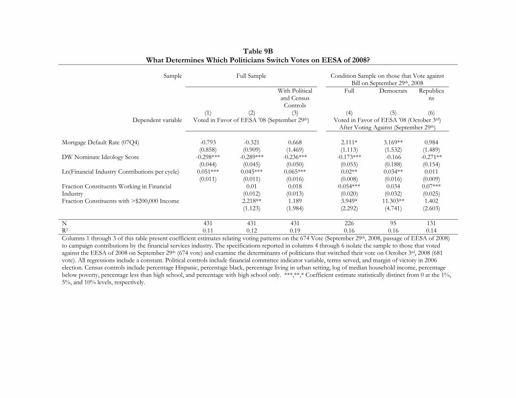
Table 9B What Determines Which Politicians Switch Votes on EESA of 2008?
Sample Full Sample Condition Sample on those that Vote against
Bill on September 29th, 2008 With Political
and Census Controls
Full Democrats Republicans
(1) (2) (3) (4) (5) (6)Dependent variable Voted in Favor of EESA ’08 (September 29th) Voted in Favor of EESA ’08 (October 3rd)
After Voting Against (September 29th) Mortgage Default Rate (07Q4) -0.793 -0.321 0.668 2.111* 3.169** 0.984 (0.858) (0.909) (1.469) (1.113) (1.532) (1.489)DW Nominate Ideology Score -0.298*** -0.289*** -0.236*** -0.173*** -0.166 -0.271** (0.044) (0.045) (0.050) (0.055) (0.188) (0.154)Ln(Financial Industry Contributions per cycle) 0.051*** 0.045*** 0.065*** 0.02** 0.034** 0.011 (0.011) (0.011) (0.016) (0.008) (0.016) (0.009)Fraction Constituents Working in Financial 0.01 0.018 0.054*** 0.034 0.07***Industry (0.012) (0.013) (0.020) (0.032) (0.025)Fraction Constituents with >$200,000 Income 2.218** 1.189 3.949* 11.303** 1.402 (1.123) (1.984) (2.292) (4.741) (2.603) N 431 431 431 226 95 131R2 0.11 0.12 0.19 0.16 0.16 0.14Columns 1 through 3 of this table present coefficient estimates relating voting patterns on the 674 Vote (September 29th, 2008, passage of EESA of 2008) to campaign contributions by the financial services industry. The specifications reported in columns 4 through 6 isolate the sample to those that voted against the EESA of 2008 on September 29th (674 vote) and examine the determinants of politicians that switched their vote on October 3rd, 2008 (681 vote). All regressions include a constant. Political controls include financial committee indicator variable, terms served, and margin of victory in 2006 election. Census controls include percentage Hispanic, percentage black, percentage living in urban setting, log of median household income, percentage below poverty, percentage less than high school, and percentage with high school only. ***,**,* Coefficient estimate statistically distinct from 0 at the 1%, 5%, and 10% levels, respectively.

Table 10
How do Politicians Trade-off Ideology Versus Constituent and Special Interests? With
Political and Census
Controls
With Political and
Census Controls
Sample Republicans only Full sample (1) (2) (3) (4) (5) (6)
Dependent Variable Voted in Favor of AHRFPA ’08 Voted in Favor of EESA ‘08 DW Nominate Ideology Score 1.891* 1.396 1.927 0.218 0.301 0.212 (0.995) (1.136) (0.947) (0.230) (0.301) (0.245)Mortgage Default Rate (07Q4) 21.809*** 19.954*** 17.45 1.294 1.22 0.68 (4.334) (5.918) (10.559) (0.975) (1.271) (6.718)( Ideology Score)*(Mortgage Default Rate) -28.585*** -27.106*** -28.419*** 1.696 2.577 1.652 (7.844) (9.831) (8.008) (2.010) (2.126) (1.976)Ln(Financial Industry Contributions per cycle) 0.094 0.056 0.072 0.071*** 0.085*** 0.067 (0.065) (0.072) (0.095) (0.012) (0.017) (0.050)( Ideology Score)*(Ln(Campaign Contributions)) -0.114 -0.072 -0.118 -0.056*** -0.061*** -0.055*** (0.077) (0.086) (0.073) (0.016) (0.023) (0.018)( Mortgage Default Rate)*(Ln(Campaign Contributions)) 0.38 0.055 (0.762) (0.589) N 192 192 192 432 432 432R2 0.26 0.31 0.26 0.14 0.21 0.14This table examines how politicians trade-off their ideological stance against constituent and special interests. Columns 1 and 2 report specifications examining the determinants of voting behavior on the AHRFPA ’08 501 vote (July 26th, 2008). Columns 3 and 4 report specifications examining the determinants of voting behavior on the EESA ’08 681 vote (October 3rd, 2008). All regressions include a constant. Political controls include financial committee indicator variable, terms served, and margin of victory in 2006 election. Census controls include percentage Hispanic, percentage black, percentage living in urban setting, log of median household income, percentage below poverty, percentage less than high school, and percentage with high school only. ***,**,* Coefficient estimate statistically distinct from 0 at the 1%, 5%, and 10% levels, respectively.

0.5
1P
rope
nsity
to v
ote
in fa
vor
0 .05 .1 .15Mortgage Default Rate
AHRFPA '08 vote against mortgage default rate in Republican districts
Figure 1
05
10
15
20
25
Num
ber
of D
istr
icts
-.04 -.03 -.02 -.01 0 .01Default Rate Difference
Republican and Democratic Default Rate DifferenceFigure 2

.4.5
.6.7
Pro
pens
ity to
vo
te in
favo
r
9 10 11 12 13Log Financial Sector Campaign Contributions
EESA '08 vote against Log Financial Sector Campaign Contributions
Figure 3
LiberalRepublicans
ConservativeRepublicans
0.2
.4.6
.81
Pro
pens
ity to
vo
te in
favo
r
.02 .04 .06 .08 .1Mortgage Default Rate
AHRFPA '08 vote against change in mortgage default rate: By Ideology
Figure 4

LiberalRepresentatives
ConservativeRepresentatives
0.1
.2.3
Pro
pens
ity to
vo
te in
favo
r
9 10 11 12 13Log Campaign Contributions By Financial Industry
EESA '08 vote against Log Campaign Contributions: By Ideology
Figure 5
10
10.
51
11
1.5
12
Log
Fin
anci
al S
ect
or
Cam
pai
gn C
ont
ribut
ions
-1 -.5 0 .5 1DW-Nominate Score
Log Financial Sector Campaign Contributions Against Ideology
Figure 6

05
10
15
20
25
Nu
mb
er o
f D
istr
icts
(Rep
ublic
an O
nly)
0 .05 .1 .15Mortgage Default Rate
(2007Q4)
01
02
03
04
0
Nu
mb
er o
f D
istr
icts
(Rep
ublic
ans
Onl
y)
0 .02 .04 .06 .08 .1Change in Mortgate Default Rate
(2005Q4 to 2007Q4)
05
10
15
20
25
Nu
mb
er o
f D
istr
icts
(Rep
ublic
ans
Onl
y)
0 20 40 60 80 1002006 Election Vote Difference
01
02
03
0N
um
ber
of
Dis
tric
ts
9 10 11 12 13Log Fin. Sector Contributions
01
02
03
04
05
0N
um
ber
of
Dis
tric
ts
-1 -.5 0 .5 1 1.5DW-Nominate Score
Frequency Distributions Of Our Main R.H.S. VariablesFigure A1

Table A1 Robustness of Constituent Interest Result To Right Tale Of Default Distribution
Right Tale Winsorized At 5% Sample Below 07Q4 Default
Rate
Sample Above 07Q4 Default
Rate (1) (2) (3) (4) Dependent Variable: Voted in favor of AHRFPA '08 (July 26th, 2008)Mortgage Default Rate (07Q4) 7.2*** 11.36*** 8.3*** (1.69) (4.40) (1.98)DW Nominate Ideology Score -0.87*** -0.83*** -0.77*** -0.89*** (0.16) (0.16) (0.21) (0.26)Ln(Financial Industry Contributions per 0.02 0.01 -0.02 0.02cycle) (0.01) (0.01) (0.04) (0.01)Mortgage Default Rate (05Q4) 2.42 (2.34) Mortgage Default Rate (05Q4-07Q4) 8.61*** (1.69) N 192 192 97 95R2 0.21 0.25 0.18 0.27All regressions include a constant. Political controls include financial committee indicator variable, terms served, and margin of victory in 2006 election. Census controls include percentage Hispanic, percentage black, percentage living in urban setting, log of median household income, percentage below poverty, percentage less than high school, and percentage with high school only. ***,**,* Coefficient estimate statistically distinct from 0 at the 1%, 5%, and 10% levels, respectively.
0.2
.4.6
.8P
rop
en
sity
to v
ote
in f
avo
r
0 .01 .02 .03 .04Accounts Divided by Total Population
0.2
.4.6
.8P
rop
en
sity
to v
ote
in f
avo
r.01 .02 .03 .04 .05
Accounts Divided By Pop. with Credit Report
AHRFPA '08 vote against fraction of mortgage accounts in defaultFigure A2

Table A2 Determinants Of Campaign Contribution
Political and Census
Controls
Political and Census
Controls (1) (2) (3) Dependent Variable:
Log Financial Industry Campaign Contribution per Cycle DW Nominate Ideology Score 0.5*** 0.31** 0.29* (0.14) (0.16) (0.17) (DW Nominate Ideology Score)2 -1.94*** -1.96*** -1.89*** (0.63) (0.60) (0.59) Fraction Constituents Working in 0.05 Financial Industry (0.04) Fraction Constituents with >$200,000 8.11* Income (4.49) Constant 11.66*** 6.11 13.68 (0.14) (9.72) (12.30) N 433 433 433 R2 0.06 0.21 0.22 All regressions include a constant. Political controls include financial committee indicator variable, terms served, and margin of victory in 2006 election. Census controls include percentage Hispanic, percentage black, percentage living in urban setting, log of median household income, percentage below poverty, percentage less than high school, and percentage with high school only. ***,**,* Coefficient estimate statistically distinct from 0 at the 1%, 5%, and 10% levels, respectively.