The National MagLab Carlos R. Villa K-12 Education Outreach Coordinator.

The Physics of Noiseand musings on experimental errors ...
Matt Kowitt, Stanford Research Systems

What is noise?Short answer: it’s everything you don’t want
Similar to a gardener’s definition of “what is a weed?”

Why should you care?• You want your measurements to be right.
• You want to be able to communicate your results successfully.
As an experimental physicist, you should expect to spend much of your career dealing with low signal-to-noise ratios.
Ultimately, you are trying to make some measurement, along with your best estimate of the uncertainty in that measurement.

Importance of noise (and errors generally)When designing an experiment, you should understand—quantitatively—the
sources of noise and systematic errorsKeep checking: if more noise than anticipated, you’ve got more work to do
Track down and fix the additional noise sources
Too little noise: likely a problem tooThe universe never gives you such gifts — more likely, something is broken!
Remain skeptical of your results
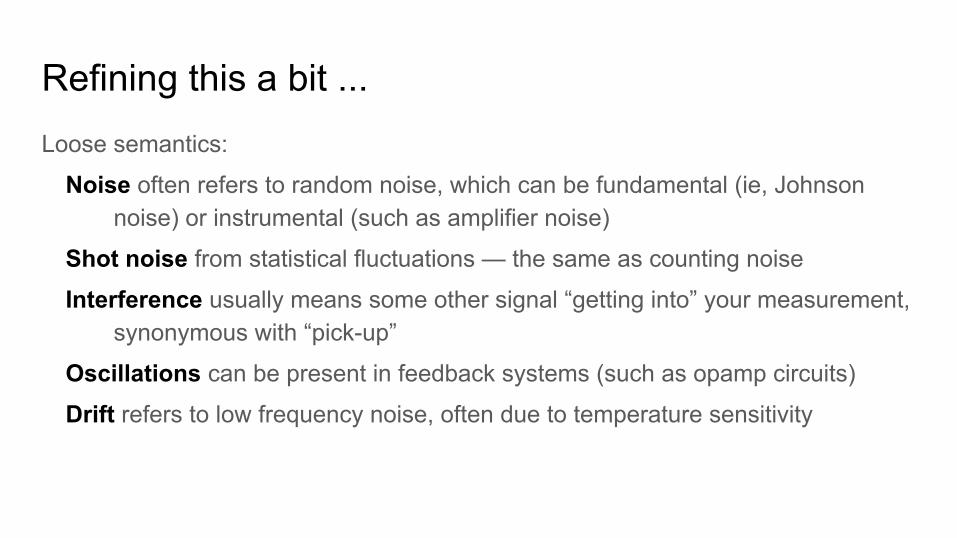
Refining this a bit ...Loose semantics:
Noise often refers to random noise, which can be fundamental (ie, Johnson noise) or instrumental (such as amplifier noise)
Shot noise from statistical fluctuations — the same as counting noise
Interference usually means some other signal “getting into” your measurement, synonymous with “pick-up”
Oscillations can be present in feedback systems (such as opamp circuits)
Drift refers to low frequency noise, often due to temperature sensitivity

Noise is (usually) made of fluctuations about zeroAverage about mean is (by
definition): 〈V-〈V〉〉=0Convenient to define noise as
zero-averaged, 〈V〉=0Average power (V2) ≠0
But it’s hard to think in volt2, so typically use RMS (square Root of the Mean of the Squared signal)
VRMS= √〈V2〉

How to calculate noise from PSDPower Spectral Density ⇒ power per unit bandwidthNoise adds incoherently
⇒ add power, not amplitudeTHS4131 opampTo estimate RMS noise within some
frequency band, integrate the area as power, or V2/Hz.
⇒ square to voltage noise, then integrate, and then square root for Vrms

Example: calculating RMS estimate
For THS4131, en≅ 1.45 nV/√Hz; fknee≅ 325 Hz
(Vn)2 ≅ (en)
2 (1+ (fknee/f) )
To estimate the RMS noise from 1 Hz to 10 kHz:
<VRMS> =√ { ∫1 Hz [(en)2(1+ (fknee/f) )] df }
= en√ {(10kHz-1Hz) + fknee(ln(10kHz / 1 Hz))}= en√ {9999 Hz + 2993 Hz}= 165 nVrms
Aside: did you notice how 1/f noise has constant power per decade?
THS4131 opamp

A bit more about Power Spectral Density● Useful for describing “stationary” noise (properties not changing over time)● For “ergodic” stationary noise (ensemble averages = time averages), we have
○ Autocorrelation function of noise is the Fourier transform of the PSD○ Autocorrelation function S(τ) = 〈 x(t) x(t-τ) 〉○ This is the basis for a trick for measuring a sample’s PSD below the noise power of amplifier
measure the signal with two separate amplifiers, then take FFT of cross-correlation

Fundamental noise source #1: Johnson NoiseThermal motion of electrons
ALL resistors exhibit Johnson noise
Flat* power spectral density, en2=4kTR
Rules of thumb (for 300 K):1 kΩ ⇒ 4.07 nV/√Hz ≅ 4 nV/√Hz
50 Ω ⇒ 0.91 nV/√Hz ≅ 1 nV/√Hz
k = Boltzmann constant,1.38⨉10-23 J/K
*: spectrum is flat up to THz frequencies at room temperature

Johnson noise, continuedElectrically, a physical resistor at temperature T (A) is equivalent to
(B) a noiseless resistance in series with a voltage noise source, or
(C) a noiseless resistance in parallel with a current noise source
Leads to (perhaps) surprising noise property of transimpedance amplifier (I-to-V)
Gain = R (V/A)Noise (RTI) = √(4kT/R)Larger R ⇒ smaller (current) noise
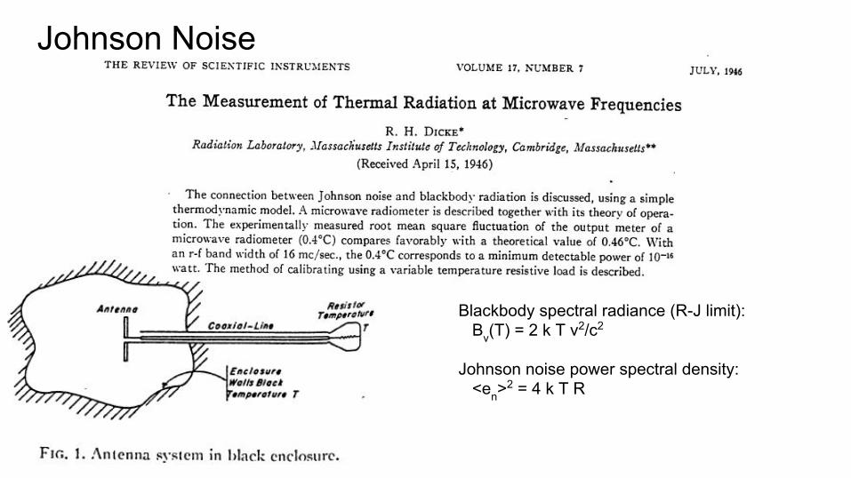
Johnson Noise
Blackbody spectral radiance (R-J limit): Bν(T) = 2 k T ν2/c2
Johnson noise power spectral density: <en>
2 = 4 k T R
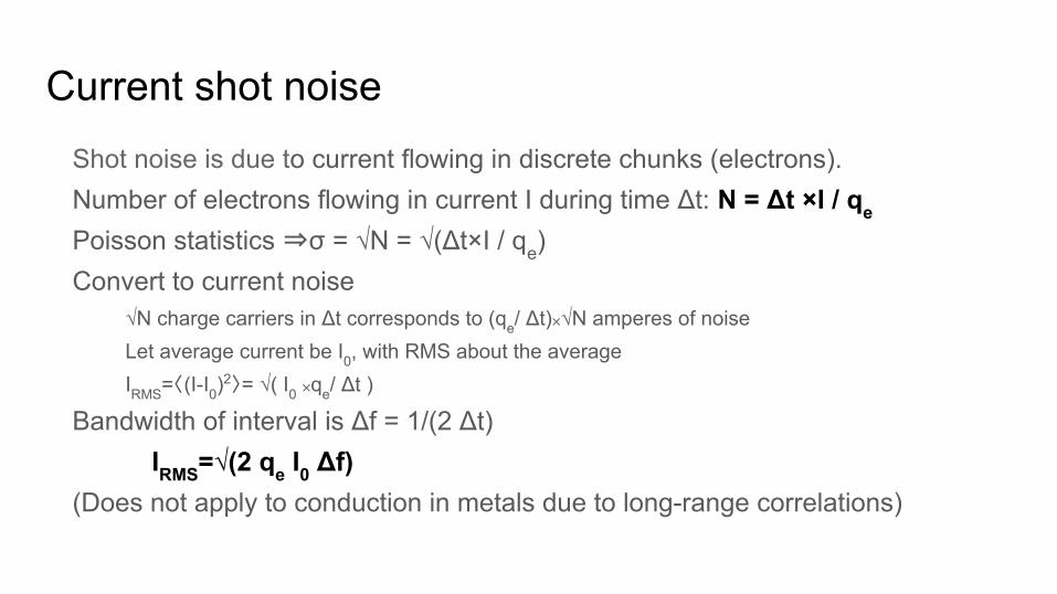
Current shot noiseShot noise is due to current flowing in discrete chunks (electrons).Number of electrons flowing in current I during time Δt: N = Δt ×I / qe
Poisson statistics ⇒σ = √N = √(Δt×I / qe)Convert to current noise
√N charge carriers in Δt corresponds to (qe/ Δt)⨉√N amperes of noiseLet average current be I0, with RMS about the averageIRMS=〈(I-I0)
2〉= √( I0 ⨉qe/ Δt )
Bandwidth of interval is Δf = 1/(2 Δt)IRMS=√(2 qe I0 Δf)
(Does not apply to conduction in metals due to long-range correlations)

1/f noisePronounced “one over eff”;
sometimes called flicker noise
Power spectral density scales as ∝f -1 (or close to -1)
Many (many!) systems exhibit 1/f noise
One of the reasons lock-in amplifiers are handy

More examples
From “Low Level Measurements Handbook – 7th Edition”, Keithley
From “Resistor Current Noise Measurements”, LIGO-T0900200-v1

Amplifier noise: SR560 as exampleNoise power spectrum is a good starting point:

SR560 continued: noise figure
1/f
Input capacitance
Input bias current

External noise sources• Minimize by good design• Averaging may or may not help
• Depends on correlation with signal• Saturation or other non-linearities

Capacitive pick-up
Noise currentI = Cstray dV/dt = 2 f Cstray Vnoise
example:f = 60 Hz, Vnoise=120 Vrmsarea is 1 cm2, gap is 10 cm
⇒ Cstray≅ 9 fFthen the picked-up current noise would be:
I = 2 f Cstray Vnoise= 40 pA
How to mitigate:1. Remove or turn off noise
source2. Add distance (reduce Cstray)3. Design to measure at voltage
at low impedance4. Grounded shielding

Inductive coupling
Nearby equipment with AC current can couple to the experiment via magnetic flux.
Effectively creates a transformer, where the experiment-detector loop becomes the secondary winding
How to mitigate:1. Remove or turn off noise
source2. Reduce area of pick-up loop
by using twisted pairs, coaxial cables, etc.
3. Use magnetic shielding to prevent flux lines from crossing area of experiment
4. Measuring currents, not voltages, from high impedance detectors

Resistive coupling or ground loops
Currents flowing through ground connections give rise to noise voltages
Ground loops are ubiquitous! Think of the many BNC interconnections tying chasses together...
RGroundHow to mitigate:
1. Single-point grounding 2. Heavy ground bus to reduce
RGround resistive burden3. Remove sources of large
ground currents from ground bus for small signals
4. Using differential excitations and signal sensing

Lead resistanceSimilar to the ground loop problem: resistive drops along lead wires causes measurement error.
Solution: 4-wire circuit: separate the excitation current leads from the voltage sensing leads.
From “Low Level Measurements Handbook – 7th Edition”, Keithley

OscillationsTypically from feedback circuits (op amps) with insufficient phase margin
Tempted to just “filter it out”? Don’t. You need to fix this!
Oscillating amplifier more likely to become nonlinear. The extra ac ripple exacerbates capacitive pickup. Common source: driving cables (capacitive load) directly from op amp output. Try putting a small (50 Ω) resistor in series.
oscillation

AC InterferenceIn addition to being a noise source, RF pickup can cause DC errors due to rectification.
Also, beware of AC power being coupled into sensitive samples where it can cause unexpected self-heating or other problems.
Temperature shifts due to voltage noise across silicon diode temperature sensor
From Temperature Measurement & Control Catalog, Lakeshore Cryotronics

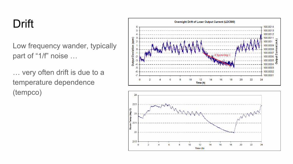
Drift
Low frequency wander, typically part of “1/f” noise …
Drift
Low frequency wander, typically part of “1/f” noise …
… very often drift is due to a temperature dependence (tempco)
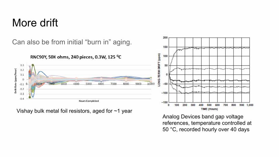
More driftCan also be from initial “burn in” aging.
Analog Devices band gap voltage references, temperature controlled at 50 °C, recorded hourly over 40 days
Vishay bulk metal foil resistors, aged for ~1 year

Other sources of noise
From “Low Level Measurements Handbook – 7th Edition”, Keithley
Triboelectric: charge transfer due to friction
Microphonics: e.g. wires vibrating create Δcapacitance ⇒ voltage & currents
From “Principles of dilution refrigeration”, Oxford Instruments
Copper braids decouple pulse tubes from experimental plates

Thermoelectric: Seebeck effect
From Jim Williams et al, Ap Note 86, Linear Technology (2001)
● Junctions of dissimilar metals generate thermal EMF, typically fraction of µV/°C
● Universally plagues microvolt level DC circuits
From “Low Level Measurements Handbook – 7th Edition”, Keithley

Checking for spurious results...Consider this double lock in experiment: recall ΔRXX≅10-4RXX
⇒ worry about false signal from microwave source
• could the modulating source cause pickup in L2 (or L1)?
• ways to test against this:• keep 5.7 Hz modulation, but block
microwave path to sample• try steady microwave source, add
modulation with, e.g., a chopper

Understanding noise sources: the 1972 LIGO design noteR. Weiss documented all the significant noise sources for LIGO 44 years before the first detection.Useful example of how to systematically understand the sources of noise that will contribute to a measurement
RLE QPR No 105 (1972)http://hdl.handle.net/1721.1/56271

Analysis of 9 contributing noise sources:1. Amplitude Noise in the Laser Output Power2. Laser Phase Noise or Frequency Instability3. Mechanical Thermal Noise in the Antenna4. Radiation-Pressure Noise from the Laser Light5. Seismic Noise6. Thermal-Gradient Noise7. Cosmic-Ray Noise8. Gravitational-Gradient Noise9. Electric Field and Magnetic Field Noise

Just look at Amplitude Noise termAbility to measure an interferometer fringe is limited by shot noise fluctuations in the arrival rate of photons. Weiss translated this into a displacement power spectral density [units m2/Hz]
where h is Planck’s constant, c the speed of light, λ the laser wavelength, ε the quantum efficiency of the photodetector, P the laser power, b the number of passes in each interferometer arm, and R the mirror reflectivity.
The noise power has a minimum for b = 2(1-R).

Amplitude noise from LIGO laser output power Example values from 1972 paper
P = 0.5 Wλ = 500 nmR = 99.5%ε = 50%
Δx2(f) / Δf ≥ 2.3×10-37 m2/Hzstrain ≥ 1.2×10⁻²² /√Hz
Updating for 2015 Adv LIGO
P = 20 Wλ = 1064 nmR = 99.9%ε = 90%
Δx2(f) / Δf ≥ 4.1×10-40 m2/Hzstrain ≥ 4.1×10⁻²⁴ /√Hz
convert to strain noise currently used in LIGO papers by using interferometer arm length L=4km, strain noise = (1/L) √[Δx2(f) / Δf ]

photon shot noise limited ≳ 150 Hz, ~7×10-24 /√Hz

Example of signal-free dataset for end-to-end checkCOBE: Cosmic Background Explorer
Launched Nov 1989
DMR experiment to measure anisotropy in the CMB

The DMR experiment6 differential microwave radiometers: 2 identical channels (A & B), at frequencies 31.5, 53, and 90 GHz.
Each measures power difference in two 7° beams separated by 60°, each 30° from the spacecraft spin axis.
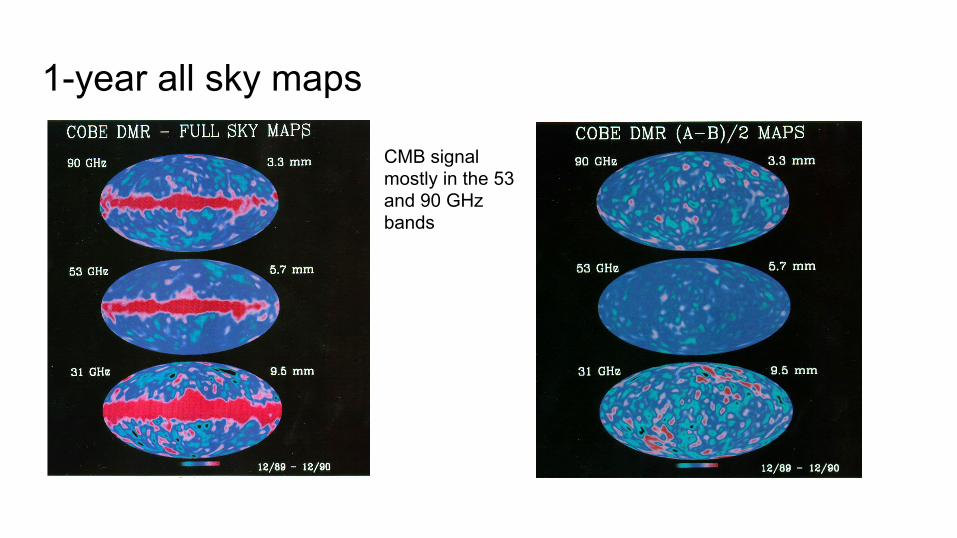
1-year all sky maps
CMB signal mostly in the 53 and 90 GHz bands

Convincing a skeptical worldCOBE DMR required an elaborate data analysis to generate sky maps free from artifacts:
Measuring part-in-105 differences in the 2.7K microwave background, while orbiting a 300K planet with the moon and Jupiter overhead, a 5800K sun nearby, and sensitivity to external magnetic field
The “A–B” results help convince that the derived signal is not spurious