The Phillips Curve and The Great Recession.
34
Bachelor Thesis, 15 credits Economics C100:2 Spring 2019 The Phillips Curve and The Great Recession. A cross-section comparison among eight European countries between 2000-2017. Hanne Måseide
Transcript of The Phillips Curve and The Great Recession.

Bachelor Thesis, 15 credits
Economics C100:2
Spring 2019
The Phillips Curve and The Great
Recession. A cross-section comparison among eight European countries
between 2000-2017.
Hanne Måseide

2
Abstract
The idea behind this bachelor thesis comes from findings of a study made by L. M. Ball &
Mazumder (2011). After 2008, the unemployment rate in the U.S started to rise which according
to predictions from the Phillips inflation should turn into deflation. Although, the U.S faced a
different outcome. The results from their study indicated that the Phillips curve has been
performing poorly after the Great Recession and they stated that the credibility of the Phillips
curve can be questioned.
This study aims to analyze the relationship between the unemployment rate and inflation,
known as the Phillips curve, in eight European countries. It further aims to investigate if the
Great Recession had any effect on the relationship. This is made by using annual data over the
time period of 2000-2017.
The results show that there exist country-specific differences in four out of the eight countries
included in the study. It also shows that the relationship between unemployment and inflation
is weakest in Italy and strongest in France. Furthermore, the study could show that the
relationship had become stronger after the Great Recession in France, Finland, and Italy.

3
Table of content 1. INTRODUCTION ................................................................................................................................. 4
2. THEORETICAL FRAMEWORK ......................................................................................................... 6
THE ORIGINAL PHILLIPS CURVE ........................................................................................................................ 6
3. LITERATURE REVIEW ................................................................................................................... 14
DATA .................................................................................................................................................................. 18 MODELS AND METHOD ..................................................................................................................................... 20
5. RESULT ............................................................................................................................................. 23
6. DISCUSSION ...................................................................................................................................... 29
REFERENCE LIST ................................................................................................................................ 32
APPENDIX ............................................................................................................................................. 34

4
1. Introduction
After the Great Recession, which begun in the U.S during the year of 2008, many countries in
the world faced a decline in economic activity. This decline had several economic
consequences, such as increased unemployment rate and a decrease in inflation. Around the
world, Central Banks attempted to fight these economic consequences by stimulating the
economy by lowering the interest rate. Since then, interest rates have continuously been kept
low and in 2014, the European Central Bank pushed the boundaries even further by cutting the
interest rate below zero. A negative interest rate are an unconventional tool in monetary policy
and implies that private banks have to pay a deposit to keep their money in the Central Bank.
The theory behind it is that it will drive the initiative for private banks to increase their lending’s
to consumers and companies and thereby stimulate the economy through consumption and
investments. In a historical perspective, negative interest rates is a untested method and
therefore makes the outcome uncertain. Even though the interest rates have been kept low and
unemployment have continued to fall, inflation has shown a very slow increase. In fact, it still
remains below the set targets in many advanced economies (Hong, Koczan, Lian, & Nabar,
2018).
The Phillips curve is an economic model suggesting a negative relationship between the
unemployment rate and inflation. The model, therefore, implies that a fall in unemployment
should lead to an increase in inflation. As the model has been considered to generate reliable
predictions of inflation, it has been well used by politicians and economists to predict future
inflation for a long time. However, doubts among economists about whether the Phillips curve
is an appropriate model to forecast inflation have grown in recent years. And this is not the first
time doubts occur. The doubt is based upon the issues which presented itself during, and after,
the Great Recession. During the Recession, the U.S faced a rise in the unemployment rate and
according to predictions from the Phillips curve, the rise in the unemployment rate should have
yielded a greater decrease in inflation. Much greater than the decrease the U.S. experienced. It
seems like the relationship between inflation and unemployment, once regarded reliable, has
weakened (L. Ball & Mazumder, 2014). Researchers have been trying to understand why
inflation has been behaving in this way, and several possible explanations have been brought
to attention – some of which will be discussed in this paper.

5
The purpose of this paper is to study the relationship between the unemployment rate and
inflation, known as the Phillips curve, in eight advanced European economies. This paper
further aims to analyze whether the Great Recession had any impact on the reliability of the
Phillips curve. If the relationship has changed, a relevant and essential question to be answered
would be whether the Phillips curve should continue to play an important role in the monetary
policy of these countries.
This study is limited to include eight countries namely Denmark, Finland, France, Germany,
Italy, Norway, Sweden, and the United Kingdom. The main argument for the particular
selection of countries is the desire to study relatively homogeneous countries in the analysis.
This study will be limited to include annual data over the time period of 2000-2017. By
restricting the time period, the study will not become too comprehensive but still allow for an
analysis of the effect on the Phillips curve caused by the financial crisis.
The theoretical framework will be presented in section two, followed by the literature review
in the third section. In section four the method is described including summarizing data and
econometric approach used. The fifth section includes the empirical results and finally, the
discussion is presented in the sixth section.

6
2. Theoretical framework
The Original Phillips curve
Phillips (1958) presented a study on the relationship between wages and inflation in the U.K
economy, a study which later on turned out to be of great importance for monetary policy.
Phillips found evidence that there existed a strong negative relationship between wage levels
and inflation. A few years later, Samuelson and Solow (1960) found that wages and prices were
correlated. If wages increased, prices were going to increase as well. Thereby, a negative
relationship between the unemployment rate and inflation was discovered, which implies that
high unemployment indicates low inflation and vice versa. This relationship was accepted and
adopted by many economists for years to come and was famously known as the Phillips curve.
The original Phillips curve implied a trade-off between inflation and unemployment, which
appeared to give politicians the opportunity to select a desired level of inflation by accepting a
certain level of unemployment. During 1970, many countries faced, in contrast to what the
Phillips curve was predicting, high inflation along with a high level of unemployment. The high
unemployment and inflation gave rise to suspicions regarding the reliability of the relationship
and subsequently got questioned by economists. This phenomenon was assumed to be a
consequence of a change in the behavior of inflation. Inflation had become more persistent
which changed the way wage setters formed their inflation expectations. If inflation was high
today, it was likely that it would be high tomorrow as well. Wage setters and price setters started
to take the persistence of inflation into account, which led them to expect inflation next year to
be the same as it was the year before. As a result, inflation expectations started to have an
impact on inflation and it, therefore, became important to take that into account when
attempting to forecast the inflation. The original Phillips curve was now modified and showed
a negative relationship between the unemployment rate and changes in inflation. Low
unemployment rate indicated for an increase in inflation rate and vice versa. The new modified
Phillips curve is often called the accelerationist Phillips curve (Blanchard, Amighini, &
Giavazzi, 2017).
7
The original Phillips curve has also received criticism from both Friedman and Edmund Phelps
(Phelps, 1967). They argued that since the unemployment rate is converting to its equilibrium
in the long run, the relationship only exists on a short-term basis. Further, they argued that there
is only one specific level of unemployment that is consistent with a stable level of inflation.
The unemployment rate that generates stable inflation is called Non-accelerating Inflation Rate
of Unemployment (NAIRU). The economy is going to be at this level when wages are constant,
and the price level is at its expected level.
Phelps (1967) further argued that for inflation to change, unemployment needs to deviate from
its equilibrium. The criticism was taken into consideration in the modification of the Phillips
curve along with that was the unemployment gap included. The modified Phillips curve,
presented below, is the relationship which will be analyzed in this thesis. The relationship will
further on be referred to as the Phillips curve.
𝜋𝑡 = 𝜋𝑡−1𝑒 + 𝛼(𝑢𝑡 − 𝑢𝑛)
Where 𝜋𝑡 is the actual inflation in period t, 𝜋𝑡−1𝑒 is the expected inflation in period t-1, 𝑢𝑡 is
the actual unemployment at period t, 𝑢𝑛 represents NAIRU and (𝑢𝑡 − 𝑢𝑛) is the unemployment
gap which shows how much the actual unemployment deviates from NAIRU. is the Phillips
curve coefficient showing the slope of the Phillips curve which tells us how strong the
relationship is i.e how changes in the unemployment gap will affect inflation. When the
unemployment rate is higher than its natural rate, inflation is expected to fall, and when it is
lower, inflation can be expected to rise (L. M. Ball & Mankiw, 2002).
The Unemployment gap model
There are several different versions of the Phillips curve, but common for everyone is that they
show a relation between the resource utilization in the economy and changes in the level of
inflation. Resource utilization can be represented by either the output gap or the unemployment
gap, where the latter will be used in this study. The unemployment gap shows how far away
the labor market is from its equilibrium, NAIRU, which is considered to indicate maximum
resource utilization. NAIRU represents the structural unemployment within an economy and
arise from rigidities on the labor market and when it exists no labor demand. The structural
8
unemployment is, for example, affected by mismatches between vacancies and hires as well as
labor demand and changes in social welfare programs (Blanchard et al., 2017).
The theory behind the Phillips curve, how inflation and unemployment are linked together,
comes from the labor market and how the bargaining power of the unions affect wages. The
relationship works in this way: When the actual unemployment rate is low, fewer people are
searching for jobs which means that there is higher competition for firms among the workers
when they need to hire. When the competition for workers is high, the unions can bargain for
higher real wages. Higher real wages leads to an increase in real wage-costs for the firms and
in order to compensate for those higher costs, firms raise their prices. Since inflation is a
measure of price changes, higher prices will indicate higher inflation.
Inflation expectations
Inflation expectations play an important role in the determination of inflation. As the expected
inflation is being taken into consideration when firms and households make decisions about
wage contract negotiation and price-setting, these decisions will, in turn, affect the actual
inflation (Bullard, 2016). There are two different approaches to how individuals expect next
year's inflation, these are rational and adaptive theories. Adaptive inflation expectations can be
seen as a backward-looking approach assuming people to base future predictions about inflation
on historical data. For instance, if inflation is high today, people would expect inflation to be
high in the future as well. This approach can, however, be seen as rather simplified. In the real
world, historical data is just one of the many things that influence inflation. Rational inflation
expectation approach is a form of forward-looking expectations. In this approach, people are
assumed to use all information accessible, except historical data, to predict next year’s inflation.
For example, people expect inflation to increase if the government increases their spending’s
and they act upon it right away by, for example, bargain for higher real wages. However,
rational expectations rely on consumer having a strong knowledge and insight in the economy
which not always is the case. Adaptive inflation expectations will be used in this study as that
gave the most significant results.

9
The slope of the Phillips curve
For the sake of convenience, we assume that the economy is closed and therefore, the slope of
the Phillips curve will not be affected by any global factors. The slope of the Phillips curve is
represented from is determined by the slope of the wage setting-curve (WS), that together
with the price setting-curve (PS) shows the equilibrium on the labor market (see figure 1 below).
The slope of the WS-curve is determined by the wage-setting relation:
𝑊
𝑃= 𝐹(𝑢, 𝑧)
The equation above shows that real-wages is a function of unemployment, u, and other
variables, z, that may affect the wage setting, for example, union density and unemployment
protection. The function implies a negative relationship between the unemployment rate and
the real wage: an increase in unemployment will have a decreasing effect on real wages. The
wage setting curve, therefore, shows how much real wages need to increase in order to make
the unemployment rate diverge from the equilibrium and attract one extra unit of employment.
Which later will have an increasing effect on the inflation rate (Blanchard et al., 2017).
The PS-curve is determined by the price-setting relation:
𝑊
𝑃=
1
1 + 𝑚
The price-setting shows that real-wages paid by firms are equal to firms price-setting behavior,
1
1+𝑚, where m represents the mark-up of prices over cost (Blanchard et al., 2017). The price-
setting behavior by firms do not depend on the unemployment rate and is therefore drawn as a
horizontal line in Figure 1 below.
Illustrations over the labor market and the Phillips curve can be found in Figure 1 below. The
vertical Phillips curve (VPC) represents NAIRU which in turn shows the equilibrium on the
labor market in the long run.
(-,+)
10
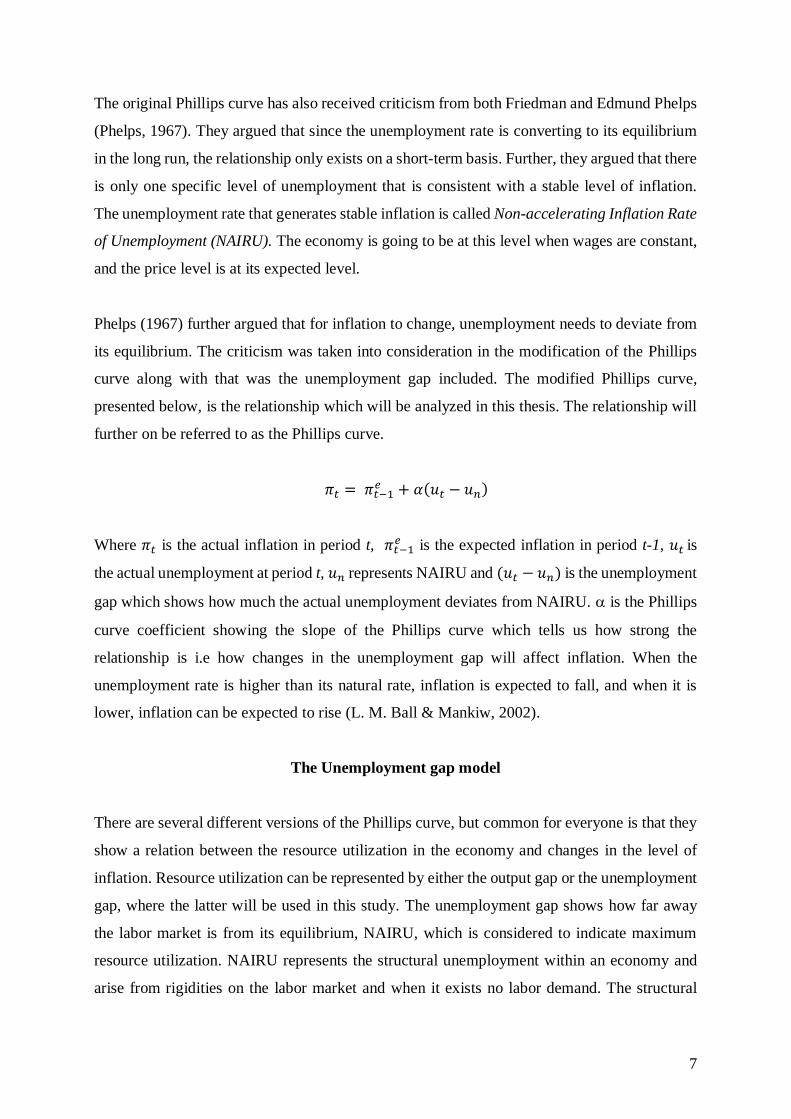
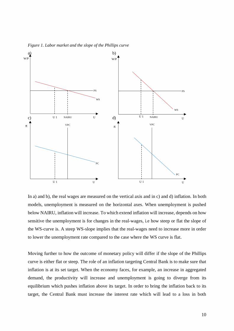
Figure 1. Labor market and the slope of the Phillips curve
a) b)
c) d)
In a) and b), the real wages are measured on the vertical axis and in c) and d) inflation. In both
models, unemployment is measured on the horizontal axes. When unemployment is pushed
below NAIRU, inflation will increase. To which extend inflation will increase, depends on how
sensitive the unemployment is for changes in the real-wages, i.e how steep or flat the slope of
the WS-curve is. A steep WS-slope implies that the real-wages need to increase more in order
to lower the unemployment rate compared to the case where the WS curve is flat.
Moving further to how the outcome of monetary policy will differ if the slope of the Phillips
curve is either flat or steep. The role of an inflation targeting Central Bank is to make sure that
inflation is at its set target. When the economy faces, for example, an increase in aggregated
demand, the productivity will increase and unemployment is going to diverge from its
equilibrium which pushes inflation above its target. In order to bring the inflation back to its
target, the Central Bank must increase the interest rate which will lead to a loss in both
U
W/P
PS
WS
NAIRU
U
PC
VPC
NAIRU U
U
W/P
U 1
U 1
U 1
U 1
PS
WS
PC
VPC

11
productivity and unemployment. How big the loss will be is determined by the slope of the
MR-curve and the Phillips curve. The MR-curve shows the Central Banks preferences. A
Central bank can either be inflation averse or unemployment averse. An inflation averse Central
Bank place more weight on deviations in inflation from its target than on deviations in
unemployment. So a more inflation averse Central Bank is more willing to accept a greater loss
in employment to reduce inflation that an unemployment averse Central Bank. A steep MR-
curve indicates for an inflation-averse Central Bank and a flat slope shows the opposite. For
simplicity, assume that the slope of the MR-curve is equal to 1, which implies that the Central
Bank is indifferent between having unemployment below or inflation above its target. The only
thing that now decides how big reduction in production and unemployment that needs to be
accepted to reach the inflation target is the slope of the Phillips curve. To show this, two
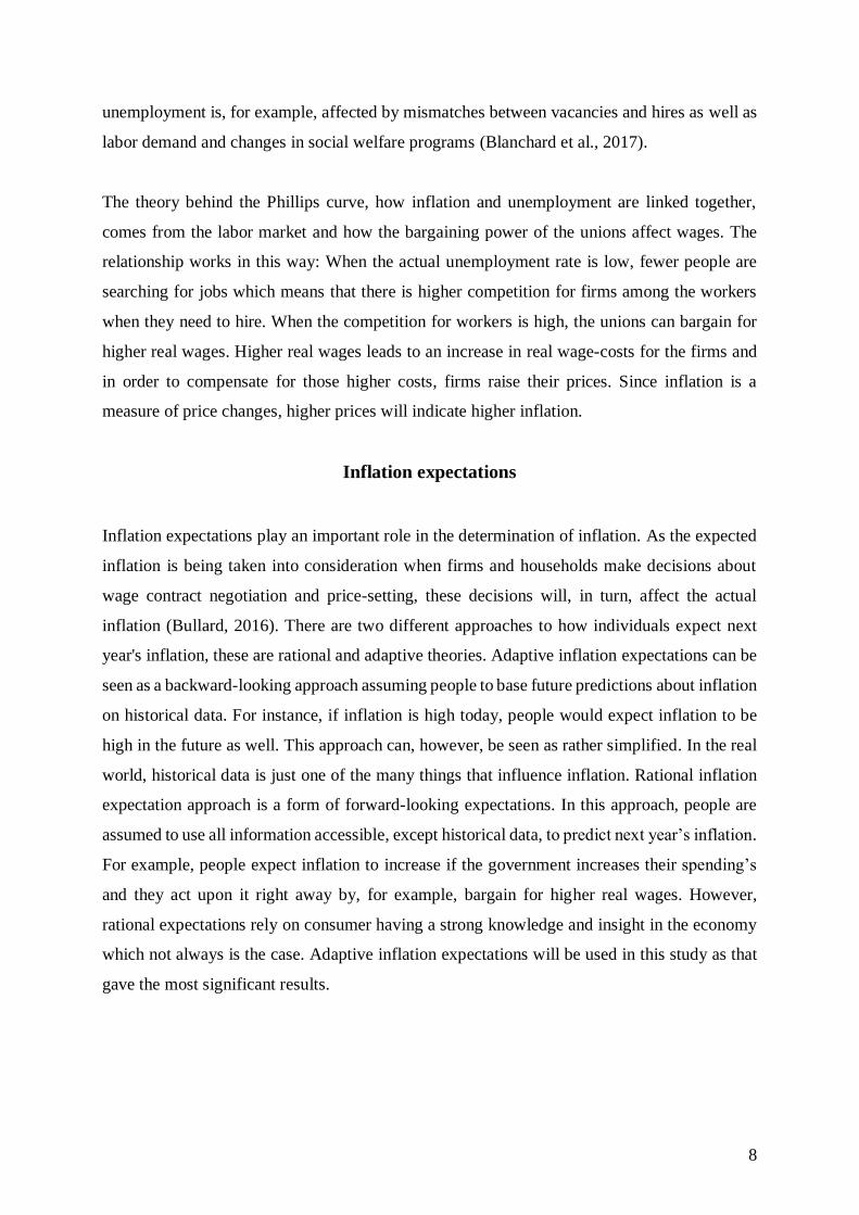
possible cases have been illustrated in Figure 2 below. On the vertical axes, production (y) is
measured and on the horizontal axes inflation ().
a)
The economy moved from point A to point B due to the increase in aggregated demand.
Production has moved from y* to y1 and inflation has increased from 2 percent to 6 percent. In
order to bring back the inflation to its target, point A, the Central Banks needs to increase the
interest rate. The extent of the increase is determined by the slope of the Phillips curve. In
Figure 2 a), we have a flat curve compare to in b) where the slope is steep. A steep Phillips
curve indicates that a small reduction in unemployment is required for a large reduction in
inflation, compared to a flat Phillips curve which indicates that a big reduction in
unemployment is needed in for a small reduction in inflation.
What are the implications for monetary policy when the Phillips curve is flatter? Since a flat
Phillips Cure indicates that the sensitivity of wages to demand shock is being reduced and
Inflation Target
VPC
MR
2%
4%
6% PC 2%
PC 4% PC 4%
PC 2% MR
VPC
Inflation Target
4%
6%
2%
y
B
A A
B
C
C
y 2 y 1 y*
y* y 2 y 1
b)

12
therefore put less pressure on inflation. Iakova (2014) states that on one hand, the Central Bank
needs to have a more contractionary monetary policy and move the interest rate more in order
to decrease the aggregated demand and bring back the inflation to its target. And on the other
hand, a flatter Phillips curve can make their job easier since they do not have to worry so much
when the economy faces temporary imbalances between supply and demand.
Potential problems with the Phillips curve
There are some potential problems with the relationship between inflation and unemployment
which is essential to consider while designing macroeconomic policies. Since resource
utilization cannot be observed directly, the use of the different between NAIRU and the actual
unemployment rate makes the model rather simplified (Swedish Central Bank, 2016). NAIRU
also varies over time and it is therefore difficult to estimate the correct level (Bergstr & Boije,
2005). L. M. Ball & Mankiw (2002) says that why NAIRU changes over time is a difficult
question to answer. A potential explanation that they highlight is a phenomenon called
hysteresis which can occur on the labor market. L. M. Ball and Mankiw (2002) explain
hysteresis as follow:
“In physics, hysteresis refers to the failure of an object to return to its original value after being
changed by an external force, even after the force is removed.” (p. 119)
Hysteresis arises in the labor market if the past unemployment rate affects its natural rate. Here
is an example of how it works: People who lose their job due to a decrease in demand might
after a while become demotivated and lose human capital. That will make them less employable
which in turn will reduce their chances of future employment despite a potential recovery in
employment levels. Firms may also be more unwilling to hire people that have been without
work for a certain period. So, workers who first become cyclical unemployed turns into being
structural unemployed and therefore, the economy faced and permanent change in NAIRU.
Inflation can be affected by many different things than those captured by resource utilization.
For example, greater openness to foreign trade, also referred to as globalization, that many
countries face today. When companies face an increase in competition from abroad, economists
argue that, even if unemployment is low and the real-wages have increased, companies cannot
raise their prices as much as before. So, even if the domestic unemployment has change or the

13
real-wages have increased inflation will not be affected (L. M. Ball & Mankiw, 2002). Another
factor that can cause problems is if the inflation expectations have been estimated poorly and if
the expectations differ from the actual expectations.

14
3. Literature review
As described in the introduction, the Phillips curve shows a negative short-run relationship between
unemployment and inflation. This relationship has been developed from being credible to has collapsed
and in recent time, economists have found that the relationship now seems to have weakened again. There
are several studies made on the U.S economy, for example, L. M. Ball & Mazumder (2011) and (Binder,
2016). The results from the studies show that the Phillips curve has been performing poorly after the Great
Recession. As a consequence of the findings, arguments have been presented that the reliability of what
this relationship implies can be questioned.
Since 2008, U.S economy has faced a positive unemployment gap. According to the theory behind the
Phillips curve, a positive unemployment gap should yield a fall in inflation. But the result from a study
made by L. M. Ball & Mazumder (2011) presented the opposite outcome. Historical data from the Phillips
curve were used in order to forecast the inflation from 2008 to 2010. What they found was puzzling. The
predictions indicated that inflation should have been falling into deflation, although, the actual inflation
stayed positive. Since the actual inflation has remained positive and stable, Gordon (2013) states that the
Phillips curve and its credibility can be questioned and in an article published in The Economist (2017)
the author states that “The Phillips curve may be broken for good”. The reason why many economists
have questioned the credibility is illustrated by Ball & Mazumder, (2011) in figure 2 below.
Figure 2.
The figure shows that predictions from the Phillips curve implicated the inflation to fall into
deflation. But as the line representing the actual inflation shows, the outcome became the
opposite.

15
There are several opinions among economists about why this puzzle has emerged, for example, Simon et
al (2013) and Coibion & Gorodnichenko (2015). Simon et al. (2013) highlight the fact that the relationship
also seems to have become weaker within several advanced economies within the OECD. In contrast to
the outcome from Great Recession, previously recessions have been followed by a larger decline in
inflation. One explanation behind why inflation stayed positive instead of turning into deflation is,
according to Simon et al. (2013), that a considerable share of the increase in unemployment was structural.
As a consequent of that, high level of unemployment did not influence inflation as much as it has done in
the past.
Another theory for why inflation did not fall as much as expected, puts focus on the behavioral of inflation.
Simon et al., (2013) found that over the past two decades, Central Banks have been more successful
in delivering stable inflation over time. Therefore, inflation expectations have become more
anchored to the inflation target set by the Central Bank. That has resulted in people thinking
about future inflation in a new way and this, in turn, influences inflation today. For example,
many Central Banks have an inflation target of two percent, which thereby leads workers and firms to
expect inflation to be two percent next year as well. Due to expected higher prices in the future, workers
are demanding higher real wages today in order to maintain their purchasing power. Higher demand for
wages increases the wage-cost for firms which results in higher prices. So, Simon et al. ( 2013) argue that
more anchored inflation expectations and higher credibility from Central Banks have had a more
stabilizing effect on inflation. Inflation has, therefore, become less sensitive to changes in the
unemployment rate.
In a study over the U.S economy made by Coibion & Gorodnichenko (2016), the potential
explanations described above is being tested to see if they actually can explain the missing
disinflation. They still find the unusually high level of inflation even though when the anchored
inflation-expectations was taking into consideration. Therefore, Coibion and Gorodnichenko
(2016) argue that anchored inflation-expectations cannot explain the absent disinflation.
Furthermore, Coibion and Gorodnichenko (2016) cannot find any statistical evidence that
changes in inflation behavior can be explained by changes in NAIRU, as NAIRU then should
increase more than it did.

16
There are several different inflation expectations one could use while estimating the Phillips
curve. This is also an aspect that Coibon & Gorodnichenko (2016) is testing when trying to
explain the reasons for why the expected disinflation did not occur. Earlier studies have used
inflation expectations from professionals when estimating the Phillips curve, but Coibion &
Gorodnichenko (2016) argued that a more correct way is to use inflation expectations from
households. The reason for this, according to the authors, is that reports have showed that
households expect higher inflation than professionals since 2003. By including household
expectations in the model, the forecast for inflation during the time-period yields inflations that
average around 2-3 percent. So, by using households inflation-expectations instead of
expectations from professionals, they find no evidence that there is a missing in disinflation
during and after the Great Recession.
As a result of Coibion & Gorodnichenko (2016) findings, they state that:
“Our results suggest that the Phillips curve remains one of the most useful conceptual
frameworks for understanding the relationship between prices and macroeconomic conditions”
(Coibion & Gorodnichenko, s.230, 2016).
Apart from the U.S economy and OECD, studies have been made on countries within the Euro
area, although, the evidence for a change in the Phillips curve is rather mixed. The euro area
has faced lower inflation than what institutions have forecast, which can be an indicator for a
flatter Phillips curve. Bulligan & Viviano (2017) finds that the Phillips curve in Germany has
become flatter. This can, however, be put in contrast to Bhattarai's (2016) study where no
evidence was found that such a trade-off even exists in Germany. Evidence for a steeper Phillips
curve after the crisis has been found in countries such as France, Italy and Spain (Bulligan &
Viviano, 2017). Even though Sweden has faced a low unemployment and a low inflation which
could indicate for a flatter curve, Karlsson & Österholm (2018) did not find any evidence for a
flatter Phillips curve.
Why there exist differences in the slope of the Phillips curve between European countries can
be explained by the heterogeneity in the set of labor market institutions (Blanchard & Wolfers,
2000). Unions, unemployment insurance and fees to retirements create rigidities on the labor
market and can, therefore, affect the nature of unemployment, its equilibrium or wages. Strong
unemployment protection lowers the incentive for workers to search for jobs and will
consequently increase the proportion of long-term unemployed. Moreover, will strong

17
unemployment protections make the labor market more stagnant. This, together with the
increased proportion of long-term unemployed, will make the labor market more stagnant and
unemployment will become less sensitive to shocks (Blanchard & Wolfers, 2000). Bowdler &
Nunziata (2005) have found that it exists a positive relationship between union density and
inflation. A higher density strengthens union’s bargaining power. Thereby, they will be able to
extract higher real-wages which results in increased inflation. Other labor market reforms, such
as increased retirements fees, may not have any effect on neither the unemployment rate or
NAIRU. It may only have an effect on wages. That is because, companies will compensate for
these higher costs by cutting wages. In order to make up for the increased costs that companies
face due to higher fees, employers will see a cut in their real wages.
So, depending on the structure of the labor market institutions and the reforms in the specific
country, unemployment is going to behave differently among countries when the economy face
shocks. In some countries, unemployment may not be affected at all and in other countries, we
might see changes in the nature of unemployment or its equilibrium. And therefore, this is one
of the explanations to why we can see country-specific differences in the Phillips curve.

18
4. Empirical Analysis
Data
Data is collected from OECD statistical database and Eurostat database. It contains annual panel-data for
Denmark, Germany, Finland, France, Italy, Sweden, Norway and the United Kingdom between 2000-
2017. The specific period is chosen in order to not make the study too comprehensive and to allow for the
analysis of the Great Recession. Variables needed to estimate the Phillips curve is inflation, inflation-
expectations, unemployment, and NAIRU.
Data for inflation is gathered from OECD. According to OECD, inflation is measured by the
consumer price index (CPI), which is defined as the percentage change of prices for a basket of
goods and services consumed by households within each specific country. The goods and
services included in the basket are products that are typically purchased from specific groups
of households, for example, food, beverages, and hygiene products. The variable for inflation
will also be used for inflation expectations. Since the adaptive approach is used in this study,
the inflation will be lagged one year and thereby, representing adaptive inflation expectations.
Data over unemployment rate is gathered from the OECD statistical database for all countries
except Italy, which data is collected from Eurostat. Both OECD and Eurostat defines a
unemployed as people who are without work but are available to work and have been seeking
jobs in a recent past period. The unemployment rate is measured in percentages of the labor
force, which are people aged 15-64. Furthermore, the unemployment rate is harmonized, which
is a standardized method used by OECD that facilitates comparison between countries (OECD,
2017). As for NAIRU, it is collected from OECD.
A summary of the data and the variables are presented in Table 1.

19
Table 1. Summary of the variables.
Table 2. Summary of the data.
Variables Observations Mean Standard
Deviation
Min Max
Inflation 144 1.65 0.98 -0.49 4.06
Inflation
expectation
144 1.64 0.99 -0.9 4.06
Unemployment 144 6.97 2.45 0.7 12.68
NAIRU 144 6.95 1.95 3.09 10.42
Unemployment
Gap
144 0.01 1.24 -5 3.43
As Table 2 shows, inflation varies from -0.49 % to 4.06 % where Sweden represents the
lowest value, observed in 2009. The highest value of inflation observed was in Finland in
2008. In 2012, Italy faced a unemployment rate of 12.68%, which is the highest value
observed between 2000-2017. The lowest value on the unemployment rate, 0.7%, was
observed in Denmark in 2013.
Variable Description Database
Inflation
2000-2017
Total inflation measured by
CPI. Annually data
measured in percentage.
OECD
Inflation expectation
2000-2017
Annually data measured in
percentage.
OECD
Unemployment
2000-2017
Annually data measured in
percentage.
OECD, Eurostat
NAIRU
2000-2017
The rate of unemployment
consistent with constant
inflation. Annually data
measured in percentage.
OECD
Unemployment gap
2000-2017
Shows how the
unemployment rate
fluctuates around NAIRU,
(𝑢𝑖 − 𝑢𝑖∗).
OECD, Eurostat
20
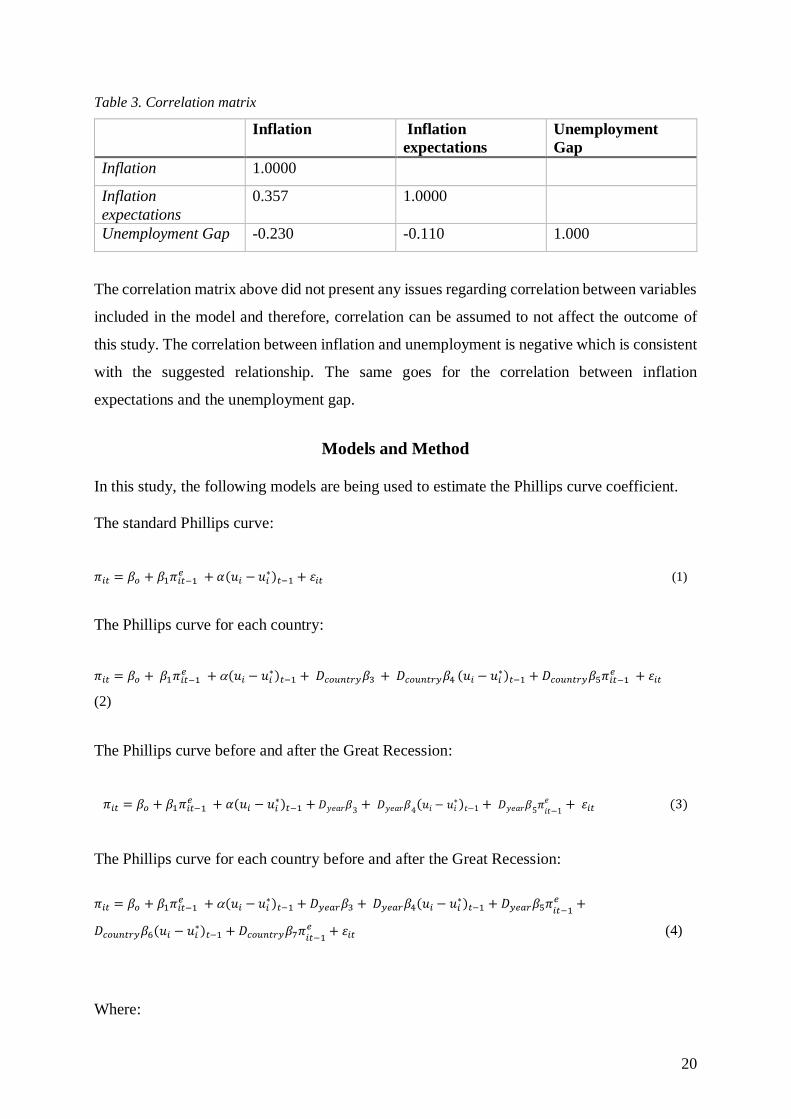
Table 3. Correlation matrix
Inflation Inflation
expectations
Unemployment
Gap
Inflation 1.0000
Inflation
expectations
0.357 1.0000
Unemployment Gap -0.230 -0.110 1.000
The correlation matrix above did not present any issues regarding correlation between variables
included in the model and therefore, correlation can be assumed to not affect the outcome of
this study. The correlation between inflation and unemployment is negative which is consistent
with the suggested relationship. The same goes for the correlation between inflation
expectations and the unemployment gap.
Models and Method
In this study, the following models are being used to estimate the Phillips curve coefficient.
The standard Phillips curve:
𝜋𝑖𝑡 = 𝛽𝑜 + 𝛽1𝜋𝑖𝑡−1𝑒 + 𝛼(𝑢𝑖 − 𝑢𝑖
∗)𝑡−1 + 𝜀𝑖𝑡 (1)
The Phillips curve for each country:
𝜋𝑖𝑡 = 𝛽𝑜 + 𝛽1𝜋𝑖𝑡−1𝑒 + (𝑢𝑖 − 𝑢𝑖
∗)𝑡−1 + 𝐷𝑐𝑜𝑢𝑛𝑡𝑟𝑦𝛽3 + 𝐷𝑐𝑜𝑢𝑛𝑡𝑟𝑦𝛽4 (𝑢𝑖 − 𝑢𝑖∗)𝑡−1 + 𝐷𝑐𝑜𝑢𝑛𝑡𝑟𝑦𝛽5𝜋𝑖𝑡−1
𝑒 + 𝜀𝑖𝑡
(2)
The Phillips curve before and after the Great Recession:
𝜋𝑖𝑡 = 𝛽𝑜 + 𝛽1𝜋𝑖𝑡−1𝑒 + 𝛼(𝑢𝑖 − 𝑢𝑖
∗)𝑡−1 + 𝐷𝑦𝑒𝑎𝑟𝛽3
+ 𝐷𝑦𝑒𝑎𝑟𝛽4(𝑢𝑖 − 𝑢𝑖
∗)𝑡−1 + 𝐷𝑦𝑒𝑎𝑟𝛽5
𝜋 𝑖𝑡−1
𝑒 + 𝜀𝑖𝑡 (3)
The Phillips curve for each country before and after the Great Recession:
𝜋𝑖𝑡 = 𝛽𝑜 + 𝛽1𝜋𝑖𝑡−1𝑒 + (𝑢𝑖 − 𝑢𝑖
∗)𝑡−1 + 𝐷𝑦𝑒𝑎𝑟𝛽3 + 𝐷𝑦𝑒𝑎𝑟𝛽4(𝑢𝑖 − 𝑢𝑖∗)𝑡−1 + 𝐷𝑦𝑒𝑎𝑟𝛽5𝜋
𝑖𝑡−1𝑒 +
𝐷𝑐𝑜𝑢𝑛𝑡𝑟𝑦𝛽6(𝑢𝑖 − 𝑢𝑖∗)𝑡−1 + 𝐷𝑐𝑜𝑢𝑛𝑡𝑟𝑦𝛽7𝜋
𝑖𝑡−1𝑒 + 𝜀𝑖𝑡 (4)
Where:

21
• πit is inflation for country i at time-period t.
• 𝜋𝑖𝑡 𝑒 is representing inflation expectations for country i at time-period t.
• 𝑢𝑖 is the actual unemployment rate for country i.
• 𝑢𝑖∗ represents NAIRU for country i.
• (𝑢𝑖 − 𝑢𝑖∗)𝑡−1 is the unemployment gap at time-period t-1.
• is the Phillips curve coefficient for the reference country.
• 𝐷𝑐𝑜𝑢𝑛𝑡𝑟𝑦 is a dummy variable for each country.
• 𝐷𝑦𝑒𝑎𝑟 is a dummy variable that takes on a value of 0 before 2008 and 1 after 2008.
The first model is used for estimating the average Phillips curve for all countries together.
Model two is used to examine if there exist any country-specific differences in the Phillips
curve. This is done by including an interaction term between the unemployment gap/inflation
expectations and a dummy variables for each country. The country of reference chosen is
Germany. That is because of its size and the key role Bundesbank plays when ECB sets the
monetary policy for the euro area (Alessi, 2013). By including interaction terms between a
dummy variable which captures the crisis and unemployment gap/inflation, model three and
four attempts to explain if the Great Recession had any effect on the relationship.
The statistical method used in this study is Ordinary least squares. A time-series empirical
analysis might be a more accurate method, but due to time limits, the approach mentioned above
will be used.
Problems with endogeneity can occur when estimating the Phillips curve. Endogeneity, also
known as simultaneous causality, which means causality running from the dependent variable
to one or more of the independent variables (Y causes X), instead of running from the
independent variable to the dependent variable (X causes Y). Stock & Watson (2015) states
that having problems with endogeneity will cause the OLS-estimator to be biased and
inconsistent since it picks up both effects. Further, Stock & Watson (2015) mentions two ways
of solving this problem. The first one is the use of lags on the independent variable that is
suspected to cause the simultaneous causality and the second one is to use an instrumental
variable. The method used in this study to address this problem is to include lags on the
independent variables. Several of different lag-length have been tested. The most significant
results was given by including one year’s lag, hence that will be used in the models. By doing

22
this, the unemployment gap will have an effect on inflation but inflation will not affect the
unemployment gap. This implies that (𝑢𝑖 − 𝑢𝑖∗) in time period t affects inflation in time period
t+1. By this, inflation cannot influence the unemployment gap. By including lags in the model,
consideration is also taken to some of the inflation persistence.
Another potential problem that might occur when using panel-data is autocorrelation, which
implies that the error term is correlated with itself over time. Kennedy (2003) points out some
reasons why. It can be due to spatial autocorrelation which happens if random shocks cause
changes in the economic activity in one region and at the same time affect the economic activity
in an adjacent region due to its close economic ties. Random shocks can also affect the
economic activity over more than one time period and this can, therefore, cause autocorrelation.
Another factor that Kennedy (2003) points out is inertia. Inertia refers to past actions having a
significant effect on future economic activities. Furthermore, the smoothing procedures that
many published data have undergone can lead to disturbances over more than one time period
and, therefore, cause autocorrelation. Last but not least, incorrect model-specifications can lead
the error term to be correlated over time if the omitted variable is being autocorrelated.
The data contains 144 observations and therefore, according to the Law of Large Numbers the
large sample size makes the influence of outliers very small (Stock & Watson, 2015). The
sample can be assumed to be approximately normal distributed since the large sample makes
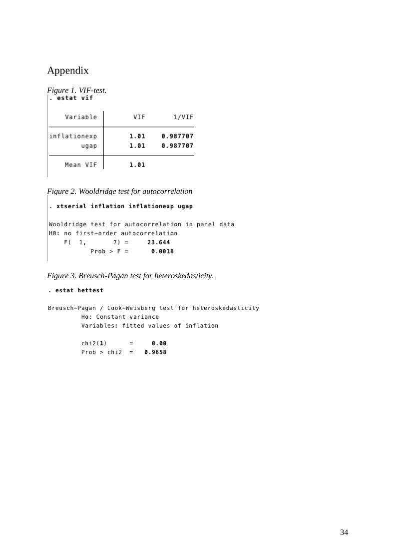
the Central Limit Theorem applicable. A VIF-test has been conducted in order to check for
multicollinearity. A mean value of 1.01 was obtained which implies that there exist no serious
issues with multicollinearity. See appendix figure 1.
A Woolridge test has been performed in order to test the model for autocorrelation (see
appendix figure 2). The result indicated for autocorrelation which has to be taken into account
since that violate against the second ordinary least squares assumption that the error terms have
to be uncorrelated. When having problems with autocorrelation, Ordinary Least Square
estimators will be unbiased. The problem with autocorrelation is solved by using a Generalized
Least Square estimator. Generalized Least Square helps to estimate the unknown parameter
when there exist a certain degree of correlation between the error term in a linear regression
model (Stock & Watson, 2015). To check for heteroskedasticity, a Breusch-Pagan test has been
performed where the result implied that there exists no heteroskedasticity (see appendix figure
3).

23
5. Result
First of all, the Phillips curve coefficient is presented. Later on, the Phillips curve coefficient
for each country will be presented. At last, estimations on how the Great Recession has
affected the relationship are being presented.
The standard Phillips curve
𝜋𝑖𝑡 = 𝛽𝑜 + 𝛽1𝜋𝑖𝑡−1𝑒 + 𝛼(𝑢𝑖 − 𝑢𝑖
∗)𝑡−1 + 𝜀𝑖𝑡 (1)
Table 5. Estimating the Phillips curve coefficient.
Coefficient
Standard
Error Z-value P-value 95% Confidence Interval
Inflation
expectations
0.038
0.086 0.45 0.656 -0.130 0.207
Unemployment
gap
-0.131**
0.066 -1.99 0.047 -0.260 -0.001
Constant 1.566*** 0.167 0.000 0.000 1.237 1.895
Wald chi (2) = 4.39
Probability > chi2 = 0.111 Number of observation: 136.
***,**,* corresponds to 1%, 5%, 10% significant level.
As shown in Table 5 above, the result shows that there exist, on average, a negative relationship
between inflation- and the unemployment rate. A result which is statistically significant on a 5
% level. This is expected and also in line with what the theory behind the Phillips curve states.
However, the results did not present any statistical evidence that inflation expectations have
any effect on inflation.
The Phillips curve for each country
𝜋𝑖𝑡 = 𝛽𝑜 + 𝛽1𝜋𝑖𝑡−1𝑒 + (𝑢𝑖 − 𝑢𝑖
∗)𝑡−1 + 𝐷𝑐𝑜𝑢𝑛𝑡𝑟𝑦𝛽3 + 𝐷𝑐𝑜𝑢𝑛𝑡𝑟𝑦𝛽4 (𝑢𝑖 − 𝑢𝑖∗)𝑡−1 + 𝐷𝑐𝑜𝑢𝑛𝑡𝑟𝑦𝛽5𝜋𝑖𝑡−1
𝑒 (2)
As the empirical test is being made with Germany as the reference country, the coefficient for
the unemployment gap shows the difference in the slope of the Phillis curve between Germany
and a given country. The slope of the Phillips curve for each country is obtained by adding ,

24
with the difference in the slope of the Phillips curve between Germany and each of the given
countries, 𝛽3. An increase in the unemployment gap indicates that the actual unemployment is
higher than its natural rate.
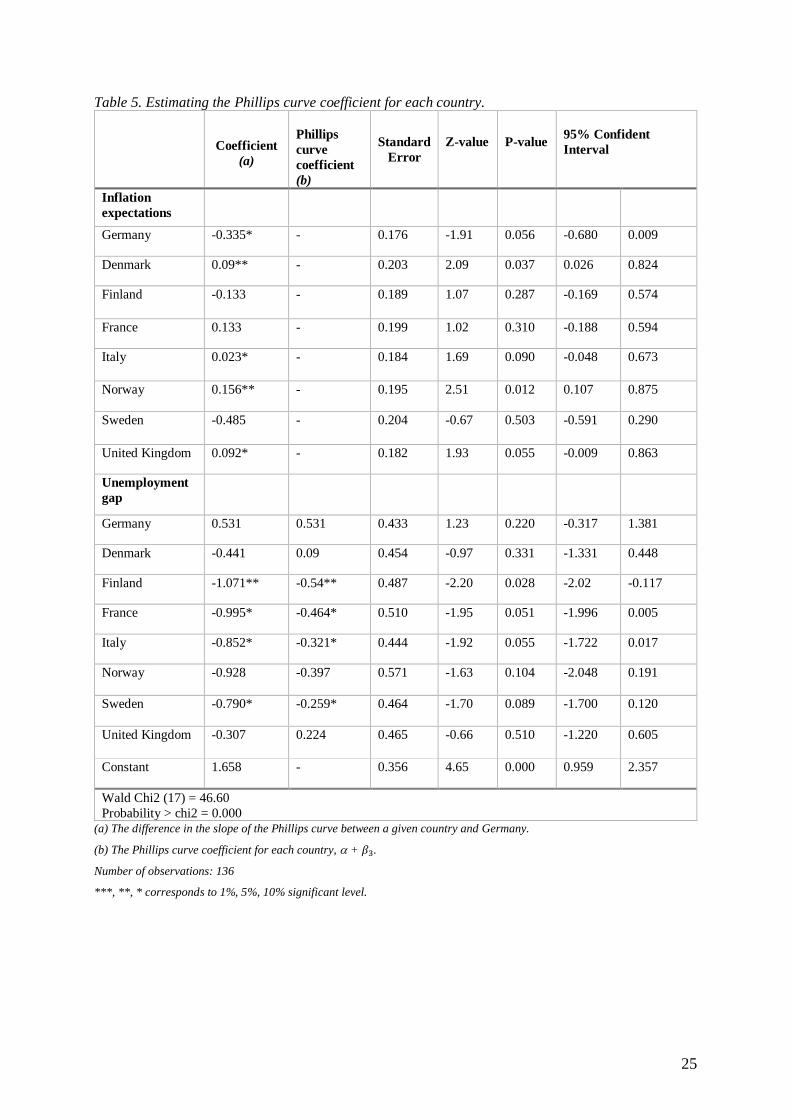
The results, presented in Table 5, shows significant country-specific differences in the slope of
the Phillips curve between Finland and Germany. Further, the results indicate that there exist
country-specific differences between Germany and Italy, France and Sweden, although, that
result is only significant at 10 %.
The results also show a significant negative relationship between the unemployment rate and
inflation in Finland. The same goes for France, Italy and, Sweden but this is only significant at
10% level. Although, as the confidence interval lies between -1.996 and 0.005 for France, -
1.722 and 0.017 for Italy and -1.700 and 0.120 for Sweden, the probability that the coefficient
would take a positive value in these countries is rather small. In Finland where one percentage
point increase in unemployment gap will lead the inflation to fall with 0.54 percentages point,
which also makes Finland the country where changes in the unemployment rate have the most
powerful effect on inflation. The relationship is weakest in Sweden where one percentages point
increase in the unemployment gap will have a decreasing effect on inflation with 0.259
percentages point. However, there is no statistical evidence that there exist any country-specific
differences in the slope of the Phillips curve between Germany and the other countries namely
Norway, Denmark, and the United Kingdom.
In Norway and Denmark inflation expectations is significant on a 5 % level, while inflation
expectations are significant on a 10% level in Germany, Italy and, the United Kingdom. What
one could find remarkable is that the coefficient for Germany takes on a negative value, which
contradicts what theory states. Italy is the only country where both inflation expectations and
the unemployment gap affects inflation. For the rest of the countries, it is either the
unemployment gap or inflation expectations that have a significant effect on inflation.
25
Table 5. Estimating the Phillips curve coefficient for each country.
Coefficient
(a)
Phillips
curve
coefficient
(b)
Standard
Error
Z-value
P-value
95% Confident
Interval
Inflation
expectations
Germany -0.335*
- 0.176 -1.91 0.056 -0.680 0.009
Denmark 0.09**
- 0.203 2.09 0.037 0.026 0.824
Finland -0.133
- 0.189 1.07 0.287 -0.169 0.574
France 0.133
- 0.199 1.02 0.310 -0.188 0.594
Italy 0.023*
- 0.184 1.69 0.090 -0.048 0.673
Norway 0.156**
- 0.195 2.51 0.012 0.107 0.875
Sweden -0.485
- 0.204 -0.67 0.503 -0.591 0.290
United Kingdom 0.092*
- 0.182 1.93 0.055 -0.009 0.863
Unemployment
gap
Germany 0.531
0.531 0.433 1.23 0.220 -0.317 1.381
Denmark -0.441
0.09 0.454 -0.97 0.331 -1.331 0.448
Finland -1.071**
-0.54** 0.487 -2.20 0.028 -2.02 -0.117
France -0.995*
-0.464* 0.510 -1.95 0.051 -1.996 0.005
Italy -0.852*
-0.321* 0.444 -1.92 0.055 -1.722 0.017
Norway -0.928
-0.397 0.571 -1.63 0.104 -2.048 0.191
Sweden -0.790*
-0.259* 0.464 -1.70 0.089 -1.700 0.120
United Kingdom -0.307
0.224 0.465 -0.66 0.510 -1.220 0.605
Constant 1.658
- 0.356 4.65 0.000 0.959 2.357
Wald Chi2 (17) = 46.60
Probability > chi2 = 0.000 (a) The difference in the slope of the Phillips curve between a given country and Germany.
(b) The Phillips curve coefficient for each country, + 𝛽3.
Number of observations: 136
***, **, * corresponds to 1%, 5%, 10% significant level.

26
The Phillips curve before and after the Great Recession.
𝜋𝑖𝑡 = 𝛽𝑜 + 𝛽1𝜋𝑖𝑡−1𝑒 + 𝛼(𝑢𝑖 − 𝑢𝑖
∗)𝑡−1 + 𝐷𝑦𝑒𝑎𝑟𝛽3
+ 𝐷𝑦𝑒𝑎𝑟𝛽4(𝑢𝑖 − 𝑢𝑖
∗)𝑡−1 + 𝐷𝑦𝑒𝑎𝑟𝛽5
𝜋 𝑖𝑡−1
𝑒 + 𝜀𝑖𝑡 (3)
In order to see if the crisis had any effect on the Phillips curve, interaction terms between
unemployment gap/inflation expectations and a dummy have been included in the model. As
the dummy variable takes on a value of zero before 2008 and 1 after 2008, the coefficient for
the unemployment gap after the crisis is obtained by adding 𝛼 and 𝛽4. Whereas the coefficient
for inflation expectations is obtained by adding 𝛽1 and 𝛽5. The results, presented in Table 6,
shows that the Great Recessions did not have any significant effect on either the
unemployment gap or inflation expectations.
Table 6. Estimating the Phillips curve coefficient before and after the Great Recession.
Coefficient Standard
Error Z-value P-value 95% Confident Interval
Inflation
Expectations
Before
After
0.0232
0.044
0.174
0.099
0.13
0.45
0.894
0.651
-0.318
-0.149
0.365
-0.239
Unemployment
Gap
Before
After
-0.116
-0.124
0.110
0.084
-1.05
-1.48
0.292
0.139
-0.333
-0.290
0.100
0.040
Constant 1.690*** 0.319 5.30 0.000 1.065 2.316
Wald chi (4) = 5.09
Probability > chi2 = 0.278 Number of observations:136
*, **, *** corresponds to 1%, 5%, 10% significant level.
The Phillips curve for every country before and after the Great Recession
𝜋𝑖𝑡 = 𝛽𝑜 + 𝛽1𝜋𝑖𝑡−1
𝑒 + (𝑢𝑖 − 𝑢𝑖∗)𝑡−1 + 𝐷𝑦𝑒𝑎𝑟𝛽3 + 𝐷𝑐𝑜𝑢𝑛𝑡𝑟𝑦𝛽4 + 𝐷𝑐𝑜𝑢𝑛𝑡𝑟𝑦𝛽5(𝑢𝑖 − 𝑢𝑖
∗)𝑡−1 + 𝐷𝑐𝑜𝑢𝑛𝑡𝑟𝑦𝛽6𝜋 𝑖𝑡−1𝑒 +
𝐷𝑦𝑒𝑎𝑟(𝐷𝑐𝑜𝑢𝑛𝑡𝑟𝑦𝛽7(𝑢𝑖 − 𝑢𝑖∗)𝑡−1) + 𝐷𝑦𝑒𝑎𝑟(𝐷𝑐𝑜𝑢𝑛𝑡𝑟𝑦𝛽8𝜋
𝑖𝑡−1𝑒 ) + 𝜀𝑖𝑡 (4)
In model 4, new variables has been generated, 𝐷𝑐𝑜𝑢𝑛𝑡𝑟𝑦𝛽4(𝑢𝑖 − 𝑢𝑖∗)𝑡−1 and 𝐷𝑐𝑜𝑢𝑛𝑡𝑟𝑦 𝛽5𝜋
𝑖𝑡−1𝑒 . Those
variables capture inflation expectations and the unemployment gap for each specific country.
So, in order to see how the crisis did affect the Phillips curve, a dummy variable which captures
the crisis has been interacted with the country-specific variables for the unemployment gap and
inflation expectations.

27
The result, presented in Table 7, shows that it exist no statistical relationship between the
unemployment gap and inflation in none of the countries before the crisis except in Finland.
After the crisis, inflation have become less sensitive to changes in the unemployment gap in
Finland, which is statistical significant on 5 %. As mentioned above, this study reveals that
there exist no relationship between the unemployment gap and inflation in Italy and France, but
after the crisis, we can see that the relationship becomes negative and significant on 5%
respective 10%. For the rest of the countries, no evidence where found that the crisis had any
effect on the Phillips curve. Germany and Sweden are the only countries where the crisis had
an effect on inflation expectations.
Table 7. Estimating the Phillips curve coefficient for every country before and after the Great Recession.
Coefficient Standard
Error Z-value P-value
95% Confidence
Interval
Inflation
expectations
Germany
Before
After
-0.345
-0.382*
0.362
0.196
-0.95
-1.94
0.340
0.052
-1.056
-0.768
0.364
0.003
Denmark
Before
After
-0.138
0.031
0.286
0.153
-0.48
0.20
0.629
0.840
-0.700
-0.270
0.423
0.332
Finland
Before
After
0.032
-0.219
0.271
0.135
0.12
-1.62
0.904
0.106
-0.498
-0.486
0.564
0.046
France
Before
After
-0.065
-0.288
0.253
0.189
-0.26
-1.52
0.795
0.128
-0.563
-0.659
0.431
0.083
Italy
Before
After
0.179
-0.071
0.221
0.147
0.81
-0.48
0.418
0.630
-0.255
-0.360
0.613
0.218
Norway
Before
After
0.021
-0.071
0.221
0.147
0.81
-0.48
0.418
0.630
-0.255
-0.360
0.613
0.218
Sweden
Before
After
-0.829**
-0.394**
0.414
0.164
-2.00
-2.40
0.046
0.017
-1.642
-0.716
-0.016
-0.071
United
Kingdom
Before
After
0.010
0.127
0.386
0.136
0.03
0.93
0.979
0.353
-0.746
-0.141
0.766
0.395
Unemployment
gap
Germany
Before
After
0.276
1.553
0.544
1.324
0.51
1.17
0.612
0.241
-0.789
-1.042
1.342
4.150

28
Denmark
Before
After
-0.392
0.123
0.601
0.133
-0.65
0.93
0.514
0.354
-1.571
-0.137
0.785
0.384
Finland
Before
After
-0.803**
-0.691**
0.384
0.334
-2.09
-2.06
0.037
0.039
-1.557
-1.347
-0.049
-0.035
France
Before
After
-0.182
-0.548*
0.600
0.291
-0.30
-1.88
0.761
0.060
-1.358
-1.120
0.993
0.023
Italy
Before
After
0.069
-0.404***
0.205
0.115
0.34
-3.49
0.736
0.000
-0.332
-0.631
0.471
-0.177
Norway
Before
After
-0.470
-0.271
0.575
0.497
-0.82
-0.55
0.414
0.585
-1.598
-1.245
0.657
0.703
Sweden
Before
After
-0.417
-0.325
0.303
0.371
-1.38
-0.88
0.168
0.380
-1.011
-1.053
0.176
0.402
United
Kingdom
Before
After
0.191
0.233
0.420
0.240
0.46
1.18
0.629
0.840
-0.700
-0.270
0.423
0.332
Constant 1.943*** 0.330 5.88 0.000 1.295 2.590
Chi2 (33) = 64.11
Probability > chi2 =0.000 Number of observations: 136
*, **, *** corresponds to 1%, 5%, 10% significant level.

29
6. Discussion
The aim of this study was to investigate the slope of the Phillips curve in eight advanced
economies. Based on previous findings from Ball and Mazumder (2014) and Simon et al.,
(2013), this study further aimed to examine whether the Great Recession had any impact on the
slope of the Phillips curve. However, this study has been made with slightly different models
compare to models used by researchers in previous studies. The most significant difference is
that Simon et al., (2013) are including import prices which aims to take into account that global
factors affect domestic inflation. They also included a variable that captures supply shocks.
Unfortunately, data over import prices and supply shocks were not available and is, therefore,
the reason why those variables are not included in the models used in this study.
The result showed that there exist country-specific differences between countries that are part
of the eurozone, namely France, Italy, Finland, and Germany. As ECB, however, treats these
countries with one single monetary policy. Such heterogeneity among these countries can lead
the same monetary policy to have different outcomes in each country. That is something that
policymakers is needed to be aware of (ECB, 2011).
Can the country specific differences in institutions on the labor market describe why countries
face different slopes in the Phillips curve? Adamo & Rovelli (2013) have found that in countries
where the expenditure on labor market policies is high, inflation is less sensitive for changes in
the unemployment rate. In countries where the role of labor market institutions are limited,
inflation is more responsive for changes in unemployment. The findings from Adamo & Rovelli
(2013) goes in line with findings in this study when it comes to Sweden. Sweden faces the
weakest relationship between inflation and the unemployment rate and it is also the country
where the expenditure on the labor market is one of the highest among the countries in Europe
(European Parliament, 1997). However, according to Schindler (2014), Italy faces one of the
worst performing labor market institutions in EU which should, according to the findings in
Adamo & Rovelli (2013) study, yield a strong trade-off between inflation and unemployment.
Although, the results from this study implies the opposite, as Italy faces the weakest trade-off
among the countries where the results were significant. Sweden, however, has one of the highest
rate of union memberships in Europe (Forbes, 2017). The aim of this study was not to examine
the impact of labor market institutions on the slope of the Phillips curve, but for further studies,
a relevant question to analyze would be how the set of labor market institutions actually affects

30
the slope of the Phillips curve and if those can explain why countries face different slopes in
the Phillips curve.
As mentioned in the results, the Great Recession had an steepening effect on the Phillips curve
in Italy and France. That indicates that inflation is more sensitive to changes in unemployment.
For Italy and France, the results also goes in line with what Bulligan & Vivano ( 2016) found
in their study. So, what can be the explanation to why inflation had become more sensitive to
changes in unemployment? It is hard to determine the actual reason for the steepening Phillips
curve in these countries as more specific studies on how France and Finland was affected by
the crisis. But potential explanations for a steepening Phillips curve can be changes in the wage-
setting behavior by firms, a factor that Bulligan & Vivano (2016) also mentions. On the other
hand, it might be possible that during these kinds of crisis, workers and unions will accept a
lager cut in wages in order to be able to still keep their jobs. Which will make wages more
sensitive to economic slack. Another possible explanation to a steeper Phillips curve can also
be changes in the labor market institutions that have provided less rigidities. Last but not least,
the correlation between inflation and unemployment is affected by other underlying factors and
how strong the correlation is between inflation and unemployment will depend on how these
other factors behave relative to each other. So, even though it seems like the relationship have
become stronger, the actual reason for that can be that the underlying factors are behaving
differently. To determine the actual reason for the steepening curve, further studies on the labor
market in France and Italy is needed. The crisis had a weakening effect on the slope of the
Phillips curve in Finland. As many other countries in Europe, Finland faced an increase in
unemployment after the crisis (Järvinen & Laitamäki, 2013). Potential explanations for this
change can be that NAIRU increased as people who became unemployed turned in to being
long-term unemployed. It can also be due do that inflation expectations have become more
anchored. As in the case with France and Italy, further studies on how the crisis did affect the
labor market and the behavior of inflation in Finland is needed to be able to point out the actual
reason for this change.
For Finland, France, Italy and Sweden, evidence shows that there exist a correlation we can say
that the Phillips curve could still be alive and well. As the results did not present any statistical
evidence for a correlation between inflation and unemployment in Germany, Norway and the
United Kingdome it is not possible for study to prove for an existing Phillips curve. Although,
future studies is needed to be made and consideration should be given to other variables that

31
affect inflation, for example, globalization, supply shocks, or more anchored inflation
expectations. Further studies should also focus on how/if price and wage rigidities has changes
after the crisis as that can lead inflation to be less sensitive to changes in unemployment.
32
Reference list
Alessi, C. (2013) Germany’s Central Bank and the Eurozone. Council on Foreign Relations.
Retrieved from: https://www.cfr.org/backgrounder/germanys-central-bank-and-eurozone
Ball, L. M., & Mankiw, N. G. G. (2002). The NAIRU in Theory and Practice. Journal of
Economic Perspectives, 16(4), 115–136. https://doi.org/10.2139/ssrn.319703
Ball, L. M., & Mazumder, S. (2011). Inflation Dynamics and the Great Recession. SSRN
Electronic Journal. https://doi.org/10.2139/ssrn.1833648
Ball, L., & Mazumder, S. (2014). A Phillips Curve with Anchored Expectations and Short-
Term Unemployment. https://doi.org/10.3386/w20715
Bergstr, V., & Boije, R. (2005). Penningpolitik och arbetslöshet. Sveriges Riksbank, 4/2005,
15-49.
Bhattarai, K. (2016). Unemployment – inflation trade-offs in OECD countries. Economic
Modelling, 58, 93–103. https://doi.org/10.1016/j.econmod.2016.05.007
Binder, C. C. (2016). Comment: “Is the Phillips Curve Alive and Well after All? Inflation
Expectations and the Missing Disinflation.” SSRN Electronic Journal, 7, 197–232.
https://doi.org/10.2139/ssrn.2789901
Blanchard, O., Amighini, A., & Giavazzi, F. (2017). Macroeconomics: A European
Perspective. https://doi.org/10.1007/s13398-014-0173-7.2
Blanchard, O., & Wolfers, J. (2000). The Role of Shocks and Institutions in the Rise of
European Unemployment : The Aggregate Evidence. The Economic Journal, 110.
Bowdler, C., & Nunziata, L. (2005). Trade Union Density and Inflation Performance:
Evidence from OECD Panel Data. Economica, 74(293), 135–159.
https://doi.org/10.1111/j.1468-0335.2006.00532.x
Bullard, J. (2016). Inflation Expectations Are Important to Central Bankers, Too. Federal
Reserve Bank of St. Louis, 2016.
Bulligan, G., & Vivano, E. (2016). Has the wage Phillips curve changed in the euro area?
https://doi.org/10.1016/j.econlet.2016.06.031
Bulligan, G., & Viviano, E. (2017). Has the wage Phillips curve changed in the euro area?
IZA Journal of Labor Policy, 6(1). https://doi.org/10.1186/s40173-017-0087-z
D’Adamo, G., & Rovelli, R. (2013). Labor Market Institutions and the Response of Inflation
to Macro Shocks in the EU: A Two-Sector Analysis, (7616). Retrieved from
http://ftp.iza.org/dp7616.pdf
ECB. (2011). The Monetary Policy of the ECB 2011. The European Central Bank, 2011.

33
Gordon, R. (2013). The Phillips Curve is Alive and Well: Inflation and the NAIRU During
the Slow Recovery. National Bureau of Economic Research (Vol. w19390). Cambridge,
MA. https://doi.org/10.3386/w19390
European Parliament. (1997) Social and Labour Market Policy in Sweden. Retrieved from:
http://www.europarl.europa.eu/workingpapers/soci/w13/summary_en.htm
Hong, G. H., Koczan, Z., Lian, W., & Nabar, M. (2018). More Slack than Meets the Eye?
Recent Wage Dynamics in Advanced Economies. IMF Working Papers (Vol. 18).
https://doi.org/10.5089/9781484345351.001
Iakova, D. M. (2007). Flattening of the Phillips Curve: Implications for Monetary Policy. IMF
Working Papers, 07(76), 1. https://doi.org/10.5089/9781451866407.001
Järvinen, R., & Laitamäki, J. (2013). The Impact of the 2008 Financial Crises on Finnish and
American Households. LTA, 13(1), 41–65. Retrieved from
http://njb.fi.s189994.gridserver.com/wp-
content/uploads/2015/04/2013_1_Paper_Laitamaki_Jarvinen.pdf
Karlsson, S., & Österholm, P. (2018). A Note on the Stability of the Swedish Philips Curve.
School of Business, Örebro Univeristy.
Kennedy, P. (2003). A guide to econometrics (Vol. 5th). https://doi.org/10.1016/0164-
0704(93)90038-N
OECD. (2017) Harmonised Unemployment rate.
https://data.oecd.org/unemp/harmonised-unemployment-rate-hur.htm
Phelps, E. (1967). Phillips Curves , Expectations of Inflation and Optimal Unemployment
over Time Author, 34(135), 254–281.
Samuelson, P. A., & Solow, R. M. (1960). Analytical Aspects of Anti-Inflation Policy., 50(2).
Schindler, M. (2014). The Italian Labor Market: Recent Trends, Institutions, and Reform
Options. IMF Working Papers, 09(47), 1. https://doi.org/10.5089/9781451871951.001
Simon, J., Matheson, T., & Sandri, D. (2013). The Dog That Didn’t Bark: Has Inflation Been
Muzzled or Was It Just Sleeping? International Monetary Fund.
https://doi.org/http://dx.doi.org/10.1016/j.biombioe.2014.10.011
Stock, J. H., & Watson, M. W. (2015). Introduction to Econometrics.
https://doi.org/10.1093/acprof
Sveriges Riksbank. (2016). Penningpolitisk rapport december 2016.
The Economist. (2017, 1 November) The Phillips curve may be broken for good. Retrieved
from:https://www.economist.com/graphic-detail/2017/11/01/the-phillips-curve-may-be-
broken-for-good
34
Appendix
Figure 1. VIF-test.
Figure 2. Wooldridge test for autocorrelation
Figure 3. Breusch-Pagan test for heteroskedasticity.