Policy Research Working Paper 8362

The Performance of a Consumption Augmented Asset Index in Ranking

Households and Identifying the PoorDiana Ngo

Luc Christiaensen

Social Protection and Labor Global PracticeMarch 2018

WPS8362P

ublic

Dis

clos

ure

Aut

horiz

edP

ublic

Dis

clos

ure

Aut

horiz

edP

ublic

Dis

clos

ure

Aut

horiz

edP

ublic

Dis

clos

ure

Aut

horiz

ed

Produced by the Research Support Team

Abstract

The Policy Research Working Paper Series disseminates the findings of work in progress to encourage the exchange of ideas about development issues. An objective of the series is to get the findings out quickly, even if the presentations are less than fully polished. The papers carry the names of the authors and should be cited accordingly. The findings, interpretations, and conclusions expressed in this paper are entirely those of the authors. They do not necessarily represent the views of the International Bank for Reconstruction and Development/World Bank and its affiliated organizations, or those of the Executive Directors of the World Bank or the governments they represent.

Policy Research Working Paper 8362

This paper is a product of the Social Protection and Labor Global Practice. It is part of a larger effort by the World Bank to provide open access to its research and make a contribution to development policy discussions around the world. Policy Research Working Papers are also posted on the Web at http://econ.worldbank.org. The authors may be contacted at lchristiaensen@worldbank.org.

Asset ownership indices are widely used as inexpensive prox-ies for consumption. This paper shows that these indices can be augmented using dichotomous indicators for con-sumption, which are equally easy to obtain. The paper uses multiple rounds of Living Standards Measurement Study surveys from Malawi, Uganda, Rwanda, Tanzania, and Ghana to construct indices with different item subcatego-ries and performs a meta-analysis comparing the indices to per capita consumption. The results show that the standard asset indices, which are derived from durable ownership and

housing characteristic indicators, perform well in urban settings. Yet, in rural samples and when identifying the extreme poor, household rankings and poverty classification accuracy can be meaningfully improved by adding indi-cators of food and semi-durable consumption. The study finds small improvement from using national weights in urban samples but no improvement from using alterna-tive construction methods. With most of Africa’s poor concentrated in rural areas, these are important insights.

The Performance of a Consumption Augmented Asset Index

in Ranking Households and Identifying the Poor

Diana Ngo and Luc Christiaensen1

JEL Codes: I32, O10.

Keywords: asset index, poverty targeting, consumption proxies, proxy-means testing.

                                                            1 Diana Ngo (dngo@oxy.edu) is Assistant Professor at Occidental College. Luc Christiaensen is Lead Economist at the Jobs Group of the World Bank. The findings, interpretations, and conclusions expressed in this paper are entirely those of the authors. They do not necessarily represent the views of the International Bank for Reconstruction and Development/World Bank and its affiliated organizations, or those of the Executive Directors of the World Bank or the governments they represent.

2  

1 Introduction

The state of poverty is commonly assessed in monetary terms using information on household consumption

expenditures and auxiliary data on prices (Deaton, 2006; Ravallion, 2015; World Bank, 2015).2 However,

frequent, reliable, and comparable information on consumption and prices is often hard to come by,

especially in developing countries (Beegle et al., 2016). This has spawned a buoyant search for less costly

alternatives to identify and target poor people (Sahn and Stifel, 2003; Rutstein and Johnson, 2004), to track

progress on poverty (Sahn and Stifel, 2000; Christiaensen et al., 2012; Rutstein and Staveteig, 2014), or

simply to control for or make inferences about the effect of socio-economic status (SES) and poverty on

non-monetary indicators of well-being such as education and health (Howe et al., 2009; Filmer and Scott,

2012).

These alternative indices are typically constructed from dichotomous indicators of asset ownership and

housing characteristics (e.g., sanitation, electricity, and quality of floors). This makes them less demanding

and less costly in terms of data collection and less prone to measurement error (Sahn and Stifel, 2003;

Maitra, 2016). Weights are then derived to combine the indicators into a unitary asset index. Statistical

asset indices derive weights from the statistical relations between the indicators and do not require any

information on consumption.3 Principal components and factor analysis are frequently used to do so,

whereby the coefficients on the first component or factor are used as weights (Filmer and Pritchett, 2001;

Sahn and Stifel, 2003; Rutstein and Johnson, 2004). However, other methods have also been proposed and

validated. These include inverse frequency weighting (Morris et al., 2000) and threshold or item response

models, which are based on the notion that the observed presence of an asset is linked to unobserved wealth

(Ferguson et al. 2003; Baker and Kim, 2004; Maitra, 2016).

                                                            2 For example, the first indicator of UN Sustainable Development Goal I “Ending Poverty” is “Eradicating extreme poverty for all people everywhere,” measured as “people living on less than $1.25 a day.” (http://www.un.org/sustainabledevelopment/poverty/). Recently, non-monetary and multi-dimensional measures of poverty are often reported in conjunction (Ferreira and Lugo, 2013; Alkire and Santos, 2014; Beegle et al., 2016). 3 There is also a class of “economic” asset indices that derive weights by regressing expenditure on the indicator variables (Stifel and Christiaensen, 2007). Applications include the Simple Poverty Scorecard developed by Mark Schreiner of Microfinance Risk Management, L.L.C, which has been widely used among microfinance institutions, NGOs, and agribusiness companies targeting the poor and the Survey of Well-Being via Instant and Frequent Tracking developed by Nobuo Yoshida of the World Bank (https://collaboration.worldbank.org/docs/DOC-15061). Economic asset indices have the appeal of generating weights that can be interpreted as economic returns (Christiaensen et al., 2012; Douidich et al., 2015; Beegle et al., 2016). However, they cannot be estimated without some initial information on the consumption behavior of the study population. Relatedly, Ngo (2018) develops an asset index that does not require information on consumption, but it does require additional information on asset prices. These indices are therefore more demanding in terms of data requirements and not available in as many settings relative to statistical asset indices. The remainder of the paper concerns only statistical asset indices, which we simply refer to as “asset indices.” 

3  

Asset indices have commonly been used to proxy for SES across a range of academic fields. They have

been used in studies on education (Acham et al., 2012), the environment (Holmes, 2003; Caldas et al.,

2007), and economics (Gunning et al., 2000; Simmons et al., 2009). They are also widely used in research

on health determinants and inequalities (Wagstaff and Watanabe, 2003; Howe, Hargreaves and Huttly,

2008; Howe et al., 2009). Various studies report that, compared with measures of consumption, asset

indices yield similar inferences about the extent to which inequalities in education, health, and fertility are

related to SES (Morris et al., 2000; Filmer and Pritchett, 2001; Ferguson et al., 2003; Montgomery and

Hewett, 2005; Filmer and Scott, 2012). Asset indices are also used in proxy means testing to target poor

households for program support and have been shown to perform reasonably well in various settings

(Coady, Grosh, and Hoddinott, 2004; Gwatkin, Wagstaff, and Yazbeck, 2005; Handa and Davis, 2006).

Despite their common usage, asset indices still have some important limitations. First, many asset indices

have problems with clumping. They are often unable to distinguish among the poorest households, which

do not own any of the included durables and housing variables (McKenzie, 2005; Vyas and Kumaranayake,

2006). This concern is particularly large in rural areas, making it difficult to target programs to poor

households. For example, according to the Living Standards Measurement Studies, only 38 and 52 percent

of the rural population own the most common durable good in Nicaragua in 1998 and in Malawi in 2004,

respectively (Ngo, 2018). Thus, while asset indices work well on average for identifying poor households,

there is considerable variation in targeting performance (Coady, Grosh, and Hoddinott, 2004), and they

tend to be less accurate at lower poverty lines (Handa and Davis, 2006).

Second, researchers and policy makers are often directly interested in household consumption. It is the

traditional metric to measure poverty and capture welfare (Meyer and Sullivan, 2003). While asset indices

have been shown to be correlated with consumption, they typically do not yield the same ranking of

households (Filmer and Scott, 2012). In some contexts, the correlation between asset indices and

consumption is in fact low to moderate at best (Ngo, 2018), leading some researchers to conclude that they

are poor proxies for consumption (Howe et al., 2009). Thus, when household consumption is the goal,

asset indices may induce mistargeting of programs or may generate inaccurate conclusions regarding

inequality (Houweling, Kunst, and Mackenbach, 2003; Lindelow, 2006; Wittenberg and Leibbrandt, 2017).

In this paper, we explore whether the correspondence between asset indices and consumption can be

improved by using different combinations of items that also include indicators for consumption of semi-

durables, staple foods, and non-staple foods. Intuitively, these items may increase the ability to discriminate

among the poorest households if the demand for these goods is highly income elastic at the lower end of

4  

the distribution. The current practice of limiting the set of asset indicators to durables and housing

characteristics has been largely motivated by the ready availability of this information in the Demographic

and Health Surveys and not necessarily by strong theoretical reasons (Rutstein and Johnson, 2004; Gwatkin

et al., 2007). Yet, there is little extra cost to expanding the information base with a limited number of

yes/no questions that capture consumption of a series of food and semi-durable items. For example,

questionnaires could be augmented by including questions such as “Did your household purchase any

clothing in the past year?”

We examine the possibility of including consumption indicators in various contexts and test their

performance using several criteria. This is important because these indices are applied across a range of

settings with different intended applications. As Diamond et al. (2016) highlight in their performance

analysis of the Simple Poverty Score card, which applies the same nationally derived weights across settings

within a country, performance consistency across settings cannot be assumed. Similarly, but even less

commented on in the literature, is heterogeneity in prediction accuracy depending on the poverty level.

Indicator combinations that perform well in identifying the extreme poor are not necessarily also powerful

at identifying the moderate poor, and vice versa.

Specifically, we use 13 surveys from the Living Standards Measurement Studies (LSMS) conducted at

different times in Malawi, Uganda, Rwanda, Tanzania, and Ghana, and we systematically assess the

performance of different indices in ranking households and classifying households as poor/non-poor within

each sample. To do this, we generate indices using 27 different combinations of housing characteristics,

durables, semi-durables, staple foods, and non-staple foods, using between 5 and 27 indicators in total for

each combination.

For each combination, we use three methods to derive individual indicator weights, which differ in their

intuitive appeal and implementation complexity. We then construct the indices within each sample

separately and test how well they correspond to consumption, again within each sample, using rank

correlation coefficients and accuracy measures for identifying both the extreme and moderate poor, using

the 10th and 40th percentile index scores as cutoffs, respectively.4 We do this for national, urban, and rural

samples and also compare the difference in performance when using nationally generated weights as

opposed to rural- and urban-specific weights. We limit our analysis of the performance of these indices to

comparisons within cross-sections, leaving applications to inter-temporal comparisons to future work.

                                                            4 The 40th percentile is the cut-off chosen by the World Bank for its shared prosperity indicator.

5  

Together, this yields a total of 5,265 permutations of variable combinations, construction methods, and

samples. We perform a meta-analysis regression to examine whether the performance of currently popular

sets of asset indices and construction methods can be improved upon, and if so, through which indicator

combination and construction method, in which geographical settings (national, rural, urban), and in which

poverty contexts (extreme, moderate). Overall, the results confirm that the commonly used asset indices,

consisting of indicators for the possession of durable assets and housing characteristics (about 15-20

indicator variables in total) and constructed using principal components analysis, can be effectively used as

proxies for consumption (McKenzie, 2003; Filmer and Scott, 2012).

Yet, the results also show that when it comes to rural settings where the poor tend to be concentrated and

when identifying the extreme poor, both in rural and national samples, performance can be improved at

little extra cost by restricting the standard index (durable asset possessions and housing characteristics) to

a subset of durable indicators (reflecting the five most common durables) and expanding the information

base with a small set of indicator variables capturing the consumption of semi-durables and food. This

consumption augmented asset index (consisting of only 5-10 more indicator variables—25 in total),

increases the targeting accuracy in reaching the extreme poor on average by more than 10 percentage points.

It also increases the rank correlation with consumption among rural households by 9 percentage points.

Among urban samples, the augmented index offers no improvement over the standard asset index, and

nationally generated weights tend to work slightly better.

The paper proceeds as follows. Section 2 motivates the use of consumption as the benchmark and the use

of assets as a proxy. Section 3 introduces the data and discusses the procedure for generating the index

permutations, the performance criteria, and the analytical strategy for the meta-analysis. Section 4 presents

the findings, and Section 5 concludes.

2 Assets and Consumption 

According to the 2001 World Development Report, “Consumption is conventionally viewed as the

preferred welfare indicator, for practical reasons of reliability and because consumption is thought to better

capture long-run welfare levels than current income.” (World Bank, 2001, p.17). This still holds today,

even though the multi-dimensional aspects of poverty are increasingly being recognized (Alkire and Santos,

2014) and SES is at times used instead of consumption (Sahn and Stifel, 2000; Bader et al., 2017).5 In using

consumption as the benchmark, we follow the majority of the asset index literature, which developed and

                                                            5 See Beegle et al. (2016) for a discussion of the conceptual deficiencies in doing so. 

6  

validated the methods against consumption (Morris et al., 2000; Filmer and Pritchett, 2001; Ferguson et al.,

2003).

Measures of consumption are based on current household expenditures (monetary outflow) and derived

following various adjustments. Specifically, outlays on durable goods are replaced with the flow value of

the services from these goods; expenditures on investment items and cash gifts to outside entities are

excluded; and home production and in-kind transfers of consumption goods are valued and included

(Deaton and Zaidi, 2002; Meyer and Sullivan, 2003). Theoretically, consumption is thought to reflect long-

run welfare since, with borrowing and saving, households can smooth their consumption in response to

short-term shocks (Friedman, 1957). For practitioners, the monetary measure of consumption is often

considered to have clearer policy implications than the more complex concept of SES (Howe et al., 2009).

Despite these advantages, consumption measures are subject to many problems. These include the large

expenses associated with consumption surveys, issues of measurement error, and difficulties generating

comparable price deflators. However, given the continued salience of consumption in measuring poverty

and the clear policy interest in garnering cheaper proxies for consumption, we use consumption as our

relevant benchmark.

Asset indices have been advanced to proxy for consumption because of the similarities between the two

(Filmer and Pritchett, 2001). Nonetheless, the measures differ conceptually for various reasons, and

discrepancies between the measures should not be considered mistakes. First, the categories of items that

are included are different. Asset indices are constructed from sets of durables and housing characteristics,

a small subset of the items included in consumption aggregates. When food expenditure shares are large,

which is often the case in low income settings, there is little overlap with the items measured in the asset

indices (Howe et al., 2009).

Second, durables and housing characteristics are effectively public goods at the household level, while

consumption measures are usually adjusted for household size (on a per capita or other equivalence scale).

Thus, the congruence between asset indices and consumption declines when economies of scale are

important (Filmer and Scott, 2012).

Third, consumption is a flow while the components of asset indices are stocks. In examining the

discrepancies between current income and current expenditures, Poterba (1991) shows that life-cycle

behavior is important, resulting in the largest discrepancies for very young and very old households.

7  

Similarly, systematic differences are likely between consumption and asset indices, since durable goods are

accumulated over time. Moreover, durables depreciate relatively slowly and are less sensitive to shocks

than consumption when consumption smoothing is imperfect (Filmer and Pritchett, 2001).

Fourth, asset indices differ from consumption by directly measuring outcomes or observed deprivations.

Households with the same monetary resources may vary in their abilities to translate those resources into

outcomes or services due to differences in access to goods, housing markets, or credit (Perry, 2002; Alkire

and Santos, 2014). Relatedly, some assets (such as piped water and electricity) are publicly provided by

the government or other organizations. They are thus more correlated with regional factors and less

indicative of household level differences in SES (Harttgen, Klasen, and Vollmer, 2013).

Despite these differences, asset indices and consumption are related, as both are functions of unobserved

long-run wealth (Filmer and Pritchett, 2001). Moreover, there is some empirical overlap between the

measures as the flow value of services from housing and durable goods is included in consumption. Thus,

while recognizing that the measures have features that are conceptually distinct, the similarities suggest that

when consumption is of direct interest but not available, asset indices can be used as empirical proxies for

consumption. The primary purpose of this analysis, then, is to reduce the differences between the measures

by increasing the empirical overlap in their underlying components.

Finally, we note that we limit our analyses to the problem of ranking households and identifying the poor

within countries or settings, at a point in time. While there is widespread interest in tracking poverty over

time and comparing populations more broadly, there are outstanding methodological issues associated with

generating comparable asset indices that need to be addressed before attempting spatial and temporal

comparisons. Specifically, the underlying components of the asset index may exhibit differential item

functioning, representing different levels of economic status over time and in different areas. This may be

due to differences in market availability or government provision, differences in relative prices of goods,

differences in item vintage and quality, or differences in household preferences (Harttgen, Klasen, and

Vollmer, 2013).

Without additional adjustment, an asset index generated within one sample is not comparable to one

generated in another sample, even if the included items are identical. While some methods have recently

been proposed to address these issues,6 they rely on strong assumptions that are actively being debated

                                                            6 Sahn and Stifel (2000) address the issue by generating their asset weights using pooled data from multiple countries, where they draw from the most recent survey available in each country. They then apply these weights to all remaining surveys in their analysis. Young (2012) assumes that relative price differences can be addressed by pooling analysis across a wide variety of products and that biases introduced by heterogeneous preferences can be removed by controlling for demographics in microdata regressions. Rutstein and Staveteig (2014) use a subset of

8  

(Harttgen, Klasen, and Vollmer, 2013). Since these issues are outside of the scope of our current analysis,

we limit all of our analyses to within-survey comparisons. While we pool data from multiple countries and

years in the meta-analysis, we focus on the within-survey variation in index performance.

3 Material and Methods

The data used are household surveys from the Living Standard Measurement Studies (LSMS). These are

discussed first. We subsequently introduce the three factors that may affect the performance of asset indices:

the sets of items included, the methods of constructing univariate indices once the items have been selected,

and the samples within which the index weights are calculated. This is followed by a discussion of the

criteria for assessing the performance of these indices and the method used for identifying systematic

patterns in performance across surveys.

3.1 Data

To assess the performance of the different asset indices, we use data from 13 nationally representative

LSMS surveys in 5 countries in Sub-Saharan Africa. While these methods are also applicable and relevant

for countries in Asia and parts of Latin America, Sub-Saharan Africa provides a natural region for initial

analysis since it contains a large fraction of the world’s poor. Moreover, there is relatively low coverage

of high-quality consumption data in most countries in Sub-Saharan Africa, as evidenced by the surveys

analyzed by the World Bank’s PovCal application.

The LSMS surveys all include extensive modules on consumption and expenditure, as well as modules on

housing quality and durable goods ownership. This allows us to construct different asset indices for each

household and compare their performance with respect to well-constructed aggregate consumption

measures, all provided by the World Bank. The consumption measures account for spatial variation in

prices.

The countries and survey years include Malawi (2004, 2010), Uganda (2005, 2009, 2010), Rwanda (2000,

2005, 2010), Tanzania (2008, 2010), and Ghana (1991, 1998, 2005). These are all low-income countries,

with the exception of Ghana, which the World Bank classifies as lower-middle income. Sample sizes range

from approximately 3,200 in Tanzania to approximately 14,300 in the last wave of the Rwandan data.

                                                            assets, which they argue represent the same economic levels across time and space, to rescale survey-specific indices onto a comparable scale. Ngo (2018) incorporates changes in asset prices to develop an index that allows for inter-temporal comparisons.

9  

Although the data in the Tanzanian and Ugandan samples constitute a panel, we do not exploit the panel

features in this analysis. We construct all indices separately for each survey-year combination. This allows

the meaning of owning a television in Rwanda 2005 to differ from its meaning in Rwanda 2010, Uganda

2005, and all other samples.

3.2 Indicator selection and variable combinations

Current asset indices are generally constructed from a short list of items, representing durable goods

ownership and housing characteristics. Part of their appeal is the limited cost of collecting these data. We

want to maintain the essence of this (a limited number of underlying indicator variables), but want to explore

whether information on items from consumption categories, that are plausibly strongly correlated with

aggregate consumption, can also be used, either on their own, in combination with each other or in

combination with the durable goods and housing characteristic indicators. In particular, we select indicators

from the following five categories: staple and non-staple food consumption, semi-durable household goods

purchases, housing characteristics, and durable goods ownership.

Within these categories, we choose items that are both commonly and less commonly owned/bought to help

classify households across the wealth distribution (McKenzie, 2003; Vyas and Kumaranayake, 2006).

Including items that span the range of ownership levels is likely to increase the discriminatory power of the

indices, since households that lack even the most common items are likely to be among the poorest

households and households with less common items are likely to be among the richest households. While

the LSMS-surveys are broadly similar, the list of available items varies across countries and across waves

within countries. Within each country, we limit our analysis to variables that are consistent across waves.

We further try to use variables that are similar across countries. By way of example, Table 1 lists the items

in each consumption category and the frequencies with which they are consumed, purchased or owned, for

the three Rwandan survey waves (2000, 2005, 2010) and by urban and rural locality for 2005.

The category of durable goods includes furniture, appliances, vehicles, and communication devices, such

as telephones and televisions. The quantity of each durable owned is included in some but not all surveys,

so we use indicators for any ownership to be consistent across surveys. For Ghana, Uganda, and Malawi,

which have less detailed asset ownership modules, we use all available items, retaining 11, 9, and 11

durables, respectively. For Rwanda and Tanzania, which include more extensive sets of durables, we

include only the 12 most commonly owned items to maintain a short list for the analysis.

The housing category includes house ownership, land ownership, the quality of housing materials (e.g., iron

roofs, concrete floors, and brick or concrete walls), the availability of toilets with piping, and an indicator

for low density housing (more than 0.5 rooms per person). These items are comparable to those used in the

10  

DHS wealth index (Rutstein and Johnson, 2004). When available, we use all 7 variables; for Rwanda, only

5 are available.

Within foods, we generate two categories. The first category is comprised of staples and other starches and

includes foods such as maize, pulses, and rice. We include 10 to 13 items within the staples category. The

second category is comprised of non-staple foods that are more expensive but consumed less frequently.

We choose five items within the non-staples category that span a range of frequencies in the samples. The

specific items include cooking oil, fish, milk, eggs, and an additional meat (chicken or beef). For each item,

we generate a dichotomous variable to indicate whether or not households had consumed the item within

the past week (either from home production or obtained through purchasing).

Within semi-durables, we include items related to clothing, personal hygiene, and fuel use. Examples

include clothing, shoes, soap, toothpaste, toilet paper, kerosene, and charcoal. Again, we choose five items

that span a range of frequencies in the samples and generate dichotomous variables to indicate whether or

not households had purchased each item within the past month.

Table 1 shows that each category includes both common and uncommon items. For example, ownership

levels for durables span from as high as 91 percent for chairs to as low as 0 percent for refrigerators in rural

Rwanda, 2005. Frequency ranges are similarly wide in the other categories (except for non-staple food

consumption). The frequency of occurrence increases typically across indicators over time (between the

2000 and 2010 surveys) and it is typically higher in urban areas, especially for many durable goods and the

quality of housing materials. For staples, however, the frequencies are often lower in urban areas. Overall,

these differences suggest that especially in rural areas, the inclusion of food items (especially staple food

items) may increase the discriminatory power of standard asset indices.

Finally, to reduce the large number of staple, food and durable goods indicators further, we also generate

two subsets of these categories. The first subset uses the five most common indicators, under the rationale

that the most common indicators provide the most information about the poorest households. The second

subset uses the correlation structure of the variables to eliminate items that are highly correlated with one

another under the rationale that highly correlated items add little additional discriminatory power.

Specifically, the average correlation between each item and other items in the category is calculated. The

item with the highest average correlation is eliminated, and the procedure is repeated until five items remain.

This process generally includes the most common item and the least common item among the list of retained

items.

11  

In total, we compare 27 alternative variable groupings for each sample. These groupings are detailed in

Table 2. They include category-specific variables, combinations of common durables and each of the other

category-specific variables (e.g., common durables and semi-durables), and combinations of common

durables, housing, and each of the category-specific variables. These combinations include between 5 and

22 variables each. We also explore a combination of variables from all categories, with 25 to 27 items

depending on the country. Finally, we compare these combinations to the standard asset index generated

using all durables and housing variables, which contains 14 to 19 items depending on the country.

3.3 Construction methods

Various methods exist to combine these different indicators into one univariate asset index. So far, the use

of different construction methods has not been found to have a significant effect on the performance of

asset indices according to their correspondence with consumption or regarding conclusions about

inequalities (Howe, Hargreaves and Huttly, 2008; Filmer and Scott, 2012). However, different methods

yield different household rankings (Filmer and Scott, 2012), and this may be particularly important for our

outcome criteria of identifying poor households. Moreover, alternative methods may differ more

substantially when including new indicator categories. We compare the performance of three commonly

used construction methods—inverse frequency weighting (INV), principal components analysis (PCA),

and the dichotomous hierarchical ordered probit (DHP) method. The methods differ in their intuitive

appeal, ease of use, and theoretical grounding.

The inverse frequency index was first proposed by Morris et al. (2000). It is based on the assumption that

households that own or consume less common items, have higher levels of underlying wealth. Less

frequently owned or consumed items (e.g., a car or meat, respectively) are often only owned/consumed by

richer people as they are more expensive. Following this logic, the inverse of the frequency with which the

item is observed in a sample can be used as a proxy for its price/value. Morris et al. (2000) found that, in

samples of rural households in Northern Mali and Central Malawi, indices that used inverse frequency

weighting correlated well with the total monetary value of the bundle of household assets observed in the

survey. Inverse frequency weighting has since been used and validated in a multitude of settings

(Subramanian et al., 2005; Young et al., 2010; Yamamoto et al., 2010).

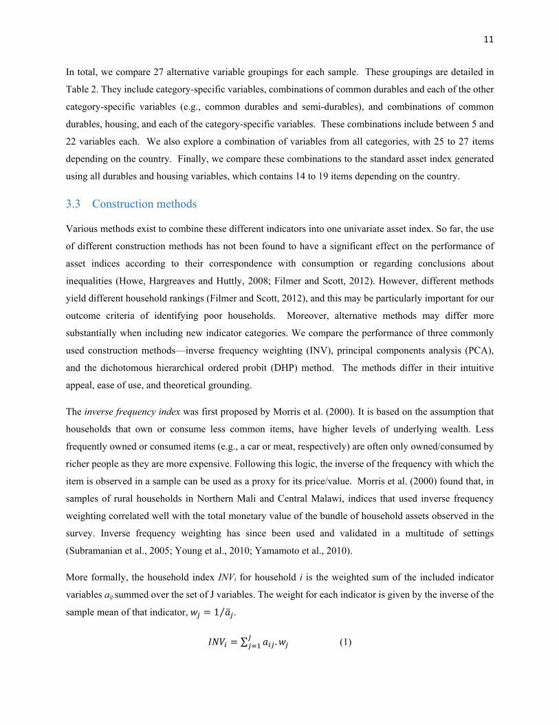
More formally, the household index INVi for household i is the weighted sum of the included indicator

variables aij summed over the set of J variables. The weight for each indicator is given by the inverse of the

sample mean of that indicator, 1⁄ .

∑ . (1)

12  

The inverse frequency method has the advantage of being transparent. It is intuitive and straightforward to

apply.

The second and most widely used construction method is principal components analysis (PCA) (Filmer

and Pritchett, 2001). PCA is a statistical procedure used to reduce multidimensional data into a single

index under the assumption that the included variables can be represented by a set of uncorrelated

components. These components are ordered so that the first component explains the largest amount of

variation in the original data; subsequent components are completely uncorrelated with previous

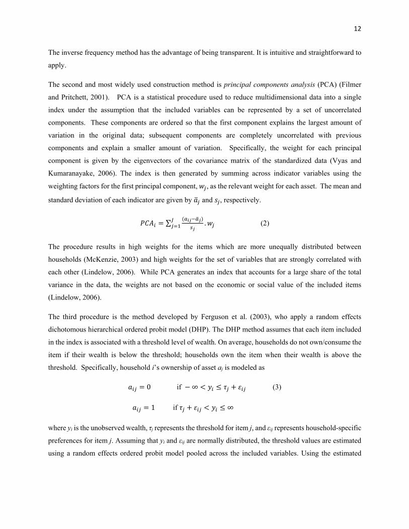
components and explain a smaller amount of variation. Specifically, the weight for each principal

component is given by the eigenvectors of the covariance matrix of the standardized data (Vyas and

Kumaranayake, 2006). The index is then generated by summing across indicator variables using the

weighting factors for the first principal component, , as the relevant weight for each asset. The mean and

standard deviation of each indicator are given by and , respectively.

∑ . (2)

The procedure results in high weights for the items which are more unequally distributed between

households (McKenzie, 2003) and high weights for the set of variables that are strongly correlated with

each other (Lindelow, 2006). While PCA generates an index that accounts for a large share of the total

variance in the data, the weights are not based on the economic or social value of the included items

(Lindelow, 2006).

The third procedure is the method developed by Ferguson et al. (2003), who apply a random effects

dichotomous hierarchical ordered probit model (DHP). The DHP method assumes that each item included

in the index is associated with a threshold level of wealth. On average, households do not own/consume the

item if their wealth is below the threshold; households own the item when their wealth is above the

threshold. Specifically, household i’s ownership of asset aj is modeled as

0if ∞ (3)

1if ∞

where yi is the unobserved wealth, τj represents the threshold for item j, and εij represents household-specific

preferences for item j. Assuming that yi and εij are normally distributed, the threshold values are estimated

using a random effects ordered probit model pooled across the included variables. Using the estimated

13  

thresholds, the index is constructed using the expected value of latent wealth conditional on observed item

ownership following Bayes’ formula.

For example, suppose a household owns only a stove and a bicycle. For each wealth level, the model gives

the conditional probability that the household will own a stove and a bicycle by comparing that wealth level

to the relevant thresholds (Pr | ). The model then computes the probability of having each level of

wealth, conditional on observing ownership of a stove and a bicycle, using the distributional assumptions

over and Bayes’ formula:

Pr |

(4)

This produces a probability distribution for the household’s wealth conditional on its observed bundle.

Finally, the index value is given by | , the expected value of the predicted wealth

distribution for that household.

Ferguson et al. (2003) show that the index performs well in matching income and expenditure using samples

from Greece, Peru, and Pakistan. The method has been used to evaluate program targeting (Lozano et al.,

2006; Gakidou et al., 2007; Lim et al., 2010) and to describe inequalities and risk factors for various health

outcomes (Chatterji et al. 2008; Hall et al. 2009; Patel et al. 2011). Among the three construction methods

applied here, the DHP method provides the most formal connection to economic theory, describing a

specific relationship between underlying wealth and asset ownership. It can be rationalized under

hierarchical preferences but is more computationally intensive than the alternatives (Ngo, 2012).

To date, the three construction methods have been primarily applied to indicators of asset ownership and

housing characteristics. However, they can be readily extended to include dichotomous indicators for semi-

durables and food consumption since the methods are statistical construction methods and mechanically

make no distinction between the types of variables that are included.

3.4 Sample weights

We also vary the samples that are used to calculate the weights when analyzing urban and rural areas. We

test two strategies. The first generates weights (i.e., applies each method) using the entire national sample

and applies these to the urban and rural subsamples; the second generates weights within the urban or rural

subsamples. We do this to assess whether or not the indices are sensitive to different regional patterns of

ownership/consumption since there are some concerns about asset indices being biased against rural areas

(Rutstein and Staveteig, 2014; Wittenberg and Leibbrandt, 2017). We construct all indices separately by

sample. For the urban-specific and rural-specific weights, this allows the meaning of owning a television

14  

in urban Rwanda 2005 to differ from its meaning in rural Rwanda 2005. Using nationally derived weights,

television ownership is assumed to have the same meaning across urban and rural areas within each country-

year.

3.5 Performance criteria

To assess the performance of these different asset indices, we focus on ranking households and identifying

poor households, using consumption as the empirical benchmark, as motivated above. As in most welfare

analysis, we adjust consumption to account for household composition and size. Filmer and Scott (2012)

compare various adult equivalence scales and find that the scaling parameter has little effect on the

correlation between various asset indices and expenditures. We use the Oxford (or OECD) equivalence

scale, which assigns a weight of 1 to the first adult, 0.7 to subsequent adults, and 0.5 to each child, where

children are defined as household members under the age of 15.7

We use three criteria to gauge performance: Spearman rank correlation coefficients, a measure of accuracy

in identifying the extreme poor, and a measure of accuracy in identifying the moderate poor. We use rank

correlation coefficients to assess the correspondence between household rankings derived from the

benchmark and alternative indices. They are affected by correspondence, or lack thereof, across the whole

distribution. To calculate the accuracy measures, poor households are identified as households whose

expenditure is below a given relative poverty line, defining the extreme and moderate poor as the bottom

10 percent and 40 percent of the samples,8 respectively. We use relative poverty lines since the asset indices

generate ordinal rankings.

We define accuracy as the fraction of households correctly classified as poor and non-poor, whereby the

classifications based on per capita expenditures yield the true poor and non-poor groups. This measure

combines both the true positive rate, for those interested in ensuring that poverty programs reach the poor,

and the true negative rate, for those interested in preventing program leakage to non-poor participants.

Formally, this is the Rand accuracy (RA) measure for binary classification (Rand, 1971) applied to poverty

classification:

∑ ∩ ∪ ∩

(5)

                                                            7 http://www.oecd.org/eco/growth/OECD-Note-EquivalenceScales.pdf. 8 The estimated $1.90-day poverty headcount rate for Sub-Saharan Africa is about 40 percent in 2013. The bottom 40 percent also corresponds to the population group tracked under the Shared Prosperity indicator of the World Bank (World Bank, 2015).

15  

1if , 0if

1if , 0if

where captures the relative poverty line (10 percent and 40 percent), and denote whether or

not household i is poor according to its consumption or proxy index, respectively, and and capture

the household's rank within the population.

Because we use relative poverty lines, it is possible to achieve high Rand accuracies by randomly

classifying households as poor and non-poor. To see this, under a 10 percent relative poverty line, one

would expect to correctly classify 82 percent of the sample (10 percent of the consumption poor, who make

up 10 percent of the sample and 90 percent of the consumption non-poor, who make up 90 percent of the

sample). Under a 50 percent relative poverty line, we would expect to correctly classify 50 percent of the

sample.

To adjust for this, we use the adjusted Rand index (ARI) described by Hubert and Arabie (1985) to correct

for chance classification. The ARI is defined as

(6)

capturing the improvement over random classification, normalized by the total possible improvement. The

expected Rand accuracy under random classification, E(RA), is calculated as the sum of the true positive

rate, , and the true negative rate, 1 , associated with random classification.

For example, an index which achieves a raw Rand accuracy of 91 percent under a 10 percent relative

poverty line has a 9 percentage point gain over random classification (E(RA) = 82 percent) out of a possible

18 percentage points, giving it an ARI of 50 percent. If the index improves on random targeting, the ARI

takes on a positive value. If it performs worse, its value is negative.

Within the literature on clustering and classification, the ARI is the preferred measure for comparing two

partitions (Warrens, 2008; Steinly, Brusco, and Hubert, 2016) and has been used extensively in various

fields including psychology (Steinley, Brusco, and Hubert, 2016), bioinformatics (Yeung and Ruzzo, 2001),

and computer science and engineering (Park and Jun, 2009).

3.6 Meta-analysis

Application of these methods and performance comparisons across different settings and periods (13

country-year combinations in five countries at national, urban, and rural levels) further enables us to begin

16  

to analyze whether there are any systematic patterns in the way the different features of the asset index

(variable combination, construction method, sampling weights) affect the performance of these indices.

While all five countries are from Sub-Saharan Africa, they cover a wide array of agro-ecological, socio-

economic, and cultural settings. There are similarities in the included items9 but also notable differences.10

If, despite these differences, asset indices with certain features (e.g., those including food items) perform

systematically better or worse, this would provide important insights to guide the construction and use of

such indices in other settings.

To explore this, we first simply identify the top performing variable combinations in the national, urban,

and rural samples according to our three performance criteria, restricting our analysis to indices constructed

using national weights generated from PCA. This gives a sense of the performance of the different variable

combinations and helps identify those that perform well without making any assumptions about similarities

across samples. Second, to get a more systematic view and identify the difference in performance by

indicator categories, construction methods, and sampling weights, we subsequently pool the samples and

conduct a meta-regression.

Specifically, we perform a separate regression for each of the three criteria (correlation, ARI under a 10

percent poverty line, and ARI under a 40 percent poverty line) and examine how the different factors in

constructing the indices affect the performance. For each criteria, we pool the scores for the 13 national

samples and for all the 81 indices constructed within each sample (27 variable combinations and 3

construction methods). We then regress the performance score on indicators for each variable combination

and construction method, including survey (country-by-year) dummies to capture differences in overall

performance levels across time and space. The meta-regression thus calculates the within-survey

differences between indices and averages these across all surveys, controlling for various dimensions of

how the indices are constructed and allowing for statistical inference using a regression framework. We

cluster standard errors by country. For the national samples, the regression is given by:

(7)

                                                            9 First, as described above, we include many of the same items in the different variable categories. For example, the meat category within foods includes cooking oil, fish, milk, and eggs in all countries. We also restrict our analysis of durables to a similar number of items. Second, there are empirical similarities in the underlying consumption and ownership patterns in all the included countries. For example, the most common staples include maize and the most common durable goods include furniture and radios. 10 First, items differ due to survey design. For example, some surveys list “furniture” as a durable good, while other surveys are more specific in including “beds”, “tables”, or “chairs.” Second, due to economic and cultural differences between the countries and over time, the same items may represent different levels of economic status due to differences in quality, preferences, or relative prices. 

17  

where v indexes variable combinations, m indexes construction methods, c indexes countries, and t indexes

survey waves. Score is the relevant performance criteria (correlation or accuracy measure), Var combo is

a set of dummies for the combinations of included variables, Method is a set of dummies for the construction

method (INV, PCA, or DHP), and Survey is a set of dummies for the country-years.

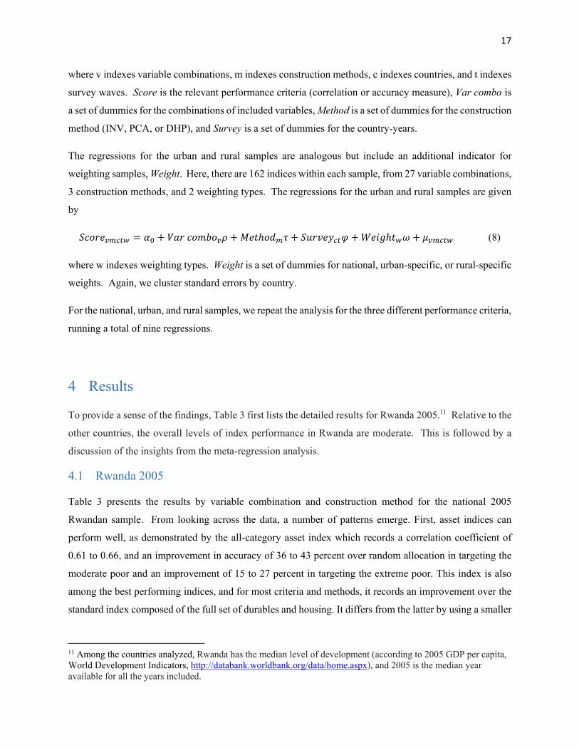
The regressions for the urban and rural samples are analogous but include an additional indicator for

weighting samples, Weight. Here, there are 162 indices within each sample, from 27 variable combinations,

3 construction methods, and 2 weighting types. The regressions for the urban and rural samples are given

by

(8)

where w indexes weighting types. Weight is a set of dummies for national, urban-specific, or rural-specific

weights. Again, we cluster standard errors by country.

For the national, urban, and rural samples, we repeat the analysis for the three different performance criteria,

running a total of nine regressions.

4 Results

To provide a sense of the findings, Table 3 first lists the detailed results for Rwanda 2005.11 Relative to the

other countries, the overall levels of index performance in Rwanda are moderate. This is followed by a

discussion of the insights from the meta-regression analysis.

4.1 Rwanda 2005

Table 3 presents the results by variable combination and construction method for the national 2005

Rwandan sample. From looking across the data, a number of patterns emerge. First, asset indices can

perform well, as demonstrated by the all-category asset index which records a correlation coefficient of

0.61 to 0.66, and an improvement in accuracy of 36 to 43 percent over random allocation in targeting the

moderate poor and an improvement of 15 to 27 percent in targeting the extreme poor. This index is also

among the best performing indices, and for most criteria and methods, it records an improvement over the

standard index composed of the full set of durables and housing. It differs from the latter by using a smaller

                                                            11 Among the countries analyzed, Rwanda has the median level of development (according to 2005 GDP per capita, World Development Indicators, http://databank.worldbank.org/data/home.aspx), and 2005 is the median year available for all the years included.   

18  

set of durables (only the five most common) and adding some indicators of staple, non-staple, and semi-

durable consumption.

Second, there is considerable variation in performance depending on the variable combinations. Indices

with more indicators tend to perform better on average, though adding indicators does not guarantee better

performance. Much depends on the categories of variables included. Single food and housing category

indices (which often have 5-10 indicators) tend to perform worst in this case. Yet, even on their own, and

with a similar number of indicators, the semi-durable and the full durable indicator categories (5 and 12

indicators, respectively), do well, with the exception of identifying the extreme poor using the full durable

list.

Performance of the asset indices improves when combining the short list of durables (the five most common

ones) with any of the other categories (Table 3, common durables and one other category), but especially

when combining the 5 most common durables with semi-durables or housing characteristics (still only 10

items in total). Combining all three (5 most common durables, housing characteristics, and semi-durable

indicators – or 15 indicators) performs almost as well as the standard and all-category asset index. Adding

food categories (all-category asset index) improves the performance in terms of identifying the poor (at

least for the INV and DHP construction methods).

Third, we do not find consistency in which construction method performs best. When taking the Spearman

rank correlation coefficient as the criterion, the PCA construction method tends to do better. Within the

ARI measures, there are sometimes moderate to larger differences between construction methods,

particularly among the ARI for the extreme poor. The INV and DHP methods tend to perform similarly,

while the PCA method differs more noticeably.

Fourth, compared to the national sample, the overall levels of performance across all criteria are higher in

the urban sample (Appendix Table A.1) and lower in the rural sample (Appendix Table A.2).12 The pattern

of performance across the different indicator categories in the urban sample is similar to the national sample

and there is little variation in performance between national and urban weighting for most of the higher

performing variable combinations. In the rural sample, with a correlation coefficient of 0.58 (rural weights),

an ARI for the extreme poor of 0.24 (rural weights), and an ARI for the moderate poor of 0.38 (rural

weights), the top performing variable combination is also the all-category index. A few other indices also

perform better than the standard full asset index (durables, housing), especially when identifying the

extreme poor and using rural instead of national weights. These include the 15-item combination of

                                                            12 Results are only presented for the PCA construction method.

19  

common durables, housing, and semi-durables and the 20-item combination of common durables, housing,

and common foods. Within most variable combinations, the rural weights do better than the national

weights, with larger differentials when examining the ARI for the extreme poor.

Finally, we note that across indices, construction methods and settings, the performance is lowest when

identifying the extreme poor (bottom 10 percent). The fewer poor there are, the harder it becomes to identify

them.13 In addition, since the potential gains in accuracy over random classification are small (18 percentage

points over correctly classifying 82 percent of the population at random), it is difficult to achieve high ARIs

even with relatively high raw accuracies. For example, raw accuracies of 0.85 and 0.90 are associated with

ARIs of 0.15 and 0.44, respectively.

4.2 Meta-analysis

To determine whether the patterns identified in Rwanda 2005 are consistent across settings and periods, we

conduct a meta-analysis. To give a sense of the findings, we first list the two best performing indices

according to the correlation coefficient (Table 4) and the ARI (Table 5), for all countries, including the

national samples from all years and the urban and rural samples from the first wave in each country.

Appendix Tables A.3 and A.4 present the analogous results for the urban and rural samples from the second

and third waves in each country. The all-category index frequently appears among the two highest

performing indices across settings, periods, and performance criterion (correlation and ARI). When looking

at correlations, the combination of common durables, housing, and semi-durables (dur1, house, semi-dur)

also appears frequently among the top two, especially in Uganda, Rwanda, and Ghana, while indices using

food variables on their own or in combination with common assets and housing also perform well in

Malawi, Uganda, and Tanzania. In identifying both the extreme poor and moderate poor, combinations

which include food variables (either staples, non-staples, or both) appear among the highest performers for

many of the samples.

Table 6 presents the results of the full meta-analysis regression described in equations 7 and 8 above. The

results from the meta-analysis are confirmed when doing the meta-analysis country by country.14 While

we include all variable combinations in the regression, we only show the results for the top 10 performing

combinations (as identified by the combinations that occurred most commonly in Table 4, Table 5,

                                                            13 Incidentally, and in the same vein, the World Bank’s target of eradicating extreme poverty is in effect set at bringing the world’s headcount ratio of extreme poor (defined as living on less than $1.90/day (2011 PPP US$) to less than 3 percent, not zero. 14 The results are available from the authors upon request. Performing the meta-analysis country by country allows for greater flexibility in the coefficients across settings. Yet, it largely defeats the purpose of the meta-analysis, given that there are only two or three observations per country, making it hard to detect statistically significant results. Compared to the pooled meta-regression, we find very similar patterns but less statistical significance. 

20  

Appendix Table A.3, and Appendix Table A.4). The full meta-regression results are shown in Appendix

Table A.5. The omitted categories are the standard asset indices (all durables and housing variables) and

the PCA construction method. The omitted survey is Malawi 2004, where Malawi has the lowest 2005 GDP

per capita. In the urban and rural analyses, the omitted weights are urban-specific and rural-specific weights,

respectively. Negative coefficients indicate that the indicator combinations and construction methods

underperform compared to these reference indices while positive coefficients measure potential gains in

using alternative variables, construction methods, and sample weights.

Using the reference index (standard asset index, PCA, national sample weights), overall performance levels

are good, consistent with the first insight from the Rwanda 2005 results. In the national samples,

correlations range from 0.42 (Ghana 1991) to 0.67 (Tanzania 2008), while the ARI values range from 0.25

(Ghana 1991) to 0.44 (Uganda 2005) for identifying the moderate poor and from 0.08 (Rwanda 2000) to

0.31 (Tanzania 2010) for identifying the extreme poor. This can be seen from looking across the coefficients

on the constant and the country-year indicator variables (Appendix Table A.5). The indices perform

generally worse in Ghana, the country with the highest 2005 GDP per capita. When using the reference

index, performance is usually also better in the urban samples and worse in the rural samples, compared

with the national sample. This holds across countries. Finally, identifying the extreme poor proves the most

challenging, making methods which improve performance there particularly attractive.

Turning to the performance of the different indicator combinations, the standard asset index (about 17

indicators consisting of all durables and housing characteristics with PCA) performs best in the urban

sample (or at least as well as the all-category index and the common durable, housing, and semi-durable

index). This holds across performance criteria and construction methods. This can be seen from the many

negative signs on the coefficients across the different indices, which are often also statistically significant.

Where the coefficient is positive (such as for the all-category index for the extreme poor), it is small and

not statistically significant. These results provide support for the use of the standard asset index in urban

settings to rank households and identify the poor. Deriving the weights from the national sample, instead

of from the urban sample, can further improve the performance.

Yet, meaningful improvements in performance can be obtained in other settings. In the national sample,

this holds for identifying the extreme poor. There, targeting performance can be improved by an estimated

11 percentage points by using the all-category index. Targeting of the extreme poor can also be improved

using other indices with 15 to 20 variables, such as those using common durables, housing characteristics,

and either common staples or non-staples (an estimated improvement in targeting accuracy of 4 percentage

points) or common foods (an estimated improvement in targeting accuracy of 6 percentage points). Using

21  

different indices did not lead to statistically significant improvements in the national sample for the other

performance criteria or when using other construction methods (INV or DHP).

In rural settings, the all-category index outperforms the standard index for all performance criteria, by an

estimated 9 points for ranking households, and by 12 percentage points and 8 percentage points for

identifying the extreme and moderate poor, respectively (all statistically significant at the 1 percent level

or higher). When it comes to identifying the extreme poor, other combinations of common durables,

housing characteristics, and one other category (common staples, non-staples, or common foods) also

outperform the standard index. There are no significant differences comparing across construction methods

or when comparing national weights to rural weights.

5 Concluding Remarks

Collecting data to rank households and target the poorer segments of society is costly. Statistical asset

indices, especially those using information on ownership of common durables and housing characteristics

and constructed using principal components analysis, have been frequently used as alternatives to

consumption measures. However, rankings have been found to differ compared with those obtained using

consumption, which is still considered the benchmark. Moreover, asset indices often have difficulty

distinguishing among the poorest households, particularly in rural areas, since many do not own any of the

included durables and housing variables.

This paper systematically examines whether the performance of the standard asset indices can be improved

upon by using dichotomous indicators of staple food, non-staple food, and semi-durable consumption,

either on their own, or in combination with common durables. It does so by examining their performance

in ranking households across the whole distribution and identifying extreme and moderately poor

populations using 13 different survey waves in national, rural, and urban settings from five African

countries.

The following insights emerge. First, the use of asset indices constructed from dichotomous variables from

a range of categories holds promise, often generating rank correlation coefficients in the 0.60 to 0.70 range

and accuracy improvements on the order of 30 to 40 percent. This is consistent with previous literature

validating proxies for consumption using a variety of performance criteria. This suggests that these methods

can be used to rank households and target poverty programs in a range of contexts, including in urban and

rural subsamples.

22  

Second, the findings indicate that the standard asset indices combining durables and housing variables

perform well. They perform at least as well and generally better than other variable combinations in urban

samples when ranking households and identifying both the extreme and moderate poor and in national

samples when ranking households and identifying the moderate poor. This suggests that durables and

housing variables display good discriminatory power among households with slightly higher incomes.

Third, performance can be improved upon, however, in rural settings and in identifying the extreme poor

in national settings by complementing the standard asset index with information on staple and non-staple

foods and semi-durables. Such an all-category index yields an average improvement over the standard asset

index of 9 points in the Spearman rank correlation across all households, and of 12 and 8 percentage points

in identifying the extreme and moderate poor, respectively. These are meaningful improvements that come

at little extra cost, especially in the African context where four in five of Africa’s poor are still concentrated

in rural areas (Beegle et al., 2016).

Fourth, decisions regarding construction and construction methods appear less important. Indices generated

using PCA perform slightly better than the two other construction methods, but the differences are small

and not always statistically significant. Similarly, weights can be generated from within a sample or from

a larger representative sample without substantially altering index performance (except in the urban

sample).

Overall, the results suggest that policy makers and researchers who are interested in inexpensively

identifying poor households should consider adding information on consumption to the information base

included in standard asset indices. This is particularly relevant for those interested in identifying the

extreme poor, and particularly in rural settings. Specifically, survey instruments can be designed to include

yes/no indicators for a short list of variables from the categories of durable ownership, housing

characteristics, staple food consumption, non-staple food consumption, and semi-durable consumption.

The results suggest that including five commonly owned/consumed items within each category provides

reasonable power to differentiate between households.

This modification could be implemented at reasonably low cost, since it requires information on a very

small number of additional items and only on whether these have been consumed or not (not how much).

Because a large share of the data collection cost consists of visiting the household (transport and search

costs), the marginal cost to asking a few additional questions once there is very low. For a more detailed

discussion of the trade-offs between gains in precision and data collection costs, see for example Fujii and

van der Weide (2016).

23  

Moreover, the proposed data collection efforts are feasible, since new data are abundant and new survey

instruments are being contextualized to meet the goals of each study. For example, recently developed

methods such as the Simple Poverty Scorecard and the Survey of Well-Being via Instant and Frequent

Tracking are used by microfinance institutions, NGOs, and businesses, and there is increased interest in

low-cost randomized-controlled trials using shorter data collection instruments. Even more standardized,

cross-country survey series continue to change constantly. For example, in the DHS instruments, there has

been an increase in the number of durable ownership items included over time since the use of asset indices

has become commonplace. In addition, new topic-specific modules are introduced and changed regularly,

and countries often add context-specific questionnaires and items to match with their needs. These many

efforts to collect better data are in line with the movement toward more frequent and more meaningful data

collection efforts to promote evidence-based sustainable development (Millennium Development Goals

Report, 2015).

In conclusion, this work adds to our understanding of the performance of asset indices and their ability to

proxy for consumption, and it provides policy-relevant insights for ongoing data collection efforts.

Additional research is necessary on the properties of asset indices, such as their performance in capturing

changes in consumption over time, in a wider range of settings, across a broader range of poverty cut-offs,

and using multiple performance criteria. With this ongoing research, the profession can further help refine

practitioner guidelines on how to collect and combine inexpensive and reliable data to improve poverty

analyses in developing countries.

24  

6 References

Acham, H., Kikafunda, J., Malde, M., Oldewage-Theron, W., & Egal, A. (2012). Breakfast, midday meals and academic achievement in rural primary schools in Uganda: implications for education and school health policy. Food & Nutrition Research, 56, 1-12.

Alkire, S., & Santos, M. E. (2014). Measuring acute poverty in the developing world: Robustness and scope of the multidimensional poverty index. World Development, 59, 251-274.

Bader, C., Bieri, S., Wiesmann, U., & Heinimann, A. (2017). Is economic growth increasing disparities? A multidimensional analysis of poverty in the Lao PDR between 2003 and 2013. The Journal of Development Studies, 53(12), 2067-2085.

Baker, F., & Kim, S. (2004). Item Response Theory: Parameter Estimation Techniques (2nd ed.). New York: Marcel Dekker Inc.

Beegle, K., Christiaensen, L., Dabalen, A., & Gaddis, I. (2016). Poverty in a Rising Africa. Washington, D.C.: World Bank.

Caldas, M., Walker, R., Arima, E., Perz, S., Aldrich, S., & Simmons, C. (2007). Theorizing Land Cover and Land Use Change: The Peasant Economy of Amazonian Deforestation. Annuals of the Association of American Geographers, 97(1), 86-110.

Chatterji, S., Kowal, P., Mathers, C., Naidoo, N., Verdes, E., Smith, J. P., & Suzman, R. (2008). The health of aging populations in China and India. Health Affairs, 27(4), 1052-1063.

Christiaensen, L., Lanjouw, P., Luoto, J., & Stifel, D. (2012). Small area estimation-based prediction methods to track poverty: validation and applications. Journal of Economic Inequality, 10(2), 267-297.

Coady, D., Grosh, M., & Hoddinott, J. (2004). Targeting outcomes redux. The World Bank Research Observer, 19(1), 61-85.

Deaton, A. (2006). Measuring Poverty. In A. V. Banerjee, R. Benabou, & D. Mookherjee, Understanding Poverty. Oxford: Oxford University Press.

Deaton, A., & Zaidi, S. (2002). Guidlines for construction consumption aggregates for welfare analysis. World Bank Publications, 135.

Diamond, A., Gill, M., Rebolledo Dellepiane, M. A., Skoufias, E., Vinha, K., & Xu, Y. (2016). Estimating poverty rates in target populations: An assessment of the simple poverty scorecard and alternative approaches. Washington, D.C.: World Bank.

Douidich, M., Ezzrari, A., Van der Weide, R., & Verme, P. (2016). Estimating quarterly poverty rates using labor force surveys: a primer. The World Bank Economic Review, 30(3), 475-500.

Ferguson, B., Tandon, A., Gakidou, E., & Murray, C. (2003). Estimating Permanent Income Using Indicator Variables. World Health Organization.

25  

Ferreira, F. H., & Lugo, M. A. (2013). Multidimensional poverty analysis: Looking for a middle ground. The World Bank Research Observer , 28(2), 220-235.

Filmer, D., & Pritchett, L. (2001). Estimating wealth effects without expenditure data-or tears: an application to education al enrollments in states of India. Demography, 38(1), 115-132.

Filmer, D., & Scott, K. (2012). Assessing Asset Indices. Demography, 49, 359-392.

Friedman, M. (1957). A theory of the consumption function. Princeton, New Jersey: Princeton University Press.

Fujii, T., & van der Weide, R. (2016). Is Predicted Data a Viable Alternative to Real Data? World Bank Policy Research Working Paper, 7841.

Gakidou, E., Oza, S., Fuertes, C. V., Li, A. Y., Lee, D. K., Sousa, A., Hogan, M. C., Vander Hoorn, S., & Ezzati, M. (2007). Improving child survival through environmental and nutritional interventions: the importance of targeting interventions toward the poor. Journal of American Medical Association, 298(16), 1876-1887.

Gunning, J., Hoddinott, J., Kinsey, B., & Owens, T. (2000). Revisiting forever gained: Income dynamics in the resettlement areas of Zimbabwe, 1983-96. Journal of Development Studies, 36(6), 131-154.

Gwatkin, D. R., Rutstein, S., Johnson, K., Suliman, E., Wagstaff, A., & Amouzou, A. (2007). Socio-economic differences in health, nutrition, and population within developing countries. Washington, D.C.: The World Bank.

Gwatkin, D. R., Wagstaff, A., & Yazbeck, A. S. (2005). What did the reaching the poor studies find? In D. R. Gwatkin, A. Wagstaff, & A. S. Yazbeck, Reaching the Poor with Health, Nutrition and Population Services (p. 47). The World Bank.

Hall, J. N., Moore, S., Harper, S. B., & Lynch, J. W. (2009). Global variability in fruit and vegetable consumption. American Journal of Preventive Medicine, 36(5), 402-409.

Handa, S., & Davis, B. (2006). The experience of conditional cash transfers in Latin America and the Caribbean. Development policy review, 24(5), 513-536.

Harttgen, K., Klasen, S., & Vollmer, S. (2013). An African growth miracle? Or: what do asset indices tell us about trends in economic performance? Review of Income and Wealth, 59.S1.

Holmes, C. (2003). Assessing the perceived utility of wood resources in a protected area of Western Tanzania. Biological Conservation, 111, 179-189.

Houweling, T., Kunst, A., & Mackenbach, J. (2003). Measuring health inequality among children in developing countries: does the choice of indicator of economic status matter? International Journal for Equity in Health, 2(8), 8-19.

Howe, L., Hargreaves, J., & Huttly, S. (2008). Issues in the construction of wealth indices for measurement of socio-economic position in low-income countries. Emerging Themes in Epidemiology, 5(3).

26  

Howe, L., Hargreaves, J., Gabrysch, S., & Huttly, S. (2009). Is the wealth index a proxy for consumption expenditure? A systematic review. Journal of Epidemiology and Community Health, 63, 871-880.

Hubert, L., & Arabie, P. (1985). Comparing partitions. Journal of classification, 2(1), 193-218.

Lim, S. S., Dandona, L., Hoisington, J. A., James, S. L., Hogan, M. C., & Gakidou, E. (2010). India's Janani Suraksha Yojana, a conditional cash transfer programme to increase births in health facilities: an impact evaluation. The Lancet, 375(9730), 2009-2023.

Lindelow, M. (2006). Sometimes more equal than others: how health inequalities depend on the choice of welfare indicator. Health Economics, 15(3), 263-279.

Lozano, R., Soliz, P., Gakidou, E., Abbott-Klafter, J., Feehan, D. M., Vidal, C., Ortiz, J. P., & Murray, C. J. L. (2006). Benchmarking of performance of Mexican states with effective coverage. The Lancet, 369(9548), 1729-1741.

Maitra, S. (2016). The poor get poorer: Tracking relative poverty in India using a durables-based mixture model. Journal of Development Economics, 110-120.

McKenzie, D. (2003). Measure inequality with asset indicators. Cambridge, MA: Center for International Development, Harvard University.

Meyer, B. D., & Sullivan, J. X. (2003). Measuring the Well-Being of the Poor Using Income and Consumption. Journal of Human Resources, 1180-1220.

Montgomery, M., & Hewett, P. (2005). Urban poverty and health in development countries: household and neighborhood effects. Demography, 42(3), 397-425.

Morris, S., Carletto, C., Hoddinott, J., & Christiaensen, L. (2000). Validity of rapid estimates of household wealth and income for health surveys in rural Africa. Journal of Epidemiology and Community Health, 54, 381-387.

Ngo, D. (2018). A theory-based living standards index for measuring poverty in developing countries. Journal of Development Economics, 130, 190-202.

Ngo, D. K. (2012). TVs, Toilets, and Thresholds: Measuring Wealth Comparably Using and Asset-Based Index. Northeast Universities Development Consortium Conference. Hanover, NH. Retrieved from http://www.dartmouth.edu/~neudc2012/docs/paper_193.pdf

Park, H.-S., & Jun, C.-H. (2009). A simple and fast algorithm for K-medoids clustering. Expert systems with applications, 36(2), 3336-3341.

Patel, V., Chatterji, S., Chisholm, D., Ebrahim, S., Gopalakrishna, G., Mathers, C., Mohan, V., Prabhakaran, D., Ravindran, R. D., & Reddy, K. S. (2011). Chronic diseases and injuries in India. The Lancet, 377(9763), 413-428.

Perry, B. (2002). The mismatch between income measures and direct outcome measures of poverty. Social Policy Journal of New Zealand, 19, 101-27.

27  

Poterba, J. M. (1991). Is the Gasoline Tax Regressive? Tax Policy and the Economy, 5, 145-164.

Rand, W. M. (1971). Objective criteria for the evaluation of clustering methods. Journal of the American Statistical Association, 66(336), 846-850.

Ravallion, M. (2015). The economics of poverty: History, measurement, and policy. Oxford: Oxford University Press.

Rutstein, S. O., & Johnson, K. (2004). The DHS wealth index. DHS comparative reports. No. 6. Calverton: ORC Macro.

Rutstein, S. O., & Staveteig, S. (2014). Making the Demographic and Health Surveys wealth index comparable. ICF International.

Sahn, D. E., & Stifel, D. (2003). Exploring alternative measures of welfare in the absence of expenditure data. Review of income and wealth, 49(4), 463-489.

Sahn, D. E., & Stifel, D. C. (2000). Poverty comparisons over time and across countries in Africa. World development, 28(12), 2123-2155.

Simmons, C., Walker, R., Perz, S., Aldrich, S., Caldas, M., Pereira, R., Leite, F, Fernandes, L. C., & Arima, E. (2009). Doing if for Themselves: Direct Action Land Reform in the Brazilian Amazon. World Development, 38(3), 429-444.

Steinley, D., Brusco, M. J., & Hubert, L. (2016). The variance of the adjusted Rand index. Psychological Methods, 21(2), 261.

Stifel, D., & Christiaensen, L. (2007). Tracking Poverty Over Time in the Absence of Comparable Consumption Data. The World Bank Economic Review, 21(2), 317-341.

Subramanian, S., Nandy, S., Irving, M., Gordon, D., & Smith, G. D. (2005). Role of socioeconomic markers and state prohibition policy in predicting alcohol consumption among men and women in India: a multilevel statistical analysis. Bulletin of the World Health Organization, 83, 829-836.

United Nations. (2015). The Millennium Development Goals Report. Washington, DC: United Nations.

Vyas, S., & Kumaranayake, L. (2006). Constructing socio-economic status indices: how to use principal components analysis. Health Policy and Planning, 21(6), 459-68.

Wagstaff, A., & Watanabe, N. (2003). What difference does the choice of SES make in health inequality measurement? Health Economics, 12, 885-890.

Warrens, M. J. (2008). On the equivalence of Cohen’s kappa and the Hubert-Arabie adjusted Rand index. Journal of Classification, 25(2), 177-183.

Wittenberg, M., & Leibbrandt, M. (2017). Measuring Inequality by Asset Indices: A General Approach with Application to South Africa. Review of Income and Wealth, 63(4), 706-730.

28  

World Bank. (2000). World Development Report 2000-2001: Attacking Poverty. Washington, DC: World Bank Group.

World Bank. (2015). A Measured Approach to Ending Poverty and Boosting Shared Prosperity - Concepts, Data and the Twin Goals. Washington, D.C.: World Bank.

Yamamoto, S., Louis, V., Sie, A., & Sauerborn, R. (2010). Household risk factors for clinical malaria in a semi-urban area of Burkina Faso: a case-control study. Transactions of the Royal Society of Tropical Medicine and Hygiene, 104(1), 61-65.

Yeung, K. Y., & Ruzzo, W. L. (2001). Principal component analysis for clustering gene expression data. Bioinformatics, 17(9), 763-774.

Young, A. (2012). The African Growth Miracle. Journal of Political Economy, 120(4), 696-739.

Young, S. L., Khalfan, S. S., Farag, T. H., Kavle, J. A., Ali, S. M., Hajji, H., Rasmussen, K. M., Pelto, G. H., Tielsch, J. M., & Stoltzfus, R. J. (2010). Association of pica with anemia and gastrointestinal distress among pregnant women in Zanzibar, Tanzania. The American Journal of Tropical Medicine and Hygiene, 83(1), 144-151.

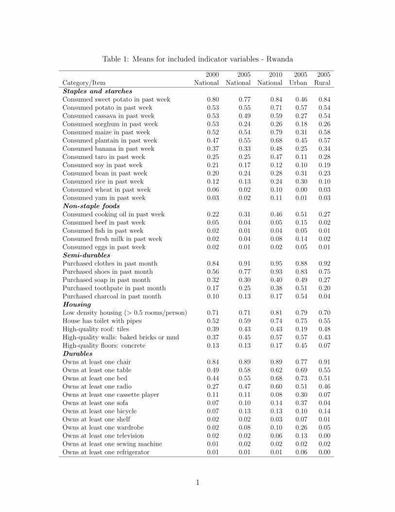
Table 1: Means for included indicator variables - Rwanda

2000 2005 2010 2005 2005Category/Item National National National Urban RuralStaples and starchesConsumed sweet potato in past week 0.80 0.77 0.84 0.46 0.84Consumed potato in past week 0.53 0.55 0.71 0.57 0.54Consumed cassava in past week 0.53 0.49 0.59 0.27 0.54Consumed sorghum in past week 0.53 0.24 0.26 0.18 0.26Consumed maize in past week 0.52 0.54 0.79 0.31 0.58Consumed plantain in past week 0.47 0.55 0.68 0.45 0.57Consumed banana in past week 0.37 0.33 0.48 0.25 0.34Consumed taro in past week 0.25 0.25 0.47 0.11 0.28Consumed soy in past week 0.21 0.17 0.12 0.10 0.19Consumed bean in past week 0.20 0.24 0.28 0.31 0.23Consumed rice in past week 0.12 0.13 0.24 0.30 0.10Consumed wheat in past week 0.06 0.02 0.10 0.00 0.03Consumed yam in past week 0.03 0.02 0.11 0.01 0.03Non-staple foodsConsumed cooking oil in past week 0.22 0.31 0.46 0.51 0.27Consumed beef in past week 0.05 0.04 0.05 0.15 0.02Consumed fish in past week 0.02 0.01 0.04 0.05 0.01Consumed fresh milk in past week 0.02 0.04 0.08 0.14 0.02Consumed eggs in past week 0.02 0.01 0.02 0.05 0.01Semi-durablesPurchased clothes in past month 0.84 0.91 0.95 0.88 0.92Purchased shoes in past month 0.56 0.77 0.93 0.83 0.75Purchased soap in past month 0.32 0.30 0.40 0.49 0.27Purchased toothpate in past month 0.17 0.25 0.38 0.51 0.20Purchased charcoal in past month 0.10 0.13 0.17 0.54 0.04HousingLow density housing (> 0.5 rooms/person) 0.71 0.71 0.81 0.79 0.70House has toilet with pipes 0.52 0.59 0.74 0.75 0.55High-quality roof: tiles 0.39 0.43 0.43 0.19 0.48High-quality walls: baked bricks or mud 0.37 0.45 0.57 0.57 0.43High-quality floors: concrete 0.13 0.13 0.17 0.45 0.07DurablesOwns at least one chair 0.84 0.89 0.89 0.77 0.91Owns at least one table 0.49 0.58 0.62 0.69 0.55Owns at least one bed 0.44 0.55 0.68 0.73 0.51Owns at least one radio 0.27 0.47 0.60 0.51 0.46Owns at least one cassette player 0.11 0.11 0.08 0.30 0.07Owns at least one sofa 0.07 0.10 0.14 0.37 0.04Owns at least one bicycle 0.07 0.13 0.13 0.10 0.14Owns at least one shelf 0.02 0.02 0.03 0.07 0.01Owns at least one wardrobe 0.02 0.08 0.10 0.26 0.05Owns at least one television 0.02 0.02 0.06 0.13 0.00Owns at least one sewing machine 0.01 0.02 0.02 0.02 0.02Owns at least one refrigerator 0.01 0.01 0.01 0.06 0.00

1

Table 2: Variable combinations (Rwandan sample)

# ofVariable group items Included variables

Single categories and short listsStaples and other starches, full 13 Plantain, sweet potato, cassava, sorghum, wheat, yam,

potato, taro, soy, banana, maize, rice, beanStaples, list 1, most common 5 Sweet potato, potato, cassava, sorghum, maizeStaples, list 2, low correlation 5 Bean, cassava, rice, sorghum, wheatNon-staple foods 5 Beef, fish, fresh milk, egg, cooking oilFoods, full 18 Full list of staples and non-staplesFoods, list 1, most common 10 Non-staples and five most common staplesFoods, list 2, low correlation 10 Non-staples and five low correlation staplesSemi-durables 5 Clothes, shoes, toothpaste, soap, charcoalHousing 5 Quality roof, low density housing, toilet, quality floor,

quality wallsDurables, full 12 Sofa, fridge, radio, cassette player, television, sewing

machine, bed, wardrobe, shelf, table, chair, bikeDurables, list 1, most common 5 Chair, table, bed, radio, cassette playerDurables, list 2, low correlation 5 Bike, chair, radio, sewing machine, television

Common durables and one other categoryDurables 1 and staples 1 10 Five most common durables, five most common staplesDurables 1 and staples 2 10 Five most common durables, five low correlation staplesDurables 1 and non-staples 10 Five most common durables, non-staplesDurables 1 and food 1 15 Five most common durables, five most common staples,

non-staplesDurables 1 and food 2 15 Five most common durables, five low correlation staples,

non-staplesDurables 1 and semi-durables 10 Five most common durables, semi-durablesDurables 1 and housing 10 Five most common durables, housing

Common durables, housing, and one other categoryDurables 1, housing, staples 1 15 Five most common durables, housing, five most common

staplesDurables 1, housing, staples 2 15 Five most common durables, housing, five low correla-

tion staplesDurables 1, housing, non-staples 15 Five most common durables, housing, non-staplesDurables 1, housing, food 1 20 Five most common durables, housing, five most common

staples, non-staplesDurables 1, housing, food 2 20 Five most common durables, housing, five low correla-

tion staples, non-staplesDurables 1, housing, semi-durables 15 Five most common durables, housing, semi-durables

All-category indexDur1, house, food1, semi-durables 25 Five most common durables, housing, five most common

staples, non-staples, semi-durables

Standard asset indexDurables and housing 17 All durables, housing

2

Table 3: Index performance by construction method and variable combination, Rwanda2005, national sample

Spearman Adj. Rand index, Adj. Rand index,rank correlation extreme poor moderate poor

No. coefficient (bottom 10% ) (bottom 40% )

of Method Method MethodIndex var. INV PCA DHP INV PCA DHP INV PCA DHP

Single categories and short listsStaples, full 13 0.13 -0.05 0.09 0.11 -0.08 0.11 0.16 0.05 0.14Staples 1 5 -0.05 -0.09 -0.07 -0.04 -0.07 -0.07 0.06 0.04 0.08Staples 2 5 0.15 0.18 0.14 -0.13 -0.67 -0.13 0.09 0.00 0.08Non-staples 5 0.37 0.37 0.37 -2.63 -2.63 -2.63 0.06 0.06 0.06Foods, full 18 0.32 -0.20 0.23 0.18 -0.08 0.17 0.22 0.02 0.21Foods 1 10 0.29 0.28 0.19 0.12 -0.25 0.06 0.21 -0.03 0.17Foods 2 10 0.31 0.35 0.30 0.06 -0.45 0.06 0.11 0.09 0.16Semi-durables 5 0.59 0.60 0.59 0.15 0.15 0.15 0.23 0.23 0.22Housing 5 0.38 0.49 0.39 -0.53 0.11 0.00 0.14 0.25 0.14Durables, full 12 0.58 0.58 0.55 -0.69 -0.41 -0.69 0.34 0.32 0.34Durables 1 5 0.51 0.49 0.45 -0.71 -0.71 -0.75 0.33 0.32 0.31Durables 2 5 0.37 0.23 0.30 0.00 0.00 0.00 0.12 0.12 0.10Common durables and one other categoryDur1, staples1 10 0.40 0.39 0.27 0.19 0.05 0.16 0.33 0.23 0.28Dur1, staples2 10 0.42 0.53 0.41 0.08 0.08 0.08 0.28 0.33 0.29Dur1, non-staples 10 0.57 0.58 0.54 -0.47 -0.47 -0.47 0.36 0.34 0.36Dur1, food1 15 0.51 0.54 0.40 0.22 0.05 0.17 0.36 0.26 0.33Dur1, food2 15 0.48 0.58 0.49 0.16 -0.01 0.16 0.30 0.32 0.32Dur1, semi-durables 10 0.64 0.64 0.61 0.18 0.18 0.18 0.39 0.38 0.38Dur1, house 10 0.54 0.60 0.50 0.07 0.21 0.04 0.34 0.36 0.36Common durables, housing, and one other categoryDur1, house, staples1 15 0.52 0.58 0.40 0.25 0.07 0.22 0.36 0.29 0.35Dur1, house, staples2 15 0.50 0.62 0.49 0.19 0.14 0.21 0.31 0.34 0.35Dur1, house, non-staples 15 0.59 0.64 0.56 0.15 0.20 0.13 0.38 0.36 0.37Dur1, house, food1 20 0.58 0.61 0.49 0.26 0.08 0.25 0.40 0.29 0.38Dur1, house, food2 20 0.54 0.64 0.54 0.19 0.14 0.21 0.32 0.35 0.36Dur1, house, semi-durables 15 0.64 0.67 0.62 0.24 0.22 0.21 0.39 0.40 0.40All-category indexDur1, house, food1, 25 0.66 0.66 0.61 0.27 0.15 0.27 0.43 0.36 0.43semi-durablesStandard asset indexDurables, housing 17 0.58 0.62 0.56 0.08 0.22 0.06 0.35 0.37 0.36

Note: INV refers to the inverse frequency index, PCA refers to the principal components analysis index, and DHPrefers to the dichotomous hierarchical ordered probit index. The number 1 denotes a subset of five common variables,while the number 2 denotes a subset of five low correlation variables.

3

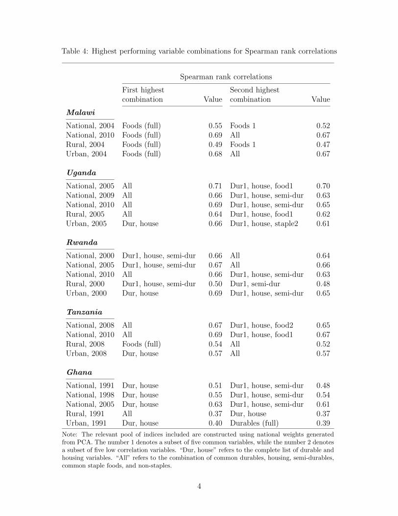
Table 4: Highest performing variable combinations for Spearman rank correlations

Spearman rank correlations

First highest Second highestcombination Value combination Value

Malawi

National, 2004 Foods (full) 0.55 Foods 1 0.52National, 2010 Foods (full) 0.69 All 0.67Rural, 2004 Foods (full) 0.49 Foods 1 0.47Urban, 2004 Foods (full) 0.68 All 0.67

Uganda

National, 2005 All 0.71 Dur1, house, food1 0.70National, 2009 All 0.66 Dur1, house, semi-dur 0.63National, 2010 All 0.69 Dur1, house, semi-dur 0.65Rural, 2005 All 0.64 Dur1, house, food1 0.62Urban, 2005 Dur, house 0.66 Dur1, house, staple2 0.61

Rwanda

National, 2000 Dur1, house, semi-dur 0.66 All 0.64National, 2005 Dur1, house, semi-dur 0.67 All 0.66National, 2010 All 0.66 Dur1, house, semi-dur 0.63Rural, 2000 Dur1, house, semi-dur 0.50 Dur1, semi-dur 0.48Urban, 2000 Dur, house 0.69 Dur1, house, semi-dur 0.65

Tanzania

National, 2008 All 0.67 Dur1, house, food2 0.65National, 2010 All 0.69 Dur1, house, food1 0.67Rural, 2008 Foods (full) 0.54 All 0.52Urban, 2008 Dur, house 0.57 All 0.57

Ghana

National, 1991 Dur, house 0.51 Dur1, house, semi-dur 0.48National, 1998 Dur, house 0.55 Dur1, house, semi-dur 0.54National, 2005 Dur, house 0.63 Dur1, house, semi-dur 0.61Rural, 1991 All 0.37 Dur, house 0.37Urban, 1991 Dur, house 0.40 Durables (full) 0.39

Note: The relevant pool of indices included are constructed using national weights generatedfrom PCA. The number 1 denotes a subset of five common variables, while the number 2 denotesa subset of five low correlation variables. “Dur, house” refers to the complete list of durable andhousing variables. “All” refers to the combination of common durables, housing, semi-durables,common staple foods, and non-staples.

4

Tab

le5:

Hig

hes

tp

erfo

rmin

gva

riab

leco

mbin

atio

ns

for

adju

sted

Ran

din

dex

Adju

sted

Ran

din

dex

,ex

trem

ep

oor

(bot

tom

10%

)A

dju

sted

Ran

din

dex

,m

oder

ate

poor

(bot

tom

40%

)

Fir

sthig

hes

tSec

ond

hig

hes

tF

irst

hig

hes

tSec

ond

hig

hes

tco

mbin

atio

nV

alue

com

bin

atio

nV

alue

com

bin

atio

nV

alue

com

bin

atio

nV

alue

Malawi

Nat

ional

,20

04D

ur1

,fo

od1

0.20

All

0.20

Foods

(full)

0.38

Foods

10.

37N

atio

nal

,20

10A

ll0.

31F

oods

(full)

0.30

Foods

(full)

0.49

All

0.48

Rura

l,20

04D

ur1

,fo

od1

0.17

All

0.16

Foods

(full)

0.34

Foods

10.

33U

rban

,20

04F

oods

(full)

0.37

All

0.36

All

0.48

Foods

(full)

0.46

Uganda

Nat

ional

,20

05A

ll0.

35D

ur1

,hou

se,

food2

0.32

All

0.54

Dur1

,hou

se,

food1

0.52

Nat

ional

,20

09A

ll0.

30D

ur1

,se

mi-

dur

0.28

All

0.41

Dur1

,hou

se,

sem

i-dur

0.38

Nat

ional

,20

10A

ll0.

29D

ur1

,se

mi-

dur

0.29

All

0.48

Dur1

,hou

se,

sem

i-dur

0.45

Rura

l,20

05A

ll0.

32D

ur1

,hou

se,

food2

0.29

All

0.44

Dur1

,hou

se,

food1

0.43

Urb

an,

2005

Dur,

hou

se0.

41D

ur1

,hou

se,

food1

0.39

Dur,

hou

se0.

43D

ur1

,hou

se0.

38

Rwanda

Nat

ional

,20

00D

ur1

,hou

se,

sem

i-dur

0.22

Dur,

hou

se0.

22D

ur1

,hou

se,

sem

i-dur

0.40

Dur1

,se

mi-

dur

0.38

Nat

ional

,20

05D

ur1

,hou

se,

sem

i-dur

0.29

Dur1

,se

mi-

dur

0.28

Dur1

,hou

se,

sem

i-dur

0.41

All

0.40

Nat

ional

,20

10A

ll0.

26D

ur1

,hou

se,

sem

i-dur

0.24

All

0.42

Dur1

,hou

se,

sem

i-dur

0.40

Rura

l,20

00D

ur1

,hou

se,

sem

i-dur

0.22

Dur,

hou

se0.

17D

ur1

,hou

se,

sem

i-dur

0.34

Dur1

,se

mi-

dur

0.33

Urb

an,

2000

All

0.43

Sem

i-dura

ble

s0.

39D

ur,

hou

se0.

51D

ura

ble

s(f

ull)

0.48

Tanza

nia

Nat

ional

,20

08D

ur1

,fo

od1

0.28

All

0.28

All

0.44

Foods

(full)

0.44

Nat

ional

,20

10A

ll0.

34D

ur1

,hou

se,

food1

0.33

All

0.47

Dur1

,hou

se,

food1

0.46

Rura

l,20

08D

ur1

,fo

od1

0.30

Dur1

,hou

se,

food1

0.27

Foods

(full)

0.37

Dur1

,fo

od1

0.33

Urb

an,

2008

Dur1

,hou

se,

food1

0.43

All

0.43

All

0.44

Foods

10.

43

Ghana

Nat

ional

,19

91A

ll0.

33D

ur1

,hou

se,

stap

le1

0.32

Dur,

hou

se0.

34D

ur1

,hou

se,

non

-sta

ple

s0.

32N

atio

nal

,19

98D

ur1

,hou

se,

food1

0.45

All

0.45

All

0.40

Dur1

,hou

se,

stap

le2

0.39

Nat

ional

,20

05A

ll0.

42D

ur1

,hou

se,

food2

0.41

Dur,

hou

se0.

40D

ur1

,hou

se,

sem

i-dur

0.40

Rura

l,19

91D

ur1

,hou

se,

food2

0.30

All

0.30

Dur1

,hou

se,

sem

i-dur

0.26

Dur1

,hou

se,

non

-sta

ple

s0.

26U

rban

,19

91D

ur1

,hou

se,

sem

i-dur

0.25

Dur1

,hou

se,

non

-sta

ple

s0.

25D

ur,

hou

se0.

28D

ura

ble

s(f

ull)

0.28

Note

:T

he

rele

vant

pool

of

indic

esin

cluded

are

const

ruct

edusi

ng

nat

ional

wei

ghts

gen

erate

dfr

om

PC

A.

The

num

ber

1den

otes

asu

bse

tof

five

com

mon

vari

able

s,w

hile

the

num

ber

2den

otes

asu

bse

tof

five

low

corr

elati

onva

riable

s.“D

ur,

house

”re

fers

toth

eco

mple

telist

of

dura

ble

and

housi

ng

vari

able

s.“A

ll”

refe

rsto

the

com

bin

ati

onof

com

mon

dura

ble

s,housi

ng,

Sem

i-dura

ble

s,co

mm

on

staple

foods,

and

non

-sta

ple

s.

5

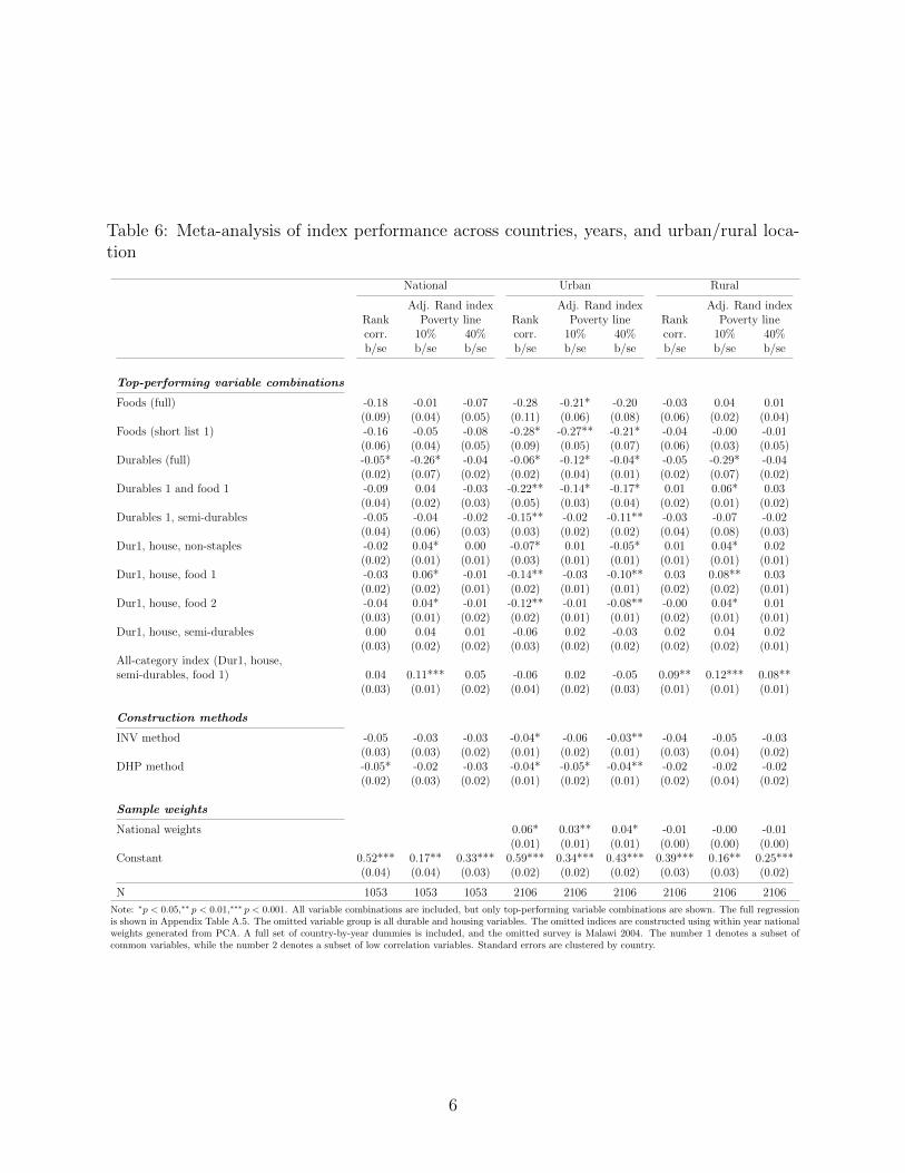
Table 6: Meta-analysis of index performance across countries, years, and urban/rural loca-tion

National Urban Rural

Adj. Rand index Adj. Rand index Adj. Rand indexRank Poverty line Rank Poverty line Rank Poverty linecorr. 10% 40% corr. 10% 40% corr. 10% 40%b/se b/se b/se b/se b/se b/se b/se b/se b/se

Top-performing variable combinations

Foods (full) -0.18 -0.01 -0.07 -0.28 -0.21* -0.20 -0.03 0.04 0.01(0.09) (0.04) (0.05) (0.11) (0.06) (0.08) (0.06) (0.02) (0.04)

Foods (short list 1) -0.16 -0.05 -0.08 -0.28* -0.27** -0.21* -0.04 -0.00 -0.01(0.06) (0.04) (0.05) (0.09) (0.05) (0.07) (0.06) (0.03) (0.05)

Durables (full) -0.05* -0.26* -0.04 -0.06* -0.12* -0.04* -0.05 -0.29* -0.04(0.02) (0.07) (0.02) (0.02) (0.04) (0.01) (0.02) (0.07) (0.02)

Durables 1 and food 1 -0.09 0.04 -0.03 -0.22** -0.14* -0.17* 0.01 0.06* 0.03(0.04) (0.02) (0.03) (0.05) (0.03) (0.04) (0.02) (0.01) (0.02)

Durables 1, semi-durables -0.05 -0.04 -0.02 -0.15** -0.02 -0.11** -0.03 -0.07 -0.02(0.04) (0.06) (0.03) (0.03) (0.02) (0.02) (0.04) (0.08) (0.03)

Dur1, house, non-staples -0.02 0.04* 0.00 -0.07* 0.01 -0.05* 0.01 0.04* 0.02(0.02) (0.01) (0.01) (0.03) (0.01) (0.01) (0.01) (0.01) (0.01)

Dur1, house, food 1 -0.03 0.06* -0.01 -0.14** -0.03 -0.10** 0.03 0.08** 0.03(0.02) (0.02) (0.01) (0.02) (0.01) (0.01) (0.02) (0.02) (0.01)

Dur1, house, food 2 -0.04 0.04* -0.01 -0.12** -0.01 -0.08** -0.00 0.04* 0.01(0.03) (0.01) (0.02) (0.02) (0.01) (0.01) (0.02) (0.01) (0.01)

Dur1, house, semi-durables 0.00 0.04 0.01 -0.06 0.02 -0.03 0.02 0.04 0.02(0.03) (0.02) (0.02) (0.03) (0.02) (0.02) (0.02) (0.02) (0.01)

All-category index (Dur1, house,semi-durables, food 1) 0.04 0.11*** 0.05 -0.06 0.02 -0.05 0.09** 0.12*** 0.08**

(0.03) (0.01) (0.02) (0.04) (0.02) (0.03) (0.01) (0.01) (0.01)

Construction methods

INV method -0.05 -0.03 -0.03 -0.04* -0.06 -0.03** -0.04 -0.05 -0.03(0.03) (0.03) (0.02) (0.01) (0.02) (0.01) (0.03) (0.04) (0.02)

DHP method -0.05* -0.02 -0.03 -0.04* -0.05* -0.04** -0.02 -0.02 -0.02(0.02) (0.03) (0.02) (0.01) (0.02) (0.01) (0.02) (0.04) (0.02)

Sample weights

National weights 0.06* 0.03** 0.04* -0.01 -0.00 -0.01(0.01) (0.01) (0.01) (0.00) (0.00) (0.00)

Constant 0.52*** 0.17** 0.33*** 0.59*** 0.34*** 0.43*** 0.39*** 0.16** 0.25***(0.04) (0.04) (0.03) (0.02) (0.02) (0.02) (0.03) (0.03) (0.02)

N 1053 1053 1053 2106 2106 2106 2106 2106 2106

Note: ∗p < 0.05,∗∗ p < 0.01,∗∗∗ p < 0.001. All variable combinations are included, but only top-performing variable combinations are shown. The full regressionis shown in Appendix Table A.5. The omitted variable group is all durable and housing variables. The omitted indices are constructed using within year nationalweights generated from PCA. A full set of country-by-year dummies is included, and the omitted survey is Malawi 2004. The number 1 denotes a subset ofcommon variables, while the number 2 denotes a subset of low correlation variables. Standard errors are clustered by country.

6

Appendix (not for publication)

7

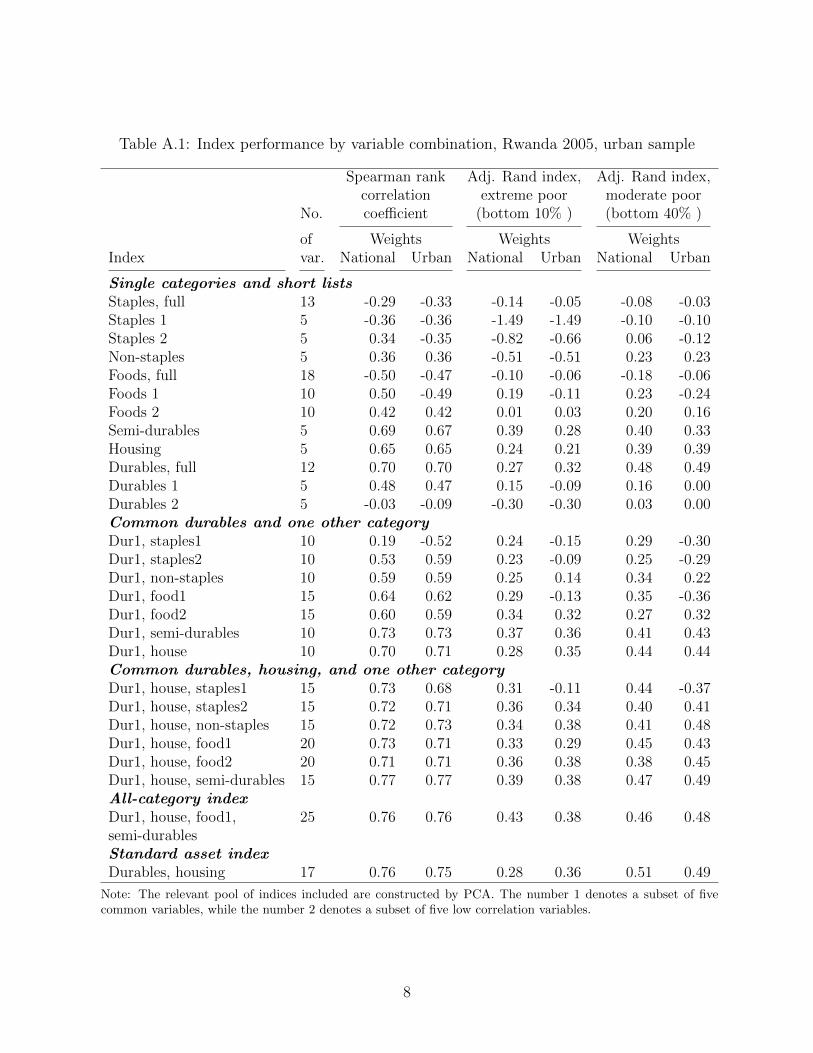
Table A.1: Index performance by variable combination, Rwanda 2005, urban sample

Spearman rank Adj. Rand index, Adj. Rand index,correlation extreme poor moderate poor

No. coefficient (bottom 10% ) (bottom 40% )

of Weights Weights WeightsIndex var. National Urban National Urban National Urban

Single categories and short listsStaples, full 13 -0.29 -0.33 -0.14 -0.05 -0.08 -0.03Staples 1 5 -0.36 -0.36 -1.49 -1.49 -0.10 -0.10Staples 2 5 0.34 -0.35 -0.82 -0.66 0.06 -0.12Non-staples 5 0.36 0.36 -0.51 -0.51 0.23 0.23Foods, full 18 -0.50 -0.47 -0.10 -0.06 -0.18 -0.06Foods 1 10 0.50 -0.49 0.19 -0.11 0.23 -0.24Foods 2 10 0.42 0.42 0.01 0.03 0.20 0.16Semi-durables 5 0.69 0.67 0.39 0.28 0.40 0.33Housing 5 0.65 0.65 0.24 0.21 0.39 0.39Durables, full 12 0.70 0.70 0.27 0.32 0.48 0.49Durables 1 5 0.48 0.47 0.15 -0.09 0.16 0.00Durables 2 5 -0.03 -0.09 -0.30 -0.30 0.03 0.00Common durables and one other categoryDur1, staples1 10 0.19 -0.52 0.24 -0.15 0.29 -0.30Dur1, staples2 10 0.53 0.59 0.23 -0.09 0.25 -0.29Dur1, non-staples 10 0.59 0.59 0.25 0.14 0.34 0.22Dur1, food1 15 0.64 0.62 0.29 -0.13 0.35 -0.36Dur1, food2 15 0.60 0.59 0.34 0.32 0.27 0.32Dur1, semi-durables 10 0.73 0.73 0.37 0.36 0.41 0.43Dur1, house 10 0.70 0.71 0.28 0.35 0.44 0.44Common durables, housing, and one other categoryDur1, house, staples1 15 0.73 0.68 0.31 -0.11 0.44 -0.37Dur1, house, staples2 15 0.72 0.71 0.36 0.34 0.40 0.41Dur1, house, non-staples 15 0.72 0.73 0.34 0.38 0.41 0.48Dur1, house, food1 20 0.73 0.71 0.33 0.29 0.45 0.43Dur1, house, food2 20 0.71 0.71 0.36 0.38 0.38 0.45Dur1, house, semi-durables 15 0.77 0.77 0.39 0.38 0.47 0.49All-category indexDur1, house, food1, 25 0.76 0.76 0.43 0.38 0.46 0.48semi-durablesStandard asset indexDurables, housing 17 0.76 0.75 0.28 0.36 0.51 0.49

Note: The relevant pool of indices included are constructed by PCA. The number 1 denotes a subset of fivecommon variables, while the number 2 denotes a subset of five low correlation variables.

8

Table A.2: Index performance by variable combination, Rwanda 2005, rural sample

Spearman rank Adj. Rand index, Adj. Rand index,correlation extreme poor moderate poor

No. coefficient (bottom 10% ) (bottom 40% )

of Weights Weights WeightsIndex var. National Rural National Rural National Rural

Single categories and short listsStaples, full 13 0.26 0.29 0.06 0.07 0.18 0.20Staples 1 5 0.21 0.04 -0.02 -0.23 0.14 0.05Staples 2 5 -0.02 0.19 -0.80 -0.48 -0.02 0.13Non-staples 5 0.24 0.24 -2.91 -2.91 -0.03 -0.03Foods, full 18 0.13 0.32 0.02 0.08 0.13 0.21Foods 1 10 0.01 0.33 -0.33 -0.03 -0.09 0.06Foods 2 10 0.18 0.27 -0.55 -0.02 0.00 0.17Semi-durables 5 0.45 0.45 0.10 0.10 0.28 0.28Housing 5 0.31 0.18 0.13 0.13 0.20 0.09Durables, full 12 0.46 0.47 -0.55 -0.86 0.29 0.29Durables 1 5 0.43 0.43 -0.88 0.07 0.30 0.30Durables 2 5 0.37 0.37 0.02 0.02 0.10 0.10Common durables and one other categoryDur1, staples1 10 0.46 0.45 0.00 0.17 0.19 0.33Dur1, staples2 10 0.45 0.45 0.03 0.06 0.29 0.30Dur1, non-staples 10 0.47 0.46 -0.62 0.10 0.29 0.29Dur1, food1 15 0.38 0.48 0.01 0.18 0.18 0.33Dur1, food2 15 0.46 0.48 0.09 0.08 0.28 0.32Dur1, semi-durables 10 0.53 0.52 0.14 0.14 0.33 0.33Dur1, house 10 0.47 0.45 0.17 0.18 0.32 0.32Common durables, housing, and one other categoryDur1, house, staples1 15 0.42 0.48 0.06 0.21 0.23 0.35Dur1, house, staples2 15 0.48 0.48 0.12 0.19 0.28 0.34Dur1, house, non-staples 15 0.51 0.48 0.15 0.21 0.33 0.33Dur1, house, food1 20 0.44 0.51 0.07 0.21 0.23 0.36Dur1, house, food2 20 0.50 0.50 0.11 0.20 0.29 0.35Dur1, house, semi-durables 15 0.55 0.54 0.22 0.23 0.34 0.35All-category indexDur1, house, food1, 25 0.53 0.58 0.14 0.24 0.31 0.38semi-durablesStandard asset indexDurables, housing 17 0.49 0.50 0.17 0.16 0.32 0.33

Note: The relevant pool of indices included are constructed by PCA. The number 1 denotes a subset of fivecommon variables, while the number 2 denotes a subset of five low correlation variables.

9

Table A.3: Highest performing variable combinations for Spearman rank correlations, urbanand rural samples from second and third waves

Spearman rank correlations

First highest Second highestcombination Value combination Value

Malawi

Rural, 2010 Foods (full) 0.63 All 0.60Urban, 2010 All 0.67 Foods (full) 0.67

Uganda

Rural, 2009 All 0.54 Foods (full) 0.50Urban, 2009 Dur1, house, food2 0.65 Dur1, house, non-staples 0.65Rural, 2010 All 0.61 Dur1, house, semi-dur 0.55Urban, 2010 Dur1, house, semi-dur 0.64 All 0.63

Rwanda

Rural, 2005 Dur1, house, semi-dur 0.55 All 0.53Urban, 2005 Dur1, house, semi-dur 0.77 All 0.76Rural, 2010 All 0.57 Dur1, house, semi-dur 0.54Urban, 2010 All 0.80 Dur, house 0.79Tanzania

Rural, 2010 All 0.59 Dur1, house, food1 0.57Urban, 2010 Dur, house 0.65 Durables (full) 0.57

Ghana

Rural, 1998 All 0.50 Dur1, house, food1 0.48Urban, 1998 Dur, house 0.44 Durables (full) 0.43Rural, 2005 All 0.54 Dur1, house, food2 0.52Urban, 2005 Dur, house 0.52 Durables (full) 0.49

Note: The relevant pool of indices included are constructed using national weights generatedfrom PCA. The number 1 denotes a subset of five common variables, while the number 2 denotesa subset of five low correlation variables. “Dur, house” refers to the complete list of durable andhousing variables. “All” refers to the combination of common durables, housing, semi-durables,common staple foods, and non-staples.

10

Tab

leA

.4:

Hig

hes

tp

erfo

rmin

gva

riab

leco

mbin

atio

ns

for

adju

sted

Ran

din

dex

,urb

anan

dru

ral

sam

ple

sfr

omse

cond

and

thir

dw

aves

Adju

sted

Ran

din

dex

,ex

trem

ep

oor

(bot

tom

10%

)A

dju

sted

Ran

din

dex

,m

oder

ate

poor

(bot

tom

40%

)

Fir

sthig

hes

tSec

ond

hig

hes

tF

irst

hig

hes

tSec

ond

hig

hes

tco

mbin

atio

nV

alue

com

bin

atio

nV

alue

com

bin

atio

nV

alue

com

bin

atio

nV

alue

Malawi

Rura

l,20

10A

ll0.

28D

ur1

,fo

od1

0.25

Foods

(full)

0.44

All

0.44

Urb

an,

2010

All

0.42

Foods

(full)

0.38

All

0.50

Foods

(full)

0.48

Uganda

Rura

l,20

09A

ll0.

28D

ur1

,se

mi-

dur

0.26

All

0.36

Dur1

,fo

od2

0.33

Urb

an,

2009

All

0.58

Dur1

,hou

se,

sem

i-dur

0.55

Dur1

,hou

se,

stap

le2

0.47

Dur,

hou

se0.

45R

ura

l,20

10A

ll0.

29D

ur1

,fo

od1

0.25

All

0.45

Dur1

,hou

se,

food1

0.39

Urb

an,

2010

All

0.52

Dur1

,hou

se,

sem

i-dur

0.49

Dur,

hou

se0.

46D

ur1

,hou

se,

sem

i-dur

0.46

Rwanda

Rura

l,20

05D

ur1

,hou

se,

sem

i-dur

0.28

Dur1

,se

mi-

dur

0.26

Dur1

,hou

se,

sem

i-dur

0.37

Dur1

,se

mi-

dur

0.36

Urb

an,

2005

Dur1

,hou

se,

non

-sta

ple

s0.

32D

ur1

,hou

se,

sem

i-dur

0.32

Dur1

,hou

se,

sem

i-dur

0.63

All

0.59

Rura

l,20

10A

ll0.

25D

ur1

,hou

se,

sem

i-dur

0.23

All

0.38

Dur1

,hou

se,

sem

i-dur

0.36

Urb

an,

2010

All

0.38

Dur1

,hou

se,

food2

0.36

All

0.68

Dur1

,hou

se,

sem

i-dur

0.64

Tanza

nia

Rura

l,20

10A

ll0.

29D

ur1

,hou

se,

food1

0.29

All

0.39

Sta

ple

s(f

ull)

0.38

Urb

an,

2010

All

0.35

Dur1

,hou

se,

stap

le1

0.35

Dur,

hou

se0.

48D

ur1

,hou

se,

stap

le2

0.43

Ghana

Rura

l,19

98D

ur1

,hou

se,

food1

0.38

All

0.36

Dur1

,fo

od1

0.41

All

0.41

Urb

an,

1998

Dur1

,hou

se,

non

-sta

ple

s0.

33D

ur,

hou

se0.

32D

ur,

hou

se0.

32D

ura

ble

s(f

ull)

0.31

Rura

l,20

05A

ll0.

40D

ur1

,hou

se,

food1

0.39

All

0.31

Dur1

,hou

se,

food1

0.29

Urb

an,

2005

Dur1

,hou

se,

food2

0.33

Dur1

,hou

se,

stap

le1

0.30

Dur,

hou

se0.

36D

ura

ble

s(f

ull)

0.35

Not

e:T

he

rele

vant

pool

ofin

dic

esin

cluded

are

const

ruct

edusi

ng

nat

ional

wei

ghts

gener

ated

from

PC

A.

The

num

ber

1den

ote

sa

subse

tof

five

com

mon

vari

able

s,w

hile

the

num

ber

2den

otes

asu

bse

tof

five

low

corr

elat

ion

vari

able

s.“D

ur,

hou

se”

refe

rsto

the

com

ple

telist

ofdura

ble

and

hou

sing

vari

able

s.“A

ll”

refe

rsto

the

com

bin

ati

on

of

com

mon

dura

ble

s,hou

sing,

sem

i-dura

ble

s,co

mm

on

stap

lefo

ods,

and

non

-sta

ple

s.

11

Table A.5: Meta-analysis of index performance across countries, years, and urban/rurallocation

National Urban Rural

Adj. Rand index Adj. Rand index Adj. Rand indexRank Poverty line Rank Poverty line Rank Poverty linecorr. 10% 40% corr. 10% 40% corr. 10% 40%b/se b/se b/se b/se b/se b/se b/se b/se b/se

Variable combinations

Single categories and short listsStaples (full) -0.26* -0.10* -0.13 -0.37* -0.30** -0.26* -0.10 -0.05* -0.05

(0.08) (0.03) (0.05) (0.11) (0.06) (0.08) (0.05) (0.01) (0.03)Staples (short list1) -0.36** -0.18** -0.20** -0.52** -0.50** -0.42** -0.15* -0.11*** -0.09

(0.08) (0.03) (0.03) (0.10) (0.07) (0.08) (0.05) (0.01) (0.04)Staples (short list2) -0.48** -0.97** -0.35** -0.51*** -1.06** -0.39*** -0.35*** -0.92** -0.27***

(0.07) (0.20) (0.05) (0.05) (0.13) (0.03) (0.04) (0.19) (0.03)Non-staples -0.15* -0.72 -0.11 -0.20* -0.48* -0.16* -0.07 -0.79 -0.07

(0.05) (0.45) (0.04) (0.07) (0.15) (0.04) (0.05) (0.49) (0.06)Foods (full) -0.18 -0.01 -0.07 -0.28 -0.21* -0.20 -0.03 0.04 0.01

(0.09) (0.04) (0.05) (0.11) (0.06) (0.08) (0.06) (0.02) (0.04)Foods (short list 1) -0.16 -0.05 -0.08 -0.28* -0.27** -0.21* -0.04 -0.00 -0.01

(0.06) (0.04) (0.05) (0.09) (0.05) (0.07) (0.06) (0.03) (0.05)Foods (short list 2) -0.19* -0.21 -0.12 -0.24* -0.28*** -0.17* -0.10 -0.13 -0.06

(0.06) (0.08) (0.04) (0.07) (0.03) (0.05) (0.05) (0.05) (0.05)Semi-durables -0.10 -0.42* -0.08 -0.20* -0.22 -0.20* -0.05 -0.48 -0.09

(0.06) (0.11) (0.03) (0.05) (0.08) (0.05) (0.03) (0.18) (0.03)Housing -0.12** -0.29* -0.10* -0.11* -0.14*** -0.10** -0.12* -0.35 -0.10*

(0.02) (0.10) (0.03) (0.04) (0.01) (0.01) (0.03) (0.15) (0.03)Durables (full) -0.05* -0.26* -0.04 -0.06* -0.12* -0.04* -0.05 -0.29* -0.04

(0.02) (0.07) (0.02) (0.02) (0.04) (0.01) (0.02) (0.07) (0.02)Durables (short list 1) -0.20** -0.45* -0.12* -0.29** -0.27** -0.21** -0.14* -0.48* -0.10

(0.03) (0.12) (0.03) (0.05) (0.04) (0.04) (0.04) (0.12) (0.04)Durables (short list 2) -0.26** -0.73* -0.23** -0.30* -0.64 -0.27** -0.17** -0.65** -0.17**

(0.04) (0.19) (0.04) (0.08) (0.24) (0.06) (0.03) (0.13) (0.02)Common durables and one other categoryDurables 1, staples 1 -0.19*** -0.00 -0.10** -0.38** -0.17** -0.27** -0.06* 0.02 -0.02

(0.02) (0.02) (0.02) (0.06) (0.03) (0.05) (0.01) (0.02) (0.01)Durables 1, staples 2 -0.23* -0.10 -0.13* -0.30*** -0.19** -0.21*** -0.15* -0.10 -0.08*

(0.05) (0.05) (0.03) (0.02) (0.03) (0.02) (0.04) (0.05) (0.03)Durables 1 and non-staples -0.08 -0.09 -0.03 -0.14** -0.09* -0.11** -0.02 -0.10 0.00

(0.03) (0.06) (0.03) (0.02) (0.02) (0.02) (0.02) (0.06) (0.02)Durables 1 and food 1 -0.09 0.04 -0.03 -0.22** -0.14* -0.17* 0.01 0.06* 0.03

(0.04) (0.02) (0.03) (0.05) (0.03) (0.04) (0.02) (0.01) (0.02)Durables 1 and food 2 -0.11 0.01 -0.05 -0.18** -0.10* -0.13** -0.03 0.02 -0.00

(0.04) (0.02) (0.03) (0.04) (0.03) (0.02) (0.03) (0.02) (0.02)Durables 1, semi-durables -0.05 -0.04 -0.02 -0.15** -0.02 -0.11** -0.03 -0.07 -0.02

(0.04) (0.06) (0.03) (0.03) (0.02) (0.02) (0.04) (0.08) (0.03)Durables 1, housing -0.06* -0.01* -0.03* -0.09* -0.04* -0.07* -0.04*** -0.01 -0.02***

(0.01) (0.00) (0.01) (0.02) (0.01) (0.02) (0.00) (0.01) (0.00)

Note: Continued on next page.

12

Continued from previous page

National Urban Rural

Adj. Rand index Adj. Rand index Adj. Rand indexRank Poverty line Rank Poverty line Rank Poverty linecorr. 10% 40% corr. 10% 40% corr. 10% 40%b/se b/se b/se b/se b/se b/se b/se b/se b/se

Common durables, housing, and one other categoryDur1, house, staples 1 -0.06** 0.04* -0.03*** -0.19* -0.05* -0.13* -0.01 0.05* 0.00

(0.01) (0.01) (0.00) (0.04) (0.01) (0.03) (0.01) (0.01) (0.01)Dur1, house, staples 2 -0.08* -0.00 -0.04* -0.14** -0.04 -0.08** -0.05** 0.01 -0.02**

(0.02) (0.01) (0.01) (0.02) (0.02) (0.01) (0.01) (0.01) (0.00)Dur1, house, non-staples -0.02 0.04* 0.00 -0.07* 0.01 -0.05* 0.01 0.04* 0.02

(0.02) (0.01) (0.01) (0.03) (0.01) (0.01) (0.01) (0.01) (0.01)Dur1, house, food 1 -0.03 0.06* -0.01 -0.14** -0.03 -0.10** 0.03 0.08** 0.03

(0.02) (0.02) (0.01) (0.02) (0.01) (0.01) (0.02) (0.02) (0.01)Dur1, house, food 2 -0.04 0.04* -0.01 -0.12** -0.01 -0.08** -0.00 0.04* 0.01

(0.03) (0.01) (0.02) (0.02) (0.01) (0.01) (0.02) (0.01) (0.01)Dur1, house, semi-durables 0.00 0.04 0.01 -0.06 0.02 -0.03 0.02 0.04 0.02

(0.03) (0.02) (0.02) (0.03) (0.02) (0.02) (0.02) (0.02) (0.01)All-category indexDur1, house, food 1, 0.04 0.11*** 0.05 -0.06 0.02 -0.05 0.09** 0.12*** 0.08**semi-durables (0.03) (0.01) (0.02) (0.04) (0.02) (0.03) (0.01) (0.01) (0.01)Construction methods

INV method -0.05 -0.03 -0.03 -0.04* -0.06 -0.03** -0.04 -0.05 -0.03(0.03) (0.03) (0.02) (0.01) (0.02) (0.01) (0.03) (0.04) (0.02)

DHP method -0.05* -0.02 -0.03 -0.04* -0.05* -0.04** -0.02 -0.02 -0.02(0.02) (0.03) (0.02) (0.01) (0.02) (0.01) (0.02) (0.04) (0.02)

Sample weights

National weights 0.06* 0.03** 0.04* -0.01 -0.00 -0.01(0.01) (0.01) (0.01) (0.00) (0.00) (0.00)

Survey indicators

Ghana 1991 -0.10*** -0.02*** -0.08*** -0.22*** -0.16*** -0.17*** -0.09*** 0.00*** -0.07***(0.00) (0.00) (0.00) (0.00) (0.00) (0.00) (0.00) (0.00) (0.00)

Ghana 1998 -0.03*** 0.05*** -0.01*** -0.16*** -0.12*** -0.14*** -0.01*** 0.04*** 0.02***(0.00) (0.00) (0.00) (0.00) (0.00) (0.00) (0.00) (0.00) (0.00)

Ghana 2005 -0.07*** -0.02*** -0.06*** -0.16*** -0.14*** -0.14*** -0.05*** 0.01*** -0.06***(0.00) (0.00) (0.00) (0.00) (0.00) (0.00) (0.00) (0.00) (0.00)

Malawi 2010 0.13*** 0.03*** 0.09*** 0.02*** 0.03*** 0.02*** 0.12*** 0.00*** 0.09***(0.00) (0.00) (0.00) (0.00) (0.00) (0.00) (0.00) (0.00) (0.00)

Rwanda 2000 0.09*** -0.09*** 0.03*** -0.08*** -0.05*** -0.08*** 0.06*** -0.07*** 0.05***(0.00) (0.00) (0.00) (0.00) (0.00) (0.00) (0.00) (0.00) (0.00)

Rwanda 2005 0.08*** -0.06*** 0.03*** 0.01*** -0.05*** 0.02*** 0.08*** -0.07*** 0.05***(0.00) (0.00) (0.00) (0.00) (0.00) (0.00) (0.00) (0.00) (0.00)

Rwanda 2010 0.06*** -0.03*** 0.01*** 0.09*** -0.03*** 0.08*** 0.05*** -0.05*** 0.02***(0.00) (0.00) (0.00) (0.00) (0.00) (0.00) (0.00) (0.00) (0.00)

Tanzania 2008 0.15*** 0.09*** 0.10*** -0.03*** 0.04*** -0.02*** 0.09*** 0.04*** 0.07***(0.00) (0.00) (0.00) (0.00) (0.00) (0.00) (0.00) (0.00) (0.00)

Tanzania 2010 0.15*** 0.14*** 0.11*** -0.03*** 0.03*** -0.00*** 0.14*** 0.08*** 0.09***(0.00) (0.00) (0.00) (0.00) (0.00) (0.00) (0.00) (0.00) (0.00)

Uganda 2005 0.13*** 0.07*** 0.11*** -0.04*** -0.07*** -0.09*** 0.15*** 0.02*** 0.10***(0.00) (0.00) (0.00) (0.00) (0.00) (0.00) (0.00) (0.00) (0.00)

Uganda 2009 0.11*** 0.06*** 0.05*** 0.01*** 0.08*** -0.01*** 0.10*** 0.07*** 0.06***(0.00) (0.00) (0.00) (0.00) (0.00) (0.00) (0.00) (0.00) (0.00)

Uganda 2010 0.11*** 0.05*** 0.06*** 0.04*** -0.07*** 0.01*** 0.11*** 0.07*** 0.09***(0.00) (0.00) (0.00) (0.00) (0.00) (0.00) (0.00) (0.00) (0.00)

Constant 0.52*** 0.17** 0.33*** 0.59*** 0.34*** 0.43*** 0.39*** 0.16** 0.25***(0.04) (0.04) (0.03) (0.02) (0.02) (0.02) (0.03) (0.03) (0.02)

N 1053 1053 1053 2106 2106 2106 2106 2106 2106

Note: ∗p < 0.05,∗∗ p < 0.01,∗∗∗ p < 0.001. The omitted variable group is all durable and housing variables. The omitted indices are constructedusing within year national weights generated from PCA. The omitted survey is Malawi 2004. The number 1 denotes a subset of common variables,while the number 2 denotes a subset of low correlation variables. Standard errors are clustered by country.13