The Pennsylvania State University - Amazon Web … Pennsylvania State University The Graduate School...

The Pennsylvania State University

The Graduate School

Department of Ecosystem Science and Management

MONITORING WILD RING-NECKED PHEASANT

POPULATION RESTORATION IN PENNSYLVANIA

A Thesis in

Wildlife and Fisheries Science

by

Lacey Taylor Williamson

2017 Lacey Taylor Williamson

Submitted in Partial Fulfillment

of the Requirements

for the Degree of

Master of Science

December 2017

ii

The thesis of Lacey Taylor Williamson was reviewed and approved* by the following:

W. David Walter

Adjunct Assistant Professor of Wildlife Ecology

Thesis Co-Adviser

Duane R. Diefenbach

Adjunct Professor of Wildlife Ecology

Thesis Co-Adviser

Matt R. Marshall

Adjunct Assistant Professor of Wildlife Conservation

Michael G. Messina

Professor of Ecosystem Science and Management

Head of the Department of Ecosystem Science and Management

*Signatures are on file in the Graduate School

iii

ABSTRACT

Ring-necked pheasants (Phasianus colchicus) are a non-native species that has become

naturalized and a popular game bird in the United States. The population in Pennsylvania

has been declining since the 1970s despite stocking and habitat restoration efforts. One of

the management objectives of the Pennsylvania Game Commission is to provide quality

pheasant hunting which requires restoration of the wild pheasant population so that it is

naturally reproducing and able to withstand hunting pressure. The current best potential

habitat for pheasants within the state was identified and 4 wild pheasant recovery areas

(WPRAs) were created to monitor pheasant restoration efforts. At these areas, it was

illegal to release stocked pheasants, hunt and harvest either sex, or train dogs. Wild-

trapped pheasants from South Dakota and Montana were released at the study areas to

ensure there would be an adequate founding population for restoration purposes. The

Pennsylvania Game Commission set objectives for a density of 3.86 female

pheasants/km2 and that would be adequate for maintaining a sustainable population with

hunting pressure. To assess the success of the project and aid in future management

decisions, we explored methods of estimating the density by incorporating multiple

detection probabilities and a model for predicting potential female pheasant density based

on micro-habitat data.

As opposed to requiring multiple years of monitoring to obtain population trends

using indices of abundance, we used crowing counts and adjusted for detection

probabilities to estimate density at each of 12 study areas from 2013 to 2016. Our density

estimates were adjusted for the probability a male pheasant crowed in a 3-minute survey

iv

period, the probability an observer was able to detect a pheasant given that it crowed, and

the probability of flushing a male pheasant. We found the probability a male crowed in

the survey period to decrease linearly during the breeding period (21 April–23 May) from

0.659 to 0.464. The probability of detecting a crowing pheasant at 0.80 km was >0,

indicating that there was no distance at which it was reasonable to assume no birds could

be detected. Instead, the effective area was used and is robust to choice of radius.

Because the male pheasants are recorded during the crowing counts and female densities

are required to meet objectives, we estimated the probability of flushing a male pheasant

to be 0.495 yielding an almost 1:1 sex ratio. Only one of 12 study areas achieved the

female density goal of 3.86 females/km2 from 2013 to 2016. The methods used to obtain

these density estimates simplified the crowing count protocol and can easily be used and

adjusted for other species, detection probabilities, or survey areas to estimate density.

To assess habitat or landscape composition at the WPRAs, we conducted a micro-

habitat analysis by identifying all vegetation types within a 0.56 km radius of the survey

point (hereafter referred to as survey circle) resulting in digitized maps of micro-habitat

within a survey circle. Our objective was to create a model that would be able to predict

potential female pheasant densities based on proportion of habitat type in a survey circle.

We had 37 vegetation types that were combined into 8 habitat types a priori and used

these as independent variables in our predictive models. We used our methods of

estimating pheasant densities (Chapter 2) to estimate female density at the survey circle

to be used as the dependent variable. For the model, we used 2 years of micro-habitat

data (2013–2014) and density estimates (2014–2015). We estimated that female pheasant

densities were influenced most by the proportion of idle grasses and forest. We found the

v

proportion of idle grass to positively influence pheasant densities, while forest had a

negative influence. This model will be important for improving habitat to meet a desired

pheasant density goal by allowing managers to make recommendations for quantity and

proportions of habitat needed to achieve desired pheasant density goals.

Only one study area, Washingtonville West, was successful in meeting the density

goal of 3.86 female pheasants/km2, while all other study areas did not exceed a density of

2 females/km2. Washingtonville West had the lowest average proportion of forest in a

survey circle of any study area. From 2013 to 2015, the average proportion of forest

ranged from 4.3% to 9.3% at Washingtonville West, compared to an overall average at

all the WPRAs ranging from 15.6% to 17.6%. Given that roughly 60% of the overall

landscape in Pennsylvania is forested, the WPRAs represent a small section of the state

that is potentially suitable pheasant habitat. Even at this suitable habitat, we only

achieved a self-sustainable pheasant population that can withstand hunting pressure at

one study area which had <10% forest. Because forest has a negative effect on pheasant

densities and so much of the Pennsylvania landscape is forested, it will be difficult to

locate enough suitable habitat to support sustainable pheasant populations in order to

provide hunting opportunities across the state

vi

TABLE OF CONTENTS

LIST OF FIGURES ........................................................................................................ vii

LIST OF TABLES ......................................................................................................... viii

ACKNOWLEDGMENTS ............................................................................................... ix

Chapter 1 The current status of ring-necked pheasants in a forest-dominated landscape:

where do we go from here? ...................................................................................... 1

LITERATURE CITED ............................................................................................ 9

Chapter 2 Estimating detection probability for bird population density estimates ................ 17


Chapter 3 Modeling potential habitat for restoration of ring-necked pheasants .................... 48


Chapter 4 The future of ring-necked pheasants in Pennsylvania ......................................... 72

LITERATURE CITED ..................................................................................... 75

vii

LIST OF FIGURES

Figure 1-1.The proportion of land (%) in agriculture and forest in Pennsylvania (U.S.

Bureau of the Census 1940;1967;1983, Oswalt et al. 2014, U.S. Department of

Agriculture 2014), 1920–2012. ........................................................................................ 15

Figure 2-1. The locations of wild pheasant recovery areas (WPRAs) and county outlines

in Pennsylvania, 2013–2016. ........................................................................................... 39

Figure 2-2. Raw probability that a pheasant equipped with a radiotransmitter ( 21n )

crowed during a 3-minute survey period based on calendar day plotted with the line

of best fit, Pennsylvania, 2014–2015. .............................................................................. 39

Figure 3-1. An example of a survey circle (0.56 km radius) with the different habitat

patches categorized according to the Anderson-level land use (A; Anderson 1976)

and the same survey circle combined using our 8 habitat categories (B). ....................... 67

Figure 3-2. The predicted female pheasant density (female pheasants/km2) plotted against

the estimated female pheasant density (female pheasants/km2) with the line of best

fit (solid) and a one-to-one ratio (dashed). ....................................................................... 67

viii

LIST OF TABLES

Table 2-1. Number of survey points at which crowing counts were conducted and the size

of the wild pheasant recovery areas (WPRAs), Pennsylvania, 2013–2016. .................... 40

Table 2-2. Year of initial reintroduction, cumulative number of translocated ring-necked

pheasants (only females are reported), and resulting densities (female

pheasants/km2) of released pheasants on wild pheasant recovery areas (WPRAs) and

study areas within each WPRA. No pheasants were released at the Washingtonville

South or North Franklin study areas. Densities represent the number of released

female pheasants over a study area and are not adjusted for detection probabilities,

Pennsylvania, 2007–2014. ............................................................................................... 41

Table 2-3. Model selection for linear mixed effects models (each individual bird was

treated as a random effect) estimating the probability that a male pheasant will crow

≥1 time during a 3-minute period ( AP ), Pennsylvania, 2014–2015. ............................... 42

Table 2-4. Model selection for the logistic regression models estimating probability that a

flushed pheasant was male. Variables in parentheses were included as random

effects, Pennsylvania, 2013–2016. ................................................................................... 43

Table 2-5. Density estimates (female pheasants/km2) and standard errors for female

pheasants in the Somerset and Hegins-Gratz wild pheasant recovery areas,

Pennsylvania, 2013–2016. ............................................................................................... 44

Table 2-6. Density estimates (female pheasants/km2) and standard errors for female

pheasants in the Central Susquehanna and Franklin wild pheasant recovery areas,

Pennsylvania, 2013–2016. ............................................................................................... 45

Table 3-1. Survey circles, size of wild pheasant recovery areas (WPRAs) and study areas,

and the average proportion of habitat per survey circle (%). The Conservation

Reserve Enhancement Program (CREP; Farm Service Agency, Washington, D.C.,

USA) habitat proportions were calculated separately and may overlap other

categories, Pennsylvania, 2013–2015. ............................................................................. 68

Table 3-2. Parameters, number of parameters (K), difference in value from the model

with the model having the lowest AICc value (Δ AICc), -2 × log-likelihood, and

weights (wi) for linear mixed effects models estimating female pheasant density

(log(Female Density+1) based on micro-habitat variables in Pennsylvania, 2013–

2015. Study area and circle identification were included in all models as random

effects. .............................................................................................................................. 69

ix

ACKNOWLEDGMENTS

I would like to thank all those who contributed to make this project possible. I thank both

of my advisers, David Walter and Duane Diefenbach, for their support, trust, and

guidance in completing this project. Thank you to my other committee member, Matt

Marshall, for the suggestions and input along the way. A special thanks to Scott Klinger

for all his work on the pheasant restoration project and helping me to find answers that

would be useful for management purposes. Additionally, I’d like to also especially thank

Colleen Delong, Wild Pheasant Project Coordinator in the Pennsylvania Game

Commission (PGC), for nearly 8 years on this project and Jesse Putnam, Habitat Forever,

who coordinated and trapped all wild pheasants in Montana and South Dakota for this

project. I thank Thomas Keller and Ian Gregg from the PGC for their efforts in collecting

data and ensuring I answered the important questions. I appreciate all the hard work and

help from other PGC staff, especially Megan Rake, Brandon Black, Ray Grater, and

Wyatt Knepp. Special thanks to the PA Pheasants Forever chapters, volunteers, and

private landowners. Without these people, the project would not have been possible.

I would also like to thank everyone in the Department of Ecosystem Science and

Management, as well as the Cooperative Research Unit. Their advice, support, and

friendship were crucial to keeping my sanity and spirits up. I really enjoyed my time at

Penn State because of them and I’m so thankful to have found such a large group of

people to call my friends and who I can lean on. I’d also like to thank my friends back

home and my family for their continued support in the pursuit of my dreams.

1

Chapter 1

The current status of ring-necked pheasants in a forest-dominated landscape: where

do we go from here?

Chapter 1 was written in collaboration with Duane R. Diefenbach, Scott R. Klinger, and

W. David Walter. I have included this manuscript on the following pages as formatted for

The Journal of Fish and Wildlife Management.

2

Ring-necked pheasants (Phasianus colchicus) are an iconic and popular game bird. While

pheasants are native to Asia, they have been introduced successfully on multiple

continents and countries, including Europe, North America, Chile, and New Zealand

(Hill and Robertson 1988). The first attempted introduction of pheasants in the United

States occurred in New York in 1733 (Allen 1956), but pheasants were not successfully

recorded as introduced until 1881 in the Willamette Valley of Oregon. Although

pheasants are a non-native species, they have become naturalized (Frey et al. 2003) and

an iconic symbol of the midwestern United States, including being the state bird in South

Dakota. In 1954, the reported pheasant range stretched across the majority of the United

States, with the exception of the Southeast (Edminster 1954).

Pheasants have been declining throughout their range in the United States since

the 1970s (Labisky 1976, Sauer et al. 2017). In the Midwest from 1971 to 1986,

pheasants declined by 33% and collectively by 67% in the rest of the country (Dahlgren

1988). The decline of one of the most popular game birds in the nation has spurred an

increase in pheasant research focusing on aspects that may influence the population, such

as the hardiness of stocked birds (Krauss et al. 1987), survival (Wilson et al. 1992,

Gabbert et al. 1999, Homan et al. 2000), nest success (Haensly et al. 1987, Clark et al.

1999), and habitat use in different seasons (Hill and Ridley 1987, Gatti et al. 1989).

Pheasants are an agriculturally dependent bird (Gerstell 1937, Edminster 1954),

but utilize multiple habitat types throughout the year. During the breeding season,

pheasants will use grasses, pastures, and shrubs for nesting (Hartman and Sheffer 1971,

Schmitz and Clark 1999, Shipley and Scott 2006), but rely on wooded areas, wetlands,

and food plots during the winter months (Hartman and Sheffer 1971, Gabbert et al. 1999,

3

Homan et al. 2000). Much of the pheasant decline is thought to be attributed to habitat

loss and changes in farming practices. Some of the expected reasons contributing to the

declining pheasant populations across the nation are increased monocultures of row crops

(Taylor et al. 1978, Warner 1984), increased use of pesticides reducing the weeds and

insects available for brood rearing (Hill 1985, Rands 1986), early mowing (Hartman et al.

1984, Warner and Etter 1989), and the reduction of a mosaic landscape attributed to

increasing farm and field sizes (Taylor et al. 1978).

To combat the changing landscape and land use, efforts to address pheasant

population declines have focused on improving habitat. The Conservation Reserve

Program (CRP) was created under the Food Security Act of 1985 with the purpose of

paying farmers to remove environmentally sensitive agricultural land from production.

Land was enrolled for 10–15 years and converted from crops or pasture to other

vegetation that provided wildlife cover (Osborn 1993). Habitat created from government

assistance programs, such as the CRP, has benefitted pheasant populations and helped to

maintain crucial habitat for nesting (Haroldson et al. 2006, Nielson et al. 2008, Matthews

et al. 2012).

The northeastern United States is considered less favorable habitat compared to

the western United States (Allen 1956) because of a smaller percentage of the landscape

in agricultural use and the large amount of mountainous and wooded terrain (Rue 1973).

The eastern U.S. has had difficulty maintaining a wild pheasant population that can

sustain hunter harvests (Allen 1956), but Pennsylvania has a rich history of pheasant

hunting. In 1902, Pennsylvania had the first hunting season for pheasants in the

northeastern U.S. (Allen 1956). There were no harvest limits until 1915 when daily,

4

weekly, and seasonal bag limits were established and there was a harvest of 796 birds

(Klinger and Riegner 2008). The Pennsylvania Game Commission (PGC) started

stocking (i.e., pen-reared, artificially propagated, or captive raised birds released to

increase hunting opportunities hereafter referred to as stocked) pheasants in 1915 and

released 2,096 pheasants in the spring, with the intention that they could naturally breed

and be hunted in the fall (Gerstell 1937, Edminster 1954). In the early years that PGC

stocked pheasants, the prediction was that “pheasants will never become established in

Pennsylvania because they cannot stand hard winters and hard hunting both” (Edminster

1954). The hard winters were found not to inhibit population growth and the wild

population soon started to increase (Edminster 1954). In 1936 and 1937, a total of 17,850

banded male pheasants were stocked in fall and spring as part of the PGC’s annual

restocking program. With the spring release of pheasants, the intention for stocked birds

was to supply both a population that could naturally breed in spring and hunting

opportunities during the fall. The fall stocking of banded male pheasants weeks prior to

the hunting season resulted in a reported harvest of 19.1% in 1936 and 24.2% of banded

birds in 1937 (Gerstell 1938).

Stocking efforts and artificial propagation resulted in some individuals surviving

long-term to create a wild pheasant population (Gerstell 1937). The majority of birds

released in the autumn, however, did not survive to the breeding season with the survival

rate of stocked birds <6% within 30-days post-release (Diefenbach et al. 2000). This

survival rate negated the ability of stocked birds to contribute to a self-sustaining wild

pheasant population. Krauss et al. (1987) found that wild-caught male pheasants had

higher survival than stocked males when released at the same time and location, possibly

5

due to stocked birds being less fearful of humans, thus making them more approachable

by predators. To solely provide hunting opportunity, more than 7,916,000 pheasants were

raised and released in Pennsylvania between 1929 and 1998 by the PGC. In 1998, 2.8

million USD was spent on stocked pheasants by the PGC and almost 200,000 pheasants

were released for hunter harvest (Diefenbach et al. 2000). Similar numbers of stocked

pheasants have been released annually to the present day.

In areas that did not support wild pheasants, stocking supplemented the

population to continue providing hunting opportunities. When the pheasant decline

occurred, stocking efforts increased in an attempt to prevent further decline of the

population, but were unsuccessful. It was eventually realized that the stocked pheasants

supplied the majority of hunting opportunities while the wild population continued to

decline (Klinger and Riegner 2008). In recent years, there has been a push to decrease the

amount of stocked pheasants in the state, but still have pheasant hunting opportunities. To

do this, the PGC attempted to restore the wild pheasant population to densities that can

withstand hunter harvest in a sustainable manner. In an effort to stock a hardier bird, the

PGC was hopeful that Sichuan pheasants (Phasianus colchicus strauchi), a subspecies of

ring-necked pheasants, would be better suited to nest in brushy areas instead of the hay

fields relied upon by ring-necked pheasants. Stocking Sichuan and ring-necked pheasants

indicated no differences between the subspecies in habitat selection, survival, or

reproduction in Ohio (Shipley and Scott 2006).

While the increase in research has aided in the management of pheasants,

additional research, specific to Pennsylvania’s land use and ecosystem, was needed to

restore a wild pheasant population to Pennsylvania. The majority of the research on

6

pheasants has occurred in the Midwest, which has a different landscape compared to

Pennsylvania. While previous research offers some insight into the habitat types

pheasants might use in Pennsylvania, there is no indication if an adequate amount of

habitat exists to support pheasant populations that could withstand hunting, if the

population utilizes other habitat types, or possible habitat improvements that could

support pheasant density goals.

By 1937, pheasants had become established in every county within Pennsylvania

(Gerstell 1937). Hartman and Sheffer (1971) classified 63,536 km2 of Pennsylvania,

mainly in the Southeast, as being able to support pheasants and falling into either first,

second, or third class categories. The first class category (21,448 km2) had almost all

natural reproduction and a majority of the pheasant harvest. The second class category

(18,211 km2) accounted for about 20–30% of Pennsylvania’s male harvest with stocked

birds making up about half of the birds harvested. The third class category (23,471 km2)

made up a low proportion of harvest (10%) with about 90% of the harvest from stocked

birds. Latham (1973) reported the western part of Pennsylvania as being prime pheasant

hunting, while Hartman and Sheffer (1971) listed that part of the state as being second or

third class habitat. In 1971, the highest reported pheasant density in Pennsylvania

occurred in the Southeast and exceeded 15.8 females/km2, but by 1986 the highest

reported density in the entire state was 3.9 females/km2 (Dahlgren 1988).

Peak pheasant harvests occurred in 1971 and 1972 with >1.3 million birds

harvested each year (Klinger and Riegner 2008), but annual harvest in 1998 declined to

217,000 (Diefenbach et al. 2000). By the 2000s, pheasant populations in Pennsylvania

had reached the lowest recorded numbers during the Christmas Bird Counts since the

7

1920s (National Audubon Society 2010). There are no records on the number of pheasant

hunters before 1971, but the lowest recorded number of hunters was in 2010 with 71,579

hunters (Johnson 2015).

Since the first pheasant hunting season, the Pennsylvania landscape and land use

has changed. The average size of a farm was lowest in 1935 with 0.34 km2 (U.S. Bureau

of the Census 1967) and highest in 1992 with 0.65 km2 and corresponds with an increase

in monoculture row crops. In 1930, 6.2% of the land at farms was used for grain or seed

corn, 8.9% in 1950, 12.1% in 1974, and 13.0% in 2012 (U.S. Bureau of the Census

1940;1954;1967;1977, U.S. Department of Agriculture 2014). From 1920 to 1977, the

proportion of Pennsylvania that was forested increased from 42.5% to 57.1% and then

stayed relatively stable through 2012 (Figure 1-1; Oswalt et al. 2014). Within this same

time, the proportion of land in agriculture decreased from 59.9% in 1920 to 27.8% in

1974, but leveled out at about 26% from 1987 to 2012 (U.S. Bureau of the Census

1940;1967;1983, U.S. Department of Agriculture 2014). The increase of forested land

and decrease in agriculture appeared to coincide with the pheasant declines in the 1960s

and 1970s. These changes in Pennsylvania may have limited the amount of habitat

available for pheasants and help to explain the population decline.

In 2000, the Conservation Reserve Enhancement Program (CREP), which is a

part of the CRP, was created with the intention that private farmland would be converted

to wildlife habitat and also improve water quality in the Chesapeake Bay watershed

(Klinger and Riegner 2008). Pabian et al. (2015) conducted a study to examine the effect

of CREP habitat on pheasants and found that pheasant abundance was positively

influenced by CREP habitat in south central and southeastern Pennsylvania. It is unclear

8

whether it is possible to enroll enough land in CREP to reverse the pheasant population

decline.

A management objective of the PGC was to provide quality pheasant hunting in

Pennsylvania, which was initially explored at a small spatial scale. In 2002, Pike Run, a

study area in southwestern Pennsylvania, was created and used as an experimental area to

validate restoration as a management option for pheasant. This 125.3 km2 study area was

involved in recent habitat improvement efforts for the first translocations of wild-trapped

pheasants (Klinger and Riegner 2008). A total of 591 wild pheasants from South Dakota

were translocated to the area with 14 pheasants fitted with radiotransmitters to track their

survival (DeLong and Klinger 2008). Fifty percent of birds with a radiotransmitter died

within 2 weeks post-release and 86% died by the end of the nesting season. Crowing

routes and flushing surveys were used to monitor the population and the density was

estimated at 0.77 females/km2 in 2008 (Klinger and Riegner 2008). Because the

estimated density was less than the density goal established by the PGC (3.86

females/km2), the Pike Run study area was closed and reintroduction efforts at this site

ended in 2012 (Klinger et al. 2013).

Although the Pike Run study area did not meet density goals, efforts to locate

other areas that have the ability to support a wild pheasant population continued. Ideal

areas would require minimal habitat improvement initially and would need to meet the

criteria of <20% forest, >50% agriculture, >20% hay, and <10% developed land (Klinger

and Riegner 2008). The PGC created wild pheasant recovery areas (WPRAs) that met the

landscape criteria, were ≥40.5 km2 within contiguous agriculture, and had >5% nesting

cover which may include CREP, hay with delayed mowing, or small grains. Release of

9

stocked birds, pheasant hunting, and dog training were prohibited at WPRAs during

restoration efforts. Due to the low wild pheasant population at the WPRAs and the low

survivability of stocked birds, wild pheasants were trapped in South Dakota and Montana

and released on each WPRA.

At these WPRAs, a more detailed assessment of pheasant density estimates and

habitat composition was needed to assess the success of the areas and the validity of

pheasant restoration in Pennsylvania. A population density goal of 3.86 female

pheasants/km2 was set by the PGC and believed to be necessary to maintaining self-

sustaining pheasant populations that experience hunter harvest (Klinger and Riegner

2008). To assess the ability of having a wild pheasant population in Pennsylvania,

accurate density estimates and knowledge of what habitats are present and being used by

wild pheasants are necessary.

LITERATURE CITED

Allen, D. L. 1956. Pheasants in North America. Stackpole Company.

Clark, W. R., R. A. Schmitz, and T. R. Bogenschutz. 1999. Site selection and nest

success of ring-necked pheasants as a function of location in Iowa landscapes.

The Journal of Wildlife Management 63:976-989.

Dahlgren, R. B. 1988. Distribution and abundance of the ring-necked pheasant in North

America. Pheasants: symptoms of wildlife problems on agricultural lands. North

Central Section of The Wildlife Society, Bloomington, Indiana, USA:29-43.

10

DeLong, C. A., and S. R. Klinger. 2008. Wild ring-necked pheasant restoration in

Pennsylvania. Pennsylvania Game Commission, Bureau of Wildlife Management,

Harrisburg, Pennsylvania, USA.

Diefenbach, D. R., C. F. Riegner, and T. S. Hardisky. 2000. Harvest and reporting rates

of game-farm ring-necked pheasants. Wildlife Society Bulletin (1973-2006)

28:1050-1059.

Edminster, F. C. 1954. American game birds of field and forest: their habits, ecology, and

management. Charles Scribner's Sons, New York.

Frey, S. N., S. Majors, M. R. Conover, T. A. Messmer, and D. L. Mitchell. 2003. Effect

of predator control on ring-necked pheasant populations. Wildlife Society Bulletin

(1973-2006) 31:727-735.

Gabbert, A. E., A. P. Leif, J. R. Purvis, and L. D. Flake. 1999. Survival and habitat use by

ring-necked pheasants during two disparate winters in South Dakota. The Journal

of Wildlife Management 63:711-722.

Gatti, R. C., R. T. Dumke, and C. M. Pils. 1989. Habitat use and movements of female

ring-necked pheasants during fall and winter. The Journal of Wildlife

Management 53:462-475.

Gerstell, R. 1937. The status of the ringneck pheasant in Pennsylvania. Transactions of

the Second North American Wildlife Conference:505-511.

Gerstell, R. 1938. An analysis of the reported returns obtained from the release of 30,000

artificially propagated ringneck pheasants and bobwhite quail. Transactions of the

North American Wildlife Conference 11:724-729.

11

Haensly, T. F., J. A. Crawford, and S. M. Meyers. 1987. Relationships of habitat

structure to nest success of ring-necked pheasants. The Journal of Wildlife


Haroldson, K. J., R. O. Kimmel, M. R. Riggs, and A. H. Berner. 2006. Association of

ring-necked pheasant, gray partridge, and meadowlark abundance to conservation

reserve program grasslands. Journal of Wildlife Management 70:1276-1284.

Hartman, F., R. Fisher, and S. Fletcher. 1984. Delayed haymowing increases pheasant

nesting success in Pennsylvania. Transactions of the Northeast Section of the

Wildlife Society 41:166-179.

Hartman, F., and D. Sheffer. 1971. Population dynamics and hunter harvest of ringnecked

pheasant populations in Pennsylvania’s primary range. Northeast Section of the


Hill, D. 1985. The feeding ecology and survival of pheasant chicks on arable farmland.

Journal of Applied Ecology:645-654.

Hill, D., and M. Ridley. 1987. Sexual segregation in winter, spring dispersal and habitat

use in the pheasant (Phasianus colchicus). Journal of Zoology 212:657-668.

Hill, D., and P. Robertson. 1988. The pheasant. BSP Professional Books.

Homan, H. J., G. M. Linz, and W. J. Bleier. 2000. Winter habitat use and survival of

female ring-necked pheasants (Phasianus colchicus) in southeastern North

Dakota. The American midland naturalist 143:463-480.

Johnson, J. B. 2015. Game take, furtaker, mentored youth hunter, spring turkey hunter,

mentored youth spring turkey hunter surveys. Pennsylvania Game Commission,

Harrisburg, Pennsylvania, USA.

12

Klinger, S., and C. Riegner. 2008. Ring-necked pheasant management plan for

Pennsylvania 2008-2017. Pennsylvania Game Commission, Bureau of Wildlife

Management, Harrisburg, Pennsylvania, USA.

Klinger, S. R., C. A. DeLong, L. J. Crespo, M. M. Rake, and B. P. Black. 2013. Wild

ring-necked pheasant restoration in Pennsylvania. Pennsylvania Game

Commission, Bureau of Wildlife Management, Harrisburg, Pennsylvania, USA.

Krauss, G. D., H. B. Graves, and S. M. Zervanos. 1987. Survival of wild and game-farm

cock pheasants released in Pennsylvania. The Journal of Wildlife Management

51:555-559.

Labisky, R. F. 1976. Midwest pheasant abundance declines. Wildlife Society Bulletin

(1973-2006) 4:182-183.

Latham, R. 1973. Outdoor Guide. The Pittsburgh Press, Pittsburgh, PA, USA.

Matthews, T. W., J. S. Taylor, and L. A. Powell. 2012. Ring‐necked pheasant hens select

managed Conservation Reserve Program grasslands for nesting and brood‐

rearing. The Journal of Wildlife Management 76:1653-1660.

National Audubon Society. 2010. The Christmas bird count historical results.

<http://www.audubon.org/conservation/science/christmas-bird-count/>. Accessed

15 Mar 2016.

Nielson, R. M., L. L. McDonald, J. P. Sullivan, C. Burgess, D. S. Johnson, D. H.

Johnson, S. Bucholtz, S. Hyberg, and S. Howlin. 2008. Estimating the response of

ring-necked pheasants (Phasianus colchicus) to the Conservation Reserve

Program. The Auk 125:434-444.

http://www.audubon.org/conservation/science/christmas-bird-count/%3e

13

Osborn, T. 1993. The Conservation Reserve Program: status, future, and policy options.

Journal of Soil and Water Conservation 48:271-279.

Oswalt, S. N., W. B. Smith, P. D. Miles, and S. A. Pugh. 2014. Forest Resources of the

United States, 2012: a technical document supporting the Forest Service 2010

update of the RPA Assessment.

Pabian, S. E., A. M. Wilson, S. R. Klinger, and M. C. Brittingham. 2015. Pennsylvania's

conservation reserve enhancement program benefits ring‐necked pheasants but

not enough to reverse declines. The Journal of Wildlife Management 79:641-646.

Rands, M. 1986. The survival of gamebird (Galliformes) chicks in relation to pesticide

use on cereals. Ibis 128:57-64.

Rue, L. L. 1973. Game Birds of North America. Outdoor Life, United States.

Sauer, J. R., D. K. Niven, J. E. Hines, D. J. Ziolkowski Jr, K. L. Pardieck, J. E. Fallon,

and W. A. Link. 2017. The North American breeding bird survey, results and

analysis 1996-2015. Version 2.07.2017. USGS Patuxent Wildlife Research

Center, Laurel, MD.

Schmitz, R. A., and W. R. Clark. 1999. Survival of ring-necked pheasant hens during

spring in relation to landscape features. The Journal of Wildlife Management

63:147-154.

Shipley, K. L., and D. P. Scott. 2006. Survival and nesting habitat use by sichuan and

ring-necked pheasants released in Ohio. The Ohio Journal of Science 106:78.

Taylor, M. W., C. W. Wolfe, and W. L. Baxter. 1978. Land-use change and ring-necked

pheasants in Nebraska. Wildlife Society Bulletin:226-230.

14

U.S. Bureau of the Census. 1940. Volume 1 Part 1 Statistics for the state and counties.

U.S. Department of Agriculture, Washington, D.C., USA. .

U.S. Bureau of the Census. 1954. Statistics for the state, Pennsylvania Volume 1 Part 9.

U.S. Department of Agriculture, Washington, D.C., USA.

U.S. Bureau of the Census. 1967. 1964 Statistics for the state and counties, Pennsylvania.

U.S. Department of Agriculture, Washington, D.C., USA.

U.S. Bureau of the Census. 1977. Pennsylvania state and county data Volume 1 Part 38.

U. S. Department of Agriculture, Washington, D.C., USA.

U.S. Bureau of the Census. 1983. 1982 Pennsylvania state and county data Volume 1 Part

38. U.S. Department of Agriculture, Washington, D.C., USA.

U.S. Department of Agriculture. 2014. Census of agriculture 2012 V. 1 Geographic area

series Part 51. National Agriculture Statistics Service, Washington, D.C., USA.

Warner, R. E. 1984. Effects of changing agriculture on ring-necked pheasant brood

movements in Illinois. The Journal of Wildlife Management 48:1014-1018.

Warner, R. E., and S. L. Etter. 1989. Hay cutting and the survival of pheasants: a long-

term perspective. The Journal of Wildlife Management:455-461.

Wilson, R. J., R. D. Drobney, and D. L. Hallett. 1992. Survival, dispersal, and site fidelity

of wild female ring-necked pheasants following translocation. The Journal of

Wildlife Management:79-85.

15

Figure 1-1.The proportion of land (%) in agriculture and forest in Pennsylvania (U.S.

Bureau of the Census 1940;1967;1983, Oswalt et al. 2014, U.S. Department of

Agriculture 2014), 1920–2012.

16

Figure 1-1.

17

Chapter 2

Estimating detection probability for bird population density estimates

Chapter 2 was written in collaboration with W. David Walter, Scott R. Klinger, and

Duane R. Diefenbach. I have included this manuscript on the following pages as

formatted for The Journal of Wildlife Management.

18

ABSTRACT Indices of abundance, such as calling counts, are commonly used to

monitor trends in bird populations. In some circumstances, however, an index of

abundance provides insufficient information for making management decisions and

accurate density estimates are necessary. Wild ring-necked pheasants (Phasianus

colchicus) were translocated to 10 study areas with the goal of establishing female

densities of 3.86 pheasants/km2. We developed a population density estimator that used

3-minute crowing counts adjusted for probability of detection to estimate male pheasant

density and flushing surveys to estimate the female:male ratio. To account for detection

probability, we estimated the probability a pheasant was available to be detected by

monitoring crowing frequency of male pheasants fitted with radiotransmitters and the

probability an observer was able to detect a crowing pheasant at distances from 0 to 0.933

km. We found the probability a pheasant crowed decreased linearly over our survey

period from 0.659 in mid-April to 0.464 by the end of May. We found that the probability

of detecting a pheasant at 0.80 km was 0.019 (SE = 0.005), which means that we could

not assume any fixed distance beyond which crowing birds could not be detected.

Therefore, we replaced the probability of detection in the standard distance sampling

estimator with the effective area of detection. The estimation of the effective area of

detection is robust to choice of radius of the point transect and did not require observers

to estimate the distance to crowing pheasants. We estimated the female:male ratio to be

1.02:1, despite the ratio of released pheasants being 4.46:1. Only one study area achieved

the female density goal ( D = 4.16) with the maximum density at all other study areas of

<2 females/km2. The estimator we developed incorporated multiple detection

19

probabilities to provide density estimates and simplified the crowing count protocol by

eliminating the need for observers to estimate their distance from a detected bird, which

makes the estimator useful for population estimation of calling birds that require more

precision than an index can provide.

KEY WORDS density estimation, detection probability, Pennsylvania, Phasianus

colchicus, restoration, ring-necked pheasant.

Ring-necked pheasants (Phasianus colchicus) have been monitored by roadside calling

counts, minute-long calling counts, scat counts, and even using detonations to prompt

male pheasants to respond with a crow (McClure 1945). Calling counts, such as the

Breeding Bird Survey (Nielson et al. 2008), are a commonly used index of abundance

and make the assumption that the individuals detected are a constant, proportional

representation of the actual population (Luukkonen et al. 1997, Thompson 2002,

Farnsworth et al. 2005). For calling counts to provide an index of abundance and be

reliable indicators of change in abundance over time, the detectability of birds must be

constant despite potential sources of error including: observer ability to detect birds

correctly (Carney and Petrides 1957, Rosenstock et al. 2002), seasonal trends (Nelson et

al. 1962), differences in the time and duration of maximum calling (Kimball 1949), and

variation and effect of environmental factors (Buckland et al. 2001). Without including

detection probabilities, it is unclear whether a change in an index of abundance is due to

differing detection probabilities, an actual change in population size, or a combination of

detection probability and population (Farnsworth et al. 2005).

20

Whereas an index of abundance can be used to monitor population trends over

time, there are instances when density estimates with measures of precision are

necessary, such as when assessing success of population restoration efforts (Farnsworth

et al. 2005) or comparing populations (Gates 1966). By adjusting calling counts for

detection probabilities, we are able to estimate the population size and density. The need

for accurate density estimates has led to the development of monitoring techniques that

account for detection probability of <1.0. Some of the methods developed to estimate

detection probability for calling counts include distance sampling (Buckland et al. 2001),

double observer sampling (Nichols et al. 2000), removal models (Farnsworth et al. 2002),

and a combination of these techniques (Farnsworth et al. 2005, Amundson et al. 2014).

Issues with detection probability, such as differences among observers in the ability to

detect individuals, can increase variance and lead to less precise population estimates

(Diefenbach et al. 2003). Multiple factors that influence detection probability likely are

important to consider and account for when estimating abundance, such as the probability

a bird is available to be detected by an observer and the probability an observer is able to

detect a bird given it is available to be detected (Farnsworth et al. 2005, Diefenbach et al.

2007).

We monitored wild pheasants by conducting crowing counts, which are a type of

calling count, to be used for density estimates. Wild pheasant recovery areas (WPRAs)

were created in 2007 and these sites were closed to pheasant hunting and stocking. The

survival rate of stocked pheasants is poor, thus negating the ability of these birds to

contribute to a self-sustaining wild pheasant population (Krauss et al. 1987, Diefenbach

21

et al. 2000).To initiate a self-sustaining population, wild pheasants were translocated

from Montana and South Dakota, USA instead of the release of stocked pheasants. To

assess if these pheasant restoration efforts were a success, density estimates were needed

rather than an index of abundance typically used to monitor population changes over

time. A population density goal of 3.86 females/km2 was established, with the

expectations that the population would be self-sustaining and provide hunting opportunity

if this density could be attained. Our objective was to develop methods to estimate

density of pheasants on WPRAs and use the resulting density estimates to assess whether

the population density goal was achieved. To estimate male pheasant density, we used

counts from crowing count surveys and data collected from male pheasants fitted with

radiotransmitters to estimate the probability a pheasant was available to be detected

during the survey period and the probability an observer detected a pheasant given that it

was available to be detected. We estimated female pheasant density by multiplying the

male density by the ratio of female to males when conducting flushing surveys.

STUDY AREA

We monitored wild, translocated pheasant populations at 2–5 study areas in each of 4

WPRAs that had >40.5 km2 of potentially suitable breeding and overwintering habitat for

pheasants in Pennsylvania (Table 2-1, Figure 2-1). The topography of WPRAs consisted

of ridges and valleys ranging in elevation from 106 m to 818 m (U.S. Geological Survey's

Center for Earth Resources Observation and Science 2010). The median frost-free

growing days on WPRAs ranged from 143 days to 193 days (National Oceanic and

Atmospheric Administration [NOAA] 2017a) and the average yearly precipitation ranged

22

from 104 cm to 117 cm (National Oceanic and Atmospheric Administration [NOAA]

2017b).

The majority of the landscape in the Somerset WPRA was used for agriculture

(61.5%) and other major habitat types were forest (14.1%), and developed (10.7%;

USDA National Agricultural Statistics Service Cropland Data Layer 2015). The Central

Susquehanna WPRA had a similar landscape composition with 54.4% agriculture, 16.0%

forested, and 10.6% developed. The Hegins-Gratz WPRA had a large proportion of the

area in agriculture (63.8%) and forest (19.6%) with only 8.8% developed. The Franklin

WPRA was 63.5% agriculture, 13.5% forest, and 12.8% developed. The majority of the

area within WPRAs was private, which was primarily used for corn production, except

one WPRA where hay was the most common crop.

METHODS

We trapped wild pheasants in South Dakota (2007, 2010, 2011, and 2014) and Montana

(2007–2009) from January to March and translocated them to WPRAs. We used standard

wire funnel traps (1 m2) and bait. We checked the traps daily and held pheasants in pens

until 100–300 birds were available for shipment. Before transporting pheasants, we tested

all birds for avian influenza and parasites. We placed 4–9 pheasants in each crate for

transportation. All birds received a leg band and some pheasants received necklace-style

radiotransmitters (11 g; Lotek Engineering Inc., Ontario, Canada) upon release. As

control sites, we did not release pheasants in two study areas (Washingtonville South and

23

North Franklin) at 2 different WPRAs to test if pheasants would naturally establish a

population if habitat was available.

We conducted crowing count surveys at the location on a road nearest to

randomly placed points across a study area. Unlike traditional crowing count surveys, we

did not conduct surveys as transects, but as individual survey points. Observers

conducted crowing counts between 16 April and 31 May, 2013–2016. We conducted

surveys beginning 30 minutes prior to sunrise and completed them no later than 0900

hours in acceptable weather and noise conditions (i.e., low wind speed, temperature

>0°C, and no persistent precipitation). Observers conducted surveys for 3 minutes and

recorded the number of individual male pheasants that crowed during the survey period

and did not have distance boundaries. We visited survey points 1–12 times during the

breeding period.

To increase precision of pheasant density estimates, crowing counts must be

adjusted for 2 factors related to the probability of detecting a pheasant (Farnsworth et al.

2005, Diefenbach et al. 2007): the probability a pheasant crowed during the 3-minute

interval and the probability a crowing pheasant was heard by an observer. To estimate

male pheasant density, we began with the modified distance sampling estimator

(Diefenbach et al. 2007):

trpp

nD

ADA

males

2

|ˆˆ

ˆ

,

24

where �� is the estimated density; 𝑛 is the number of detected males crowing; Ap

is the estimated probability that a male pheasant will crow during the survey period;

ADp |ˆ is the estimated conditional probability that the observer detected the crowing male

pheasant given that it is available to be detected; 𝜋𝑟2 was the area surveyed; and 𝑡 was

the number of surveys completed. We used the estimated male pheasant density and the

estimated population sex ratio from flushing surveys to estimate female density.

To estimate Ap , we observed male pheasants on 2 WPRAs (Franklin and Central

Susquehanna) located via radiotransmitters during the breeding season (20 April–31

May) in 2014 and 2015 for a 30 minute time interval between a half hour before sunrise

to 0830 h. We recorded the number of times a bird crowed within a three minute survey,

yielding 10 3-minute surveys for each observation session per pheasant. We monitored

each male pheasant at least 3 times throughout the breeding season under conditions

matching the crowing count protocol. We classified a bird as available to be detected if it

crowed ≥1 time within a 3 minute period. We used a generalized linear mixed-effects

model and specified a binomial distribution (Bates et al. 2015). To estimate how Ap

changed over time, we created models including a linear effect of calendar day, a linear

and quadratic effect, and an intercept only model. We treated the individual birds as a

random effect to account for heterogeneity in crowing frequencies among individuals.

We stratified the surveys into three periods (21 April–1 May, 2–12 May, 13–31 May).

We estimated Ap for the midpoint of each period and used this in the density estimator

(see equation 1).

25

To estimate ADp | , we monitored the ability of observers to detect crows of 21

male pheasants at distances of 0.03–0.93 km on 2 WPRAs (Somerset and Central

Susquehanna). During the 2010–2013 breeding season, two observers located a male

pheasant via its radiotransmitter and waited for a 2-minute adjustment period.

Subsequently, both observers recorded the number of times they heard the pheasant crow

for 10 minutes. The first observer remained near the pheasant while the second observer

moved away from the bird at 0.18 km intervals and the listening periods were repeated.

By documenting which crows were missed by the second observer we were able to

estimate ADp | as a function of distance from the observer. We estimated ADp | using

logistic regression with the logistic function scaled by the probability of detection at

distance 0 so that ADp |ˆ = 1.0 at distance 0. We used the logistic detection function to

estimate the effective area of detection (Buckland et al. 2001). Effective area is the area

in which the number of detections beyond a specified distance is equal to the number of

missed detections within that distance (Buckland et al. 2001). By using the effective area

we avoided arbitrarily defining a detection radius for the crowing counts, which resolved

the problem of not being able to measure the distance of a crowing pheasant from the

observer during the count surveys. Therefore, we modified the male density estimator:

2

|ˆ rpeffarea AD

teffareap

nD

A

males

ˆ

ˆ .

Due to variation in crowing frequency based on calendar day, we estimated male

density, vM , and )ˆr(av vM , for each period separately. By including vt , the number of

26

visits in survey period v, in the density estimation, we accounted for an unequal number

of surveys per survey point.

vAv

v

vtp

nM

ˆˆ }))ˆ(())({(ˆ)ˆr(av 222

Avvvv pcvncvMM [1]

where nv = number of male birds heard in period v, tv = number of surveys across

all points in a study area during period v, and Avp = estimated probability a male

pheasant crows in period v.

We combined these 3 separate density ( vM ) estimates by averaging and the

variance ( )ˆr(av vM ) estimates by summing them to obtain an average male density ( M )

and )ˆr(av M . We incorporated effarea to estimate the overall male density:

effarea

MDmales

ˆˆ and }))(())ˆ({(ˆ)ˆr(av 222

effareacvMcvDD malesmales .

We conducted flushing surveys in winter months (January and February) from

2013 to 2016 on all of the WPRAs to estimate sex ratio. Observers completed flushing

surveys prior to the release of translocated wild pheasants. We used radio telemetry,

roadside inspections, and input from landowners to identify areas known to have wild

pheasants in which we could conduct flushing surveys. Teams of 5–10 people and 4–8

dogs flushed pheasants and surveyed all cover within their defined search area and

recorded the sex of pheasants as they were flushed. Observers noted where flushed birds

27

landed to ensure birds were not double counted. Between 2013–2016, 1,160 flushing and

sex identification events occurred.

We used logistic regression with a binomial distribution to estimate the

probability of flushing a female pheasant (Bates et al. 2015). To investigate if the

probability of flushing a female was influenced by year and to account for heterogeneity

among WPRAs, we considered 3 candidate models including: an intercept model with

year as a random effect, a model including year as a predictor variable and WPRA as a

random effect, and a model with both year and WPRA as random effects. We estimated

the female:male ratio as the logit of the estimated probability of flushing a female

obtained from the best model.

To estimate female density, we multiplied the estimated male density by the sex

ratio (the logit of the probability of flushing a female pheasant):

)(ˆ1

)(ˆˆˆ

femaleP

femalePDD malesfemales

.

We used the delta method to estimate standard error for female pheasant density

(Williams et al. 2002). We analyzed all data and fit models using Program R (R Core

Team 2015) and selected the best model according to Akaike’s Information Criterion

adjusted for sample size (AICc; Akaike 1985, Burnham and Anderson 2002).

28

RESULTS

We released 2,328 pheasants with 1,902 of those pheasants being female (Table 2-2). The

density of released females ranged from 0.85 to 15.12 female pheasants/km2 at the study

areas. For estimating Ap , the best model included an intercept ( = 0.29 SE = 0.137)

and calendar day covariate ( = −0.23 SE = 0.072) and indicated that crowing frequency

declined linearly over time (21 April–23 May; Table 2-3; Figure 2-2). Consequently, we

stratified our crowing surveys into 3 periods and estimated the probability a pheasant

crowed ( Ap ) for the median date of surveys for each period (calendar day 115, 127, and

139). The estimated probability a pheasant crowed during a 3-minute survey period was

0.64 (SE = 0.037) for period 1, 0.56 (SE = 0.034) for period 2, and 0.49 (SE = 0.043) for

period 3.

We pooled observer detection data across both WPRAs and years (2010–2013).

We estimated the probability an observer was able to detect a pheasant given that it was

available to be detected ( ADp |ˆ = 0.41, SE=0.005) at 0.436 km. We estimated the effective

area to be 0.60 km2 (SE = 0.026). The best model for female:male ratio included the

intercept and year as a random effect (Table 2-4). We estimated the probability of a

flushed bird being female to be 0.505 (SE = 0.024) and a sex ratio of 1.02 (SE = 0.098)

female pheasants for every male pheasant.

The female pheasant density increased on the North Gratz study area (Table 2-5)

from 2013 ( D = 0.19) to 2016 ( D = 0.93) but failed to achieve the density goal. The

29

North Somerset study area had a higher density estimate in 2013 ( D = 1.03) than in 2016

( D = 0.31). South Somerset also had higher density estimates in 2013 ( D = 1.06) than

2016 ( D = 0.35). The North Franklin study area, where no pheasants were introduced,

never had pheasants detected during crowing surveys. The South Franklin study area did

not have density estimates for 2013, but did have an increasing density from 2014 ( D =

0.16) to 2016 ( D = 0.64; Table 2-6). Only one study area, Washingtonville West,

achieved and exceeded the female density goal of 3.86 pheasants/km2 where the highest

female density occurred in 2015 ( D = 4.16) but had a lower density ( D = 2.85) in 2016.

DISCUSSION

Calling counts may be a cost-effective and simple index to assess bird population trends,

but are insufficient to assess success of population restoration efforts where a population

density estimate is required. Our method of density estimation incorporated two separate

detection probabilities that influenced the number of birds detected during calling counts.

Moreover, we simplified the crowing count protocol and only required observers to count

the number of individuals heard crowing without estimating distance.

Gates (1966) found crowing frequency to plateau from 25 April to 15 May and we

expected to capture the peak of crowing by conducting our crowing counts during this

time. We anticipated a quadratic relationship to explain crowing frequency, but our

results indicated that we initiated crowing count surveys at or after peak crowing activity

by the pheasants in our study. We found the probability of a male pheasant being

30

available for detection (i.e., crowing) decreased linearly over time. Without accounting

for the linear decrease, we would have inaccurately estimated the probability of a male

pheasant being available for detection, leading to inaccurate density estimates.

Farnsworth et al. (2005) presented a model that accounted for the probability of a bird

being available for detection during a survey, but an assumption of the model was that the

probability of a bird vocalizing was constant throughout the survey period. However, our

study did not find a constant crowing frequency and our model allows for a changing

probability that a bird is available to be detected. Alternatively, crowing count surveys

used as an index of abundance to monitor population trends could be designed to revisit

sampling points during the same 1- or 2-week period each year to ensure relatively

constant Ap over time.

Many methods of conducting point counts for density estimation that incorporate

detection probability ( ADp | ) require two observers at all point counts (Nichols et al. 2000,

Koneff et al. 2008), observers to measure the distance from the bird when detected

(Buckland et al. 2001, Rosenstock et al. 2002), or observers to record the time interval

they first detected a bird (Farnsworth et al. 2002). As expected, the farther an observer

was from a crowing pheasant the probability of detecting the pheasant decreased. Rather

than directly incorporating the probability an observer detected a male pheasant given

that it was available to be detected ( ADp |ˆ ) in our estimator, we used the estimated

effective area of detection. Using the effective area of detection makes the density

estimator robust to estimating the detection probability at different point-transect half-

31

width distances (Thomas et al. 2002) and eliminated the need for arbitrary distance

restrictions when counting crowing pheasants. Studies that rely upon observers to

accurately estimate the distance to each crowing bird would violate a key assumption of

distance sampling (Buckland et al. 2001). Our estimated detection function indicated that

detection probability at 0.80 km was small but >0, indicating that we could not assume

that we only heard birds within 0.80 km.

Although we were able to estimate detection probability based on distance from

the bird, we were unable to account for detection differences among individual observers.

Detection differences among observers may result from hearing abilities, sensitivity to

specific species’ songs, or species favoritism (Farnsworth et al. 2002) and can reduce the

precision of the density estimates (Diefenbach et al. 2003). Koneff et al. (2008) reported

that detection models including observer effects were favored, but encountered issues

obtaining estimates of observer detection rates due to small sample sizes. Our estimation

of ADp | involved many observers over multiple years, but not all of the observers who

conducted crowing counts were involved with estimating ADp | . Therefore, we were not

able to incorporate observer-specific detection probabilities into the estimator, although it

is likely that there are detection differences for individual crowing count observers.

Observer-specific estimates of ADp | , however, could be readily incorporated into the

estimator.

Gates and Hale (1974) reported that the sex ratio during the breeding season could

be accurately estimated from a winter (December–March) field count, as we did with our

32

flushing surveys. We found the sex ratio to be nearly 1:1 despite the sex ratio of released

translocated birds being 4.46:1 female to male pheasants. The change in sex ratio likely is

the result of both differential survival between sexes throughout the year and the fact that

our wild pheasant population does not have any hunting pressure. Gates and Hale (1974)

reported female survival to be correlated with winter weather conditions, while winter

weather did not greatly influence male survival. Other populations without hunting

pressure reported similar sex ratios to our results (Allen 1938, Shick 1947). Therefore,

despite a greater proportion of females released on the study areas, differential survival

and no hunting pressure could explain the sex ratio becoming equal over a short period of

time.

We estimated Ap and ADp | using the wild, translocated birds that were part of the

released population. Because Ap can vary due to timing of crowing counts and ADp |

could vary among observers, detection probabilities will likely differ for other monitoring

programs. We do not recommend use of our estimates of Ap and ADp | in other studies.

Use of the estimator we developed could apply similar methods for estimating these

detection probabilities specific to a study’s population to obtain density estimates.

Only one of our study areas reached the female pheasant density goal of 3.86

females/km2 and appeared to achieve a self-sustaining pheasant population. All other

study areas failed to reach female densities greater than 2 females/km2. The WPRAs

represent some of the best available pheasant habitat in Pennsylvania, but despite this,

most study areas (11 of 12), seemed to have inadequate recruitment despite no hunting. It

33

does seem to be possible to have a self-sustaining pheasant population in parts of the

state, but the areas that seem able to support a population appear to be very limited and

may not be suitable to meet the overall goal of the Pennsylvania Game Commission.

Although two of the study areas failed to reach the density goal, densities on the areas

increased from 2013 to 2016 and continued monitoring over time would provide

information to determine if those populations reach the density goal given enough time.

MANAGEMENT IMPLICATIONS

By estimating density instead of using indices of abundance to monitor the populations,

we adjusted for changing detection probabilities, such as the probability a male pheasant

crowed throughout the season, and avoided violating the assumption that the proportion

of individuals detected is constant. The estimator we developed could be used in

instances where an index of abundance is inadequate for assessing a population, such as

reintroduction and restoration efforts. Also, incorporating our estimate of the effective

area of detection allowed us to simplify the crowing count procedure by not requiring

observers to estimate distance to a detected bird or record in which time period the bird

was detected, which thereby eliminated some assumptions of other methods. Our density

estimator did not include variation in detection probabilities among observers and

adaptations of this estimator could account for this detection probability to reduce

sampling variance and possibly improve density estimates. One study area achieved a

wild, sustainable pheasant population for hunting, but assessment of the available habitat

and how the habitat can be improved is required to expand on areas that can maintain

pheasants.

34

ACKNOWLEDGMENTS

Support for this research was provided by the Pennsylvania Game Commission. We

thank J. L. Laake for the R code to estimate the effective area of detection of crowing

pheasants. We thank volunteers who assisted with monitoring efforts and all landowners

who have participated in the project by maintaining pheasant habitat and allowing

permission for the access and research on their property. We would also like to thank all

Pheasants Forever and Pennsylvania Game Commission staff who assisted with the

project over the years.

LITERATURE CITED

Akaike, H. 1985. Prediction and entropy. Pages 387-410 in Selected Papers of Hirotugu

Akaike. Springer.

Allen, D. L. 1938. Ecological studies on the vertebrate fauna of a 500-acre farm in

Kalamazoo County, Michigan. Ecological Monographs 8:347-436.

Amundson, C. L., J. A. Royle, and C. M. Handel. 2014. A hierarchical model combining

distance sampling and time removal to estimate detection probability during avian

point counts. The Auk 131:476-494.

Bates, D., M. Maechler, B. Bolker, and S. Walker. 2015. Fitting linear mixed-effects

models using lme4. . Journal of Statistical Software 67:1-48.

Buckland, S. T., D. R. Anderson, K. P. Burnham, J. L. Laake, D. L. Borchers, and L.

Thomas. 2001. Introduction to distance sampling: estimating abundance of

biological populations. Oxford University Press, New York, USA.

35

Burnham, K., and D. Anderson. 2002. Model selection and multimodel inference: a

practical information-theoretic approach. 2nd edition. Springer, New York.

Carney, S. M., and G. A. Petrides. 1957. Analysis of variation among participants in

pheasant cock-crowing censuses. The Journal of Wildlife Management 21:392-

397.

Diefenbach, D. R., D. W. Brauning, and J. A. Mattice. 2003. Variability in grassland bird

counts related to observer differences and species detection rates. The Auk

120:1168-1179.

Diefenbach, D. R., M. R. Marshall, J. A. Mattice, D. W. Brauning, and D. Johnson. 2007.

Incorporating availability for detection in estimates of bird abundance. The Auk

124:96-106.

Diefenbach, D. R., C. F. Riegner, and T. S. Hardisky. 2000. Harvest and reporting rates

of game-farm ring-necked pheasants. Wildlife Society Bulletin (1973-2006)

28:1050-1059.

Farnsworth, G. L., J. D. Nichols, J. R. Sauer, S. G. Fancy, K. H. Pollock, S. A. Shriner,

and T. R. Simons. 2005. Statistical approaches to the analysis of point count data:

a little extra information can go a long way.

Farnsworth, G. L., K. H. Pollock, J. D. Nichols, T. R. Simons, J. E. Hines, and J. R.

Sauer. 2002. A removal model for estimating detection probabilities from point-

count surveys. The Auk 119:414-425.

Gates, J. M. 1966. Crowing counts as indices to cock pheasant populations in Wisconsin.


36

Gates, J. M., and J. B. Hale. 1974. Seasonal movement, winter habitat use, and

population distribution of an east central Wisconsin pheasant population.

Department of Natural Resources.

Kimball, J. W. 1949. The crowing count pheasant census. The Journal of Wildlife


Koneff, M. D., J. A. Royle, M. C. Otto, J. S. Wortham, and J. K. Bidwell. 2008. A

double-observer method to estimate detection rate during aerial waterfowl

surveys. Journal of Wildlife Management 72:1641-1649.

Krauss, G. D., H. B. Graves, and S. M. Zervanos. 1987. Survival of wild and game-farm

cock pheasants released in Pennsylvania. The Journal of Wildlife Management

51:555-559.

Luukkonen, D. R., H. H. Prince, and I. L. Mao. 1997. Evaluation of pheasant crowing

rates as a population index. The Journal of Wildlife Management 61:1338-1344.

McClure, H. E. 1945. Comparison of census methods for pheasants in Nebraska. The

Journal of Wildlife Management 9:38-45.

National Oceanic and Atmospheric Administration [NOAA]. 2017a. National Weather

Service internet services team. Normal Dates of Last Freeze in Spring and First

Freeze in Autumn. <https://www.weather.gov/ctp/FrostFreeze>. Accessed 6 June

2017.

National Oceanic and Atmospheric Administration [NOAA]. 2017b. National Weather

Service internet services team. Pennsylvania 30 Year (1971-2000) Mean Annual

Precipitation. <http://www.weather.gov/ctp/moreHydro>. Accessed 6 June 2017.

https://www.weather.gov/ctp/FrostFreeze%3e

http://www.weather.gov/ctp/moreHydro%3e

37

Nelson, R. D., I. O. Buss, and G. A. Baines. 1962. Daily and seasonal crowing frequency

of ring-necked pheasants. The Journal of Wildlife Management 26:269-272.

Nichols, J. D., J. E. Hines, J. R. Sauer, F. W. Fallon, J. E. Fallon, and P. J. Heglund.

2000. A double-observer approach for estimating detection probability and

abundance from point counts. The Auk 117:393-408.





R Core Team. 2015. R : A language and environment for statistical computing. R

Foundation for Statistical Computing. Vienna, Austria. https://www.R-

project.org/.

Rosenstock, S. S., D. R. Anderson, K. M. Giesen, T. Leukering, and M. F. Carter. 2002.

Landbird counting techniques: current practices and an alternative. The Auk

119:46-53.

Shick, C. 1947. Sex ratio: egg fertility relationships in the ring-necked pheasant. The

Journal of Wildlife Management 11:302-306.

Thomas, L., S. Buckland, K. Burnham, D. Anderson, J. Laake, D. Borchers, and S.

Strindberg. 2002. Encyclopedia of environmetrics. Distance sampling. Chichester,

UK: John Wiley & Sons.

Thompson, W. L. 2002. Towards reliable bird surveys: accounting for individuals present

but not detected. The Auk 119:18-25.

https://www.r-project.org/


38

U.S. Geological Survey's Center for Earth Resources Observation and Science. 2010. 30

arc-second DEM of North America [Online]. Available at

http://www.arcgis.com/home/item.html?id=5771199a57cc4c29ad9791022acd7f7

4.

USDA National Agricultural Statistics Service Cropland Data Layer. 2015. Published

crop-specific data layer [Online]. Available at

https://nassgeodata.gmu.edu/CropScape/ (accessed 2/21/16; verified 2/12/16).

USDA-NASS, Washington, DC.

Williams, B. K., J. D. Nichols, and M. J. Conroy. 2002. Analysis and management of

animal populations. Academic Press.



https://nassgeodata.gmu.edu/CropScape/

39

Figure 2-1. The locations of wild pheasant recovery areas (WPRAs) and county outlines

in Pennsylvania, 2013–2016.

Figure 2-2. Raw probability that a pheasant equipped with a radiotransmitter ( 21n )

crowed during a 3-minute survey period based on calendar day plotted with the line of

best fit, Pennsylvania, 2014–2015.

40

Table 2-1. Number of survey points at which crowing counts were conducted and the size

of the wild pheasant recovery areas (WPRAs), Pennsylvania, 2013–2016.

WPRA

Study area

Number of survey points Area (km2)

2013 2014 2015 2016

Central Susquehanna 128 133 133 213 511.6

Greenwood Valley 20 20 20 29 66.0

Pennsylvania Power & Light 24 24 24 48 80.9

Turbotville North 30 30 30 40 78.9

Washingtonville South 24 29 29 41 90.9

Washingtonville West 30 30 30 55 80.2

Hegins-Gratz 60 60 60 80 255.8

Hegins 20 20 20 30 62.2

North Gratz 20 20 20 25 40.5

South Gratz 20 20 20 25 42.1

Somerset 31 31 31 35 69.2

North Somerset 20 20 20 23 51.3

South Somerset 11 11 11 12 17.8

Franklin 34 34 34 45 339.9

North Franklin 15 15 15 15 35.8

South Franklin 19 19 19 30 55.7

41

Table 2-2. Year of initial reintroduction, cumulative number of translocated ring-necked pheasants (only females are reported), and

resulting densities (female pheasants/km2) of released pheasants on wild pheasant recovery areas (WPRAs) and study areas within

each WPRA. No pheasants were released at the Washingtonville South or North Franklin study areas. Densities represent the number

of released female pheasants over a study area and are not adjusted for detection probabilities, Pennsylvania, 2007–2014.

WPRA

Study area

Year of first

release

Number

released in the

first year Density

2010 2014

Cumulative

number

released Density

Cumulative

number

released Density

Central Susquehanna 2007 249 0.49 733 1.43 733 1.43

Greenwood Valley 2007 52 0.79 115 1.74 115 1.74

Pennsylvania Power & Light 2007 57 0.70 303 3.75 303 3.75

Turbotville North 2007 68 0.86 144 1.83 144 1.83

Washingtonville West 2007 72 0.90 171 2.13 171 2.13

Hegins-Gratz 2011 276 1.08 276 1.08

Hegins 2011 152 2.44 152 2.44

North Gratz 2011 60 1.48 60 1.48

South Gratz 2011 64 1.52 64 1.52

Somerset 2009 275 3.97 558 8.06 835 12.07

North Somerset 2009 216 4.21 499 9.72 776 15.12

South Somerset 2009 59 0.85 59 0.85 59 0.85

Franklin 2014 58 1.04 58 1.04

South Franklin 2014 58 1.04 58 1.04

42

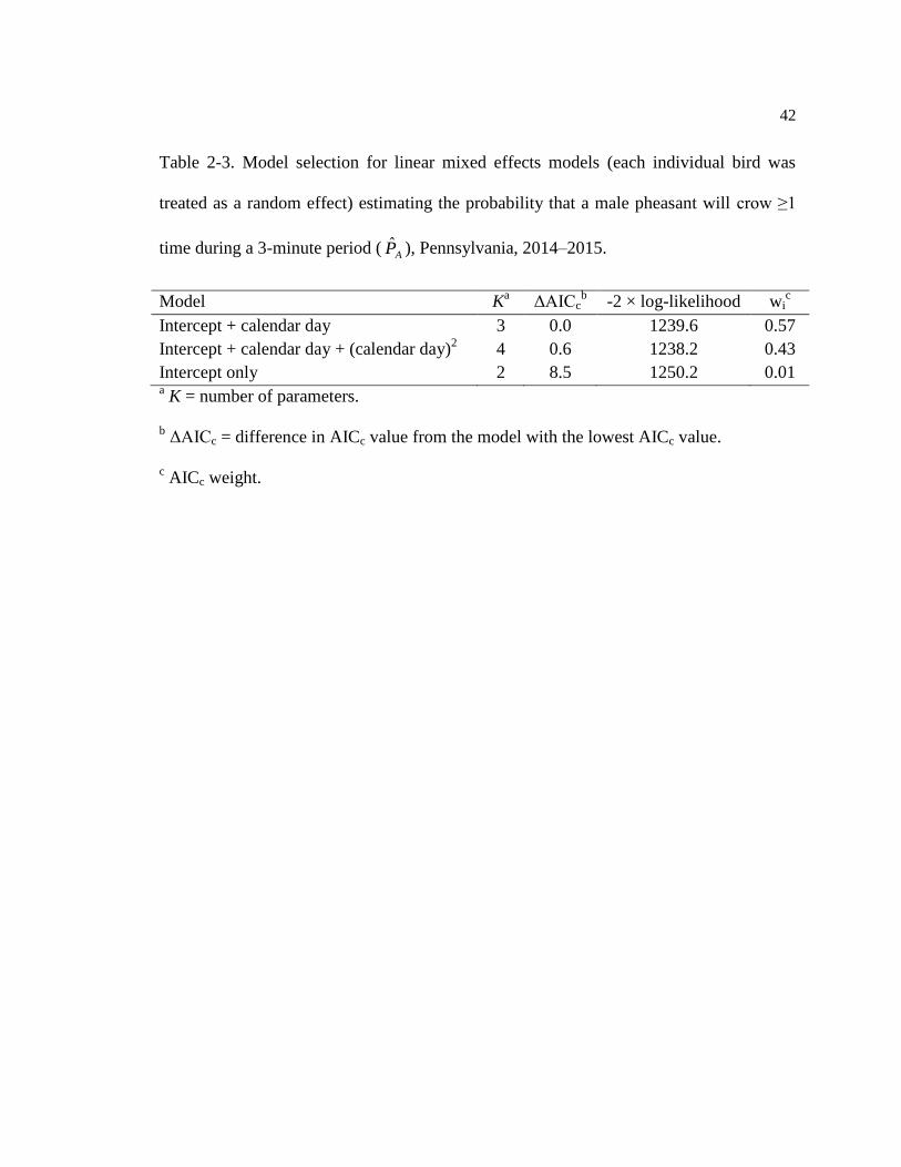
Table 2-3. Model selection for linear mixed effects models (each individual bird was

treated as a random effect) estimating the probability that a male pheasant will crow ≥1

time during a 3-minute period (AP ), Pennsylvania, 2014–2015.

Model Ka ΔAICc

b -2 × log-likelihood wi

c

Intercept + calendar day 3 0.0 1239.6 0.57

Intercept + calendar day + (calendar day)2

4 0.6 1238.2 0.43

Intercept only 2 8.5 1250.2 0.01 a K = number of parameters.

b ΔAICc = difference in AICc value from the model with the lowest AICc value.

c AICc weight.

43

Table 2-4. Model selection for the logistic regression models estimating probability that a

flushed pheasant was male. Variables in parentheses were included as random effects,

Pennsylvania, 2013–2016.

Model variables Ka Δ AICc

b -2 × log-likelihood wi

c

Intercept + (Year) 2 0.0 119.8 0.47

Intercept + Year + (WPRA) 3 0.9 117.8 0.30

Intercept + (WPRA) + (Year) 3 1.5 118.6 0.22 a K = number of parameters.

b ΔAICc = difference in AICc value from the model with the lowest AICc value.

c AICc weight.

44

Table 2-5. Density estimates (female pheasants/km2) and standard errors for female pheasants in the Somerset and Hegins-Gratz wild

pheasant recovery areas, Pennsylvania, 2013–2016.

Somerset Hegins-Gratz

North Somerset South Somerset Hegins North Gratz South Gratz

Year Density SE Density SE Density SE Density SE Density SE

2013 1.03 0.193 1.06 0.211 0.65 0.147 0.19 0.049 0.29 0.076

2014 1.05 0.230 0.66 0.145 0.55 0.117 0.31 0.074 0.21 0.052

2015 0.63 0.136 0.54 0.140 0.51 0.108 0.54 0.115 0.02 0.008

2016 0.31 0.054 0.35 0.063 0.24 0.049 0.93 0.214 0.18 0.036

45

Table 2-6. Density estimates (female pheasants/km2) and standard errors for female pheasants in the Central Susquehanna and

Franklin wild pheasant recovery areas, Pennsylvania, 2013–2016.

Central Susquehanna Franklina

Greenwood

Valley

Pennsylvania

Power and Light

Turbotville

North

Washingtonville

South

Washingtonville

West

South Franklin

Year Density SE Density SE Density SE Density SE Density SE Density SE

2013 0.96 0.189 1.32 0.262 0.84 0.168 0.56 0.112 3.75 0.787

2014 0.78 0.170 0.45 0.104 0.80 0.169 0.39 0.087 4.12 0.869 0.16 0.034

2015 0.03 0.008 1.07 0.231 1.10 0.241 0.50 0.106 4.16 0.893 0.51 0.112

2016 0.14 0.030 0.46 0.087 0.45 0.103 0.24 0.056 2.85 0.602 0.64 0.138 a The North Franklin study area had no birds detected during crowing counts in all years.

46

Figure 2-1.

47

Figure 2-2.

48

Chapter 3

Modeling potential habitat for restoration of ring-necked pheasants

Chapter 3 was written in collaboration Duane R. Diefenbach, Scott R. Klinger, and W.

David Walter. I have included this manuscript on the following pages as formatted for

The Journal of Wildlife Management.

49

ABSTRACT Ring-necked pheasant (Phasianus colchicus) are a declining game species

in much of the United States. While there has been a large amount of research concerning

habitat requirements and use of pheasants in the Midwest and western United States,

there has been less research conducted in areas with a more forest-dominated landscape.

To restore and maintain a sustainable pheasant population, knowledge of habitat

requirements in predominately forested landscapes was needed. We conducted micro-

habitat surveys (25 May–11 July) by identifying each individual habitat patch and its

vegetation characteristics within a 0.56 km radius survey circle at randomly selected sites

where we conducted crowing counts to estimate female pheasant densities. We identified

8 habitat categories a priori based on literature review and expert opinion. The

proportions of those categories within the survey circle would become the covariates in

our predictive habitat model. We found the best model for explaining female pheasant

density to include the proportion of idle grass and the proportion of forest within a survey

circle. We estimated female density to be positively influenced by the proportion of idle

grass ( = 2.612 SE = 0.344) and negatively influenced by the proportion of forest ( =

−1.050 SE = 0.317). To check the predictability of our model, we predicted densities

using the model and 2015 habitat data and found our model was useful in predicting

density but may be under-predicting compared to the actual density estimates. This model

offered insight into which habitat characteristics within appropriate pheasant habitat were

the most influential for wild pheasants during the breeding season. Using this model,

managers may be able to make more informed habitat recommendations based on the

existing habitat to meet pheasant density goals.

50

KEY WORDS habitat modeling, Pennsylvania, Phasianus colchicus, pheasant,

restoration, ring-necked pheasant

Ring-necked pheasant (Phasianus colchicus) use different habitat types depending on the

time of year, available habitat, and weather conditions. Wetlands have been found to be

crucial habitat for pheasants during the winter for thermal cover (Gates and Hale 1974,

Larsen et al. 1994, Gabbert et al. 1999), whereas grasslands are important habitat during

spring due to the vegetation they provide for nesting and rearing chicks (Schmitz and

Clark 1999). The configuration of available habitat can influence the success of nesting

pheasants more than the actual cover type or vegetation (Haensly et al. 1987, Clark and

Bogenschutz 1999, Clark et al. 1999). Leif (2005) reported male pheasants chose woody

cover and idle herbaceous habitat, but require pastures and crop fields during breeding

season to improve their chances of finding a mate.

Although pheasant are a non-native species that has been declining throughout its

range in the United States since the 1970s (Labisky 1976, Sauer et al. 2017), the

popularity of this game bird throughout the nation has resulted in a large amount of

research on habitat use in the Midwest. Much of the research focused on general habitat

selection (Gatti et al. 1989, Nielson et al. 2008), survival as influenced by habitat type

(Gabbert et al. 1999, Schmitz and Clark 1999, Homan et al. 2000), and reproductive

success due to site selection (Clark and Bogenschutz 1999, Clark et al. 1999, Matthews et

al. 2012). These studies were done in the Midwest or western part of the country (e.g.,

Iowa, Minnesota, Nebraska) in study areas with low proportions of wooded habitat

(<10%) compared to states in the eastern U.S. Although Pennsylvania was ranked second

51

for the harvest of male pheasants in 1975 (Labisky 1976), there has been less research on

the pheasant population in comparison to the Midwest states and it was not included in a

study estimating pheasant response to habitat across multiple states (Nielson et al. 2008).

In 1971, the reported average winter density ranged from 15.4 to 30.9 female

pheasants/km2 in pheasant habitat in Pennsylvania (Hartman and Sheffer 1971) but in

1993 pheasant densities ranged from 0.0 to 1.47 birds/km2 (Hardisky 1993). Pheasant

decline has been partially attributed to a loss of habitat and diversity (Taylor et al. 1978,

Warner 1984). Changes in farming practices, such as converting prime nesting habitat

into crops or using insecticides and herbicides, could decrease survival by reducing cover

and reducing the amount of food available (Warner 1984, Dahlgren 1988, Etter et al.

1988). Along with farming practices reducing the amount of habitat available to pheasant,

farming operations directly caused nest losses and led to an average mortality of 35% for

females (Hartman and Sheffer 1971). Hartman and Sheffer (1971) studied pheasant

populations in York (94.1% agricultural and 3.7% forest) and Lebanon (83.9%

agricultural and 3.9% forest) Counties that are within the 21,448 km2 of Pennsylvania

considered to be pheasant habitat. A recent study in these counties reported having a

lower proportion of agriculture (65%) and a higher proportion of forest (22%; Pabian et

al. 2015). This demonstrates how the Pennsylvania landscape has changed with an

increase in the proportion of forest and a decrease in the proportion of agriculture since

pheasant populations started to decline.

Habitat established by the Conservation Reserve Program has had a positive

influence on pheasant abundance (Riley 1995, Haroldson et al. 2006, Nielson et al. 2008).

52

The Conservation Reserve Enhancement Program (CREP) uses both state and federal

funding that is a subset of the federal Conservation Reserve Program with both programs

focusing on conversion of private land from agricultural production into conservation

practices to improve water quality habitat. These government funded programs help to

provide important potential habitat for grassland birds and other wildlife by ensuring that

there will be adequate security and thermal cover, while also providing adequate brood-

rearing habitat with grasslands. The CREP habitat of warm- and cool-season grasses had

a positive influence on pheasant populations but the estimated amount of CREP habitat

needed to prevent declines would not be attainable in Pennsylvania (Pabian et al. 2015).

Although Pabian et al. (2015) provides information about habitat currently available for

pheasants, the study only focuses on the relationship between CREP habitat and

pheasants documented at roadside counts but does not provide insight into habitat types

used by pheasants.

In an effort to restore a self-sustaining and huntable population of pheasant in

Pennsylvania, the Pennsylvania Game Commission translocated wild-trapped pheasants

from South Dakota and Montana to designated wild pheasant recovery areas (WPRAs).

To gain an understanding of the habitats the translocated pheasants were using, a habitat

use analysis on the micro-habitat level was necessary. Our objective was to assess the

habitat available on the WPRAs and create a model to predict female pheasant density

based on habitat characteristics. We expected greater pheasant densities in areas that had

high proportions of agriculture and less-intensively used habitat (e.g., warm- and cool-

season grasslands). In areas with higher proportions of forest, we expected to find lower

53

pheasant densities. With this predictive model, we can evaluate what landscape

characteristics are required to achieve a self-sustaining population to improve existing

habitat conditions on the WPRAs, as well as identify other locations in Pennsylvania

where it may be possible to restore wild pheasant populations.

STUDY AREA

Our study area included WPRAs in Pennsylvania that had >40.5 km2 of potentially

suitable breeding and overwintering habitat for pheasants. We monitored pheasant

populations in 2–5 study areas within each of the 4 WPRAs: 1) Central Susquehanna

WPRA was primarily agriculture (54.4%) with forest (16.0%) and developed land

(10.6%) (USDA National Agricultural Statistics Service Cropland Data Layer 2015)

composing the remaining habitats, 2) Somerset WPRA had a similar landscape

composition with 61.5% agriculture, 14.1% forested, and 10.7% developed, 3) Hegins-

Gratz WPRA was 63.8% agriculture, 19.6% forested, and had low development (8.8%),

and 4) Franklin WPRA was 63.5% agriculture, 13.5% forest, and 12.8% developed land.

The Central Susquehanna WPRA had the highest percentage of land enrolled in

CREP (7.1%), while the Hegins-Gratz (3.7%), Somerset (0.9%), and Franklin (0.9%)

WPRAs had lower percentages (Farm Service Agency, Washington, D.C., USA). The

Somerset WPRA had the largest percentage of wetland and shrub habitat (10.1%),

followed by Central Susquehanna WPRA (7.0%), Franklin WPRA (3.7%), and Hegins-

Gratz WPRA (1.6%; Table 3-1). The topography of the WPRAs was ridges and valleys

ranging in elevation from 106 m to 818 m (U.S. Geological Survey's Center for Earth

54

Resources Observation and Science 2010). The median frost-free growing days on the

WPRAs were 143 at Somerset, 178 at Central Susquehanna, 183 at Hegins-Gratz, and

193 at the Franklin WPRA (National Oceanic and Atmospheric Administration [NOAA]

2017a). The average yearly precipitation for the WPRAs ranged from 104 cm to 117 cm

(National Oceanic and Atmospheric Administration [NOAA] 2017b).

METHODS

Pheasant densities

We estimated female pheasant densities (pheasants/km2) at each survey circle to be the

dependent variable in the habitat model for predicting female pheasant density (Chapter

2). Because we conducted habitat surveys after the breeding season, pheasant density

estimates for the 2014 breeding season were paired with the habitat data from 2013, 2015

density estimates with 2014 habitat data, and 2016 density estimates with 2015 habitat

data.

Habitat variables

We randomly selected survey points for each study area and then moved the independent

point to the nearest road. We conducted habitat surveys at these survey points on study

areas between 25 May and 11 July, 2013–2015. We collected habitat data within a 0.56

km radius of the survey point (hereafter referred to as survey circle) because 96.9% of

birds that observers detected were within 0.56 km of the observer. At this distance, we

assumed that if observers detected a bird, then it would be using the habitat within that

55

0.56 km radius. We used digital aerial photographs from the National Agriculture

Imagery Program (USDA 2011) as the baseline imagery to delineate habitat patches. To

accurately assess the available habitat, it was necessary to evaluate the habitat annually

on a micro-habitat level instead of using aerial imagery. While aerial imagery can be

useful for identifying where different habitat types meet and the size of habitat patches, it

can be difficult to accurately delineate the actual habitat present and update changes on

an annual basis. We defined a habitat patch as an area that differed from the surrounding

area in both vegetation and appearance and this was done within each survey circle. To

create a layer of habitat at a micro-habitat scale, we assigned all patches a habitat code

according to Anderson-level land use and habitat types (Anderson 1976). We digitized

the habitat data using ArcGIS® 10.2.2 software (Environmental Systems Research

Institute, Redlands, CA, USA).

We documented 37 different micro-habitat types on 386 survey circles across all

WPRAs and years. Due to the high number of habitat types in our survey circles, we

combined habitat types by land use and biology of pheasants from a literature review and

consultations with pheasant biologists. We selected 8 habitat categories a priori to

condense our 37 possible habitat types that included (Figure 3-1): 1) developed –

developed and barren areas, 2) crop – corn, soybeans, row crops, and grains, 3) hay –

alfalfa and cool season grass fields used for hay production, 4) pasture – fenced in

grasses used for grazing, 5) idle grass – unmanaged cool and warm season grasses,

switchgrass monocultures, old fields, and herbaceous buffers, 6) shrub – areas with more

than half of the habitat in shrubs <8 m in height, orchards, and hedgerows, 7) wetlands –

56

forested, emergent, and shrub areas that were saturated with water and able to support

hydrophytes, and 8) forest – areas dominated by deciduous and mixed pine/hardwood

trees. We used the proportion of each habitat within the survey circle, the proportion of

land enrolled in CREP, and the distance of the centroid of the survey circle to the nearest

release of wild pheasants as covariates in the predictive model.

Statistical Analysis

To create a predictive model for female pheasant densities based on habitat type, we used

2 years of micro-habitat data (2013 and 2014) and density estimates (2014 and 2015).

Due to some of our estimated densities having a value of zero, we added one to the

response variable prior to performing a log transformation. We used generalized linear

mixed-effects models with a Gaussian distribution (Bates et al. 2015) to model female

pheasant densities based on habitat variables. To account for differences in land use and

repeat visits over years, we included study area and the survey circle identification as

random effects. We considered 20 candidate models a priori (Table 3-2). We used

Akaike’s Information Criterion adjusted for sample size (AICc) to select the best

approximating model and the model weight (wi) to assess the likelihood of the best model

given our data (Burnham and Anderson 2002).

To evaluate the predictive ability of the model, we used the parameter estimates

and the 2015 habitat data to predict female pheasant densities for comparison against our

estimated 2016 female pheasant densities. We used simple linear regression with the

predicted densities (calculated using the best model and habitat covariates) as the

57

independent variable and the estimated 2016 densities (estimated using the crowing count

data) as the dependent variable. We used the adjusted R2 value and the parameter

estimates to assess the predictive ability of the model. We used Pearson’s correlation

coefficient to assess how well the estimated and predicted pheasant densities agreed. We

conducted all spatial analysis, statistical tests, and model fit using R statistical

programming language (R Core Team 2015).

RESULTS

We collected habitat data on 3 WPRAs at 110 survey circles in 2013 and had 6,270

different habitat patches. In 2014, we had 4 WPRAs with 176 survey circles and 10,215

different habitat patches. For both years, the habitat type with the most patches was corn

(1,286 patches in 2013 and 1,654 patches in 2014) followed by developed land (925

patches in 2013 and 1,448 patches in 2014) and soybean (655 patches is 2013 and 946

patches in 2014). Corn was the dominant habitat type when looking at the total area

within survey circles with 29.2 km2 in 2013 and 32.3 km

2 in 2014.

Despite having relatively few patches (555 in 2013 and 812 in 2014), deciduous

forest was the second most dominant habitat type by area with a total of 22.7 km2 in 2013

and 28.3 km2 in 2014. We documented CREP on 55 of 110 survey circles in 2013 and 84

of 176 survey circles in 2014. The maximum number of habitat patches in one survey

circle in 2013 was 113 and the minimum was 23. In 2014, the maximum number of

habitat patches at one survey circle was 105 and the minimum was 15. Crop was present

58

at 99.1% of the survey circles in 2013 and 98.3% in 2014. Forest was present at 94.5% of

survey circles in 2013 and 96.0% in 2014.

The best model for predicting female pheasant density (wi = 0.84) included the

intercept ( = 0.393 SE = 0.113), the proportion of idle grass ( = 2.612 SE = 0.344),

and the proportion of forest ( = −1.050 SE = 0.317). Idle grass had a positive influence

and forest had a negative influence on female pheasant densities. The mean proportion of

forest (16.7%) and idle grasses (6.8%) observed across all survey circles predicted a

female pheasant density of 0.485 pheasants/km2. We would expect an estimated average

2.6% increase in female pheasant density with a 1% increase in the proportion of idle

grasses within the survey circle. Conversely, we estimated a 1% decrease in female

pheasant density with a 1% increase in the proportion of forest within the survey circle.

The covariates for the distance to release site and the proportions of crop, hay, pasture,

wetland, developed, shrub, or CREP were not useful in predicting female pheasant

density (Table 3-2). Crop was moderately correlated (|r| = 0.236–0.438) with the

categories of developed, pasture, idle grasses, shrub, forest, and CREP.

For 2015, we collected habitat data on 4 WPRAs with 100 survey circles to

evaluate the predictive ability of our models. The estimated slope of the regression

between predicted and actual densities was 1.609 (SE = 0.249; n = 97, r = 0.548; Figure

3-2), which indicated that the model under-predicted actual density estimates.

59

DISCUSSION

Although pheasants have been reported to use multiple habitat types throughout the year

(Hartman and Sheffer 1971, Hill and Robertson 1988, Smith et al. 1999), we found idle

grass and forest to be the best predictors of pheasant densities on our study areas.

Pheasants are considered to be an agriculturally dependent species, but we did not find

crop to be useful in predicting female pheasant densities. In our models that included

crop, the sign of the estimated parameter changed depending on the model. This

switching of the parameter sign is expected when variables are correlated, and crop was

negatively correlated with forest ( r = −0.438) and idle grass ( r = −0.367). However,

crop was present at 99.1% of survey circles in 2013 and 98.3% in 2014.

The context in which the model was created and can be applied must be

considered when using this model to identify potential pheasant restoration areas and

making informed management decisions. The boundaries of the WPRAs had a relatively

small proportion of forest, but the WPRAs were located in a landscape of about 60%

forest. Given that WPRAs were selected to be areas where predominant land use was

agriculture (>50%), our model is applicable only to areas with large proportions of

cropland. Therefore, an assumption of our model is that it is most applicable in

landscapes that are similar to land use characteristics of the WPRAs.

We conducted crowing surveys for the density estimates during the breeding

season, which provides insights into what habitat pheasants are using during this time.

Studies in Iowa, Ohio, and South Dakota found that grass was important for pheasant

60

reproduction during the breeding season and our results are consistent with these findings

(Schmitz and Clark 1999, Leif 2005, Shipley and Scott 2006). Because our density

estimates were obtained during the breeding season, our model reflects the distribution of

pheasants only during the breeding season and not at other times of the year. This may

explain why we did not find wetlands and shrubs to be useful in predicting pheasant

density. Previous research indicates that wetlands and shrub provide important habitat

and cover for pheasants during the winter (Gatti et al. 1989, Gabbert et al. 1999, Homan

et al. 2000). Smith et al. (1999) reported that shrubs and wetlands were the habitat types

used most often during the nesting season, whereas our model suggests that pheasants are

not using these habitats during the breeding season.

The proportion of forests in our WPRAs averaged 10.6–19.6%, which was

comparable to or greater than studies in the Midwest (Gatti et al. 1989, Perkins et al.

1997, Schmitz and Clark 1999). However, the fact that Pennsylvania is predominantly

forested complicates the objectives of having a sustainable, wild pheasant population

because we found the proportion of forest had a negative influence on female pheasant

densities. Given the amount of forest in Pennsylvania, it would be impossible to create

sustainable, wild pheasant populations in many areas of the state.

Federal programs, such as the Conservation Reserve Program, have a positive

effect on pheasants by creating critical habitat (Nielson et al. 2008, Matthews et al. 2012,

Pabian et al. 2015). In our study, the proportions of idle grass and CREP were highly

correlated ( r = 0.751) and therefore we did not include both in the same model.

Although CREP had a positive influence on pheasant densities, it was not included in the

61

top model and was not a better predictor of female pheasant densities than idle grass. A

large proportion of habitat we identified as idle grass was land enrolled in CREP (57.6%

in 2013 and 40.5% in 2014).

Overall, our model predicted densities that were lower than the estimated

pheasant densities, which may lead to more conservative predicted densities. This may be

due partly to the large amount of survey circles in which no birds were detected leading

to a density estimate of 0 pheasants/km2. At survey circles used to create the habitat

model, 36.0% did not have any birds detected.

MANAGEMENT IMPLICATIONS

Our predictive model can be used to make habitat improvements in attempts to meet

desired goals for pheasant densities. In landscapes similar to WPRAs in Pennsylvania

(>50% agriculture, <20% forest, <10% developed, and >20% hay), our model can

identify the percentage of land needed to be converted to idle grasses to meet pheasant

density goals, either through voluntary efforts of landowners or government-funded

programs such as CREP. However, our model does not address habitats requirements for

pheasants in Pennsylvania at other times of the year, which could be critical to population

viability.

ACKNOWLEDGMENTS

Support for this research was provided by the Pennsylvania Game Commission. We

thank volunteers who assisted with monitoring efforts and all landowners who have

62

participated in the project by maintaining pheasant habitat and allowing permission for

the access and research on their property. We would also like to thank all Pheasants

Forever and Pennsylvania Game Commission staff who assisted with the project over the

years.

LITERATURE CITED

Anderson, J. R. 1976. A land use and land cover classification system for use with remote

sensor data. Volume 964.US Government Printing Office.

Bates, D., M. Maechler, B. Bolker, and S. Walker. 2015. Fitting linear mixed-effects

models using lme4. . Journal of Statistical Software 67:1-48.

Burnham, K., and D. Anderson. 2002. Model selection and multimodel inference: a

practical information-theoretic approach. 2nd edition. Springer, New York.

Clark, W. R., and T. R. Bogenschutz. 1999. Grassland habitat and reproductive success

of ring-necked pheasants in northern Iowa Journal of Field Ornithology 70:380-

392.

Clark, W. R., R. A. Schmitz, and T. R. Bogenschutz. 1999. Site selection and nest

success of ring-necked pheasants as a function of location in Iowa landscapes.


Dahlgren, R. B. 1988. Distribution and abundance of the ring-necked pheasant in North

America. Pheasants: symptoms of wildlife problems on agricultural lands. North

Central Section of The Wildlife Society, Bloomington, Indiana, USA:29-43.

63

Etter, S. L., R. E. Warner, G. B. Joselyn, and J. E. Warnock. 1988. The dynamics of

pheasant abundance during the transition to intensive rowcropping in Illinois.

Pheasants: symptoms of wildlife problems on agricultural lands. North Central

Section of The Wildlife Society, Bloomington, Indiana, USA:111-127.

Gabbert, A. E., A. P. Leif, J. R. Purvis, and L. D. Flake. 1999. Survival and habitat use by

ring-necked pheasants during two disparate winters in South Dakota. The Journal

of Wildlife Management 63:711-722.

Gates, J. M., and J. B. Hale. 1974. Seasonal movement, winter habitat use, and

population distribution of an east central Wisconsin pheasant population.

Department of Natural Resources.

Gatti, R. C., R. T. Dumke, and C. M. Pils. 1989. Habitat use and movements of female

ring-necked pheasants during fall and winter. The Journal of Wildlife


Haensly, T. F., J. A. Crawford, and S. M. Meyers. 1987. Relationships of habitat

structure to nest success of ring-necked pheasants. The Journal of Wildlife


Hardisky, T. S. 1993. Experimental pheasant restoration program. Annual Job Report

43009. Pennsylvania Game Commission, Harrisburg, Pennsylvania, USA. .

Haroldson, K. J., R. O. Kimmel, M. R. Riggs, and A. H. Berner. 2006. Association of

ring-necked pheasant, gray partridge, and meadowlark abundance to conservation

reserve program grasslands. Journal of Wildlife Management 70:1276-1284.

64

Hartman, F., and D. Sheffer. 1971. Population dynamics and hunter harvest of ringnecked

pheasant populations in Pennsylvania’s primary range. Northeast Section of the


Hill, D., and P. Robertson. 1988. Breeding success of wild and hand-reared ring-necked

pheasants. The Journal of Wildlife Management:446-450.

Homan, H. J., G. M. Linz, and W. J. Bleier. 2000. Winter habitat use and survival of

female ring-necked pheasants (Phasianus colchicus) in southeastern North

Dakota. The American midland naturalist 143:463-480.

Labisky, R. F. 1976. Midwest pheasant abundance declines. Wildlife Society Bulletin

(1973-2006) 4:182-183.

Larsen, D. T., P. L. Crookston, and L. D. Flake. 1994. Factors associated with ring-

necked pheasant use of winter food plots. Wildlife Society Bulletin 22:620-626.

Leif, A. P. 2005. Spatial ecology and habitat selection of breeding male pheasants.

Wildlife Society Bulletin 33:130-141.

Matthews, T. W., J. S. Taylor, and L. A. Powell. 2012. Ring‐necked pheasant hens select

managed Conservation Reserve Program grasslands for nesting and brood‐

rearing. The Journal of Wildlife Management 76:1653-1660.

National Oceanic and Atmospheric Administration [NOAA]. 2017a. National Weather

Service internet services team. Normal Dates of Last Freeze in Spring and First

Freeze in Autumn. <https://www.weather.gov/ctp/FrostFreeze>. Accessed 6 June

2017.

https://www.weather.gov/ctp/FrostFreeze%3e

65

National Oceanic and Atmospheric Administration [NOAA]. 2017b. National Weather

Service internet services team. Pennsylvania 30 Year (1971-2000) Mean Annual

Precipitation. <http://www.weather.gov/ctp/moreHydro>. Accessed 6 June 2017.








Perkins, A. L., W. R. Clark, T. Z. Riley, and P. A. Vohs. 1997. Effects of landscape and

weather on winter survival of ring-necked pheasant hens. The Journal of Wildlife


R Core Team. 2015. R : A language and environment for statistical computing. R

Foundation for Statistical Computing. Vienna, Austria. https://www.R-

project.org/.

Riley, T. Z. 1995. Association of the conservation reserve program with ring-necked

pheasant survey counts in Iowa. Wildlife Society Bulletin (1973-2006) 23:386-

390.

Sauer, J. R., D. K. Niven, J. E. Hines, D. J. Ziolkowski Jr, K. L. Pardieck, J. E. Fallon,

and W. A. Link. 2017. The North American breeding bird survey, results and

analysis 1996-2015. Version 2.07.2017. USGS Patuxent Wildlife Research

Center, Laurel, MD.

http://www.weather.gov/ctp/moreHydro%3e



66

Schmitz, R. A., and W. R. Clark. 1999. Survival of ring-necked pheasant hens during

spring in relation to landscape features. The Journal of Wildlife Management

63:147-154.

Shipley, K. L., and D. P. Scott. 2006. Survival and nesting habitat use by sichuan and

ring-necked pheasants released in Ohio. The Ohio Journal of Science 106:78.

Smith, S. A., N. J. Stewart, and J. E. Gates. 1999. Home ranges, habitat selection and

mortality of ring-necked pheasants (Phasianus colchicus) in North-central

Maryland. The American midland naturalist 141:185-197.

Taylor, M. W., C. W. Wolfe, and W. L. Baxter. 1978. Land-use change and ring-necked

pheasants in Nebraska. Wildlife Society Bulletin:226-230.

U.S. Geological Survey's Center for Earth Resources Observation and Science. 2010. 30

arc-second DEM of North America [Online]. Available at


4.

USDA. 2011. USDA geospatial data gateway. <http://datagateway.nrcs.usda.gov/>.

Accessed 15 May 2017.

USDA National Agricultural Statistics Service Cropland Data Layer. 2015. Published

crop-specific data layer [Online]. Available at

https://nassgeodata.gmu.edu/CropScape/ (accessed 2/21/16; verified 2/12/16).

USDA-NASS, Washington, DC.

Warner, R. E. 1984. Effects of changing agriculture on ring-necked pheasant brood

movements in Illinois. The Journal of Wildlife Management 48:1014-1018.



http://datagateway.nrcs.usda.gov/%3e

https://nassgeodata.gmu.edu/CropScape/

67

Figure 3-1. An example of a survey circle (0.56 km radius) with the different habitat

patches categorized according to the Anderson-level land use (A; Anderson 1976) and the

same survey circle combined using our 8 habitat categories (B).

Figure 3-2. The predicted female pheasant density (female pheasants/km2) plotted against

the estimated female pheasant density (female pheasants/km2) with the line of best fit

(solid) and a one-to-one ratio (dashed).

68

Table 3-1. Survey circles, size of wild pheasant recovery areas (WPRAs) and study areas, and the average proportion of habitat per

survey circle (%). The Conservation Reserve Enhancement Program (CREP; Farm Service Agency, Washington, D.C., USA) habitat

proportions were calculated separately and may overlap other categories, Pennsylvania, 2013–2015.

WPRA

Study area

Number of survey

circles

Area

(km2)

Develop Crop Hay Pasture

Idle

grass Shrub Wetlands Forest CREP 2013 2014 2015

Central Susquehanna 55 97 47 511.6

Greenwood Valley 10 19 9 66.0 11.6 26.8 8.9 7.2 10.7 9.1 2.4 20.8 8.5

Pennsylvania Power & Light 10 16 10 80.9 7.3 35.9 10.1 7.8 9.2 7.1 1.0 18.3 7.6

Turbotville North 11 22 10 78.9 13.9 39.8 7.6 4.5 9.4 6.6 0.5 16.5 4.7

Washingtonville South 5 20 6 90.9 8.8 37.9 9.2 4.0 8.0 5.9 0.5 19.6 7.3

Washingtonville West 19 20 12 80.2 9.5 53.3 10.0 6.4 9.3 3.4 0.1 6.9 7.9

Hegins-Gratz 32 45 23 255.8

Hegins 12 16 9 62.2 10.3 39.1 9.3 1.8 9.5 2.2 0.1 26.4 6.7

North Gratz 10 15 7 40.5 8.6 55.0 12.0 5.4 2.2 1.5 0.1 14.2 0.6

South Gratz 10 14 7 42.1 7.5 47.2 17.4 7.0 2.8 0.7 0.0 16.1 2.8

Somerset 23 21 16 69.2

North Somerset 15 14 12 51.3 10.9 33.8 26.6 4.1 2.2 0.9 6.7 13.6 0.7

South Somerset 8 7 4 17.8 10.5 25.7 24.0 4.3 6.2 7.3 6.4 14.8 1.0

Franklin 0 13 14 339.9

South Franklin 0 13 14 55.7 12.4 35.1 18.7 9.8 5.8 3.3 0.1 13.1 0.4

69

Table 3-2. Parameters, number of parameters (K), difference in value from the model 1

with the model having the lowest AICc value (Δ AICc), -2 × log-likelihood, and weights 2

(wi) for linear mixed effects models estimating female pheasant density (log(Female 3

Density+1) based on micro-habitat variables in Pennsylvania, 2013–2015. Study area and 4

circle identification were included in all models as random effects. 5

6

Parameters

K

Δ AICc

-2 × log-likelihood wi

Idle Grass+Forest 6 0.0 435.6 0.84

Idle Grass+Forest+Distance+ Distance2 8 4.57 436.0 0.09

Crop+Idle Grass+Forest+Distance+Distance2

9 6.29 435.5 0.04

Idle Grass 5 7.81 445.5 0.02

Crop+Idle Grass+Distance+Distance2 8 8.13 439.5 0.01

Idle Grass+Distance+Distance2 7 9.89 443.4 0.01

CREP+Forest 6 18.16 453.8 0.00

Crop+CREP+Forest 7 20.89 454.4 0.00

CREP+Forest+Distance+Distance2

8 21.13 452.5 0.00

CREP 5 21.88 459.6 0.00

Crop+CREP+Forest+Distance+Distance2 9 24.10 453.4 0.00

Forest+Distance+Distance2 7 38.61 472.1 0.00

Distance+Distance2 6 41.67 477.3 0.00

Developed 5 41.88 479.6 0.00

Forest 5 46.46 484.2 0.00

Wetland 5 49.32 487.0 0.00

Shrub 5 49.77 487.5 0.00

Pasture 5 52.93 490.6 0.00

Hay 5 52.98 490.7 0.00

Crop 5 54.75 492.4 0.00

70

Figure 3-1.

71

Figure 3-2.

72

Chapter 4

The future of ring-necked pheasants in Pennsylvania

73

Overall, the reintroduction of wild pheasants to Pennsylvania was not successful because

most study areas (11 of 12) did not reach the pheasant density goal of 3.86 females/km2.

At the only successful study area (Washingtonville West), the expected density

(assuming no births, deaths, or movement since release of wild pheasants) based solely

on the number of released birds was 2.13 female pheasants/km2 with the last pheasant

release on this study area in 2009. Because we estimated the female density in 2013–

2016 to exceed the released density, it appears that reproduction is naturally occurring on

the study area and the population is increasing.

Insight into why the Washingtonville West study area had a successful

reintroduction can be gained from reviewing the habitat modeling results from Chapter 3.

Washingtonville West had the lowest proportion of forest in the survey circles among all

study areas, ranging from 4.3% to 9.3% across study years. The average proportion of

idle grass in the survey circles from 2013 to 2015 was greater (7.9–10.8%) than some of

the other study areas. At the average proportion of forest (6.5%), the model predicted that

an average of 14.0% of the habitat in survey circles would need to be idle grass to

achieve the density goal. The average proportion of idle grass in survey circles (9.1%) on

Washingtonville West in 2015 was similar to what the model predicted (13.0%). Even

with the low forest density that is present at Washingtonville West, the predicted

proportion of idle grass needed to support the goal density of pheasants is barely

sufficient and the amount of idle grass habitat on all study areas is likely the most

challenging issue for pheasant population restoration.

No other study areas came close to meeting the expected habitat requirements

necessary to reach the density goal and none exceeded a density of 2 female

74

pheasants/km2. Over all the study areas (including Washingtonville West), the average

proportion of forest in survey circles was 16.5% and based on that, the model predicted

an average of 18.0% idle grass to meet female pheasant density goals but the average

proportion of idle grass in survey circles across all study areas was 7.0%. I believe the

lack of idle grass in relation to the amount of forest that was present in these areas helped

explain why almost all of the study areas failed to achieve density goals.

Pennsylvania is 65.8% forested (Nowak and Greenfield 2012) which limits the

amount of landscape suitable for wild, sustainable pheasant populations due to the

negative effect our study found forest to have on pheasant densities. When applying the

model to other areas of Pennsylvania, the context in which the model was created is

important. The model estimated the most influential habitat characteristics in a landscape

that was first identified as being suitable for pheasants by meeting the WPRA criteria

(<20% forested, >50% agriculture, <10% developed, and >20% hay). Model results

indicated that in landscapes that achieved WPRA criteria, idle grass and forest were the

habitat characteristics most influencing pheasant densities. When attempting to identify

potential pheasant habitat, areas that meet or exceed WPRA habitat ideally would be

prioritized. In these areas, randomly selected sites (as described in Chapter 3) could be

used to evaluate habitat conditions. Wildlife managers could then use the habitat model to

determine what improvements would be necessary to achieve the habitat needed for

desired pheasant density goals. For example, areas with a low proportion of forest are

given priority because they are expected to require less idle grass to support pheasants.

Also, managers could then identify the amount of idle grass that needed to be created, via

personal interest or government assistance programs. Although the Conservation Reserve

75

Enhancement Program (CREP) did provide idle grass habitat, it was not as good a

predictor for pheasant densities as idle grass. Currently, there does not appear to be

enough CREP or idle grass habitat to support sustainable pheasant densities in most

places of the state. CREP does seem helpful in ensuring there is grassland habitat in

Pennsylvania, but it does not appear to provide enough habitat to reverse pheasant

declines (Pabian et al. 2015).

Due to the negative effect of forest on pheasant densities, it is probably unrealistic

that Pennsylvania will be able to reach pheasant density estimates similar to the peaks in

the 1960s and 1970s that many pheasant hunters experienced. This study does not

examine the underlying cause of the pheasant decline or how it could be reversed, but it

does offer important insight into future management for this iconic species in the

Pennsylvania landscape. With proper management, regulation, and monitoring it is

possible to maintain wild populations of pheasants in some areas of the state, although it

is unlikely these small populations will be able to sustainably provide hunting

opportunities to all of Pennsylvania’s hunters. Based on Pennsylvania’s current

landscapes and land use, it is unlikely a sustainable wild pheasant population could be

established statewide.

LITERATURE CITED

Nowak, D. J., and E. J. Greenfield. 2012. Tree and impervious cover in the United States.

Landscape and Urban Planning 107:21-30.

76




The Pennsylvania State University - Amazon Web … Pennsylvania State University The Graduate School...

Documents

Transcript of The Pennsylvania State University - Amazon Web … Pennsylvania State University The Graduate School...