The partition function of the two-matrix model as an - HAL

HAL Id: hal-00863565https://hal.archives-ouvertes.fr/hal-00863565

Submitted on 19 Sep 2013

HAL is a multi-disciplinary open accessarchive for the deposit and dissemination of sci-entific research documents, whether they are pub-lished or not. The documents may come fromteaching and research institutions in France orabroad, or from public or private research centers.

L’archive ouverte pluridisciplinaire HAL, estdestinée au dépôt et à la diffusion de documentsscientifiques de niveau recherche, publiés ou non,émanant des établissements d’enseignement et derecherche français ou étrangers, des laboratoirespublics ou privés.

The partition function of the two-matrix model as anisomonodromic tau-function

Bertola Marco, Olivier Marchal

To cite this version:Bertola Marco, Olivier Marchal. The partition function of the two-matrix model as an isomon-odromic tau-function. Journal of Mathematical Physics, American Institute of Physics (AIP), 2009,50, pp.013529. <10.1063/1.3054865>. <hal-00863565>

https://hal.archives-ouvertes.fr/hal-00863565

https://hal.archives-ouvertes.fr

The partition function of the two-matrix model as anisomonodromic � function

M. Bertola3,2,a� and O. Marchal1,2,b�

1Institut de Physique Théorique, CEA, IPhT, F-91191 Gif-sur-Yvette, France and CNRS,

URA 2306, F-91191 Gif-sur-Yvette, France2Centre de Recherches Mathématiques, Université de Montréal, C. P. 6128, succ. centre

ville, Montréal, Québec H3C 3J7, Canada3Department of Mathematics and Statistics, Concordia University, 1455 de Maisonneuve

W., Montréal, Québec H3G 1M8, Canada

�Received 9 September 2008; accepted 1 December 2008; published online 15 January 2009�

We consider the Itzykson–Zuber–Eynard–Mehta two-matrix model and prove that

the partition function is an isomonodromic � function in a sense that generalizes

that of Jimbo et al. � “Monodromy preserving deformation of linear ordinary dif-

ferential equations with rational coefficients,” Physica D 2, 306 �1981��. In order to

achieve the generalization we need to define a notion of � function for isomono-

dromic systems where the adregularity of the leading coefficient is not a necessary

requirement. © 2009 American Institute of Physics. �DOI: 10.1063/1.3054865�

I. INTRODUCTION

Random matrix models have been studied for years and have generated important results in

many fields of both theoretical physics and mathematics.1,16,18

The two-matrix model

d��M1,M2� = e−Tr�V1�M1�+V2�M2�−M1M2�dM1dM2 �1.1�

was used to model two-dimensional quantum gravity14

and was investigated from a more math-

ematical point of view in Refs. 25, 17, 4, 5, 7, 12, and 8; the partition function of the model

ZN�V1,V2� =� � d��M1,M2� �1.2�

has important properties in the large N limit for the enumeration of discrete maps on surfaces15

of

arbitrary genus and it is also known to be a � function for the 2-Toda hierarchy. In the case of the

Witten conjecture, proved by Kontsevich23

with the use of matrix integrals not too dissimilar from

the above one, the enumerative properties of the � function imply some nonlinear �hierarchy of�partial differential equations �PDEs� �the Korteweg-de Vries �KdV� hierarchy for the mentioned

example�. On a similar level, one expects some hierarchy of PDEs for the case of the two-matrix

model and possibly some Painlevé property �namely, the absence of movable essential singulari-

ties�. The Painlevé property is characteristic of � functions for isomonodromic families of ordinary

differential equations �ODEs� that depend on parameters; hence, a way of establishing such prop-

erty for the partition function ZN is that of identifying it with an instance of isomonodromic �function.

20,21

This is precisely the purpose of this article; we capitalize on previous work that showed how

to relate the matrix model to certain biorthogonal polynomials26,17,22,16

and how these appear in a

natural fashion as the solution of certain isomonodromic family.9

a�Electronic mail: [email protected].

b�Electronic mail: [email protected].

JOURNAL OF MATHEMATICAL PHYSICS 50, 013529 �2009�

50, 013529-10022-2488/2009/50�1�/013529/17/$25.00 © 2009 American Institute of Physics

Downloaded 22 Sep 2009 to 132.166.22.147. Redistribution subject to AIP license or copyright; see http://jmp.aip.org/jmp/copyright.jsp

http://dx.doi.org/10.1063/1.3054865

http://dx.doi.org/10.1063/1.3054865

http://dx.doi.org/10.1063/1.3054865

The paper extends to the case of the two-matrix model the work contained in Refs. 9, 12, and

10; it uses, however, a different approach closer to a recent one.6

In Refs. 9, 12, 10, and 19 the partition function of the one-matrix model �and certain shifted

Töplitz determinants� were identified as isomonodromic � functions by using spectral residue

formulas in terms of the spectral curve of the differential equation. Such spectral curve has

interesting properties inasmuch as—in the one-matrix case—the spectral invariants can be related

to the expectation values of the matrix model. Recently the spectral curve of the two-matrix

model8

has been written explicitly in terms of expectation values of the two-matrix model and

hence one could use their result and follow a similar path for the proof as the one followed in Ref.

12. Whichever one of the two approaches one chooses, a main obstacle is that the definition of

isomonodromic � function20,21

relies on a genericity assumption for the ODE which fails in the

case at hand, thus requiring a generalization in the definition �see, however, Ref. 11 for a different

generalization�.According to this logic, one of the purposes of this paper is to extend the notion of � function

introduced by Jimbo et al.20

to the two-matrix Itzykson–Zuber model. This task is accomplished in

a rather general framework in Sec. III.

We then show that the partition function has a very precise relationship with the � function so

introduced, allowing us to �essentially� identify it as an isomonodromic � function �Theorem 3.4�.The proof is organized as follows. In Sec. II we recall a Riemann–Hilbert formulation of the

problem due to Ref. 24. In Sec. II B we transform it into a Riemann-Hilbert problem �RHP� with

constant jumps, thus guaranteeing the existence of an ODE. As the asymptotic at infinity does not

enter into the class of the Jimbo–Miwa theorem for isomonodromic � function, we generalize their

result to our setting in Sec. III. Using Schlesinger transformations, namely, the shift in the size of

the matrix model from N to N+1, we eventually show that the partition function equals the new

defined isomonodromic � function in Sec. III B.

II. A RIEMANN–HILBERT FORMULATION OF THE TWO-MATRIX MODEL

According to a seminal work26,17

and following the notations and definitions introduced in

Refs. 4 and 5, we consider paired sequences of monic polynomials ��m�x� ,�m�y��m=0,. . .,� �m=deg �m=deg �m� that are biorthogonal in the sense that

� ��

dxdy�m�x��n�y�e−V1�x�−V2�y�+xy = hm�mn, hm � 0. �2.1�

The functions V1�x� and V2�y� appearing here are referred to as potentials, terminology drawn

from random matrix theory, in which such quantities play a fundamental role.

Henceforth, the second potential V2�y� will be chosen as a polynomial of degree d2+1,

V2�y� = �J=1

d2+1vJ

JyJ, vd2+1 � 0. �2.2�

For the purposes of most of the considerations to follow, the first potential V1�x� may have very

general analyticity properties as long as the manipulations make sense, but for definiteness and

clarity, we choose it to be polynomial as well:

V1�x� = �K=1

d1+1uK

KxK, ud1+1 � 0. �2.3�

The symbol � stands for any linear combination of integrals of the form

013529-2 M. Bertola and O. Marchal J. Math. Phys. 50, 013529 �2009�


� ��

dxdy ª �j

�k

� jk��j

dx��k

dy, �ij � C , �2.4�

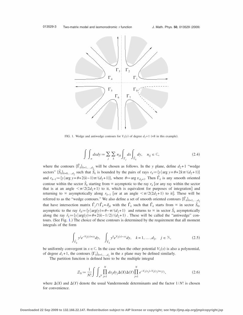
where the contours ��k�k=1,. . .,d2will be chosen as follows. In the y plane, define d2+1 “wedge

sectors” �Sk�k=0,. . .,d2such that Sk is bounded by the pairs of rays rkª �y arg y=+2k� / �d2+1��

and rk−1ª �y arg y=+2�k−1�� / �d2+1��, where ªarg vd2+1. Then �k is any smooth oriented

contour within the sector Sk starting from � asymptotic to the ray rk �or any ray within the sector

that is at an angle � /2�2d2+1� to it, which is equivalent for purposes of integration� and

returning to � asymptotically along rk−1 �or at an angle � /2�2d2+1� to it�. These will be

referred to as the “wedge contours.” We also define a set of smooth oriented contours ��k�k=1,. . .,d2

that have intersection matrix � j � �k=� jk with the �k such that �k starts from � in sector S0,

asymptotic to the ray r0ª �y arg�y�=−� / �d2+1�� and returns to � in sector Sk asymptotically

along the ray rkª �y arg�y�=+2�k−1 /2� / �d2+1��. These will be called the “antiwedge” con-

tours. �See Fig. 1.� The choice of these contours is determined by the requirement that all moment

integrals of the form

��k

y je−V2�y�+xydy, ��k

ykeV2�y�−xydy, k = 1, . . . ,d2, j � N , �2.5�

be uniformly convergent in x�C. In the case when the other potential V1�x� is also a polynomial,

of degree d1+1, the contours ��k�k=1,. . .,d1in the x plane may be defined similarly.

The partition function is defined here to be the multiple integral

ZN ª1

N!� �

�N�j=1

N

dx jdy j��X��Y��j=1

N

e−V1�xj�−V2�y j�+xjy j , �2.6�

where ��X� and ��Y� denote the usual Vandermonde determinants and the factor 1 /N! is chosen

for convenience.

ΓΓ

Γ

Γ

Γ Γ

Γ

Γ0

1

23

4

5

6 7

FIG. 1. Wedge and antiwedge contours for V2�y� of degree d2+1 �=8 in this example�.

013529-3 Two-matrix model and isomonodromic � function J. Math. Phys. 50, 013529 �2009�


Such multiple integral can also be represented as the following determinant:

ZN = det��ij�0�i,j�N−1, �ij ª ��

xiy je−V1�x�−V2�y�+xydxdy . �2.7�

The denomination of the partition function comes from the fact26,17,9

that when � coincides with

R R then ZN coincides �up to a normalization for the volume of the unitary group� with the

following matrix integral:

� � dM1dM2e−tr�V1�M1�+V2�M2�−M1M2�, �2.8�

extended over the space of Hermitian matrices M1 and M2 of size N N, namely, the normaliza-

tion factor for the measure d��M1 ,M2� introduced in �1.1�.

A. Riemann–Hilbert characterization for the orthogonal polynomials

A Riemann–Hilbert characterization of the biorthogonal polynomials is a crucial step toward

implementing a steepest-descent analysis. In our context it is also crucial in order to tie the random

matrix side to the theory of isomonodromic deformations.

We first recall the approach given by Kuijlaars and McLaughin �referred to as KM in the rest

of the article� in Ref. 24 suitably extended and adapted �in a rather trivial way� to the setting and

notation of the present work. We quote—paraphrasing and with a minor generalization—their

theorem without proof.

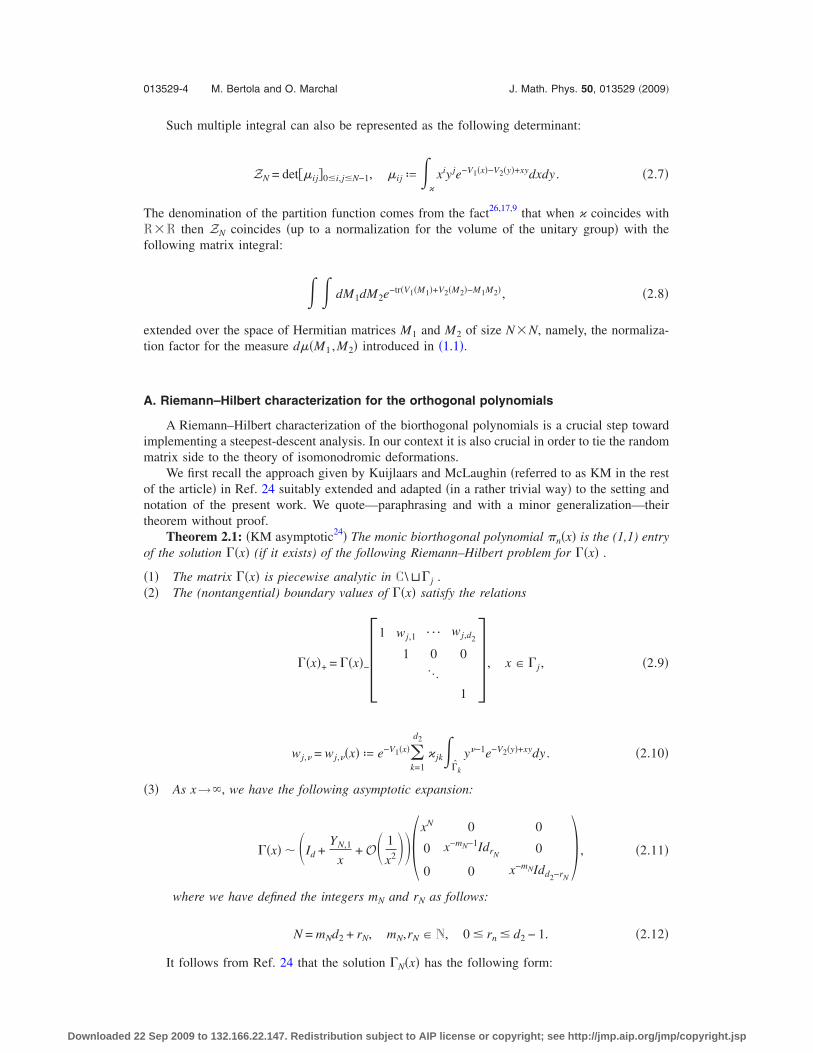
Theorem 2.1: �KM asymptotic24� The monic biorthogonal polynomial �n�x� is the (1,1) entry

of the solution ��x� (if it exists) of the following Riemann–Hilbert problem for ��x� .

�1� The matrix ��x� is piecewise analytic in C \ ⊔� j .

�2� The (nontangential) boundary values of ��x� satisfy the relations

��x�+ = ��x�−�1 w j,1 ¯ w j,d2

1 0 0

�

1 , x � � j , �2.9�

w j,� = w j,��x� ª e−V1�x��k=1

d2

� jk��k

y�−1e−V2�y�+xydy . �2.10�

�3� As x→�, we have the following asymptotic expansion:

��x� � �Id +YN,1

x+ O� 1

x2��xN 0 0

0 x−mN−1IdrN0

0 0 x−mNIdd2−rN

� , �2.11�

where we have defined the integers mN and rN as follows:

N = mNd2 + rN, mN,rN � N, 0 � rn � d2 − 1. �2.12�

It follows from Ref. 24 that the solution �N�x� has the following form:



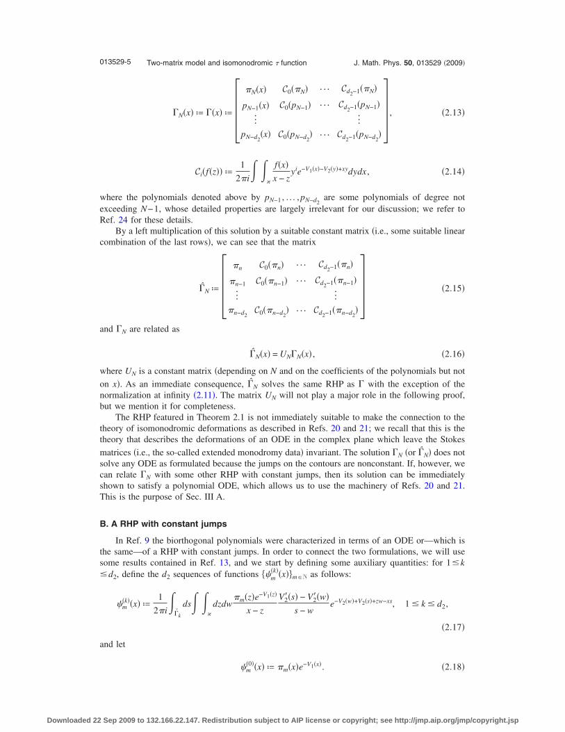
�N�x� ª ��x� ª ��N�x� C0��N� ¯ Cd2−1��N�

pN−1�x� C0�pN−1� ¯ Cd2−1�pN−1�

] ]

pN−d2�x� C0�pN−d2

� ¯ Cd2−1�pN−d2� , �2.13�

Ci�f�z�� ª1

2�i� �

�

f�x�x − z

yie−V1�x�−V2�y�+xydydx , �2.14�

where the polynomials denoted above by pN−1 , . . . , pN−d2are some polynomials of degree not

exceeding N−1, whose detailed properties are largely irrelevant for our discussion; we refer to

Ref. 24 for these details.

By a left multiplication of this solution by a suitable constant matrix �i.e., some suitable linear

combination of the last rows�, we can see that the matrix

�N ª ��n C0��n� ¯ Cd2−1��n�

�n−1 C0��n−1� ¯ Cd2−1��n−1�

] ]

�n−d2C0��n−d2

� ¯ Cd2−1��n−d2� �2.15�

and �N are related as

�N�x� = UN�N�x� , �2.16�

where UN is a constant matrix �depending on N and on the coefficients of the polynomials but not

on x�. As an immediate consequence, �N solves the same RHP as � with the exception of the

normalization at infinity �2.11�. The matrix UN will not play a major role in the following proof,

but we mention it for completeness.

The RHP featured in Theorem 2.1 is not immediately suitable to make the connection to the

theory of isomonodromic deformations as described in Refs. 20 and 21; we recall that this is the

theory that describes the deformations of an ODE in the complex plane which leave the Stokes

matrices �i.e., the so-called extended monodromy data� invariant. The solution �N �or �N� does not

solve any ODE as formulated because the jumps on the contours are nonconstant. If, however, we

can relate �N with some other RHP with constant jumps, then its solution can be immediately

shown to satisfy a polynomial ODE, which allows us to use the machinery of Refs. 20 and 21.

This is the purpose of Sec. III A.

B. A RHP with constant jumps

In Ref. 9 the biorthogonal polynomials were characterized in terms of an ODE or—which is

the same—of a RHP with constant jumps. In order to connect the two formulations, we will use

some results contained in Ref. 13, and we start by defining some auxiliary quantities: for 1�k

�d2, define the d2 sequences of functions ��m

�k��x��m�N as follows:

�m�k��x� ª

1

2�i�

�k

ds� ��

dzdw�m�z�e−V1�z�

x − z

V2��s� − V2��w�

s − we−V2�w�+V2�s�+zw−xs, 1 � k � d2,

�2.17�

and let

�m�0��x� ª �m�x�e−V1�x�. �2.18�



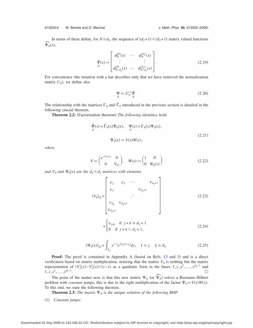
In terms of these define, for N�d2, the sequence of �d2+1� �d2+1� matrix valued functions

�N�x�,

�N

�x� ª ��N

�0��x� ¯ �N�d2��x�

] ]

�N−d2

�0� �x� ¯ �N−d2

�d2� �x� . �2.19�

For convenience �the notation with a hat describes only that we have removed the normalization

matrix UN�, we define also

�N

ª UN−1�

N. �2.20�

The relationship with the matrices �N and �N introduced in the previous section is detailed in the

following crucial theorem.

Theorem 2.2: �Factorization theorem� The following identities hold:

�N

�x� = �N�x��0�x�, �N

�x� = �N�x��0�x� ,

�2.21��0�x� ª V�x�W�x� ,

where

V ª �e−V1�x� 0

0 V0,�, W�x� ª �1 0

0 W0�x�� 2.22�

and V0 and W0�x� are the d2 d2 matrices with elements

�V0� jk = �v2 v3 ¯ vd2+1

v3 vd2+1

�

vd2vd2+1

vd2+1

�2.23�

=�v j+k if j + k � d2 + 1

0 if j + k � d2 + 1,� �2.24�

�W0�x�� jk = ��k

y j−1eV2�y�−xydy, 1 � j, k � d2. �2.25�

Proof: The proof is contained in Appendix A �based on Refs. 13 and 3� and is a direct

verification based on matrix multiplication, noticing that the matrix V0 is nothing but the matrix

representation of �V2��y�−V2��s�� / �y−s� as a quadratic form in the bases 1 ,y ,y2 , . . . ,yd2−1 and

1,s ,s2 , . . . ,sd2−1. �

The point of the matter now is that this new matrix �N �or �N� solves a Riemann–Hilbert

problem with constant jumps; this is due to the right multiplication of the factor �0ªV�x�W�x�.To this end, we state the following theorem.

Theorem 2.3: The matrix �N is the unique solution of the following RHP.

�1� Constant jumps:



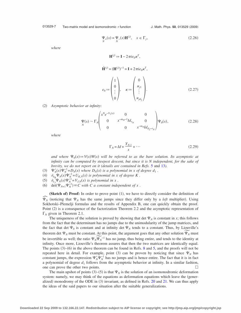
�N

+�x� = �N

−�x�H�j�, x � � j , �2.26�

where

H�j� ª I − 2�ie0�T,

H�j� = �H�j��−1 = I + 2�ie0�T,

e0 ª�1

0

]

0�, � ª�

0

� j1

]

� jd2

� . �2.27�

�2� Asymptotic behavior at infinity:

�N

�x� � �N�xNe−V1�x� 0 0

0 x−mN−1IdrN0

0 0 x−mNIdd2−rN

��0�x� , �2.28�

where

�N = Id +YN,1

x+ ¯ �2.29�

and where �0�x�ªV�x�W�x� will be referred to as the bare solution. Its asymptotic at

infinity can be computed by steepest descent, but since it is N independent, for the sake of

brevity, we do not report on it (details are contained in Refs. 5 and 13).

�3� �N� �x��N−1=DN�x� where DN�x� is a polynomial in x of degree d1 .

�4� �uK�N�x��N

−1=UK,N�x� is polynomial in x of degree K .

�5� �vJ

�N�x��N−1=VJ,N�x� is polynomial in x .

�6� det��N+1�N−1��C with C a constant independent of x .

(Sketch of) Proof: In order to prove point �1�, we have to directly consider the definition of

�N �noticing that �N has the same jumps since they differ only by a left multiplier�. Using

Sokhotski–Plemelji formulas and the results of Appendix B, one can quickly obtain the proof.

Point �2� is a consequence of the factorization Theorem 2.2 and the asymptotic representation of

�N given in Theorem 2.1.

The uniqueness of the solution is proved by showing that det �N is constant in x; this follows

from the fact that the determinant has no jumps due to the unimodularity of the jump matrices, and

the fact that det �0 is constant and at infinity det �N tends to a constant. Thus, by Liouville’s

theorem det �N must be constant. At this point, the argument goes that any other solution �N˜ must

be invertible as well; the ratio �N�N˜−1 has no jump, thus being entire, and tends to the identity at

infinity. Once more, Liouville’s theorem assures that then the two matrices are identically equal.

The points �3�–�6� in the above theorem can be found in Refs. 8 and 5, and the proofs will not be

repeated here in detail. For example, point �3� can be proven by noticing that since �N has

constant jumps, the expression �N��N−1 has no jumps and is hence entire. The fact that it is in fact

a polynomial of degree d1 follows from the asymptotic behavior at infinity. In a similar fashion,

one can prove the other two points. �

The main upshot of points �3�–�5� is that �N is the solution of an isomonodromic deformation

system: namely, we may think of the equations as deformation equations which leave the �gener-

alized� monodromy of the ODE in �3� invariant, as defined in Refs. 20 and 21. We can thus apply

the ideas of the said papers to our situation after the suitable generalizations.



In the next section, we shall define a proper notion of isomonodromic � function: it should be

pointed out that the definition of Refs. 20 and 21 cannot be applied as such because—as shown in

Ref. 5—the ODE that the matrix �N �or �N� solves has a highly degenerate leading coefficient at

the singularity at infinity.

In the list, the crucial ingredients are the differential equations �in x or relatively to the

parameters uK and vJ�. First, the fact that DN�x� is a polynomial comes from explicit computation

�see Ref. 8, for example�. The result concerning the determinant of RN�x� can also be found in Ref.

8 where one has det��N+1�N−1�=det�aN�x��=Cste. The properties concerning the differential equa-

tions relatively to parameters can be found in Ref. 8 too. Under all these assumptions, we will

show that the proof of Jimbo et al. can be adapted and that we can define a suitable � function in

the same way Jimbo et al. did.

III. DEFINITION OF THE � FUNCTION

In this section, we will place ourselves in a more general context than the one described

above; we will show that, under a few assumptions, one can define a good notion of � function.

More generally, we will denote with ta the isomonodromic parameters or “isomonodromic

times” �in our case they are the uK and the vJ� and a subscript a or b is understood as a derivation

relative to ta or tb. For a function f of the isomonodromic times, we will denote by the usual

symbol its differential,

df = �a

�tafdta = �

a

fadta. �3.1�

Our setup falls in the following framework that it is useful to ascertain from the specifics of the

case at hand. Suppose we are given a matrix whose behavior at infinity is

��x� � Y�x��x�, Y�x� ª �1 +Y1

x+

Y2

x2+ ¯�xS, �3.2�

where ��x�=��x ; t� is some explicit expression �the “bare” isomonodromic solution� and S is a

matrix independent of the isomonodromic times. Note that this asymptotic falls exactly in the one

we get for �N�x�. This implies that if we define the one-form-valued matrix H�x ; t� by

H�x;t� = d��x;t��x;t�−1 �3.3�

then H�x�=�Hadta �we suppress explicit mention of the t dependence henceforth� is some solu-

tion of the zero-curvature equations:

�aHb − �bHa = �Ha,Hb� . �3.4�

This result is a direct computation using Ha= ��a��−1 and �b��−1�=−�−1��b��−1. We will

assume �which is the case in our setting� that all Ha are polynomials in x. We will also use that

the dressed deformations �a given by �a=�a� are polynomials, which is the case in our setup,

thanks to properties �4� and �5� of Theorem 2.3. Moreover, according to the asymptotic, they are

given by

�a = �YHaY−1�pol. �3.5�

In this very general �and generic� setting, we can formulate the definition of a “� function” as

follows.

Definition 3.1: The � differential is the one-form defined by

� ª � �adta ª �a

res tr�Y−1Y�Ha�dta. �3.6�



The main point of the matter is that—without any further details—we can now prove that the

� differential is in fact closed and hence locally defines a function.

Theorem 3.1: The � differential is a closed differential and locally defines a � function as

d log � = � . �3.7�

Proof: We need to prove the closure of the differential. We first recall the main relations

between the bare and dressed deformations,

�aY = �aY − YHa, YHaY−1 = �a − Ra, Ra ª �aYY−1. �3.8�

We note that—by construction—�a= �YHaY−1�pol is a polynomial while Ra=O�x−1� irrespective

of the form of S. We compute the cross derivatives directly,

�3.9�

where, in the last step, we have used that YHbY−1=�b−Rb and that the contribution coming from

�b vanishes since it is a polynomial. Rewriting the same with a↔b and subtracting, we obtain

�3.10�

Note that, up to this point, we only used the zero-curvature equations for the connection �

=��a−Ha�dta and the fact that Ha are polynomials in x. We thus need to prove that the last

quantity in �3.10� vanishes: this follows from the following computation, which uses once more

the fact that Ha and �a are all polynomials. Indeed, we have res Tr�Ha�Hb�=0 and hence �using

�3.8��

�3.11�

Using integration by parts �and cyclicity of the trace� on the first term here above, we obtain

precisely the last quantity in �3.10�. The theorem is proved. �

A. Application to our problem

We now apply the general definition above to our setting, with the identifications �=�N,

Y =�N �as a formal power series at ��, and �=�0. We will write YN instead of �N in the

expressions below to emphasize that we consider its asymptotic expansion at �. In order to apply

the generalized Definition 3.1 to our setting, we identify

• �N of Theorem 2.3 with Y of Eq. �3.2�,



• the times ta used in Sec. III with the coefficients v j and uK of the two potentials ��2.3� and

�2.2��, and

• the “bare isomonodromic solution” ��x ; t� of Sec. III with the bare solution �0�x ;u� ,v��appearing in Theorem 2.3.

This reduces the definition of the � function to the one below.

Definition 3.2: The � function is defined by the following PDE:

d�log �N� = Resx→�

Tr�YN−1

YN�d��0��0−1� , �3.12�

where YN is the formal asymptotic expansion of �N at infinity,

YN = YN�xN 0 0

0 x−mN−1IdrN0

0 0 x−mNIdd2−rN

� . �3.13�

Remark 3.1: The matrix S of the previous section [Eq. (3.2)] in our case becomes

S = SN = �N 0 0

0 �− mN − 1�IdrN0

0 0 − mNIdd2−rN

� �3.14�

as follows by inspection of Eq. (3.13).

The partial derivatives of ln �N with respect to the times uK and vJ split into two sets which

have different forms:

�uKlog �N = − Res

x→�Tr�YN

−1YN�

xK

KE11� , �3.15�

�vJ

log �N = Resx→�

Tr�YN−1

YN��vJ

��0��0−1� . �3.16�

These two equations are the specializations of Definition 3.1 using that ��x ; t�=�0�x ;u� ,v�� and

thus H�x�=d��−1 take on two forms, depending on which of the times we are differentiating with.

The block form of the derivatives �uK�0�0

−1 or �vJ

�0�0−1 follows simply by the block form of �0

(in Theorem 2.2), noticing that the dependence on the uK is only in the (1,1) entry [��0�11

=e−V1�x� ], while the dependence on the vJ is only in the d2 d2 lower-right block.

One can notice that the situation we are looking at is a generalization of what happens in the

one-matrix case. In the one-matrix model, the matrix S is zero and therefore YN are �formal�Laurent series. The matrix �0 matrix is absent in that case since there is only one potential, and

thus one recovers the usual definition of isomonodromic � function �see Ref. 12�. Note also that in

the derivation with respect to vJ, we have obtained the second equality using the block diagonal

structure of �0 �first row/column does not play a role�. It is remarkable that the two systems are

completely decoupled, i.e., that in the first one the matrix �0 �containing all the dependence in V2�disappears and that in the second one the matrix A0 �containing the potential V1� also disappears.

Now that we have defined a proper generalization of isomonodromic � functions corresponding to

our setting; we still need to make the link with the partition function.

B. Discrete Schlesinger transformation: � function quotient

In this section, we investigate the relationship between the � function of Definition 3.2 and the

partition function ZN of the matrix model. We anticipate that the two objects turn out to be the

same �up to a nonzero factor that will be explicitly computed, Theorem 3.4�: the proof relies on

two steps, the first of which we prepare in this section. These are



• proving that they satisfy the same recurrence relation in N and

• identifying the initial conditions for the recurrence relation.

We start by investigating the relationship between �N and �N+1; this analysis is essentially

identical to the theory developed in Ref. 21 and used in and Ref. 6, but we report it here for the

convenience of the reader.

From the fact that the �N has constant jumps, we deduce that �N+1�N−1 is an entire function.

Moreover, asymptotically it looks like

�N+1�N−1 = YN+1�

xN+1e−V1�x� 0 0

0 x−mN+1−1IdrN+10

0 0 x−mN+1Idd2−rN+1

��0�x� ,

�0�x�−1�x−NeV1�x� 0 0

0 xmN+1IdrN0

0 0 xmNIdd2−rN

�YN, �3.17�

�N+1�N−1 = YN+1�

x 0 0 0

0 IdrN−1 0 0

0 0 x−1 0

0 0 0 Idd2−1−rN

�YN. �3.18�

Thus, remembering that YN is a series x−1, Liouville’s theorem states that �N+1�N−1 is a polynomial

of degree 1, and hence, for some constant matrices RN0 and RN

1 we must have

�N+1�N−1 = RN�x� = RN

0 + xRN1 . �3.19�

From the fact that det�RN� does not depend on x �last property of Theorem 2.2�, we know that

RN−1�x� is a polynomial of degree at most 1 as well �this is easy if one considers the expression of

the inverse of a matrix using the comatrix�.Comparing the asymptotics of �N+1 and RN�x��N term by term in the expansion in inverse

powers of x and after some elementary algebra, one obtains �Ref. 20, Appendix A�

RN�x� = E�0x + RN,0 and RN

−1�x� = E1x + RN,0−1 . �3.20�

Here, we have introduced the notation �0=rN+1 which corresponds to the index of the column

where the coefficient x−1 is to be found in the asymptotic of �N+1�N−1. The notation E j denotes the

matrix with 1 in position j , j and 0 elsewhere. These notations are the standard notation used

originally by Jimbo and Miwa in a Schlesinger transformation. The matrix �RN,0��,� is given by

� = �0 � = 1 � � �0,1

� = �0

− �YN,2��0,1 + ��0�YN,1��0,��YN,1��,1

�YN,1��0,1

− �YN,1��0,1 − �YN,1��0,�

� = 11

�YN,1��0,1

0 0

� � �0,1 −�YN,1��,1

�YN,1��0,1

0 ��,�

�3.21�

and �RN,0−1 ��,� is given by



� = �0 � = 1 � � �0,1

� = �0 0 �YN,1��0,1 0

� = 1 −1

�YN,1��0,1

−− �YN,2��0,1

�YN,1��0,1

+ �YN,1�1,1 −�YN,1��0,�

�YN,1��0,1

� � �0,1 0 �YN,1��,1 ��,�.

�3.22�

While the formulas above might seem complicated, we will use the two important observa-

tions �that can be obtained easily with the definitions without the explicit formulas given above�

E�0RN,0

−1 + RN,0E1 = RN,0−1

E�0+ E1RN,0 = 0,

�3.23�RN

−1�x�RN� �x� = RN,0−1

E�0does not depend on x .

The recurrence relation satisfied by the sequence ��N� is derived in the next theorem.

Theorem 3.2: Up to multiplication by functions that do not depend on the isomonodromic

parameters (i.e., independent of the potentials V1 and V2�, the following identity holds:

�N+1

�N

= �Y1�1,�0. �3.24�

Proof: The proof follows Ref. 21, but we report it here for convenience of the reader. Con-

sider the following identity:

�N+1 = YN+1�0 = RNYN�0. �3.25�

This implies that

YN+1 = RNYN. �3.26�

Taking the derivative with respect to x gives

YN+1−1

YN+1� = YN−1

RN−1

RN�YN + YN−1

YN� . �3.27�

Therefore, we have

d log �N+1 − d log �N = Resx→�

Tr��YN−1

RN−1

RN�YN + YN−1

YN� − YN−1

YN�d��0��0−1�

= Resx→�

Tr�YN−1

RN−1

RN�YNd��0��0−1� . �3.28�

We now need to “transfer” the exterior derivative from �0 to YN. This can be done using that

�N=YN�0, so that

d�N = d�YN��0 + YNd��0� .

Equivalently,

YNd�0�0−1YN

−1 = d��N��N−1 − dYNYN

−1. �3.29�

Inserting these identities in the � quotient, we obtain the relation

d log �N+1 − d log �N = Resx→�

Tr�RN−1

RN�d��N��N−1 − RN

−1RN�dYNYN

−1� . �3.30�

The first term is residueless at � since d�N�N−1 is polynomial in x and RN

−1RN� does not depend

on x. Therefore, we are left only with



d log �N+1 − d log �N = − Resx→�

Tr�RN−1

RN�dYNYN−1� . �3.31�

A direct matrix computation using the explicit form of RN yields

d log �N+1 − d log �N = d log��YN,1�1,�0� �3.32�

and hence

�N+1

�N

= �Y1�1,�0. �3.33�

The last equality is to be understood up to a multiplicative constant not depending on the param-

eters uK and vJ in �. �

In order to complete the first step, we need to express the entry �Y1�1,�0in terms of the ratio

of two consecutive partition functions. This is accomplished in the following section.

Theorem 3.3; For the matrix �N the asymptotic expansion at infinity (2.11) is such that

�YN,1�1,�0= �vd2+1�SNhN = �vd2+1�SN

ZN+1

ZN

, �3.34�

where SN and �0� �0,1 , . . . ,d2−1� are defined by the following relation:

N = d2SN + �0 − 1. �3.35�

Proof: In order to compute �YN,1�1,�0, it is sufficient to compute the leading term of the

expansion at � appearing in the first row of the matrix �N. Recalling the expression �2.13�, we

start by the following direct computation using integration by parts:

� ��

dzdw�N�z�ziwk−1e−V1�z�−V2�z�+zw =� ��

dzdw�N�z�e−V1�z�wk−1e−V2�w� di

dwi�ezw�

= �− 1�i� ��

dzdw�N�z�e−V1�z�+zwdi

dwi�wk−1e−V2�w��

=� ��

dzdw�N�z�qd2i+k−1�w�e−V1�z�−V2�z�+zw, �3.36�

where qd2i+k−1�w� is a polynomial of the indicated degree whose leading coefficient is vd2+1i . The

last right hand side is 0 if d2i+k−1N because of orthogonality. If d2i+k−1=N, the integral

gives vd2+1i hN by the normality conditions concerning our biorthogonal set. This computation

allows us to expand the Cauchy transform of ��N�1,�0near � as follows:

C�pNw�0�x�� =

1

2�i� �

�

dzdw�N�z�z − w

w�0−1e−V1�z�−V2�z�+zw

= − �i=0

SN−11

2�i� �

�

dzdw�N�z�zi

xi+1w�0−1e−V1�z�−V2�z�+zw

+1

2�i

1

xSN+1� ��

dzdw�N�z�x − z

zSNw�0−1e−V1�z�−V2�z�+zw + O�x−SN−2� . �3.37�

By orthogonality the first sum vanishes term by term and the leading coefficient of the second term

is vd2+1SN hN. �

We are finally in the position of formulating and proving the main theorem of the paper.

Theorem 3.4: The isomonodromic � function and the partition function are related by



∀N � N:ZN = �vd2+1��j=0N−1

Sj�N, �3.38�

where we recall that S j is given by the decomposition of j+1 in the Euclidian division by d2 :

S j =E��j+1� /d2� . A short computation of the power in vd2+1 gives

∀N � N:ZN = �vd2+1�d2��N��N−1�/2�+�N�N−�Nd2��N, �3.39�

where �N=E�N /d2�.Proof: Recall that the � function is only defined up to a multiplicative constant not depending

on N nor on the coefficients uk and v j. With this in mind and combining Theorems 3.2 and 3.3, we

find that

�N+1

�N

=

Theorem 3.2

�Y1�1,�0=

Theorem 3.3

�vd2+1�SNZN+1

ZN

, �3.40�

where N=d2SN+�0−1. Hence, for every n0:

�NZn0= ZN�n0

�vd2+1��j=n0

N−1Sj . �3.41�

One would like to take n0=0 because it enables explicit computations. As we will prove now, there

is a way of extending naturally all the reasoning down to 0. Indeed, the RHP for �N �Theorem 2.1�is perfectly well defined for N=0 and has solution

�0 =�1 C0�1� C1�1� ¯ Cd2−1�1�

0 1 0 ¯ 0

] � � � 0

] � � � 0

0 0 . . . � 1

� . �3.42�

Consequently, we can take

�NZ0 = �vd2+1��j=0N−1

SjZN�0. �3.43�

Also note that Z0�1 �by definition�.We can compute �0 directly from Definition 3.2 because of the particularly simple and explicit

expression of �0=�0�0,

d ln �0 = res Tr�Y0−1Y0�d�0�−1� . �3.44�

We claim that this expression is identically zero �and, hence, we can define �0�1�; indeed,

Y0−1Y0� =�

0 � ¯ �

0 0 ¯ 0

] ] � 0

0 0 ¯ 0� �3.45�

and

d�0�x��0−1�x� =�

� 0 ¯ 0

0 � ¯ �

] ] � ]

0 � ¯ �

� �3.46�

so that the trace of the product is always zero �even before taking the residue�. �



The presence of the power in vd2+1 is due to a bad normalization of the partition function itself

�ZN� and can be easily canceled out by taking vd2+1=1 from the start �it is just a normalization of

the weight function�. This finding is consistent with the work of Bergere and Eynard2

since all

their results concerning the partition function and its derivatives with respect to parameters have

special cases for ud1+1 and vd2+1. It also signals the fact that the RHP is badly defined when

vd2+1=0 because the contour integrals involved diverge and the whole setup breaks down. Indeed

if vd2+1=0, this simply means that V2 is a polynomial of lower degree, and thus the RHP that we

should set up should be of smaller size from the outset.

IV. OUTLOOK

In this article, we have restricted ourselves to contours going from infinity to infinity. This

allows us to use integration by parts without picking up any boundary term. A natural extension of

this work could be to see what happens when contours end in the complex plane and especially

study what happens when the end points move �models with hard edges�. This generalization is

important in the computation of the gap probabilities of the Dyson model,26

which correspond to

a random matrix model with Gaussian potentials but with the integration restricted to intervals of

the real axis.

ACKNOWLEDGMENTS

We would like to thank John Harnad for proposing the problem and Seung Yeop Lee and

Alexei Borodin for fruitful discussions. This work was done at the University of Montréal at the

Department of Mathematics and Statistics and the Centre de Recherche Mathématique �CRM� and

O.M. would like to thank both for their hospitality. This work was partly supported by the Enigma

European Network, Grant No. MRT-CT-2004-5652, by the ANR project Géométrie et intégrabilité

en physique mathématique, Grant No. ANR-05-BLAN-0029-01, by the Enrage European Net-

work, Grant No. MRTN-CT-2004-005616, by the European Science Foundation through the Mis-

gam program, by the French and Japanese governments through PAI Sakurav, and by the Quebec

government with the FQRNT.

APPENDIX A: FACTORIZATION OF �N

Starting from the definition of the last d2 columns of �N

�2.19�, we observe that


1

2i��

�k

ds� ��

�m�z�x − z

V2��s� − V2��w�

s − we−V1�z�−V2�w�+V2�s�+zw−xsdwdz �A1�

=�p,q

vq+p

1

2i��

�

�m�z�x − z

wp−1e−V1�z�−V2�w�+zw��k

dssq−1eV2�s�−xs = �p,q

��N�m,p�V0�p,q�W0�q,k

= ��NV0W0�m,k. �A2�

This proves Theorem 2.2.

APPENDIX B: BILINEAR CONCOMITANT AS INTERSECTION NUMBER

We recall very briefly the result of Ref. 3 stating that



V2��x� − V2��− �z�

�x + �z

w�x�f�z�z=x = ��

�

V2�� − V2��s�

� − sex��−s�−V2��+V2�s� = 2i�� # � = const.

�B1�

The last identity is obtained by integration by parts and shows that the bilinear concomitant is just

the intersection number of the �homology classes� of the contours � and �. More precisely, we get

that

d

dx�

��

�

dsd�V2�� − V2��s�

� − sex��−s�−V2��+V2�s� = �

��

�

dsd��V2�� − V2��s��ex��−s�−V2��+V2�s�

= ��

�

dsd��

��− e−V2��ex�e−xs+V2�s�

− ��

�

d�ds�

�s�eV2�s��e−xsex�−V2��

= x��

�

dsd�ex�−xs−V2��+V2�s�

− x��

�

dsd�ex�−xs−V2��+V2�s� = 0. �B2�

The matrix expression shows that the pairing is indeed a duality since the determinant is nonzero.

The undressing matrix �0 �that was originally introduced in Theorem 2.3� is thus

�0 = �1

v2 v3 ¯ vd2+1

v3 vd2+1

�

vd2vd2+1

vd2+1

�1

f1 f2 ¯ fd2

f1� f2� ¯ fd2�

] ]

f1�d2−1� ¯ fd2

�d2−1� , �B3�

where the Wronskian sub-block in the second term is constructed by choosing d2 homologically

independent contour classes for the integrations �,

fk�x� ª ��k

e−xs+V2�s�ds, k = 1, . . . ,d2. �B4�

The dressing matrix �0 exhibits a Stokes’ phenomenon �of Airy’s type� which is the inevitable

drawback of removing the x dependence from the jump matrix. We can now compute the jumps

and see that it does not depend on x. For the kth column we have


1

2�i�

�k

ds� ��

dzdw�m�z�e−V1�z�

x − z

V2��s� − V2��w�

s − we−V2�w�+V2�s�+zw−xs, 1 � k � d2,

�B5�

giving

�m�k��x�+ = �m

�k��x�− + �m�0��x�� dsdw

V2��s� − V2��w�

s − we−V2�w�+V2�s�+x�w−s� �B6�



=�m�k��x�− + �m

�0��x��j=1

d2

��j�� j�y� # �k� , �B7�

1Adler, M. and Van Moerbeke, P., “The spectrum of coupled random matrices,” Ann. Math. 149, 921 �1999�.

2Bergere, M. and Eynard, B., “Mixed correlation function and spectral curve for the 2-matrix model,” J. Phys. A 39,

15091 �2006�.3Bertola, M., “Biorthogonal polynomials for two-matrix models with semiclassical potentials,” J. Approx. Theory 144,

162 �2007�.4Bertola, M., Eynard, B., and Harnad, J., “Duality, biorthogonal polynomials and multi-matrix models,” Commun. Math.

Phys. 229, 73 �2002�.5Bertola, M., Eynard, B., and Harnad, J., “Differential systems for biorthogonal polynomials appearing in 2-matrix models

and the associated Riemann-Hilbert problem,” Commun. Math. Phys. 243, 193 �2003�.6Bertola, M., “Moment determinants as isomonodromic tau functions,” Nonlinearity 22, 29 �2009�; e-print

arXiv:0805.0446.7Bertola, M., Eynard, B., and Harnad, J., “Duality of spectral curves arising in two-matrix models,” Theor. Math. Phys.

134, 27 �2003�.8Bertola, M. and Eynard, B., “The PDEs of biorthogonal polynomials arising in the two-matrix model,” Math. Phys.,

Anal. Geom. 9, 23 �2006�.9Bertola, M., Eynard, B., and Harnad, J., “Partition functions for matrix models and isomonodromic tau functions,” J.

Phys. A 36, 3067 �2003�.10

Bertola, M. and Gekhtman, M., “Biorthogonal Laurent polynomials, Töplitz determinants, minimal Toda orbits and

isomonodromic tau functions,” Constructive Approx. 26, 383 �2007�.11

Bertola, M. and Mo, M. Y., “Isomodromic deformation of resonant rational connections,” Int. Math. Res. Pap. 11, 565

�2005�.12

Bertola, M., Eynard, B., and Harnad, J., “Semiclassical orthogonal polynomials, matrix models and isomonodromic tau

functions,” Commun. Math. Phys. 263, 401 �2006�.13

Bertola, M., Harnad, J., and Its, A., “Dual Riemann–Hilbert approach to biorthogonal polynomials” �unpublished�.14

Daul, J. M., Kazakov, V., and Kostov, I. K., “Rational theories of 2D gravity from the two-matrix model,” Nucl. Phys.

B 409, 311 �1993�.15

di Francesco, P., Ginsparg, P., and Zinn-Justin, J., “2D gravity and random matrices,” Phys. Rep. 254, 1 �1995�.16

Ercolani, N. M. and McLaughlin, K. T.-R., “Asymptotics and integrable structures for biorthogonal polynomials asso-

ciated to a random two-matrix model,” Physica D 152–153, 232 �2001�.17

Eynard, B. and Mehta, M. L., “Matrices coupled in a chain: Eigenvalue correlations,” J. Phys. A 31, 4449 �1998�.18

Fokas, A., Its, A., and Kitaev, A., “The isomonodromy approach to matrix models in 2D quantum gravity,” Commun.

Math. Phys. 147, 395 �1992�.19

Its, A. R., Tracy, A., and Widom, H., ““Random words, Toeplitz determinants and integrable systems. II. Advances in

nonlinear mathematics and science,” Physica D 152-153, 199 �2001�.20

Jimbo, M., Miwa, T., and Ueno, K., “Monodromy preserving deformation of linear ordinary differential equations with

rational coefficients,” Physica D 2, 306 �1981�.21

Jimbo, M., Miwa, T., and Ueno, K., “Monodromy preserving deformation of linear ordinary differential equations with

rational coefficients. II.,” Physica D 2, 407 �1981�.22

Kapaev, A. A., “The Riemann–Hilbert problem for the bi-orthogonal polynomials,” J. Phys. A 36, 4629 �2003�.23

Kontsevich, M., “Intersection theory on the moduli space of curves and the matrix Airy function,” Commun. Math. Phys.

147, 1 �1992�.24

Kuijlaars, A. B. J. and McLaughlin, K. T.-R., “A Riemann-Hilbert problem for biorthogonal polynomials,” J. Comput.

Appl. Math. 178, 313 �2005�.25

Mehta, M. L. and Shukla, P., “Two coupled matrices: Eigenvalue correlations and spacing functions,” J. Phys. A 27, 7793

�1994�.26

Tracy, C. and Widom, H., “Differential equations for Dyson processes,” Commun. Math. Phys. 252, 7 �2004�.



http://dx.doi.org/10.2307/121077

http://dx.doi.org/10.1088/0305-4470/39/49/004

http://dx.doi.org/10.1016/j.jat.2006.05.006

http://dx.doi.org/10.1007/s002200200663

http://dx.doi.org/10.1007/s002200200663

http://dx.doi.org/10.1007/s00220-003-0934-1

http://dx.doi.org/10.1023/A:1021811505196

http://dx.doi.org/10.1016/0550-3213(93)90582-A

http://dx.doi.org/10.1016/0550-3213(93)90582-A

http://dx.doi.org/10.1016/0370-1573(94)00084-G

http://dx.doi.org/10.1088/0305-4470/31/19/010

http://dx.doi.org/10.1007/BF02096594

http://dx.doi.org/10.1007/BF02096594

http://dx.doi.org/10.1016/0167-2789(81)90013-0

http://dx.doi.org/10.1016/0167-2789(81)90021-X

http://dx.doi.org/10.1007/BF02099526

http://dx.doi.org/10.1088/0305-4470/27/23/022

http://dx.doi.org/10.1007/s00220-004-1182-8

The partition function of the two-matrix model as an - HAL

Documents

Transcript of The partition function of the two-matrix model as an - HAL