NBER WORKING PAPER SERIES

THE PANDEMIC ECONOMIC CRISIS, PRECAUTIONARY BEHAVIOR, AND MOBILITY CONSTRAINTS:AN APPLICATION OF THE DYNAMIC DISEQUILIBRIUM MODEL WITH RANDOMNESS

Joseph E. Stiglitz

Working Paper 27992http://www.nber.org/papers/w27992

NATIONAL BUREAU OF ECONOMIC RESEARCH1050 Massachusetts Avenue

Cambridge, MA 02138October 2020

The views expressed herein are those of the author and do not necessarily reflect the views of the NationalBureau of Economic Research.

NBER working papers are circulated for discussion and comment purposes. They have not been peer-reviewed or been subject to the review by the NBER Board of Directors that accompanies officialNBER publications.

© 2020 by Joseph E. Stiglitz. All rights reserved. Short sections of text, not to exceed two paragraphs,may be quoted without explicit permission provided that full credit, including © notice, is given tothe source.

The Pandemic Economic Crisis, Precautionary Behavior, and Mobility Constraints: An Applicationof the Dynamic Disequilibrium Model with RandomnessJoseph E. StiglitzNBER Working Paper No. 27992October 2020JEL No. B22,E21,E23,E24,E61,E63,G28,J21,J23

ABSTRACT

This paper analyzes the economic impact of the pandemic, providing insights into the consequences of alternative policies. Our framework focuses on three key features: (a) Covid-19 is a sectoral shock of unknown depth and duration affecting some sectors and technologies more than others; (b) there are constraints in shifting resources across sectors; and (c) there is a high level of uncertainty about the disease and its economic aftermath, inducing a high level of precautionary behavior by some agents and leading to others facing more severe credit constraints. Because of macroeconomic externalities, precautionary behavior exacerbates the downturn, and even sectors where Covid-19 does not directly affect consumption or production may face unemployment. Multipliers associated with different government expenditure programs differ markedly. The paper describes policies that can mitigate precautionary behavior, leading to reduced unemployment. Greater wage flexibility may lead to increased unemployment.

The precautionary behavior is the antithesis of equilibrium behavior, suggesting that standard equilibrium approaches may not provide the appropriate framework for analyzing the pandemic: individuals know that they don’t know the future, that existing and newly made contracts and plans may be broken, and that they need to be able to respond to these unknowable contingencies.

Joseph E. StiglitzUris Hall, Columbia University3022 Broadway, Room 212New York, NY 10027and NBERjes322@columbia.edu

1

The Pandemic Economic Crisis, Precautionary Behavior, and Mobility Constraints:

An Application of the Dynamic Disequilibrium Model with Randomness1

Joseph E. Stiglitz

Columbia University, October 8, 2020

Covid-19 is the largest shock to hit the global economy in living memory—certainly since the Great Depression. It is a complex shock. It affects demand and supply. It affects different sectors, different technologies, and different people differently. It has come on with the suddenness associated with crises, but with few of the warnings associated with an impending crisis.

It is natural that different economists have turned to the tools at hand to understand what is happening and to manage things better. Standard models emphasize intertemporal substitution, and clearly Covid-19 induces intertemporal changes in production and consumption. But there is clearly much more going on.

As we’ve noted, Covid-19 affects some sectors and some technologies more than others. It can be viewed as a sectoral shock of unknown depth and duration. Such shocks can, of course, have macroeconomic consequences, but to study them we need a model with at least two sectors. Inter-sectoral substitution will, of course, play an important role in determining the nature and magnitude of the macroeconomic impact. (Guerrieri, Lorenzoni, Straub,and Werning 2020)

In practice, such substitution is limited, particularly because intertemporal substitution is a substitute for cross-product substitution: individuals who are discouraged from going to restaurants today are (especially if they believe the pandemic is of limited duration) less likely to buy, say, a larger car than to increase consumption of restaurant meals in the post-pandemic era. Moreover, the substitution that does occur today will take the form of less (market) labor intensive goods—home meals (with purchases occurring in grocery stores) for restaurant meals. Thus, at current wages and prices, the demand for labor is likely to decrease.

The same argument suggests that the contention that we need not be worried much about the effect of short term loss in income on effective demand this period—simply because the pandemic is short lived and therefore permanent incomes will be little changed, and so intertemporal smoothing will ensure that today’s effective demand will be little affected (at

1 This paper is based on joint work with Martin Guzman, and represents an application of ideas developed in Guzman and Stiglitz (2020). The analysis of macroeconomics with limitations on intersectoral mobility is based on joint work with Bruce Greenwald, Domenico Delli Gatti, Mauro Gallegati, and Alberto Russo. I wish to acknowledge the helpful comments of Haaris Manteen, Alberto Russo, Mauro Gallegati, Giovanni Dosi, Juan Herreno, Jamie Galbraith, Anton Korinek, Jacob Robbins and other members of the INET/Columbia seminar at which an earlier draft of this paper was presented, and especially David Vines for his detailed comments. Research assistance from Parijat Lall and financial support from INET are gratefully acknowledged.

2

fixed interest rates) is unpersuasive. With a “pandemic tax” on the consumption of certain goods and services during the pandemic, the intertemporal relative price for goods and services affected by the pandemic will have changed dramatically, discouraging the consumption of these goods today. Today’s effective demand will be reduced, and even more so if consumption of “pandemic affected goods and services” are complements of goods and services not directly affected, so the reduced consumption of the former leads to reduced demand for the latter. While there might be adjustments in the nominal interest rate that could offset these effects, those adjustments may not occur, especially if the economy is already near or at the zero-lower bound.2

While Guerrieri et al. stress the demand side, equally or more important in the short run are supply side constraints. In this paper, we stress the difficulties of sectoral reallocation of resources, the movement of labor and capital across sectors, from those adversely affected by Covid-19 to those that might be positively affected.3 The evidence of supply constraints abounds, in the inability to get masks, tests, swabs, ventilators, protective gear, as well as shortages of bicycles and other commodities for which demand has increased. It is these constraints, as much or more than the nominal wage and price rigidities, which play a central role in inhibiting the adjustment of the economy to a new full employment equilibrium. Underlying these constraints is the lack of mobility of labor and the lack of malleability of capital, for which there is ample evidence.4

Indeed, we show that making nominal wages more flexible may make matters worse—and interestingly, in this crisis (as in others), there is some evidence that wages are in fact downwardly flexible. (Chetty et al 2020).

Thus, one of the objectives of this paper is to analyze the short run equilibrium of the economy in the presence of mobility constraints, using the modelling techniques developed earlier in Delli Gatti et al. (2012a,b)—in particular, to enhance our understanding of why the Covid-19 shock is giving rise to Keynesian unemployment, and that Keynesian policies can increase

2 Although as Fahri et al. point out, there are tax policies that could achieve the same adjustment in intertemporal prices as an adjustment in nominal interest rates, the political process for making those changes is slow (and in fact has seldom happened.) As I’ve written elsewhere (Stiglitz 2016), there may be other, more important impediments to the economy’s being restored to full employment than the zero-lower bound. For our purposes, all that matters is that intertemporal smoothing does not suffice to restore the economy to full employment in the presence of the pandemic shock. 3 Earlier macroeconomic literature emphasized another aspect of supply side constraints: the unwillingness of firms at existing wages and prices to supply beyond a certain amount. Modern macroeconomics, employing monopolistic competitive model (a la Dixit-Stiglitz), have prices set sufficiently above marginal costs that firms are willing to supply whatever is demanded. But that assumes that they have sufficient production capabilities to do so. 4 On the former, see Yagan 2019 and Autor et al. (2013, 2016). The former shows that the unemployment impact of the 2008 recession would have been much smaller if labor were more mobile, the latter that the impact of the “China shock” would have been much smaller if labor were more mobile. If capital were malleable and mobile, it would still be easy to accommodate the shift in the structure of demand resulting from the pandemic without unemployment. The limitations on the malleability of capital are discussed further in the next footnote.

3

employment and societal welfare, and especially so for Keynesian structural policies, entailing active labor market and industrial policies.

A second defining aspect of the response to Covid-19 is uncertainty—an event which has not happened, at least in living memory, has occurred; and this induces a high level of precautionary behavior. There is uncertainty not just about the depth and duration of the pandemic, but also about the economic impacts and the size, design, and effectiveness of the policy measures intended to control the pandemic and its economic aftermath. There is also uncertainty about the long-term consequences: to what extent will the pandemic induce changes in behavior or technology.5 To some extent, the answer to these questions is not only unknown, but unknowable, and there is no basis on meaningful (subjective) probability distributions of the impacts can be formed, and, even if individuals formed such distributions, little likelihood that there were be general agreement about the distributions.

Precautionary behavior increases the demand not for produced commodities—investment goods enabling enhanced production tomorrow—but for non-produced assets (e.g. “money” or other stores of value like land). Once again, Say’s Law doesn’t work: supply does not create its own demand. There is an obvious reason for this: investment goods have to take on a very specific form, which is not true for the other stores of value like land money, and in that sense these other stores of value have greater option value. In the midst of the uncertainty marking Covid-19, no one knows precisely the shape that the future will take, and a commitment to a particular asset-form is costly.6 This is important (as we shall see), because the increase in precautionary behavior plays an important role in exacerbating fluctuations—and in this case increasing the unemployment resulting from the pandemic. This is in marked contrast to the intertemporal substitution which is the focus of the standard model. By and large, that (at least in the absence of non-produced assets and wage and price rigidities and in the context of far-sighted markets satisfying all transversality conditions) results in the stabilization of aggregate demand.7

5 The theory of induced innovation combined with the theory of localized technological change (Atkinson and Stiglitz (1969)) implies that history matters: events like a pandemic, or the black plague in the Middle Ages, have permanent effects on the evolution of technology. 6 Thus, while much of DSGE modelling entails perfectly malleable capital, in practice, capital goods are better described as “putty-clay,” where there is a range of choices of technology before a machine is constructed, but not afterwards. The dynamics of putty-clay models is, of course, markedly different from those of putty-putty models (see Cass and Stiglitz (1969)), another important critique of the standard DSGE models. For a discussion of option value under irreversibility, see Dixit and Pindyck (1994). 7 This is, of course, almost a matter of definition. As we note below, in general there is a market equilibrium with full employment, but the standard models provide no explanation of how that is attained. Thus, for instance, an increase in planned consumption in the future as opposed to today leads to an increase in investment, to enable the economy to provide those consumption goods. See the discussion below.

4

The significance of this is illustrated by data from the US for the second quarter of 2020. Personal consumption expenditure fell by 34.6% but personal disposable income increased by 44.9%, leading to a sharp increase in the savings rate (25.7% of Q2 disposable income).

The precautionary behavior is, in a sense, the antithesis of equilibrium behavior: precisely because individuals know that they don’t know the future, they know existing and newly made plans and contracts (e.g. employment contracts and leases) may be broken, and they know they need to be able to respond to these unknowable contingencies.

One aspect of these contingencies of which they are aware is that they may not have access to finance and jobs—there may be credit rationing and unemployment. Indeed, the uncertainties about the future increase the extent of credit rationing at the moment of the pandemic. These (uninsurable) uncertainties and constraints on access to credit may play an important role in shaping effective responses. Targeting money to those who are credit constrained may have large multiplier effects; money going to those who are building up precautionary balances against future risks may have low multipliers—akin to Keynes’ liquidity trap.8 We show that government expenditures, even in the sector unaffected directly by the pandemic, may reduce unemployment. And we note that there may be ways of providing assistance which reduces the demand for precautionary balances and accordingly may have large multipliers.

Outline of paper

The next section presents the basic model, in which the savings rate is fixed, showing how the Covid-19 shock leads to a short-run equilibrium with unemployment. While the analysis begins with fixed wages, we show that wage flexibility may lead to increased unemployment. By contrast, increased government expenditure increases employment.

Section 3 extends the analysis to endogenize savings—showing how the problems described in section 2 are exacerbated if there is an increase in precautionary savings, and shows that this may well be the case even if a fraction of the population is credit constrained. The section considers the appropriate policy responses. Section 4 considers various intermediate and longer-term equilibria, where resources might be mobile, or at least more mobile. We explain how policy interventions in the short run may have consequences that persist: hysteresis effects are pervasive. Section 5 explains why an approach focusing on dynamic disequilibria with randomness may be more appropriate for analyzing the economic consequences of the pandemic than the standard DSGE model.

8 The disparities in spending changes between higher and lower income individuals in the pandemic have been marked: “High-income households were spending 17 percent less on August 15 than they were in January, while low-income households, living on the edge, had only reduced their spending by 5 percent. When the federal stimulus payments reached families in April, low-income families’ spending immediately rose by nearly 20 percentage points, while upper-income families’ spending only rose by 9 percentage points.” Stiglitz (2020) based on Chetty et al 2020.

5

2. A simple model of Covid-19 with real labor market rigidities

Covid-19 has introduced an additional cost into certain types of consumption and production activities: the risk of contracting a potentially costly disease. This acts as a (dissipative) tax on, say, labor intensive production activities (robots don’t get Covid-19, though they do get other kinds of viruses) and on certain kinds of service sector activities. Of course, with the perturbation, there is, within the standard Arrow-Debreu paradigm, a new general equilibrium with full employment. Because of the “tax” the welfare of at least some individuals will be lower; the utility possibilities frontier has moved inwards. And almost surely, the competitive equilibrium without further government intervention will entail a marked decrease in the equilibrium wages and well-being of the unskilled laborers who are most affected by the disease. Covid-19 will result in an increase in the level of inequality, from its already high level.

We focus here, however, not on this long run general equilibrium, but on the short run dynamics. That long run entails labor and capital moving out of sectors like hospitality and airlines into “zooming” and activities entailing less contacts. In the short run, we assume that labor is immobile—that the real costs of moving are simply too great or that capital market imperfections are sufficiently large that those in the sectors adversely affected cannot get the resources to make the investments required to make them productive in the expanding sectors.9 We will show that similar results obtain so long as there are costs associated with mobility.

For simplicity, for much of the analysis we assume that Covid-19 is a “permanent” shock. But as we will show, the short-term perturbations may be even greater if it is a shock of intermediate duration—short enough that it doesn’t make sense to pay the high costs of reallocating resources but long enough that the losses associated with Covid-19 are (in terms of PDV of welfare) significant. (See section 4 below.)

The structural transformation induced by Covid-19 is at the heart of our analysis, and one can only study such transformations in a disaggregated model: there must be at least two sectors. We take the simplest specification, where there are only two sectors, that affected by the disease (the hospitality sector), and that which is not (zooming). We ignore the additional complexity resulting from the fact that Covid-19 may also affect the choice of production technology10; it should be clear how this can easily be introduced into our framework.

We build up our analysis through a series of steps. In the first, we assume wages and prices in each sector are fixed, labor can be employed up to the level prior to the shock (where, for simplicity, it was assumed there was full employment), but not beyond that level (i.e. in the short-short run, labor cannot be redeployed.) Initially, we assume too that the savings rate is

9 Similarly, those in the potentially expanding sectors can’t get the resources to make the requisite investments and/or can’t appropriate the returns to those investments (e.g. when they entail investments in human capital). 10 As we noted earlier, because machines don’t come down with covid-19 they may be more reliable, and thus covid-19 tilts the balance towards more capital-intensive technologies.

6

fixed—there is no precautionary response to the pandemic shock. We subsequently relax each of these assumptions.

Sector 1 will denote the sector adversely affected by the pandemic; sector 2 is not directly affected. The (short run) production functions of the two sectors are given by 𝐻𝐻1(𝐸𝐸1) and 𝐻𝐻2(𝐸𝐸2) respectively, where 𝐸𝐸𝑖𝑖 is employment in sector 𝑖𝑖. Demand for sector 𝑖𝑖 is given by 𝐷𝐷𝑖𝑖, and before the pandemic shock is a function of the relative price of the two goods and employment income in the two sectors:

𝐷𝐷𝑖𝑖(𝑝𝑝,𝑤𝑤1𝐸𝐸1,𝑤𝑤2𝐸𝐸2).11

We use units so that the price of goods in the second sector is unity and 𝑝𝑝 is the (fixed) nominal price in the first sector, and allow workers working in the two sectors to have different preferences.12

The pandemic acts, as we have said, as a tax on sector 113: 𝐷𝐷1(𝑝𝑝 + 𝜏𝜏,𝑤𝑤1𝐸𝐸1,𝑤𝑤2𝐸𝐸2), where 𝜏𝜏 measures the strength of the downward pressure of the pandemic on the demand for goods in sector 1.

𝜕𝜕𝐷𝐷1

𝜕𝜕𝜏𝜏 < 0

The substitution effect means that there is, at any given levels of income, an encouragement of consumption of the output of sector 2, i.e. the demand function for sector 2 is given by

𝐷𝐷2(𝑝𝑝 + 𝜏𝜏,𝑤𝑤1𝐸𝐸1,𝑤𝑤2𝐸𝐸2) , and it is plausible that

𝜕𝜕𝐷𝐷2

𝜕𝜕𝜏𝜏 > 0

We denote the initial level of employment as 𝐿𝐿1 and 𝐿𝐿2, and the no-redeployment constraint implies that

(1) 𝐸𝐸1 ≤ 𝐿𝐿1;𝐸𝐸2 ≤ 𝐿𝐿2.

As in standard models with rigid wages and prices, actual output, 𝑌𝑌𝑖𝑖, in the two sectors is the minimum of demand and supply14:

(2) 𝑌𝑌𝑖𝑖 = min {𝑌𝑌𝑖𝑖𝑖𝑖,𝐷𝐷𝑖𝑖}

11 In a still more general version of this model, demand depends separately on wages and employment, not just the product of the two. 12 This model is a “real” model, one where it is assumed that the classical dichotomy holds. It is straightforward to extent the analysis to a more conventional model where wages and prices are expressed in nominal terms. 13 Later, we consider the case where the pandemic is viewed as a tax on work in sector 1. 14 See Solow and Stiglitz (1968), Barro and Grossman (1971), and Malinvaud (1977). There are additional complexities that arise in these models because individuals may not be able to sell all the labor they wish to sell or buy all the goods they wish to buy at the given set of wages and prices. We discuss the implications below.

7

where 𝑌𝑌1𝑖𝑖(𝑝𝑝,𝑤𝑤1) is the amount of good 1 that firms are willing and able to supply at price 𝑝𝑝, given the wage 𝑤𝑤1 and 𝑌𝑌2𝑖𝑖(𝑤𝑤2) is the amount of good 2 firms are willing and able to supply at the wage 𝑤𝑤2 (all denominated in terms of the numeraire price of sector 2 good). The quantity that firms are willing to supply of good 𝑖𝑖 is given by

(3) 𝑌𝑌𝑖𝑖𝑖𝑖 = 𝐻𝐻𝑖𝑖(𝐸𝐸𝑖𝑖𝑖𝑖)

where

(4) 𝐻𝐻1′(𝐸𝐸1𝑖𝑖) = 𝑖𝑖1𝑝𝑝

and

(5) 𝐻𝐻2′(𝐸𝐸2𝑖𝑖) = 𝑤𝑤2.

Then

(6) 𝑌𝑌𝑖𝑖𝑖𝑖 = min {𝐻𝐻(𝐿𝐿𝑖𝑖),𝑌𝑌𝑖𝑖𝑖𝑖}

The standard “demand equals supply” equilibrium is given by15 :

(7) 𝐻𝐻1(𝐸𝐸1) = 𝐷𝐷1(𝑝𝑝 + 𝜏𝜏,𝑤𝑤1𝐸𝐸1,𝑤𝑤2𝐸𝐸2)

(8) 𝐻𝐻2(𝐸𝐸2) = 𝐷𝐷1(𝑝𝑝 + 𝜏𝜏,𝑤𝑤1𝐸𝐸1,𝑤𝑤2𝐸𝐸2)

For a given 𝑝𝑝, (7) and (8) define equations giving the level of employment in one sector as a function of that in the second sector. An increase in employment in one sector gives rise to an increase in employment in the other sector, so that (7) and (8) both define upward sloping curves. Of course, (1), (2) and (6) provide supply and resource reallocation constraints. Since we have assumed that the economy was initially (before the pandemic) in equilibrium, the constraint associated with (1) and that associated with the willingness to supply coincide ((2) and (6)) coincide, so we can focus just on the former constraint. And since the pandemic increases the demand for good 2 and decreases that for good 1, it is only the constraint 𝐸𝐸2 ≤𝐿𝐿2 which can be binding. In our short run analysis, we initially assume that 𝑤𝑤𝑖𝑖 and 𝑝𝑝 are fixed. There are two possible situations, depending on whether labor in sector 2 is fully employed. 2.1 Constrained production of sector 2

15 For the moment, we abstract from government expenditures, investment, and net exports. We will introduce these sequentially in the analysis below.

8

The simplest is where the restriction on the ability to redeploy labor is binding, i.e. those in sector 2 would like to hire more labor but can’t, and there is excess supply of labor in sector 1. Then we can describe the new equilibrium by the equation:

(9) 𝐻𝐻1(𝐸𝐸1) = 𝐷𝐷1�𝑝𝑝 + 𝜏𝜏,𝑤𝑤1𝐸𝐸1,𝑤𝑤2𝐿𝐿2;𝐻𝐻2(𝐸𝐸2)�

where we have amended the standard demand equation by adding a term “𝐻𝐻2(𝐸𝐸2)”. The standard demand curve is formulated on the assumption that the individual can purchase at market prices as much as he wishes of any commodity. But here, we have assumed that supply constraints are binding for good 2, and if that is the case, some of this demand will shift back to good 1. How much depends on individuals’ willingness to substitute across goods vs. over time. If individuals are relatively indifferent between consuming good 1 or 2, the lack of availability of good 2 will lead to an offsetting increase in expenditure on good 1, limiting the increase in unemployment in sector 1. Alternatively, the lack of availability of good 2 may lead individuals to want to consume even less of good 1; the two goods, in this sense, are complements—and vice versa. The fact that the effective price of good 1 has temporarily increased means that individuals not only don’t want to consume good 1 now, but also good 2. If intertemporal substitution is easy, individuals may decide to postpone their consumption of good 2 until next period. Thus, the constrained derivative of demand for good one with respect to 𝜏𝜏 is more negative than the unconstrained demand, and the pandemic tax may even lead to a decrease in

the demand for good 2 (𝜕𝜕𝐷𝐷2

𝜕𝜕𝜕𝜕< 0).

In this section, we assume that the savings rate is fixed16, taking up the implications of a change in the savings rate in the next. (As we will argue in the next two sections, there are even reasons to suspect that the demand for good 1 will fall even more than equation (9), which takes the level of savings as fixed, would suggest.)

It is obvious that given that constraint (1) is binding, there will be unemployment, with the greater the “pandemic” tax, the greater the level of unemployment.

(10) 𝑑𝑑 ln𝐸𝐸1𝑑𝑑𝜕𝜕

= 𝐷𝐷𝑝𝑝1

𝜀𝜀−𝜂𝜂,

where 𝜂𝜂 is the elasticity of demand with respect to the income of workers in sector 117:

16 Implying that 𝑝𝑝𝐷𝐷1 + 𝐷𝐷2 = (1− 𝑠𝑠1)𝑤𝑤1𝐸𝐸1 + (1 − 𝑠𝑠2)𝑤𝑤2𝐸𝐸2. (Implicitly, in this formulation, we assume that all of profits are saved. It is easy to consider the more general case. We also implicitly assume that there may be “balance of payments” deficits/surpluses across sectors, i.e. that sector 1 may be spending more on sector 2 than sector 2 spends on sector 1, generating cross-sector debts.) 17 We can derive a more precise expression for 𝜂𝜂. Demand for good 1 can be decomposed into the demand from workers in sector 1 and workers in sector 2 (assume for the moment that none of profits is spent on good 1): 𝐷𝐷1 =𝐷𝐷11 +𝐷𝐷21. Then 𝜂𝜂 = 𝛼𝛼𝜂𝜂1 + (1 − 𝛼𝛼)𝜂𝜂2, where 𝛼𝛼 is the share of total demand coming from workers in sector 1.

9

(11) 𝜂𝜂 = 𝑑𝑑 ln 𝐷𝐷1

𝑑𝑑 ln𝑖𝑖1𝐸𝐸1 ,

and where 𝜀𝜀 is the elasticity of output in sector 1 with respect to employment18

(12) 𝜀𝜀 = 𝑑𝑑𝑑𝑑𝑑𝑑 𝐻𝐻1

𝑑𝑑 ln𝐸𝐸1

We impose the natural stability condition, 𝜀𝜀 > 𝜂𝜂; otherwise a perturbation resulting in an increase in employment would generate an increase in demand greater than the increase in supply, inducing further increases in employment. It follows that

𝑑𝑑 ln𝐸𝐸1𝑑𝑑𝜏𝜏 < 0

The pandemic tax reduces employment in sector 1. Since employment in sector 2 is constrained, this means that the pandemic tax gives rise to unemployment.

Diagrammatic exposition

Figure 1A shows a standard demand and supply curve with the initial (pre-pandemic) equilibrium {𝐿𝐿1, 𝑝𝑝}. Covid-19 raises the price of the good to 𝑝𝑝 + 𝜏𝜏. Figure 1B decomposes the demand for sector 1 into two components, an essential component (buying groceries), with a low elasticity of demand, and an inessential component (like restaurant meals), with a high elasticity of demand. Thus, the pandemic tax eliminates all inessential “services” but leaves the essential services.

The rest of the analysis traces out the consequence. In the short-short run, {𝑝𝑝,𝑤𝑤𝑖𝑖} are fixed, and Figure 2 shows demand and supply as a function of employment in sector 1. The supply curve (giving 𝑌𝑌1 as a function of 𝐸𝐸1) is, of course, just the production function, 𝐻𝐻1. As employment increases, the demand for good 1 increases. There is a natural stability condition that 𝜀𝜀 > 𝜂𝜂 ; otherwise an increase in employment in sector 1 would give rise to an increase in demand for sector 1 so large that it would more than justify that increase—i.e., it would lead to an increase in excess demand for good 1.

The initial pre-pandemic equilibrium shows the initial equilibrium, {𝐿𝐿1,𝑌𝑌1}. The pandemic tax shifts the demand curve down, resulting in an equilibrium employment at point 𝐶𝐶, 𝐸𝐸1∗ < 𝐿𝐿1, with the number of unemployed equaling 𝐿𝐿1 − 𝐸𝐸1∗.19 If employment in sector 1 had remained constant, the employment effect of the decrease in demand induced by the pandemic tax

18 As Figure 2 below illustrates, we assume 𝜀𝜀 > 𝜂𝜂. 19 We’ve drawn the curves with E1 going beyond L1, but if there are constraints on labor mobility, the part of the diagram to the right of L1 is not relevant.

10

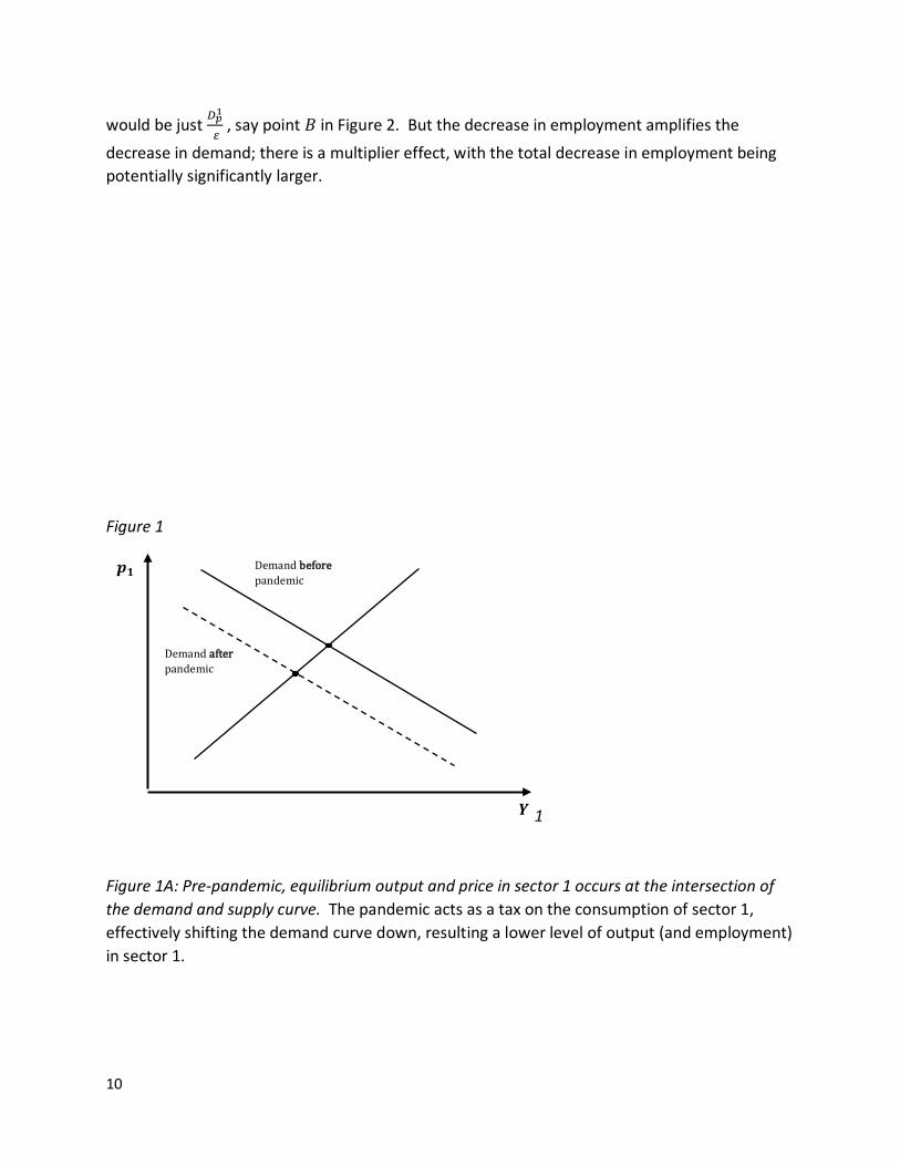
would be just 𝐷𝐷𝑝𝑝1

𝜀𝜀 , say point 𝐵𝐵 in Figure 2. But the decrease in employment amplifies the

decrease in demand; there is a multiplier effect, with the total decrease in employment being potentially significantly larger.

Figure 1

1

Figure 1A: Pre-pandemic, equilibrium output and price in sector 1 occurs at the intersection of the demand and supply curve. The pandemic acts as a tax on the consumption of sector 1, effectively shifting the demand curve down, resulting a lower level of output (and employment) in sector 1.

Demand after pandemic

Demand before pandemic

𝒑𝒑𝟏𝟏

𝒀𝒀𝟏𝟏

11

Figure 1B: The demand curve for sector 1 consists of essential services (the vertical portion of the demand curve) and inessential services. The pandemic shifts the demand curve for the non-essential services down

Figure 2

Post-pandemic, with wages and prices fixed in the short run, the pandemic shifts down the demand for sector 1, and results in a lower level of employment and output. The inability to fulfill one’s demand for good 2 will result in some shifting in demand from good 2 to good 1; but the offsetting increase in demand does not suffice to restore the economy to full employment.

Inessential demand before covid

Essential demand 𝒑𝒑𝟏𝟏

𝒀𝒀𝟏𝟏

Inessential demand after covid

𝑳𝑳𝟏𝟏

𝒀𝒀𝟏𝟏

𝑬𝑬𝟏𝟏

𝑨𝑨

𝑪𝑪

𝑬𝑬𝟏𝟏∗

𝑯𝑯𝟏𝟏

𝑫𝑫𝟏𝟏

𝑩𝑩

𝑫𝑫�𝟏𝟏

12

Partial labor mobility and macroeconomic externalities

This analysis is little changed if labor can move from sector 1 to sector 2, but at a cost, 𝑧𝑧, if wages and prices are fixed. The reason is simple: at the initial equilibrium, 𝑤𝑤2 = 𝑝𝑝2𝐻𝐻2’(𝐿𝐿2), so 𝑤𝑤2 + 𝑧𝑧 > 𝑝𝑝2𝐻𝐻2’(𝐿𝐿2) for all 𝐿𝐿2 > 𝐿𝐿2𝑜𝑜, the initial value of 𝐿𝐿2. It doesn’t pay firms in sector 2 to pay the mobility (training) costs.

But hiring additional workers in sector 2 gives rise to a macroeconomic externality: it generates an increase in employment in sector 1 of

(13) 𝑑𝑑 ln𝐸𝐸1𝑑𝑑𝑑𝑑𝑑𝑑 𝐸𝐸2

= 𝑑𝑑ln 𝐷𝐷1

𝑑𝑑 ln𝑌𝑌2𝜀𝜀−𝜂𝜂

,

and provided 𝑧𝑧 is small enough, a government subsidy to expand output in sector 2 is socially desirable.20

Figure 3 shows how the increase in employment in sector 2 shifts the demand curve for sector 1 up, increasing employment in sector 1.

Figure 3

An increase in employment in sector 2 or in unemployment insurance increases employment in sector 1.

20 The magnitude of the increase in employment in sector 1 is likely to be smaller than given by equation (13), which does not include the indirect effect of the relaxation of the constraint on purchases of good 2 on the demand for good 1. It is straightforward to include this indirect effect in the calculus.

𝑬𝑬�𝟏𝟏 𝑬𝑬𝟏𝟏

𝑯𝑯𝟏𝟏

𝑫𝑫�𝟏𝟏

𝑫𝑫𝟏𝟏

𝒀𝒀𝟏𝟏

𝑬𝑬𝟏𝟏

13

Other Policy shifts

It is easy to see how the provision of unemployment insurance not only ameliorates the suffering of the unemployed, but actually reduces unemployment. Let 𝑏𝑏 be the unemployment benefit provided to unemployed workers. Equation (9) now reads

(14a) 𝐻𝐻1(𝐸𝐸1) = 𝐷𝐷1�𝑝𝑝 + 𝜏𝜏,𝑤𝑤1𝐸𝐸1 + 𝑏𝑏(𝐿𝐿1 − 𝐸𝐸1),𝑤𝑤2𝐿𝐿2;𝐻𝐻2(𝐸𝐸2)�

and it is immediate that an increase in 𝑏𝑏 increases the level of employment in sector 1.21

Increased government expenditures may alleviate the consequences of even a supply side perturbation

While this economic downturn was caused by what might be viewed as a supply side perturbation, a demand side intervention—an increase in government spending—may still reduce unemployment. This is seen most clearly if the government expenditures are focused on sector 1:

(14b) 𝐻𝐻1(𝐸𝐸1) = 𝐷𝐷1�𝑝𝑝 + 𝜏𝜏,𝑤𝑤1𝐸𝐸1,𝑤𝑤2𝐿𝐿2;𝐻𝐻2(𝐸𝐸2)� + 𝐺𝐺1,

where it is immediate that an increase in 𝐺𝐺1 increases 𝐸𝐸1.22 It is worth noting, however, that even an increase in government demand for good 2 will normally increase employment in sector 1, because the supply of sector 2 goods available for consumers will be reduced. For instance, assuming that the government demand for good 2 gets priority, the equilibrium condition for sector 1 is now

(14c) 𝐻𝐻1(𝐸𝐸1) = 𝐷𝐷1(𝑝𝑝 + 𝜏𝜏,𝑤𝑤1𝐸𝐸1,𝑤𝑤2𝐿𝐿2;𝐻𝐻2(𝐸𝐸2) − 𝐺𝐺2)

And so long as a decreased availability of good 2 (in the supply constrained equilibrium) results in an increased demand for good 1, an increase in 𝐺𝐺2 will result in an increase in 𝐸𝐸1.

21 This analysis abstracts from the impact of the deficits used to finance the unemployment insurance (or the taxes now or in the future that might have to be levied). Ricardian equivalence would suggest that these impacts fully offset the direct effect; but both theory and empirical evidence suggest otherwise. In particular, so long as some of the individuals who receive the unemployment benefits are credit constrained, the increase in consumption of these individuals more than offsets the decrease in consumption of those who reduce their consumption as a result of the anticipation of future taxes. See Stiglitz (1988). There is evidence that many of the recipients of unemployment insurance and cash payments are credit constrained. See Chetty et al 2020. 22 Again, we have, of course, assumed that the savings (consumption) rate is fixed, and we have not discussed the implications of the increased indebtedness and/or taxes associated with the increase in 𝐺𝐺. See the discussion in the previous footnote. But even if there is some increase in the savings rate, in an economy with fixed wages and prices, an increase in government purchases of good 2 crowds in private purchases of good 1. Whether this effect is enough to offset the increase in the savings effect depends both on the strength of the Ricardian effect and the degree of substitutability between the two goods.

14

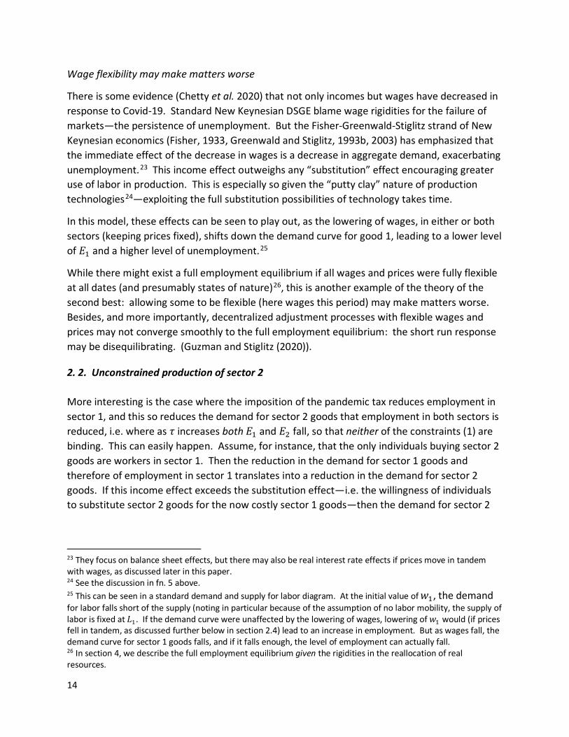
Wage flexibility may make matters worse

There is some evidence (Chetty et al. 2020) that not only incomes but wages have decreased in response to Covid-19. Standard New Keynesian DSGE blame wage rigidities for the failure of markets—the persistence of unemployment. But the Fisher-Greenwald-Stiglitz strand of New Keynesian economics (Fisher, 1933, Greenwald and Stiglitz, 1993b, 2003) has emphasized that the immediate effect of the decrease in wages is a decrease in aggregate demand, exacerbating unemployment.23 This income effect outweighs any “substitution” effect encouraging greater use of labor in production. This is especially so given the “putty clay” nature of production technologies24—exploiting the full substitution possibilities of technology takes time.

In this model, these effects can be seen to play out, as the lowering of wages, in either or both sectors (keeping prices fixed), shifts down the demand curve for good 1, leading to a lower level of 𝐸𝐸1 and a higher level of unemployment.25

While there might exist a full employment equilibrium if all wages and prices were fully flexible at all dates (and presumably states of nature)26, this is another example of the theory of the second best: allowing some to be flexible (here wages this period) may make matters worse. Besides, and more importantly, decentralized adjustment processes with flexible wages and prices may not converge smoothly to the full employment equilibrium: the short run response may be disequilibrating. (Guzman and Stiglitz (2020)).

2. 2. Unconstrained production of sector 2 More interesting is the case where the imposition of the pandemic tax reduces employment in sector 1, and this so reduces the demand for sector 2 goods that employment in both sectors is reduced, i.e. where as 𝜏𝜏 increases both 𝐸𝐸1 and 𝐸𝐸2 fall, so that neither of the constraints (1) are binding. This can easily happen. Assume, for instance, that the only individuals buying sector 2 goods are workers in sector 1. Then the reduction in the demand for sector 1 goods and therefore of employment in sector 1 translates into a reduction in the demand for sector 2 goods. If this income effect exceeds the substitution effect—i.e. the willingness of individuals to substitute sector 2 goods for the now costly sector 1 goods—then the demand for sector 2

23 They focus on balance sheet effects, but there may also be real interest rate effects if prices move in tandem with wages, as discussed later in this paper. 24 See the discussion in fn. 5 above. 25 This can be seen in a standard demand and supply for labor diagram. At the initial value of 𝑤𝑤1, the demand for labor falls short of the supply (noting in particular because of the assumption of no labor mobility, the supply of labor is fixed at 𝐿𝐿1. If the demand curve were unaffected by the lowering of wages, lowering of 𝑤𝑤1 would (if prices fell in tandem, as discussed further below in section 2.4) lead to an increase in employment. But as wages fall, the demand curve for sector 1 goods falls, and if it falls enough, the level of employment can actually fall. 26 In section 4, we describe the full employment equilibrium given the rigidities in the reallocation of real resources.

15

goods will decrease. And this decrease in the demand for sector 2 goods amplifies the initial decrease in the demand for sector 1 goods.

Formally, (7) gives E1 as a function of E2 and (8) gives E2 as a function of E1:

(15a) 𝐸𝐸1 = 𝜃𝜃1(𝐸𝐸2; 𝜏𝜏,𝑤𝑤𝑖𝑖 , 𝑝𝑝)

(15b) 𝐸𝐸2 = 𝜃𝜃2(𝐸𝐸2; 𝜏𝜏,𝑤𝑤𝑖𝑖 , 𝑝𝑝).

We can then solve equations (15) and (16) simultaneously for 𝐸𝐸𝑖𝑖 as a function of 𝜏𝜏, for given {𝑝𝑝,𝑤𝑤𝑖𝑖}:

(16a) 𝐸𝐸𝑖𝑖 = φi(𝜏𝜏;𝑤𝑤𝑖𝑖 ,𝑝𝑝)

We can find conditions under which

(16b) 𝑑𝑑φ𝑖𝑖

𝑑𝑑𝜕𝜕�𝜕𝜕=0

< 0.

Figure 4 illustrates such a case. The initial equilibrium entails 𝜏𝜏 = 0,𝐸𝐸𝑖𝑖 = 𝐿𝐿𝑖𝑖. As Figure 4 illustrates, the pandemic tax shifts the first curve (“Sector 1 equilibrium”) to the left (for any 𝐸𝐸2, the equilibrium employment in the first sector is smaller), and the second curve up (sector 2 equilibrium) (for any 𝐸𝐸1, the equilibrium level of 𝐸𝐸2 has increased.) The magnitude of the respective shifts depends on the substitutability/complementarity between the products as well as the degree of intertemporal substitution, as we have commented on before. At the initial equilibrium, with 𝜏𝜏 = 0, the curves intersect at the initial levels of employment in the two sectors.

16

Figure 4 The pandemic tax can result in unemployment in both sectors. In the case depicted, the new level of employment in both sectors is below the initial level. The decrease in employment in the first sector so depresses demand in the second sector that even though there is some substitutability, overall employment in the second sector is decreased. This is the case of true Keynesian unemployment, of the kind discussed in the earlier work of Delli Gatti et al. (2012a,b). In this case, the mobility constraints are, in a sense, not binding: even though unemployment may be greater in sector 1 than in sector 2, the marginal (unemployed) individual in sector 2 would have little motive to shift, because he would just join the ranks of the unemployed in sector 1.27 Policy: Unemployment benefits and mobility subsidies Providing unemployment benefits, say to the directly affected sector, increases the equilibrium level of employment 𝐸𝐸1, for each value of 𝐸𝐸2; but also increases the equilibrium level of employment 𝐸𝐸2 for each level of 𝐸𝐸1, and results in a higher level of equilibrium employment in both sectors, with potentially large welfare gains. Of course, eventually, such policies encounter the constraints (1), in particular the constraint that 𝐸𝐸2 ≤ 𝐿𝐿2, in which case we shift into the model discussed in the previous section.

27 There will, in general, exist a full employment equilibrium if labor is fully mobile. There may thus exist two (or more) possible equilibria; the “bad” equilibrium reflects a coordination failure. Alternatively, without mobility, there may not exist a full employment equilibrium, for that equilibrium might entail an increase in employment in sector 2, which is precluded by assumption. A third alternative is that there exists an equilibrium with less unemployment, e.g. where there is only unemployment in the first sector, as described earlier.

𝑬𝑬𝟏𝟏

𝑬𝑬𝟐𝟐 sector 1 equilibrium before pandemic

sector 1 equilibrium after pandemic

sector 2 equilibrium before pandemic

sector 2 equilibrium after pandemic

17

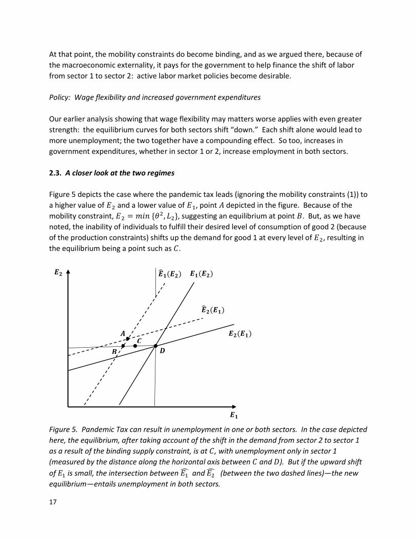
At that point, the mobility constraints do become binding, and as we argued there, because of the macroeconomic externality, it pays for the government to help finance the shift of labor from sector 1 to sector 2: active labor market policies become desirable. Policy: Wage flexibility and increased government expenditures Our earlier analysis showing that wage flexibility may matters worse applies with even greater strength: the equilibrium curves for both sectors shift “down.” Each shift alone would lead to more unemployment; the two together have a compounding effect. So too, increases in government expenditures, whether in sector 1 or 2, increase employment in both sectors. 2.3. A closer look at the two regimes Figure 5 depicts the case where the pandemic tax leads (ignoring the mobility constraints (1)) to a higher value of 𝐸𝐸2 and a lower value of 𝐸𝐸1, point 𝐴𝐴 depicted in the figure. Because of the mobility constraint, 𝐸𝐸2 = 𝑚𝑚𝑖𝑖𝑚𝑚 {𝜃𝜃2, 𝐿𝐿2}, suggesting an equilibrium at point 𝐵𝐵. But, as we have noted, the inability of individuals to fulfill their desired level of consumption of good 2 (because of the production constraints) shifts up the demand for good 1 at every level of 𝐸𝐸2, resulting in the equilibrium being a point such as 𝐶𝐶.

Figure 5. Pandemic Tax can result in unemployment in one or both sectors. In the case depicted here, the equilibrium, after taking account of the shift in the demand from sector 2 to sector 1 as a result of the binding supply constraint, is at 𝐶𝐶, with unemployment only in sector 1 (measured by the distance along the horizontal axis between 𝐶𝐶 and 𝐷𝐷). But if the upward shift of 𝐸𝐸1 is small, the intersection between 𝐸𝐸1� and 𝐸𝐸2� (between the two dashed lines)—the new equilibrium—entails unemployment in both sectors.

𝑬𝑬𝟏𝟏

𝑬𝑬𝟐𝟐 𝑬𝑬𝟏𝟏(𝑬𝑬𝟐𝟐)

𝑬𝑬�𝟐𝟐(𝑬𝑬𝟏𝟏)

𝑬𝑬𝟐𝟐(𝑬𝑬𝟏𝟏)

𝑫𝑫

𝑨𝑨

𝑩𝑩 𝑪𝑪

𝑬𝑬�𝟏𝟏(𝑬𝑬𝟐𝟐)

18

It is apparent from Figure 5 that if the shift up of the curve giving employment in sector 2 as a function of 𝐸𝐸1, is small relative to the shift to the left (effectively down) of the curve giving employment in sector 1 at each level of 𝐸𝐸2, then the pandemic equilibrium will entail a lower level of 𝐸𝐸2 than 𝐿𝐿2, i.e. neither employment constraint will be binding; there will be unemployment in both sectors. 2.4. Flexible prices The analysis so far has assumed fixed wages and prices. Assume now that the pandemic sector is highly competitive and so prices are set so prices are on the firms’ supply curve, so long as the labor constraint is not binding. Then we replace equation (7) and (8) with

(17a) 𝑌𝑌1(𝑝𝑝,𝑤𝑤1) = 𝐷𝐷1�𝑝𝑝 + 𝜏𝜏,𝑤𝑤1𝐸𝐸1,𝑤𝑤2𝐿𝐿2;𝐻𝐻2(𝐸𝐸2)�

(17b) 𝐻𝐻2(𝐸𝐸2) = 𝐷𝐷2 (𝑝𝑝 + 𝜏𝜏,𝑤𝑤1𝐸𝐸1,𝑤𝑤2𝐸𝐸2;𝐻𝐻2(𝐸𝐸2))

where

(17c) 𝐸𝐸1(𝑝𝑝) = 𝐻𝐻−1[𝑌𝑌1(𝑝𝑝,𝑤𝑤1)]

The equilibrium is now described by two equations in the two unknowns {𝑝𝑝,𝐸𝐸2}, as illustrated in Figure 6. The analysis proceeds much as before.28

Figure 6 Equilibrium with flexible prices but rigid wages

28 A natural stability condition ensures that the sector 1 equilibrium locus is flatter than the sector 2 equilibrium locus.

𝑬𝑬𝟐𝟐

𝒑𝒑

Sector 1

Sector 2

19

2.5. Health vs. Macroeconomic externalities and structural Keynesian policies Underlying the analysis so far is the presumption that we wish to reduce unemployment. But what if there are significant health externalities associated with either consumption or production in sector 1, which are obviously not fully reflected in individuals’ decisions about consumption or work? Assume, for instance, that increased consumption of sector 1 has an external health cost of 𝜒𝜒(𝑌𝑌1) which individuals do not take into account in making their demand decisions. We focus on the Keynesian equilibrium where 𝑌𝑌1 is just a function of 𝐸𝐸1, and so for convenience we express the external health cost just as a function of employment in that sector. (This formulation allows the health externality to arise either in the process of consumption or production.) Assume the social welfare function can be expressed simply as a function of 𝐸𝐸1, 𝐸𝐸2, and 𝜒𝜒: 𝑊𝑊(𝐸𝐸1,𝐸𝐸2,𝜒𝜒), with 𝐸𝐸𝑖𝑖 a function of some policy 𝑃𝑃: 𝐸𝐸𝑖𝑖(𝑃𝑃). Then, obviously, optimal policy may entail less than full employment, if

𝑑𝑑𝑊𝑊𝑑𝑑𝑃𝑃 = 𝑊𝑊𝐸𝐸1

𝑑𝑑𝐸𝐸1𝑑𝑑𝑃𝑃 + 𝑊𝑊𝐸𝐸2

𝑑𝑑𝐸𝐸2𝑑𝑑𝑃𝑃 + 𝑊𝑊𝜒𝜒

𝑑𝑑𝜒𝜒𝑑𝑑𝑃𝑃 ≤ 0

At 𝐸𝐸𝑖𝑖 = 𝐿𝐿𝑖𝑖, i.e. at full employment. It is preferable to have some unemployment than to bear the costs of the greater spreading of disease that would result from full employment. But there are policies that can simultaneously help mitigate the disease and its consequences and bolster employment. Assume, for instance, there are public expenditures on sector 2 goods, that reduce the private or social costs of the pandemic, i.e. a category of expenditure, 𝐺𝐺2𝐻𝐻 such that 𝜏𝜏(𝐺𝐺2𝐻𝐻) with 𝜏𝜏’ < 0 and 𝜒𝜒(𝐺𝐺2𝐻𝐻) with 𝜒𝜒𝐺𝐺2𝐻𝐻 < 0, e.g. expenditures on protective gear and tests. It is clear that such expenditures improve welfare on all accounts, increasing 𝐸𝐸𝑖𝑖 and private and public health, and such expenditures should be expanded (if they exist) until the economy reaches full employment. Similarly, we noted earlier that there is a macroeconomic externality associated with moving individuals from sector 1 to sector 2 when sector 2’s employment constraint is binding. For the government to absorb those moving costs may be welfare improving, provided that the external health costs are not too large. In our earlier work, we identified these kinds of expenditures as structural Keynesian expenditures, i.e. there is an underlying set of structural problems (here, associated with the pandemic and the constraints on labor mobility), and expenditures which simultaneously address the structural problem and stimulate aggregate demand do “double duty.” In the aftermath of the Great Depression, expenditures that facilitated the movement of workers from the rural to the urban sector and trained them for jobs in that sector provided a structural Keynesian stimulus.

20

3. Precautionary behavior and intertemporal substitution

The analysis so far can be criticized as being overly simplistic, a black box analysis, simply taking the demand curves as given, not deriving them from first principles, a derivation based on the usual intertemporal maximization problem.29 This has been deliberate. As we have suggested in the introduction, dominating the problem of intertemporal substitution on which standard analyses focus is that of risk and precautionary behavior. Individuals simply don’t know how long and severe the pandemic and its economic aftermath will be. Though under restrictive conditions, one can formulate their decision problem as if they were maximizing expected utility with subjective probabilities, those subjective probabilities have no bases in relative frequencies, and it is problematic whether, confronting the pandemic, that model provides a good description of behavior. What is clear is that upper income individuals (and firms, which we have omitted from the analysis) respond by building up large cash balances, as they confront the risk of an extended period of unemployment with limited assistance from government.30 This precautionary behavior, increasing savings, shifts down the demand curves for both commodities, resulting in a new equilibrium with Keynesian unemployment, i.e. there is a greater presumption that, without government assistance, the situation will be that

29 We described our analysis as taking savings as given. But we could just as easily analyze the equilibrium where savings is endogenous. We can construct a two-period model where, without uncertainty, we can fully derive all demand functions in the standard way, taking into account mobility constraints and the associated supply constraints. Assume the second period (the end of the analysis) wages and prices are fully flexible and resources are fully mobile, so that we have a standard general equilibrium allocation, conditional on the “wealth” that has been transferred from the first period to the second. Assume individuals have rational expectations about that equilibrium. Then for any price vector describing that equilibrium, and for the given wage and price vector describing the initial period, individuals optimally allocate their consumption over the two periods and two goods, simultaneously deciding on how much wealth to convey to the second period. The model of the previous section can be thought of as “solving” this full equilibrium. The analysis of this section then explores the consequences of the increase in savings as a result of risk. 30 I should be clear that not everyone behaves in this way. There are two important exceptions, both of which can be easily accommodated within the framework of this paper. The first are individuals who are credit constrained, who would like to consume more than they do today, and so consume all of their income. Providing more income to them (e.g. temporary benefits in the midst of the pandemic) leads them to consume more. There is evidence that this describes a large fraction of lower income individuals in the United States (Chetty et al 2020), a point that had been emphasized in earlier macro-models emphasizing the importance of distribution (e.g. the models of Pasinetti (1962) or Kaldor (1955), where workers, to a first approximation, consume all of their income); in earlier macro models emphasizing the importance of credit and equity constraints (Greenwald and Stiglitz, 1990, 2003; Weiss and Stiglitz, 1992; Hubbard, 1998), and in the more recent HANK models (Kaplan et al. 2018). The second group are those that may be so depressed by the life prospects under the pandemic that they take the attitude “live while you can.” For these individuals too consumption is only limited by today’s income (and possibly what they can borrow.) In both cases, the presence of large numbers of individuals for whom consumption equals income implies (a) multipliers are larger than otherwise would be the case and (b) income effects may be more important than substitution effects.

21

depicted in Figure 4. The policies described earlier then become applicable. In particular, because of the marked differences in marginal propensities to consume, the expansionary effect of assistance provided to those who are credit constrained will be markedly higher than for assistance provided to upper income individuals. (It is important to recognize that the increase in precautionary behavior results, at least in part, in an increase in demand for non-produced assets, like land and money, not for produced assets, for reasons explained below.) But there is one further set of policies which becomes particularly relevant: reducing the extent of risk aversion. We discuss these policies below. 3.1. Market Failures and the potential for government intervention In standard economics, there is an exercise that one normally performs at this point: Why don’t markets provide the optimal amount of insurance? Why is there a need for government? After all, if individuals are risk averse, won’t private markets have an incentive to provide unemployment insurance? Where’s the market failure? Such exercises made sense forty years ago when there was still a presumption (in some circles) that markets were efficient. But advances in economics should have made clear that there should be a presumption that markets are not efficient (See Greenwald and Stiglitz (1986, 1988), Arnott, Greenwald, and Stiglitz (1994), Geanakoplos and Polemarchakis, 1986) , especially in the presence of imperfect and asymmetric information—obviously central to the concerns here—and there are a wealth of reasons for government intervention. Still, it may be useful to rehearse the standard arguments, since they may, at the same time, provide some guidance for what government policies may be most appropriate. Incomplete risk markets and government interventions Before presenting these arguments, we should give perhaps the most compelling reason for government intervention: markets have often not provided insurance products—like annuities at reasonable prices, health insurance, especially for the aged and without restrictions on pre-existing conditions, and unemployment insurance—and the government has to been able to provide insurance that people value enormously; and even when the private sector provides similar products to those of the public, public insurance typically, even today, has provisions addressing key contingencies, such as inflation. Moreover, the private sector can’t provide for intergenerational risk sharing. Publicly provided social insurance—even with imperfectly designed programs—have enormously increased societal well-being. They have, in particular, enhanced individuals’ security.31

31 For a more extensive discussion of some aspects of government’s advantage in risk-bearing, see Stiglitz (1993).

22

As we look at pandemic-risk from our perspective emphasizing the incompleteness of markets, the absence of pandemic insurance is perhaps not surprising. Nor, given the past behavior of insurance companies, is their attempt to weasel out of the coverage they have provided for business interruption insurance—one of the few pandemic related risks that seemed to be covered, absent the ambiguous fine print which the insurance companies now want to be read in their favor. While the absence of insurance coverage for events that have not been well-contemplated—like the current lock-downs associated with Covid-19—is perhaps understandable, it is worth noting that now, after the risks are amply clear, markets are still not stepping up to pool and share the risks going forward. While there may not be well-defined probabilities for each of the relevant risks that will determine the course of disease and its economic impact (e.g. around the discovery of vaccines and therapeutics), in standard economic models that should not be required for the establishment of markets to share and pool risks. Yet, these events, of enormous consequence for the lives of everyone, remain largely uninsurable. Explaining the absence of insurance markets Central to the Guzman-Stiglitz analysis was the assumption of incomplete contract: one simply cannot specify, with any clarity—and especially with sufficient clarity to have an enforceable contract—insurance contracts providing for every possible relevant contingency, especially with the differentiated treatment that each circumstance “deserves,” and would have in a world with complete contracting. Because insurers know that there are risks beyond those that they can easily contemplate, typical insurance contracts have provisions limiting coverage to specified risks (those not specified are not covered) and explicitly limiting coverage for important risks, the magnitude of which are hard to ascertain ex ante, and especially those which may simultaneously affect many individuals—i.e. have macroeconomic significance. Thus, as we noted, most insurance companies are claiming that their coverage of business interruption insurance does not extend to the interruptions associated with the pandemic. Moreover, even when there is coverage, when there are large macroeconomic disturbances (i.e. events which simultaneously affect large numbers of households and firms), private insurance firms often don’t have the financial wherewithal to deliver the benefits promised. This is an example of the macroeconomic inconsistencies emphasized by Guzman and Stiglitz (2020): events like crises and pandemics entail promises not being fulfilled. Rationally, individuals (except those living in the world of DSGE models) know this, but they do not and cannot know what will happen when these contracts are broken. They do not and cannot know the outcome of bankruptcy proceedings, or the extent to which Courts will recognize arguments like force majeure or necessity, providing an “out” for those not fulfilling contract terms.

23

In addition, there are the standard limitations on insurance markets presented by adverse selection and adverse incentives. Advantages of government vs. private sector While the government faces similar problems arising from information asymmetries and the impossibility of specifying complete contracts, there are telling differences, both in instruments and objectives. For instance, the government is concerned about macro-economic externalities; the private sector is not; and as Greenwald and Stiglitz (1986) pointed out, economies with imperfect information and incomplete contracts/markets are rife with micro- and macro-externalities. The government has the power to proscribe and incentivize actions (e.g. through taxes and regulatory policies) that are not available to private actors. And the governments’ ability to redistribute ex post—after it sees the roll of the dice—allows it to mitigate social risks in ways that the private sector simply can’t. Obviously, knowing that there is going to be some ex post redistribution has incentive effects, but they are mixed in nature: on the one hand, it may lead to more entrepreneurial risk taking and mitigate macroeconomic externalities such as those that arise from excessive precautionary savings; on the other hand, it may encourage more corelated risk taking, and it may, in some circumstances, lead to excessive risk taking (the infamous moral hazard problem.) In the absence of insurance for critical contingencies—in this case, for “states of nature” depending on the pace and evolution of the disease and the development of vaccinations and therapeutics, the provision of recovery measures by the US and other governments, and the effectiveness of those measures in restoring the (relevant) economies (sectors) to full employment—individuals will tend to save more and in forms which have more “flexibility,” e.g. in liquid assets, whose value may be perceived to be uncorrelated, or even better, negatively correlated, with possible adverse outcomes. It is the uncertainties, as we have said, that will dominate behavior, more than intertemporal smoothing. 3.2. Intertemporal substitution vs. Risk The contrast in perspectives can be seen most clearly in the case where the pandemic is known to disappear next period.32 Then, in a two-period model, we can think of any individual as having a utility function of the form (in the obvious notation)

(18) 𝑈𝑈 = 𝑈𝑈(𝐶𝐶11,𝐶𝐶12,𝐶𝐶21,𝐶𝐶22)

32 We discuss this case further in the next section.

24

Standard macro-economic models make the empirically dubious assumption of time separability. But just as a thought experiment, consider the case where individuals only care about their life-time consumptions of the two goods, i.e. the utility function takes the form

(19) 𝑈𝑈 = 𝑈𝑈(𝐶𝐶11 + 𝐶𝐶12,𝐶𝐶21 + 𝐶𝐶22)

Then knowing that there is a tax on consuming good 1 only in the first period, if goods prices don’t adjust in an offsetting way, they would consume good 1 only in period 2 and good 2 in period 1. In the absence of adjustment costs, and say with a linear production function, the economy would remain at full employment and the pandemic (as modeled here—apart from its direct effect on health) would have no economic effect, though it would have a large effect on intertemporal patterns of consumption. More generally, with knowledge that the disease will “just disappear,” there is no need for increasing precautionary behavior: all one has to do is to do as well as one can in rearranging patterns of consumption over time. Real rigidities (costs of reallocating resources) and nominal rigidities (difficulties in adjustments in prices and wages) can give rise to the kinds of short run costs that we have delineated in this paper. Indeed, the presence of these rigidities, taking them as given, gives rise to a macroeconomic externality associated with savings: each individual believes, for instance, that by postponing consumption of good 1 to next period, he can avoid paying the “pandemic tax,” but as they all do this, employment in the first sector, and possibly in both sectors, decreases. Society as a whole pays a cost in terms of underutilization of resources. Simple Analytics In short, the demand functions used earlier (equations (7) and (8)) need to be extended not just to incorporate possibly constraints on purchases of good 2 but also an increase in precautionary savings to reflect the uncertainty posed by pandemic and the possible desire to postpone consumption until a period when the pandemic tax is not being levied. We thus write the demand (this period) for good 𝑖𝑖 as

(20) 𝐷𝐷𝑖𝑖(𝑝𝑝 + 𝜏𝜏,𝑤𝑤1𝐸𝐸1,𝑤𝑤2𝐸𝐸2;𝐻𝐻2(𝐿𝐿2); 𝑠𝑠(𝜏𝜏,𝜎𝜎))

where we have assumed that the savings rate is a function of the magnitude of the pandemic tax and the uncertainty associated with the future, 𝜎𝜎. The effect of an increase in 𝑠𝑠 can be easily traced out in either of the two cases: In the case where there is full employment in the second sector, the increase in uncertainty shifts down 𝐷𝐷1, leading to a lower level of 𝐸𝐸1. In the case where there is unemployment in both sectors, the increase in uncertainty shifts down both 𝐷𝐷1 and 𝐷𝐷2, leading to decreased employment in both sectors.

25

3.3. Why it matters Whether one prioritizes the analysis of risk and uncertainty makes a difference, because it naturally draws one’s attention to different kinds of policy measures. Misplaced emphasis on wage rigidities When it is assumed that the only important deviations from a perfectly competitive equilibrium model are wage (and price) rigidities, we are naturally led to the policy recommendation: if we could only make wages flexible enough, we could restore full employment; and by making wages more flexible—weakening unions or reducing severance pay—welfare is improved. We’ve already shown that making wages more flexible—but not fully flexible—could in fact worsen the problem: a dynamic theory of the second best. Guzman and Stiglitz argued the problem of unemployment was more one of excessive volatility in aggregate demand than of insufficient wage flexibility; that is, reasonable institutional reforms, like the installation of automatic stabilizers and capital controls, are more likely to enhance stability and full employment than weakening unions or job protections. Misplaced emphasis on intertemporal substitution So too, the focus on intertemporal substitution—individuals maximizing their intertemporal utility, with lifetime budget constraints—naturally puts a focus on intertemporal prices, interest rates. The hope was that the lowering of interest rates by monetary authorities would induce higher levels of aggregate demand now, restoring full employment. With substitution and income effects moving in offsetting ways, and with large numbers of individuals being target savers—saving for retirement, to buy a house, or to put their children through school—for whom lowering of interest rates leads to lower levels of consumption, it was never obvious why so many economists thought this was likely to be a power instrument for stimulating the economy, especially in a deep downturn. Though the limits of monetary policy have now once again (as they were in the earlier days of Keynesian thought) become part of conventional wisdom, it is not (as the standard models suggest) because of the “zero lower bound.” There are ways, using time profiles of sales taxes and investment credits, to change intertemporal prices, even in the presence of the ZLB. Rather, it is simply that changes in the real interest rate in the relevant range do not have the required impact on aggregate demand. Large enough changes (along the lines described below) might.33

33 Monetary policy can, of course, work through other channels, e.g. on credit availability or through exchange rate effects. Part of the lack of ability of monetary policy to stimulate the economy in the 2008 crisis was related to the failure to increase lending to those parts of the economy (SME’s) facing credit constraints. Changes in exchange rates are, of course, “beggar thy neighbor” policies, improving aggregate demand in one country at the expense of that in others.

26

3.4. Policies to encourage consumption (or investment) in the presence of risk Recognizing that at least part of the fundamental problem is risk and the failure of risk markets—and as a result, in a fundamental sense, individual risk may well exceed societal risk --draws attention to what policy can do to reduce risk, thereby reducing the demand for precautionary balances and increasing consumption today. Policies which strengthen unemployment insurance (or other welfare support programs) and making a commitment that such expanded programs will be available so long as the unemployment rates remain elevated reduce individuals’ needs for precautionary balances. (Thus, the refusal, as this paper goes to print, of the Republicans in the US to support such a commitment is counterproductive.34) There are measures that could directly reduce the risk confronting those making investment decisions (either of consumer durables or productive assets): state-contingent (income contingent) loans, where the amounts to be paid back next period (and possibly over the life of the asset) depend on the state of the pandemic and/or the income (profits) of the individual (firm). These can be thought of as “partial Arrow Debreu securities,” socializing some of the risk associated with these expenditures in ways that markets have failed to do so, and doing so with terms that recognize the macroeconomic externalities associated with these investments.35 The standard analysis rests on confounding two matters that should be kept separate. First, time and risk. The weakness in consumption today is not the result of too high an interest rate, but of the absence of insurance against some potentially very adverse circumstances in the future. The presence of macroeconomic externalities means, moreover, that individual and social incentives are not well aligned. We’ve described a couple of ways that public policy may address directly the risk problem.

34 The claim that the benefits are excessive, and are resulting in a labor shortage, seems dubious. As we have explained, the decrease in jobs in say airlines, restaurants, and other contact service sectors arises from the pandemic “tax.” Having more people search for jobs that don’t exist doesn’t increase the level of employment. Many individuals are reluctant to work given the risks that that imposes on them, for which they are not adequately compensated. If markets worked well, employers could still find workers, even if there were generous unemployment benefits, but, of course, they would have to pay higher wages. Cross state evidence (based on differences in unemployment benefits) corroborates this perspective. See Altonji et al. 2020. 35 One can think of these loans as making a commitment to provide additional liquidity in the event, say, that the unemployment remains high next period. But the provision of such liquidity at such a time would obviously not be inflationary: by definition, it is a time of insufficient aggregate demand. One can design contracts where there is little or no moral hazard: the individual or firm would still have to repay the loan at some later date, when the economy recovered.

27

There are also ways that government policy may more directly encourage consumption or investment today, in a more targeted and effective manner than an overall change in the interest rate. Some countries have already implemented such programs: a “sale” on consumption or investment goods today, encouraging consumption and investment today. This can be done through time dated consumption coupons, or through a temporary investment tax credit or a temporary lowering of the sales tax on, say, cars. Such measures may be desirable if one believes that there is irrational pessimism which is preventing consumption today. The problem with the pandemic is that risk perceptions may be rational. The increase in consumption this period comes at the expense of lower cash balances, and if, next period, the risk remains unabated, individuals may be even more anxious, and double down on building up their precautionary balances. That is why, given that the underlying problem is one of risk, measures which socialize this risk seem better targeted. There is a second confusion: between the holding of precautionary balances with produced vs. non-produced goods. The standard models have at most one non-produced good, money. In general, there is a form of Say’s Law in action: when individuals decide to consume more at a later date, they want there to be the productive capacity to produce that good, and so investment increases in tandem. But if individuals take today’s income and hold it in the form of land or money, there is no offsetting increase in the demand for goods produced today. Supply does not create its own demand. One of the reasons for the limited efficacy of the vast increase in liquidity in 2008, or in 2020, is that so little of it went into the demand for produced goods and so much of it went into holdings of money and of pre-existing assets, giving rise to increases in asset prices. Again, government policies can, at least at the margin, shift the demand away from non-produced assets to those currently being produced, e.g. increasing capital gains taxes on a mark to mark basis, for investments in pre-existing assets without provisions for the deductibility of losses. Such a policy would change the relative price of a pre-existing asset and a new asset, encouraging the production of new capital goods. 3.5. Credit constraints and precautionary balances An important feature of the economy is that different individuals are in different circumstances. A significant fraction has no cash balances and is living paycheck to paycheck. For these individuals, a reduction in income has to translate into a reduction in expenditures. There is little or no scope for precautionary balances. For these, the savings rate is zero. But there is another group who are not living quite on the edge, who are saving, and who respond to the pandemic by increasing precautionary balances. The data we cited in the introduction concerning the average savings rate shows that a large portion of the population (weighted by income) was not credit constrained, and did not become credit constrained by the pandemic—though this was almost surely partly because of the large government programs.

28

(The national income data may not fully reflect what is happening to household balance sheets. With the stay on evictions, large fractions of the population have not paid their rents. Their cash balances have gone up—but so too have their liabilities.) The fact that some individuals are credit constrained and others not needs to be reflected in our model for the demand for goods and services. Instead of (21) we write

(21a) 𝐷𝐷𝑖𝑖(𝑝𝑝 + 𝜏𝜏,𝑤𝑤1𝐸𝐸1,𝑤𝑤2𝐸𝐸2;𝐻𝐻2(𝐿𝐿2); 𝑠𝑠(𝜏𝜏,𝜎𝜎), 𝜆𝜆)

where 𝜆𝜆 is the fraction of the population that is credit constrained.

There is one important policy implication of this formulation: if we can target money towards credit constrained individuals, the multiplier effect will be larger than untargeted money, much of which will simply go into increased precautionary balances. Chetty et al. show, in fact, that spending increased significantly upon the receipt of government checks in April, 2020.

So too, even the stay on evictions can not only alleviate the immediate suffering resulting from the pandemic, but also stimulate the economy: in effect, it loosens the credit constraints facing individuals. But such stays have more ambiguous effects in the intermediate run (discussed briefly below in section 4): household balance sheets weaken (in a way which is not the case with direct payments), meaning that the post pandemic recovery will be more difficult. To mitigate these effects, what is needed is not just a stay, but a temporary rent/interest rate reduction. After all, had the pandemic been anticipated, and had there been more complete contracts, there would likely have been provisions calling for a reduction in rents and interest payments during the pandemic.

3.6. Investment

So far, we have ignored investment. It is easy to introduce investment, 𝐼𝐼. It is natural to think of investment as related to sector 2, and for simplicity, we limit it to that. Then we replace (8) by

(22) 𝐻𝐻2(𝐸𝐸2) = 𝐷𝐷2(𝑝𝑝 + 𝜏𝜏,𝑤𝑤1𝐸𝐸1,𝑤𝑤2𝐸𝐸2) + 𝐼𝐼

So long as 𝐼𝐼 is fixed and unaffected by the pandemic, the analysis is unchanged. But 𝐼𝐼 will be affected, through several channels: (a) Lower expected output next period in either sector 1 or sector 2 (as a result of the continuation of the pandemic) will depress investment today36; (b) Lower profits in either sector with cash/credit/equity constrained firms will result in lower investment; (c) Increased uncertainty about the future will result in lower investment; and (d)

36 This effect can be incorporated formally into the model by assuming that 𝐼𝐼 = 𝐼𝐼(𝑌𝑌1,𝑌𝑌2;𝑟𝑟) where 𝑟𝑟 is the interest rate. In the Keynesian equilibrium described in earlier sections, 𝑌𝑌𝑖𝑖 = 𝐻𝐻(𝐸𝐸𝑖𝑖). This increases the macroeconomic externality from sector 1 to sector 2 and vice versa, and implies a larger decrease in both 𝐸𝐸1 and 𝐸𝐸2.

29

risk averse banks will be less willing to lend (and possibly less able to lend, if there are significant defaults), and will change the terms of lending to make borrowing less attractive.37 It is thus possible that post-pandemic, the level of 𝐸𝐸2 corresponding to any level of 𝐸𝐸1 may actually be lower, in which case it is unambiguously the case that both 𝐸𝐸1 and 𝐸𝐸2 will have decreased. While monetary policy may attempt to counteract these forces, with interest rates already near zero, the ability of it to do so (if it ever could) is limited. Moreover, the increase in uncertainty may lower the elasticity of investment with respect to interest rate: at no interest rate (in the relevant range) will investment be large enough to restore full employment.

Note that our analysis here follows the standard Keynesian approach in emphasizing that the savings and investment decisions are made independent of each other (unlike in much of the contemporary macroeconomics literature, where firms don’t even exist as independent institutions). In the background, there is one further distinction, perhaps not sufficiently emphasized by Keynes: the decision to save may create a demand for a non-produced asset, like land. (See the discussion below in section 5).

3.7. Open economy

So far, we’ve modeled a closed economy. The analysis can be easily modified to incorporate trade. We do so in a very reduced form way. For simplicity, we assume only sector 2 is traded, and net exports 𝑋𝑋 are a function of 𝑝𝑝, 𝜏𝜏, the exchange rate 𝑒𝑒 and the constraint 𝐻𝐻2(𝐿𝐿2), if it is binding: 𝑋𝑋 = 𝑋𝑋(𝑝𝑝, 𝜏𝜏, 𝑒𝑒;𝐻𝐻2(𝐿𝐿2)). Net exports must equal capital inflows, 𝐹𝐹, which depend on variables like the interest rates in the two countries, and beliefs about the rate of change of the exchange rate, which in turn are affected by beliefs about the future evolution of the economy. In this pandemic (as in other crises), initially there was a flight to safety—capital flows into the US, leading to an appreciation of the currency. With interest rates close to zero, monetary policies play a less important role. As time goes on, it becomes clearer how the pandemic will affect different countries. With the US performing more poorly than many other countries, it is perhaps not surprising that the exchange rate has declined. We formalize the exchange rate determination by

(23) 𝑋𝑋�𝑝𝑝, 𝜏𝜏, 𝑒𝑒;𝐻𝐻2(𝐿𝐿2)� = 𝐹𝐹(𝑒𝑒, 𝜏𝜏;𝛺𝛺)

where 𝛺𝛺 represents beliefs about the future (next period), and in particular about next period’s exchange rate.

Now, the goods market equilibrium in sector 2 becomes

(24) 𝐻𝐻2(𝐸𝐸2) = 𝐷𝐷2(𝑝𝑝 + 𝜏𝜏,𝑤𝑤1𝐸𝐸1,𝑤𝑤2𝐸𝐸2) + 𝐼𝐼 + 𝑋𝑋

37 There are still other channels: if prices and wages are flexible, there will be further adverse effects on balance sheets, given that firms’ debts are not indexed. The fall in wages and prices increases the real interest rate, and this may discourage investment.

30

(7), (23) and (24) are then solved simultaneously for {𝐸𝐸1,𝐸𝐸2, 𝑒𝑒}. Adding, for instance, government expenditure to the demand for good 2 or a universal cash payment or unemployment benefits (as earlier), we can ascertain impacts on the level of employment in both sectors. For a country like the United States which imports much of its durable manufacturing goods, the concern is that any untargeted spending support will go to increase the demand for imports (given the unattractiveness of non-essential services in the midst of the pandemic).38 If capital inflows are relatively inelastic, the major impact will be on the exchange rate, not on aggregate demand. More generally, net imports will increase from what they otherwise would have been, but not as much as they would have done in the absence of the exchange rate adjustment; and the increased net imports will partially offset the direct expansionary effect of the government program.39 This suggests that the time-dated targeted service vouchers described earlier may be a more effective way of supporting the economy. 3.9. Covid-19 and labor supply This paper has focused on the impacts of Covid-19 on demand; but it also can have supply side effects. Many workers are reluctant to work in jobs in which they may be exposed to Covid-19. We could model that as a tax on working in the first sector during Covid-19, with the labor supply schedule given by 𝐿𝐿𝑖𝑖 = 𝐿𝐿𝑖𝑖(𝑤𝑤1 + �̂�𝜏),𝐿𝐿𝑖𝑖′ < 0,𝐿𝐿𝑖𝑖(𝑤𝑤1𝑜𝑜) = 𝐿𝐿, where 𝑤𝑤1𝑜𝑜 is the first sector wage in the initial equilibrium. In the initial cases considered here, where wages are rigid, the tax leads to a reduction in the supply of labor to the first sector. This reduces the potential supply in the first sector. There are then two cases: (a) that where the initial fall in demand is greater than the fall in supply. The analysis follows exactly as in earlier sections. Some of those “unemployed” in the first sector have left voluntarily and are looking for jobs at the going wage in the second sector. (b) that where the initial fall in supply is greater than the fall in demand. Then there is still a macroeconomic externality from the first sector to the second, now driven by the supply side. The reduced income in the first sector still leads to reduced demand in the second sector. The supply constraint in the first sector shifts up the demand function in the second sector (just as the supply constraint in the second sector affected the demand for first sector goods.) Thus, in the case where there is Keynesian unemployment in the second sector, the magnitude of that unemployment is less than would have been the case with the same level of first sector employment. Subsequent adjustments, however, are markedly different in this case than in that studied earlier. Now, there is upward pressure on wages in the first sector, rather than downward 38 Jamie Galbraith has emphasized this in his analysis of the Covid-19 response. 39 On a seasonally adjusted basis, the trade balance in goods went from -$60 billion in February to -$81 billion in July 2020, a one third increase, and at an annual rate representing some 1% of GDP. (The balance of trade in goods and services worsened even more, from -$37 billion to -$64 billion.)

31

pressures. As wages rise, demand in both sectors increase. But there is still downward pressure on wages in the second sector. Depending on the relative pace of adjustment in the two sectors, demand may increase or decrease. If it decreases, it has no effect on the first sector, since output in that sector is supply constrained. Eventually, of course, the demand constraint will become binding, and then we merge into case (a). Meanwhile, the fall in wages in sector 2 exacerbates the deficiency of aggregate demand in that sector, lowering employment and output. On the other hand, if aggregate demand increases, whether the discrepancy between aggregate demand and supply in the first sector increases or decreases depends on the magnitudes of the demand and supply effects, which in turn depend on the income elasticity of the demand for good 1 vs. the labor supply elasticity. Either is possible. At the same time, the increase in aggregate demand in sector 2 increases employment there, which has a macro-economic externality of increasing demand in sector 1. Matters can be more complicated with income demand elasticities of workers in the two sectors possibly differing. We leave the various possible patterns as exercises for the reader. There are two important points raised by the analysis: (a) as in our earlier analysis, decentralized adjustments may not be equilibrating; but (b) at least in sector 1 we should see upward wage pressures rather than downward. Early evidence from a number of studies (including Cajner et al. 2020) shows significant wage declines, and especially in the most affected sectors, suggesting that the labor supply constraint is not binding.40

4. Short-short run, short run, intermediate run vs. Long Run Pandemic Analysis The analysis in section 2 focused on the first period equilibrium, assuming that savings were fixed. In section 3, we discussed how savings might be affected, both through intertemporal substitution and as a result of risk. It is clear how an increase or decrease in savings alters the equilibrium analysis of section 2.

40 If labor supply responses to covid-19 were driving the economic downturn, as David Vines has emphasized, one could use a one-sector model to depict the macroeconomic consequences. It is, in effect, a temporary downward shift in the labor supply curve, which has an income effect (life time income is lower) which is smoothed out through shifting consumption/spending forward in time—so the decrease in demand might be expected to be less than the decrease in supply were it not for the decrease in investment (assuming prices remain unchanged.) But the decrease in output over the duration of the pandemic means (if the pandemic lasts long enough) that there will be a decrease in investment. Moreover, if monetary policy remains unchanged, the increased uncertainty leads to a shift in demand towards precautionary assets—money and land—and away from physical capital goods, depressing investment still further. If, as we described above, the labor shortage was the predominating effect in the short run, the upward pressure on wages might lead monetary authorities following inflation targeting policies to increase interest rates, exacerbating the shortfall in aggregate demand.

32

Here, we focus on four additional aspects. The impacts in the short and medium term depend critically on whether covid-19 will pass, and (as we noted in the last section) on the uncertainty about when that might happen. Even if Covid-19 were to be a permanent (or long lasting) feature of life, short run impacts can differ from long run because of adjustment costs. We have assumed that in the short run, wages and prices are fixed. We have noted that in practice, they adjust, but such adjustments do not necessarily bring the economy closer to full employment. Below, we describe the full employment equilibrium that would emerge if wages and prices were fully flexible, and somehow, the economy could find itself in this full employment equilibrium. More interesting though than this hypothetical is a look at the short run dynamics likely to unfold as the economy emerges from the pandemic, with the devastation that it brings to the economy: hysteresis affects abound. 4.1. Some complexities in consumption patterns: Adaptation Indeed, interpreting on-going data on consumption—trying to make inferences from that data for what patterns of consumption might look like in the future—is difficult, partly because of the uncertainties that we have just discussed, and partly because of the large adjustments to which the pandemic has given rise. “Adjustment” effects should not be confounded with longer range effects. For instance, the pandemic has, as our model emphasized, given rise to changed patterns of activities. New activities may require investments, either by firms or consumers. Individuals no longer go to gyms, and so their demand for bicycles and home exercise equipment has soared. In urban centers like New York, where the subway may be viewed as unsafe and where there is demand for open spaces where one can enjoy the outdoors without masks, there is an increase in demand for cars. Many homes have had to upgrade the quality of their wi-fi. But these are one-time investments that mask the overall concern about increasing precautionary balances. (There has, in fact, been a huge increase in such balances on the part of both corporates and households.) Of course, there are still a large number of individuals who live on the edge. These are individuals for whom the changes in current income incorporated in our model are likely to be particularly significant; and for whom government subsidies are likely to give rise to corresponding large increases in spending. 4.2. Contrasting Implications of a short-term vs a longer term pandemic The analysis changes in several ways if individuals know that the pandemic is only a short-term phenomenon. First, the willingness to expend resources on investments for patterns of behavior which are assumed to be only temporary will be limited. Thus, the kinds of expenditures described in the previous subsection will be more limited.

33

Secondly, the impact of the pandemic on consumption in the short run may be different, possibly even more adverse. As we have modeled it, the tax becomes a tax on consumption of sector 1 goods only in the first period. As we have already noted, this will distort consumption not only towards sector 2 in the first period, but also towards the second period. One can avoid the tax simply by delaying eating in restaurants to the next period. In this case, savings in the first period will increase. Of course, in a full equilibrium model, individuals should know that if, say, there are capacity constraints next period (i.e. the economy was already at full employment in the second period), then they can’t enjoy more consumption then unless there is more investment today. Presumably, the intertemporal prices would adjust (assuming full price flexibility) and/or monetary policy would lower the interest rate, to encourage consumption today. But, as we noted in the previous section, the required degree of price flexibility and the required adjustments in interest rates are unlikely to be forthcoming. Besides, under plausible assumptions, the lowering of interest rates will lead to increased savings—individuals have to save more to provide for the retirement, to make the down payment on their house, or to pay for their children’s education. Given the high level of uncertainty, and pervasive credit and equity rationing, firms may not increase investment, certainly not enough to ensure full employment in the first period. In a dynamic disequilibrium model, however, individuals may not fully understand all the constraints—they may formulate dynamically inconsistent plans. Hence, they do set aside more today for future consumption. And even more so if there is uncertainty about the duration of the pandemic and its economic impacts.41 4.3. The long run: a new full employment equilibrium? In the long run, one might assume that all wages and prices are adjustable, and all factors are mobile. But such assumptions are far from innocuous.42 Nominal wages and prices might adjust, but in a decentralized economy, they might adjust in such a way as to give rise to rigidities in relative wages and prices, i.e. relative wages and prices that do not ensure full employment. (Solow and Stiglitz (1968)). Even if eventually wages and prices exhibited full employment, that could be a long, long time. And in economies with asymmetries in information—all economies—there can be rigidities in real wages and real interest rates.

41 It is straightforward to model optimal consumption behavior in a world in which there is a Poisson probability that the pandemic disappears every period. See the Appendix for a simple two period model of savings under uncertainty, using standard subjective utility analysis. That model, however, almost surely does not adequately capture fully the extent to which the pandemic engenders precautionary behavior, discussed further in section 3. . Kreps (1979, 1992) provides a better framework for analyzing choice in the presence of the kinds of uncertainties posed by the pandemic 42 Moreover, in the time scale of such adjustments, other “state” variables are likely to change—not just the state of the pandemic, but capital stocks, labor supplies, and firm net worth.

34

Still, even in the presence of the labor market rigidities restricting labor mobility, we can determine the wages and prices which would give rise to full employment. The supply of labor in each sector is fixed (at 𝐿𝐿𝑖𝑖), so full employment simply requires the demand for good 𝑖𝑖 to be equal to the full employment supply, in the absence of rationing:

(25) 𝐻𝐻𝑖𝑖(𝐿𝐿𝑖𝑖) = 𝐷𝐷𝑖𝑖(𝑝𝑝 + 𝜏𝜏,𝑤𝑤1𝐿𝐿1,𝑤𝑤2𝐿𝐿2)

Equilibrium requires that firms in the two sectors want to hire, at the going wages and prices, the labor which is available in the sector

(26) 𝑤𝑤2 = 𝐻𝐻2′(𝐿𝐿2)

(27) 𝑤𝑤1 = 𝑝𝑝𝐻𝐻1′(𝐿𝐿1)

(26) implies that 𝑤𝑤2 is unchanged, (27) that 𝑤𝑤1/𝑝𝑝 is unchanged, so that (25) then becomes a single equation in a single unknown, 𝑝𝑝. A sufficiently large fall in the price of the good adversely affected by the pandemic (good 1), with a correspondingly large fall in the wage of workers in that sector may restore full employment.43 Of course, this sets in motion, over the longer term, a movement of workers from sector 1 to sector 2, and the restoration of a new general equilibrium, reflecting the new “technology” whereby there is a pandemic cost to the consumption of good 1. (It also will set in motion forces for the development of technologies where good 1 can be consumed without bearing as high a pandemic cost.)

The various policy instruments that we have described (reducing risk, increasing unemployment benefits, moving individuals from sector 1 to sector 2) reduce the magnitude of the reduction of 𝑝𝑝 required to attain full employment, and if full employment is not attained, the extent of unemployment.

4.4. Post-pandemic dynamics and macroeconomic externalities

The analysis has been, for the most part (with the exception of the previous subsection), very short run. We have described some of the forces at play that may or may not reduce unemployment in the short run. For instance, the presence of unemployment in sector 1 may lead to lower wages, and this may actually exacerbate the unemployment problem; while the movement of workers from sector 1 to sector 2 may, under some circumstances, reduce the unemployment rate (though not in others). We have described the full employment equilibrium, but whether such an equilibrium will be quickly attained without government intervention is not clear. What is clear is that there may be large macroeconomic externalities, so that government intervention will, in general, be desirable.

43 This is not quite accurate. Even at a price of zero, consumption of good 1 may be so unattractive at least for some individuals that demand is less than what would be supplied with full employment.

35

There are many aspects of macroeconomic externalities and the dynamics of adjustment that have been explored in the broader macroeconomic literature and are relevant for the analysis here, which has put particular emphasis on incomplete contracts and markets.

In particular, the economic downturn in sector 1, and possibly in sector 2, has adverse implications for the balance sheets of firms and workers in those sectors. Following along the lines of analysis of Greenwald-Stiglitz (1993a), there will be an increase in the risk of bankruptcy, with the loss of organizational and informational capital that results, not just from the increased risk associated with the pandemic but also because of these adverse effects on balance sheet. Increased risk, worsened balance sheets, and depleted organizational and informational capital in turn, will lead to decreased investment and even have adverse effects on firms’ willingness to produce. Combined with weaker household balance sheets, both aggregate supply and demand shift down, lowering employment and output, with effects which persist even after the pandemic has been controlled. That is, even if it were known that the pandemic would “just disappear” after one period, the effects of the pandemic could live on after. Government interventions during the pandemic to mitigate the magnitude of the downturn would reduce these adverse effects and thus would yield benefits not just during the pandemic, but also in its aftermath.

So too, if the pandemic makes labor-intensive production in certain sectors less attractive, and there is uncertainty about the duration of the pandemic, and firms respond by installing robots, then once the pandemic is put under control, the demand for labor will be lower than it otherwise would have been, and inequality is likely to be higher. If there are (perhaps costly) government interventions that can simultaneously limit the spread of the disease even with labor-intensive technologies, those interventions may be socially desirable.

Pandemics quintessentially entail externalities, so there is no presumption that market responses to a pandemic are Pareto efficient. And the macroeconomic consequences of decentralized responses to the pandemic, in the presence of incomplete contracts and markets in a disequilibrium world with learning, naturally give rise to large macroeconomic externalities, and again there is a presumption that well-designed interventions are welfare enhancing, even when the government has no more information about the course of the evolution of the pandemic than the agents within the economy.

4.5. A one sector model

We have argued that central to understanding the impact of Covid-19 on the economy is understanding the differential impacts on different sectors and different groups (low income workers who are credit constrained vs. high income workers who engage in precautionary savings). It is useful as a thought experiment to ask, what the impact would be in a one sector economy, where Covid-19 either makes consumption today (and for the duration of the pandemic) less attractive, or makes work less attractive. This kind of perturbation can easily be handled within standard DSGE models, as a temporary shift in the functions describing the

36

utility of consumption or the disutility of work. We do not go through the formalities, but discuss the qualitative results.

If there were only one sector, and say the pandemic exercised its effect by making work less attractive at any wage (since it increases the exposure to Covid-19), then a temporary pandemic would, at a fixed wage and intertemporal prices, reduce permanent income, and thus consumption, less than today’s aggregate supply; while employment would decrease, there would be no unemployment, and indeed there would be labor shortages and upward pressure on wages, contrary (as we noted) to what has been observed.

If there were only one sector, and the pandemic exercised its effects by making consumption less attractive at any price, then, at fixed wages and prices, including interest rates, the pandemic would lead to a reduction in demand and employment. There would be no Keynesian multiplier, since lifetime income, which determines consumption in the standard model, would be largely unaffected. One might have thought that, given that the marginal benefits to consuming more today are lower, it makes sense that individuals work less today. But especially with more general utility functions, individuals might want to smooth work over time, so that there is no close link between changes in the marginal utility of consumption at any date and the desired level of work at that date.44 Hence, individuals might not want to change their level of work much, even though they want to change their consumption levels a great deal. There could be considerable unemployment. It could take large adjustments in wages and prices (including intertemporal prices) to restore full employment.

As we noted earlier, standard monetary policy adjustments in those cases where the dominant effect of the pandemic is through discouraging labor supply would discourage consumption and investment today, exacerbating the unemployment. Conversely, in those cases where the effects come through consumption, and there is an increase in unemployment, the lowering of interest rates as inflationary pressures are reduced (deflationary pressures increased) will increase aggregate demand and serve to restore the economy to full employment. But whether the policy response is fast enough and the behavioral response to that policy response is large enough (or even in the right direction) to counteract the downward pressures, which result directly from the disinflation/deflation discussed in section 3.6, is ambiguous.

5. Dynamic Disequilibrium Models with Noise

In an earlier paper, we presented an alternative approach for the study of macroeconomics to the standard Dynamic Stochastic General Equilibrium (DSGE) model that has become fashionable in economics, which we referred to as a Dynamic Disequilibrium Model with Randomness. (Guzman and Stiglitz, forthcoming).

44 Obviously, one can construct utility functions for which consumption today and leisure today are either complements or substitutes, i.e. the drop in consumption today because of the pandemic leads to an increase or decrease in labor supply. In the latter case, there could again be a labor shortage (at the given set of wages and prices). In the former case, the increase in the unemployment rate is even greater.

37

Nothing could better illustrate the differences in approaches than the disturbance associated with Covid-19, generating the largest economic collapse in memory. In its nature, it is closer to the kinds of shocks envisaged in the standard DSGE models—an exogenous “technology” shock—than to the demand/financial shock of either the Great Recession, the 1991 downturn, or even the Great Depression. But clearly, though there was ample warning of the threat of a pandemic and an awareness of the possible cost—under President Obama, the White House had set up within the National Security Council an office for Pandemic preparedness—and a few scholars had attempted to estimate the magnitude of the risks (suggesting that they might be comparable to that associated with global warming (Fan et al. 2016)), none of the standard DSGE models incorporated the risks into their analyses, nor did many individuals, enterprises, and financial institutions. The pandemic was not just the realization of one of the many possible states of nature, all anticipated, with well defined (subjective) probabilities corresponding to the objective frequencies describing the occurrence of this kind of pandemic. Once it became clear that we were in the midst of a pandemic, there was still no “common knowledge”: perceptions about the evolution of the disease and its economic impact differed markedly within the population and across countries. There was an enormous amount of learning. This learning affected behavior—and changes in behavior affected in turn the behavior of the economic system.45

It was clear in this crisis, and in that of 2008, that the cognitive dissonance that marks DSGE modelling, whereby individuals believe, or at least act as if, there economy is always on an equilibrium trajectory (in which the transversality condition is satisfied), even in those moments immediately after it is clear that they were not on an equilibrium trajectory, and have to recalibrate—and this is so no matter how often such disturbances occur—did not describe well the unfolding events: the economy did not immediately go onto a new equilibrium trajectory. There was a real process of groping—of trying to understand what had happened and what would unfold, through an interaction between policymakers, the political system, and other agents in the economy and the political and social system. In the case of the 2008 Great Recession, as was true in the Great Depression, it would be almost a decade before the economy returned to something approaching full employment. In 2008, there was not common knowledge concerning the shocks that gave rise to the crisis or the impacts of the policy responses.46 Writing now, in the midst of the Covid-19 pandemic, we simply don’t know the course of the disease; and there are large disagreements about the desirability, and even consequences, of alternative policies.

45 It is important to realize that as learning occurs, the behavior of the economic system changes, and that there are no general theorems concerning the efficiency or stability of alternative learning processes. Indeed, Dosi et al. (2020) and Siniskaya and Tesfatsion (2015) have recently demonstrated that what might seem “better” learning processes—using more sophisticated estimation processes compared to more myopic expectations—actually result in poorer systemic performance. Catullo, Gallegat and Russo (2020) have shown that while more sophisticated learning systems may improve firm performance, macroeconomic performance may be worsened. 46 Eighty years after the Great Depression, there is still not a fully agreed understanding of that event.

38

Six critical features defined our approach and differentiated it from DSGE, all of which are illustrated by the pandemic.

First, and most importantly, we argued that, in the absence of futures markets for all states of nature going infinitely far into the future, the world was such that individuals were typically not on long run equilibrium paths satisfying the transversality conditions at all dates and all states.

That in turn implied that there would be moments—typically revealed at times of critical macroeconomic dysfunction, like financial crises—in which macroeconomic inconsistencies became apparent, where individuals’ plans were not, and in many cases, could not, be fulfilled.

These were moments that often were not fully anticipated, and in many cases not even contemplated. Certainly, the details of how the relevant events would play out was not thought through. Accordingly, not only was there not a complete set of Arrow-Debreu securities, contracts themselves were incomplete in a fundamental way.

A defining feature of the pandemic is that many contracts are being broken, with follow on effects that are still unknown. And as we noted, the few insurance contracts covering some of the consequences (business interruption insurance) are being contested.

Thirdly, these moments are points of time in which individuals learn a great deal about the world—about the economy and the political system which governs it. The rational expectations model—in which all states are anticipated, and life is but a playing out of the rolls of the dice that nature affords—simply does not apply. There are large changes in views about what is possible and what is likely. No one before the pandemic would have contemplated that there were circumstances, outside of war, where governments would be willing to undertake deficits of the magnitude that we have seen. Few had contemplated downturns of the magnitude and rapidity that have been experienced.

Fourthly, the momentary equilibrium was typically associated with at least some markets not clearing, most importantly the labor market: unemployment was real, and not just caused by nominal wage rigidities. Nominal wages might be flexible, though obviously, in a sense, not flexible enough. Most importantly, as we have shown, the theory of the second best applies: increased flexibility might make matters worse.

In our earlier paper, we had argued that what really needed to be explained was not the inflexibility of wages but the volatility of aggregate demand: were aggregate demand more stable, there was sufficient wage flexibility that the economy might have been able to remain at or near full employment. Though it is no surprise that the pandemic has given rise to a very large change in aggregate demand, there is still something to explain: why intertemporal substitution didn’t do a better job in stabilizing aggregate demand. Part of the explanation, we have suggested, lies in the increased precautionary behavior that is central to our disequilibrium analysis. This precautionary behavior exacerbated the economic downturn.

39

Fifth, the adjustment processes, the responses of economic agents to this learning, does not put them onto a new dynamic equilibrium path. Decentralized adjustments could move them further away either from a momentary equilibrium in which all markets clear and/or a dynamic equilibrium in which transversality conditions are satisfied in all states and dates. There was no presumption that a decentralized market economy was either efficient or stable, and there were government interventions that were welfare improving.

Finally, because there are alternative stores of value—money or land—if individuals save more, the demand for “future” consumption does not translate into an increased demand for produced goods today (capital goods). It can lead instead to an increase demand for money or land or gold or other non-produced goods, leading (as Keynes suggested) to a deficiency of aggregate demand today, a deficiency which is not easily or quickly remedied by decentralized adjustments in prices or even by government adjusting interest rates. These non-produced goods may be particularly desirable at times of great uncertainty, where the very nature of the future economy is so much up in the air, for they provide more “flexibility,” i.e. they are likely to have value regardless of what emerges (See Kreps, 1979, 1992). By contrast, the value of any specific capital good—whether an airplane or a machine—may be far more uncertain.

The critique of the DSGE model, of course, is not just that the assumptions which go into it are implausible, but are directed at its ability to explain and predict, and to provide guidance on policies to prevent and respond to fluctuations. DSGE models have systematically failed to predict the large macroeconomic perturbations, like the 2008 crisis, and to provide adequate policy responses to the events which have such monumental consequences. In most of the cases, the disturbances are endogenous—rather than the exogenous technology shocks that are the source of the perturbations in DSGE models. Our analysis suggests that they are equally unsuited for thinking about responses to the pandemic, which is, in some ways, more like the technology shocks upon which the models focus. It is, for instance, exogenous. Today, individuals and firms are not thinking about the sequence of consumption and investments that ensure that they are on an equilibrium path with full macroeconomic consistency, with all transversality conditions satisfied. They are thinking about the unknown and unknowable course of the disease and the economy, and how to protect themselves against what may lie ahead. While individuals and firms do not just live in the moment—they think forward—they respond to current signals, aware of the limits of their knowledge. Government interventions that are based on this more realistic model of behavior are likely to prove more successful than those based on alternative hypotheses.

6. Concluding Comments

In this paper, we have modeled Covid-19 as an unanticipated technology shock that adversely affects the demand for good 1—it acts as a tax on its consumption—for a period of unknown duration, with unknown and uncertain effects on the economy, with unknown and uncertain policy responses—and unknown and uncertain responses of the agents within the economy to those policy responses. But given the sluggish adjustment of prices and wages (and possibly

40

expectations about future values of those variables), and the real rigidities in the economy, the technology shock can give rise to Keynesian unemployment, where government Keynesian policy responses—such as increased government expenditures and unemployment subsidies—can help restore full employment. Under some circumstances, Keynesian structural policies—expenditures aimed at reallocating labor—can be helpful. Second best economics prevails: trying to make labor markets more flexible may make matters worse.

While we have focused on a pandemic shock affecting the consumption of certain sectors (here, sector 1), we have shown how the analysis can easily be extended as well to a pandemic shock affecting certain production technologies, e.g. those employing workers working in close quarters.

So too, as we have suggested, the analysis can be extended to models with multiple sectors, where some are adversely (positively) affected not just by the income and substitution effects upon which we have focused, but also by cross elasticities, including those arising from binding demand and supply constraints (the inability to obtain certain goods; the inability to “sell” as much labor as one would like.)

There has never been an event like this in the era of modern industrialization, so, even if we understood more about the virus, it is natural that we don’t know about how economic agents and the economic system respond. There is much learning. Not surprisingly, we have learned that there are markedly different views about how economic agents and the economic system respond, and markedly different views of how, under these unique circumstances, agents and the system will respond to different policy interventions. The world is not well-described by common knowledge, and any model which makes the assumptions of rational expectations, common knowledge, and the economy being on an equilibrium trajectory, is not likely to provide a good basis either for predicting what will happen or for designing optimal policy responses. The lockdowns were designed not only to reduce the imposition of externalities by individuals on each other, to reduce the spread of the disease directly during the period of the lockdown, but also to induce changes in behavior. But the extent to which they were able to induce changes in behavior was greatly affected by the information, or disinformation, to which individuals were exposed. Understanding how policies affect beliefs and behavior is central to understanding the efficacy of alternative policies.

Hopefully, this paper has not only provided some insights into the evolution of the economy in response to the pandemic and the design of appropriate policy responses, but also has made a convincing case that the approach to macroeconomics explored by Guzman and Stiglitz, “The Dynamic Disequilibrium Model with Randomness”, with its emphasis on learning, disequilibrium, and a decentralized adjustment process provides a useful framework for dealing with those large and not fully understood events that seem to so frequently interrupt the smooth workings of capitalist economies, whether they are debt or financial crises, pandemics, or terrorist attacks.

41

In such circumstances, attention has to be drawn to the key determinants of behavior at those moments, with attention to policies which might be the most effective in restoring the economy quickly to full employment. We have stressed that unemployment largely arises from the fact that the immediate effect on aggregate demand is felt faster than the impacts of the sluggish response of wages and prices, and because those responses are done in an uncoordinated, decentralized manner, they may well be disequilibrating. Thus, the focus of attention should be on ameliorating the adverse shock to aggregate demand, if possible, in ways that address some of the structural problems that have given rise to the underlying unemployment. Well targeted policies are likely to be more effective, and increase social welfare, more than broad based “bazookas” such as that unleashed by the CARES Act in the US. Policies which address extremes of precautionary behavior, including the demand for money, land, and other non-produced assets, may be particularly effective at such moments of extreme uncertainty; we have described several such policies. In particular, we have emphasized the importance of providing assurances that supportive policies will be continued as long as the underlying weaknesses in the economy persist. Even if monetary policy were not at its limits, times of extreme uncertainty are times where the interest elasticity of consumption and investment are likely to be very low, so that monetary policy is not likely to be very effective. There will have to be a reliance on fiscal policy. At such times, fiscal policy may be particularly effective: if Ricardian effects are ever relevant, they are especially unlikely to be relevant at these junctures, where individuals are focused on the here and now, not on long run transversality conditions, and where credit constraints are likely to be especially relevant for large portions of households and firms. The wide divergence of behavioral responses between those households who are credit constrained and those that are not suggests that targeting assistance to the former will have a much larger multiplier. Targeting expenditures that address the underlying problem—protective gear and tests that help prevent the spread of the disease—have triple benefits: direct benefits in containing the disease, structural benefits in reducing what we have modeled as the “pandemic tax,” and Keynesian benefits in reducing unemployment.

References

Atkinson, A. B. and J. E. Stiglitz, 1969. “A New View of Technological Change,” Economic Journal, 79(315), September, pp. 573-578.

Altonji, Joseph, Zara Contractor, Lucas Finamor, Ryan Haygood, Ilse Lindenlaub, Costas Meghir, Cormac O’Dea, Dana Scott, Liana Wang, and Ebonya Washington. 2020. “Employment Effects of Unemployment Insurance Generosity During the Pandemic.” Yale University, July 14.

Arnott, Richard, Bruce C. Greenwald, and Joseph E. Stiglitz. 1994. “Information and Economic Efficiency.” Information Economics and Policy, 6 (1): 77–88.

42

Autor, David H., David Dorn and Gordon H. Hanson. 2013. “The China Syndrome: Local Labor Market Effects of Import Competition in the United States.” American Economic Review, 103 (6): 2121–68.

_______2016. “The China Shock: Learning from Labor-Market Adjustment to Large Changes in Trade.” Annual Review of Economics 8: 205–40.

Barro, Robert, and Herschel I. Grossman. 1971. “A General Disequilibrium Model of Income and Employment.” American Economic Review, 61 (1): 82–93.

Cass, David, and Joseph E. Stiglitz. 1969. “The Implications of Alternative Saving and Expectations Hypotheses for Choices of Technique and Patterns of Growth.” Journal of Political Economy 77 (July-August 1969), 586–627.

Catullo, Ermanno, Mauro Gallegati, and Alberto Russo, 2020. "Forecasting in a complex environment: Machine learning sales expectations in a Stock Flow Consistent Agent-Based simulation model," Working Papers 2020/17, Economics Department, Universitat Jaume I, Castellón (Spain).

Chetty, Raj, John N. Friedman, Nathaniel Hendren, Michael Stepner, and the Opportunity Insights Team. 2020. “How Did COVID-19 and Stabilization Policies Affect Spending and Employment? A New Real-Time Economic Tracker Based on Private Sector Data.” NBER Working Paper No. 27431. Updated https://opportunityinsights.org/wp-content/uploads/2020/05/tracker_paper.pdf.

Delli Gatti, Domenico, Mauro Gallegati, Bruce C. Greenwald, Alberto Russo and Joseph E. Stiglitz. 2012a, “Mobility Constraints, Productivity Trends, and Extended Crises.” Journal of Economic Behavior & Organization, 83 (3): 375–393.

__________2012b. “Sectoral Imbalances and Long Run Crises.” In The Global Macro Economy and Finance, eds. Franklin Allen, Masahiko Aoki, Jean-Paul Fitoussi, Nobuhiro Kiyotaki, Roger Gordon, and Joseph E. Stiglitz, Houndmills, UK and New York: Palgrave, 61–97.

Dixit, Avinash and Robert Pindyck. 1994. Investment Under Uncertainty, Princeton: Princeton University Press.

Dosi, Giovanni, Mauro Napoletano, Andrea Roventini, J. E. Stiglitz, and Tania Treibich, 2020 “Rational Heuristics? Expectations and Behaviors in Evolving Economies with Heterogeneous Interacting Agents,” Economic Inquiry 58 (3): 1487–1516.

Farhi, Emmanuel, Isabel Correia, Juan Pablo Nicolini, and Pedro Teles. 2013. “Unconventional Fiscal Policy at the Zero Bound.” American Economic Review 103 (4): 1172–1211.

Fan, Victoria Y., Dean T. Jamison, and Lawrence H. Summers. 2016. “The Inclusive Cost of Pandemic Influenza Risk,” NBER Working Paper No. 22137.

43

Fisher, Irving. 1933. “The Debt Deflation Theory of Great Depressions,” Econometrica, 1 (4), 337–357.

Geanakoplos, John D., and Heraklis M. Polemarchakis. 1986. “Existence, Regularity, and Constrained Suboptimality of Competitive Allocations when the Asset Market Is Incomplete.” In Uncertainty, Information and Communication: Essays in Honor of K. J. Arrow, eds. W. Heller, R. Starr, and D. Starrett, Cambridge, UK: Cambridge University Press, 65–96.

Greenwald, Bruce C., and Joseph E. Stiglitz. 1986. “Externalities in Economies with Imperfect Information and Incomplete Markets.” Quarterly Journal of Economics, 101 (2): 229–64.

_______ 1988. “Pareto Inefficiency of Market Economies: Search and Efficiency Wage Models.” American Economic Review, 78 (2): 351–55.

______1990. “Macroeconomic Models with Equity and Credit Rationing,” with Bruce C. Greenwald. In Asymmetric Information, Corporate Finance, and Investment, ed. R. Glenn Hubbard, Chicago: University of Chicago Press, 15–42.

______1993a. “Financial Market Imperfections and Business Cycles.” Quarterly Journal of Economics, 108 (1): 77–114.

_____1993b. “New and Old Keynesians.” Journal of Economic Perspectives 7 (1): 23–44.

_____2003. Towards a New Paradigm in Monetary Economics, with Bruce Greenwald. Cambridge: Cambridge University Press.

Guzman, Martin and Joseph E. Stiglitz. 2020. “Towards a Dynamic Disequilibrium Theory with Randomness,” NBER Working Paper No. 27453.

Hubbard, R. Glenn. 1998. “Capital-market imperfections and investment,” Journal of Economic Literature 36 (1): 193–225.

Kaldor, Nicholas. 1955. “Alternative Theories of Distribution.” Review of Economic Studies, 23 (2): 83–100.

Kaplan, Greg, Benjamin Moll, and Giovanni L. Violante. 2018. “Monetary Policy According to HANK.” American Economic Review, 108 (3): 697–743.

Kreps, David M. 1979. “A Representation Theorem for ‘Preference for Flexibility’.” Econometrica, 47 (3): 565–577.

Kreps, David M. 1992. “Static Choice in the Presence of Unforeseen Contingencies,” Economic Analysis of Markets and Games: Essays in Honor of Frank Hahn. Cambridge: MIT Press. Malinvaud, Edmond. 1977. The Theory of Unemployment Reconsidered (Yrjö Jahnsson Lectures). Oxford, UK: Blackwell.

44

Pasinetti, Luigi L. 1962. “The Rate of Profit and Income Distribution in Relation to the Rate of Economic Growth,” Review of Economic Studies, 29 (4): 267–79. Sinitskaya, Ekaterina and Tesfatsion, Leigh, (2015), Macroeconomies as constructively rational games, Journal of Economic Dynamics and Control, 61, issue C, p. 152-182 Solow, Robert M., and Joseph E. Stiglitz. 1968. “Output, Employment and Wages in the Short Run.” Quarterly Journal of Economics 82 (4): 537–560.

Stiglitz, Joseph. 1969. “Behavior Toward Risk With Many Commodities,” Econometrica, 37 (4): 660–667.

_______ 1988. “On the Relevance or Irrelevance of Public Financial Policy.” In The Economics of Public Debt, Proceedings of the 1986 International Economics Association Meeting, eds. Kenneth Arrow and Michael Bostin, London: Macmillan Press, 4–76.

_______ 1993. “Perspectives on the Role of Government Risk-Bearing within the Financial Sector.” In Government Risk-Bearing, ed. Mark S. Sniderman, Norwell, MA: Kluwer Academic Publishers, 109-130. _______ 2011. “Rethinking Macroeconomics: What Failed and How to Repair It.” Journal of the

European Economic Association, 9 (4): 591–645.

_______ 2016. Towards a General Theory of Deep Downturns: Presidential Address to the 17th World Congress of the International Economic Association in 2014, Houndmills, UK and New York: Palgrave Macmillan.

______ 2018. “Where Modern Macroeconomics Went Wrong.” Oxford Review of Economic Policy 34 (1–2): 70–106.

_______2020. “The Economy of Tomorrow: Recovering and Restructuring after COVID-19” Roosevelt Institute Policy Brief, October

Stiglitz, Joseph E., and Andrew Weiss. 1992. “Asymmetric Information in Credit Markets and Its Implications for Macroeconomics.” Oxford Economic Papers, 44 (4): 694–724.

Yagan, Dan. 2019. “Employment Hysteresis from the Great Recession.” Journal of Political Economy, 127 (5): 2505–2558.

45

Appendix: Determination of precautionary balances

The standard model of savings under uncertainty has savings chosen to maximize

𝑉𝑉(𝑞𝑞1, (1 − 𝑠𝑠)𝑌𝑌1) + 𝛿𝛿𝐸𝐸𝑉𝑉(𝑞𝑞2, 𝑠𝑠𝑌𝑌1(1 + 𝑟𝑟) + 𝑌𝑌2),

s.t. 𝑠𝑠 ≥ 0, where 𝑉𝑉 is the indirect utility function, 𝑌𝑌𝑖𝑖 income in period 𝑖𝑖 and 𝑞𝑞𝑖𝑖 is the price vector in period 𝐼𝐼, including the pandemic tax, i.e. 𝑞𝑞𝑖𝑖 = 𝑝𝑝𝑖𝑖 + 𝜏𝜏. We focus on the fact that 𝑌𝑌2 and 𝑞𝑞2 are unknown—the individual doesn’t know the extent of economic devastation of the pandemic nor its duration.

Standard models without uncertainty focus on the smoothing of consumption. Here we focus on the effects of uncertainty. Consider, for instance, an individual who believes that he will be unemployed next period. Assume, for simplicity that 𝑟𝑟 = 0 and that the pandemic will continue to next period, so 𝑞𝑞1 = 𝑞𝑞2.47 Then 𝑠𝑠 = ½. Of course, if he were to believe that there was a zero probability of unemployment, then 𝑠𝑠 = 0. The uncertainty associated with 𝑌𝑌2 implies an increase in 𝑠𝑠 provided 𝑉𝑉𝑌𝑌𝑌𝑌𝑌𝑌 > 0.

Notice that the properties of the utility function that determine savings in the presence of uncertainty are different from those that are critical in models without risk. Parameterizations like constant elasticity utility functions which might provide a good approximation for behavior in normal times may be inappropriate in the presence of an extreme event like a pandemic, where individuals may be more concerned about large downside deviations.48

More realistically, because individuals have no basis for judging what are reasonable probability distributions for 𝑌𝑌2, they may focus on worst-case or near worst-case scenarios, which, as we have just shown, can lead to very high savings rates.

47 Alternatively, assume 𝑉𝑉𝑞𝑞𝑌𝑌 = 0.𝑉𝑉𝑞𝑞 = −𝐶𝐶1𝑉𝑉𝑌𝑌, so −𝑌𝑌𝑉𝑉𝑞𝑞𝑌𝑌

𝑉𝑉𝑞𝑞= −𝑅𝑅 + 𝜇𝜇, where 𝑅𝑅 is the elasticity of marginal utility and

𝜇𝜇 is the income elasticity of commodity 1. Note that in this simple model, if there is a probability that the pandemic will end next period, so in effect 𝑞𝑞2 < 𝑞𝑞1, then savings will be higher if 𝑅𝑅 > 𝜇𝜇. 48 There is another more subtle critique of constant elasticity utility functions. In general, the elasticity of marginal utility is not invariant to relative price, as illustrated by the calculations in the previous footnote. More generally, utility functions exhibit constant elasticity at all prices (within a range) only under stringent conditions which are empirically not satisfied. See Stiglitz (1969).