The Ordinary Differential Equations Project
335
The Ordinary Differential Equations Project
Transcript of The Ordinary Differential Equations Project

The Ordinary Differential EquationsProject


The Ordinary Differential EquationsProject
Thomas W. JudsonStephen F. Austin State University
DRAFT March 28, 2018 DRAFT

© 2013–2017 Thomas W. Judson
Permission is granted to copy, distribute and/or modify this document under the terms ofthe GNU Free Documentation License, Version 1.3 or any later version published by the FreeSoftware Foundation; with no Invariant Sections, no Front-Cover Texts, and no Back-CoverTexts. A copy of the license is included in the section entitled “GNU Free DocumentationLicense”.

Preface
This text is intended for an undergraduate course in ordinary differential equations. TheOrdinary Differential Equations Project began when the author was teaching the ordinarydifferential equations course at Harvard University. After arriving at Stephen F. AustinState University, the Harvard notes began to transform into the makings of a textbook.At the same time, the author was converting his abstract algebra book, Abstract Alge-bra: Theory and Applications (http://abstract.pugetsound.edu/index.html) from LaTeXinto MathBook XML (http://mathbook.pugetsound.edu). With MathBook XML, which isnow PreTeXt, one can produce HTML and PDF versions of a textbook as well as manyother formats while only having to maintain the PreTeXt source.
There has been a strong tend during the past few decades to incorporate technologyinto undergraduate differential equations courses. Since it is easy to insert computationalcells inside an HTML version of the textbook with PreTeXt, there is now an opportunityto seemlessly embed technology into the textbook. Sage (sagemath.org), our technolgy ofchoice, is a free, open source, software system for advanced mathematics. Sage is ideal forassisting with a study of ordinary differential equations, since it cannot only be embeddedas computational cells in a textbook, it can also be used on a computer, a local server,or on CoCalc (https://cocalc.com). The Sage code in The Ordinary Differential EquationsProject has been tested for accuracy with the most recent version available at this time:Sage Version 7.6 (released 2017–03–25).
There are additional exercises or projects at the ends of many of the chapters. Someof the projects may require a basic knowledge of programming. All of these exercises andprojects are more substantial in nature and allow the exploration of new results and theory.
Thomas W. JudsonStephen F. Austin State UniversityNacogdoches, Texas 2017
v

Acknowledgements
This book was written in PreTeXt.
vi

Contents
Preface v
Acknowledgements vi
1 A First Look at Differential Equations 11.1 Modeling with Differential Equations . . . . . . . . . . . . . . . . . . . . . . 11.2 Separable Differential Equations . . . . . . . . . . . . . . . . . . . . . . . . 161.3 Geometric and Quantitative Analysis . . . . . . . . . . . . . . . . . . . . . . 281.4 Analyzing Equations Numerically . . . . . . . . . . . . . . . . . . . . . . . . 381.5 First-Order Linear Equations . . . . . . . . . . . . . . . . . . . . . . . . . . 501.6 Existence and Uniqueness of Solutions . . . . . . . . . . . . . . . . . . . . . 631.7 Bifurcations . . . . . . . . . . . . . . . . . . . . . . . . . . . . . . . . . . . . 71
2 Systems of Differential Equations 812.1 Modeling with Systems . . . . . . . . . . . . . . . . . . . . . . . . . . . . . 812.2 The Geometry of Systems . . . . . . . . . . . . . . . . . . . . . . . . . . . . 912.3 Numerical Techniques for Systems . . . . . . . . . . . . . . . . . . . . . . . 1022.4 Solving Systems Analytically . . . . . . . . . . . . . . . . . . . . . . . . . . 111
3 Linear Systems 1183.1 Linear Algebra in a Nutshell . . . . . . . . . . . . . . . . . . . . . . . . . . . 1183.2 Planar Systems . . . . . . . . . . . . . . . . . . . . . . . . . . . . . . . . . . 1243.3 Phase Plane Analysis of Linear Systems . . . . . . . . . . . . . . . . . . . . 1333.4 Complex Eigenvalues . . . . . . . . . . . . . . . . . . . . . . . . . . . . . . . 1393.5 Repeated Eigenvalues . . . . . . . . . . . . . . . . . . . . . . . . . . . . . . 1483.6 Changing Coordinates . . . . . . . . . . . . . . . . . . . . . . . . . . . . . . 1523.7 The Trace-Determinant Plane . . . . . . . . . . . . . . . . . . . . . . . . . . 1633.8 Linear Systems in Higher Dimensions . . . . . . . . . . . . . . . . . . . . . . 1733.9 The Matrix Exponential . . . . . . . . . . . . . . . . . . . . . . . . . . . . . 183
4 Second-Order Linear Equations 1944.1 Homogeneous Linear Equations . . . . . . . . . . . . . . . . . . . . . . . . . 1944.2 Forcing . . . . . . . . . . . . . . . . . . . . . . . . . . . . . . . . . . . . . . 2024.3 Sinusoidal Forcing . . . . . . . . . . . . . . . . . . . . . . . . . . . . . . . . 2144.4 Forcing and Resonance . . . . . . . . . . . . . . . . . . . . . . . . . . . . . . 221
vii

viii CONTENTS
5 Nonlinear Systems 2425.1 Linearization . . . . . . . . . . . . . . . . . . . . . . . . . . . . . . . . . . . 2425.2 Hamiltonian Systems . . . . . . . . . . . . . . . . . . . . . . . . . . . . . . . 2545.3 More Nonlinear Mechanics . . . . . . . . . . . . . . . . . . . . . . . . . . . . 2665.4 The Hopf Bifurcation . . . . . . . . . . . . . . . . . . . . . . . . . . . . . . . 282
6 The Laplace Transform 2976.1 The Laplace Transform . . . . . . . . . . . . . . . . . . . . . . . . . . . . . 2976.2 Solving Initial Value Problems . . . . . . . . . . . . . . . . . . . . . . . . . 3026.3 Delta Functions and Forcing . . . . . . . . . . . . . . . . . . . . . . . . . . . 3076.4 Convolution . . . . . . . . . . . . . . . . . . . . . . . . . . . . . . . . . . . . 311
A GNU Free Documentation License 315
Readings and References 323
Index 325

1
A First Look at DifferentialEquations
1.1 Modeling with Differential EquationsCalculus tells us that the derivative of a function measures how the function changes.An equation relating a function to one or more of its derivatives is called a differentialequation. The subject of differential equations is one of the most interesting and usefulareas of mathematics. We can describe many interesting natural phenomena that involvechange using differential equations. In addition, the theory of the subject has broad andimportant implications.
1.1.1 Exponential GrowthWe begin our study of ordinary differential equations by modeling some real world phenom-ena. For a particular situation that we might wish to investigate, our first task is to writean equation (or equations) that best describes the phenomenon. Suppose that we wish tostudy how a population P (t) grows with time t. We might make the assumption that aconstant fraction of population is having offspring at any particular time. If we also assumethat the population has a constant death rate, the change in the population ∆P during asmall time interval ∆t will be
∆P ≈ kbirthP (t)∆t− kdeathP (t)∆t,
where kbirth is the fraction of the population having offspring during the interval and kdeathis the fraction of the population that dies during the interval. Equivalently, we can write
∆P
∆t≈ kP (t),
where k = kbirth − kdeath. Since the derivative of P is
dP
dt= lim
∆t→0
∆P
∆t,
the rate of change of the population is proportional to the size of the population, or
dP
dt= kP. (1.1)
The equationdP
dt= kP
1

2 CHAPTER 1. A FIRST LOOK AT DIFFERENTIAL EQUATIONS
is one of the simplest differential equations that we will consider. The equation tells us thatthe population grows in proportion to its current size. It is not too difficult to see thatP (t) = Cekt is a solution to this equation, where C is an arbitrary constant. Indeed, if wedifferentiate P (t), we obtain
d
dtP (t) = kCekt = kP (t).
In addition, if we know the value of P (t), say when t = 0, we can also determine the valueof C. For example, if the population at the time t = 0 is P (0) = P0, then
P0 = P (0) = Cek·0 = C
or P (t) = P0ekt. The differential equation
P ′(t) = kP (t),
P (0) = P0
is an example of an initial value problem, and we say that P (0) = P0 is an initialcondition. Since the solution to equation (1.1) is P (t) = Cekt, and we say that thepopulation grows exponentially.
As an example, suppose that P (t) is a population of a colony of bacteria at time t,whose initial population is 1000 at t = 0, where time is measured in hours. Then
1000 = P (0) = Ce0 = C,
and our solution becomes P (t) = 1000ekt. If the population grows at three percent perhour, then
1030 = P (1) = 1000ek,
after one hour. Consequently,k = ln 1.03 ≈ 0.0296
and the solution to our initial value problem is
P (t) = 1000e0.0296t.
Of course, it is important to realize that this is only a model. If t is small, our model mightbe reasonably accurate. However, if we let t be very large, our colony of bacteria could verywell exceed the mass of the earth.
The growth rate of a population need not be positive. For example, Japan has expe-rienced negative growth in recent years.1 The equation dP/dt = kP can also be used tomodel phenomena such as radioactive decay and compound interest—topics which we willexplore later.
To summarize, we say that the expression x(t) = Cekt is a general solution of theequation x′ = kx, and x(t) = x0e
kt is a particular solution to the differential equation.The general solution to our equation x(t) = Cekt graphs as an infinite family of curves,which we will call integral curves or solution curves (Figure 1.1).
1See http://data.worldbank.org/indicator/SP.POP.GROW.

1.1. MODELING WITH DIFFERENTIAL EQUATIONS 3
-2 -1 1 2t
-300
-200
-100
100
200
300
x(t)
x(t) =Cekt
Figure 1.1: Integral curves
1.1.2 Logistic GrowthNot all populations grow exponentially; otherwise, a bacteria culture in a petri dish wouldgrow unbounded and soon be much larger than the size of the laboratory. To see whathappens if there are limiting factors to population growth, let us consider the populationof fish in a children’s trout pond. The number of trout will be limited by the availableresources such as food supply as well as by spawning habitat. A small population of fishmight grow exponentially if the pond is large and food is abundant, but the growth ratewill decline as the population increases and the availability of resources declines. We canuse the logistic equation to model population growth in a resource limited environment.2
To see how the logistic model works, let us try to adjust our model of exponential growthto account for the limited resources of the pond. We will make the following assumptions.
• If the population of trout is small and the pond is large with abundant resources, therate of growth will be approximately exponential,
dP
dt≈ kP.
• If N is the maximum population of trout that the pond can support, then any popu-lation larger than N will decrease. In other words,
dP
dt< 0
for P > N . We say that N is the carrying capacity for the population.
Our assumptions suggest that we might try an equation of the form
dP
dt= kf(P )P,
2The logistic model was first used by the Belgian mathematician and physician Pierre François Verhulstin 1836 to predict the populations of Belgium and France.

4 CHAPTER 1. A FIRST LOOK AT DIFFERENTIAL EQUATIONS
where f(P ) is a function of P that is close to 1 if the population is small, but negative ifthe population is greater than N . The simplest function satisfying these conditions is
f(P ) =
(1− P
N
).
Thus, the logistic population model is given by the differential equation
dP
dt= k
(1− P
N
)P.
Example 1.2. Suppose we have a pond that will support 1000 fish, and the initial popu-lation is 100 fish. In order to determine the number of fish in the lake at any time t, wemust find a solution to the initial value problem
dP
dt= k
(1− P
1000
)P
P (0) = 100.
It is easy to verify that P (t) = 1000/(9e−kt+1) is the solution to our initial value problem.3Certainly P (0) = 100, and if we differentiate P , we will obtain the righthand side of thedifferential equation,
dP
dt=
d
dt
(1000
9e−kt + 1
)= 1000k
9e−kt
(9e−kt + 1)2
= k9e−kt
(9e−kt + 1)· 1000
9e−kt + 1
= k(9e−kt + 1)− 1
(9e−kt + 1)· 1000
9e−kt + 1
= k
(1− 1000
1000(9e−kt + 1)
)1000
9e−kt + 1
= k
(1− P
1000
)P.
In addition, if we know that the population is 200 fish after one year, then
200 = P (1) =1000
9e−k + 1,
and we can determine thatk = ln
(9
4
)≈ 0.8109.
Consequently, the solution to our intial-value problem is
P (t) =1000
9e−0.8109t + 1.
The graph of our solution certainly fits the situation that we are modeling (Figure 1.3).3We will learn how to solve initial-value problems such as the one described here in Section 1.2. For the
time being, we will be satisfied with being able to verify the fact that we have a solution.

1.1. MODELING WITH DIFFERENTIAL EQUATIONS 5
5 10 15t
200
400
600
800
1000
P(t)
Figure 1.3: Logistic growth
1.1.3 A Spring-Mass Model
Sometimes it is necessary to consider the second derivative when modeling a phenomenon.Suppose that we have a mass lying on a flat, frictionless surface and that this mass isattached to one end of a spring with the other end of the spring attached to a wall. We willdenote displacement of the spring by x. If x > 0, then the spring is stretched. If x < 0,the spring is compressed. If x = 0, then the spring is in a state of equilibrium (Figure 1.4).If we pull or push on the mass and release it, then the mass will oscillate back and forthacross the table.
mass
mass
wall
wall
Position at rest
Position x(t) at time t
Figure 1.4: A spring-mass system
We can construct a differential equation that models our oscillating mass. First, we mustconsider the restorative force on the spring. We will make the assumption that this forcedepends on the displacement of the spring, F (x). Using Taylor’s Theorem from calculus,we can expand F to obtain
F (x) = F (0) + F ′(0)x+1
2F ′′(0)x2 + · · ·

6 CHAPTER 1. A FIRST LOOK AT DIFFERENTIAL EQUATIONS
= −kx+1
2F ′′(0)x2 + · · · ,
where F ′(0) = −k and F (0) = 0. If the displacement is not too large, then xn will be smallfor n ≥ 2, and we can ignore higher ordered terms. Thus, we can consider the restorativeforce on the spring to be proportional to displacement of the spring from its equilibriumlength,
F = −kx.
This equation is known as Hooke’s Law. We can test this law experimentally, and it isreasonably accurate if the displacement of the spring is not too large.
By Newton’s second law of motion, the force on the mass must be
F = ma = md2x
dt2= mx′′.
Setting the two forces equal, we have a second order differential equation,
mx′′ = −kx,
which describes our oscillating mass. The spring-mass system is an example of a harmonicoscillator.
Example 1.5. Suppose that we have a spring-mass system where m = 1 and k = 1. Ifthe initial velocity of the spring is one unit per second and the initial position is at theequilibrium point, then we have the following initial value problem,
x′′ + x = 0
x(0) = 0
x′(0) = 1.
Since x′′(t) = −x(t) for both the sine and cosine functions, we might guess that a generalsolution of our differential equation has the form
x(t) = A cos t+B sin t.
Noting thatx′(t) = −A sin t+B cos t,
and using our initial conditions, we can determine that A = 0 and B = 1 or
x(t) = sin t.
The graph of the position of the mass as a function of time is given in Figure 1.6.
5 10 15 20 25 30t
-1.5
-1
-0.5
0.5
1
1.5
x(t)
Figure 1.6: A undamped spring-mass system

1.1. MODELING WITH DIFFERENTIAL EQUATIONS 7
Now let us add a damping force to our system. For example, we might add a dashpot,a mechanical device that resists motion, to our system. Think of a dashpot as that smallcylinder that keeps your screen door from slamming shut. The simplest assumption wouldbe to take the damping force of the dashpot to be proportional to the velocity of the mass,x′(t). In other words, the harder you try to slam the screen door, the more resistance youwill feel. Thus, we have will have an additional force,
F = −bx′
acting on our mass, where b > 0. Our new equation for the spring-mass system is
mx′′ = −bx′ − kx.
ormx′′ + bx′ + kx = 0,
where m, b, and k are all positive constants.
Example 1.7. Suppose that we have a spring-mass system governed by the equation
x′′ + 3x′ + 2x = 0.
Here we let m = 1, b = 3, and k = 2, We will learn how to solve equations of the formmx′′+bx′+kx = 0 in Chapter 4, but let us assume that the solution is of the form x(t) = ert
for now. In this case,
x′′ + 3x′ + 2x = r2ert + 3rert + 2ert
= ert(r2 + 3r + 2)
= ert(r + 2)(r + 1)
= 0.
Since ert is never zero, it must be the case that r = −2 or r = −1, if x(t) = ert is to be asolution to our equation. Thus, we might guess that
x(t) = Ae−t +Be−2t
is a general solution to our equation. If the initial velocity of our mass is one unit per secondand the initial position is zero, then we have the initial value problem
x′′ + 3x′ + 2x = 0
x(0) = 0
x′(0) = 1.
Using the fact that x′(t) = −Ae−t − 2Be−2t, our initial conditions give us the followingsystem of linear equations,
A+B = 0
−A− 2B = 1.
Thus, A = 1 and B = −1, and our spring-mass system is modeled by the function
x(t) = e−t − e−2t.
Notice that the additional damping negates any oscillation in the system. In this case, wesay that the system is over-damped (Figure 1.8).

8 CHAPTER 1. A FIRST LOOK AT DIFFERENTIAL EQUATIONS
2 4 6 8 10t
-0.1
0.1
0.2
0.3
x(t)
Figure 1.8: An over-damped spring-mass system
Of course, if we have a very strong spring and only add a small amount of damping toour spring-mass system, the mass would continue to oscillate, but the oscillations wouldbecome progressively smaller. In other words, our system would be under-damped. Forexample, our spring-mass system might be described by the initial value problem
x′′ + 2x′ + 50x = 0
x(0) = 0
x′(0) = 1.
It is easy to verify thatx(t) =
1
7e−t sin 7t
is a solution to the initial value problem (Figure 1.9).
2 4 6 8 10t
-0.1
-0.05
0.05
0.1
0.15
x(t)
Figure 1.9: An under-damped spring-mass system
We will explore harmonic oscillators and second-order differential equations more fullyin Chapter 4.
1.1.4 A Predator-Prey SystemSome situations require more than one differential equation to model a particular phe-nomenon. We might use a system of differential equations to model two interacting species,say where one species preys on the other.4 For example, we can model how the population
4The predator-prey model was discovered independently by Lotka (1925) and Volterra (1926).

1.1. MODELING WITH DIFFERENTIAL EQUATIONS 9
of Canadian lynx (lynx canadenis) interacts with a the population of snowshoe hare (lepusamericanis) (see https://www.youtube.com/watch?v=ZWucOrSOdCs).
We have good historical data for the populations of the lynx and snowshoe hare fromthe Hudson Bay Company. This large Canadian retail company, which owns and operatesa large number of retail stores in North America and Europe, including Galeria Kaufhof,Hudson’s Bay, Home Outfitters, Lord & Taylor, and Saks Fifth Avenue, was originallyfounded in 1670 as a fur trading company. The Hudson Bay Company kept accuraterecords on the number of lynx pelts that were bought from trappers from 1821 to 1940.The company noticed that the number of pelts varied from year to year and that the numberof lynx pelts reached a peak about every ten years [11]. The ten year cycle for lynx can bebest understood using a system of differential equations.
The primary prey for the Canadian lynx is the snowshoe hare. We will denote thepopulation of hares by H(t) and the population of lynx by L(t), where t is the time measuredin years. We will make the following assumptions for our predator-prey model.
• If no lynx are present, we will assume that the hares reproduce at a rate proportionalto their population and are not affected by overcrowding. That is, the hare populationwill grow exponentially,
dH
dt= aH.
• Since the lynx prey on the hares, we can argue that the rate at which the hares areconsumed by the lynx is proportional to the rate at which the hares and lynx interact.Thus, the equation that predicts the rate of change of the hare population becomes
dH
dt= aH − bHL.
We are thinking of HL as the number of possible interactions between the lynx andthe hare populations.
• If there is no food, the lynx population will decline at a rate proportional to itself,
dL
dt= −cL.
• The lynx receive benefit from the hare population. The rate at which lynx are bornis proportional to the number of hares that are eaten, and this is proportional to therate at which the hares and lynx interact. Consequently, the growth rate of the lynxpopulation can be described by
dL
dt= −cL+ dHL.
We now have a system of differential equations that describe how the two populationsinteract,
dH
dt= aH − bHL,
dL
dt= −cL+ dHL.
We will learn how to analyze and find solutions of systems of differential equations insubsequent chapters; however, we will give a graphical solution in Figure 1.10 to the system
dH
dt= 0.4H − 0.01HL,

10 CHAPTER 1. A FIRST LOOK AT DIFFERENTIAL EQUATIONS
dL
dt= −0.3L+ 0.005HL.
Our graphical solution is obtained using a numerical algorithm (see Section 1.4 and Sec-tion 2.3). Notice that the predator population, L, begins to grow and reaches a peak afterthe prey population, H reaches its peak. As the prey population declines, the predatorpopulation also declines. Once the predator population is smaller, the prey population hasa chance to recover, and the cycle begins again.5
0 20 40 60 80 100t
30
40
50
60
70
80
H(t), L(t)
H(t)L(t)
Figure 1.10: The predator-prey relationship between the lynx and the snowshoe hare
1.1.5 Modeling the HIV-1 Virus
The interaction of the HIV-1 virus with the body’s immune system can be modeled by asystem of differential equations similar to a predator-prey system. After an individual isinfected with the HIV-1 virus, the amount of the virus in the bloodstream rises dramat-ically and the person will often suffer from flu-like symptoms. However, these symptomswill disappear after a period of weeks or months as the body begins to manufacture anti-bodies against the virus. Tests have been developed to determine the presence of HIV-1antibodies. If an individual has such antibodies, then they are said to be HIV-1 positive.Once infected with the HIV-1 virus, it can be years before an HIV-positive patient exhibitsthe full symptoms of AIDS. The body’s immune system fights the HIV-1 virus with whiteblood cells. The CD4-positive T-helper cell, a specific type of white blood cell, is especiallyimportant since it helps other cells fight the virus. However, the HIV-1 virus use the CD4-positive T-helper cells to create more virions, destroying the CD4-positive T-helper cells inthe process.
We can develop a system of differential equations to better understand the dynamics ofthe HIV-1 virus [20]. Let V = V (t) be the population of the HIV-1 virus at time t. We willassume that the virus concentration is governed by the following differential equation,
dV
dt= P − cV.
The first term, P is some function of t that determines the rate at which new viral particlesare created. The term −cV is the death rate for the virions. If someone discovers a drug
5An excellent account of the actual lynx and snowshoe hare data and model can be found in [5].

1.1. MODELING WITH DIFFERENTIAL EQUATIONS 11
that blocks the creation of new HIV-1 virions, then P would be zero and the virions wouldclear the body at the following rate,
dV
dt= −cV,
and V (t) = V0e−ct, where V0 is the initial viral population.
Now let us consider a model for the concentration T = T (t) of (uninfected) CD4-positiveT-helper cells,
dT
dt= s+ pT
(1− T
Tmax
)− dTT.
The constant s represents the rate at which T-cells are created from sources in the body, suchas the thymus. New CD4-positive T-helper cells can also be created from the proliferationof existing CD4-positive T-helper cells, and the second term in the equation represents thelogistic growth of the T-cells, where p is the maximum proliferation rate and Tmax is theT-cell population density where proliferation ceases. Finally, dT is the death rate of the Tcells.
Like the influenza virus, the HIV-1 virus is an RNA virus. An RNA virus cannotreproduce on its own and must use the DNA from a host cell. To do this, the virus attachesitself to a CD4-positive T-helper cell and injects its RNA into the cell. This way the viruscan use the T-cell’s DNA to replicate itself using a process called reverse transcription,where a DNA copy of the virus’s RNA is made. New virus particles are created, and theT-cell eventually bursts releasing the virions into the body. If we let T ∗ be the concentrationof infected T-cells, we can model this process with the following system of equations,
dT ∗
dt= kTV − δT ∗
dV
dt= NδT ∗ − cV,
where δ is the rate of loss of the virus producing T-cells and N is the number of virionsproduced per infected T-cell during its lifetime. The term kTV tells us the rate at whichthe HIV-1 virus infects T-cells. This is the same idea as modeling how predators interactwith prey in a predator-prey model. Thus, our complete model becomes
dT
dt= s+ pT
(1− T
Tmax
)− dTT − kTV
dT ∗
dt= kTV − δT ∗
dV
dt= NδT ∗ − cV.
One class of drugs that HIV infected patients receive are reverse transcriptase (RT)inhibitors. RT inhibitors block the action of reverse transcription and prevent the virusfrom duplicating. If one could find the perfect RT inhibitor, then k = 0 and our systembecomes
dT
dt= s+ pT
(1− T
Tmax
)− dTT
dT ∗
dt= −δT ∗
dV
dt= NδT ∗ − cV.

12 CHAPTER 1. A FIRST LOOK AT DIFFERENTIAL EQUATIONS
Unfortunately, no one has discovered a perfect RT inhibitor, so we will need to modify thesystem to account for the effectiveness of the RT inhibitor. We can accomplish this byadding an effectiveness factor, 1− η, to the kV T term. Our system now becomes
dT
dt= s+ pT
(1− T
Tmax
)− dTT − k(1− η)TV
dT ∗
dt= k(1− η)TV − δT ∗
dV
dt= NδT ∗ − cV.
If η = 1, then the RT inhibitor is completely effective. On the other hand, if η = 0, thenthe RT inhibitor is completely ineffective. We now have a model for how the HIV-1 virusinteracts with the immune system. Researchers can use data to estimate the parametersand see exactly what types of solutions are possible.
1.1.6 Some Questions for ThoughtIn this section we have provided a general notion of what a differential equation is as wellas several modeling situations where differential equations are useful; however, we haveleft many questions unanswered. First, we need a more rigorous definition of a differentialequation. What is the proper way to define a system of differential equations? Does adifferential equation or a system of differential equations always have a solution? Aresolutions to differential equations unique? If a unique solution to a differential equationexists, can we find it? If it is not possible to find a precise solution algebraically, can weestimate the solution numerically? If neither is possible, can we still say anything usefulabout the solution? Of course, other questions will come to mind as we continue our studyof differential equations.
1.1.7 Important Lessons
• A differential equation is an equation relating a function to one or more of itsderivatives.
• An initial value problem is a differential equation
dx
dt= f(t, x),
where the initial condition, x(t0) = x0, is specified.
• A population that is not affected by overcrowding can be modeled by the differentialequation P ′ = kP and is said to grow exponentially.
• A population that must compete for limited resources can be modeled by the logisticequation,
dP
dt= k
(1− P
N
)P,
where N is the carrying capacity of the population.
• Some phenomenon, such as the relationship between a population of predators and apopulation of prey, are best modeled by systems of differential equations.
• The three principle steps in modeling any phenomenon with differential equations are:

1.1. MODELING WITH DIFFERENTIAL EQUATIONS 13
Discovering the differential equation or equations that best describe a specifiedphysical situation.
Finding—either exactly or approximately—the appropriate solution of the equa-tion or equations.
Interpreting the solution in terms of the phenomenon.
1.1.8 Exercises1. Verify that y(t) = 3e−2t is a solution to the differential equation y′ = −2y
Hint. y′ = −6e−2t = −2(3e−2t) = −2y
2. Verify that y(t) = 3e−2t is a solution to the differential equation y′ = −2y
Hint. y′ = −6e−2t = −2(3e−2t) = −2y
3. Consider the differential equation y′′ + 9y = 0.(a) Verify that y(t) = c1 cos 3t+ c2 sin 3t is a solution to this equation.(b) Determine c1 and c2 if y(0) = 0 and y′(0) = 1.(c) Determine c1 and c2 if y(π/4) = 0 and y(π/3) = 1.
4.(a) Verify that y(t) = 2/(1+Ce−2t) is a solution to the differential equation y′ = y(2−y).(b) Sketch solution curves for C = 1, 2, . . . , 5.(c) Verify that y = 0 is a solution to the differential equation in part (a). Can you find a
value for C such thaty(t) =
2
1 + Ce−2t= 0?
5. Write a differential equation that models a population P , where P changes at a rateproportional to the square root of P .Hint. dP/dt = k
√P
6. We can modify the logistic growth model to account for a threshold population. That is,if the population of a species drops below a certain level, the species is endanger of extinction.Consider the case of the black rhinoceros, once the most numerous of all rhinoceros speciesand now critically endangered. The black rhino, native to eastern and southern Africa, wasestimated to have a population of about 100,000 around 1900. Because of hunting, habitatchanges, competing species, and most of all illegal poaching, the number of black rhinostoday is estimated to be below 3000. If the wild population becomes too low, the animalsmay not be able to find suitible mates and the black rhino will become extinct. Theremust be a minimum population for the species to continue. Suppose the this minimum orthreshold population for the black rhino is 1000 animals and that remaining habitant inAfrica will support no more that 20,000 rhinos.(a) For what values of P is the rhino population increasing? What can be said about the
value of dP/dt for these values of P?(b) For what values of P is the rhino population decreasing? What can be said about the
value of dP/dt for these values of P?(c) For what values of P is the rhino population in equilibrium? What can be said about
the value of dP/dt for these values of P?(d) Find a differential equation that models the population of rhinos at time t.

14 CHAPTER 1. A FIRST LOOK AT DIFFERENTIAL EQUATIONS
Hint. (a) The population is increasing if dP/dt > 0 and 1000 < P < 20000.7. Given the equation x′+px = q(t), where p is a constant and q(t) is a continuous functiondefined on an interval I, show that
x(t) = Ce−at + e−at
∫ t
t0
easb(s) ds
is a solution of this equation, where c is any constant and t0 ∈ I.Hint. Rewriting the differential equation as x′ + px− q(t) = 0 and using the fact that
x′(t) = −aCe−at − ae−at
∫ t
t0
easb(s) ds+ b(t),
we see that
x′(t) + ax(t)− b(t) = −aCe−at − ae−at
∫ t
t0
easb(s) ds+ b(t)
+ aCe−at + ae−at
∫ t
t0
easb(s) ds− b(t)
= 0.
8. (Radiocarbon Dating) Carbon 14 is a radioactive isotope of carbon, the most commonisotope of carbon being carbon 12. Carbon 14 is created when cosmic ray bombardmentchanges nitrogen 14 to carbon 14 in the upper atmosphere. The resulting carbon 14 com-bines with atmospheric oxygen to form radioactive carbon dioxide, which is incorporatedinto plants by photosynthesis. Animals acquire carbon 14 by eating plants. When an ani-mal or plant dies, it ceases to take on carbon 14, and the amount of isotope in the organismbegins to decay into the more common carbon 12. Carbon 14 has a very long half-life,about 5730 years. That is, given a sample of carbon 14, it will take 5730 years for half ofthe sample to decay to carbon 12. The long half-life is what makes carbon 14 dating veryuseful in dating objects from antiquity.(a) Consider a sample of material that contains A(t) atoms of carbon 14 at time t. During
each unit of time a constant fraction of the radioactive atoms will spontaneously decayinto another element or a different isotope of the same element. Thus, the samplebehaves like a population with a constant death rate and a zero birth rate. Make useof the model of exponential growth to construct a differential equation that modelsradioactive decay for carbon 14.
(b) Solve the equation that you proposed in (a) to find an explicit formula for A(t).(c) The Chauvet-Pont-d’Arc Cave in the Ardèche department of southern France contains
some of the best preserved cave paintings in the world. Carbon samples from torchmarks and from the paintings themselves, as well as from animal bones and charcoalfound on the cave floor, have been used to estimate the age of the cave paintings. If aparticular sample taken from the Cauvet Cave contains 2% of the expected cabon 14,what is the approximate age of the sample?
9. Consider the following predator-prey systems of differential equations
dx
dt= −x
2+
xy
2 + y,
dy
dt= y(1− y)− xy
2 + y.

1.1. MODELING WITH DIFFERENTIAL EQUATIONS 15
(a) Which equation models the prey population and which equation models the predatorpopulation?
(b) How does the prey population grow if there are no predators present?(c) What happens if there are a lot of prey present?
Hint. Think about the limit of the interaction term as the number of prey becomes verylarge.
1.1.9 An Introduction to SageTechnology can prove very useful when studying differential equations. Software packagessuch Maple, Mathematica, and Matlab each have their advantages and disadvantages. Wewill use Sage, a readily available open source computer algebra system, as our choice ofsoftware. Sage can be run on an individual computer or over the Internet on a server. Youcan even access Sage from your smart phone. For our purposes, Sage cells are embeddedinto the textbook, so there is nothing to install on your computer. Simply, evaluate thecell. You can even change the preloaded commands in the cell if you wish. For example, letus evaluate the derivative of f(x) = x2 cosx.
x = var( ' x ' ) #declare x as a variabley = x^2* cos(x) #set y equal to x^2*cos(x)diff(y, x) #differentiate y with respect to x
-x^2* sin(x) + 2*x*cos(x)
Note that anything following a pound sign # is a comment.We can use Sage to plot functions. For example, we can plot the function f(x) = x2 cosx
as well as its derivative on the same graph.
x = var( ' x ' )y = x^2* cos(x)yprime = diff(y, x)p = plot(y, (x, -2, 2), color = ' blue ' , legend_label= ' $f$ ' ,
legend_color= ' blue ' )p += plot(yprime , (x, -2, 2), color= ' red ' , legend_label= ' $df/dx$ ' ,
legend_color= ' red ' )p
We can use Sage to solve differential equations. Suppose that we wish to solve the initialvalue problem
dP
dt= kP
P (0) = 1000.
We can use the following commands.
k,t = var( 'k,t ' ) #declare variables k and tP = function( ' P ' )(t) #declare P to be a function of tde = diff(P, t) == k*P #differential equation#solve specifying initial conditions#and independent variable solutionsolution = desolve(de, P, ivar=t, ics=[0, 1000])solution
1000*e^(k*t)

16 CHAPTER 1. A FIRST LOOK AT DIFFERENTIAL EQUATIONS
We will provide abundant examples of how to use Sage to solve and analyze differentialequations throughout the book, and we encourage the reader to experiment by altering theSage commands inside the individual Sage cells. If you make a mistake, you can simplyreload the webpage and start again.
The reader will find plenty of resources to learn how to use Sage. A good place to start ishttp://www.sagemath.org/help.html or [1]. Although we will be using Sage as the technologyof choice, much of this book can be read independently of Sage. Finally, we would like toemphasize once again that the reader who chooses not to use some sort of technology willbe at a disadvantage.
Exercises
1. In the Sage cell below enter 2 + 2 and then evaluate the cell. Your answer should be 4of course. Next try entering 2^1000. You should see a very large number.
1.2 Separable Differential EquationsWe will define a differential equation of order n to be an equation that can be put inthe form
F (t, x, x′, x′′, . . . , x(n)) = 0,
where F is a function of n+2 variables. A solution to this equation on an interval I = (a, b)is a function u = u(t) such that the first n derivatives of u are defined on I, and
F (t, u, u′, u′′, . . . , u(n)) = 0.
We will concentrate on first-order differential equations in this chapter. That is, we willconsider equations of the form
dx
dt= f(t, x).
1.2.1 Separable Differential EquationsFor some first-order differential equations such as
dx
dt= kx
the solution is given by an explicit formula. In this particular case, the solution is x(t) =Cekt. In general, we cannot generally find such a formula for an arbitrary first-order differ-ential equation. We can, however, solve a differential equation y′ = f(x, y) if we can writethe equation in the form
f(x) + g(y)dy
dx= 0.
Such equations are called separable. We can solve separable equations by integrating thefirst term with respect to x and the second term with respect to y.
Example 1.11. Suppose that we wish to solve the initial value problem
dy
dx= xy

1.2. SEPARABLE DIFFERENTIAL EQUATIONS 17
y(0) = 1.
We can rewrite this equation in the form
1
y
dy
dx= x
or in the alternate form1
ydy = x dx.
Integrating both sides of the equation, we have
ln |y| = 1
2x2 + C,
where C is an arbitrary constant. Using the initial condition, y(0) = 1 to find C, we seethat
0 = ln |1| = 0 + C.
Thus, the solution to our initial value problem can be given implicitly by ln y = x2/2. Inthis example, we can actually write down an explicit solution that is defined everywhere,
y = ex2/2.
The Sage commands for solving our initial value problem are below.
x = var( ' x ' ) #declare x as a variabley = function( ' y ' )(x) #declare y as a function of xde = diff(y, x) == x*y #write the differential equationsolution = desolve(de, y, ics=[0, 1]) #find the solutionsolution
e^(1/2*x^2)
If we ask Sage to solve a differential equation that is impossible to solve analytically,the computation will return an error. Sage will not solve the initial value problem
dy
dx= sin(xy)
y(0) = 1.
x = var( ' x ' )y = function( ' y ' )(x)de = diff(y, x) == sin(x*y)solution = desolve(de, y, ics=[0, 1])solution
Example 1.12. Consider the initial-value problem
dy
dt=
t
y − t2y
y(0) = 4.
First, we separate the variables of the equations and write
y dy =t
1− t2dt.

18 CHAPTER 1. A FIRST LOOK AT DIFFERENTIAL EQUATIONS
Integrating both sides of the equation, we have
1
2y2 = −1
2ln |1− t2|+ C or y2 = − ln |1− t2|+ C.
Using the initial condition, y(0) = 4, we can determine the value of C,
y2 = 16− ln |1− t2| or y =√16− ln |1− t2|.
Notice that the solution does not make sense for all values of t. In fact, the solution is onlydefined on the interval −1 < t < 1, if we require that our solution be continuous. Let ussee what Sage has to say.t = var( ' t ' )y = function( ' y ' )(t)de = diff(y, t) == t/(y - t*2*y)solution = desolve(de, y, ics=[0, 4])show(solution)
-1/2*y(t)^2 == -1/4*I*pi + 1/2*t + 1/4* log(2*t - 1) - 8
Sage does return a solution even if it looks a bit different than the one that we arrived atabove. Notice that we have an imaginary term in our solution, where i2 = −1. We willexamine the role of complex numbers and how useful they are in the study of ordinarydifferential equations in a later chapter, but for the moment complex numbers will justmuddy the situation.
Example 1.13. The initial value problem in Example 1.2 is a good example of a separabledifferential equation,
dP
dt= k
(1− P
1000
)P
P (0) = 100.
Using partial fractions, we can rewrite this equation as
1000
P (1000− P )dP =
(1
P+
1
1000− P
)dP = k dt. (1.2)
Integrating both sides of (1.2), we obtain
ln |P | − ln |1000− P | = ln∣∣∣∣ P
1000− P
∣∣∣∣ = kt+ C.
Taking the exponential of both sides yields
P
1000− P= ekt+C = ekteC .
Since C is an arbitrary constant, we know that eC is an arbitrary postive constant, whichwe will also call C. So we can rewrite this last equation as
P = Cekt(1000− P ) = 1000Cekt − CektP.
Solving for P yields
P =1000Cekt
Cekt + 1=
1000
Ce−kt + 1.
Using our initial condition P (0) = 100, we can determine that C = 9.

1.2. SEPARABLE DIFFERENTIAL EQUATIONS 19
1.2.2 Newton’s Law of CoolingSeparable equations arise in a wide range of application problems. One does not haveto watch too many crime dramas to realize that the time of death of a murder victim isan important question in many criminal investigations. How does a forensic scientist ora medical examiner determine the time of death? Human beings have a temperature of98.6F. If the surrounding temperature is cooler, then the body will cool down after death.Eventually, the temperature of the body will match the temperature of the environment.We should not expect the body to cool at a constant rate either. Think of how a hot cup ofcoffee or tea cools. The liquid will cool quite quickly during the first few minutes but willremain relatively warm for quite a long period.
The answer to our forensic question can be found by using Newton’s law of cooling,which tells us that the rate of change of the temperature of an object is proportional to thedifference between the temperature of the object and the temperature of the surroundingmedium. Newton’s law of cooling can be easily stated as a differential equation,
dT
dt= k(T − Tm),
where T is the temperature of the object, Tm is the temperature of the surrounding medium,and k is the proportionality constant.
Suppose that the temperature of the surrounding environment is 70F, and we knowfrom experience that a body under these conditions cools off approximately 2F during thefirst hour after death. In order to determine a formula for the time of death, we must solvethe initial value problem
dT
dt= k(T − 70)
T (0) = 98.6,
where T (1) = 96.6. If we rewrite the equation
dT
dt= k(T − 70)
as1
T − 70
dT
dt= k,
we see that this equation is separable. Integrating both sides of the last equation, we obtainln |T − 70| = kt + C. Since we are assuming that T > 70, we can write T − 70 instead of|T − 70|. Thus, we have
ln(T − 70) = kt+ C or T − 70 = ekt+C = ekteC .
Letting D = eC , the solution becomes
T (t) = Dekt + 70.
The initial condition, T (0) = 98.6, tells us that D = 28.6. Thus,
T (t) = 28.6ekt + 70.
Since96.6 = T (1) = 28.6ek·1 + 70,

20 CHAPTER 1. A FIRST LOOK AT DIFFERENTIAL EQUATIONS
we can determine the constant k to be
k = ln(26.6
28.6
)≈ −0.0725.
andT (t) = 28.6e−0.0725t + 70.
The graph of the T seems appropriate to our model (Figure 1.14).
0 10 20 30 40 50t
60
70
80
90
100
110
T(t)
Figure 1.14: Newton’s law of cooling
Let us solve our differential equation using Sage.
k,t = var( 'k,t ' )T = function( ' T ' )(t)de = diff(T,t) == k*(T - 70)solution = desolve(de, T, ivar=t)solution
(c + 70*e^(-k*t))*e^(k*t)
We can use Sage to plot our solution.
t = var( ' t ' )T(t) = 28.6 * exp ( -0.0725 * t) + 70plot(T, (t, 0, 24))
1.2.3 Mixing ProblemsThere is a large class of problems in modeling known as mixing problems. These problemsrefer to situations where two or more substances are mixed together in a container orcontainers. For example, we might wish to model how chemicals are mixed together in arefinery, how pollutants are mixed together in a pond or a lake, how ingredients are mixedtogether when brewing beer, or even how various greenhouse gases mix together acrossdifferent layers of the atmosphere.
Suppose that we have a large tank containing 1000 gallons of pure water and that watercontaining 0.5 pounds of salt per gallon flows into the tank at a rate of 10 gallons perminute. If the tank is also draining at a rate of 10 gallons per minute, the water level in thetank will remain constant. We will assume that the water in the tank is constantly stirredso that the mixture of salt and water is uniform in the tank.
We can model the amount of salt in the tank using differential equations. If x(t) is theamount of salt in the tank at time t, then the rate at which the salt is changing in the

1.2. SEPARABLE DIFFERENTIAL EQUATIONS 21
tank is the difference between the rate at which salt is flowing into the tank and the rateat which it is leaving the tank, or
dx
dt= rate in − rate out. (1.3)
Of course, the salt flows into the tank at the rate of 10 · 0.5 = 5 pounds of salt per minute.However, the rate at which the salt leaves the tank depends on x(t), the amount salt in thetank at time t. At time t, there is x(t)/1000 pounds of salt in one gallon. Therefore, saltflows out of the tank at a rate of 10x(t)/1000 = x(t)/100 pounds per minute. Equation (1.3)now becomes
dx
dt= 5− x
100x(0) = 0.
This equation is separable,dx
500− x=
dt
100.
Integrating both sides of the equation, we have
− ln |500− x| = t
100+ k
orln |500− x| = − t
100− k.
Consequently,500− x = Ce−0.01t,
where C = e−0.01k. From our intial condition, we can quickly determine that C = 500 and
x(t) = 500− 500e−0.01t
models the amount of salt in the tank at time t. Notice that x(t) → 500 as t → ∞, asexpected.
1.2.4 A Retirement ModelDifferential equations have many applications in economics and finance. For example, Dr. J.,a college professor, wisely started saving for his retirement as soon as he entered the work-force, and he now has $500,000 in a retirement account earning an interest of 5% com-pounded continuously. The initial value problem,
dP
dt= 0.05P
P (0) = 500
provides a nice model of Dr. J.’s investment, where P (t) is the amount in thousands ofdollars in the fund at time t. The solution to our initial value problem is
P (t) = 500e0.05t.
If Dr. J. plans to retire in 10 years, he can expect a nest egg of P (10) ≈ 824.360635350064or about $824,360.
Of course, Dr. J. still plans to make contributions to his retirement fund during hisnext ten years of employment. His annual contribution will be $5,000, which his employer

22 CHAPTER 1. A FIRST LOOK AT DIFFERENTIAL EQUATIONS
will generously match. If we assume that these contributions will spread out evenly overthe course of the year, we can incorporate this information into our original initial valueproblem,
dP
dt= 0.05P + 10
P (0) = 500
This differential equation is separable, so we have∫dP
0.05P + 10=
∫dt.
Integrating both sides of this equation, we have
20 ln |0.05P + 10| = t+ k,
where k is an arbitrary constant. Since 0.05P + 10 > 0, we have
20 ln(0.05P + 10) = t+ k.
This last equation is equivalent to
0.05P + 10 = e0.05(t+k) = e0.05te0.05k.
If we let C = e0.05k and solve for P , we obtain
P = 20Ce0.05t − 200.
Using our initial condition,
500 = P (0) = 20Ce0.05·0 − 200 = 20C − 200,
we have C = 35. Thus, the solution that we seek is
P (t) = 700e0.05t − 200.
Dr. J.’s nest egg is now P (10) ≈ 954.104889490090 or about $954,105.Once Dr. J. retires, he will need to begin withdrawing money from his account. He
estimates that he will need to withdraw $60,000 a year for living expenses if he wishes totravel and enjoy his golden years. Of course, whatever remains in his account at any giventime will still collect interest. We describe J.’s retirement situation with the initial valueproblem,
dP
dt=
0.05P + 10, t ≤ 10
0.05P − 60, t > 10
P (0) = 500.
If P = 954, thendP
dt= 0.05P − 60 ≈ −12.3 < 0.
Hence, the rate of withdrawal exceed the rate at which Dr. J.’s account is earning interest.Eventually, Dr. J.’s retirement fund will be disappear. This may pose a problem, if Dr. J.plans to retire early and live a long life.
Again, the differential equation dP/dt = 0.05P − 60 is separable, and we have∫dP
0.05P − 60=
∫dt.

1.2. SEPARABLE DIFFERENTIAL EQUATIONS 23
Intergrating both sides of this equation yields
20 ln |0.05P − 60| = t+ k.
Since 0.05P − 60 < 0,|0.05P − 60| = 60− 0.05P,
and20 ln(60− 0.05P ) = t+ k.
Consequently,60− 0.05P = e(t+k)/20,
orP = 1200− Ce0.05t,
where C = 20ek/20. Now, we can apply our initial condition P (10) = 954 to determine thatC ≈ 149.21. Therefore,
P = 1200− 149.21e0.05t
describes how much money Dr. J.has after he retires (t ≥ 10).If Dr. J. wants to know how long his retirement fund will last, he must solve the equation
1200− 149.21e0.05t = 0.
In this case,
t = 20 ln(
1200
149.21
)≈ 41.7.
This means that if Dr. J. retires in 10 years at the early age of 55, he can expect hisretirement to last into his mid 90s.
1.2.5 Some TheoryWe now give a theoretical basis for solving first-order separable differential equations. Adifferential equation y′ = F (x, y) is called separable if it can be written in the form
f(x) + g(y)dy
dx= 0. (1.4)
We now will prove that such an equation can solved by integrating the first term withrespect to x and the second term with respect to y. If
h1(s) =
∫f(s) ds
h2(s) =
∫g(s) ds,
then we can rewrite equation (1.4) as
h′1(x) + h′2(y)dy
dx= 0.
Applying the chain rule to the second term, we obtain
h′2(y)dy
dx=
d
dx[h2(y)].

24 CHAPTER 1. A FIRST LOOK AT DIFFERENTIAL EQUATIONS
Hence, equation (1.4) now becomes
d
dx(h1(x) + h2(y)) = 0.
Integrating, we obtainh1(x) + h2(y) = C,
where C is any arbitrary constant.Now suppose that y(x0) = y0 is an initial condition for
f(x) + g(y)dy
dx= 0.
Then h1(x0) + h2(y0) = C. By the Fundamental Theorem of Calculus
h1(x)− h1(x0) =
∫ x
x0
f(s) ds,
h2(y)− h2(y0) =
∫ y
y0
g(s) ds.
Consequently, we can replace equation (1.4) with the integral equation∫ x
x0
f(s) ds+
∫ y
y0
g(s) ds = 0.
In other words, we simply need to integrate each term to solve the differential equation.
1.2.6 What Can Go WrongExample 1.15. It is not always possible to explicitly solve a separable differential equation.Consider the equation
dy
dx=
y(1 + y2)
y2 + y + 1.
This equation can be rewritten in the form(1
1 + y2+
1
y
)dy = dx
Integrating both sides of the equation, we have
arctan y + ln |y| = x+ C.
However, we have no method of solving this last equation explicitly for y.
Example 1.16. Another difficulty arises if we consider the equation
y′ = te−y2 .
This equation is separable since we can rewrite it in the form
ey2dy = t dt.
Although the Fundamental Theorem of Calculus guarantees that every continuous functionhas an antiderivative, we cannot find an antiderivative for the function ey
2 in terms ofelementary functions. Thus, we are forced to write our solution as∫ y
0es
2ds =
1
2t2 + C.

1.2. SEPARABLE DIFFERENTIAL EQUATIONS 25
Example 1.17. Even if we have a separable differential equation, we are not guaranteeda unique solution. Consider the initial value problem y′ = y1/3 with y(0) = 0 and t ≥ 0.Separating the variables,
y−1/3 dy = dt.
Thus,3
2y2/3 = t+ C
or
y =
(2
3(t+ C)
)3/2
.
If C = 0, the initial condition is satisfied and
y =
(2
3t
)3/2
is a solution for t ≥ 0. However, we can find at least two additional solutions for t ≥ 0:
y = −(2
3t
)3/2
,
y ≡ 0.
In Section 1.5 we will learn sufficient conditions for a first-order initial value problem tohave a unique solution.
Example 1.18. Suppose that y′ = y2 with y(0) = 1. Separating the variables,
1
y2dy = dt,
we see thaty = − 1
t+ Cor
y =1
1− t.
Therefore, a continuous solution also exists on (−∞, 1) if y(0) = 1. In the case thaty(0) = −1, the solution is
y = − 1
t+ 1,
and a continuous solution exists on (−1,∞).
1.2.7 Important Lessons
• A differential equation of order n is an equation that can be put in the form
F (t, x, x′, x′′, . . . , x(n)) = 0,
where F is a function of n + 2 variables. A solution to the equation on an intervalI = (a, b) is a function u = u(t) such that the first n derivatives of u are defined on I,and
F (t, u, u′, u′′, . . . , u(n)) = 0.

26 CHAPTER 1. A FIRST LOOK AT DIFFERENTIAL EQUATIONS
• A first-order differential equation is an equation that can be written in the form
dx
dt= f(t, x).
• A differential equation is separable if it can be written in the form
dy
dx=M(x)N(y).
In this case we can rewrite the equation in the form
f(x) + g(y)dy
dx= 0
org(y) dy = f(x) dx
and solve by integrating both sides.
1.2.8 Exercises1. Solve each of the following differential equations.
(a) dy
dx= 8− 2x
(b) dy
dx=x+ 1
y
(c) dx
dt= x2t2, x(0) = 1
(d) y′ =t2y − y
y + 1, y(0) = −1
Hint. (a) y = −x2 + 8x+ C; (c) x = 3/(3− t3).2. Solve each of the following equations in Exercise Exercise 1.2.8.1 using Sage.
Hint.(a)
x = var( ' x ' )y = function( ' y ' )(x)de = diff(y, x) == 8 - 2*xdesolve(de , y)
-x^2 + _C + 8*x
3. Solve the initial value problem
dy
dt= t2y2 + t2;
y(0) = 1.
What is the domain of your solution?
4. Homogeneous Equations. A first-order differential equation, y′ = f(x, y), is homogeneousif f(x, y) = f(tx, ty).

1.2. SEPARABLE DIFFERENTIAL EQUATIONS 27
(a) Show that the equationdy
dx=x2 + y2
2xy
is homogeneous.(b) Let y = xv and show that the equation in part (a) can be written as
v + xdv
dx=x2 + v2x2
2vx2.
Use the fact that this new equation is separable to solve for y.(c) Show that any homogeneous equation y′ = f(x, y) can be transformed into a separable
differential equation by making the substitution y = vx.(d) A function f is said to homogeneous of degree n if f(tx, ty) = tnf(x, y) for n = 1, 2, . . ..
Show that differential equation
P (x, y)dx+Q(x, y)dy = 0,
where P and Q are both homogeneous of degree n, can be transformed into a separabledifferential equation using the substitution y = vx.
(e) Solve the differential equationx2y′ = 2y2 − x2.
5. Mr. Ratchett, an elderly American, was found murdered in his train compartment onthe Orient Express at 7 A.M. When his body was discovered, the famous detective HerculePoirot noted that Ratchett had a body temperature of 28 degrees. The body had cooled toa temperture of 27 degrees one hour later. If the normal temperature of a human being is 37degrees and the air temperature in the train is 22 degrees, estimate the time of Ratchett’sdeath using Newton’s Law of Cooling.
1.2.9 Sage—Quick Start Guide to Solving Ordinary Differential Equa-tions
Sage has powerful algorithms for finding exact and numerical solutions of differential equa-tions. In addition, we can plot solutions and direction fields. Although some differentialequations have an exact solution and can be solved using analytic techniques with calculus,many differential equations can only be solved using numerical techniques. This should notbe too surprising if we consider how we solve polynomials. It is quite easy to find the rootsof any equation of the form ax2 + bx + c = 0 by either factoring or using the quadraticequation, but solving an equation such as
5x7 − 6x4 + 3x3 − 23x2 + 3x− 17 = 0
is a much more difficult problem. Unlike the situation for quadratic equations, there doesnot exist a general formula for solving seventh degree equations. We can even encounterdifficulties when using a numerical method such as the Newton-Raphson algorithm.
In general, Sage needs three things to solve a differential equation:
1. An abstract function
2. A differential equation
3. A Sage command to solve the equation.

28 CHAPTER 1. A FIRST LOOK AT DIFFERENTIAL EQUATIONS
Suppose we wish to solve the equation
dy
dx= x+ y.
We can use the following sequence of Sage commands.
y = function( ' y ' )(x)de = diff(y,x) == x + yh = desolve(de , y)h
-((x + 1)*e^(-x) - _C)*e^x
The first command defines the abstract function. The second describes the actual differentialequation. Finally, we use the Sage command desolve to find the actual solution. Tryreplacing the h command with show(h) or show(expand(h)).
We can also specify an initial condition for our differential equation, say y(0) = 1.
y = function( ' y ' )(x)de = diff(y,x) == x + yh = desolve(de , y, ics =[0 ,1])h
h
There are many other commands and packages to solve ordinary differential equationsusing Sage. For more information, see http://www.sagemath.org/doc/reference/calculus/
sage/calculus/desolvers.html. An empty Sage cell is below for practice and exploration.
1.3 Geometric and Quantitative Analysis
If we view the differential equation y′ = f(t, y) as a formula for the slope of a tangent lineto a solution curve, we can approximate the graph of a solution curve. For example, if weconsider the equation y′ = t + y, then a solution curve will have a slope of 2 at the point(1, 1). We can use this information to obtain a geometric description of the solutions to theequation.
1.3.1 RC Circuits
Suppose that we wish to analyze how an electric current flows through a circuit. An RCcircuit is a very simple circuit might contain a voltage source, a capacitor, and a resistor(Figure 1.19). A battery or generator is an example of a voltage source. The glowing redheating element in a toaster or an electric stove is an example of something that providesresistance in a circuit. A capacitor stores an electrical charge and can be made by separatingtwo metal plates with an insulating material. Capacitors are used to power the electronicflashes for cameras. Current, I(t), is the rate at which a charge flows through this circuitand is measured in amperes or amps (A). We assign a direction to the current. A currentflowing in the opposite direction will be given negative values.

1.3. GEOMETRIC AND QUANTITATIVE ANALYSIS 29
E(t)
+
−
R
CI(t)
Figure 1.19: An RC circuit
The source voltage, E(t), is measured in volts (V). Kirchhoff’s Second Law tells usthat the impressed voltage in a closed circuit is equal to the sum of the voltage drops in therest of the circuit. Thus, we need only compute the voltage drop across the resistor, ER,and the voltage drop across the capacitor, EC . According to Kirchhoff’s Law, this is
ER + EC = E.
Resistance, R, to the current is measured in ohms (Ω). Ohm’s Law tells us that thevoltage drop across a resistor is given by
ER = IR. (1.5)
Finally, capacitance, C, is measured in farads (F). Coulomb’s Law tells us how currentflows across a capacitor,
I = CdEC
dt. (1.6)
Thus, if we combine the equations (1.5) and (1.6), our equation ER + EC = E becomes
RCdEC
dt+ EC = E(t). (1.7)
We will now investigate how our circuit reacts under different voltage sources. For ex-ample, we might have a zero voltage source (the capacitor could still hold a charge). Wecould also have a constant nonzero source of voltage such as a battery or a fluctuatingsource of voltage such as a generator. We might even have a series of pulses of voltagewhere the current is periodically turned on and off. We would like to be able to understandthe solutions to the equation (1.7) for different voltage sources E(t). If we view the differ-ential equation (1.7) as an expression for computing how fast current is flowing across thecapacitor, we can analyze our circuit from a geometric point of view and can actually saya great deal about circuits without solving a differential equation.
1.3.2 Direction FieldsAny differential equation
dy
dt= f(t, y)
can be viewed as a formula for the slope of a function y = y(t). Geometrically, the equationtells us that, at any point (t0, y0), the slope of a solution curve is given by f(t0, y0). Supposethat our differential equation is defined on the rectangle R = [a, b] × [c, d], and let y(t) bea solution curve for y′ = f(t, y) that passes through the point (t0, y0). Then the differential

30 CHAPTER 1. A FIRST LOOK AT DIFFERENTIAL EQUATIONS
equation tells us the slope of this solution curve at (t0, y0). We can indicate this on the(t, y)-plane by drawing a short line segment at the point (t, y) with slope f(t0, y0). Thus,we can obtain a direction field or slope field for the differential equation. A solutioncurve must be tangent to its direction field at every point.
For example, consider the differential equation y′ = y2/2− t. The direction field for thisequation is given in Figure 1.20 along with several solution curves.
-1 0 1 2 3 4 5
t
-4
-2
0
2
4
6
8
10
y(t)
Figure 1.20: The direction field for y′ = y2/2− t
Although direction fields can be tedious to compute using pencil and paper, we can easilygenerate direction fields for any differential equation with the use of computer software.Most computer algebra systems, including Sage, have facilities for generating and graphingdirection fields. For example, the following Sage cell will generate the direction field fory′ = y2/2 − t using the command plot_slope_field. We will learn how to add solutioncurves at the end of this section.
t,y = var( 't,y ' )f(t,y) = y^2/2 - tplot_slope_field(f, (t,-1,5), (y,-5,10), headaxislength =3,
headlength =3, axes_labels =[ ' $t$ ' , ' $y(t)$ ' ])
1.3.3 RC Circuits Revisited
Now let us return to our RC circuit and consider different functions E(t) for the differentialequation
dEC
dt=E(t)− EC
RC,
with R = 1 and C = 1. First suppose that there is no voltage source in the circuit. If we letE(t) = 0 for all t ≥ 0, we will get the direction field of given in Figure 1.21. The directionfield agrees with our analytic solution
EC(t) = v0e−t,
where v0 = EC(0).

1.3. GEOMETRIC AND QUANTITATIVE ANALYSIS 31
0 2 4 6 8 10
t
-10
-5
0
5
10
E(t
)
Figure 1.21: The direction field for no current
If we assume that we have a nonzero constant source of voltage, E(t) = K, in our circuitsuch as a battery, then we obtain the separable differential equation
dEC
dt= K − EC .
The direction field for this differential equation for K = 10 is given in Figure 1.22.
0 1 2 3 4
t
-10
-5
0
5
10
E(t
)
Figure 1.22: The direction field for a constant current
If we attach a battery to our circuit at time t = 0 and then disconnect the battery att = 4, then we obtain a different solution. For example, if
E(t) =
10 0 ≤ t ≤ 4,
0 t > 4,
we will obtain a different direction field (Figure 1.23).

32 CHAPTER 1. A FIRST LOOK AT DIFFERENTIAL EQUATIONS
0 1 2 3 4 5 6 7 8
t
0
5
10
15
20
E(t
)
Figure 1.23: The direction field for a single pulse
If our voltage source emits a series of pulses, say
E(t) =
10 0 ≤ t < 4,
0 4 ≤ t < 8,
10 8 ≤ t < 12,...
then the direction field for our differential equation is given in Figure 1.24.
0 5 10 15
t
0
5
10
15
20
E(t
)
Figure 1.24: The direction field for a series of pulses
Finally, if we use a generator for a voltage source, the voltage source might be given by afunction such as E(t) = sin(πt/2). The direction field for this circuit is given in Figure 1.25.

1.3. GEOMETRIC AND QUANTITATIVE ANALYSIS 33
0 2 4 6 8 10
t
-3
-2
-1
0
1
2
3
E(t
)
Figure 1.25: The direction field for an oscillating voltage
1.3.4 Plotting Direction Fields with SageThe Sage interact below will help you plot direction fields for a given initial value problem.A Sage interact is a menu driven Sage applet. Simply evaluate the Sage cell. You can thenchange each field in the cell output to solve a particular initial value problem.x, t = var( 'x,t ' )@interactdef _(f = input_box(default = x^2/2 - t),
t_min = input_box(default = -1.0),t_max = input_box(default = 6),t_start = input_box(default = 1),x_start = input_box(default = -0.1),step_size = (0.1, (0.001 , 1.0))):
P = desolve_rk4(f,x,ics=[t_start ,x_start],ivar=t,end_points =[t_min , t_max], step = step_size ,thickness =3)
p = line(P, thickness = 2, axes_labels = [ ' $t$ ' , ' $x$ ' ],)x_min = min([P[i][1]] for i in (0.. len(P) -1))[0]x_max = max([P[i][1]] for i in (0.. len(P) -1))[0]p += plot_slope_field(f, (t, t_min , t_max), (x, x_min , x_max),
headaxislength =3, headlength =3)p += arrow(P[int(len(P)/2)], P[int(len(P)/2) + 1], width = 1,
arrowsize = 8)p += point((t_start , x_start), size=60, color="red")p.show()pretty_print(html(r"$\displaystyle\fracdxdt=%s$"
%latex(f)))
Of course, it is quite easy to give the interact an initial-value problem that yield unitelligibleresults.
1.3.5 Autonomous Differential EquationsAn autonomous differential equation is one of the form
dx
dt= f(x).
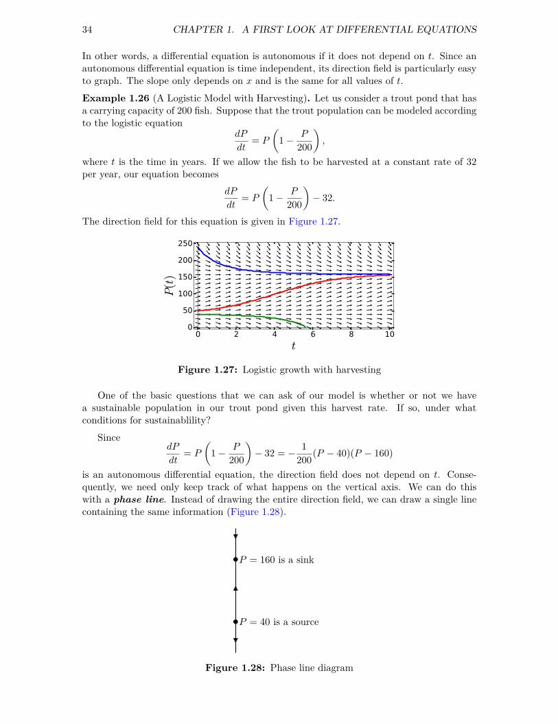
34 CHAPTER 1. A FIRST LOOK AT DIFFERENTIAL EQUATIONS
In other words, a differential equation is autonomous if it does not depend on t. Since anautonomous differential equation is time independent, its direction field is particularly easyto graph. The slope only depends on x and is the same for all values of t.Example 1.26 (A Logistic Model with Harvesting). Let us consider a trout pond that hasa carrying capacity of 200 fish. Suppose that the trout population can be modeled accordingto the logistic equation
dP
dt= P
(1− P
200
),
where t is the time in years. If we allow the fish to be harvested at a constant rate of 32per year, our equation becomes
dP
dt= P
(1− P
200
)− 32.
The direction field for this equation is given in Figure 1.27.
0 2 4 6 8 10
t
0
50
100
150
200
250
P(t
)
Figure 1.27: Logistic growth with harvesting
One of the basic questions that we can ask of our model is whether or not we havea sustainable population in our trout pond given this harvest rate. If so, under whatconditions for sustainablility?
SincedP
dt= P
(1− P
200
)− 32 = − 1
200(P − 40)(P − 160)
is an autonomous differential equation, the direction field does not depend on t. Conse-quently, we need only keep track of what happens on the vertical axis. We can do thiswith a phase line. Instead of drawing the entire direction field, we can draw a single linecontaining the same information (Figure 1.28).
P = 160 is a sink
P = 40 is a source
Figure 1.28: Phase line diagram

1.3. GEOMETRIC AND QUANTITATIVE ANALYSIS 35
Notice that dP/dt = 0 when P = 40 or P = 160. Thus, the two constant solutionsP (t) = 40 and P (t) = 160 are the same for all values of the independent variable t. We saythat such a solution is an equilibrium solution. Equilibrium solutions graph as horizontallines on the direction field. We can identify equilibrium solutions by setting the derivative ofthe function equal to zero. On our phase line we will represent these solutions as equilibriumpoints. For values of P between 40 and 160, we know that dP/dt > 0. Thus, any solutioncurve must be increasing. We denote this property on the phase line by drawing an upwardpointing arrow. On the other hand, we know that dP/dt < 0 when P < 40 or P > 160.In this case any solution curve will be decreasing, and we will indicate this by a downwardpointing arrow.
Let y′ = f(y) and suppose that y = y0 is an equilibrium solution. We say this solutionis a sink if for any solution y(t) with initial condition sufficiently close to y0, we have
limt→∞
y(t) = y0.
We say that an equilibrium point is a source if all solutions that start sufficiently close toy0 tend toward y0 as t→ −∞. An equilibrium solution that is neither a sink or a source iscalled a node (Figure 1.28). When P = 40, we have a source, and when P = 160, we havea sink
An equilibrium solution is stable if a small change in the initial conditions gives a solu-tion which tends toward the equilibrium as the independent variable tends towards positiveinfinity. An equilibrium solution is unstable if a small change in the initial conditions givesa solution which veers away from the equilibrium as the independent variable tends towardspositive infinity.
Consider the differential equation
dy
dt= y4 − 4y2 = y2(y + 2)(y − 2). (1.8)
The graph of f(y) = y4 − 4y2 is given in Figure 1.29. If y = −2, we have a sink. If y = 2,we have a source. Finally, if y = 0, we have a node.
-3 -2 -1 1 2 3y
-4
-2
2
4
6
dy/dt
Figure 1.29: Sinks, sources, and nodes
It is easy to generate a phase line diagram for equation (1.8) from the graph of f(y) =y2(y + 2)(y − 2) (Figure 1.29). If the graph is above the y-axis, then y is increasing. If thegraph is below the y-axis, then y is decreasing. Therefore, the phase line is easy to sketch(Figure 1.30).

36 CHAPTER 1. A FIRST LOOK AT DIFFERENTIAL EQUATIONS
y = 0 is a node
y = 2 is a source
y = −2 is a sink
Figure 1.30: Phase line diagram for y′ = y2(y + 2)(y − 2)
One of the reasons why autonomous equations are so important is Taylor’s theorem,which tells us that any function f(x) can be approximated near a point x0 by an nth degreepolynomial,
f(x) ≈ f(x0) + f ′(x0)(x− x0) +f ′′(x0)
2!(x− x0)
2 + · · ·+ f (n)(x0)
n!(x− x0)
n
near x0. For example, ifdx
dt= f(x) = cos(x2 + π)
with x(0) = x0, then we may approximate this initial value problem near x0 with
dx
dt= f(x0) + f ′(x0)(x− x0) = cos(x20 + π) + 2x0 sin(x20 + π)(x− x0)
x(0) = x0.
Of course, this strategy might not work very well if f(x0) = cos(x20 + π) = 0 or f ′(x0) =2x0 sin(x20 + π) = 0.
1.3.6 Important Lessons
• Direction fields and phase lines are a useful way of analyzing a differential equationfrom a geometric point of view, especially since not all differential equations can besolved analytically.
• An autonomous equation is a differential equation of the form y′ = f(y). We can usea phase line to analyze autonomous differential equations.
• Equilibrium solutions to a differential equation y′ = f(y) are those solutions givenby f(y) = 0 for all y. In this case, any solution must be constant. We can classifyequilibrium solutions according to whether they are stable or unstable. In particular,an equilibrium solution is either a sink, source, or node.

1.3. GEOMETRIC AND QUANTITATIVE ANALYSIS 37
1.3.7 Exercises1. Find all of the equilibrium solutions for each of the following differential equations.Use Sage to graph the direction field of each equation and then superimpose a plot of theequilibrium solution(s) on the direction field. Classify each equilibrium solution as a sink,a source, or a node.(a) y′ = 2y(1− y)
(b) dP
dt= 0.1P (P − 100)
(c) dx
dt= (2− x) cosx
(d) dy
dx= (2− y) cosx
2. Consider the differential equation y′ = f(y), where the graph of f(y) is given below.Identify any equilibrium solutions and classify each equilibrium solution as a sink, source,or node.
3. What happens if we increase the harvest rate to 100 in Example Example 1.26.? Whatshould be our strategy to maintain a viable population in the trout pond?
1.3.8 Sage—Plotting Direction Fields and SolutionsPlotting direction fields
If we wish to plot a direction field for a differential equation, we can use the commandplot_slope_field. Let us plot the direction field for the equation y′ = y2/2− t.
t, y = var( 't,y ' )f(t, y) = y^2/2 - tv = plot_slope_field(f, (t,-1,5), (y,-5,10), headaxislength =3,
headlength =3, axes_labels =[ ' $t$ ' , ' $y(t)$ ' ])v
There are a few extra commands to specify the size of the arrows in the plot and to labelthe axes. Try changing or omitting these commands and see what happens.
t, y = var( 't,y ' )f(t, y) = y^2/2 - tv = plot_slope_field(f, (t,-1,5), (y,-5,10), headaxislength =3,
headlength =3, axes_labels =[ ' $t$ ' , ' $y(t)$ ' ])v
For more examples and options, see http://doc.sagemath.org/html/en/reference/plotting/
sage/plot/plot_field.html
Plotting solutions
Now let us find a numerical solution to the equation using the command desolve_rk4. Thisis a fourth-order Runge-Kutta method, and returns a numerical solution (a table of values).Here, we must supply the dependent variable and initial conditions.
t, y = var( 't,y ' )f(t, y) = y^2/2 - t

38 CHAPTER 1. A FIRST LOOK AT DIFFERENTIAL EQUATIONS
p = desolve_rk4(f, y, ics=[-1,0], ivar=t, output= ' plot ' ,end_points =[-1,5], thickness =2)
p
Of course, we can combine the two plots.t, y = var( 't,y ' )f(t, y) = y^2/2 - tp = plot_slope_field(f, (t,-1,5), (y,-5,10), headaxislength =3,
headlength =3, axes_labels =[ ' $t$ ' , ' $y(t)$ ' ], fontsize =12)p += desolve_rk4(f, y, ics=[-1,0], ivar=t, output= ' plot ' ,
end_points =[-1,5], thickness =2)p
There are many other commands and packages to solve ordinary differential equationsusing Sage. For more information, see http://www.sagemath.org/doc/reference/calculus/
sage/calculus/desolvers.html. Below is an empty Sage cell, where you can practice.
Sage Exercises
1. Suppose that the population of a trout pond can be accurately modeled by the logisticequation
dp
dt= 0.4p
(1− p
500
).
At time t = 30, a disease is introduced into the population that kills 10% of the populationper year. To see how the disease affects the fish population, we will change our originalmodel to the folllowing:
dp
dt=
0.4p(1− p
500
)for 0 ≤ t < 30;
0.4p(1− p
500
)− 0.1p for t > 30.
(a) Plot the direction field for this equation using Sage.(b) Plot the graphs of two or three representative solutions to this equation on the direction
field.(c) Find formulas for the solutions of this equation for initial conditions p(0) = 30.(d) Give a qualitative description of how the disease affects the population.
1.4 Analyzing Equations NumericallyJust as numerical algorithms are useful when finding the roots of polynomials, numericalmethods will prove very useful in our study of ordinary differential equations. Consider thepolynomial f(x) = x2−2. We do not need a numerical algorithm to see that the roots of thispolynomial are x =
√2 and x = −
√2. However, a numerical method such as the Newton-
Raphson Algorithm is very useful for approximating√2 as a decimal.6 Similarly, it may be
easier to generate a numerical solution for differential equations if our goal is simply to plota solution. In addition, there will be differential equations for which it is impossible to finda solution in terms of elementary functions such as polynomials, trigonometric functions,and exponential functions.
6See any calculus text for a description of the Newton-Raphson Algorithm.

1.4. ANALYZING EQUATIONS NUMERICALLY 39
1.4.1 Euler’s MethodSuppose that we wish to solve the initial value problem
y′ = f(t, y) = y + t, (1.9)y(0) = 1. (1.10)
The equation y′ = y + t is not separable, which currently is the only analytic technique atour disposal. However, we can try to find a numerical approximation for the solution. Anumerical approximation is simply a table (possibly very large) of t and y values.
We will attempt to find a numerical solution for (1.9)–(1.10) on the interval [0, 1]. Evenwith the use of a computer, we cannot approximate the solution at every single point on aninterval. For the initial value problem
y′ = f(t, y)
y(t0) = y0,
we might be able to find approximations at a = t0, t1, t2, . . . , tN = b in [a, b] at best. If wechoose t1, t2, . . . , tN to be equally spaced on [a, b], we can write
tk = t0 + kh,
where h = 1/N and k = 1, 2, . . . , N . We say that h is the step size for our approximation.Given an approximation Yk for the solution yk = y(tk), the question is how to find an
approximate solution Yk+1 at tk+1. To generate the second approximation, we will constructa tangent line to the solution at y(t0) = y0. If we use slope of the solution curve at t0, then
y′(t0) = f(y0, t0).
Making use of the fact that
y(t0 + h)− y(t0)
h≈ y′(t0, y(t0)) = y′(t0, y0)
or equivalentlyy(t0 + h) = y(t1) ≈ y(t0) + hy′(t0, y0),
the estimate for our solution at t1 = t0 + h is
Y1 = Y0 + hf(t0, Y0).
Similarly, the approximation at t2 = t0 + 2h will be
Y2 = Y1 + hf(t1, Y1).
Our general algorithm isYk+1 = Yk + hf(tk, Yk).
The idea is to compute tangent lines at each step and use this information to get our nextapproximation.
The algorithm that we have described is known as Euler’s method. Let us estimate asolution to (1.9)–(1.10) on the interval [0, 1] with step size h = 0.1. Since y(0) = 1, We canmake our first approximation exact,
Y0 = y(0) = 1.

40 CHAPTER 1. A FIRST LOOK AT DIFFERENTIAL EQUATIONS
To generate the second approximation, we will construct a tangent line to the solution aty(0) = 1. If we use slope of the solution curve at t0 = 0,
y′(0) = f(y(0), 0) = y(0) + 0 = 1 + 0 = 1,
and make use of the fact that
y(h)− y(0)
h≈ y′(0, y(0)) or y(h) ≈ y(0) + y′(0, y(0)),
the estimate for our solution at t = 0.1 is
Y1 = Y0 + hf(t0, Y0)
= Y0 + h[Y0 + t0]
= 1 + (0.1)[1 + 0]
= 1.1000.
Similarly, the approximation at t = 0.2 will be
Y2 = Y1 + hf(t1, Y1)
= Y1 + h[Y1 + t1]
= 1.1000 + (0.1)[1.1000 + 0.1]
= 1.2200.
Our general algorithm is
Yk+1 = Yk + hf(tk, Yk) = Yk + h[Yk + tk] = (1.1)Yk + (0.01)k.
The initial value problem (1.9)–(1.10) is, in fact, solvable analytically with solutiony(t) = 2et − t− 1. We can compare our approximation to the exact solution in Table 1.31.We can also see graphs of the approximate and exact solutions in Figure 1.32. Notice thatthe error grows as we get further away from our initial value. In fact, the graph of theapproximation for h = 0.001 is obscured by the graph of the exact solution. In addition, asmaller step size gives us a more accurate approximation (Table 1.33).
k tk Yk yk |yk − Yk| Percent Error0 0.0 1.0000 1.0000 0.0000 0.00%1 0.1 1.1000 1.1103 0.0103 0.93%2 0.2 1.2200 1.2428 0.0228 1.84%3 0.3 1.3620 1.3997 0.0377 2.69%4 0.4 1.5282 1.5836 0.0554 3.50%5 0.5 1.7210 1.7974 0.0764 4.25%6 0.6 1.9431 2.0442 0.1011 4.95%10 1.0 3.1875 3.4366 0.2491 7.25%
Table 1.31: Euler’s approximation for y′ = y + t

1.4. ANALYZING EQUATIONS NUMERICALLY 41
0 0.2 0.4 0.6 0.8 1
1
1.5
2
2.5
3
3.5 h= 0. 1h= 0. 02h= 0. 001yexact
Figure 1.32: Euler’s approximation for y′ = y + t
tk h = 0.1 h = 0.02 h = 0.001 Exact Solution0.1 1.1000 1.1082 1.1102 1.11030.2 1.2200 1.2380 1.2426 1.24280.3 1.3620 1.3917 1.3993 1.39970.4 1.5282 1.5719 1.5831 1.58360.5 1.7210 1.7812 1.7966 1.79740.6 1.9431 2.0227 2.0431 2.04420.7 2.1974 2.2998 2.3261 2.32750.8 2.4872 2.6161 2.6493 2.65110.9 2.8159 2.9757 3.0170 3.10921.0 3.1875 3.3832 3.4238 3.4366
Table 1.33: Step sizes for Euler’s approximation
1.4.2 Finding an Error Bound
To fully understand Euler’s method, we will need to recall Taylor’s theorem from calculus.
Theorem 1.34. If x > x0, then
f(x) = f(x0) + f ′(x0)(x− x0) +f ′′(x0)
2!(x− x0)
2 + · · ·+ f (n)(ξ)
n!(x− x0)
n,
where ξ ∈ (x0, x).
Given the initial value problem
y′ = f(t, y),
y0 = y(t0),
choose t1, t2, . . . , tN to be equally spaced on [t0, a], we can write
tk = t0 + kh,

42 CHAPTER 1. A FIRST LOOK AT DIFFERENTIAL EQUATIONS
where h = (a− t0)/N and k = 1, 2, . . . , N . Taylor’s Theorem tells us that
y(tk+1) = y(tk + h) = y(tk) + y′(tk)h+y′′(tk)
2!h2 + · · · .
If we know the values of y and its derivatives at tk, then we can determine the value of yat tk+1.
The simplest approximation can be obtained by taking the first two terms of the Taylorseries. That is, we will use a linear approximation,
yk+1 = y(tk+1) ≈ y(tk) + y′(tk)h = y(tk) + f(tk, yk)h.
This gives us Euler’s method,
Y0 = y(t0)
Y1 = Y0 + hf(t0, Y0)
Y2 = Y1 + hf(t1, Y1)
...Yk+1 = Yk + hf(tk, Yk).
The terms that we are omitting, all contain powers of h of at least degree two. If h is small,then hn for n = 2, 3, . . . will be very small and these terms will not matter much.
We can actually estimate the error incurred by Euler’s method if we make use of Taylor’sTheorem.
Theorem 1.35. Let y be the unique solution to the initial value problem
y′ = f(t, y),
y(a) = α,
where t ∈ [a, b]. Suppose that f is continuous and there exists a constant L > 0 such that
|f(t, y1)− f(t, y2)| ≤ L|y1 − y2|,
whenever (t, y1) and (t, y2) are in D = [a, b]× R. Also assume that there exists an M suchthat
|y′′(t)| ≤M
for all t ∈ [a, b]. If Y0, . . . , YN are the approximations generated by Euler’s method for somepositive integer N , then
|y(ti)− Yi| ≤hM
2L[eL(ti−a) − 1].
The condition that there exists a constant L > 0 such that
|f(t, y1)− f(t, y2)| ≤ L|y1 − y2|,
whenever (t, y1) and (t, y2) are in D = [a, b]×R is called a Lipschitz condition. Many ofthe functions that we will consider satisfy such a condition. If the condition is satisfied, wecan usually say a great deal about the function.

1.4. ANALYZING EQUATIONS NUMERICALLY 43
k tk Yk yk = y(tk) |yk − Yk| Estimated Error0 0.0 1.0000 1.0000 0.0000 0.00001 0.1 1.1000 1.1103 0.0103 0.02862 0.2 1.2200 1.2428 0.0228 0.06023 0.3 1.3620 1.3997 0.0377 0.09514 0.4 1.5282 1.5836 0.0554 0.13375 0.5 1.7210 1.7974 0.0764 0.17636 0.6 1.9431 2.0442 0.1011 0.22357 0.7 2.1974 2.3275 0.1301 0.27568 0.8 2.4872 2.6511 0.1639 0.33319 0.9 2.8159 3.1092 0.2033 0.396810 1.0 3.1875 3.4366 0.2491 0.4671
Table 1.36: Error bound and actual error
We can now compare the estimated error from our theorem to the actual error of ourexample. We first need to determine M and L. Since
|f(t, y1)− f(t, y2)| = |(y1 + t)− (y2 + t)| = |y1 − y2|,
we can take L to be one. Since y′′ = 2et, we can bound y′′ on the interval [0, 1] by M = 2e.Thus, we can bound the error by
|y(ti)− Yi| ≤hM
2L[eL(ti−a) − 1] = 0.1e(eti − 1)
for h = 0.1. Our results are in Table 1.36.
1.4.3 Improving Euler’s Method
If we wish to improve upon Euler’s method, we could add more terms of Taylor series.For example, we can obtain a more accurate approximation by using a quadratic Taylorpolynomial,
y(t1) ≈ y0 + f(t0, y0)h+y′′(t0)
2h2.
However, we need to know y′′(t0) in order to use this approximation. Using the chain rulefrom multivariable calculus, we can differentiate both sides of y′ = f(t, y) to obtain
y′′ =∂f
∂t
dt
dt+∂f
∂y
dy
dt= ft + ffy.
Thus, our approximation becomes
y(t1) ≈ y0 + f(t0, y0)h+1
2(ft(t0, y0) + f(t0, y0)fy(t0, y0))h
2.
The problem is that some preliminary analytic work must be done. That is, before wecan write a program to compute our solution, we must find ∂f/∂t and ∂f/∂y, althoughthis is less of a problem with the availability of computer algebra systems such as Sage.
Around 1900, two German mathematicians, Carle Runge and Martin Kutta, indepen-dently invented several numerical algorithms to solve differential equations. These methods,

44 CHAPTER 1. A FIRST LOOK AT DIFFERENTIAL EQUATIONS
known as Runge-Kutta methods, estimate the higher-order terms of the Taylor series tofind an approximation that does not depend on computing derivatives of f(t, y).
If we consider the initial value problem
y′ = f(t, y),
y(t0) = y0,
theny(t1) = y(t0) +
∫ t1
t0
f(s, y(s)) ds
ory1 − y0 = y(t1)− y(t0) =
∫ t1
t0
f(s, y(s)) ds (1.11)
by the Fundamental Theorem of Calculus. In Euler’s method, we approximate the right-hand side of (1.11) by
y1 − y0 = f(t0, y0)h.
In terms of the definite integral, this is simply a left-hand sum. In the improved Euler’smethod or the second-order Runge-Kutta method we will estimate the right-hand sideof (1.11) using the trapezoid rule from calculus,
y(t1)− y(t0) =
∫ t1
t0
f(s, y(s)) ds
≈ (f(t0, y0) + f(t1, y1))h
2.
Thus, our algorithm becomes
y1 = y0 + (f(t0, y0) + f(t1, y1))h
2. (1.12)
However, we have a problem since y1 appears in the right-hand side of our approximation.To get around this difficulty, we will replace y1 in the right-hand side of (1.12) with theEuler approximation for y1. Thus,
y1 = y0 + (f(t0, y0) + f(t1, y0 + f(t0, y0)h))h
2.
To understand that the second-order Runge-Kutta method is actually an improvementover the traditional Euler’s method, we will need to use the Taylor approximation for afunction of two variables. Let us assume that f(x, y) is defined on some rectangle and thatall of the derivatives of f are continuously differentiable. Then
f(x+ h, y + k) = f(x, y) + h∂
∂xf(x, y) + k
∂
∂yf(x, y)
+1
2!
(h2
∂2
∂2xf(x, y) + hk
∂2
∂x∂yf(x, y) + k2
∂2
∂2yf(x, y)
)+
1
3!
(h3
∂3
∂3xf(x, y) + 3h2k
∂3
∂2x∂yf(x, y)
+ hk2∂3
∂x∂2yf(x, y) + k3
∂3
∂3yf(x, y)
)+ · · · .

1.4. ANALYZING EQUATIONS NUMERICALLY 45
As in the case of the single variable Taylor series, we can write a Taylor polynomial if theTaylor series is truncated,
f(x+ h, y + k) =
N∑n=0
1
n!
(h∂
∂x+ k
∂
∂y
)n
f(x, y)
+1
(N + 1)!
(h∂
∂x+ k
∂
∂y
)N+1
f(x, y),
where the second term is the remainder term and (x, y) lies on the line segment joining(x, y) and (x+ h, y + k).
In the Improved Euler’s Method, we adopt a formula
y(t+ h) = y(t) + w1F1 + w2F2,
where
F1 = hf(t, y)
F2 = hf(t+ αh, y + βF1).
That is,y(t+ h) = y(t) + w1hf(t, y) + w2hf(t+ αh, y + βhf(t, y)). (1.13)
The idea is to choose the constants w1, w2, α, and β as accurately as possible in order toduplicate as many terms as possible in the Taylor series
y(t+ h) = y(t) + hy′(t) +h2
2!y′′(t) +
h3
3!y′′(t) + · · · . (1.14)
We can make equations (1.13) and (1.14) agree if we choose w1 = 1 and w2 = 0. Sincey′ = f , we obtain Euler’s method.
If we are more careful about choosing our parameters, we can obtain agreement upthrough the h2 term. If we use the two variable Taylor series to expand f(t+αh, y+ βhf),we have
f(t+ αh, y + βhf) = f + αhft + βhffy +O(h2),
where O(h2) means that of the subsequent terms have a factor of hn with n ≥ 2. Using thisexpression, we obtain a new form for (1.13),
y(t+ h) = y(t) + (w1 + w2)hf + αw2h2ft + βw2h
2ffy +O(h3). (1.15)
Since y′′ = ft + fyf by the chain rule, we can rewrite (1.14) as
y(t+ h) = y(t) + hf +h2
2!(ft + ffy) +O(h3). (1.16)
We can make equations (1.15) and (1.16) agree up through the quadratic terms if we requirethat
w1 + w2 = 1,
αw2 =1
2,
βw2 =1
2.

46 CHAPTER 1. A FIRST LOOK AT DIFFERENTIAL EQUATIONS
If we choose α = β = 1 and w1 = w2 = 1/2, these equations are satisfied and we obtain theimproved Euler’s method
y(t+ h) = y(t) +h
2f(t, h) +
h
2f(t+ h, y + hf(t, y)).
The improved Euler’s method or the second-order Runge-Kutta method is a more so-phisticated algorithm that is less prone to error due to the step size h. Euler’s method isbased on truncating the Taylor series after the linear term. Since
y(t+ h) = y(t) + hy′(t) +O(h2),
we know that the error depends on h. On the other hand, the error for the improved Euler’smethod depends on h2, since
y(t+ h) = y(t) + hy′(t) +h2
2!y′′(t) +O(h3).
If we use Simpson’s rule to estimate the integral in
y(t1)− y(t0) =
∫ t1
t0
f(s, y(s)) ds
we can improve our accuracy up to h4. The idea is exactly the same, but the algebra becomemuch more tedious. This method is known as the Runge-Kutta method of order 4 and isgiven by
y(t+ h) = y(t) +1
6(F1 + 2F2 + 2F3 + F4),
where
F1 = hf(t, y)
F2 = hf
(t+
1
2h, y +
1
2F1
)F3 = hf
(t+
1
2h, y +
1
2F2
)F4 = hf(t+ h, y + F3).
1.4.4 Important Lessons
• We can use Euler’s method to find an approximate solution to the initial value problem
y′ = f(t, y),
y(a) = α
on an interval [a, b]. If we wish to find approximations at N equally spaced pointst1, . . . , tN , where h = (b− a)/N and ti = a+ ih, our approximations should be
Y0 = α,
Y1 = Y0 + hf(α, Y0),
Y2 = Y1 + hf(t1, Y1, )
...Yk+1 = Yk + hf(tk, Yk),
YN = YN−1 + hf(tN−1, YN−1).

1.4. ANALYZING EQUATIONS NUMERICALLY 47
• Taylor’s Theorem theorem is a very useful tool for studying differential equations. Ifx > x0, then
f(x) = f(x0) + f ′(x0)(x− x0) +f ′′(x0)
2!(x− x0)
2 + · · ·+ f (n)(ξ)
n!(x− x0)
n,
where ξ ∈ (x0, x).
• Error analysis rate of convergence is very important for any numerical algorithm. Ourapproximation is more accurate for smaller values of h. Under reasonable conditionswe can also bound the error by
|y(ti)− Yi| ≤hM
2L[eL(ti−a) − 1],
where y is the unique solution to the initial value problem
y′ = f(t, y),
y(a) = α.
• The condition that there exists a constant L > 0 such that
|f(t, y1)− f(t, y2)| ≤ L|y1 − y2|,
whenever (t, y1) and (t, y2) are in D = [a, b]× R is called a Lipschitz condition.
• Using Taylor series, we can develop better numerical algorithms to compute solutionsof differential equations. The Runge-Kutta methods are an important class of thesealgorithms.
• The improved Euler’s method is given by
y(t+ h) = y(t) +h
2f(t, h) +
h
2f(t+ h, y + hf(t, y))
with the error bound depending on h2.
• The Runge-Kutta method of order 4 is given by
y(t+ h) = y(t) +1
6(F1 + 2F2 + 2F3 + F4),
where
F1 = hf(t, y)
F2 = hf
(t+
1
2h, y +
1
2F1
)F3 = hf
(t+
1
2h, y +
1
2F2
)F4 = hf(t+ h, y + F3)
with the error bound depending on h4.

48 CHAPTER 1. A FIRST LOOK AT DIFFERENTIAL EQUATIONS
1.4.5 Exercises1. Consider the differential equation
dy
dt= 3y − 1
with initial value y(0) = 2.(a) Find the exact solution of the initial value problem.(b) Use Euler’s method with step size h = 0.5 to approximate the solution to the initial
value problem on the interval [0, 2] Your solution should include a table of approximatevalues of the dependent variable as well as the exact values of the dependent variable.Make sure that your approximations are accurate to four decimal places.
(c) Sketch the graph of the approximate and exact solutions.(d) Use the error bound theorem (Theorem Theorem 1.35) to estimate the error at each
approximation. Your solution should include a table of approximate values of thedependent variable the exact values of the dependent variable, the error estimates, andthe actual error. Make sure that your approximations are accurate to four decimalplaces.
2. In this series of exercises, we will prove the error bound theorem for Euler’s method(Theorem Theorem 1.35).(a) Use Taylor’s Theorem to show that for all x ≥ −1 and any positive m,
0 ≤ (1 + x)m ≤ emx.
(b) Use part (1) and geometric series to prove the following statement: If s and t arepositive real numbers, and aiki=0 is a sequence satisfying
a0 ≥ − t
sai+1 ≤ (1 + s)ai + t, for i = 0, 1, 2, . . . , k,
thenai+1 ≤ e(i+1)s
(t
s+ a0
)− t
s.
(c) When i = 0, y(t0) = Y0 = α and the theorem is true. Use Euler’s method and Taylor’sTheorem to show that
|yi+1 − Yi+1| ≤ |yi − Yi|+ h|f(ti, yi)− f(ti, Yi)|+h2
2|y′′(ξi)|
where ξi ∈ (ti, ti+1) and yk = y(tk).(d) Show that
|yi+1 − Yi+1| ≤ |yi − Yi|(1 + hL) +Mh2
2.
(e) Let aj = |yj − Yj | for j = 0, 1, . . . , N , s = hL, and t = Mh2/2 and apply part (2) toshow
|yi+1 − Yi+1| ≤ e(1+i)hL
(|y0 − Y0|+
Mh2
2hL
)− Mh2
2hL.
and derive that|yi+1 − Yi+1| ≤
Mh
2L
(e(ti+1−a)L − 1
)for each i = 0, 1, . . . , N − 1.

1.4. ANALYZING EQUATIONS NUMERICALLY 49
Hint. Hints for part (2):• For fixed i show that
ai+1 ≤ (1 + s)ai + t
≤ (1 + s)[(1 + s)ai−1 + t] + t
≤ (1 + s)(1 + s)[(1 + s)ai−2 + t] + t+ t
...≤ (1 + s)i+1a0 + [1 + (1 + s) + (1 + s)2 + · · ·+ (1 + s)i]t.
• Now use a geometric sum to show that
ai+1 ≤ (1 + s)i+1a0 +t
s[(1 + s)i+1 − 1] = (1 + s)i+1
(t
s+ a0
)− t
s.
• Apply part (1) to derive
ai+1 ≤ e(i+1)s
(t
s+ a0
)− t
s.
1.4.6 Project—Numerical Routines for solving ODEsNot all differential equations can be solved using algebra and calculus even if we are veryclever. If we encounter an equation that we cannot solve or use Sage to solve, we mustresort to numerical algorithms like Euler’s method or one of the Runge-Kutta methods,which are best implemented using a computer. Fortunately, Sage has some very goodnumerical solvers. Sage will need to know the following to solve a differential equation:
• An abstract function
• A differential equation, including an initial condition
• A Sage command to solve the equation.
Suppose we wish to solve the initial value problem dy/dx = x + y, y(0) = 1. We canuse Sage to find an algebraic solution.y = function( ' y ' )(x)de = diff(y,x) == x + yh = desolve(de , y, ics = [0,1])show(h)plot(h, x, 0, 5)
We can also use Euler’s method to find a solution for our initial value problem.x,y = PolynomialRing(RR, 2, "xy").gens() #declare x, y as generators
of a polynomial ringeulers_method(x + y, 0,1, 0.5, 5)
The syntax of eulers_method for the inital value problem
y = f(x, y)
f(x0) = y0
with step size h on the interval [x0, x1] is eulers_method(f, x0, y0, h, x1) Notice thatwe obtained a table of values. However, we can use the line command from Sage to plotthe values (x, y).

50 CHAPTER 1. A FIRST LOOK AT DIFFERENTIAL EQUATIONS
x,y = PolynomialRing(RR, 2, "xy").gens()pts = eulers_method(x + y, 0, 1, 1/2, 4.5, algorithm="none")p = list_plot(pts , color="red")p += line(pts)p
As we pointed out, eulers_method is not very sophisticated. We have to use a very smallstep size to get good accuracy, and the method can generate errors if we are not careful.Fortunately, Sage has much better algorithms for solving initial value problems. One suchalgorithm is desolve_rk4, which implements the fourth order Runge-Kutta method.
x,y = var( ' xy ' )desolve_rk4(x + y, y, ics=[0, 1], end_points = 5, step = 0.5)
Again, we just get a list of points. However, desolve_rk4 has some nice built-in graphingutilities.
x,y = var( ' xy ' )p = desolve_rk4(x + y, y, ics = [0,1], ivar = x, output =
' slope_field ' , end_points = [0, 5], thickness = 2, color = ' red ' )p
Write the Sage commands to compare the graphs obtained using eulers_method and des-olve with the exact solution.
Not only is desolve_rk4 more accurate, it is much easier to use. For more information, seehttp://www.sagemath.org/doc/reference/calculus/sage/calculus/desolvers.html.
1.5 First-Order Linear EquationsA first-order differential equation is an equation of the form
dx
dt+ p(t)x = q(t). (1.17)
This equation will not be separable if p(t) is not a constant. We shall have to find a newapproach to solving such an equation. We could, of course, use a numerical algorithmto solve (1.17); however, we can always find an algebraic solution to a first-order lineardifferential equation. Moreover, the fact that we can obtain such a solution analyticallywill prove very useful when we investigate more complicated equations and systems ofequations.
1.5.1 Mine TailingsIn any mining operation, tailings are what is left after everything of value has been extracted.For example, in a hard rock mining operation, ore is often pulverized and then processedusing chemicals to extract certain minerals of value. Soft rock mining operations such as coalmining or extracting oil from tar sands might use solvents or water to extract any commodityof value. The material that is left over after the minerals, coal, or oil is extracted can oftenpresent huge environmental challenges. There are different ways of processing mine tailings,but one way is to store them in a pond, especially if water is used in the mining operation.

1.5. FIRST-ORDER LINEAR EQUATIONS 51
This method allows any particles that are suspended in the water to settle to the bottomof the pond. The water can then be treated and recycled.
Suppose that we have a gold mining operation and we are storing our tailings in a pondthat has an initial volume of 20,000 cubic meters. When we begin our operation, the tailingspond is filled with clean water. The pond has a stream flowing into it, and water is alsopumped out of the pond. Chemicals are used in processing gold ore. These chemicals suchas sodium cyanide can be highly poisonous and dangerous to the environment, and thewater must be treated before it is released into the watershed. Suppose that 1000 cubicmeters per day flow into the pond from stream and 1000 cubic meters are pumped fromthe pond each day to be processed and recycled. Thus, the water level of the pond remainsconstant.
At time t = 0, the water from stream becomes contaminated with chemicals from themining operation, say at a rate of 5 kilograms of chemicals per 1000 cubic meters. We willassume that water in our tailings pond is well mixed so that the concentration of chemicalsthrough out the pond is fairly uniform. In addition, any particulate matter pumped intothe pond from the stream settles to the bottom of the pond at a rate of 50 cubic metersper day. Thus, the volume of our tailings pond is reduced by 50 cubic meters each day, andour tailings pond will become full after 400 days of operation. We shall assume that theparticulate matter and the chemicals are included in the 1000 cubic meters that flow intothe pond from the stream each day.
We wish to find a differential equation that will model the amount of chemicals in thetailings pond at any particular time. Let x(t) be the amount of chemicals in the pond attime t. Then dx/dt is the difference between the rate at which the chemicals are enteringthe pond and the rate at which the chemicals leave the pond.
dx
dt= rate in − rate out.
Since water flows into the pond from the stream at a rate of 1000 cubic meters per day,the rate at which the chemicals enter the pond is 5 kilograms per day. On the other hand,the rate at which the chemicals leave the pond will depend on the amount of chemicals inthe pond at time t. The volume of the pond is decreasing due to sediment, and at timet it is V (t) = 20000 − 50t. Thus, the concentration of chemicals in the pond at time t isx/(20000 − 50t), and the rate at which the chemicals are flowing out of the pond to berecycled is
1000
(x
20000− 50t
)=
20x
400− t.
Hence, the differential equation that models the amount of chemical in the tailings pond attime t is
dx
dt= 5− 20x
400− t. (1.18)
Of course, we will have to cease mining operations once the pond is full, since there willonly be water in the pond if V (t) = 20000− 50t ≥ 0; that is, when 0 ≤ t < 400.
Notice that equation (1.18) is not autonomous. In fact, it is not even separable. Wewill have to use a different approach to find a solution. First, we will rewrite the equationin the form
dx
dt+
20
400− tx = 5.
If we multiply both sides of this equation by (400− t)−20, we obtain
(400− t)−20dx
dt+ 20(400− t)−21x = 5(400− t)−20. (1.19)

52 CHAPTER 1. A FIRST LOOK AT DIFFERENTIAL EQUATIONS
We now make the crucial observation that the product rule applies to the lefthand side ofour equation,
(400− t)−20dx
dt+ 20(400− t)−21x =
d
dt
((400− t)−20x
).
Thus, equation (1.19) becomes
d
dt
((400− t)−20x
)= 5(400− t)−20.
Integrating both sides of this equation, we have
(400− t)−20x = 5
∫(400− t)−20 dt =
5(400− t)−19
19+ C,
where C is an arbitrary constant. Solving for x, we obtain
x(t) =5
19(400− t) + C(400− t)20.
Since x(0) = 0, we can quickly determine that C = −(5/19)400−19 and that the solution toour initial value problem is
x(t) =5
19(400− t)
[1−
(400− t
400
)19].
The graph of the solution to our differential equation (Figure 1.37) fits the situation. Ini-tially, there are no chemicals in the pond, but x(t) quickly increases. However, the amountof chemicals decreases as the pond begins to fill with sediment. Eventually, there are nochemicals at t = 400.
100 200 300 400t
20
40
60
80
x(t)
Figure 1.37: Chemical waste in a tailings pond

1.5. FIRST-ORDER LINEAR EQUATIONS 53
1.5.2 First-Order Linear EquationsThe differential equation
dx
dt+
20
400− tx = 5
is an example of a first-order linear differential equation. More specifically, a first-orderlinear differential equation is an equation that can be written in the form
dx
dt+ p(t)x = q(t).
Let us first show how to solve first-order linear equations when the coefficient functions areconstant. If
dx
dt+ px = q,
x(t0) = x0,
then we first multiply both sides of the equation by ept to obtain
eptdx
dt+ eptpx = qept.
The left-hand side of the equation is exact That is,
eptdx
dt+ eptpx =
d
dt
(x(t)ept
).
If we integrate both sides ofd
dt
(x(t)ept
)= qept,
thenx(t)ept =
q
pept + C.
If we apply the initial condition, we can determine C,
C =
(x0 −
q
p
)ept0 .
Thus, the solution that we seek is
x(t) =q
p+
(x0 −
q
p
)ep(t0−t).
Example 1.38. Suppose we wish to solve the initial value problemdx
dt− 2x = 3, (1.20)
x(0) = 1. (1.21)
Multiplying both sides of equation (1.20) by e−2t, we obtaind
dt
(e−2tx
)= e−2tdx
dt− 2e−2tx = 3e−2t.
Integrating both sides of this last equation, gives us the following
e−2tx = 3
∫e−2t dt+ C = −3
2e−2t + C.
Applying the initial condition x(0) = 1, we can conclude that C = 5/2, and
x(t) =5
2e2t − 3
2.

54 CHAPTER 1. A FIRST LOOK AT DIFFERENTIAL EQUATIONS
Example 1.39. Now let us solve a first-order linear differential equation where the coeffi-cients are not constant. Suppose that
y′ + 2xy = e−x2,
where y(0) = 1. We will multiply both sides of the equation by ex2 and use the product
rule to obtaind
dx
(ex
2y)= ex
2y′ + 2xex
2y = ex
2e−x2
= 1.
Integrating both sides, we getex
2y =
∫dx+ C.
Thus, the general solution isy = (x+ C)e−x2
.
Using the initial condition to solve for C, we find that C = 1 and
y = (x+ 1)e−x2.
We can use Sage to check our solution.
x = var( ' x ' )y = function( ' y ' )(x)de = diff(y, x) + 2*x*y == exp(-x^2)solution = desolve(de, y, ics = [0, 1])solution
(x + 1)*e^(-x^2)
Surprisingly, the strategy in Example 1.39 will always work. Suppose that
x′ + p(t)x = q(t). (1.22)
If we choose P (t) such that P ′(t) = p(t) and multiply both sides of the equation by eP (t),then (
eP (t)x)′
= eP (t)(x′(t) + p(t)x(t) = eP (t)q(t).
Integrating both sides,eP (t)x =
∫eP (t)q(t) dt+ C
orx =
1
eP (t)
(∫eP (t)q(t) dt+ C
).
The Fundamental Theorem of Calculus tells us that P (t) =∫p(t) dt. We say that
µ(t) = e∫p(t) dt = exp
(∫p(t) dt
)is an integrating factor for the differential equation (1.22).
Example 1.40. Consider the initial value problem
dy
dx− 2
xy = 2x2
y(−2) = 4.

1.5. FIRST-ORDER LINEAR EQUATIONS 55
Our integrating factor is
µ(x) = exp(−∫
2
xdx
)= e−2 lnx = elnx−2
= x−2.
Multiplying both of our differential equation by µ(x) = x−2, we obtain
x−2
(dy
dx− 2
xy
)= 2
ord
dx
(x−2y
)= x−2 dy
dx− 2x−3y = 2.
We can now integrate this equation to get
x−2y = 2x+ C.
The initial condition y(−2) = 4 allows us to find C = 5. Therefore, the solution to ourinitial value problem is
y = 2x3 + 5x2.
1.5.3 Mixing ModelsMany applications involve the mixing of two or more substances together. We can modelhow petroleum products are mixed together in a refinery, how various ingredients are mixedtogether in a brewery, or how greenhouse gases move across various layers of the earth’satmosphere.
Example 1.41. Suppose that a 100-gallon tank initially contains 50 gallons of salt watercontaining five pounds of salt. A brine mixture containing one pound of salt per gallonflows into the top of the tank at a rate of 5 gallons per minute. A well mixed solution leavesthe tank at rate of 4 gallons per minute. We wish to know how much salt is in the tank,when the tank is full.
To construct our model, we will let t be the time (measured in minutes) and set upa differential equation that will measure how fast the amount of salt at time t, x(t), ischanging. We have the initial condition x(0) = 5, and
dx
dt= amount of salt flowing in − amount of salt flowing out
= 5︸︷︷︸in flow
− 4x
V (t)︸ ︷︷ ︸out flow
,
where V (t) is the volume at time t. The expression x/V (t) is the amount of salt in onegallon at time t. We have V (t) = 50 + t, since the tank starts with 50 gallons and fivegallons are pumped into the tank per minute while four gallons leave the tank during thesame time interval. Thus, our differential equation becomes
dx
dt= 5− 4
50 + tx.
Our equation is linear since we can rewrite it as
dx
dt+
4
50 + tx = 5. (1.23)

56 CHAPTER 1. A FIRST LOOK AT DIFFERENTIAL EQUATIONS
An integrating factor for this differential equation is
µ(t) = exp(∫
4
50 + tdt
)= e4 ln(50+t) = (50 + t)4.
Therefore, if we multiply both sides of equation (1.23) by µ(t), we get
(50 + t)4dx
dt+ 4(t+ 50)3x = 5(50 + t)4.
We can now apply the product rule to obtain
d
dt[(50 + t)4x] = 5(50 + t)4.
Integrating both sides and simplifying gives us
x = t+ 50 +C
(t+ 50)4.
Our initial condition, x(0) = 5 tells us that C = 31, 250, 000 and
x(t) = t+ 50− 31250000
(t+ 50)4.
Thus, when the tank is full, t = 50 and the amount of salt in the tank is x(50) = 97.188pounds. We can use Sage to easily check the solution of our initial value problem.
t = var( ' t ' )x = function( ' x ' )(t)de = diff(x, t) + 4*x/(50 + t) == 5solution(t) = desolve(de, x, ics=[0, 5])solution (50).n(digits = 5)
97.188
1.5.4 Finance ModelsThere are a number of problems in finance that can be modeled using differential equations.Let P (t) be the balance of an account at time t and suppose that the account pays interestat a rate of r percent per year compounded continuously. Suppose that we also allowwithdrawals of W dollars per year. The net increase in the balance between times t andt+∆t can now be described as
P (t+∆t)− P (t) ≈ rP∆t−W∆t
Thus,P ′(t) = lim
∆t→0
P (t+∆t)− P (t)
∆t= rP −W.
We can solve the equationP ′ = rP −W
by multiplying both sides of the equation by the integrating factor
µ(t) = exp(−∫r dt
)= e−rt.

1.5. FIRST-ORDER LINEAR EQUATIONS 57
to obtaind
dt[e−rtP ] = −We−rt.
Integrating both sides of this equation, we have
e−rtP =W
re−rt + C
or
P =W
r+ Cert.
If we know the initial balance in the account, say P (0) = P0, we can determine C. That is,
P0 =W
r+ C
or
C = P0 −W
r.
Thus, the solution to our initial value problem is
P =W
r+
(P0 −
W
r
)ert.
Example 1.42. Suppose that your parents have established a money market account witha balance of $50,000 that they will use to help you pay for your college education. Theaccount receives an average annual interest of 4%. You estimate that your tuition, roomand board, and other college expenses to be $20,000 per year.
We model this financial situation with the differential equation
dP
dt= 0.04P − 20000
P (0) = 50000.
Rewriting the differential equation as dP/dt − 0.04P = −20000, our integrating factorbecomes µ(t) = e−0.04t, and
e−0.04tdP
dt− 0.04e−0.04tP =
d
dt[e−0.04tP ] = −20000e−0.04t.
Thus,
e−0.04tP =20000
0.04e−0.04t + C = 500000e−0.04t + C.
The solution to this initial-value problem is
P (t) =20000
0.04+
(50000− 20000
0, 04
)e0.04t = 500000− 450000e0.04t.
Your parents have been quite generous but have told you that you must be responsiblefor the balance of the cost of your education.

58 CHAPTER 1. A FIRST LOOK AT DIFFERENTIAL EQUATIONS
1.5.5 Existence and Uniqueness of SolutionsSeveral questions about the existence and uniqueness of solutions to first-order linear dif-ferential equations now arise.
• Does an initial-value problem always have a solution?
• Is the solution unique?
• Is the solution globally defined or does it only hold for a small interval?We can use the following theorem to answer these questions.Theorem 1.43. If
y′ + p(t)y = g(t)
is a differential equation such that y(t0) = y0, and p(t) and g(t) are continuous on the openinterval I = (α, β), then there exists a unique function y = ϕ(t) satisfying the differentialequation and the initial condition on I.Proof. If
µ(t) = exp(∫
p(t) dt
),
thend
dt(µ(t)y) = µ(t)
(dy
dt+ p(t)y
)= µ(t)g(t).
Integrating both sides of this equation and solving for y, we have
y =1
µ(t)
(∫µ(t)g(t) dt+ C
).
Since y(t0) = y0, the constant C is uniquely determined. Notice that we have used continuityto guarantee that the integrals exist.
1.5.6 Important Lessons
• Any first-order linear differential equation
y′ + p(x)y = g(x)
can be solved by multiplying each side of the equation by an integrating factor
µ(s) = e∫p(x) dx.
In this case, we get(eP (x)y
)′= eP (x)(y′(x) + p(x)y(x) = eP (x)g(x).
Integrating both sides,eP (x)y =
∫eP (x)g(x) dx
ory =
1
eP (x)
∫eP (x)g(x) dx.
• Ify′ + p(t)y = g(t)
is a differential equation such that y(t0) = y0, and p(t) and g(t) are continuous on theopen interval I = (α, β), then there exists a unique function y = ϕ(t) satisfying thedifferential equation and the initial condition on I.

1.5. FIRST-ORDER LINEAR EQUATIONS 59
1.5.7 Exercises1. Solve the differential equation
dy
dx+
(2
x
)y =
sinxx2
.
2. Solve the initial value problem
y′ = − 2y
x+ 1+ 2x
y(0) = 2.
Hint. y =3x4 + 8x3 + 6x2 + 12
6(x+ 1)2
3. Solve the initial value problem
y′ = − 2y
1 + x+ ex
y(0) = 1.
Hint. y = (ex + 1)/(x+ 1)2
4. Solve the initial value problem
y′ = − y
x+ 2+
cosxx+ 2
y(0) = 1.
Hint. y = sinx/(x+ 2)
5. Solve the initial value problem
y′ = y tanx+ex
cosxy(0) = 1.
Hint. y = ex secx6. A 600-gallon tank initially contains 200 liters of water containing 10 kilograms of salt.Supposed that water containing 0.1 kilograms of salt flows into the top of the tank at a rateof 10 liters per minute. The water in the tank is kept well mixed, and 5 liters per minuteare removed from the bottom of the tank. How much salt is in the tank when the tank isfull?
Hint. If x(t) is the amount of salt in the tank at time t, we know that x(0) = 10. Thevolume of the tank is V = 600 + 5t. We can model the amount of salt in the tank at timet with a differential equation,
dx
dt= rate in − rate out
= 10(0.1)− 5x
V
= 1− 5x
600 + 5t

60 CHAPTER 1. A FIRST LOOK AT DIFFERENTIAL EQUATIONS
= 1− x
120 + t.
The resulting equationdx
dt+
1
120 + tx = 1
is a first order linear differential equation. An integrating factor for this equation is givenby
µ(t) = exp(∫
1
120 + tdt
)= 120 + t.
Multiplying both sides of the differential equation by µ(t), we have
d
dt[(120 + t)x] = (120 + t)
dx
dt+ x = (120 + t)
(dx
dt+
1
120 + tx
)= 120 + t.
Integrating both sides of this equation, we obtain
(120 + t)x = 120t+t2
2+ C.
Using the intial condition x(0) = 10, we can determine that C = 1200 or
x(t) =t2 + 240t+ 2400
2t+ 240.
The tank is full at time t = 400/5 = 80, and the tank contains x(80) = 70 kilograms of saltwhen the tank is full.7. A manager in a communications company contributes $2400 per year into her retirementfund by making many small deposits throughout the year. The fund grows at a rate of3.5% per year compounded continuously. After 35 years, she retires and begins and beginswithdrawing from the retirement fund at a rate of $3500 per month. If she does not makeany deposits after she retires, how long will her retirement fund last? [Hint: Divide theproblem into two smaller problems—one that deals with the situation before retirement andone that deals with the problem after retirement.]
8. Lake Baikal, located in southern Siberia, is only the seventh largest lake in the world interms of surface area; however, it is the world’s deepest lake. The lake has a depth of 1,642meters, and the bottom lies 1,186.5 meters below sea level. Lake Baikal has a volume of23,600 cubic kilometers and contains 20% of the world’s unfrozen fresh water. In contrast,Lake Superior, the largest of the Great Lakes, has a volume of only 12,100 cubic kilometers.Although 544 rivers flow into Lake Baikal, there is only a single outlet, the Angara River.The outflow of the lake is pretty constant at 60.4 cubic kilometers per year.Pollution is an increasing concern in Lake Baikal. One of the major polluters has beenBaykalsk Pulp and Paper Mill. The mill was constructed in 1966 on the shoreline of LakeBaikal and regularly discharged waste into the lake. The plant was closed in November2008 due to unprofitability, but production resumed in January 2010. The mill underwenta final bankruptcy in September 2013, but the longterm fate of the mill is still undecided.7Suppose that we wish to understand how the pollution level changes in Lake Baikal overa period of years. Hypothetically, let us assume that the Baykalsk Pulp and Paper Millhas been responsible for most of the pollution in Lake Baikal for the last several decades.
7Levy, Clifford J. (November 8, 2010). “Last Gasp for Factory Bequeathed by Soviets.” The NewYork Times. Retrieved March 14, 2014 from http://www.nytimes.com/2010/11/09/world/europe/09baikal.html.

1.5. FIRST-ORDER LINEAR EQUATIONS 61
Suppose that at t = 0 years the mill ceases operation and there are no longer any pollutantsdischarged into the lake from the mill although there are still other sources of pollution.Let us assume that the lake is currently 6 times more polluted than these other sources ofcontaminants. We wish to know how long it will take for the pollution level to reduce tohalf of its current level of lake. Lake Baikal’s waters are well-mixed and well-oxygenated inspite of its great depth, so we can model this situation as a simple mixing problem.(a) The volume of water in Lake Baikal is V = 23, 600 km3, and
rin = rout = r = 60 km3/year
be the rates of inflow from the numerous rivers that feed the lake and outflow to theAngara River. Assume that C = Cin is the pollutant concentration flowing into LakeBaikal and Cout is the concentration of the outflow into the Angara River (measuredin metric tons per cubic km). If x(t) is the amount of solute at time t in Lake Baikal,then
x0 = x(0) = 6CV
is the initial amount of solute in the lake. Estimate ∆x during the time interval[t, t+∆t], where ∆t > 0 is small.
(b) From your estimate of ∆x in part (1), write an initial value problem that describesthe amount of pollutants in the lake at time t.
(c) The equation that you found in part (2) is a first-order linear equation. Solve thisequation
(d) Using part (3), predict how many years it will take to reduce the pollution in LakeBaikal to half of its current level.
9. Variation of Parameters. Consider the following method of solving the general linearequation of the first order,
y′ + p(t)y = g(t). (1.24)(a) If g(t) is identically zero, show that the solution is
y = A exp[−∫p(t) dt
],
where A is a constant.(b) If g(t) is not identically zero, assume that the solution is of the form
y = A(t) exp[−∫p(t) dt
], (1.25)
where A is now a function of t. By substituting for y in the given differential equation(1.24), show that A(t) must satisfy the condition
A′(t) = g(t) exp[∫
p(t) dt
]. (1.26)
(c) Find A(t) from Equation (1.26). Then substitute for A(t) in equation (1.25) anddetermine y. Verify that the solution obtain in this manner agrees with the solutiongiven in the proof of Theorem Theorem 1.43. That is, show that this solution isequivalent to the solution
y =1
µ(t)
(∫µ(t)g(t) dt+ C
),

62 CHAPTER 1. A FIRST LOOK AT DIFFERENTIAL EQUATIONS
whereµ(t) = exp
(∫p(t) dt
).
This technique is know as variation of parameters, which we will revisit when we studysecond order linear differential equations.
10. Bernoulli’s equation is an equation of the form
y′ = a(t)y + f(t)yn,
where n = 0 or 1. Bernoulli’s equation is nonlinear and cannot be solved by the techniquesthat we have used to solve first order linear equations.8
(a) Using the substitution z = y1−n, show that we can transform Bernoulli’s equation intothe linear equation
z′ = (1− n)a(t)z + (1− n)f(t).
(b) Solve the equation xy′ + y = x4y3.
11. The first-order nonlinear differential equation
y′ = p(t) + q(t)y + r(t)y2 (1.27)
is known as the Ricatti equation and has some useful applications in control theory. If onesolution y1(t) of the Ricatti equation is known, then a more general solution containing anarbitrary constant can be found by substituting y = y1(t) + 1/v(t) into equation (1.27) tofind a first-order linear equation in v and t, which we can solve to find a general solutionto the Ricatti equation.(a) Show that this first-order linear equation is v′ + [q(t) + 2r(t)y1(t)]v = −r(t).(b) Find the solution to the Ricatti equation
y′ = − 1
t2− 1
ty + y2
given the particular solution y1 = 1/t.(c) Find the solution to the Ricatti equation
y′ = cos t− y tan t+ y2 sec t
given the particular solution y1 = sin t.(d) Find the solution to the Ricatti equation
y′ = 2− 3y + y2
given the particular solution y1 ≡ 2.
Hint.(a) If y = y1+1/v, then y′ = y′1−v′/v2. Substituting into our original equation, we obtain
y′ = y′1 −v′
v2= p+ qy1 + ry21 −
v′
v2.
8Polking p. 63

1.6. EXISTENCE AND UNIQUENESS OF SOLUTIONS 63
On the other hand,
y′ = p+ q
(y1 +
1
v
)+ r
(y1 +
1
v
)2
= p+ qy1 +q
v+ ry21 +
2ry1v
+r
v2
= y′1 +q
v+
2ry1v
+r
v2.
Therefore,− v′
v2=q
v+
2ry1v
+r
v2,
which is just the first-order linear equationv′ + [q(t) + 2r(t)y1(t)]v = −r(t).
(b)y = t+
1
C − t
(c)y(t) =
1
C cos t− sin t + sin t
(d)y(t) = 2 +
1
Cet − 1
12. Suppose that we have a population that not only grows logistically but also requires aminimum threshold population to survive. For example, the case of the North Pacific rightwhale, a species now very much on the endangered list. If the population drops too low,whales might not be able to find suitable mates and the species will eventually go extinct.In other words, the population will die out if it drops below a certain threshold. We canmodel this with the following equation,
dP
dt= k
(1− P
N
)(P − aN), (1.28)
where P is the population of the whales at time t and N is the carrying capacity. Theconstants k and a are positive with a < 1.(a) Find the equilibrium solutions of the this equation.(b) Since equation (1.28) is autonomous, we can find a solution using separation of vari-
ables. Find this solution.(c) Equation (1.28) is also a Ricatti equation (1.27). Since we know an equilibrium solution
from part (1), we can use the method of the previous problem to find a general solutionto (1.28). Find the general solution using the fact that we have a Ricatti equation andshow that your solution agrees with the solution that you found in part (2)
1.5.8 Project—Modeling
1.6 Existence and Uniqueness of SolutionsIf x′ = f(t, x) and x(t0) = x0 is a linear differential equation, we have already shown that asolution exists and is unique. We will now take up the question of existence and uniquenessof solutions for all first-order differential equations. The existence and uniqueness of solu-tions will prove to be very important—even when we consider applications of differentialequations.

64 CHAPTER 1. A FIRST LOOK AT DIFFERENTIAL EQUATIONS
1.6.1 The Existence and Uniqueness TheoremThe following theorem tells us that solutions to first-order differential equations exist andare unique under certain reasonable conditions.
Theorem 1.44 (Existence and Uniqueness Theorem). Let x′ = f(t, x) have the initialcondition x(t0) = x0. If f and ∂f/∂x are continuous functions on the rectangle
R = (t, x) : 0 ≤ |t− t0| ≤ a, 0 ≤ |x− x0| ≤ b ,
there exists a unique solution u = u(t) for x′ = f(t, x) and x(t0) = x0 on some interval|t− t0| < h contained in the interval |t− t0| < a.
Let us examine some consequences of the existence and uniqueness of solutions.
Example 1.45. Consider the initial value problem y′ = y1/3 with y(0) = 0 and t ≥ 0.Separating the variables,
y−1/3y′ = dt.
Thus,3
2y2/3 = t+ C
or
y =
(2
3(t+ C)
)3/2
.
If C = 0, the initial condition is satisfied and
y =
(2
3t
)3/2
is a solution for t ≥ 0. However, we can find two additional solutions for t ≥ 0:
y = −(2
3t
)3/2
,
y ≡ 0.
This is especially troubling if we are looking for equilibrium solutions. Although y′ = y1/3 isan autonomous differential equation, there is no equilibrium solution at y = 0. The problemis that
∂
∂yy1/3 =
1
3y−2/3
is not defined at y = 0.
Example 1.46. Suppose that y′ = y2 with y(0) = 1. Since f(t, y) = y2 and ∂f/∂y = 2yare continuous everywhere, a unique solution exists near t = 0. Separating the variables,
1
y2dy = dt,
we see thaty = − 1
t+ Cor
y =1
1− t.

1.6. EXISTENCE AND UNIQUENESS OF SOLUTIONS 65
Therefore, a solution also exists on (−∞, 1) if y(0) = −1. In the case that y(0) = −1, thesolution is
y = − 1
t+ 1,
and a solution exists on (−1,∞). Solutions are only guaranteed to exist on an open intervalcontaining the initial value and are very dependent on the initial condition.
Remark 1.47 (Solutions Curves Cannot Cross). The Existence and Uniqueness Theoremtells us that the integral curves of any differential equation satisfying the appropriate hy-pothesis, cannot cross. If the curves did cross, we could take the point of intersection asthe initial value for the differential equation. In this case, we would no longer guaranteedunique solutions to a differential equation.
1.6.2 Picard IterationIt was Emile Picard (1856–1941) who developed the method of successive approximationsto show the existence of solutions of ordinary differential equations. He proved that it ispossible to construct a sequence of functions that converges to a solution of the differentialequation. One of the first steps towards understanding Picard iteration is to realize thatan initial value problem can be recast in terms of an integral equation.
Theorem 1.48. The function u = u(t) is a solution to the initial value problem
x′ = f(t, x)
x(t0) = x0,
if and only if u is a solution to the integral equation
x(t) = x0 +
∫ t
t0
f(s, x(s)) ds.
Proof. Suppose that u = u(t) is a solution to
x′ = f(t, x)
x(t0) = x0,
on some interval I containing t0. Since u is continuous on I and f is continuous on R, thefunction F (t) = f(t, u(t)) is also continuous on I. Integrating both sides of u′(t) = f(t, u(t))and applying the Fundamental Theorem of Calculus, we obtain
u(t)− u(t0) =
∫ t
t0
u′(s) ds =
∫ t
t0
f(s, u(s)) ds
Since u(t0) = x0, the function u is a solution of the integral equation.Conversely, assume that
u(t) = x0 +
∫ t
t0
f(s, u(s)) ds.
If we differentiate both sides of this equation, we obtain u′(t) = f(t, u(t)). Since
u(t0) = x0 +
∫ t0
t0
f(s, u(s)) ds = x0,
the initial condition is fulfilled.

66 CHAPTER 1. A FIRST LOOK AT DIFFERENTIAL EQUATIONS
To show the existence of a solution to the initial value problem
x′ = f(t, x)
x(t0) = x0,
we will construct a sequence of functions, un(t), that will converge to a function u(t) thatis a solution to the integral equation
x(t) = x0 +
∫ t
t0
f(s, x(s)) ds.
We define the first function of the sequence using the initial condition,
u0(t) = x0.
We derive the next function in our sequence using the right-hand side of the integral equa-tion,
u1(t) = x0 +
∫ t
t0
f(s, u0(s)) ds.
Subsequent terms in the sequence can be defined recursively,
un+1 = x0 +
∫ t
t0
f(s, un(s)) ds.
Our goal is to show that un(t) → u(t) as n → ∞. Furthermore, we need to show that uis the continuous, unique solution to our initial value problem. We will leave the proof ofPicard’s Theorem to a series of exercises, but let us see how this works by developing anexample.
Example 1.49. Consider the exponential growth equation,
dx
dt= kx
x(0) = 1.
We already know that the solution is x(t) = ekt. We define the first few terms of oursequence un(t) as follows:
u0(t) = 1,
u1(t) = 1 +
∫ t
0ku0(s) ds
= 1 +
∫ t
0k ds
= 1 + kt,
u2(t) = 1 +
∫ t
0ku1(s) ds
= 1 +
∫ t
0k(1 + ks) ds
= 1 + kt+(kt)2
2.

1.6. EXISTENCE AND UNIQUENESS OF SOLUTIONS 67
The next term in the sequence is
u3(t) = 1 + kt+(kt)2
2+
(kt)3
2 · 3,
and the nth term is
un(t) = 1 + 1 +
∫ t
0kun−1(s) ds
= 1 +
∫ t
0k
(1 + ks
(kt)2
2!+
(kt)3
3!+ · · ·+ (kt)n−1
(n− 1)!
)ds
= 1 + kt+(kt)2
2!+
(kt)3
3!+ · · ·+ (kt)n
n!.
However, this is just the nth partial sum for the power series for u(t) = ekt, which is whatwe expected.
1.6.3 Important Lessons
• Existence and uniqueness of solutions of differential equations has important impli-cations. Let x′ = f(t, x) have the initial condition x(t0) = x0. If f and ∂f/∂x arecontinuous functions on the rectangle
R = (t, x) : 0 ≤ |t− t0| < a, 0 ≤ |x− x0| < b ,
there exists a unique solution u = u(t) for x′ = f(t, x) and x(t0) = x0 on some interval|t− t0| < h contained in the interval |t− t0| < a. In particular,
Solutions are only guaranteed to exist locally.
Uniqueness is especially important when it comes to finding equilibrium solu-tions.
Uniqueness of solutions tells us that the integral curves for a differential equationcannot cross.
• The function u = u(t) is a solution to the initial value problem
x′ = f(t, x)
x(t0) = x0,
if and only if u is a solution to the integral equation
x(t) = x0 +
∫ t
t0
f(s, x(s)) ds.
• Existence and uniqueness of solutions is proved by Picard iteration. This is of partic-ular interest since the proof actually tells us how to construct a sequence of functionsthat converge to our solution.

68 CHAPTER 1. A FIRST LOOK AT DIFFERENTIAL EQUATIONS
1.6.4 Exercises1. Which of the following initial value problems are guaranteed to have a unique solutionby the Existence and Uniqueness Theorem (Theorem Theorem 1.44)? In each case, justifyyour conclusion.(a) y′ = 4 + y3, y(0) = 1
(b) y′ =√y, y(1) = 0
(c) y′ =√y, y(1) = 1
(d) x′ =t
x− 2, x(0) = 2
(e) x′ =t
x− 2, x(2) = 0
(f) y′ = x tan y, y(0) = 0
(g) y′ =1
ty + 2t, y(0) = 1
Hint.(a) There exists a unique solution to y′ = 4 + y3, y(0) = 1, since f(t, y) = 4 + y3 and
∂f(t, y)/∂y = 3y2 are continuous at the point (0, 1).(b) The Existence and Uniqueness Theorem does not apply to y′ =
√y, y(1) = 0, since
f(t, y) =√y is not continuous at (1, 0).
(c) There exists a unique solution to y′ = √y, y(1) = 1, since f(t, y) = √
y and ∂f(t, y)/∂y =1/(2
√y ) are both continuous at the point (1, 1).
(d) The Existence and Uniqueness Theorem does not apply to x′ = t/(x − 2), x(0) = 2,since f(t, x) = t/(x− 2) is not continuous at (0, 2).
(e) There exists a unique solution to x′ = t/(x − 2), x(2) = 0, since f(t, x) = t/(x − 2)and ∂f(t, x)/∂x = −t/(x− 2)2 are both continuous at the point (2, 0).
(f) There exists a unique solution to y′ = x tan y, y(0) = 0, since f(x, y) = x tan y and∂f(x, y)/∂y = x sec2 y are both continuous at the point (0, 0).
(g) The Existence and Uniqueness Theorem does not apply to y′ = y/t + 2t, y(0) = 1,since f(t, y) = y/t+ 2t is not continuous at (0, 1).
2. Find an explicit solution to the initial value problem
y′ =1
(t− 1)(y + 1)
y(0) = 1.
Use your solution to determine the interval of existence.
3. Consider the initial value problem
y′ = 3y2/3
y(0) = 0.
(a) Show that the constant function, y(t) ≡ 0, is a solution to the initial value problem.(b) Show that
y(t) =
0, t ≤ t0
(t− t0)3, t > t0
is a solution for the initial value problem, where t0 is any real number. Hence, thereexists an infinite number of solutions to the initial value problem. [Hint: Make surethat the derivative of y(t) exists at t = t0. ]

1.6. EXISTENCE AND UNIQUENESS OF SOLUTIONS 69
(c) Explain why this example does not contradict the Existence and Uniqueness Theorem.
4. Let ϕn(x) = xn for 0 ≤ x ≤ 1 and show that
limn→∞
ϕn(x) =
0, 0 ≤ x < 1
1, x = 1.
This is an example of a sequence of continuous functions that does not converge to acontinuous function, which helps explain the need for uniform continuity in the proof of theExistence and Uniqueness Theorem.
5. Consider the initial value problem
y′ = 2ty + t
y(0) = 1.
(a) Use the fact that y′ = 2ty + t is a first-order linear differential equation to find asolution to the initial value problem.
(b) Let ϕ0(t) = 1 and use Picard iteration to find ϕn(t).(c) Show that the sequence ϕn(t) converges to the exact solution that you found in part
(a) as n→ ∞.
6. The following series of exercises, prove the Existence and Uniqueness Theorem for first-order differential equations.Use the Fundamental Theorem of Calculus to show that the function u = u(t) is a solutionto the initial value problem
x′ = f(t, x)
x(t0) = x0,
if and only if u is a solution to the integral equation
x(t) = x0 +
∫ t
t0
f(s, x(s)) ds.
7. If ∂f/∂x is continuous on the rectangle
R = (t, x) : 0 ≤ |t− t0| < a, 0 ≤ |x− x0| < b ,
prove that there exists a K > 0 such that
|f(t, x1)− f(t, x2)| ≤ K|x1 − x2|
for all (t, x1) and (t, x2) in R.
8. Define the sequence un by
u0(t) = x0,
un+1 = x0 +
∫ t
t0
f(s, un(s)) ds, n = 1, 2, . . . .
Use the result of the previous exercise to show that
|f(t, un(t))− f(t, un−1(t))| ≤ K|un(t)− un−1(t)|.

70 CHAPTER 1. A FIRST LOOK AT DIFFERENTIAL EQUATIONS
9. Show that there exists an M > 0 such that
|u1(t)− x0| ≤M |t− t0|.
10. Show that|u2(t)− u1(t)| ≤
KM |t− t0|2
2.
11. Use mathematical induction to show that
|un(t)− un−1(t)| ≤Kn−1M |t− t0|n
n!.
12. Sinceun(t) = u1(t) + [u2(t)− u1(t)] + · · ·+ [un(t)− un−1(t)],
we can view un(t) as a partial sum for the series
u0(t) +
∞∑n=1
[un(t)− un−1(t)].
If we can show that this series converges absolutely, then our sequence will converge to afunction u(t). Show that
∞∑n=1
|un(t)− un−1(t)| ≤M
K
∞∑n=1
(K|t− t0|)n
n!≤ M
K
(eK|h| − 1
),
where h is the maximum distance between (t0, x0) and the boundary of the rectangle R.Since |un(t) − un−1(t)| → 0, we know that un(t) converges to a continuous function u(t)that solves our equation.9
13. To show uniqueness, assume that u(t) and v(t) are both solutions to
x(t) = x0 +
∫ t
t0
f(s, x(s)) ds.
Show that|u(t)− v(t)| ≤ K
∫ t
t0
|u(s)− v(s)| ds.
14.(a) Define10
ϕ(t) =
∫ t
t0
|u(s)− v(s)| ds,
then ϕ(t0) = 0 and ϕ(t) ≥ 0 for t ≥ t0. Show that
ϕ′(t) = |u(t)− v(t)|.9We must a theorem from advanced calculus here to ensure uniform continuity. Any sequence of functions
that converges uniformly, must converge to a continuous function.10A similar argument will work for t ≤ t0.

1.7. BIFURCATIONS 71
(b) Since
|u(t)− v(t)| −K
∫ t
t0
|u(s)− v(s)| ds ≤ 0,
we know thatϕ′(t)−Kϕ(t) ≤ 0.
Use this fact to show thatd
dt
[e−Ktϕ(t)
]≤ 0.
Conclude that
ϕ(t) =
∫ t
t0
|u(s)− v(s)| ds = 0
for t ≥ t0 or for all t ≥ t0 and u(t) = v(t).
1.6.5 Project—Picard Iteration
1.7 Bifurcations
Many of the equations that we have examined have a parameter, which means that weactually have a family of differential equations. For example,
dx
dt= kx
has the growth rate parameter k. The logistic equation
dP
dt= kP
(1− P
N
)has two parameters, k and N . In this section we will investigate how the solutions of adifferential equation vary as we change the value of a parameter.
1.7.1 The Logistic Model with Harvesting Revisited
Recall how we modeled logistic growth in a trout pond in Example 1.26 with the equation
dP
dt= P
(1− P
200
).
If we allowed fishing in our pond at a rate of 32 fish per year, then the equation became
dP
dt= P
(1− P
200
)− 32.
There are two equilibrium solutions for this equation, P1 = 160 (a sink) and P2 = 40 (asource). If the population of the pond falls below 40, then the fish will die out unless thepond is restocked or fishing is banned (Figure 1.50).

72 CHAPTER 1. A FIRST LOOK AT DIFFERENTIAL EQUATIONS
0 2 4 6 8 10
t
0
50
100
150
200
P(t
)
Figure 1.50: Harvesting with H = 32
Now let us see what happens when we allow more fishing in our pond, say H = 100.Our differential equation now becomes
dP
dt= P
(1− P
200
)− 100.
To determine the equilibrium solutions, we must solvedP
dt= P
(1− P
200
)− 100 = 0 (1.29)
for P . This last equation can be rewritten as P 2 − 200P − 20000 = 0. Thus,
P =200±
√2002 − 4 · 20000
2= 100±
√−10000,
which means that equation (1.29) has no real solutions and that we have no equilibriumsolutions. Furthermore, dP/dt < 0 for all values of P . This means that no matter howmany fish are in the pond initially, the trout population will eventually die out due tooverfishing (Figure 1.51).
0 0.5 1 1.5 2 2.5
t
0
20
40
60
80
100
120
140
P(t
)
Figure 1.51: Harvesting with H = 100

1.7. BIFURCATIONS 73
Finally, we will let H = 50. In this case, we must solve
dP
dt= P
(1− P
200
)− 50 = 0
in order to determine any equilibrium solutions. We now obtain a single equilibrium solutionat P = 50. In fact, P = 100 will be a node. For values of P > 100 as well as values ofP < 100, we have dP/dt < 0, and the number of fish in the pond will decrease (Figure 1.52).
0 5 10 15 20
t
0
50
100
150
200
P(t
)
Figure 1.52: Harvesting with H = 50
To better understand what is happening, we will generalize our model. Suppose that apopulation with a limited carrying capacity N is modeled with the logistic equation
dP
dt= kP
(1− P
N
).
If we allow harvesting at a constant rate H, our model now becomes
dP
dt= kP
(1− P
N
)−H.
To analyze our model, we will first find the equilibrium solutions. If we will let
fH(P ) = kP
(1− P
N
)−H,
each equilibrium solution must satisfy fH(P ) = 0 or
−kP 2 + kNP −HN = 0.
Therefore, our equilibrium solutions are given by
P =−kN ±
√k2N2 − 4kHN
−2k=N
2±√N2
4− HN
k.
The explanation of how our model behaves lies in the discriminant,
N2
4− HN
k.

74 CHAPTER 1. A FIRST LOOK AT DIFFERENTIAL EQUATIONS
IfN2
4− HN
k< 0
or, equivalently if H > kN/4, there are no equilibrium solutions and
dP
dt= fH(P ) < 0
for all values of P . In particular, all solutions of dP/dt = fH(P ) tend towards negativeinfinity as t→ ∞. In this case, the population is doomed to extinction no matter how largethe initial population is. Since negative populations do not make sense, we say that thepopulation is extinct when P = 0.
On the other hand, if H < kN/4, we have equilibrium solutions at
P1 =N
2+
√N2
4− HN
k
and
P2 =N
2−√N2
4− HN
k.
The first equilibrium solution, P1 is a sink, while the second, P2 is a source.Finally, if H = kN/4, then we will have exactly one equilibrium solution at P = N/2.
Although dP/dt < 0 for all P = N/2, we see that P → N/2 as t→ ∞ for all initial valuesof P greater than N/2. For initial values of P less than N/2, solutions tend towards −∞as t → ∞. Thus, the initial population of fish must be at least kN/4; otherwise, the fishwill go extinct.
In our example, we have a family of differential equations—one for each value of H,
dP
dt= P
(1− P
200
)−H. (1.30)
A small change in H can have a dramatic effect on how the solutions of the differentialequation behave. Changing the value of H from 50 to 50.1 will doom the population of fishto extinction no matter what the initial population is. As we increase the value of H, thenumber of equilibrium solutions changes from two to one and then to none. This changeoccurs exactly at H = 50. We say that a bifurcation occurs at H = 50 for equation(1.30).
1.7.2 One-Parameter FamiliesLet us consider the equation
dx
dt= x2 − 4x+ λ (1.31)
as a family of differential equations indexed by the parameter λ. If we let fλ(x) = x2−4x+λ,then
dx
dt= fλ(x)
is a called one-parameter family of differential equations. For each value of λ, we obtainan autonomous differential equation, and for each value of λ, we have a different phase lineto examine.
For λ = 0, the differential equation
dx
dt= f0(x) = x2 − 4x = x(x− 4),

1.7. BIFURCATIONS 75
there is a sink at x = 0 and a source at x = 4 (Figure 1.53).
-4 -3 -2 -1 0 1 2 3 4
t
-4
-3
-2
-1
0
1
2
3
4
x(t
)
λ= 0
Figure 1.53: x′ = x2 − 4x+ λ for λ = 0
For λ = 4, the differential equationdx
dt= f4(x) = x2 − 2x+ 4 = (x− 2)2,
we have exactly one equilibrium solution, a node at x = 2 (Figure 1.54).
-4 -3 -2 -1 0 1 2 3 4
t
-2
-1
0
1
2
3
4
5
6
x(t
)
λ= 4
Figure 1.54: x′ = x2 − 4x+ λ for λ = 4

76 CHAPTER 1. A FIRST LOOK AT DIFFERENTIAL EQUATIONS
If λ = 8, then the differential equation
dx
dt= f8(x) = x2 − 2x+ 8
has no equilibrium solutions (Figure 1.55).
-4 -3 -2 -1 0 1 2 3 4
t
-2
-1
0
1
2
3
4
5
6x(t
) λ= 8
Figure 1.55: x′ = x2 − 2x+ λ for λ = 8
In fact, the number of equilibrium solutions for (1.31) changes at λ = 4. We say thatλ = 4 is a bifurcation value for the differential equation
dx
dt= fλ(x) = x2 − 4x+ λ. (1.32)
For λ < 4, we have two equilibrium solutions.
x = 2±√4− λ.
For values of λ > 4, there are no equilibrium solutions. We can record all of the informationfor the various values in a graph called the bifurcation diagram. The horizontal axis is λand the vertical axis is x. Over each value of λ, we will plot the corresponding phase line.The curve in the graph represents the various equilibrium solutions for the different valuesof λ. The bifurcation diagram for equation (1.32) is a parabola (Figure 1.56). We have aphase line for each value of λ.

1.7. BIFURCATIONS 77
-1 1 2 3 4 5λ
-1
1
2
3
4
5
x
Figure 1.56: Bifurcation diagram for x′ = x2 − 4x+ λ
Bifurcations for a one-parameter family of differential equations dx/dt = fλ(x) are, infact, rare. Let us consider a bifurcation where a sink changes to a source as we vary theparameter λ. Suppose that for λ = λ0, we have a sink at x0. Then
dx
dt= fλ0(x0) = 0.
Furthermore, the graph of fλ0(x) must be decreasing for x near x0, since fλ0(x) must bepostive for values of x < x0 and negative for values of x > x0. In other words, f ′λ0
(x) < 0 forx near x0 with f ′λ0
(x0) < 0, then for all λ1 sufficiently close to λ0, the differential equation
dx
dt= fλ1(x)
must have sink at a point x = x1 very close to x0. A similar situation hold if x0 is a sourceand f ′λ0
(x0) > 0. Thus, bifurcations can only occur when fλ0(x0) = 0 and f ′λ0(x0) = 0.
Example 1.57. Now consider the one-parameter family
dy
dt= y3 − αy = y(y2 − α).
We will have an equilibrium solution at zero for all values of α and two additional equilib-rium solutions at ±
√α for α > 0. This type of bifurcation is a pitch fork bifurcation
(Figure 1.58).

78 CHAPTER 1. A FIRST LOOK AT DIFFERENTIAL EQUATIONS
-1 -0.5 0.5 1λ
-1
-0.5
0.5
1
x
Figure 1.58: The bifurcation diagram for y′ = y3 − αy
Example 1.59. Let us find the bifurcation values of the one-parameter family
dy
dt= y(y − 2)2 + λ. (1.33)
If gλ(y) = y(y − 2)2 + λ, then g′λ(y) = 3y2 − 8y + 4. The roots of g′λ(y) = 0 are y = 2 andy = 2/3. In order for λ to be a bifurcation value, we must have gλ(2) = λ = 0 or
gλ(2/3) =32
27+ λ = 0
Thus, equation (1.33) has two bifurcation values, λ = −32/27 and λ = 0. The bifurcationdiagram for this one-parameter family is given in Figure 1.60.
-3 -2 -1 1 2 3λ
-0.5
0.5
1
1.5
2
2.5
3
x
Figure 1.60: The bifurcation diagram for y′ = y(1− y)2 + λ
1.7.3 Important Lessons
• A one-parameter family of differential equations
dx
dt= fλ(x)
has a bifurcation at λ = λ0 if a change in the number of equilibrium solutions occurs.

1.7. BIFURCATIONS 79
• Bifurcation diagrams are an effective way of representing the nature of the solutionsof a one-parameter family of differential equations.
• Bifurcations for a one-parameter family of differential equations dx/dt = fλ(x) arerare. Bifurcations occur when fλ0(x0) = 0 and f ′λ0
(x0) = 0.
1.7.4 Exercises1. Describe the phase line portraits for each of the following equations and how they dependon the parameter λ. Draw the bifurcation diagram for each equation.(a) y′ = λy − sin y for λ > 2/π.(b) y′ = λy2 − 1 for λ ∈ R.
2. Outbreaks of the spruce budworm have been responsible for some major deforestationsin Canada and the United States. The equation
x′ = r(1− x
K
)x− c
x2
a+ x2
has been used to describe the dynamics of spruce budworm populations, where the variablex denotes the population or density of the insect [16]. One explanation that has been givenfor the occurrence of outbreaks is based on the multiple bifurcations that occur with thisdifferential equation.(a) If a = 0.01, c = 1, and K = 1, we have a family of differential equations parameterized
by r,
x′ = rx(1− x)− x2
0.01 + x2.
Solve the equation equation
rx(1− x)− x2
0.01 + x2= 0
and plot the result in the xr-plane for 0 ≤ r < 1.(b) To find the bifurcation diagram for the spruce budworm equation, reflect the graph
obtained in part (1) about the line r = x line.(c) Estimate the two bifurcation values from your graph. Explain what happens to the
population as r increases. That is, when does an outbreak occur? What happens afteran outbreak?
3. The differential equation
dy
dt= y − 4t+ y2 − 8yt+ 16t2 + 4.
is not autonomous, separable, or linear; however, we can solve this equation with a changeof variable.(a) Transform this equation into a new differential equation of the form
du
dt= f(u)
by letting u = y − 4t.(b) Sketch the phase line for this new equation, u′ = f(u), and sketch several solutions.

80 CHAPTER 1. A FIRST LOOK AT DIFFERENTIAL EQUATIONS
(c) Find the solutions of the original differential equation that correspond to the equilib-rium solutions of u′ = f(u). Graph these solutions in ty-plane. Also, sketch the graphsof the solutions that you plotted in part (b).
(d) Solve the differential new equation and use this information to solve the original dif-ferential equation.
1.7.5 Project—Bifurcations

2
Systems of Differential Equations
2.1 Modeling with SystemsMany situations are best modeled with a system of differential equations rather than a singleequation. We have already derived a model that describes how a population of snowshoehares interacts with one of their primary predators, the lynx (Section 1.1). We denotedthe population of hares by H(t) and the population of lynx by L(t), where t is the timemeasured in years and derived the system of differential equations
dH
dt= aH − bHL,
dL
dt= −cL+ dHL.
Just as in first-order differential equations, we can examine the equilibrium solutions ofa system. More specifically, we define an equilibrium solution for a system of differentialequations
dx
dt= f(x, y)
dy
dt= g(x, y)
to be those values of x and y such that f(x, y) = 0 and g(x, y) = 0. That is, an equilibriumsolution is a solution where neither x(t) or y(t) is changing.
2.1.1 Predator-Prey SystemsSuppose that we have a predator-prey system consisting of a population of foxes (F ) andof rabbits (R).1
dR
dt= 2R−RF,
dF
dt= −5F +RF,
we have an equilibrium solution at R = 5 and F = 2. That is, the system is in balanceand there is just enough prey to support a constant population of predators at the point(R,F ) = (5, 2).
If the number of rabbits or foxes changes, then the system is no longer in balance. Forexample, if R = 1 and F = 1, then
dR
dt= 1,
1Foxes are omnivores. Their diet consists of small mammals, including rabbits, as well as fruits, berries,and vegetables. They will even eat fish and crabs.
81

82 CHAPTER 2. SYSTEMS OF DIFFERENTIAL EQUATIONS
dF
dt= −4,
and the rabbit population will be increasing while the fox population will decrease. If weassume that we have initial conditions
R0 = R(0) = 1,
F0 = F (0) = 1,
we can apply a numerical algorithm to generate a solution for our system.2 The graphsof the solutions for R(t) and F (t) are given in Figure 2.1. Notice that the solutions areperiodic with the same period. Observe that a peak in the rabbit population is followed bya peak in the fox population.
2 4 6 8 10t
2
4
6
8
10
12
14
R(t), F(t)
R(t)F(t)
Figure 2.1: A simple predator-prey system
We can graph the solution to our system in a different manner—we can construct aparametric plot of our solution in the RF -plane. Thus, a point on the graph is given by(R(t), F (t)) at time t. We can view the solution curve of our system in the RF -plane inFigure 2.2. The RF -plane is called the phase plane for our system of differential equationsand is analogous to the phase line that we used during our investigation of slope fields forautonomous differential equations. We can plot many solutions to our predator prey-systemand even plot direction fields in the phase plane (Figure 2.3).
2You will find technology extremely useful when analyzing systems. We will introduce Sage commandsfor analyzing systems of equations at the end of this section.

2.1. MODELING WITH SYSTEMS 83
2 4 6 8 10 12 14R(t)0
2
4
6
8
F(t)
Figure 2.2: A solution curve in the RF -plane
0 2 4 6 8 10 12 14
R(t)
0
2
4
6
8
10
F(t
)
Figure 2.3: The phase plane for a predator-prey system
We will now modify our system by assuming that the rabbit population will grow logis-tically if there are no predators present. The system can now be written as
dR
dt= aR(1−R/N)− bRF,
dF
dt= −cF + dRF,
where N is the carrying capacity. As a specific example, consider system
dR
dt= 2R
(1− R
10
)−RF,
dF
dt= −5F +RF.
It is easy to see that we have two equilibrium solutions—one at (R,F ) = (0, 0) and oneat (R,F ) = (5, 1). Our solutions now behave very differently from the assumption that thepopulation of the prey grows exponentially. If we have initial values R0 = 1 and F0 = 1,

84 CHAPTER 2. SYSTEMS OF DIFFERENTIAL EQUATIONS
then our solution is no longer periodic (Figure 2.4). In fact, the solutions tend towards theequilibrium solution. The phase plane for our modified predator-prey system is given inFigure 2.5. The equilibrium solution (5, 1) is an example of a stable equilibrium solution.
2 4 6 8 10t
1
2
3
4
5
6
7
8
R(t), F(t)
R(t)F(t)
Figure 2.4: Solutions for a modified predator-prey system
0 2 4 6 8
R(t)
0
0.5
1
1.5
2
2.5
3
F(t
)
Figure 2.5: Phase plane for a modified predator-prey system
2.1.2 The Spring-Mass Model RevisitedRecall the spring-mass model from Section 1.1. We have a mass lying on a flat surface thatis attached to one end of a spring with the other end of the spring attached to a wall. Thespring displacement is denoted by x. If x > 0, then the spring is stretched. If x < 0, thespring is compressed. If x = 0, then the spring is in a state of equilibrium (Figure 1.4). Ifthe surface is frictionless and we pull on the mass, then the mass will oscillate.
If we use a dashpot to add damping, the second-order differential equation for thespring-mass system is
mx′′ = −bx′ − kx.
ormx′′ + bx′ + kx = 0,

2.1. MODELING WITH SYSTEMS 85
where m, b, and k are all positive constants.A second-order differential equation can be restated in terms of a system of first order
differential equations. Given the differential equation
mx′′ + bx′ + kx = F (t),
with initial position x(0) = x0 and initial velocity x′(0) = x′0, we can rewrite this equationas a system of first-order differential equations by letting v(t) = x′(t). In this case, theequation becomes
mv′ + bv + kx = F (t).
We now have a system of first-order differential equations,
x′ = v,
v′ =1
mF (t)− b
mv − k
mx,
with initial conditions
x(0) = x0
v(0) = v′0.
2.1.3 Modeling EpidemicsSystems of differential equations are very useful in epidemiology. Differential equations canbe used to model various epidemics, including the bubonic plague, influenza, AIDS, and the2015 ebola outbreak in west Africa. To understand how we might model an epidemic, wewill consider a very simple situation. We will assume that we have a closed population ofsize N , where immigration, emigration, and birth do not play an important role. We willalso ignore any deaths that are not related to our disease.
We will assume that each individual in the population falls into one of the followingcategories:
S(t) = Susceptible individualsI(t) = Infected individualsR(t) = Removed individuals
Susceptible individuals who do not yet have the disease and can catch the disease frominfected individuals. Individuals enter the removed population by either recovering fromthe disease or dying. If an infected individual recovers, then the individual is immune tothe disease. Schematically, we can represent the effect of the disease by the diagram
S −→ I −→ R.
Since the population is closed, we know that
S(t) + I(t) +R(t) = N.
This model is called an SIR model.We can model how the disease acts with the following system of equations,
dS
dt= −αSI

86 CHAPTER 2. SYSTEMS OF DIFFERENTIAL EQUATIONS
dI
dt= αSI − βI
dR
dt= βI.
We say that α is the rate of infection and β is the rate at which the infected are removed.That is, an infected individual either dies or recovers after 1/β days. Since
d
dt[S(t) + I(t) +R(t)] =
d
dtN = 0,
we need only solve the system
dS
dt= −αSI
dI
dt= αSI − βI.
Letting α = 0.005 and β = 0.08, we can see how the susceptible and removed populationsinteract in an SIR epidemic in Figure 2.6.
10 20 30 40 50 60 70 80t
20
40
60
80
100
S(t), I(t)
S(t)I(t)
Figure 2.6: The susceptible and removed populations for an SIR epidemic
There are many questions associated with epidemic models.
• Will there be an epidemic?
• If there is an epidemic, how many individuals will be infected?
• Is there a period of time for which individuals are exposed to the disease but exhibitno symptoms and cannot infect others?
• If the disease is endemic, what is the prevalence of the infection?
• Can the disease be eradicated or controlled?
• What is the effect of the population age structure?
We will later explore how we can adjust the SIR model to address some of these issues.

2.1. MODELING WITH SYSTEMS 87
2.1.4 Important Lessons
• A second-order linear equation
a(t)x′′ + b(t)x′ + c(t)x = g(t)
can be written as a system of first-order equations by letting v(t) = x′(t).
• We define an equilibrium solution for a system of differential equations
dx
dt= f(x, y)
dy
dt= g(x, y)
to be those values of x and y such that f(x, y) = 0 and g(x, y) = 0.
• We can graph solutions to the system
dx
dt= f(x, y),
dy
dt= g(x, y),
as parametric plots in the xy-plane. A point on the graph is given by (x(t), y(t))at time t. The xy-plane is called the phase plane for our system of differentialequations.
• Solution curves in the phase plane of
dx
dt= f(x, y),
dy
dt= g(x, y),
can act very differently with respect to equilibrium solutions. Consider the twopredator-prey systems
dH
dt= aH − bHL,
dL
dt= −cL+ dHL,
and
dH
dt= aH(1−H/α)− bHL,
dL
dt= −cL+ dHL.
Solutions graph as closed orbits in our example of the first system. In the example ofthe second system, solutions approach the equilibrium solution as t→ ∞.

88 CHAPTER 2. SYSTEMS OF DIFFERENTIAL EQUATIONS
2.1.5 Exercises
1. Consider the following predator-prey system,
x′ = 2x(1− x/2)− 1.2xy
y′ = −y + 0.9xy,
where x(t) is the population of the prey and y(t) is the population of the predator at timet.
(a) How would you modify this system to include the effect of hunting of the prey at arate of α units of prey per unit of time?
(b) How would you modify this system to include the effect of hunting of the predators ata rate proportional to the number of predators?
(c) Suppose the predators discover a second, unlimited source of food, but they still preferto eat the primary prey when they can catch them. How would you modify the systemto include this assumption?
(d) Suppose the predators discover a second source of food that is limited in supply. Howwould you modify the system to include this assumption?
(e) Suppose that the predators migrate to an area if there is more than five times as manyprey in that area (x > 5y), and that they move away if there are fewer than fivetimes as many prey as predators. How would you modify the system to take this intoaccount?
(f) Suppose that prey move out of an area at a rate proportional to the number of predatorsin the area. How would you modify the system to take this into account?
2. Consider the equationd2
dt2+k
my = 0
for the motion of a simple harmonic oscillator.
(a) Consider the function y(t) = cosβt. Under what conditions on β is y(t) a solution tothe differential equation?
(b) What initial condition (t = 0) in the yv-plane corresponds to this solution?
(c) In terms of k and m, what is the period of this solution?
(d) Sketch the solution curve in the yv-plane that corresponds to this solution.
3. A mass weighing 4 pounds stretches a spring 4 inches.
(a) Consider the function y(t) = cosβt. Under what conditions on β is y(t) a solution tothe differential equation?
(b) Formulate an initial-value problem that corresponds to the motion of this undampedmass-spring system if the mass is extended 1 foot from its rest position and releasedwith no initial velocity.
(c) Using the result of the previous exercise, find the solution of this initial-value problem.

2.1. MODELING WITH SYSTEMS 89
2.1.6 Project—Using Sage to Solve SystemsWe can use Sage to plot the solution of the system
x′ = −x− y (2.1)y′ = x+ y/5 (2.2)
x(0) = 1 (2.3)y(0) = −1 (2.4)
First, let us plot a direction field for our system.
x, y, t = var( ' xyt ' )F = [-x - y, x + y/5]p = plot_vector_field(F, (x,-4,4), (y,-4,4))p
Notice the vectors are different lengths depending on their magnitudes. If we wish all of thevectors to be the same length, we can divide each component by the length of the vector.
x, y, t = var( ' xyt ' )F = [-x - y, x + y/5]n = sqrt(F[0]^2 + F[1]^2)F_unit = [F[0]/n, F[1]/n]p = plot_vector_field(F_unit , (x,-4,4), (y,-4,4))p
We can also add axes labels to our plot.
x, y, t = var( ' xyt ' )F = [-x - y, x + y/5]n = sqrt(F[0]^2 + F[1]^2)F_unit = [F[0]/n, F[1]/n]p = plot_vector_field(F_unit , (x,-4,4), (y,-4,4),
axes_labels =[ ' $x(t)$ ' , ' $y(t)$ ' ])p
Now suppose that we wish to plot solutions x(t) and y(t) to our system. We can use theSage command desolve_system_rk4.
x, y, t = var( ' xyt ' )F = [-x - y, x + y/5]P = desolve_system_rk4(F, [x, y], ics = [0,1,-1], ivar = t,
end_points = 10, step = 0.01)P
We now have a numerical approximation of the solution to the system (2.1)–(2.4). However,our approximation is just a very long list of points. In fact, we get a list of triples, (t, x, y).It would be much more useful if we could display a graph of the solution. In the code below,we grab pairs (t, x) and (t, y) and then plot the points using the line command.
x, y, t = var( ' xyt ' )F = [-x - y, x + y/5]P = desolve_system_rk4(F, [x, y], ics = [0,1,-1], ivar = t,
end_points = 10, step = 0.01)Q = [ [i, j] for i,j,k in P]R = [ [i, k] for i,j,k in P]

90 CHAPTER 2. SYSTEMS OF DIFFERENTIAL EQUATIONS
p = line(Q)p += line(R)p
We can also add colors, axes labels, and legend colors so that the plot makes more sense.x, y, t = var( ' xyt ' )F = [-x - y, x + y/5]P = desolve_system_rk4(F, [x, y], ics = [0,1,-1], ivar = t,
end_points = 10, step = 0.01)Q = [ [i, j] for i,j,k in P]R = [ [i, k] for i,j,k in P]p = line(Q, color= ' red ' , axes_labels =[ ' $t$ ' , ' $x(t),y(t)$ ' ],
legend_label= ' $x(t)$ ' , legend_color= ' red ' , fontsize =12)p += line(R, color= ' blue ' , legend_label= ' $y(t)$ ' , legend_color= ' blue ' )p
To plot the solution in the xy–plane, we will need to select the second two entries in eachtriple.x, y, t = var( ' xyt ' )F = [-x - y, x + y/5]P = desolve_system_rk4(F, [x, y], ics = [0,1,-1], ivar = t,
end_points = 10, step = 0.01)Q = [ [j,k] for i,j,k in P]p = line(Q, axes_labels =[ ' $x(t)$ ' , ' $y(t)$ ' ], fontsize =12)p
We can adjust the thickness of the plot add an arrow to indicate the direction of the solution.x, y, t = var( ' xyt ' )F = [-x - y, x + y/5]P = desolve_system_rk4(F, [x, y], ics = [0,1,-1], ivar = t,
end_points = 10, step = 0.01)Q = [ [j,k] for i,j,k in P]p = line(Q, axes_labels =[ ' $x(t)$ ' , ' $y(t)$ ' ], fontsize =12, thickness =3)p += arrow(Q[int(len(Q)/5)], Q[int(len(Q)/5) + 1])p
Now let us add a vector field to our plot.x, y, t = var( ' xyt ' )F = [-x - y, x + y/5]P = desolve_system_rk4(F, [x, y], ics = [0,1,-1], ivar = t,
end_points = 10, step = 0.01)Q = [ [j,k] for i,j,k in P]p = line(Q, axes_labels =[ ' $x(t)$ ' , ' $y(t)$ ' ], fontsize =12, thickness =3)p += arrow(Q[int(len(Q)/5)], Q[int(len(Q)/5) + 1])n = sqrt(F[0]^2 + F[1]^2)F_unit = [F[0]/n, F[1]/n]p += plot_vector_field(F_unit , (x, -1.5 ,1.5), (y, -1.5 ,1.5),
axes_labels =[ ' $x(t)$ ' , ' $y(t)$ ' ])p
To learn more about how to use Sage to solve systems of differential equations, see http://
www.sagemath.org/doc/reference/calculus/sage/calculus/desolvers.html. The Sage cell be-low can be used to make your own computations.

2.2. THE GEOMETRY OF SYSTEMS 91
2.2 The Geometry of SystemsWe can use direction fields in the phase plane to represent autonomous systems
dx
dt= f(x, y), (2.5)
dy
dt= g(x, y). (2.6)
Equation (2.5) tells us how a solution curve changes in the x direction, while equation (2.6)tells us how a solution curve changes in the y direction.
2.2.1 Direction FieldsExample 2.7. Consider the differential equation for a simple harmonic oscillator that wedeveloped in Section 1.1,
mx′′ + kx = 0.
If we assume that k and m are both equal to one and let x′ = v, we can rewrite this equationas the first order system,
x′ = v,
v′ = −x.
The direction field is relatively easy to understand. After plotting only few vectors, we canvery quickly see that the vectors are tangent to circles at the origin (Figure 2.8). Since thesolutions to the undamped harmonic oscillator x′′ + x = 0 are of the form
x(t) = A cos t+B sin tfor arbitrary constants A and B, this should not be too surprising.
-3 -2 -1 0 1 2 3
x(t)
-3
-2
-1
0
1
2
3
v(t)
Figure 2.8: The direction field for a harmonic oscillator

92 CHAPTER 2. SYSTEMS OF DIFFERENTIAL EQUATIONS
Let us examine some systems of equations with direction fields that are easily plotted.
Example 2.9. The system
x′ = x
y′ = y
gives us a direction field where the vectors point away from the origin (Figure 2.10).
-3 -2 -1 0 1 2 3
x(t)
-3
-2
-1
0
1
2
3
y(t)
Figure 2.10: The direction field for x′ = x and y′ = y
The system
x′ = −x,y′ = −y.
gives us a direction field where the vectors point towards the origin (Figure 2.11).

2.2. THE GEOMETRY OF SYSTEMS 93
-3 -2 -1 0 1 2 3
x(t)
-3
-2
-1
0
1
2
3
y(t)
Figure 2.11: The direction field for x′ = −x and y′ = −y
The systemx′ = −x,y′ = −5y.
also gives us a direction field where the vectors point towards the origin; however, we shallsoon see that there are important differences between this direction field and the directionfield of the previous system (Figure 2.11).
-3 -2 -1 0 1 2 3
x(t)
-3
-2
-1
0
1
2
3
y(t)
Figure 2.12: The direction field for x′ = −x and y′ = −5y

94 CHAPTER 2. SYSTEMS OF DIFFERENTIAL EQUATIONS
2.2.2 Modified Predator-Prey SystemLet us recall the modified predator-prey system that we developed in the last section. Thatis, we will assume that the prey in our model has logistic growth,
dR
dt= aR(1−R/N)− bRF,
dF
dt= −cF + dRF,
where N is the carrying capacity. In order to investigate the geometric properties of oursystem, we will rewrite our system in vector form. For each value of t, we will use x(t) todenote the vector-valued function
x(t) =(R(t)
F (t)
).
This vector-valued function, x(t) corresponds to our solution curve (R(t), F (t)) in the RF -plane. Now we can write our predator-prey model as a single vector equation,
dxdt
=
(R′(t)
F ′(t)
)=
(aR(1−R/N)− bRF,
−cF + dRF
).
We can view the right side of the equation as a vector field. The specific example thatwe examined was
dH
dt= 2R
(1− R
10
)−RF,
dL
dt= −5F +RF.
The vector field form of this system isdxdt
=
(2R(1−R/10)−RF
−5F +RF
).
We can associate a vector in the RF -plane for each value of R and F . For example, if we let(R,F ) = (10, 10), we have (R′, F ′) = (−100, 50). At this particular point, the populationof rabbits is falling rapidly while the number of foxes is climbing very quickly, We canrepresent this vector in the phase plane by drawing an arrow in the proper direction. Thus,we obtain a direction field for our system of differential equations (Figure 2.13).
0 2 4 6 8
H(t)
0
0.5
1
1.5
2
2.5
3
L(t
)
Figure 2.13: A vector field for the predator-prey system

2.2. THE GEOMETRY OF SYSTEMS 95
2.2.3 A Competing Species ModelSuppose that x and y are the population of two distinct species that compete for the sameresources. For example, two species of fish may compete for the same food in a lake orcattle and sheep may compete for the same grazing land. We can model two competingspecies using the following system of first-order differential equations,
dx
dt= αx
(1− x
M
)− βxy
dy
dt= γy
(1− y
N
)− δxy.
The first term in each equation is the logistic growth of each species. The second term ishow the species is affected by interacting with the competing species.
Example 2.14. Suppose that x = x(t) and y = y(t) are two populations, competing forthe same resources, are governed by the following system of differential equations,
dx
dt= x(1− x)− αxy
dy
dt= y(1− y)− αxy.
If we study how the two populations interact, we will discover two very different casesdepending on the value of the parameter α.
If we let α = 2, then there is a strong interaction between the two species and oursystem becomes
dx
dt= x(1− x)− 2xy
dy
dt= y(1− y)− 2xy.
We are interested in what happens as t → ∞. First we will examine what happens whendx/dt = 0 and dy/dt = 0:
dx
dt= x(1− x− 2y)
dy
dt= y(1− y − 2x).
If dx/dt = 0, then
x = 0 (2.7)y = (1− x)/2. (2.8)
Similarly, if dy/dt = 0, we have
y = 0 (2.9)y = 1− 2x. (2.10)
The lines in equations (2.7)–(2.10) are called nullclines. In general, if we are given thesystem
dx
dt= f(x, y)

96 CHAPTER 2. SYSTEMS OF DIFFERENTIAL EQUATIONS
dy
dt= g(x, y),
then the values of x and y satisfying dx/dt = f(x, y) = 0 are called the x-nullclines of thesystem and the values of x and y satisfying the equation dy/dt = g(x, y) = 0 are called they-nullclines of the system.
0 0.2 0.4 0.6 0.8 1 1.2 1.4
x(t)
0
0.2
0.4
0.6
0.8
1
1.2
1.4
y(t)
Figure 2.15: Nullclines for the case β = 2
In our example, we can plot the x and y-nullclines to help us understand our system(Figure 2.15). Of course, we have an equilibrium solution whenever an x-nullcline intersectswith a y-nullcline. Thus, the equilibrium points for our particular system are (0, 0), (1, 0),(0, 1), and (1/3, 1/3). Furthermore, we can choose a representative point in each region tofind how the direction field is oriented. If we are given the initial condition (1.4, 1.3) forexample, we can see that
dx
dt= −4.2
dy
dt= −4.03.
Since both of these numbers are negative, we can see that our initial trajectory is headeddown and to the left—slightly more to the left than down. However, we have no guaranteethat the trajectory will continue in this direction.
Before we proceed further with our analysis, let us determine what happens on thenullclines themselves. That is, we will examine the case when dx/dt = 0 or dy/dt = 0. Ifdx/dt = 0, then any solution crossing this x-nullcline must be moving vertically. There canbe no right or left movement at this point in the phase portrait. We can indicate this factalong with the direction of vertical movement by drawing a vertical slash with an arrow onthe x-nullcline (Figure 2.15). For example, the point (0.5, 0.25) lies on the x-nullcline and
dy
dt(0.5, 0.25) < 0.

2.2. THE GEOMETRY OF SYSTEMS 97
Therefore, the trajectory that crosses the R-nullcline at (0.5, 0.25) is moving down. As wemove along the x-nullcline, the direction of this arrow can only change when we cross any-nullcline.
Similarly, there can be no vertical motion on an y-nullcline. We will indicate the directionof horizontal motion by drawing a horizontal line with an arrow pointing to the right ifdx/dt > 0 on the y-nullcline and an arrow pointing to the left if dx/dt < 0 on the y-nullcline.
We can also determine the basic direction of the solution curve by checking what happensat a point in each of the regions bounded by the nullclines. For example, at the point(0.1, 0.1) we find that
d
dtx(0.1, 0.1) = 0.7
d
dty(0.1, 0.1) = 0.7.
Thus, the general direction of any solution curve in this region is up and right (Figure 2.15).
What happens to the initial condition (1.4, 1.3)? We see three possible scenarios if wefollow the nullclines for large values of t.
• Only species x survives and species y becomes extinct.
• Only species y survives and species x becomes extinct.
• There are essentially equal numbers of species x and y.
Example 2.16. There is no reason why our nullclines should be limited to straight lines.The system
x′ = y − x2
y′ = x− 2
has an x-nullcline y = x2 and a y-nullcline x = 2. These two nullclines intersect at (2, 4),and the system has a single equilibrium solution. The nullclines divide the plane into fourbasic regions (Figure 2.17). By choosing a point in each of these regions and determiningthe direction of the slope field at that point, we can decide the direction of the slope fieldin the entire region.

98 CHAPTER 2. SYSTEMS OF DIFFERENTIAL EQUATIONS
-4 -3 -2 -1 0 1 2 3 4
x(t)
0
2
4
6
8
y(t)
Figure 2.17: The system x′ = y − x2 and y′ = x− 2
The only equilibrium solution of our system occurs at (2, 4).
2.2.4 Plotting Direction Fields with Sage
It is easy to plot direction fields using Sage. We can plot the direction field for the system
x′ = y − 2x,
y′ = x− xy − x3
using the following Sage interact. You can evaluate the cell below to get a menu drivenapplet for drawing direction fields for systems of two differential equations.
x,y,t = var( 'x,y,t ' )@interactdef _(f = input_box(default = x*(1 - x) - 2*x*y),
g = input_box(default = y*(1-y) - 2*x*y),x_min = input_box(default = 0), x_max = input_box(default =
1.5),y_min = input_box(default = 0), y_max = input_box(default =
1.5),t_start = input_box(default = 0.0), x_start = input_box(default
= 1.4), y_start = input_box(default = 1.3),step_size = (0.01, (0.001 , 1.0)), t_end = (10, (5, 50)),x_null = checkbox(False , "Show\(x\)-nullcline(green)"),y_null = checkbox(False , "Show\(y\)-nullcline(red)")):
n = sqrt(f^2 + g^2)

2.2. THE GEOMETRY OF SYSTEMS 99
p = plot_vector_field( (f/n, g/n), (x, x_min , x_max), (y, y_min ,y_max))
p += point((x_start , y_start), pointsize =50)P = desolve_system_rk4 ([f, g], [x, y],ics = [t_start , x_start ,
y_start], ivar = t, end_points = t_end , step = step_size)Q = [ [j,k] for i,j,k in P]p += line(Q, axes_labels = [ ' $x(t)$ ' , ' $y(t)$ ' ])p += arrow(Q[int(len(Q)) - 2], Q[int(len(Q)) - 1], width = 1,
arrowsize = 4)x_nullcline = implicit_plot(f, (x, x_min , x_max), (y, y_min ,
y_max), color = ' green ' , legend_label = ' \(x\)-nullcline ' )y_nullcline = implicit_plot(g, (x, x_min , x_max), (y, y_min ,
y_max), color = ' red ' , legend_label = ' \(y\)-nullcline ' )if x_null:
p += x_nullclineif y_null:
p += y_nullclinep.show(xmin = x_min , xmax = x_max , ymin = y_min , ymax = y_max)pretty_print(html("<br/>"))pretty_print(html(r"$\displaystyle\fracdxdt=%s$"
%latex(f)))pretty_print(html("<br/>"))pretty_print(html(r"$\displaystyle\fracdydt=%s$"
%latex(g)))
2.2.5 A Summary of Phase Plane AnalysisWe can use the following series of steps to summarize phase plane analysis for the nonlinearsystem
dx
dt= f(x, y)
dy
dt= g(x, y).
• Step 1. Draw the curves where f(x, y) = 0. These curves are called the x-nullclines.When a solution curve x(t) lies on one of these curves, dx/dt = 0, draw vertical slashmarks on the x-nullclines to remind yourself that a trajectory crossing the nullclinecan only do so if it is moving in a vertical direction at the instant of crossing.
• Step 2. Draw the curves where g(x, y) = 0. These curves are called the y-nullclines.When x(t) lies on one of these curves, dg/dt = 0. Draw horizontal slash marks on they-nullclines to remind yourself that a trajectory crossing the nullcline can only do soif it is moving in a horizontal direction at the instant of crossing.
• Step 3. Label the points where the x and y-nullclines intersect. These intersectionsare the equilibrium points. If x(t) is ever at one of these points, then both dx/dtand dy/dt vanish. This means that the trajectory stays at the equilibrium point forall time. If our system is going to tend towards a steady state, then x(t) will approachon of the equilibrium points as t→ ∞.
• Step 4. Label the regions of the xy-plane where dx/dt < 0 and where dx/dy > 0.These regions are always separated by x-nullclines. Likewise, label the regions wheredy/dt is positive and negative.

100 CHAPTER 2. SYSTEMS OF DIFFERENTIAL EQUATIONS
• Step 5.Go back and put arrows on the vertical hash marks of the x nullclines. Thesearrows indicate whether the motion across the nullcline is up or down. The arrowsare up on the parts of the x-nullclines that are in the dy/dt > 0 region, and downon those parts of the x-nullclines in the dy/dt < 0 regions. Likewise, draw arrows onthe horizontal slash marks of the y-nullclines. These arrows are pointing right on theparts of the y-nullclines in the dx/dt > 0 regions and left point on the parts in thedx/dt < 0 regions.
• Step 6.
If dx/dt > 0 and dy/dt > 0, then both x(t) and y(t) are increasing and thetrajectory moves up and right.
If dx/dt > 0 and dy/dt < 0, the trajectory moves down and right. If dx/dt < 0 and dy/dt > 0, the trajectory moves up and left. If dx/dt < 0 and dy/dt < 0, the trajectory moves down and left.
2.2.6 Exercises1. Consider the competing species model
dx
dt= x(1− x)− βxy
dy
dt= y(1− y)− βxy,
where the species interact weakly, say β = 1/2.(a) Find the x and y-nullclines for this system.(b) Find all equilibrium points for this system.(c) Sketch the phase plane for this system.(d) If the inital populations are given by x(0) = 2.4 and y(0) = 0.3, what happens to the
two populations as t→ ∞?
2. For the following two systems of equations• Find the equilibrium points of the system.• Sketch the phase plane and direction field for each system using technology.• Briefly describe the behavior of typical solutions.
(a)
x′ = cos yy′ = −x+ y
(b)
x′ = y
y′ = x− x3 − y
3. Consider an epidemic that moves through an isolated population. We will make thefollowing assumptions about the epidemic.

2.2. THE GEOMETRY OF SYSTEMS 101
• Individuals are infected at a rate proportional to the product of the number of infectedand susceptible individuals. We assume that the constant of proportionality is α.
• The length of the incubation period is negligible, and infectious individuals are imme-diately infectious.
• On the average, an infected individual dies after 10 days.• Only a single individual is initially ill.• Infected individuals do not give birth, but susceptible individuals have a birth rate of
0.0003 per individual per year. Newborns are susceptible.If S(t) is the number of susceptible and I(t) is the number of infected people, then
dS
dt= −αSI + 0.0003S (2.11)
dI
dt= αSI − 0.1I. (2.12)
The constant α is a measure of the relative infectivity of the disease. Some diseases suchas Ebola, a viral hemorrhagic fever, are extremely infectious with a mortaility rate of upto 90%. On the other hand, AIDS which is caused by the HIV virus, has a much lowertransmission rate. The goal of this exercise is to examine the differences between the two.(a) If α = 0.05, draw the phase portrait. Be sure to label all nullclines and equilibrium
solutions. Suppose that S(0) = 1000 and I(0) = 1. What happens to the solutioncurve as t→ ∞?
(b) If α = 0.000001, draw the phase portrait. Be sure to label all nullclines and equilibriumsolutions. Suppose that S(0) = 30000 and I(0) = 1. What happens to the solutioncurve as t→ ∞?
(c) What conclusions can you draw about the behavior of the two different epidemics?
2.2.7 Project—Plotting Nullclines with SageLet us use Sage to analyze the system
x′ = x+ y,
y′ = −2x+ y.
First let us plot the phase plane of the system without nullclines.
x, y, t = var( ' xyt ' )F = [x + y, -2*x + y]P = desolve_system_rk4(F,[x,
y],ics=[0 ,0.55 ,0], ivar=t,end_points =10,step =0.01)Q = [ [j,k] for i,j,k in P]p = line(Q, axes_labels =[ ' $x(t)$ ' , ' $y(t)$ ' ], thickness =2)n = sqrt(F[0]^2 + F[1]^2)F_unit = [F[0]/n, F[1]/n] #set all vectors in the vector field to be
same lengthp += plot_vector_field(F_unit , (x,-4,4), (y,-4,4),
axes_labels =[ ' $x(t)$ ' , ' $y(t)$ ' ], xmax = 4, xmin = -4, ymax = 4,ymin = -4, aspect_ratio =1)
p

102 CHAPTER 2. SYSTEMS OF DIFFERENTIAL EQUATIONS
If these Sage commands seem unfamiliar to you, you may want to refer to Subsection 2.1.6
We can add nullclines to our plot using the implicit_plot function from Sage.
x, y, t = var( ' xyt ' )F = [x + y, -2*x + y]P = desolve_system_rk4(F,[x,
y],ics=[0 ,0.55 ,0], ivar=t,end_points =10,step =0.01)Q = [ [j,k] for i,j,k in P]p = line(Q, axes_labels =[ ' $x(t)$ ' , ' $y(t)$ ' ], thickness =2)n = sqrt(F[0]^2 + F[1]^2)F_unit = [F[0]/n, F[1]/n] #set all vectors in the vector field to be
same lengthp += plot_vector_field(F_unit , (x,-4,4), (y,-4,4),
axes_labels =[ ' $x(t)$ ' , ' $y(t)$ ' ], xmax = 4, xmin = -4, ymax = 4,ymin = -4, aspect_ratio =1)
p += implicit_plot(F[0], (x,-4,4), (y,-4,4), color="green")p += implicit_plot(F[1], (x,-4,4), (y,-4,4), color="red")p
The x-nullclines are plotted in green and the y-nullclines are in red.
2.3 Numerical Techniques for Systems
If we are unable to find an analytic solution to a first-order differential equation y′ = f(t, y),there is no reason to expect that it will be any easier to solve a system of equations.However, many of the numerical techniques that are used to solve a first-order equation canbe extended to solve a system.
2.3.1 Duffing’s Equation
Large mobile cranes can reach up to 700 feet (Figure 2.18). This is about the same heightas a 50 story building. At such heights, cranes are susceptible to winds and the end of theboom can move back and forth several feet even in moderate winds. We can model themotion as a harmonic oscillator if the side-to-side motion is not too great. However, if thewind becomes too strong and the crane moves too much, gravity will become a factor andthe crane may topple due to its weight.

2.3. NUMERICAL TECHNIQUES FOR SYSTEMS 103
Figure 2.18: Cranes
Before we can construct a model that might best describe the swaying of a large crane,we should remind ourselves of how harmonic oscillators work (see Section 1.1). A simplemass-spring system can be modeled by the equation
md2x
dt2= −kx,
where x = x(t) is the displacement of the mass at time t. Given such a system, the masswill oscillate forever with constant amplitude. If we want to be a bit more realistic, we canintroduce a damping force,
−bdxdt,
where b > 0. Our equation now becomes
md2x
dt2= −kx− b
dx
dt.
If we let p = b/m and q = k/m, we can rewrite this last equation as
d2x
dt2+ p
dx
dt+ qx = 0.
If we set v = x′, we can rewrite this second-order equation as a system of first-orderequations,
dx
dt= v,

104 CHAPTER 2. SYSTEMS OF DIFFERENTIAL EQUATIONS
dv
dt= −qx− pv.
In the case of our swaying crane, we will let x = x(t) be the displacement of the endof the boom from the perfect vertical position. When x(t) = 0, the boom is bent, and thestructure of the boom supplies a strong restorative force to bring everything back to a truevertical position. Thus, the swaying of our crane’s boom might be described by an equationsuch as
d2x
dt2+ 0.1
dx
dt+ 0.3x = 0
or the equivalent system,dx
dt= v,
dv
dt= −0.3x− 0.1v.
We will learn how to solve such systems later, but it is easy to check that
x(t) = c1e−t/20 cos
(√119
20t
)+ c2e
−t/20 sin(√
119
20t
)is a solution to our equation. The Sage code for solving this system is given below.t = var( ' t ' )x = function( ' x ' )(t)b = 0.1k = 0.3position = desolve(diff(x,t,2)+b*diff(x,t)+ k*x == 0,x)velocity = diff(position , t)position.show()velocity.show()
The constants c1 and c2 can be determined if we know the initial position and initial velocityof the end of the crane’s boom. We show several solutions to our equation in Figure 2.19.
10 20 30 40 50 60 70 80t
-2
-1
1
2
3
x(t), v(t)
x(t)v(t)
Figure 2.19: Solutions to x′′ + 0.1x′ + 0.3x = 0
Modeling the swaying motion of a crane with a harmonic oscillator might work only ifthe side-to-side motion is small. If the motion is larger, we must account for the effect of

2.3. NUMERICAL TECHNIQUES FOR SYSTEMS 105
gravity in our model. When x(t) is large, part of the crane will not be above any other partof the crane. Thus, gravity will pull downward on that part of the crane and will causethe crane to bend even further. We can model this effect by setting the equation for ourharmonic oscillator equal to a factor of x3,
d2x
dt2+ 0.1
dx
dt+ 0.3x = 0.02x3. (2.13)
When x is small, this forcing term will not contribute much to the motion of the building.However, when x is large, the term will contribute a great deal. The equation x′′ + 0.1x′ +0.3x = 0.02x3 is an example of Duffing’s equation.
We can rewrite equation (2.13) as a system of first-order differential equations by lettingdx/dt = v,
dx
dt= v (2.14)
dv
dt= −0.1v − 0.3x+ 0.02x3. (2.15)
Thus, one of our main objectives should be finding and analyzing solutions to such a sys-tem.
2.3.2 Euler’s Method for SystemsThe system of equations (2.14)–(2.15) is nonlinear due the x3 term. There is little hope tofinding an analytic solution to such a system. We can use software to plot the phase planein order to learn something about the solutions (Figure 2.20). However, we still need tonumerically generate solutions in order to plot the phase plane.
-4 -2 0 2 4
x(t)
-4
-2
0
2
4
v(t)
Figure 2.20: The phase plane for Duffing’s equation
Let us see how we might find a numerical solution for a system. Consider the systemdx
dt= f(t, x, y)

106 CHAPTER 2. SYSTEMS OF DIFFERENTIAL EQUATIONS
dy
dt= g(t, x, y),
with initial conditions x(t0) = x0 and y(t0) = y0. We can rewrite our system in vector formdxdt
= f(t,x)
x(t0) = x0
where x = (x, y), dx/dt = (dx/dt, dy/dt), f = (f, g), and x0 = (x0, y0). We wish to findapproximate values x1, x2, . . . , xn and y1, y2, . . . , yn for the solution x(t) and y(t) at thepoints
tk = t0 + kh, k = 1, 2, . . . , n,
where h is the step size. If we let xk = (xk, yk) and fk = (f(xk, yk), g(xk, yk)), then Euler’smethod now becomes
xk+1 = xk + hfkor
xk+1 = xk + hf(tk, xk, yk)
yk+1 = yk + hg(tk, xk, yk).
The initial conditions are used to determine f0, which is the tangent vector to the graph ofthe solution x(t) in the xy-plane (Figure 2.20). We can move in the direction of this tangentvector for time h in order to find the next point x1. We then calculate a new tangent vectorf1 and then move along this new vector for a time step h to find x2. We can repeat thistechnique to generate an approximate solution curve in the phase plane.
Figure 2.21: A solution curve for Duffing’s equation
Example 2.22 (Numerical Solutions for Duffing’s Equation). We are now in a position tocalculate some solutions to Duffing’s equation. Suppose that
dx
dt= v,

2.3. NUMERICAL TECHNIQUES FOR SYSTEMS 107
dv
dt= −0.3x+ 0.02x3 − 0.1v,
with initial conditions (t0, x0, v0) = (0, 0, 1.7652). Using a numerical algorithm, we cangenerate enough points to generate a graph of the solution (Figure 2.23).
10 20 30 40 50t
-2
-1
1
2
3
x(t)v(t)
Figure 2.23: Solutions for Duffing’s equation with initial conditions x(0) = 0 and v(0) =1.7652
The surprising thing about Duffing’s equation is that it is so sensitive to initial condi-tions. A slight change in the initial conditions can yield dramatically different solutions. Ifwe change the initial velocity to v(0) = 1.7653, we obtain a very different graph of the solu-tion (Figure 2.23 ). For small initial velocities, solutions spiral towards the origin. However,a larger initial velocity will send the solution in the phase plane away from the origin. Ifthe crane sways too violently, we will have a disaster.
5 10 15t
5
10
15
20
25
30x(t)v(t)
Figure 2.24: Solutions for Duffing’s equation with initial conditions x(0) = 0 and v(0) =1.7653
Example 2.25. Let us consider the system
x′ = x− y + t
y′ = −x+ y2 − t2
x(0) = 1
y(0) = 0.
Then (x0, y0) = (1, 0). Letting the step size be h = 0.1, we obtain and(x1y1
)=
(x0y0
)+ h
(f(t0, x0, y0)
g(t0, x0, y0)
)

108 CHAPTER 2. SYSTEMS OF DIFFERENTIAL EQUATIONS
=
(1
0
)+ (0.1)
(1
−1
)=
(1.1
−0.1
).
Similarly, (x2y2
)=
(x1y1
)+ h
(f(t1, x1, y1)
g(t1, x1, y1)
)=
(1
0
)+ (0.1)
(1
−1
)=
(1.1
−0.1
).
Using this procedure, we can generate a list of values that will approximate the solution toour system (Table 2.26).
k tk xk hf(tk, xk, yk) yk hg(tk, xk, yk)
0 0.0 1.0000 0.1000 0.0000 −0.1000
1 0.1 1.1000 0.1300 −0.1000 −0.0990
2 0.2 1.2300 0.1629 −0.1990 −0.0990
3 0.3 1.3930 0.1991 −0.2980 −0.1004
4 0.4 1.5920 0.2390 −0.3984 −0.1033
5 0.5 1.8310 0.2833 −0.5018 −0.1079
6 0.6 2.1143 0.3324 −0.6097 −0.1143
7 0.7 2.4467 0.3871 −0.7240 −0.1223
8 0.8 2.8338 0.4480 −0.8462 −0.1318
9 0.9 3.2818 0.5160 −0.9780 −0.1425
10 1.0 3.7978 0.5918 −1.1205 −0.1542
Table 2.26: Euler’s approximation for a system of equations
Notice that our system is not autonomous and depends on time. Therefore, we cannotgraph the phase plane of this system; however, we can graph a solution curve (Figure 2.21).
2.3.3 Taylor Series MethodsJust as in the case of a single first-order differential equation, we can think of Euler’sapproximation as the first two terms of the Taylor series expansion,(
xk+1
yk+1
)=
(xkyk
)+ h
(x′ky′k
)+h2
2
(x′′ky′′k
)+ · · ·
=
(xkyk
)+ h
(f(tk, xk, yk)
g(tk, xk, yk)
)+h2
2
(x′′ky′′k
)+ · · · .
To get a more accurate approximation, we can take the first two terms of the Taylor series.In this case, we must compute x′′. If we return to our example,
x′ = x− y + t
y′ = −x+ y2 − t2

2.3. NUMERICAL TECHNIQUES FOR SYSTEMS 109
x(0) = 1
y(0) = 0.
we can see how this is done. First, note that
x′′ =
(x′′
y′′
)=
(x′ − y′ + 1
−x′ + 2yy′ − 2t
)=
((x− y + t)− (−x2 + y2 − t2)
−(x− y + t) + 2y(−x+ y2 − t2)− 2t
)=
(2x− y − y2 + t+ t2
−x+ y − 2xy + 2y3 − 2t2y − 3t
).
Our algorithm now becomes clear,(xk+1
yk+1
)=
(xkyk
)+ h
(f(tk, xk, yk)
g(tk, xk, yk)
)+h2
2
(x′′ky′′k
)=
(xk + h(xk − yk + tk) + h2(2xk − yk − y2k + tk + t2k)/2
yk + h(−xk + y2k − t2k) + h2(−xk + yk − 2xkyk + 2y3k − 2t2kyk − 3tk)/2
).
Of course, this algorithm requires us to compute some derivatives.
2.3.4 A Word about Existence and Uniqueness
Theorem 2.27. Letdxdt
= f(t,x)
be a system of differential equations such that f is continuously differentiable. If x0 is theinitial value at time t0, there exists a unique solution for the initial value problem on someopen interval t0 − ϵ < t < t0 + ϵ for some ϵ > 0.
The consequences of the Existence and Uniqueness Theorem are much the same as theywere for first-order differential equations.
• If we are interested in a certain system of differential equations, it is very nice to knowthat a unique solution exists.
• Uniqueness tells us that two solutions cannot start at the same place. Geometrically,this implies that solution curves cannot cross.
• If we have an autonomous system x′ = f(x), our solution does not depend on time.Thus, we obtain the same solution curve if we start at the same point even though wemight start at different times.
For a proof of existence and uniqueness for systems of differential equations, see [12].
2.3.5 Important Lessons

110 CHAPTER 2. SYSTEMS OF DIFFERENTIAL EQUATIONS
• A damped harmonic oscillator can be described by the second-order equation
d2x
dt2+ p
dx
dt+ qx = 0.
We can rewrite this equation as a first-order system,
dx
dt= v,
dv
dt= −qx− pv.
• Duffing’s equation,d2x
dt2+ p
dx
dt+ qx = x3,
is an example of a differential equation that is very sensitive to initial conditions.
• Many systems of equations cannot be solved analytically. However, we can use numer-ical techniques such as Euler’s Method to find approximate solutions for the system.Given the system
dx
dt= f(x, y)
dy
dt= g(x, y),
with initial condition (x0, y0) and step size h, we can approximate a solution to thesystem by
xk+1 = xk + f(xk, yk)h
yk+1 = yk + g(xk, yk)h.
We can extend this method to the improved Euler’s method, Taylor series methods,or Runge-Kutta methods.
• Provided certain conditions are met, we are guaranteed unique local solutions to anysystem of first-order differential equations. Some of the following are consequences ofexistence and uniqueness.
• Uniqueness tells us that two distinct solutions cannot start at the same place. Geo-metrically, this implies that solution curves cannot cross.
• If we have an autonomous system x′ = f(x), our solution does not depend on time.Thus, we obtain the same solution curve if we start at the same point even though wemight start at different times.
2.3.6 Exercises1. Consider the system
x′ = 2x
y′ = y
with initial conditions x(0) = 1 and y(0) = 3.3
3You will find Sage very useful for this exercise

2.4. SOLVING SYSTEMS ANALYTICALLY 111
(a) Show that x(t) = (e2t, 3et) satisfies the initial value problem.
(b) Use Euler’s method with step size ∆t = 0.5 to approximate this solution, and checkhow close the approximation is to the real solution when t = 2, t = 4, and t = 6.
(c) Use Euler’s method with step size ∆t = 0.1 to approximate this solution, and checkhow close the approximation is to the real solution when t = 2, t = 4, and t = 6.
(d) Discuss how and why the Euler approximations differ from the real solution.
2.3.7 Project—Comparing Numerical Methods
2.4 Solving Systems Analytically
Mixing problems model how substances flow back and forth between two or more compart-ments. These problems often arise in applications—for example, we might want to modelhow greenhouse gases flow back and forth between different layers of the earth’s atomo-sphere[17], how chemicals move between tanks in a refinery or a brewery, or how pollutantsmove between a series of lakes or ponds. Systems of differential equations can prove veryuseful when it comes to modeling such situations.
2.4.1 Mixing Problems
We will use linear systems of differential equations such as
dx
dt= ax+ by
dy
dt= cx+ dy
to illustrate how we can use systems of differential equations to model how substances flowback and forth between two or more compartments. Suppose that we have two tanks (Aand B) between which a mixture of brine flows (Figure 2.28). Tank A contains 300 liters ofwater in which 100 kilograms of salt has been dissolved and Tank B contains 300 liters ofpure water. Fresh water is pumped into Tank A at the rate of 500 liters per hour, and brineis pumped into Tank B from Tank A at the rate of 500 liters per hour. Brine is also drainedat a rate 500 liters of brine per hour from Tank B. All brine mixtures are well-stirred. Ifwe let x = x(t) be the amount of salt in Tank A at time t and y = y(t) be the amount ofsalt in Tank B at time t, then we know that
x(0) = 100
y(0) = 0
We know that the salt concentrations in the two tanks are x/300 kilograms per liter andy/300 kilograms per liter. Thus, we can describe the rate of change in each tank with adifferential equation,
dx
dt= −500 · x
300= −5
3x,
dy
dt= 500 · x
300− 500 · y
300=
5
3x− 5
3y.

112 CHAPTER 2. SYSTEMS OF DIFFERENTIAL EQUATIONS
300 l 300 l
Tank A Tank B
500 l/hr
500 l/hr
500 l/hr
Figure 2.28: Mixing example with two tanks
We can now ask how we might solve the system of equations
dx
dt= −5
3x,
dy
dt=
5
3x− 5
3y.
The task of solving the system
dx
dt= f(x, y),
dy
dt= g(x, y),
may be quite difficult or even impossible. However, we can find solutions in certain cases.For example, if we have a system of the form
dx
dt= f(x),
dy
dt= g(y),
then each equation is an autonomous first-order equation. To solve our system, we onlyneed to solve two first-order equations. Such a system is said to be decoupled. Generalizingslightly, we say the a partially coupled system is a system of the form
dx
dt= f(x),
dy
dt= g(x, y).
Since the first equation is an autonomous first-order equation in x, we can solve this equationseparately, and substitute our solution into the second equation.
Consider the system
dx
dt= x
dy
dt= x+ y.

2.4. SOLVING SYSTEMS ANALYTICALLY 113
We can easily solve the first equation, dx/dt = x, to obtain x = aet. Using this informationin the second equation, we have
dy
dt− y = aet
which is a first-order linear equation. This equation has an integrating factor µ(t) = e−t,and
d
dt(e−ty) = µ(t)
(dy
dt− y
)= aetµ(t) = a.
Therefore, the solution to our second equation is
y(t) = atet + bet.
Revisiting the mixing problem that we posed at the beginning of this section, we havethe following initial value problem,
dx
dt= −5
3x,
dy
dt=
5
3x− 5
3y.
x(0) = 100,
y(0) = 0.
Solving dx/dt = −(5/3)x is easy. We can quickly determine that x(t) = c1e−5t/3. Applying
the initial condition x(0) = 100, we can determine that c1 = 100 and x(t) = 100e−5t/3. Oursecond equation now becomes
dy
dt=
5
3x− 5
3y =
500
3e−5t/3 − 5
3y.
This last equation is a first-order linear equation
dy
dt+
5
3y =
500
3e−5t/3.
Multiplying both sides of this last equation by the integrating factor µ(t) = e5t/3 yields
d
dt(e5t/3y) = e5t/3
dy
dt+ e5t/3
5
3y =
500
3.
Integrating both sides of this last equation gives us
e5t/3y =500
3t+ c2.
Using our initial condition y(0) = 0, we can determine that c2 = 0. Thus,
y =500
3te−5t/3

114 CHAPTER 2. SYSTEMS OF DIFFERENTIAL EQUATIONS
2.4.2 Using Sage to Solve Linear SystemsSolving linear systems such as
x′ = ax+ by
y′ = cx+ dy
is much more difficult, since we cannot use the same strategies that we used to solve partially-coupled systems. We will devote all of Chapter 3 to finding an answer. However, we canuse Sage to solve linear systems for the moment. The following is a Sage interact that willsolve the initial-value problem
x′ = 3x− 4y
y′ = 2x+ y
x(0) = 1
y(0) = 1;
however, we can change the coefficients and initial value to be anything that we like.
t = var( ' t ' )x = function( ' x ' )(t)y = function( ' y ' )(t)@interactdef _(f = 3*x - 4*y, g = 2*x + y,
t_start = input_box(default = 0), x_start = input_box(default =1), y_start = input_box(default = 1)):
de1 = diff(x,t) == fde2 = diff(y,t) == gsol = desolve_system ([de1 , de2], [x,y], ics=[t_start , x_start ,
y_start ])sol [0]. show()sol [1]. show()pretty_print(html(r"$\displaystyle\fracdxdt=%s$"
%latex(f)))pretty_print(html(r"$\displaystyle\fracdydt=%s$"
%latex(g)))
2.4.3 Harmonic OscillatorsThe equation
d2x
dt2+ 3
dx
dt+ 2x = 0
is a specific case of a damped harmonic oscillator, where m = 1, the spring constant is 2,and the damping constant is 3. We can rewrite this equation as a first-order linear system,
dx
dt= v,
dv
dt= −2x− 3v.
Suppose that x(0) = 0 is the initial position of the mass and v(0) = 1 is the initial velocity.We can use Sage to verify that the solution to our system is
x(t) = e−t − e−2t,

2.4. SOLVING SYSTEMS ANALYTICALLY 115
v(t) = −e−t + 2e−2t.
This is an example of an over-damped harmonic oscillator (Figure 2.29). In other words, aspring-mass system that is modeled by this system of equations has so much damping thatthe mass will not oscillate.
t = var( ' t ' )x = function( ' x ' )(t)v = function( ' v ' )(t)t_start = 0x_start = 0v_start = 1de1 = diff(x,t) == vde2 = diff(v,t) == -2*x - 3*vsol = desolve_system ([de1 , de2], [x,v], ics=[t_start , x_start ,
v_start ])sol [0]. show()sol [1]. show()
1 2 3 4 5t
0.2
0.4
0.6
0.8
1
x(t), v(t)
x(t) = e−t − e−2t
v(t) = − e−t + 2e−2t
Figure 2.29: An over-damped harmonic oscillator
Now let us relax the damping and increase the spring constant on our harmonic oscillator,
d2x
dt2+ 2
dx
dt+ 10x = 0.
The corresponding linear system is
dx
dt= v,
dv
dt= −10x− 2v
x(0) = 0
v(0) = 1.
Notice that our initial conditions have not changed. We again use Sage to solve our system.
t = var( ' t ' )

116 CHAPTER 2. SYSTEMS OF DIFFERENTIAL EQUATIONS
x = function( ' x ' )(t)v = function( ' v ' )(t)t_start = 0x_start = 0v_start = 1de1 = diff(x,t) == vde2 = diff(v,t) == -10*x - 2*vsol = desolve_system ([de1 , de2], [x,v], ics=[t_start , x_start ,
v_start ])sol [0]. show()sol [1]. show()
The solution to our system is
x(t) =1
3e−t sin t,
v(t) = e−t cos 3t− 1
3e−t sin 3t.
Notice that the system oscillates due to the sine and cosine terms in the solution. Thissystem is underdamped (Figure 2.30).
1 2 3 4 5t
-0.4
-0.2
0.2
0.4
0.6
0.8
1
x(t), v(t)
x(t) = (1/3)e−tsin3tv(t) = e−tcos3t− (1/3)e−tsin3t
Figure 2.30: An under-damped harmonic oscillator
2.4.4 Important Lessons
• A system of the form
dx
dt= f(x)
dy
dt= g(y)
is said to be decoupled. Such a system can be solved by solving each equation inde-pendently.
• A system of the form
dx
dt= f(x),

2.4. SOLVING SYSTEMS ANALYTICALLY 117
dy
dt= g(x, y)
is a partially coupled system. Since the first equation is an autonomous first-orderequation in x, we can solve this equation separately, and substitute our solution intothe second equation.
• We can use Sage to solve systems of the form
x′ = ax+ by
y′ = cx+ dy.
• Sage is useful for investigating the behavior of harmonic oscillators.
2.4.5 Exercises1. This is an exercise.

3
Linear Systems
3.1 Linear Algebra in a NutshellLinear algebra and matrices provide a convenient notation for representing the 2×2 system
dx
dt= ax+ by,
dy
dt= cx+ dy.
If we letA =
(a b
c d
)and x(t) =
(x(t)
y(t)
),
then we can rewrite our system as(x′(t)
y′(t)
)=
(ax(t) + by(t)
cx(t) + dy(t)
)=
(a b
c d
)(x(t)
y(t)
).
In other words, we can write our system as
dxdt
= Ax,
wherex′ =
dxdt
=
(x′(t)
y′(t)
).
3.1.1 Matrices and Systems of Linear EquationsA short review of linear algebra and 2× 2 matrices is useful at this point. Recall that anysystem of two equations in two variables,
ax+ by = α,
cx+ dy = β,
can be written as a matrix equation(a b
c d
)(x
y
)=
(ax+ by
cx+ dy
)=
(α
β
). (3.1)
We will denote the 2× 2 coefficient matrix by A. That is,
A =
(a b
c d
).
118

3.1. LINEAR ALGEBRA IN A NUTSHELL 119
If a solution for the system (3.1) exists, it is easy to find. A unique solution will occurexactly when the matrix A is invertible (or nonsingular). The unique solution is givenby (
x
y
)=
(a b
c d
)−1(α
β
),
whereA−1 =
1
ad− bc
(d −b−c a
).
The matrix A is invertible if and only if its determinant is nonzero,
det(A) = ad− bc = 0.
If det(A) = 0, then we either have no solution or infinitely many solutions.Let us consider the special case
A
(x
y
)=
(0
0
).
If det(A) = 0, we have exactly one solution, x = 0 and y = 0. On the other hand, ifdet(A) = 0, we have infinitely many solutions. Suppose that a = 0. Then x = −(b/a)y,and
−c(b
a
)y + dy = 0.
Therefore, (ad− bc)y = 0. Since det(A) = ad− bc = 0, the variable y can assume any valueand x = −(b/a)y. Thus, the solutions to our system lie along a line through the origin. Infact, we will always get a line of solutions through the origin as long as at least one entryin our matrix is nonzero.1
3.1.2 Linear IndependenceWe say that two vectors x and y in R2 are linearly independent if they do not lie on thesame line through the origin. If, on the other hand, they do lie on the same line, then thevectors are linearly dependent. Equivalently, two vectors are linearly dependent if onevector is a multiple of the other. We leave the proof of the following theorem as an exercise.
Theorem 3.1. Let x = (x1, x2) and y = (y1, y2). Then x and y are linearly independentif and only if
det(x1 y1x2 y2
)= 0.
If we have a pair of linearly independent vectors in R2, then we can write any vectorin R2 as a unique linear combination of the two vectors. That is, given two linearlyindependent vectors x = (x1, x2) and y = (y1, y2), we can write z = (z1, z2) as(
z1z2
)= α
(x1x2
)+ β
(y1y2
),
where α and β are unique. To see why this is true, we must solve the equations
z1 = αx1 + βy1
1We will not worry about the 2×2 zero matrix, since it will not play a role in our study of linear equations.

120 CHAPTER 3. LINEAR SYSTEMS
z2 = αx2 + βy2
for α and β. However, this system has a unique solution since
det(x1 y1x2 y2
)= 0.
Two vectors are said to be a basis for R2 if we can write any vector in R2 as a linearcombination of these two vectors. By our arguments above, any two linearly independentvectors will form a basis for R2.
Example 3.2. The vectors e1 = (1, 0) and e2 = (0, 1) form a basis for R2. Indeed, ifz = (z1, z2), then we can write
z = z1e1 + z2e2.
The vectors e1 and e2 are called the standard basis for R2.
Example 3.3. Let v1 = (2, 1) and v2 = (3, 2). Since
det(2 3
1 2
)= 0,
these vectors form a basis for R2. If z = (−5,−4), then we can write
z = 2v1 − 3v2.
We say that the coordinates of z are (2,−3) with respect to the basis v1,v2.
Example 3.4. The vectors (1, 1) and (−1,−1) do not form a basis for R2 since these twovectors lie along the same line.
If 2× 2 matrices and the rest of what we have described above make you nervous, youshould work through the exercises at the end of this section.
3.1.3 Finding Eigenvalues and EigenvectorsA nonzero vector v is an eigenvector of A if Av = λv for some λ ∈ R. The constant λ iscalled an eigenvalue of A. Letting
A =
(a b
c d
)and v =
(x
y
)= 0,
we have Ax = λx or Ax − λx = 0. In matrix form this is(a b
c d
)(x
y
)− λ
(x
y
)=
(a b
c d
)(x
y
)−(λ 0
0 λ
)(x
y
)=
(a− λ b
c d− λ
)(x
y
)=
(0
0
).
This matrix equation is certainly true if (x, y) = (0, 0). However, we seek nonzero solutionsto this system. This will occur exactly when the determinant of
A− λI =
(a− λ b
c d− λ
)

3.1. LINEAR ALGEBRA IN A NUTSHELL 121
is zero. In this case
det(A− λI) = det(a− λ b
c d− λ
)= λ2 − (a+ d)λ+ (ad− bc).
We say thatdet(A− λI) = λ2 − (a+ d)λ+ (ad− bc)
is the characteristic polynomial of A. We summarize the results of this discussion inthe following theorem.
Theorem 3.5. The roots of the characteristic polynomial of A are the eigenvalues of A.
Example 3.6. Suppose that we wish to find the eigenvalues and associated eigenvectors of
A =
(1 2
4 3
).
To find the eigenvalues and eigenvectors for A, we must solve the equation
A
(x
y
)= λ
(x
y
).
If we let I denote the 2× 2 identity matrix,
I =
(1 0
0 1
),
we can rewrite this equation in the form
(A− λI)
(x
y
)=
(0
0
). (3.2)
We know that A−λI is a 2×2 matrix and that this system will only have nonzero solutionsif det(A− λI) = 0. In our example,
det(A− λI) = det(1− λ 2
4 3− λ
)= (1− λ)(3− λ)− 8
= λ2 − 4λ− 5
= (λ− 5)(λ+ 1).
Thus, λ = 5 or −1.To see this from a different perspective, we will rewrite equation (3.2) as
x+ 2y = λx
4x+ 3y = λy.
This system is equivalent to
(1− λ)x+ 2y = 0
4x+ (3− λ)y = 0
which can be reduced to
(1− λ)x+ 2y = 0
(λ2 − 4λ− 5)y = 0.
Therefore, either λ = 5 or λ = −1 to obtain a nonzero solution.

122 CHAPTER 3. LINEAR SYSTEMS
• If λ = 5, the first equation in the system becomes −2x+ y = 0, and the eigenvectorscorresponding to this eigenvalue are the nonzero solutions of this equation. That is,a vector must be a nonzero multiple of (1, 2) to be an eigenvector of A correspondingto λ = 5.
• If λ = −1, then the corresponding eigenvectors are the nonzero multiples of (1,−1).
3.1.4 Important Lessons
• The roots of the characteristic polynomial, det(A− λI), of a matrix A are the eigen-values of A. Given a specific eigenvalue, λ, for a matrix A, the eigenvectors associatedwith A are the nonzero solutions of the system of equations
(A− λI)
(x
y
)=
(0
0
).
• If v1 and v2 are eigenvectors of two distinct real eigenvalues of a matrix A, then v1
and v2 are linearly independent.
3.1.5 Exercises1. If
A =
(1 −2
3 1
)and B =
(4 1
−1 −2
),
find each of the following.(a) A+B
(b) 2A− 3B
(c) AB
(d) BA
(e) A−1
(f) B−1
2. IfA =
(2 1− i
2− i 2
)and B =
(4i 1− i
1 + 3i −2− i
),
find each of the following.(a) A+B
(b) 3A− 2B
(c) AB
(d) BA
3. IfA =
(3 −2
0 −1
),x =
(4
1
), and y =
(−2
3
),
find each of the following.(a) Ax(b) Ay

3.1. LINEAR ALGEBRA IN A NUTSHELL 123
(c) xTy(d) yTx
4. Let x = (x1, x2) and y = (y1, y2). Prove that x and y are linearly independent if andonly if
det(x1 y1x2 y2
)= 0.
3.1.6 Project—Finding Eigenvalues and EigenvectorsSage can be used to find eigenvalues and eigenvectors for a matrix A for now. Consider thematrix
A =
(1 3
1 −1
).
Using Sage, we would enter the matrix A as follows.
A = matrix ([[1, 3], [1, -1]])A
[ 1 3] [ 1 -1]
We can use the following command to find the eigenvalues of A.
A = matrix ([[1, 3], [1, -1]])A.eigenvalues ()
[2, -2]
Sage will also allow us to find eigenvectors for each of the eigenvalues of A.
A = matrix ([[1, 3], [1, -1]])A.eigenvectors_right ()
[(2, [(1, 1/3)], 1), (-2, [(1, -1)], 1)]
Thus, the matrix A has two eigenvalues: λ1 = 2 with eigenvector v1 = (1, 1/3) and λ2 = −2with eigenvector v2 = (1,−1).
There is a third entry in the Sage output which refers to the multiplicity of the eigenvalue.In the previous example, the multiplicity is 1. In the matrix
B =
(1 1
−1 3
)in the Sage cell below, we obtain a single repeated eigenvalue λ = 2 and only one eigenvectorv = (1, 1). The multiplicity of this eigenvalue is 2. In our previous examples, we obtainedtwo linearly independent eigenvalues allowing us to solve initial value problems given ageneral solution.
B = matrix ([[1, 1],[-1, 3]])B.eigenvectors_right ()
[(2, [(1, 1)], 2)]
We may also have matrices such as
C =
(4 1
−1 4
)

124 CHAPTER 3. LINEAR SYSTEMS
has complex eigenvalues, λ = 4− i and µ = 4+ i. Eigenvectors for λ and µ are u = (1,−i)and v = (1, i), respectively.
C = matrix ([[4, 1],[-1, 4]])C.eigenvectors_right ()
[(4 - 1*I, [(1, -1*I)], 1), (4 + 1*I, [(1, 1*I)], 1)]
3.2 Planar SystemsA first-order linear system of n equations and n variables is any system that canbe written in the form
dx1dt
= a11(t)x1(t) + · · ·+ a1n(t)xn(t) + f1(t),
dx2dt
= a21(t)x1(t) + · · ·+ a2n(t)xn(t) + f2(t),
...dxndt
= an1(t)x1(t) + · · ·+ ann(t)xn(t) + fn(t).
If each of the coefficients is constant and the functions fi vanish, then we have a homoge-neous first-order linear system with constant coefficients,
dx1dt
= a11x1 + · · ·+ a1nxn
dx2dt
= a21x1 + · · ·+ a2nxn,
...dxndt
= an1x1 + · · ·+ annxn.
We will concentrate on 2×2 homogeneous first-order linear systems or planar systemsfor the time being,
dx
dt= ax+ by, (3.3)
dy
dt= cx+ dy. (3.4)
3.2.1 Planar Systems and 2× 2 MatricesWe will use linear systems of differential equations to illustrate how we can use systemsof differential equations to model how subtances flow back and forth between two or morecompartments. Suppose that we have two tanks (A and B) between which a mixture ofbrine flows (Figure 3.7). Tank A contains 300 liters of water in which 100 kilograms of salthas been dissolved and Tank B contains 300 liters of pure water. Fresh water is pumpedinto Tank A at the rate of 500 liters per hour, and brine is pumped into Tank B from TankA at the rate of 900 liters per hour. Brine is also pumped back into Tank A from Tank Bat the rate of 400 liters per hour, and an additional 500 liters of brine per hour is drainedfrom Tank B. All brine mixtures are well-stirred. If we let x = x(t) be the amount of salt

3.2. PLANAR SYSTEMS 125
in Tank A at time t and y = y(t) be the amount of salt in Tank B at time t, then we knowthat
x(0) = 100
y(0) = 0
We know that the salt concentrations in the two tanks are x/300 kilograms per liter andy/300 kilograms per liter. Thus, we can describe the rate of change in each tank with adifferential equation,
dx
dt= −900 · x
300+ 400 · y
300= −3x+
4
3y,
dy
dt= 900 · x
300− 400 · y
300− 500 · y
300= 3x− 3y.
300 l 300 l
Tank A Tank B
400 l/hr
900 l/hr
500 l/hr
500 l/hr
Figure 3.7: Mixing example with two tanks
Matrix notation gives us a convenient way of representing the 2× 2 system (3.3)–(3.3).If we let
A =
(a b
c d
)and x(t) =
(x(t)
y(t)
),
then we can rewrite our system as(x′(t)
y′(t)
)=
(ax(t) + by(t)
cx(t) + dy(t)
)=
(a b
c d
)(x(t)
y(t)
).
In other words, we can write our system as
dxdt
= Ax,
where
x′ =dxdt
=
(x′(t)
y′(t)
).

126 CHAPTER 3. LINEAR SYSTEMS
3.2.2 Systems of Differential EquationsA linear planar system
x′ = ax+ by
y′ = cx+ dy
has an equilibrium solution at (x0, y0) if
ax0 + by0 = 0,
cx0 + dy0 = 0.
The following proposition tells us exactly where to find the equilibrium solutions of a linearsystem with constant coefficients.
Theorem 3.8. Letdxdt
= Ax
be a 2× 2 linear system, where A is not the zero matrix.
1. If det(A) = 0, then (x, y) = (0, 0) is the unique equilibrium solution for the system.
2. If det(A) = 0, then the equilibrium solutions for the system form a straight line in R2.
Now let us attack the problem of finding all of the solutions of the system x′ = Ax.Suppose that we can find a nonzero vector v0 such that Av0 = λv0 for some real numberλ. In this case, the matrix A just sends the vector v0 to a vector on the same line throughthe origin, λv0. This is a very special case of course; however, we claim that
x(t) = eλtv0
is a solution for our linear system if we can find such a vector. To see that this is indeedthe case, we compute
x′(t) = λeλtv0
= eλt(λv0)
= eλt(Av0)
= A(eλtv0)
= Ax(t).
In other words, the key to solving a linear system x′ = Ax is to be able to find eigenvaluesand eigenvectors for the matrix A. We are now ready to state the results of our discussionin a theorem.
Theorem 3.9. Let v0 be an eigenvector for the matrix A with associated eigenvalue λ.Then the function x(t) = eλtv0 is a solution of the system x′ = Ax.
We say that the solution x(t) = eλtv0 is a straight-line solution. The vector eλtv0
lies on the same line for each value of t. Note that if v0 is an eigenvector for A, then anynonzero multiple of v0 is also an eigenvector for A,
A(αv0) = αAv0 = α(λv0) = λ(αv0).

3.2. PLANAR SYSTEMS 127
Example 3.10. Consider the system
x′ = x+ 3y
y′ = x− y.
We can rewrite this system in matrix form as x′ = Ax, where
A =
(1 3
1 −1
).
The matrix A has an eigenvector u = (3, 1) with associated eigenvalue λ = 2, since
Au =
(1 3
1 −1
)(3
1
)=
(6
2
)= 2
(3
1
)= λu.
Similarly, v = (1,−1) is an eigenvalue for A with associated eigenvector µ = −2. Thus, wehave two solutions for our system: the equilibrium solution at the origin, the solution
x1(t) = e2t(3
1
),
and the solutionx2(t) = e−2t
(1
−1
).
Since
d
dt(c1x1(t) + c2x2(t)) = c1
d
dtx1(t) + c2
d
dtx2(t)
= c1Ax1(t) + c2Ax2(t)
= A(c1x1(t) + c2x2(t)),
any linear combination of solutions to a linear system is also a solution. Thus, a generalsolution to our system is
x(t) = c1e2t
(3
1
)+ c2e
−2t
(1
−1
)or
x(t) = 3c1e2t + c2e
−2t
y(t) = c1e2t − c2e
−2t.
If we are given initial conditions, say x(0) = 0 and y(0) = 1, then we can determine c1 andc2 by solving the linear system of equations
3c1 + c2 = 0
c1 − c2 = 1
to get c1 = 1/4 and c2 = −3/4. Thus, the solution to our initial value problem is
x(t) =3
4e2t − 3
4e−2t
y(t) =1
4e2t +
3
4e−2t.

128 CHAPTER 3. LINEAR SYSTEMS
If x1(t) and x2(t) are solutions to the linear system x′ = Ax, then
x′1 = Ax1
x′2 = Ax2.
Thus, for any two real numbers c1 and c2,
d
dt(c1x1(t) + c2x2(t)) = α
d
dtx1(t) + c2
d
dtx2(t)
= c1Ax1(t) + c2Ax2(t)
= A(c1x1(t) + c2x2(t)).
We state this result in the following theorem.
Theorem 3.11 (Principle of Superposition). If A is a 2× 2 matrix, then any linear com-bination of solutions to the linear system x′ = Ax is also a solution.
Revisiting the mixing problem that we posed at the beginning of this section, we havethe following initial value problem,
dx
dt= −3x+
4
3y,
dy
dt= 3x− 3y,
x(0) = 100,
y(0) = 0.
If we write our system in matrix form, x′ = Ax, then
A =
(−3 4/3
3 −3
).
It is easy to check that we have eigenvectors u = (2, 3) and v = (−2, 3) with eigenvectorsλ = −1 and µ = −5, respectively. Thus, we have two solutions to our system,
x1(t) = e−tu,x2(t) = e−5tv.
Since any linear combination of solutions is also a solution,
x(t) = c1
(2e−t
3e−t
)+ c2
(−2e−5t
3e−5t
)is a solution to our system. Using the initial values x(0) = 100 and y(0) = 0, we candetermine that c1 = 25 and c2 = −25. We now have the solution that we seek,
x(t) = 50e−t + 50e−5t
y(t) = 75e−t − 75e−5t.

3.2. PLANAR SYSTEMS 129
3.2.3 Solving Linear SystemsOur goal is to prove the following theorem.
Theorem 3.12. Suppose that A has a pair of distinct real eigenvalues, λ1 and λ2, withassociated eigenvectors v1 and v2. Then the general solution of the linear system x′ = Axis given by
x(t) = c1eλ1tv1 + c2e
λ2tv2.
Lemma 3.13. Let A be an 2× 2 matrix with a pair of distinct real eigenvalues, λ1 and λ2and eigenvectors v1 and v2, respectively. Then v1 and v2 are linearly independent.
Proof. If v1 and v2 are linearly dependent, then there exists α = 0 such that
v1 = αv2. (3.5)
Multiplying both sides of this equation by A, we have
λ1v1 = Av1 = αAv2 = αλ2v2. (3.6)
One the other hand, we obtainλ2v1 = αλ2v2 (3.7)
if we multiply both sides of (3.5) by λ2. Using (3.6) and (3.7), we can conclude that
(λ1 − λ2)v1 = α(λ2 − λ2)v2 = 0v2 = 0.
However, this contradicts the assumption that λ1 and λ2 are distinct.
We can now proceed to the proof of the theorem. Suppose that we have a linear systemx′ = Ax such that A has a pair of distinct real eigenvalues, λ1 and λ2, with associatedeigenvectors v1 and v2. By the Principle of Superposition, we know that
x(t) = c1eλ1tv1 + c2e
λ2tv2.
is a solution to the linear system x′ = Ax. To show that this is the general solution, we mustshow that we can choose c1 and c2 to satisfy a given initial condition x0 = x(0) = (x0, y0).By Lemma 3.13, we know that v1 and v2 form a basis for R2. That is, we can write x0 asa linear combination of v1 and v2. In other words, we can find c1 and c2 such that
x0 = x(0) = c1v1 + c2v2.
It remains to show that x(t) = c1eλ1tv1 + c2e
λ2tv2 is the unique solution to the system
x′(t) = Ax(t),x(0) = x0.
Suppose that there is another solution y(t) such that y(0) = x0. Then we can write
y(t) = f(t)v1 + g(t)v2,
where
f(0) = c1,
g(0) = c2.

130 CHAPTER 3. LINEAR SYSTEMS
Since y(t) is a solution to our system of equations, we know that
Ay(t) = y′(t) = f ′(t)v1 + g′(t)v2.
On the other hand,
Ay(t) = f(t)Av1 + g(t)Av2 = λ1f(t)v1 + λ2g(t)v2.
Consequently, we have two first-order initial value problems,
f ′(t) = λ1f(t),
f(0) = c1,
and
g′(t) = λ2g(t),
g(0) = c2.
The solutions of these initial value problems are
f(t) = c1eλ1t,
g(t) = c2eλ2t,
respectively. Thus, y(t) = x(t), and proof our theorem is complete.
3.2.4 Important Lessons
• If v1 and v2 are eigenvectors of two distinct real eigenvalues of a matrix A, then v1
and v2 are linearly independent.
• The Principle of Superposition tells us that any linear combination of solutions to thelinear system x′ = Ax is also a solution.
• Let A be a 2 × 2 matrix. If A has a pair of distinct real eigenvalues, λ1 and λ2,with associated eigenvectors v1 and v2, then the general solution of the linear systemx′ = Ax is given by
x(t) = αeλ1tv1 + βeλ2tv2.
3.2.5 Exercises1. Find the general solution for each of the following systems.(a)
x′ = x+ 2y
y′ = −x+ 4y
(b)
x′ = −x+ 3y
y′ = −3x− y
(c)
x′ = −2x+ y
y′ = −9x+ 4y

3.2. PLANAR SYSTEMS 131
2. Solve each of the following linear systems for the given initial values.(a)
x′ = x+ 2y
y′ = −x+ 4y
x(0) = 3
y(0) = 2
(b)
x′ = −x+ 3y
y′ = −3x− y
x(0) = 3
y(0) = 2
(c)
x′ = −2x+ y
y′ = −9x+ 4y
x(0) = 5
y(0) = 3
3. Consider the nonhomogeneous system of linear differential equations
x′ = a(t)x+ b(t)y + f(t) (3.8)y′ = c(t)x+ d(t)y + g(t) (3.9)
and assume that the general solution of
x′ = a(t)x+ b(t)y
y′ = c(t)x+ d(t)y
is given by
xh =
(x(t)
y(t)
)= c1
(u1(t)
u2(t)
)+ c2
(v1(t)
v2(t)
).
If
xp =
(ϕ1(t)
ϕ2(t)
)is a particular solution of (3.8), show that
xh + xp =
(x(t) + ϕ1(t)
y(t) + ϕ2(t)
)is the general solution to the system. Thus, to solve a nonhomogeneous system of lineardifferential equations, we need to find the solution of the corresponding homogeneous systemand one particular solution of the nonhomogeneous system.

132 CHAPTER 3. LINEAR SYSTEMS
4. Consider the linear system
x′ = x+ 3y + (t− 3t2)
y′ = x− y + (2− t+ t2)
x(0) = 1
y(0) = −1.
(a) Find the general solution of the homogeneous system
x′ = x+ 3y
y′ = x− y
(b) Find a particular solution for
x′ = x+ 3y + (t− 3t2)
y′ = x− y + (2− t+ t2)
(c) Find the solution of
x′ = x+ 3y + (t− 3t2)
y′ = x− y + (2− t+ t2)
x(0) = 1
y(0) = −1.
Hint. Assume that your solution must be of the form
xp =
(a2t
2 + a1t+ a0b2t
2 + b1t+ b0.
)This is called the method of undetermined coefficients.5. Consider the system
x′ = ax+ y
y′ = 2ax+ 2y,
where a ∈ R. For what values of a do you find a bifurcation (a change in the type of phaseportrait)? Sketch typical phase portraits for a values of a above and below the bifurcationpoint.
6. Prove that
αeλt(1
0
)+ βeλt
(t
1
)is the general solution of
x′ =
(λ 1
0 λ
)x.

3.3. PHASE PLANE ANALYSIS OF LINEAR SYSTEMS 133
3.2.6 Project
3.3 Phase Plane Analysis of Linear SystemsIn Section 3.2, we learned how to solve the system(
dx/dt
dy/dt
)=
(a b
c d
)(x
y
)= A
(x
y
)provided the system has distinct real eigenvalues. If A has distinct real eigenvalues λ andµ with eigenvectors u and v, respectively, then the general solution of the system is
x(t) = c1eλtu + c2e
µtv.Furthermore, we can use the general solution of such a system to find the straight-linesolutions to the system. If c2 = 0, then all solutions will lie along the line in the xy-planethat contains the vector u. Similarly, if c1 = 0, then all solutions will lie along the line inthe xy-plane that contains the vector v.
3.3.1 The Case λ1 < 0 < λ2
Example 3.14. The systemx′ = x+ 3y
y′ = x− y
can be written in matrix form x′ = Ax, where
A =
(1 3
1 −1
).
The eigenvalues of A are λ = −2 or λ = 2 with eigenvectors u = (1,−1) and v = (3, 1),respectively. Therefore, the straightline solutions must be lines containing u and v (Fig-ure 3.15).
-3 -2 -1 0 1 2 3
x(t)
-3
-2
-1
0
1
2
3
y(t)
Figure 3.15: Straightline solutions

134 CHAPTER 3. LINEAR SYSTEMS
Let us consider the special case of the system x′ = Ax, where λ1 < 0 < λ2 and
A =
(λ1 0
0 λ2
).
Since this is a decoupled system,
dx
dt= λ1x
dy
dt= λ2y,
we already know how to find the solutions. However, in keeping with the spirit of ourinvestigation, we will find the eigenvalues of A. The characteristic equation of A is
(λ− λ1)(λ− λ2) = 0,
and our eigenvalues are λ1 and λ2. It is easy to see that we can associate eigenvectors (1, 0)and (0, 1) to λ1 and λ2, respectively. Thus, our general solution is
x(t) = c1eλ1t
(1
0
)+ c2e
λ2t
(0
1
).
-3 -2 -1 0 1 2 3
x(t)
-3
-2
-1
0
1
2
3
y(t)
Figure 3.16: Saddle phase portrait
Since λ1 < 0, the straight-line solutions of the form c1eλ1t(1, 0) lie on the x-axis. These
solutions approach zero as t→ ∞. On the other hand, the solutions c2eλ2t(0, 1) line on they-axis and approach infinity as t→ ∞. The x-axis is called the stable line, and the y-axisis called the unstable line. All other solutions
x(t) = c1eλ1t
(1
0
)+ c2e
λ2t
(0
1
)

3.3. PHASE PLANE ANALYSIS OF LINEAR SYSTEMS 135
(with c1, c2 = 0) tend to infinity in the direction of the unstable line, since x(t) approaches(0, c2e
λ2t) as t→ ∞. The phase portrait for the system
x′ = −xy′ = y
is given in Figure 3.16. The equilibrium point of such systems is called a saddle.
Example 3.17. For the system in Example 3.14, the unstable line of solutions is
x1(t) = c1e2t
(3
1
).
Each solution tends away from the origin as t→ ∞. The stable line of solutions is given by
x2(t) = c2e−2t
(1
−1
),
and each solution on this line approaches the origin as t → ∞. By the Principle of Super-position, the general solution to the system is
x(t) = c1e2t
(3
1
)+ c2e
−2t
(1
−1
).
If c1 = 0, we have x(t) → x1(t) as t → ∞. If c2 = 0, we have x(t) → x2(t) as t → −∞.Thus, we have the phase portrait in Figure 3.18.
-3 -2 -1 0 1 2 3
x(t)
-3
-2
-1
0
1
2
3
y(t)
Figure 3.18: Saddle phase portrait
For the general case, where A has eigenvalues λ1 < 0 < λ2, we always have a stable lineof solutions and an unstable line of solutions. All other solutions approach the unstable lineas t→ ∞ and the stable line as t→ −∞.

136 CHAPTER 3. LINEAR SYSTEMS
3.3.2 The Case λ1 < λ2 < 0
Suppose λ1 < λ2 < 0 and consider the diagonal system(x′(t)
y′(t)
)=
(λ1 0
0 λ2
)(x(t)
y(t)
).
The general solution of this system is
x(t) = c1eλ1t
(1
0
)+ c2e
λ2t
(0
1
),
but unlike the case of the saddle, all solutions tend towards the origin as t → ∞. To seehow the solutions approach the origin, we will compute dy/dx for c2 = 0. If
x(t) = c1eλ1t
y(t) = c2eλ2t,
thendy
dx=y′(t)
x′(t)=λ2c2e
λ2t
λ1c1eλ1t=λ2c2λ1c1
e(λ2−λ1)t.
Since λ2 − λ1 > 0, the derivative, dy/dx, must approach ±∞, provided c2 = 0. Therefore,the solutions tend towards the origin tangentially to the y-axis (Figure 3.19). We say thatthe equilibrium point for this system is a sink.
-3 -2 -1 0 1 2 3
x(t)
-3
-2
-1
0
1
2
3
y(t)
Figure 3.19: Sink phase portrait
Since λ1 < λ2 < 0, we say that λ1 is the dominant eigenvalue. The x-coordinates ofthe solutions approach the origin much faster than the y-coordinates.
To see what happens in the general case, suppose that λ1 < λ2 < 0, the eigenvectorsassociated with λ1 and λ2 are (u1, u2) and (v1, v2), respectively. The general solution of oursystem is
x(t) = c1eλ1t
(u1u2
)+ c2e
λ2t
(v1v2
).

3.3. PHASE PLANE ANALYSIS OF LINEAR SYSTEMS 137
The slope of a solution curve at (x, y) is given by
dy
dx=λ1c1e
λ1tu2 + λ2c2eλ2tv2
λ1c1eλ1tu1 + λ2c2eλ2tv1
=
(λ1c1e
λ1tu2 + λ2c2eλ2tv2
λ1c1eλ1tu1 + λ2c2eλ2tv1
)e−λ2t
e−λ2t
=λ1c1e
(λ1−λ2)tu2 + λ2c2v2
λ1c1e(λ1−λ2)tu1 + λ2c2v1.
This last expression tends toward the slope v2/v1 of the eigenvector of λ2 (unless c2 = 0). Ifc2 = 0, then we have the straight-line solution corresponding to the eigenvalue λ1. Hence,all the solutions for this case (except those on the straight-line belonging to the dominanteigenvalue) tend toward the origin tangentially to the straight-line solution correspondingto the weaker eigenvalue, λ2.
Example 3.20. Consider the system(x′(t)
y′(t)
)=
(−5 −2
−1 −4
)(x(t)
y(t)
).
The eigenvalues of this system are λ1 = −6 and λ2 = −3 with eigenvectors v1 = (2, 1) andv2 = (1,−1), respectively. Since the dominant eigenvalue is λ2 = −6, solutions tend towardsthe straightline solution containing the vector v2 = (1,−1) more quickly (Figure 3.21).
-4 -3 -2 -1 0 1 2 3 4
x(t)
-4
-3
-2
-1
0
1
2
3
4
y(t)
Figure 3.21: Source phase portrait
3.3.3 The Case λ1 > λ2 > 0
If λ1 > λ2 > 0, we can regard our direction field as the negative of the direction field of theprevious case. The general solution and the direction field are the same, but the arrows arereversed (Figure 3.22). In this case, we say that the equilibrium point is a source.

138 CHAPTER 3. LINEAR SYSTEMS
-3 -2 -1 0 1 2 3
x(t)
-3
-2
-1
0
1
2
3
y(t)
Figure 3.22: Source phase portrait
Example 3.23. Consider the system(x′(t)
y′(t)
)=
(−5 −2
−1 −4
)(x(t)
y(t)
).
The eigenvalues of this system are λ1 = 5 and λ2 = 1 with eigenvectors v1 = (3,−4) andv2 = (1, 1), respectively. Since the dominant eigenvalue is λ1 = 5, solutions are closer tothe straightline solution containing the vector v2 = (3,−4) more as t→ ∞ (Figure 3.24).
-4 -3 -2 -1 0 1 2 3 4
x(t)
-4
-3
-2
-1
0
1
2
3
4
y(t)
Figure 3.24: Source phase portrait

3.4. COMPLEX EIGENVALUES 139
3.3.4 Important Lessons
• Given a system of linear differential equations
(dx/dt
dy/dt
)=
(a b
c d
)(x
y
)= A
(x
y
),
we can use the eigenvalues of A to find and classify the solutions of the system.
• If
A =
(λ1 0
0 λ2
),
then A has two distinct real eigenvalues. The general solution to the system x′ = Axis
x(t) = αeλ1t
(1
0
)+ βeλ2t
(0
1
).
For the case λ1 < 0 < λ2, the equilibrium point of the system x′ = Ax is asaddle.
For the case λ1 < λ2 < 0, the equilibrium point of the system x′ = Ax is a sink.
For the case 0 < λ1 < λ2, the equilibrium point of the system x′ = Ax is asource.
3.3.5 Exercises
1. Determine a computable condition that guarantees that, if a 2×2 matrix A has complexeigenvalues, then the solutions of x′ = Ax travel around the origin in a counterclockwisedirection.
3.3.6 Project
3.4 Complex Eigenvalues
Consider the following system,
(dx/dt
dy/dt
)=
(−3 1
−2 −1
)(x
y
)(3.10)
The characteristic polynomial of the system (3.10) is λ2+4λ+5. The roots of this polynomialare λ1 = −2 + i and λ2 = −2 − i with eigenvectors v1 = (1, 1 + i) and v2 = (1, 1 − i),respectively. It is clear from the phase portrait of the system that there are no straightlinesolutions (Figure 3.25). However, we would like to have real solutions for a linear systemwith real coefficients.

140 CHAPTER 3. LINEAR SYSTEMS
-4 -3 -2 -1 0 1 2 3 4
x(t)
-4
-3
-2
-1
0
1
2
3
4
y(t)
Figure 3.25: A system with no straightline solutions
3.4.1 Complex EigenvaluesSuppose that we have the system(
dx/dt
dy/dt
)=
(0 β
−β 0
)(x
y
)= A
(x
y
),
where β = 0. The characteristic polynomial of this system is det(A−λI) = λ2+β2, and sowe have imaginary eigenvalues ±iβ. To find the eigenvector corresponding to λ = iβ, wemust solve the system (
−iβ β
−β −iβ
)(x
y
)=
(0
0
);
however, this reduces to solving the equation iβx = βy. Thus, we can find a complexeigenvector (1, i). Consequently,
x(t) = eiβt(1
i
)is a complex solution to the system x′ = Ax. The problem is that we have a real system ofdifferential equations and would like real solutions. We can remedy the situation if we useEuler’s formula, 2
eiβt = cosβt+ i sinβt.Let us rewrite our solution as
x(t) = eiβt(1
i
)=
(cosβt+ i sinβti(cosβt+ i sinβt)
)2If you are unfamiliar with Euler’s formula, try expanding both sides as a power series to check that we
do indeed have a correct identity.

3.4. COMPLEX EIGENVALUES 141
=
(cosβt+ i sinβt− sinβt+ i cosβt
)=
(cosβt− sinβt
)+ i
(sinβtcosβt
)and consider the real and imaginary parts of the solution:
xRe =
(cosβt− sinβt
)and xIm =
(sinβtcosβt
).
Since
x′Re(t) + ix′
Im(t) = x′(t)
= Ax(t)= A(xRe(t) + ixIm(t)
= AxRe(t) + iAxIm(t).
we know that x′Re(t) = AxRe(t) and x′
Im(t) = AxIm(t) by setting the real and imaginaryparts equal. Thus, both xRe(t) and xIm(t) are solutions to our system. Moreover, since
xRe(0) =
(1
0
)and xIm(0) =
(0
1
),
we know that the appropriate linear combination of xRe(t) and xIm(t) will provide a solutionto any initial value problem.
We claim thatx(t) = c1xRe(t) + c2xIm(t) (3.11)
is a general solution to our system. That is, we must be able to write every solution of oursystem as a linear combination of xRe(t) and xIm(t). If
y(t) =(u(t)
v(t)
)is another solution to the system x′ = Ax, then
y′(t) =
(u′(t)
v′(t)
)=
(0 β
−β 0
)(u(t)
v(t)
)=
(βv(t)
−βu(t)
).
In other words, u′(t) = βv(t) and v′(t) = −βu(t). Now, define f by
f(t) = (u(t) + iv(t))eiβt.
The derivative of f is
f ′(t) = (u′(t) + iv′(t))eiβt + iβ(u(t) + iv(t))eiβt
= (βv(t)− iβu(t))eiβt + (iβu(t) + i2βv(t))eiβt
= 0.
Therefore, f(t) is a complex constant and f(t) = (u(t) + iv(t))eiβt = a + bi. We can nowwrite u(t) + iv(t) = (a+ ib)e−iβt. Thus,
u(t) + iv(t) = (a+ ib)e−iβt

142 CHAPTER 3. LINEAR SYSTEMS
= (a+ ib)(cosβt− i sinβt)= (a cosβt+ b sinβt) + i(b cosβt− a sinβt).
Therefore,
u(t) = a cosβt+ b sinβtv(t) = b cosβt− a sinβt.
Consequently,
(u(t)
v(t)
)=
(a cosβt+ b sinβtb cosβt− a sinβt
)= a
(cosβt− sinβt
)+ b
(sinβtcosβt
)= axRe(t) + bxIm(t).
Notice that the solutions
x(t) = c1
(cosβt− sinβt
)+ c2
(sinβtcosβt
)
are periodic with period 2π/β. This type of system is called a center.
Example 3.26. Consider the initial value problem
dx
dt= 2y
dy
dt= −2x
x(0) = 1
y(0) = 2.
The eigenvalues of this system are λ = ±2i. Therefore, the general solution to the systemis
x(t) = c1 cos 2t+ c2 sin 2t
y(t) = −c1 sin 2t+ c2 cos 2t.
Using the initial conditions to solve for c1 and c2, the solution to our initial value problemis
x(t) = cos 2t+ 2 sin 2t
y(t) = − sin 2t+ 2 cos 2t.
The phase portrait is a circle of radius 2 about the origin (Figure 3.27).

3.4. COMPLEX EIGENVALUES 143
-3 -2 -1 0 1 2 3
x(t)
-3
-2
-1
0
1
2
3
y(t)
Figure 3.27: Phase portrait for a center
3.4.2 Spiral Sinks and SourcesNow let us consider the system x′ = Ax, where
A =
(α β
−β α
)and α and β are nonzero real numbers. The characteristic equation of A is
λ2 − 2αλ+ (α2 + β2) = 0,
so the eigenvalues are λ = α± iβ. We can use the equation
(α− (α+ iβ))x+ βy = 0
to show that (1, i) is an eigenvector for α + iβ. Therefore, we have a complex solution ofthe form
x(t) = e(α+iβ)t
(1
i
)= eαt
(cosβt− sinβt
)+ ieαt
(sinβtcosβt
)= xRe(t) + ixIm(t).
As before, both
xRe(t) = eαt(
cosβt− sinβt
)and xIm(t) = eαt
(sinβtcosβt
)are real solutions to x′ = Ax. Furthermore, these solutions are linearly independent. Indeed,xRe cannot be a multiple of xIm for all values of t. Thus, we have the general solution
x(t) = c1eαt
(cosβt− sinβt
)+ c2e
αt
(sinβtcosβt
).

144 CHAPTER 3. LINEAR SYSTEMS
The eαt factor tells us that the solutions either spiral into the origin if α < 0 or spiral outto infinity if α > 0. In this case we say that the equilibrium points are spiral sinks andspiral sources, respectively.
Example 3.28. Consider the initial value problemdx
dt= −x/10 + y
dy
dt= −x− y/10
x(0) = 2
y(0) = 2.
The matrix (−1/10 1
−1 −1/10
)has eigenvalues λ = −1/10± i. The eigenvalue λ = −1/10+ i has an eigenvector v = (1, i).The complex solution of our system is
x(t) = e(−1/10+i)t
(1
i
)= e−t/10
(cos t− sin t
)+ ie−t/10
(sin tcos t
)= e−t/10(cos t+ i sin t)
(cos t− sin t
)+ ie−t/10(cos t+ i sin t)
(sin tcos t
)= e−t/10
(cos2 t+ i cos t sin t− cos t sin t− i sin2 t
)+ e−t/10
(− sin2 t+ i cos t sin t− cos t sin t+ i cos2 t
)= e−t/10
((cos2 t− sin2 t) + 2i sin t cos t−2 sin t cos t+ i(cos2 t− sin2 t)
)= e−t/10
(cos 2t+ i sin 2t
− sin 2t+ i cos 2t
)= e−t/10
(cos 2t− sin 2t
)+ ie−t/10
(sin 2t
cos 2t
)The real and imaginary parts of this solution are
xRe(t) = e−t/10
(cos 2t− sin 2t
)and xIm(t) = e−t/10
(sin 2t
cos 2t
),
respectively. Thus, we have the general solution
x(t) = c1e−t/10
(cos 2t− sin 2t
)+ c2e
−t/10
(sin 2t
cos 2t
).
Applying our initial conditions, we can determine that c1 = 2 and c2 = 0; hence, thesolution to our initial value problem is
x(t) = 2e−t/10
(cos 2t− sin 2t
).
The phase portrait of this solution indicates that we do indeed have a spiral sink (Fig-ure 3.29).

3.4. COMPLEX EIGENVALUES 145
-3 -2 -1 0 1 2 3
x(t)
-3
-2
-1
0
1
2
3
y(t)
Figure 3.29: Phase portrait for a spiral sink
Example 3.30. The initial value problem
dx
dt= x/10 + y
dy
dt= −x+ y/10
x(0) = 0
y(0) = 1/2.
The matrix (1/10 1
−1 1/10
)
has an eigenvector (1,−i) with eigenvalue λ = 1/10− i. Thus, the complex solution is
x(t) = e(1/10−i)t
(1
−i
).
Following the procedure that we used in the previous example, the solution to our initialvalue problem is
x(t) = 1
2et/10
(sin tcos t
),
and he phase portrait is a spiral source (Figure 3.31).

146 CHAPTER 3. LINEAR SYSTEMS
-3 -2 -1 0 1 2 3
x(t)
-3
-2
-1
0
1
2
3
y(t)
Figure 3.31: Phase portrait for a spiral source
3.4.3 Solving Systems with Complex EigenvaluesSuppose that we have the linear system x′ = Ax, where
A =
(a b
c d
).
The charactistic polynomial of A is
p(λ) = λ2 − (a+ d)λ+ (ad− bc).
If (a+d)2−4(ad− bc) < 0, then the eigenvalues of A are complex, and we cannot apply thestrategy that we used to determine the general solution in the case of distinct real roots.
Example 3.32. The system x′ = Ax, where
A =
(−1 −2
4 3
).
The characteristic polynomial of A is λ2 − 2λ + 5 and so the eigenvalues are complexconjugates, λ = 1+ 2i and λ = 1− 2i. It is easy to show that an eigenvector for λ = 1+ 2iis v = (1,−1− i). Recalling that eiθ = cos θ + i sin θ,
x(t) = e(1+2i)tv
= e(1+2i)t
(1
−1− i
)= ete2it
(1
−1− i
)= et(cos 2t+ i sin 2t)
(1
−1− i
)

3.4. COMPLEX EIGENVALUES 147
= et(
cos 2t+ i sin 2t
(−1− i)(cos 2t+ i sin 2t)
)= et
(cos 2t+ i sin 2t
(− cos 2t+ sin 2t) + i(− cos 2t− sin 2t)
)= et
(cos 2t
− cos 2t+ sin 2t
)+ iet
(sin 2t
− cos 2t− sin 2t
)is a complex solution to our system. Taking the real and imaginary parts of this solution,we obtain the general solution to our system
x(t) = c1et
(cos 2t
− cos 2t+ sin 2t
)+ c2e
t
(sin 2t
− cos 2t− sin 2t
).
The nature of the equilibrium solution is determined by the factor eαt in the solution.If α < 0, the equilibrium point is a spiral sink. If α > 0, the equilibrium point is a spiralsource. If α = 0, the equilibrium point is a center.
Although we have outlined a procedure to find the general solution of x′ = Ax if A hascomplex eigenvalues, we have not shown that this method will work in all cases. We willdo so in Section 3.6.
3.4.4 Important Lessons
• IfA =
(α β
−β α
),
then A has two complex eigenvalues, λ = α± iβ. The general solution to the systemx′ = Ax is
x(t) = c1eαt
(cosβt− sinβt
)+ c2e
αt
(sinβtcosβt
).
If α < 0, the equilibrium point is a spiral sink. If α > 0, the equilibrium point is aspiral source.
3.4.5 Exercises1. Solve each of the following linear systems for the given initial values. Sketch the phaseplane of each system and determine the nature of the equilibrium solution(s). Do this firstwithout the use of technology, then check your answer with pplane or equivalent software.(a)
x′ = 2x+ 2y
y′ = −4x+ 6y
x(0) = 2
y(0) = −3
(b)
x′ = 2x− 6y
y′ = 2x+ y
x(0) = 2
y(0) = 1

148 CHAPTER 3. LINEAR SYSTEMS
(c)
x′ = 2x+ y
y′ = −x+ 4y
x(0) = 1
y(0) = −1
(d)
x′ = 4x+ 2y
y′ = −2x− y
x(0) = 1
y(0) = −1
3.4.6 Project
3.5 Repeated EigenvaluesConsider the following system (
dx/dt
dy/dt
)=
(2 1
−1 4
)(x
y
). (3.12)
The characteristic polynomial of the system (3.12) is λ2−6λ+9 and λ2−6λ+9 = (λ−3)2.This polynomial has a single root λ = 3 with eigenvector v = (1, 1). This there is a singlestraightline solution for this system (Figure 3.33). The strategy that we used to find thegeneral solution to a system with distinct real eigenvalues will clearly have to be modifiedif we are to find a general solution to a system with a single eigenvalue.
-4 -3 -2 -1 0 1 2 3 4
x(t)
-4
-3
-2
-1
0
1
2
3
4
y(t)
Figure 3.33: A system with one straightline solution

3.5. REPEATED EIGENVALUES 149
3.5.1 Repeated EigenvaluesThe remaining case the we must consider is when the characteristic equation of a matrix Ahas repeated roots. The simplest such case is(
dx/dt
dy/dt
)=
(λ 0
0 λ
)(x
y
)= A
(x
y
).
The eigenvalues of A are both λ. Since Av = λv, any nonzero vector in R2 is an eigenvectorfor λ. Thus, solutions to this system are of the form
x(t) = αeλtv.
Each solution to our system lies on a straight line through the origin and either tends tothe origin if λ < 0 or away from zero if λ > 0.
A more interesting case occurs if
A =
(λ 1
0 λ
).
Again, both eigenvalues are λ; however, there is only one linearly independent eigenvector,which we can take to be (1, 0). Therefore, we have a single straight-line solution
x1(t) = αeλt(1
0
).
To find other solutions, we will rewrite the system as
x′ = λx+ y
y′ = λy.
This is a partially coupled system. If y = 0, the solution of the second equation is
y(t) = βeλt.
Therefore, the first equation becomes
x′ = λx+ βeλt,
which is a first-order linear differential equation with solution
x(t) = αeλt + βteλt.
Consequently, a solution to our system is
αeλt(1
0
)+ βeλt
(t
1
).
Example 3.34. Consider the linear system
x′ = −x+ y
y′ = −yx(0) = 1
y(0) = 3.

150 CHAPTER 3. LINEAR SYSTEMS
The matrix that corresponds to this system is
A =
(−1 1
0 −1
)has a single eigenvalue, λ = −1. An eigenvector for λ is v = (1, 0). Thus, the generalsolution to our system is
x(t) = c1e−t + c2te
−t
y(t) = c2e−t.
Applying the initial conditions x(0) = 1 and y(0) = 3, the solution to our initial valueproblem is
x(t) = e−t + 3te−t
y(t) = 3e−t.
Notice that we have only one straightline solution (Figure 3.35).
-4 -3 -2 -1 0 1 2 3 4
x(t)
-4
-3
-2
-1
0
1
2
3
4
y(t)
Figure 3.35: Phase portrait for repeated eigenvalues
3.5.2 Solving Systems with Repeated EigenvaluesIf the characteristic equation has only a single repeated root, there is a single eigenvalue.If this is the situation, then we actually have two separate cases to examine, depending onwhether or not we can find two linearly independent eigenvectors.
Example 3.36. Suppose we have the system x′ = Ax, where
A =
(2 0
0 2
).

3.5. REPEATED EIGENVALUES 151
The single eigenvalue is λ = 2, but there are two linearly independent eigenvectors, v1 =(1, 0) and v2 = (0, 1). In this case our solution is
x(t) = c1e2t
(1
0
)+ c2e
2t
(0
1
).
This is not too surprising since the system
x′ = 2x
y′ = 2y
is uncoupled and each equation can be solved separately.
Example 3.37. Now let us consider the example x′ = Ax, where
A =
(5 1
−4 1
).
Since the characteristic polynomial of A is λ2 − 6λ + 9 = (λ − 3)2, we have only a singleeigenvalue λ = 3 with eigenvector v1 = (1,−2). This gives us one solution to our system,x1(t) = e3tv1; however, we still need a second solution.
Since all other eigenvectors of A are a multiple of v, we cannot find a second linearlyindependent eigenvector and we need to obtain the second solution in a different manner.We must find a vector v2 such that (A − λI)v2 = v1. To do this we can start with anynonzero vector w that is not a multiple of v1, say w = (1, 0). We then compute
(A− λI)w = (A− 3I)w =
(2 1
−4 −2
)(1
0
)=
(2
−4
)= 2v1.
Thus, we can take v2 = (1/2)w = (1/2, 0), and our second solution is
x2 = eλt(v2 + tv1) = e3t(1/2 + t
−2t
)Thus, our general solution is
x = c1x1 + c2x2 = c1e3t
(1
−2
)+ c2e
3t
(1/2 + t
−2t
).
If the eigenvalue is positive, we will have a nodal source. If it is negative, we will havea nodal sink. Notice that we have only given a recipe for finding a solution to x′ = Ax,where A has a repeated eigenvalue and any two eigenvectors are linearly dependent. Wewill justify our procedure in the next section (Section 3.6).
3.5.3 Important Lessons
• IfA =
(λ 1
0 λ
),
then A has one repeated real eigenvalue. The general solution to the system x′ = Axis
x(t) = αeλt(1
0
)+ βeλt
(t
1
).
If λ < 0, then the solutions tend towards the origin as t→ ∞. For λ > 0, the solutionstend away from the origin.

152 CHAPTER 3. LINEAR SYSTEMS
3.5.4 Exercises1. This is an exercise.
3.5.5 Project
3.6 Changing CoordinatesIn the beginning sections of this chapter, we outlined procedures for solving systems oflinear differential equations of the form(
dx/dt
dy/dt
)=
(a b
c d
)(x
y
)= A
(x
y
)by determining the eigenvalues of A, but we have only justified the case where A has distinctreal eigenvalues. However, we have considered the following special cases for A(
λ 0
0 µ
),
(α β
−β α
),
(λ 0
0 λ
),
(λ 1
0 λ
).
Although it may seem that we have limited ourselves by attacking only a very small partof the problem of finding solutions for x′ = Ax, we are actually very close to providing acomplete classification of all solutions. We will now show that we can transform any 2× 2system of first-order linear differential equations with constant coefficients into one of thesespecial systems by using a change of coordinates.
3.6.1 Linear MapsA linear map or linear transformation on R2 is a function T : R2 → R2 that is definedby a matrix. That is,
T
(x
y
)=
(a b
c d
)(x
y
).
When there is no confusion, we will think of the linear map T : R2 → R2 and the matrix(a b
c d
)as interchangeable.
We will say that T : R2 → R2 is an invertible linear map if we can find a secondlinear map S such that T S = S T = I, where I is the identity transformation. In termsof matrices, this means that we can find a matrix S such that
TS = ST = I,
whereI =
(1 0
0 1
).
is the 2× 2 identity matrix. We write T−1 for the inverse matrix of T . It is easy to checkthat the inverse of
T =
(a b
c d
)is
T−1 =1
detT
(d −b−c a
).

3.6. CHANGING COORDINATES 153
Theorem 3.38. A linear map T is invertible if and only if detT = 0.
Proof. If detT = 0, then there are infinitely many nonzero vectors x such that Tx = 0.Suppose that T−1 exists and x = 0 such that Tx = 0. Then
x = T−1Tx = T−10 = 0,
which is a contradiction. On the other hand, we can certainly compute T−1, at least in the2× 2 case, if the determinant is nonzero.
3.6.2 Changing CoordinatesSuppose that we consider a linear system
y′ = (T−1AT )y (3.13)
where T is an invertible matrix. If y(t) is a solution of (3.13), we claim that x(t) = Ty(t)solves the equation x′ = Ax. Indeed,
x′(t) = (Ty)′(t)= Ty′(t)
= T ((T−1AT )y(t))= A(Ty(t))= Ax(t).
We can think of this in two ways.
1. A linear map T converts solutions of y′ = (T−1AT )y to solutions of x′ = Ax.
2. The inverse of a linear map T takes solutions of x′ = Ax to solutions of y′ =(T−1AT )y.
We are now in a position to solve our problem of finding solutions of an arbitrary linearsystem (
x′
y′
)=
(a b
c d
)=
(x
y
).
3.6.3 Distinct Real EigenvaluesConsider the system x′ = Ax, where A has two real, distinct eigenvalues λ1 and λ2 witheigenvectors v1 and v2, respectively. Let T be the matrix with columns v1 and v2. Ife1 = (1, 0) and e2 = (0, 1), then Tei = vi for i = 1, 2. Consequently, T−1vi = ei fori = 1, 2. Thus, we have
(T−1AT )ei = T−1Avi
= T−1(λivi)
= λiT−1vi
= λiei
for i = 1, 2. Therefore, the matrix T−1AT is in canonical form,
T−1AT =
(λ1 0
0 λ2
).

154 CHAPTER 3. LINEAR SYSTEMS
The eigenvalues of the matrix T−1AT are λ1 and λ2 with eigenvectors (1, 0) and (0, 1),respectively. Thus, the general solution of
y′ = (T−1AT )y
isy(t) = αeλ1t
(1
0
)+ βeλ2t
(0
1
).
Hence, the general solution ofx′ = Ax
is
Ty(t) = T
(αeλ1t
(1
0
)+ βeλ2t
(0
1
))= αeλ1tT
(1
0
)+ βeλ2tT
(0
1
)= αeλ2tv1 + βeλ2tv2.
Example 3.39. Suppose dx/dt = Ax, where
A =
(1 2
4 3
).
The eigenvalues of A are λ1 = 5 and λ2 = −1 and the associated eigenvectors are (1, 2) and(1,−1), respectively. In this case, our matrix T is(
1 1
2 −1
).
If e1 = (1, 0) and e2 = (0, 1), then Tei = vi for i = 1, 2. Consequently, T−1vi = ei fori = 1, 2, where
T−1 =
(1/3 1/3
2/3 −1/3
).
Thus,
T−1AT =
(1/3 1/3
2/3 −1/3
)(1 2
4 3
)(1 1
2 −1
)=
(5 0
0 −1
).
The eigenvalues of the matrix (5 0
0 −1
)are λ1 = 5 and λ2 = −1 with eigenvectors (1, 0) and (0, 1), respectively. Thus, the generalsolution of
y′ = (T−1AT )y
isy(t) = αe5t
(1
0
)+ βe−t
(0
1
).
Hence, the general solution ofx′ = Ax

3.6. CHANGING COORDINATES 155
is
Ty(t) =(1 1
2 −1
)(αe5t
(1
0
)+ βe−t
(0
1
))= αe5t
(1
2
)+ βe−t
(1
−1
)
The linear map T converts the phase portrait of the system y′ = (T−1AT )y (Figure 3.40)to the phase portrait of the system x′ = Ax (Figure 3.41).
-3 -2 -1 0 1 2 3
x(t)
-3
-2
-1
0
1
2
3
y(t)
Figure 3.40: Phase portrait for y′ = (T−1AT )y

156 CHAPTER 3. LINEAR SYSTEMS
-3 -2 -1 0 1 2 3
x(t)
-3
-2
-1
0
1
2
3
y(t)
Figure 3.41: Phase portrait for x′ = Ax
3.6.4 Complex EigenvaluesSuppose the matrix
A =
(a b
c d
)in system x′ = Ax has complex eigenvalues. In this case, the characteristic polynomialp(λ) = λ2 − (a+ d)λ+ (ad− bc) will have roots λ = α+ iβ and λ = α− iβ, where
α =a+ d
2
β =
√4bc− (a− d)2
2.
The eigenvalues λ and λ are complex conjugates. Now, suppose that the eigenvalue λ =α+ iβ has an eigenvector of the form
v = v1 + iv2,
where v1 and v2 are real vectors. Then v = v1 − iv2 is an eigenvector for λ, since
Av = Av = λv = λv.
Consequently, if A is a real matrix with complex eigenvalues, one of the eigenvalues deter-mines the other.
Proposition 3.42. If λ = α + iβ is an eigenvalue of a real matrix A with β = 0 andeigenvector the form
v1 + iv2,
where v1 and v2 are real vectors, then the vectors v1 and v2 are linearly independent.

3.6. CHANGING COORDINATES 157
Proof. If v1 and v2 are not linearly independent, then v1 = cv2 for some c ∈ R. On onehand, we have
A(v1 + iv2) = A(cv2 + iv2) = (c+ i)Av2.
However,
A(v1 + iv2) = (α+ iβ)(v1 + iv2)
= (α+ iβ)(c+ i)v2
= (c+ i)(α+ iβ)v2
In other words, Av2 = (α+ iβ)v2. However, this is a contradiction since the left-side of theequation says that we have real eigenvector while the right-side of the equation is complex.Thus, v1 and v2 are linearly independent.
Proposition 3.43. Let A be a real matrix with eigenvalue λ = α+ iβ, where β = 0. If
v1 + iv2,
is an eigenvector for λ, then there exists a matrix T such that
T−1AT =
(α β
−β α
).
Proof. Since v1 + iv2 is an eigenvector associated to the eigenvalue α+ iβ, we have
A(v1 + iv2) = (α+ iβ)(v1 + iv2).
Equating the real and imaginary parts, we find that
Av1 = αv1 − βv2
Av2 = βv1 + αv2.
If T is the matrix with columns v1 and v2, then
Te1 = v1
Te2 = v2.
Thus, we have(T−1AT )e1 = T−1(αv1 − βv2) = αe1 − βe2.
Similarly,(T−1AT )e2 = βe1 + αe2.
Therefore, we can write the matrix T−1AT as
T−1AT =
(α β
−β α
).
The system y′ = (T−1AT )y is in one of the canonical forms and has a phase portraitthat is a spiral sink (α < 0), a center (α = 0), or a spiral source (α > 0). After a change ofcoordinates, the phase portrait of x′ = Ax is equivalent to a sink, center, or source.

158 CHAPTER 3. LINEAR SYSTEMS
Example 3.44. Suppose that we wish to find the solutions of the second order equation
2x′′ + 2x′ + x = 0.
This particular equation might model a damped harmonic oscillator. If we rewrite thissecond-order equation as a first-order system, we have
x′ = y
y′ = −1
2x− y,
or equivalently x′ = Ax, where
A =
(0 1
−1/2 −1
).
The eigenvalues of A are
−1
2± i
1
2.
The eigenvalue λ = (1 + i)/2 has an eigenvector
v =
(2
−1 + i
)=
(2
−1
)+ i
(0
1
),
respectively. Therefore, we can take T to be the matrix
T =
(2 0
−1 1
).
Consequently,
T−1AT =
(1/2 0
1/2 1
)(0 1
−1/2 −1
)(2 0
−1 1
)=
(−1/2 1/2
−1/2 −1/2
),
which is in the canonical form (α β
−β α
).
The general solution to y′ = (T−1AT )y is
y(t) = c1e−t/2
(cos(t/2)− sin(t/2)
)+ c2e
−t/2
(sin(t/2)cos(t/2)
).
The phase portrait of y′ = (T−1AT )y is given in Figure 3.45.

3.6. CHANGING COORDINATES 159
-3 -2 -1 0 1 2 3
x(t)
-3
-2
-1
0
1
2
3
y(t)
Figure 3.45: Phase portrait for y′ = (T−1AT )y
The general solution of x′ = Ax is
Ty(t) =(
2 0
−1 1
)[c1e
−t/2
(cos(t/2)− sin(t/2)
)+ c2e
−t/2
(sin(t/2)cos(t/2)
)]= c1e
−t/2
(2 0
−1 1
)(cos(t/2)− sin(t/2)
)+ c2e
−t/2
(2 0
−1 1
)(sin(t/2)cos(t/2)
)= c1e
−t/2
(2 cos(t/2)
− cos(t/2)− sin(t/2)
)+ c2e
−t/2
(2 sin(t/2)
− sin(t/2) + cos(t/2)
).
The phase portrait for this system is given in Figure 3.46.

160 CHAPTER 3. LINEAR SYSTEMS
-3 -2 -1 0 1 2 3
x(t)
-3
-2
-1
0
1
2
3
y(t)
Figure 3.46: Phase portrait of x′ = Ax
Remark 3.47. Of course, we have a much more efficient way of solving the system x′ = Ax,where
A =
(0 1
−1/2 −1
).
Since A has eigenvalue λ = (−1 + i)/2 with an eigenvector v = (2,−1 + i), we can applyEuler’s formula and write the solution as
x(t) = e(−1+i)t/2v
= e−t/2eit/2(
2
−1 + i
)= e−t/2(cos(t/2) + i sin(t/2))
(2
−1 + i
)= e−t/2
(2 cos(t/2)
− cos(t/2)− sin(t/2)
)+ ie−t/2
(2 sin(t/2)
− sin(t/2) + cos(t/2)
).
Taking the real and the imaginary parts of the last expression, the general solution ofx′ = Ax is
x(t) = c1e−t/2
(2 cos(t/2)
− cos(t/2)− sin(t/2)
)+ c2e
−t/2
(2 sin(t/2)
− sin(t/2) + cos(t/2)
),
which agrees with the solution that we found by transforming coordinates.
3.6.5 Repeated eigenvalues
Now suppose that A has a single real eigenvalue λ. Then the characteristic polynomial ofA is p(λ) = λ2 − (a+ d)λ+ (ad− bc), then A has an eigenvalue λ = (a+ d)/2.

3.6. CHANGING COORDINATES 161
Proposition 3.48. AA
A =
(λ 0
0 λ
).
Proof. Suppose that u and v are linearly indeendent eigenvectors for A, and let T be thematrix whose first column is u and second column is v. That is, Te1 = u and Te2 = v.Since u and v are linearly independent, det(T ) = 0 and T is invertible. So, it must be thecase that
AT = (Au, Av) = (λu, λv) = λ(u,v) = λIT,
orA =
(λ 0
0 λ
).
In this case, the system is uncoupled and is easily solved. That is, we can solve eachequation in the system
x′ = λx
y′ = λy
separately to obtain the general solution
x = c1eλt
y′ = c2eλt.
Proposition 3.49. Suppose that A has a single eigenvalue λ. If v is an eigenvector for λand any other eigenvector for λ is a multiple of v, then there exists a matrix T such that
T−1AT =
(λ 1
0 λ
).
Proof. If w is another vector in R2 such that v and w are linearly independent, then Awcan be written as a linear combination of v and w,
Aw = αv + βw.
We can assume that α = 0; otherwise, we would have a second linearly independent eigen-vector. We claim that β = λ. If this were not the case, then
A
(w +
(α
β − λ
)v)
= Aw +
(α
β − λ
)Av
= αv + βw + λ
(α
β − λ
)v
= βw + α
(1 +
λ
β − λ
)v
= βw + α
(β − λ+ λ
β − λ
)v
= β
(w +
(α
β − λ
)v)
and β would be an eigenvalue distinct from λ. Thus, Aw = αv + λw. If we will letu = (1/α)w, then
Au = v +λ
αw = v + λu.

162 CHAPTER 3. LINEAR SYSTEMS
We now define Te1 = v and Te2 = u. Since
AT = Au +Av = v + λu + λv
T
(λ 1
0 λ
)= T (λe1) + Te1 + T (λe2) = v + λu + λv,
we haveT−1AT =
(λ 1
0 λ
).
Therefore, x′ = Ax is in canonical form after a change of coordinates.
Example 3.50. Consider the system x′ = Ax, where
A =
(5 1
−4 1
).
The characteristic polynomial of A is λ2−6λ+9 = (λ−3)2, we have only a single eigenvalueλ = 3 with eigenvector v = (1,−2). Any other eigenvector for λ is a multiple of v. If wechoose w = (1, 0), then v and w are linearly independent. Furthermore,
Aw =
(5
−4
)= 2
(1
−2
)+ λ
(1
0
)= 2
(1
−2
)+ 3
(1
0
).
So we can let u = (1/2)w = (1/2, 0). Therefore, the matrix that we seek is
T =
(1 1/2
−2 0
),
andT−1AT =
(−1/2 2
1 1
)(5 1
−4 1
)(1 1/2
−2 0
)=
(3 1
0 3
).
From Section 3.3, we know that the general solution to the system(dx/dt
dy/dt
)=
(3 1
0 3
)(x
y
)is
y(t) = c1e3t
(1
0
)+ c2e
3t
(t
1
).
Therefore, the general solution to(dx/dt
dy/dt
)=
(5 1
−4 1
)(x
y
)is
x(t) = Ty(t)
= c1e3tT
(1
0
)+ c2e
3tT
(t
1
)= c1e
3t
(1
−2
)+ c2e
3t
(1/2 + t
−2t
).
This solution agrees with the solution that we found in Example 3.37.In practice, we find solutions to linear systems using the methods that we outlined in
Sections 3.2–3.4. What we have demonstrated in this section is that those solutions areexactly the ones that we want.

3.7. THE TRACE-DETERMINANT PLANE 163
3.6.6 Important Lessons
• A linear map T is invertible if and only if detT = 0.
• A linear map T converts solutions of y′ = (T−1AT )y to solutions of x′ = Ax.
• The inverse of a linear map T takes solutions of x′ = Ax to solutions of y′ =(T−1AT )y.
• A change of coordinates converts the system x′ = Ax to one of the following specialcases, (
λ 0
0 µ
),
(α β
−β α
),
(λ 0
0 λ
),
(λ 1
0 λ
).
3.6.7 Exercises
1. Consider the one-parameter family of linear systems given by
(x′
y′
)=
(a
√2 + a/2√
2− a/2 0
)(x
y
).
(a) Sketch the path traced out by this family of linear systems in the trace-determinantplane as a varies.
(b) Discuss any bifurcations that occur along this path and compute the correspondingvalues of a.
2. Consider the two-parameter family of linear systems
(x′
y′
)=
(a b
b a
)(x
y
).
Identify all of the regions in the ab-plane where this system possesses a saddle, a sink, aspiral sink, and so on.
3.6.8 Project
3.7 The Trace-Determinant Plane
Suppose that we have two tanks, Tank A and Tank B, that both have a volume of V litersand are both filled with a brine solution. Suppose that pure water enters Tank A at a rateof rin liters per minute, and a salt mixture enters Tank A from Tank B at a rate of rBliters per minute. Brine also enters Tank B from Tank A at a rate of rA liters per minute.Finally, brine is drained from Tank B at a rate of rout so that the volume in each tank isconstant (Figure 3.51).

164 CHAPTER 3. LINEAR SYSTEMS
Tank A Tank B
rB
rA
rout
rin
Figure 3.51: Mixing example with two tanks
If x(t) and y(t) are the amounts of salt in Tank A and Tank B, respectively, then ourproblem can be modeled with a linear system of two equations,
dx
dt= rate in − rate out = −rA
x
V+ rB
y
Vdy
dt= rate in − rate out = rA
x
V− rB
y
V− rout
y
V.
Furthermore, rA = rB + rout, since the volume in Tank B is constant. Consequently, oursystem now becomes
dx
dt= −rA
x
V+ rB
y
Vdy
dt= rA
x
V− rA
y
V.
If we have initial conditions x(0) = x0 and y(0) = y0, it is not too difficult to deduce thatthe amount of salt in each tank will approach zero as t → ∞, and we will have a stableequilibrium solution at (0, 0). Determining the nature of the equilibrium solution is a moredifficult question. For example, is it ever possible that the equilibrium solution is a spiralsink? One solution is provided by studying the trace-determinant plane.
3.7.1 The Trace-Determinant PlaneThe key to solving the system(
x′
y′
)=
(a b
c d
)(x
y
)= A
(x
y
)is determining the eigenvalues of A. To find this eigenvalues, we need to derive the charac-teristic polynomial of A,
det(A− λI) = det(a− λ b
c d− λ
)= λ2 − (a+ d)λ+ (ad− bc).
Of course, D = det(A) = ad − bc is the determinant of A. The quantity T = a + d is thesum of the diagonal elements of the matrix A. We call this quantity the trace of A andwrite tr(A). Thus, we can rewrite the characteristic polynomial as
det(A− λI) = λ2 − Tλ+D.

3.7. THE TRACE-DETERMINANT PLANE 165
We can use the trace and determinant to establish the nature of a solution to a linearsystem.
Theorem 3.52. If a 2 × 2 matrix A has eigenvalues λ1 and λ2, then the trace of A isλ1 + λ2 and det(A) = λ1λ2.
Proof. The proof follows from a direct computation. Indeed, we can rewrite the charac-teristic polynomial as
det(A− λI) = λ2 − Tλ+D.
The eigenvalues of A are now given by
λ1 =T +
√T 2 − 4D
2and λ2 =
T −√T 2 − 4D
2.
Hence, T = λ1 + λ2 and D = λ1λ2.
Theorem Theorem 3.52 tells us that we can determine the determinant and trace of a2× 2 matrix from its eigenvalues. Thus, we should be able to determine the phase portraitof a system x′ = Ax by simply examining the trace and determinant of A. Since theeigenvalues of A are given by
λ =T ±
√T 2 − 4D
2,
we can immediately see that the expression T 2−4D determines the nature of the eigenvaluesof A.
• If T 2 − 4D > 0, we have two distinct real eigenvalues.
• If T 2 − 4D < 0, we have two complex eigenvalues, and these eigenvalues are complexconjugates.
• If T 2 − 4D = 0, we have repeated eigenvalues.
If T 2 − 4D = 0 or equivalently if D = T 2/4, we have repeated eigenvalues. In fact, wecan represent those systems with repeated eigenvalues by graphing the parabola D = T 2/4on the TD-plane or trace-determinant plane (Figure 3.53). Therefore, points on theparabola correspond to systems with repeated eigenvalues, points above the parabola (D >T 2/4 or equivalently T 2 − 4D < 0) correspond to systems with complex eigenvalues, andpoints below the parabola (D < T 2/4 or equivalently T 2 − 4D > 0) correspond to systemswith real eigenvalues.

166 CHAPTER 3. LINEAR SYSTEMS
T
D
Complex Eigenvalues
Distinct Real Eigenvalues
Repeated Eigenvalues
D= T 2/4
Figure 3.53: The trace-determinant plane
Theorem 3.54. The trace and determinant of a 2×2 matrix are invariant under a changeof coordinates. That is, det(T−1AT ) = det(A) and tr(T−1AT ) = tr(A) for any 2×2 matrixA and any invertible 2× 2 matrix T .
Proof. It is straightforward to verify that det(AB) = det(A)det(B) and det(T−1) =1/ det(T ) for 2× 2 matrices A and B. Therefore,
det(T−1AT ) = det(T−1)det(A)det(T ) = 1
det(T ) det(A)det(T ) = det(A).
A direct computation shows that tr(AB) = tr(BA). Thus,
tr(T−1AT ) = tr(T−1TA) = tr(A).
Furthermore, each of the expression T 2 − 4D is not affected by a change of coordinatesby Theorem Theorem 3.54. That is, we only need to consider systems x′ = Ax, where A isone of the following matrices:(
α β
−β α
),
(λ 0
0 µ
),
(λ 0
0 λ
),
(λ 1
0 λ
).
The system
x′ =
(α β
−β α
)x
has eigenvalues λ = α± iβ. The general solution to this system is
x(t) = c1eαt
(cosβt− sinβt
)+ c2e
αt
(sinβtcosβt
).
The eαt factor tells us that the solutions either spiral into the origin if α < 0, spiral out toinfinity if α > 0, or stay in a closed orbit if α = 0. The equilibrium points are spiral sinksand spiral sources, or centers, respectively.
The eigenvalues of A are given by
λ =T ±
√T 2 − 4D
2.

3.7. THE TRACE-DETERMINANT PLANE 167
If T 2 − 4D < 0, then we have a complex eigenvalues, and the type of equilibrium pointdepends on the real part of the eigenvalue. The sign of the real part is determined solelyby T . If T > 0 we have a source. If T < 0, we have a sink. If T = 0, we have a center. SeeFigure 3.55.
T
D
Center Spiral SourceSpiral Sink
D= T 2/4
Figure 3.55: D > T 2/4
The situation for distinct real eigenvalues is a bit more complicated. Suppose that wehave a system
x′ =
(λ 0
0 µ
)x
with distinct eigenvalues λ and µ. We will have three cases to consider if none of oureigenvalues are zero:
• Both eigenvalues are positive (source).
• Both eigenvalues are negative (sink).
• One eigenvalue is negative and the other is positive (saddle).
Our two eigenvalues are given by
λ =T ±
√T 2 − 4D
2.
If T > 0, then the eigenvalueT +
√T 2 − 4D
2
is positive and we need only determine the sign of the second eigenvalue
T −√T 2 − 4D
2
If D < 0, we have one positive and one zero eigenvalue. That is, we have a saddle if T > 0and D < 0.
If D > 0, thenT 2 − 4D < T 2.
Since we are considering the case T > 0, we have√T 2 − 4D < T

168 CHAPTER 3. LINEAR SYSTEMS
and the value of the second eigenvalue (T−√T 2 − 4D )/2 is postive. Therefore, any point in
the first quadrant below the parabola corresponds to a system with two positive eigenvaluesand must correspond to a nodal source.
One the other hand, suppose that T < 0. Then the eigenvalue (T −√T 2 − 4D )/2 is
always negative, and we need to determine if other eigenvalue is positive or negative. IfD < 0, then
T 2 − 4D > T 2
and
√T 2 − 4D > T
Therefore, the other eigenvalue (T −√T 2 − 4D )/2 is positive, telling us that any point in
the fourth quadrant must correspond to a saddle. If D > 0, then√T 2 − 4D < T and the
second eigenvalue is negative. In this case, we will have a nodal sink. We summarize ourfindings in Figure 3.56.
T
D
Center Spiral SourceSpiral Sink
Nodal SourceNodal Sink
Saddle
D= T 2/4
Figure 3.56: The trace-determinant plane for real and complex eigenvalues
For repeated eigenvalues, the analysis depends only on T . Since
T 2 − 4D = 0,
the only eigenvalue is T/2. Thus, we have sources if T > 0 and sinks if T < 0 (Figure 3.57).

3.7. THE TRACE-DETERMINANT PLANE 169
T
D
Center Spiral SourceSpiral Sink
Nodal SourceNodal Sink
Source (unstable line)Sink (stable line)
Saddle
D= T 2/4
Figure 3.57: D = T 2/4
Example 3.58. Let us return to the mixing problem that we proposed at the beginning ofthis section. The problem could be modeled by the system of equations
dx
dt= −rA
x
V+ rB
y
Vdy
dt= rA
x
V− rA
y
Vx(0) = x0
y(0) = y0.
The matrix corresponding to this system is
A =
(−rA/V +rB/V
rA/V −rA/V
).
Computing the trace and determinant of the matrix yields T = −2rA/V and D = (r2A −rArB)/V
2, where rA and rB are both positive. Certainly, T < 0 and
D =r2A − rArB
V 2=rA(rA − rB)
V 2=rAroutV 2
> 0.
Therefore, any solution must be stable. Finally, since
4D − T 2 = 4r2A − rArB
V 2−(−2rAV
)2
= −4rArBV 2
< 0,
we are below the parabola in the trace-determinant plane and know that our solution mustbe a nodal sink.
3.7.2 Parameterized Families of Linear Systems
The trace-determinant plane is an example of a parameter plane. We can adjust theentries of a matrix A and, thus, change the value of the trace and the determinant.

170 CHAPTER 3. LINEAR SYSTEMS
Example 3.59. Consider the system
(x′
y′
)= Ax
(−2 a
−2 0
)x.
The trace of A is always T = −2, but D = det(A) = 2a. We are on the parabola if
T 2 − 4D = 4− 8a = 0 or a =1
2.
Thus, a bifurcation occurs at a = 1/2. If a > 1/2, we have a spiral sink. If a < 1/2,we have a sink with real eigenvalues. Further more, if a < 0, our sink becomes a saddle(Figure 3.60).
aT
D
Spiral Sink
Nodal Sink
Sink (stable line)
Saddle
D= T 2/4
Figure 3.60: A one-parameter family of linear systems
Recall that a harmonic oscillator can be modeled by the second-order equation
md2x
dt2+ b
dx
dt+ kx = 0,
where m > 0 is the mass, b ≥ 0 is the damping coefficient, and k > 0 is the spring constant.If we rewrite this equation as a first-order system, we have
x′ =
(0 1
−k/m −b/m
)x.
Thus, for the harmonic oscillator T = −b/m and D = k/m. If we use the trace-determinantplane to analyze the harmonic oscillator, we need only concern ourselves with the secondquadrant (Figure Figure 3.61).

3.7. THE TRACE-DETERMINANT PLANE 171
T
D
Under Damped
Over Damped
Critically DampedUndamped
D= T 2/4
Figure 3.61: A one-parameter family for a harmonic oscillator
If (T,D) = (−b/m, k/m) lies above the parabola, we have an underdamped oscillator.If (T,D) = (−b/m, k/m) lies below the parabola, we have an overdamped oscillator. If(T,D) = (−b/m, k/m) lies on the parabola, we have a critically damped oscillator. If b = 0,we have an undamped oscillator.
Example 3.62. Now let us see what happens to our harmonic oscillator when we fix m = 1and k = 3 and let the damping b vary between zero and infinity. We can rewrite our systemas
dx
dt= y
dy
dt= −3x− by.
Thus, T = −b and D = 3. We can see how the phase portrait varies with the parameter bin Figure Figure 3.63.
T
3
D
Under Damped
Over Damped
Critically DampedUndamped
D= T 2/4
Figure 3.63: The trace-determinant plane for varying damping
The line D = 3 in the trace-determinant plane crosses the repeated eigenvalue parabola,D = T 2/4 if b2 = 12 or when b = 2
√3. If b = 0, we have purely imaginary eigenvalues.
This is the undamped harmonic oscillator. If 0 < b < 2√3, the eigenvalues are complex
with a nonzero real part—the underdamped case. If b = 2√3, the eigenvalues are negative
and repeated—the critically damped case. Finally, if b > 2√3, we have the overdamped
case. In this case, the eigenvalues are real, distinct, and negative.

172 CHAPTER 3. LINEAR SYSTEMS
Example 3.64. Although the trace-determinant plane gives us a great deal of informationabout our system, we can not determine everything from this parameter plane. For example,the matrices
A =
(0 1
−1 0
)and B =
(0 −1
1 0
)both have the same trace and determinant, but the solutions to x′ = Ax wind around theorigin in a clockwise direction while those of x′ = Bx wind around in a counterclockwisedirection.
3.7.3 Important Lessons
• The characteristic polynomial of a 2× 2 matrix can be written as
λ2 − Tλ+D,
where T = tr(A) and D = det(A).
• If a 2×2 matrix A has eigenvalues λ1 and λ2, then tr(A) is λ1+λ2 and det(A) = λ1λ2.
• The trace and determinant of a 2× 2 matrix are invariant under a change of coordi-nates.
• The trace-determinant plane is determined by the graph of the parabola D = T 2/4on the TD-plane. Points on the trace-determinant plane correspond to the trace anddeterminant of a linear system x′ = Ax. Since the trace and the determinant of amatrix determine the eigenvalues of A, we can use the trace-determinant plane toparameterize the phase portraits of linear systems.
• The trace-determinant plane is useful for studying bifurcations.
3.7.4 Exercises
1. Consider the one-parameter family of linear systems given by(x′
y′
)=
(a
√2 + a/2√
2− a/2 0
)(x
y
).
(a) Sketch the path traced out by this family of linear systems in the trace-determinantplane as a varies.
(b) Discuss any bifurcations that occur along this path and compute the correspondingvalues of a.
2. Consider the two-parameter family of linear systems(x′
y′
)=
(a b
b a
)(x
y
).
Identify all of the regions in the ab-plane where this system possesses a saddle, a sink, aspiral sink, and so on.

3.8. LINEAR SYSTEMS IN HIGHER DIMENSIONS 173
3.7.5 Project—
3.8 Linear Systems in Higher DimensionsSuppose that we have two masses on a table, m1 and m2, connected by three springs withthe outside springs connected to two walls (Figure 3.65), and the masses are free to movehorizontally. We will assume that the springs are uniform and all have the same springconstant k. The horizontal displacements of the springs are denoted by x1(t) and x2(t) forthe masses m1 and m2, respectively. Assuming that there is no damping, the only forcesacting on mass m1 at time t are those of left and middle springs. The force from the leftspring will be −kx1 while the force from middle spring will be k(x2 − x1). By Newton’sSecond Law of motion, we have
m1x′′1 = −kx1 + k(x2 − x1).
Similarly, the only forces acting on the second mass, m2, will come from middle and rightsprings. Again using Newton’s Second Law,
m2x′′2 = −k(x2 − x1)− kx2.
x1 = 0 x2 = 0
m1 m1
wall wallx1 x2
Figure 3.65: A double spring-mass system
We now have a system of two second-order linear equations
m1x′′1 = −2kx1 + kx2
m2x′′2 = kx1 − 2kx2.
If we define x3 and x4 by x3 = x′1 and x4 = x′2, we now have first-order linear system offour equations,
x′1 = x3
x′2 = x4
x′3 = −2k
m1x1 +
k
m1x2
x′4 =k
m2x1 − 2
k
m2x2
We can represent this system in the matrix form x′ = Ax, where
A =
0 0 1 0
0 0 0 1
−2k/m1 k/m1 0 0
k/m2 −2k/m2 0 0
.
We will learn how to analyze and solve such systems in the next two sections.
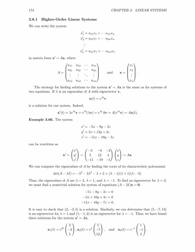
174 CHAPTER 3. LINEAR SYSTEMS
3.8.1 Higher-Order Linear SystemsWe can write the system
x′1 = a11x1 + · · · a1nxnx′2 = a21x1 + · · · a2nxn
...x′n = an1x1 + · · · annxn
in matrix form x′ = Ax, where
A =
a11 a12 · · · a1na21 a22 · · · a2n...
... . . . ...an1 an2 · · · ann
and x =
x1x2...xn
.
The strategy for finding solutions to the system x′ = Ax is the same as for systems oftwo equations. If λ is an eigenvalue of A with eigenvector v,
x(t) = eλtv
is a solution for our system. Indeed,
x′(t) = λeλtv = eλt(λv) = eλtAv = A(eλtv) = Ax(t).
Example 3.66. The system
x′ = −5x− 8y − 2z
y′ = 5x+ 12y + 4z
z′ = −11x− 19y − 5z
can be rewritten as
x′ =
x′y′z′
=
−5 −8 −2
5 12 4
−11 −19 −5
xyz
= Ax.
We can compute the eigenvalues of A by finding the roots of its characteristic polynomial
det(A− λI) = −λ3 − 2λ2 − λ+ 2 = (λ− 1)(λ+ 1)(λ− 2).
Thus, the eigenvalues of A are λ = 2, λ = 1, and λ = −1. To find an eigenvector for λ = 2,we must find a nontrivial solution for system of equations (A− 2I)x = 0,
−7x− 8y − 2z = 0
−5x+ 10y + 4z = 0
−11x− 19y − 7z = 0.
It is easy to check that (2,−3, 5) is a solution. Similarly, we can determine that (5,−7, 13)is an eigenvector for λ = 1 and (1,−1, 2) is an eigenvector for λ = −1. Thus, we have foundthree solutions for the system x′ = Ax,
x1(t) = e2t
2
−3
5
,x2(t) = et
5
−7
13
, and x3(t) = e−t
1
−1
2
.

3.8. LINEAR SYSTEMS IN HIGHER DIMENSIONS 175
The Principle of Superposition also holds for higher-order systems. If x1(t) and x2(t)are solutions for x′ = Ax, then
c1x1(t) + c2x2(t)
is a solution for the system, since
d
dt[c1x1(t) + c2x2(t)] = c1
d
dtx1(t) + c2
d
dtx2(t)
= c1Ax1(t) + c2Ax2(t)
= A[c1x1(t) + c2x2(t)].
Consequently,
x(t) = c1e2t
2
−3
5
+ et
5
−7
13
+ c3e−t
1
−1
2
is a solution for our system. This is, in fact, the general solution for the system.
Although we shall not cover the notions of linear independence, canonical matrices, andchange of coordinates for Rn, the same ideas that we used for systems first-order lineardifferential equations in R2 carry over to Rn.The necessary linear algebra is covered in anygood linear algebra course. Also, see Chapters 5 and 6 in [12].
Example 3.67. Let us see how the linear algebra works in the previous example. If weform the matrix
T =
2 5 1
−3 −7 −1
5 13 2
from the eigenvectors of A, we can convert the system x′ = Ax to the system
y′ = (T−1AT )y 1 −3 −2
−1 1 1
4 1 −1
−5 −8 −2
5 12 4
−11 −19 −5
2 5 1
−3 −7 −1
5 13 2
y,
=
2 0 0
0 1 0
0 0 −1
y,
which we can immediately solve:
y(t) = c1e2t
1
0
0
+ c2et
0
1
0
+ c3e−t
0
0
1
.
Multiplying our solution by T yields the general solution
x(t) = Ty = c1e2t
2
−3
5
+ et
5
−7
13
+ c3e−t
1
−1
2
,
the solution to the system x′Ax.

176 CHAPTER 3. LINEAR SYSTEMS
3.8.2 The Geometry of SolutionsIn Section 3.6, we classified all of the geometry of the solutions for planar systems using thetrace-determinant plane. The geometry for linear systems in three variables is a bit morecomplicated. For a system
x′ = a1x+ a1y + a3z
y′ = b1x+ b2y + b3z
z′ = c1x+ c2y + c3z,
our solutions curves live in R3, and there is simply a lot more room to move around inthree dimensions than in two dimensions. The origin is still an equilibrium solution for asystem of linear differential equations in three variables. The origin is a stable equilibriumsolution if any solution x(t) approaches 0 = (0, 0, 0) as t→ ∞; otherwise, 0 is an unstableequilibrium solution. In the case of planar systems, an unstable solution is a nodal saddle,a nodal source, a spiral source, or a source with a single unstable line. In the case of R3, wecould have a stable line of solutions and an unstable plane of solutions. In this case, allsolutions of the system with initial condition lying on the stable line would approach theorigin as t → ∞, but all solutions with initial conditions that are a nonzero point on theunstable plane would move away from the origin.
Example 3.68. In Example 3.66, we had solutions
x1(t) = e2t
2
−3
5
,x2(t) = et
5
−7
13
, and x3(t) = e−t
1
−1
2
.
The straight line through the origin and the point (1,−1, 2) is a stable line. That is, forany initial condition x(0) = (x0, y0, z0) lying on this line, our solution will tend toward theorigin as t → ∞. On the other hand, the plane spanned by (2,−3, 5) and (5,−7, 13) isunstable plane. Solutions on this plane move away from the origin as t → ∞. Of course,(0, 0, 0) is an equlibrium solution for our system. We say that the origin is a saddle in thisexample (Figure 3.69).
z-axis
T
(1,−1, 2)
Figure 3.69: A saddle in R3
Example 3.70. For the system
x′ =
0 1 0
−1 0 0
0 0 −1
x

3.8. LINEAR SYSTEMS IN HIGHER DIMENSIONS 177
we have a very different type of unstable equilibrium solution. The eigenvalues of this matrixare λ = ±i and λ = −1. Thus, a solution satisfying the initial condition x(0) = (x0, y0, z0)is given by
x(t) = x0
cos t− sin t
0
+ y0
sin tcos t0
+ z0e−t
0
0
1
.
If z0 = 0, then our initial condition is in the xy-plane and all of the solutions lie on circlescentered at the origin. On the other hand, if x0 = 0 and y0 = 0, we have a stable line ofsolutions lying along the z-axis. In fact, each solution that does not lie on the stable linelies on a cylinder in R3 given by x2 + y2 = r2 for some constant r > 0. These solutionsspiral towards the circular solution of radius r in the xy-plane if z0 = 0 (Figure 3.71).
Figure 3.71: A spiral center in R3
Example 3.72. For an example of a stable plane and an unstable line, let us consider thesystem
x′ =
−1 1 0
−1 −1 0
0 0 1
x = Ax.
The characteristic equation of the matrix A is
λ3 + λ2 − 2 = (λ− 1)(λ2 + 2λ+ 2) = 0.
Thus, the eigenvalues of A are λ = 1 and λ = −1± i. Solving
[A− (−1 + i)]x = 0
gives us an eigenvector (1, i, 0) for λ = −1 + i. Since1
i
0
=
1
0
0
+ i
0
1
0
,

178 CHAPTER 3. LINEAR SYSTEMS
we will let v1 = (1, 0, 0) and v2 = (0, 1, 0). Since v3 = (0, 0, 1) is an eigenvector for λ = 1,our system has solution
x(t) = x0e−t
cos t− sin t
0
+ y0e−t
sin tcos t0
+ z0et
0
0
1
,
where x(0) = (x0, y0, z0). If z0 = 0, our initial condition lies in the xy-plane and solutioncurves sprial in towards the origin. Thus, we have a stable plane. On the other hand, ifx0 = 0 and y0 = 0 but z0 = 0, then our solution approaches ±∞ as t → ∞. In this case,the z-axis is an unstable line (Figure 3.73).
Figure 3.73: A spiral saddle in R3
For an example of a stable equilibrium solution at the origin, consider the system
x′ =
λ1 0 0
0 λ2 0
0 0 λ3
x,
where λ3 < λ2 < λ1 < 0. For an initial condition (x0, y0, z0) with at least one coordinatenonzero, the corresponding solution tends towards the origin tangentially to the x-axis ast→ ∞ (Figure 3.74).

3.8. LINEAR SYSTEMS IN HIGHER DIMENSIONS 179
Figure 3.74: A sink in R3
Changing the system that in ExampleExample 3.72 to be
x′ =
−1 1 0
−1 −1 0
0 0 −1
x,
we obtain the solution satisfying the initial condition x(0) = (x0, y0, z0) to be
x(t) = x0e−t
cos t− sin t
0
+ y0e−t
sin tcos t0
+ z0e−t
0
0
1
,
where x(0) = (x0, y0, z0). In this case, all solutions will approach the origin as t→ ∞.
3.8.3 The Double Spring-Mass Systems RevisitedLet us return to our spring-mass system x′ = Ax, where
A =
0 0 1 0
0 0 0 1
−2k/m1 k/m1 0 0
k/m2 −2k/m2 0 0
.
To keep matter simple, we will assume that m1 = m2 = k = 1. Thus, our matrix nowbecomes
A =
0 0 1 0
0 0 0 1
−2 1 0 0
1 −2 0 0
.

180 CHAPTER 3. LINEAR SYSTEMS
The characteristic polynomial of A is
det(A− λI) = λ4 + 4λ2 + 3 = (λ2 + 1)(λ2 + 3).
Thus the eigenvalues of A are λ = ±i and λ = ±i√3. We can find eigenvectors
v1 =
i/√3
−i/√3
−1
1
,v2 =
−i/
√3
i/√3
−1
1
,v3 =
−i−i1
1
,v4 =
i
i
1
1
,
corresponding to the eigenvalues λ1 = i√3, λ2 = −i
√3, λ3 = i, λ4 = −i, respectively.
Consequently, the general solution to our system is
x(t) = c1ei√3tv1 + c1e
−i√3tv2 + c1e
itv3 + c1e−itv4;
however, this form of the solution is not very useful. By examining real and imaginary partsof ei
√3tv1 and c1e
itv3, we can rewrite the solution as
x(t) = c1
cos
√3t
− cos√3t
−√3 sin
√3t√
3 sin√3t
+ c2
− sin
√3t
sin√3t
−√3 cos
√3t√
3 cos√3t
+ c3
cos tcos t− sin t− sin t
+ c4
sin tsin tcos tcos t
.
If we have the following initial conditions,
x1(0) = 0
x2(0) = 0
x′1(0) = x3(0) = 2
x′2(0) = x4(0) = 2,
we can determine c1 = c2 = c3 = 0 and c4 = 2. Thus, the solution to our initial valueproblem is
x(t) =
2 sin t2 sin t2 cos t2 cos t
,
and the two masses will oscillate with a frequency of one and an amplitude of two. We leavethe details as an exercise.
3.8.4 Important Lessons
•
x′1 = a11x1 + · · · a1nxnx′2 = a21x1 + · · · a2nxn
...x′n = an1x1 + · · · annxn

3.8. LINEAR SYSTEMS IN HIGHER DIMENSIONS 181
can be written in matrix form x′ = Ax, where
A =
a11 a12 · · · a1na21 a22 · · · a2n...
... . . . ...an1 an2 · · · ann
and x =
x1x2...xn
.
• As in the case of R2, we can solve the system x′ = Ax by finding eigenvalues andeigenvectors for A.
• The Principle of Superposition holds for higher-order systems. If x1(t) and x2(t) aresolutions for x′ = Ax, then
c1x1(t) + c2x2(t)
is a solution for the system.
• The geometry for system in R3 is more complicated than the planar case. However,the solutions are usually characterized by stable lines or stable planes.
3.8.5 Exercises
1. Solve the system
x′ = −5x+ 15y − 4z
y′ = −x+ 5y − z
z′ = 4x− 6y + 3z
x(0) = −1
y(0) = 2
z(0) = 0
2. Find the general solution of the system
x′1 = 6x1 + 9x2 + x3 + 4x4
x′2 = −x1 + x2 + x3
x′3 = 3x1 + 8x2 + 4x3 + 4x4
x′4 = −3x1 − 8x2 − 7x3 − 5x4
3. Let ax′′ + bx′ + cx = 0, where a = 0 and b2 − 4ac = 0.(a) Show that x1(t) = e−bt/2a is a solution to ax′′ + bx′ + cx = 0.(b) Assume that
y = v(t)x1(t) = v(t)e−bt/2a
is a solution to ax′′ + bx′ + cx = 0 and show that v(t) = c1 + c2t. Thus,
x(t) = c1e−bt/2a + c2te
−bt/2a
is a general solution for ax′′ + bx′ + cx = 0.

182 CHAPTER 3. LINEAR SYSTEMS
4. Consider the equation
y′′ − (2α− 1)y′ + α(α− 1)y = 0.
Determine all values of α, if any, for which all solutions tend toward zero as t → ∞. Also,determine the values of α, if any, for which all nonzero solutions become unbounded ast→ ∞.
5. Solve each of the following initial value problems.(a)
y′′ − 2y′ + 5y = 0
y(π/2) = 0
y′(π/2) = 2
(b)
9y′′ − 12y′ + 4y = 0
y(0) = 2
y′(0) = −1
(c)
y′′ + 8y′ − 9y = 0
y(1) = 1
y′(1) = 0
(d)
y′′ + 2ay′ + (a2 + 1)y = 0
y(0) = 1
y′(0) = 0
6. Reduction of Order. Suppose that x1(t) is a solution (not identically zero) to the equation
x′′ + p(t)x′ + q(t)x = 0.
(a) Assume that x(t) = v(t)x1(t) is a solution to x′′ + p(t)x′ + q(t)x = 0 and derive theequation
x1v′′ + (2x′1 + px1)v
′ = 0. (3.14)
(b) Let u = v′ and show that ((3.16)) is a first-order linear differential equation in u.(c) Show that x1(t) = 1/t is a solution to
2t2x′′ + 3tx′ − x = 0 (3.15)
for t > 0 and find a second linearly independent solution to ((3.17)).
7. Euler Equations. An important class of second-order linear differential equations areequations of the form
t2y′′ + αty′ + βy = 0,
where t > 0 and α and β are real constants. An equation of this form is called an Eulerequation.

3.9. THE MATRIX EXPONENTIAL 183
(a) Show that the substitution x = ln t transforms an Euler equation into an equation ofconstant coefficients. Hint: Show that
dy
dt=dx
dt
dy
dx
d2y
dt2=
(dx
dt
)2 d2y
dx2+d2x
dt2dy
dx.
(b) Solve the equationt2y′′ + 4ty′ + 2y = 0.
3.8.6 Project
3.9 The Matrix ExponentialConsider the linear system
x′ = −17x− 46y − 7z
y′ = 8x+ 21y + 3z
z′ = −7x− 15y − z
The matrix associated with this system is
A =
−17 −46 −7
8 21 3
−7 −15 −1
.
The characteristic polynomial of A is
p(λ) = det(A− λI) = λ3 − 3λ2 + 3λ− 1 = (λ− 1)3
hence, there is only a single eigenvalue λ = 1. Moreover, we can only find a single linearlyindependent eigenvector (1,−1, 4). Thus,
x(t) = ce−t
1
−1
4
is a solution to our system. However, this is not the general solution to the system. Wecan only solve initial value problems where the initial condition lies on the line through theorigin containing the vector (1,−1, 4). To construction a general solution to our system, wewill need two other linearly independent solutions.
3.9.1 The Exponential of a MatrixOur goal is to construct a solution to the initial value problem
x′ = Axx(0) = x0,
where A is an n× n matrix. Recalling that the solution to the initial value problem
x′ = kx

184 CHAPTER 3. LINEAR SYSTEMS
x(0) = x0
is x(t) = x0ekt, we might guess that a solution to the initial value problem
x′ = Axx(0) = x0
has the formx(t) = etAx0
if we can make sense of the expression etA.We will define the exponential of A using the power series for et. Thus,
eA = I +A+1
2!A2 +
1
3!A3 + · · · =
∞∑k=0
1
k!Ak,
where A is an n × n matrix, where A0 = I by convention. Each term makes sense in ourdefinition since each is an expression of n × n matrices; however, there are some issuessurrounding the convergence of the power series. A series, even a series whose individualterms are matrix expressions, converges if and only if its partial sums,
SN =
N∑k=0
1
k!Ak
converge. Although we shall not provide a proof, the matrix exponential eA converges forall A.
Example 3.75. Let us compute the exponential of
A =
(s 0
0 t
).
Actually, this is quite easy,
eA = I +A+1
2!A2 +
1
3!A3 + · · ·
=
(1 0
0 1
)+
(s 0
0 t
)+
1
2!
(s2 0
0 t2
)+
1
3!
(s3 0
0 t3
)+ · · ·
=
(1 + s+ s2/2! + s3/3! + · · · 0
0 1 + t+ t2/2! + t3/3! + · · ·
)=
(es 0
0 et
).
Theorem 3.76. If A is an n× n matrix, then
d
dtetA = AetA.
Proof. We simply need to differentiate
etA = I + tA+t2
2!A2 +
t3
3!A3 + · · ·

3.9. THE MATRIX EXPONENTIAL 185
term by term.3 However,
d
dtetA =
d
dt
(I + tA+
t2
2!A2 +
t3
3!A3 + · · ·
)= A+ tA2 +
t2
2!A3 + · · ·
= A
(I + tA+
t2
2!A2 +
t3
3!+ · · ·
)= AetA.
Corollary 3.77. Let A be an n×n matrix. Then x(t) = etAx0 is the solution to the initialvalue problem
x′ = Axx(0) = x0
Proof. The corollary follows immediately from Theorem 3.76. If x(t) = etAx0, then
x′(t) =d
dt
(etAx0
)=
d
dt
(etA)
x0 = AetAx0 = Ax(t).
Thus, solving linear systems is simply a matter of computing matrix exponentials. Theproblem is that matrix exponentials may not be so easy to compute.
Example 3.78. The matrix
A =
(4 4
−9 −8
)has repeated eigenvalues λ = −2. If we try to compute etA, then
etA = I + tA+t2
2!A2 +
t3
3!A3 + · · ·
=
(1 0
0 1
)+ t
(4 4
−9 −8
)+t2
2!
(4 4
−9 −8
)2
+t3
3!
(4 4
−9 −8
)3
+ · · ·
=
(1 0
0 1
)+ t
(4 4
−9 −8
)+t2
2!
(−20 −16
−36 28
)+t3
3!
(64 48
−108 −80
)+ · · ·
=
(1 + t− 20t2/2! + 64t3/3! + · · · 4t− 16t2/2! + 48t3/3! + · · ·−9t− 36t2/2!− 108t3/3! + · · · 1− 8t+ 28t2/2!− 80t3/3! + · · ·
).
It is not at all clear that this series converges to a matrix whose entries can be expressedin terms of elementary functions.
Now let us see how we can use the matrix exponential to solve a linear system as wellas invent a more direct way to compute the matrix exponential.
Theorem 3.79. Let λ be an eigenvalue of an n×n matrix A. If v is an eigenvector for λ,then etAv = eλtv.
3Since we are differentiating an infinite series, we still need to show that differentiating term by term issomething that can be done. We will, however, leave the details to a course in advanced calculus.

186 CHAPTER 3. LINEAR SYSTEMS
Proof. Since v is an eigenvalue for λ, we know that Av = λv. Using mathematicalinduction, we can show that An has eigenvalue λn with associated eigenvector v. Indeed,
Anv = A(An−1v) = A(λn−1v) = λn−1Av = λnv.
Hence,
etAv =
(I + tA+
t2
2!A2 +
t3
3!A3 + · · ·
)v
= v + tAv +t2
2!A2v +
t3
3!A3v + · · ·
= v + tλv +t2
2!λ2v +
t3
3!λ3v + · · ·
=
(I + tλ+
t2
2!λ2 +
t3
3!λ3 + · · ·
)v
= eλtv.
The matrix exponential shares several properties with the function exponential functionex that we studied in calculus.
Theorem 3.80. Let A and B be n× n matrices. Then
1. AeA = eAA;
2. if AB = BA, then eAeB = eA+B;
3. eA has inverse e−A.
Proof. To prove (1), we can simply expand both sides of the equality in a power series,
AeA = A
(I +A+
1
2!A2 +
1
3!A3 + · · ·
)= A+A2 +
1
2!A3 +
1
3!A4 + · · ·
=
(I +A+
1
2!A2 +
1
3!A3 + · · ·
)A
= eAA.
Proving (2) is a only bit more complicated if we notice that the binomial expansion holdsfor matrices,
(A+B)n =n∑
k=0
(n
k
)AkBn−k,
where (n
k
)=
n!
k!(n− k)!,
providing AB = BA.
eA+B =∞∑n=0
1
n!(A+B)n
=
∞∑n=0
1
n!
(n∑
k=0
(n
k
)AkBn−k
)

3.9. THE MATRIX EXPONENTIAL 187
=
∞∑n=0
(n∑
k=0
1
k!(n− k)!AkBn−k
)
=
( ∞∑n=0
1
n!An
)( ∞∑n=0
1
n!Bn
)= eAeB.
Simply expand each series out to see that this is true. Part (3) follows directly from Part(2), since A and −A commute.
Example 3.81. Now let us compute etA once again for
A =
(4 4
−9 −8
).
First notice thatA = λI + (A− λI).
Since the identity matrix I commutes with every matrix, we know that
etA = et(λI+(A−λI)) = etλIet(A−λI).
We also know that eλtI = eλtI by Example 3.75. Thus,
etA = et(λI+(A−λI)) = etλIet(A−λI) = eλtet(A−λI).
The matrix A has repeated eigenvalue λ = −2. Consequently,
A− λI = A+ 2I =
(6 4
−9 −6
),
and (A− λI)2 is the zero matrix. Thus,
etA = eλtet(A−λI)
= eλt(I + t(A− λI) +
t2
2!(A− λI)2 +
t2
3!(A− λI)3 + · · ·
)= e−2t
(I + t(A+ 2I) +
t2
2!(A+ 2I)2 +
t2
3!(A+ 2I)3 + · · ·
)= e−2t (I + t(A+ 2I))
= e−2t
(1 + 6t 4t
−9t −6t
).
Our example suggests at the following proposition. We leave the proof of this propositionas an exercise.
Proposition 3.82. If A is an n × n matrix with a single eigenvalue λ, then there existsnonnegative integer k < n such that
etA = eλt(I + t(A− λI) +
t2
2!(A− λI)2 + · · ·+ tk
k!(A− λI)k
).

188 CHAPTER 3. LINEAR SYSTEMS
Example 3.83. We are now ready return to our original system x′ = Ax, where
A =
−17 −46 −7
8 21 3
−7 −15 −1
.
This matrix has a single eigenvalue λ = 1. It is easy to show that the only nonzero powersof A− λI = A− I are
(A+ I) =
−18 −46 −7
8 20 3
−7 −15 −2
(A+ I)2 =
5 13 2
−5 −13 −2
20 52 8
.
Therefore,
etA = et(I + t(A+ I) +
t2
2!(A+ I)2
)
= et
1− 18t+ 5t2/2 −46t+ 13t2/2 −7t+ t2
8t− 5t2/2 1 + 20t− 13t2/2 3t− t2
−7t+ 10t2 −15t+ 26t2 1− 2t+ 4t2
.
Now, to compute three linearly independent solutions for x′ = Ax, we simply compute etAvfor three linearly independent vectors. We will use the standard basis vectors
e1 =
1
0
0
, e2 =
0
1
0
, e3 =
0
0
1
.
Thus, the general solution to our system is
x(t) = c1e−t
1− 18t+ 5t2/2
8t− 5t2/2
−7t+ 10t2
+ c2e−t
−46t+ 13t2/2
1 + 20t− 13t2/2
−15t+ 26t2
+ c3e−t
−7t+ t2
3t− t2
1− 2t+ 4t2
.
3.9.2 Generalized EigenvaluesExample 3.84. Consider the system x′ = Ax, where
A =
7 −1 2
18 −2 6
−9 2 −1
.
The characteristic polynomial of A is
det(A− λI) = λ3 − 4λ2 + 5λ− 2 = (λ− 1)2(λ− 2).
The eigenvalue λ1 = 1 has eigenvector v1 = (2, 6,−3) and the eigenvalue λ2 = 2 haseigenvector v2 = (1, 3,−1). Thus, we can find two linearly independent solutions in thiscase
x1(t) = et
2
6
−3
and x2(t) = e2t
1
3
−1
.

3.9. THE MATRIX EXPONENTIAL 189
Since λ1 = 1 has multiplicity two and we can find only one linearly independent eigenvector,it is not possible to apply Proposition 3.82 in this case.
If we consider the exponential
etAv = eλ1tet(A−λ1I)v
= eλ1t
(v + t(A− λ1I)v +
t2
2!(A− λ1I)
2v +t2
3!(A− λ1I)
3v + · · ·)
where v,v1 and v2 are linearly independent, our goal is to choose v for which the seriestruncates. That is, we must look for vectors v such that (A− λ1I)
kv = (A− I)kv = 0. Ifk = 1, then (A−λ1I)v = (A−I)v = 0, which means that v is an eigenvector. Thus, v mustbe a multiple of v1 = (2, 6,−3) in this case. Since we already know that the eigenspaceassociated with this eigenvector has dimension one and is generated by v1, we must considerhigher powers.
Since
(A− λI) = (A− I) =
6 −1 2
18 −3 6
−9 2 −2
,
we have
(A− λI)2 = (A− I)2 =
0 1 2
0 3 6
0 −1 −2
.
The nullspace of this matrix has dimension two. Certainly, v1 = (2, 6,−3) is in the nullspaceof (A − I)2, since it is the nullspace of A − I. We wish to find a vector in the nullspacethat is not a multiple of the vector v1 that is also in the nullspace of A − I. The vectorv = (0, 1, 0) will do. Now our series truncates,
x3(t) = etAv= eλ1tet(A−λ1I)v= eλ1t (v + t(A− λ1I)v)
= eλ1t
0
1
0
+ t(A− I)
0
1
0
= et
t
1 + 3t
−t
We now have a general solution for our system,
x(t) = c1et
2
6
−3
+ c2e2t
1
3
−1
+ c3et
t
1 + 3t
−t
.
If λ is an eigenvalue of A and (A − λI)pv = 0 for some p ≥ 1, then v is called ageneralized eigenvector of A. When eigenvalues have algebraic multiplicity greater thanone, we can compute extra solutions by looking for vectors in the nullspace of (A−λI)p forp > 1. The following theorem tells us that this is always possible. We leave the proof ofthe theorem as an exercise in linear algebra.

190 CHAPTER 3. LINEAR SYSTEMS
Theorem 3.85. Suppose that λ is an eigenvalue of A with multiplicity q. Then there existsan integer p ≤ q such that the dimension of the nullspace of (A− λI)p is q.
We now have a procedure for finding q linearly independent solutions corresponding toan eigenvalue λ of multiplicity q.
1. Find the smallest integer p such that the nullspace of (A− λI)p has dimension q.
2. Find a basis v1, . . . ,vq for the nullspace of (A− λI)p.
3. For each vj (j = 1, 2, . . . , q), we have the solution
xj(t) = etAvj
= eλt(
vj + t(A− λI)vj + · · ·+ tp−1
(p− 1)!(A− λI)p−1vj .
).
This procedure works for complex eigenvalues as well as real. If λ = α+ iβ has eigenvectorz = x + iy, then set x = Re z and y = Im z.
3.9.3 Important Lessons
• If A is an n× n matrix, we define the exponential of A to be
eA = I +A+1
2!A2 +
1
3!A3 + · · · =
∞∑k=0
1
k!Ak.
• If A is an n× n matrix, thend
dtetA = AetA.
• Let A be an n × n matrix. Then x(t) = etAx0 is the solution to the initial valueproblem
x′ = Axx(0) = x0
• Let λ be an eigenvalue of an n × n matrix A. If v is an eigenvector for λ, thenetAv = eλtv.
• Let A and B be n× n matrices. Then
AeA = eAA; if AB = BA, then eAeB = eA+B; eA is nonsingular with inverse e−A.
• If A is an n×n matrix with a single eigenvalue λ, then there exists nonnegative integerk < n such that
etA = eλt(I + t(A− λI) +
t2
2!(A− λI)2 + · · ·+ tk
k!(A− λI)k
).
• Suppose that λ is an eigenvalue of A with multiplicity q. Then there exists an integerp ≤ q such that the dimension of the nullspace of (A− λI)p is q.

3.9. THE MATRIX EXPONENTIAL 191
• The procedure for finding q linearly independent solutions corresponding to an eigen-value λ of multiplicity q is the following.
Find the smallest integer p such that the nullspace of (A−λI)p has dimension q. Find a basis v1, . . . ,vq for the nullspace of (A− λI)p. For each vj (j = 1, 2, . . . , q), we have the solution
xj(t) = etAvj
= eλt(
vj + t(A− λI)vj + · · ·+ tp−1
(p− 1)!(A− λI)p−1vj .
).
The procedure works for complex eigenvalues as well as real. If λ = α + iβ haseigenvector z, then set x = Re z and y = Im z.
3.9.4 Exercises1. Solve the system
x′ = −5x+ 15y − 4z
y′ = −x+ 5y − z
z′ = 4x− 6y + 3z
x(0) = −1
y(0) = 2
z(0) = 0
2. Find the general solution of the system
x′1 = 6x1 + 9x2 + x3 + 4x4
x′2 = −x1 + x2 + x3
x′3 = 3x1 + 8x2 + 4x3 + 4x4
x′4 = −3x1 − 8x2 − 7x3 − 5x4
3. Let ax′′ + bx′ + cx = 0, where a = 0 and b2 − 4ac = 0.(a) Show that x1(t) = e−bt/2a is a solution to ax′′ + bx′ + cx = 0.(b) Assume that
y = v(t)x1(t) = v(t)e−bt/2a
is a solution to ax′′ + bx′ + cx = 0 and show that v(t) = c1 + c2t. Thus,
x(t) = c1e−bt/2a + c2te
−bt/2a
is a general solution for ax′′ + bx′ + cx = 0.
4. Consider the equation
y′′ − (2α− 1)y′ + α(α− 1)y = 0.
Determine all values of α, if any, for which all solutions tend toward zero as t → ∞. Also,determine the values of α, if any, for which all nonzero solutions become unbounded ast→ ∞.

192 CHAPTER 3. LINEAR SYSTEMS
5. Solve each of the following initial value problems.(a)
y′′ − 2y′ + 5y = 0
y(π/2) = 0
y′(π/2) = 2
(b)
9y′′ − 12y′ + 4y = 0
y(0) = 2
y′(0) = −1
(c)
y′′ + 8y′ − 9y = 0
y(1) = 1
y′(1) = 0
(d)
y′′ + 2ay′ + (a2 + 1)y = 0
y(0) = 1
y′(0) = 0
6. Reduction of Order. Suppose that x1(t) is a solution (not identically zero) to the equation
x′′ + p(t)x′ + q(t)x = 0.
(a) Assume that x(t) = v(t)x1(t) is a solution to x′′ + p(t)x′ + q(t)x = 0 and derive theequation
x1v′′ + (2x′1 + px1)v
′ = 0. (3.16)(b) Let u = v′ and show that ((3.16)) is a first-order linear differential equation in u.(c) Show that x1(t) = 1/t is a solution to
2t2x′′ + 3tx′ − x = 0 (3.17)
for t > 0 and find a second linearly independent solution to ((3.17)).
7. Euler Equations. An important class of second-order linear differential equations areequations of the form
t2y′′ + αty′ + βy = 0,
where t > 0 and α and β are real constants. An equation of this form is called an Eulerequation.(a) Show that the substitution x = ln t transforms an Euler equation into an equation of
constant coefficients. Hint: Show thatdy
dt=dx
dt
dy
dx
d2y
dt2=
(dx
dt
)2 d2y
dx2+d2x
dt2dy
dx.
(b) Solve the equationt2y′′ + 4ty′ + 2y = 0.

3.9. THE MATRIX EXPONENTIAL 193
3.9.5 Project

4
Second-Order Linear Equations
4.1 Homogeneous Linear EquationsA differential equation of the form
a(t)x′′ + b(t)x′ + c(t)x = g(t)
is called a second-order linear differential equation. We will first consider the case
ax′′ + bx′ + cx = 0,
where a, b, and c are constants and a = 0. An equation of this form is said to be homoge-neous with constant coefficients. We already know how to solve such equations since wecan rewrite them as a system of first-order linear equations. Thus, we can find the generalsolution of a homogeneous second-order linear differential equation with constant coeffi-cients by computing the eigenvalues and eigenvectors of the matrix of the correspondingsystem.
4.1.1Recall the RC circuits that we studied earlier (see Section 1.3). Such circuits contained avoltage source, a capacitor, and a resistor. A battery or generator is an example of a voltagesource, and a toaster or an electric stove is an example of something that might providea resistance in a circuit. Capacitors store an electrical charge and are used in electronicflashes for cameras. We will now add an inductor such as a solenoid, a coil that generatesa magnetic field. Inductor applications include transformers, power supplies, televisions,radios. Our new circuit is called an RLC circuit (Figure 4.1).
E(t)
+
−
R
L
C
I(t)
Figure 4.1: An RLC Circuit
194

4.1. HOMOGENEOUS LINEAR EQUATIONS 195
Current, I(t), is the rate at which a charge flows through this circuit and is measuredin amperes or amps. We assign a direction to the current, and a current flowing in theopposite direction will be given negative values. The impressed voltage, E(t), is measuredin volts, the resistance R is measured in ohms, and the capacitance C is measured in farads.The charge on the capacitor Q(t) at time t is measured in coulombs. Inductance on thecoil, L, is measured in henrys.
The following laws from physics govern how our circuit behaves.
• I =dQ
dt.
• The voltage drop across a resistor is IR (Ohm’s Law).
• The voltage drop across a capacitor is Q/C.
• The voltage drop across an inductor is L(dI/dt).
• In a closed circuit the impressed voltage is equal to the sum of the voltage drops inthe rest of the circuit (Kirchhoff’s Second Law).
Applying Kirchhoff’s Second Law to our circuit, we have the differential equation
LdI
dt+RI +
1
CQ = E(t) (4.1)
orLQ′′ +RQ′ +
1
CQ = E(t).
Differentiating both sides of (4.1), we have
LI ′′ +RI ′ +1
CI = E′(t).
For example, we might consider an RLC circuit with R = 1, L = 1, and C = 1. At t = 0when both I(0) = 0 and I ′(0) = Q(0) = 0, the impressed voltage on the circuit is given byE(t) = sin(t). Our equation becomes
I ′′ + I ′ + I = E′(t) = cos t.
This is an example of a second-order linear differential equation.
4.1.2 Second-Order Linear EquationsSuppose that we have a homogeneous second-order linear differential equation with constantcoefficients,
ax′′ + bx′ + cx = 0. (4.2)
Since we can rewrite this equation as a system of first-order linear equations,
x′ = y
y′ = − cax− b
ay.
we can find the general solution by computing the eigenvalues and eigenvectors of the matrixof the corresponding system. Solutions of a linear system x′ = Ax often include terms ofthe form ert. It makes sense that solutions to equation (4.2) take the same form.

196 CHAPTER 4. SECOND-ORDER LINEAR EQUATIONS
Example 4.2. Consider the equation
x′′ + 7x′ + 10x = 0. (4.3)
If we assume that a solution is of the form ert, we can substitute this expression into theleft-hand side of (4.3) to obtain
d2
dt2ert +
d
dt7ert + 10ert = r2ert + 7rert + 10ert
= (r2 + 7r + 10)ert
= (r + 5)(r + 2)ert.
Since ert is never zero, we find that (r+5)(r+2) = 0 or r = −5 or −2. Thus, we have twosolutions
x1(t) = e−5t and x2(t) = e−2t.
By the Principle of Superposition,
x(t) = c1x1(t) + c2x2(t) = c1e−5t + c2e
−2t (4.4)
is a solution to x′′ + 7x′ + 10x = 0.Indeed, this is the general solution of our second-order equation since we have a one-to-
one correspondence between the solutions of
x′′ + 7x′ + 10x = 0
and the system
x′ = y
y′ = −10x− 7y.
The matrix associated with this system
A =
(0 1
−10 −7
)has eigenvalues λ1 = −5 and λ2 = −2 with eigenvectors v1 = (1,−5) and v2 = (1,−2),respectively. Consequently, the solution to our system is(
x(t)
y(t)
)= c1e
−5t
(1
−5
)+ c2e
−2t
(1
−2
),
which agrees with (4.4).
In general, suppose thatax′′ + bx′ + cx = 0,
where a = 0. Applying the startegy in Example 4.2, we can find the general solution forthis equation by finding the roots of the quadratic polynomial aλ2 + bλ+ c,
λ = −−b±√b2 − 4ac
2a.
If b2 − 4ac > 0, we have real roots
λ1 =−b+
√b2 − 4ac
2aand λ2 =
−b−√b2 − 4ac
2a,

4.1. HOMOGENEOUS LINEAR EQUATIONS 197
and the solution to our second-order differential equation is
x(t) = c1eλ1t + c2e
λ2t, (4.5)
where c1 and c2 are arbitrary constants.To prove that equation (4.5) is indeed the general solution to the second-order equation
ax′′+ bx′+ cx = 0, we can study the equivalent system of linear equations. If we let y = x′,the corresponding linear system is x′ = Ax, where
A =
(0 1
−c/a −b/a
).
The characteristic polynomial of A is
p(λ) = det(A− λI) = λ2 +b
aλ+
c
a.
The roots of p(λ) are the same as the roots of aλ2 + bλ + c. If b2 − 4ac > 0, we have realroots
λ1 =−b+
√b2 − 4ac
2aand λ2 =
−b−√b2 − 4ac
2a.
We can find eigenvectors
v1 =
(1
(−b+√b2 − 4ac )/2a
)=
(1
λ1
)v1 =
(1
(−b−√b2 − 4ac )/2a
)=
(1
λ2
)for λ1 and λ2, respectively. Thus, the general solution to the system of differential equationsx′ = Ax is
x(t) =(x(t)
y(t)
)=
(x(t)
x′(t)
)= c1e
λ1t
(1
λ1
)+ c2e
λ2t
(1
λ2
),
which agrees with (4.5).
Example 4.3. Now let us solve the initial value problem
x′′ + 4x′ + 5x = 0
x(0) = 1
x′(0) = 1.
Again, we will assume that our solution has the form x(t) = ert. Substituting this functioninto our differential equation, we find that
0 = x′′ + 4x′ + 5x = r2ert + 4rert + 5ert = (r2 + 4r + 5)ert.
As with the real case, r2 + 4r + 5 = 0 or
r =−4±
√−4
2= −2± i.
Thus, we can find a solution
x(t) = e(−2+i)t = e−2teit = e−2t(cos t+ i sin t).

198 CHAPTER 4. SECOND-ORDER LINEAR EQUATIONS
The real and imaginary parts of our solution are
x1(t) = e−2t cos tx2(t) = e−2t sin t,
respectively. We claim that both x1(t) and x2(t) are solutions to our differential equation.Indeed, since x(t) = x1(t) + ix2(t) is a solution,
0 = ax′′ + bx′ + cx
= a(x1 + ix2)′′ + b(x1 + ix2)
′ + c(x1 + ix2)
= (ax′′1 + bx′1 + cx1) + i(ax′′2 + bx′2 + cx2).
Since the real part and the imaginary part of x(t) must both be zero, we can conclude thatax′′1+bx
′1+cx1 = 0 and ax′′2+bx′2+cx2 = 0. Therefore, the general solution to our equation
isx(t) = c1e
−2t cos t+ c2e−2t sin t.
To apply our initial conditions x(0) = 1 and x′(0) = 1, we first calculate
x′(t) = −2e−2t(c1 cos t+ sin t) + e−2t(−c1 sin t+ c2 cos t).
Thus,
1 = x(0) = c1
1 = x′(0) = −2c1 + c2,
and c1 = 1 and c2 = 3. Hence, the solution to our initial value problem is
x(t) = e−2t cos t+ 3e−2t sin t.
As before, the corresponding linear sytem is x′ = Ax, where
A =
(0 1
−c/a −b/a
).
If b2 − 4ac < 0, the eigenvalue of A are λ = α+ iβ and λ = α− iβ, where
α = − b
2aand β =
√4ac− b2
2a.
The vector v = (1, α + iβ) is an eigenvector for λ. Thus, a solution to our system ofdifferential equations is
x(t) =(x(t)
y(t)
)=
(x(t)
x′(t)
)= e(α+iβ)t
(1
α+ iβ
)= eαt(cosβt+ i sinβt)
(1
α+ iβ
)= eαt
(cosβt
α cosβt− β sinβt
)+ ieαt
(sinβt
α sinβt+ β cosβt
).

4.1. HOMOGENEOUS LINEAR EQUATIONS 199
Taking the real and imaginary parts of x(t), we obtain two real solutions to the system,x1(t) = eαt cosβt and x2(t) = eαt sinβt. Therefore, the general solution to ax′′1+bx′1+cx1 =0 is
x(t) = c1eαt cosβt+ c2e
αt sinβt.
4.1.3 Reduction of OrderGiven a second-order linear differential equation with constant coefficients, ax′′+bx′+cx =0, our strategy has been to solve the characteristic equation aλ2 + bλ+ c = 0 to obtaintwo linearly independent solutions. We have covered the case where this equation has twodistinct real solutions as well as when there are complex soluitons, but what if there is onlya single real solution λ = −b/2a.
Example 4.4. Consider the equation
x′′ + 2x′ + x = 0.
If we choose eλt as our guess, we find
x′′ + 2x′ + x = λ2eλt + 2λeλt + eλt
= eλt(λ+ 1)2
= 0.
Thus, λ = −1 and we have a solution x1(t) = e−t. In order to find a general solution tox′′ + 2x′ + x = 0, we must find a second solution that is not a multiple of x1(t) = e−t.
In order to find a general solution to x′′ + 2x′ + x = 0, we must find a second solutionthat is not a multiple of x1(t) = e−t. Since we already know that cx1(t) is a solution toour differential equation, we will try to generalize this observation by replacing c with anonconstant function v(t) and then try to determine v(t) so that v(t)x1(t) is a solution tox′′ + 2x′ + x = 0. Indeed, if
x(t) = v(t)x1(t) = v(t)e−t,
thenx′(t) = v(t)x′1(t) + v′(t)x1(t) = −v(t)e−t + v′(t)e−t
and
x′′(t) = v′′(t)x1(t) + 2v′(t)x′1(t) + v(t)x′′1(t)
= v′′(t)e−t − 2v′(t)e−t + v(t)e−t.
Consequently,
x′′ + 2x′ + x = [v′′e−t − 2v′e−t + ve−t] + 2[−ve−t + v′e−t] + [ve−t]
= e−tv′′
= 0,
and v′′ = 0. Therefore, v = c1t + c2. Letting c1 = 1 and c2 = 0, we can assume thatv(t) = t, and the second solution to our equation is x = te−t. Hence, the general solutionto x′′ + 2x′ + x = 0 is
x(t) = c1e−t + c2te
−t.
We leave it as an exercise to show that our solution agrees with the solution that we wouldobtain from solving the equivalent first-order linear system.

200 CHAPTER 4. SECOND-ORDER LINEAR EQUATIONS
The technique that we have used in Example 4.4 is called reduction of order. We leaveit as an exercise to show that this technique works in general. That is, given a second-orderlinear differential equation
ax′′ + bx′ + cx = 0
such that b2 − 4ac = 0, then the general solution is given by
x(t) = c1eλt + c2te
λt,
where λ = −b/2a.We did a great deal of work finding unique solutions to first-order linear systems of
equations,
x′ = ax+ by
y′ = cx+ dy.
Our efforts are now rewarded. Since each second-order homogeneous system with constantcoefficients can be rewritten as a first-order linear system, we are guaranteed the existenceand uniqueness of solutions.
4.1.4 Important Lessons
• A second-order linear differential equation with constant coefficients is an equation ofthe form
ax′′ + bx′ + cx = 0.
We can guess the solution to this equation. Since we can rewrite this equation asa system of first-order linear differential equations, we can determine the generalsolution to ax′′ + bx′ + cx = 0.
• Suppose thatax′′ + bx′ + cx = 0,
where a = 0 and b2 − 4ac > 0. If the roots of ar2 + br + c are r1 and r2, the generalsolution to this differential equation is
x(t) = c1er1t + c2e
r2t.
• If b2 − 4ac < 0, the differential equation
ax′′ + bx′ + cx = 0
has a general solutionx(t) = c1e
αt cosβt+ c2eαt sinβt,
where α± iβ are the roots of ar2 + br + c = 0.
• If b2 − 4ac = 0, the differential equation
ax′′ + bx′ + cx = 0
has a general solutionx(t) = c1e
−bt/2a + c2te−bt/2a.

4.1. HOMOGENEOUS LINEAR EQUATIONS 201
4.1.5 Exercises1. Find the general solution of each of the following differential equations.
(a) d2y
dx2− y = 0
(b) x′′ − 2x′ + x = 0
(c) y′′ + 5y = 0
(d) d2x
dt2+ 2
dx
dt+ 3x = 0
(e) x′′ − 10x′ + 25x = 0
(f) d2y
dx2− dy
dx+ 2y = 0
(g) y′′ + 8y′ + 16y = 0
(h) d2x
dx2− 2
dx
dt+ 4x = 0
(i) d2Q
dt2− 4
dQ
dt+ 9Q = 0
(j) d2y
dt2+ 6
dy
dt+ 9y = 0
Hint. (a) (c) (e) (g) (i)2. Let ax′′ + bx′ + cx = 0, where a = 0 and b2 − 4ac = 0.(a) Show that x1(t) = e−bt/2a is a solution to ax′′ + bx′ + cx = 0.(b) Assume that
y = v(t)x1(t) = v(t)e−bt/2a
is a solution to ax′′ + bx′ + cx = 0 and show that v(t) = c1 + c2t. Thus,
x(t) = c1e−bt/2a + c2te
−bt/2a
is a general solution for ax′′ + bx′ + cx = 0.
Hint.(a) Observe that
ax′′1 + b′1 + cx1 = a
(−b2a
)2
e−bt/2a + b
(−b2a
)e−bt/2a + ce−bt/2a
= e−bt/2a
(b2
4a− b2
2a+ c
)= e−bt/2a
(−b2 + 4ac
4a
)= 0.
(b) If y = v(t)x1(t) = v(t)e−bt/2a is a solution to our differential equation, then
ay′′ + by′ + cy = a(v′′x1 + 2v′x′1 + vx′′1) + b(v′x1 + vx′1) + cvx1
= av′′x1 + 2av′x′1 + bv′x1 + v(ax′′1 + bx′1 + cx1)
= av′′e−bt/2a +
[2a
(−b2a
)e−bt/2a + be−bt/2a
]v′

202 CHAPTER 4. SECOND-ORDER LINEAR EQUATIONS
= av′′e−bt/2a
= 0.
Since a = 0, we know that v′′ = 0. Hence, v(t) = c1 + c2t.3. Reduction of Order. Suppose that x1(t) is a solution (not identically zero) to the equation
x′′ + p(t)x′ + q(t)x = 0.
(a) Assume that x(t) = v(t)x1(t) is a solution to x′′ + p(t)x′ + q(t)x = 0 and derive theequation
x1v′′ + (2x′1 + px1)v
′ = 0. (4.6)
(b) Let u = v′ and show that (4.6) is a first-order linear differential equation in u.(c) Show that x1(t) = 1/t is a solution to
2t2x′′ + 3tx′ − x = 0 (4.7)
for t > 0 and find a second linearly independent solution to (4.7).
Hint.(a)
x′′ + px′ + qx = (v′′x1 + 2v′x′1 + vx′′1) + p(v′x1 + vx′1) + q(vx1)
= x1v′′ + 2v′x′1 + px1v
′ + v(x′′1 + px′1 + qx1)
= x1v′′ + (2x′1 + px1)v
′
= 0.
(b) If u = v′, then x1u′ + (2x′1 + px1)u = 0.
(c) If x1(t) = 1/t, then
2t2x′′1 + 3tx′1 − x1 = 2t2(2
t3
)+ 3t
(−1
t2
)− 1
t= 0.
If we assume that x = v/t is a second solution, then
2t2x′′ + 3tx′ − x = 2tv′′ − v′ = 0.
If we let u = v′, then a solution of 2tu′ − u = 0 is u =√t and v =
∫ √t dt = 2t3/2/3.
Therefore, the second solution to our equation is
x =v
t=
2
3
√t.
4.1.6 Project
4.2 ForcingHarmonic oscillators such as a spring-mass system (Subsection 1.1.3) or an RLC circuit(Section 4.1) can be modeled with second-order linear differential equations. Indeed, wecan model a spring-mass system with the equation
mx′′(t) + bx′(t) + kx(t) = g(t),

4.2. FORCING 203
where m is the mass, b is the damping coefficient, k is the spring constant, and F (t) = g(t)represents some external force applied to our system. RLC circuits can also be modeledwith provide another example of forcing. If I(t) is the rate at which a charge flows througha circuit (measured in amperes or amps), R is the resistance (measured in ohms), C is thecapacitance (measured in farads), and the inductance, L, is (measured in henrys), then thederivative of the impressed voltage (measured in volts), E(t), is the forcing term
LI ′′ +RI ′ +1
CI = E′(t).
What is different about these two equations are the terms on the righthand side, g(t) andE′(t). Such a term is called a forcing term.
4.2.1 Nonhomogeneous EquationsA nonhomogeneous second-order linear differential equation is an equation of theform
x′′ + p(t)x′ + q(t)x = g(t).
We have already seen how examples of such equations arise when examining models ofharmonic oscillators with forcing terms. Our goal is to be able to solve such equations. Ingeneral, these equations can be difficult to solve for an arbitrary function g(t). Before weattempt to find solutions for some of the more common functions that might occur for g(t),let us derive some fundamental facts about second-order linear differential equations.
Theorem 4.5. Suppose that
x′′ + p(t)x′ + q(t)x = g(t) (4.8)
has solutions x1 = x1(t) and x2 = x2(t). Then x1(t)−x2(t) is a solution of the homogeneouslinear differential equation
x′′ + p(t)x′ + q(t)x = 0.
Proof. Since x1 and x2 are solutions of (4.8), we know that
x′′1 + p(t)x′1 + q(t)x1 = g(t)
x′′2 + p(t)x′2 + q(t)x2 = g(t).
Thus,
d2
dt2(x1 − x2) + p(t)
d
dt(x1 − x2) + q(t)(x1 − x2)
=
(d2x1dt2
+ p(t)dx1dt
+ q(t)x1
)−(d2x2dt2
+ p(t)dx2dt
+ q(t)x2
)= g(t)− g(t) = 0.
We can use Theorem Theorem 4.5 to derive the fact that the general solution to
x′′ + p(t)x′ + q(t)x = g(t). (4.9)
can be written in the formx = xh + xp,
where yh is the general solution of the homogeneous equation
x′′ + p(t)x′ + q(t)x = 0,
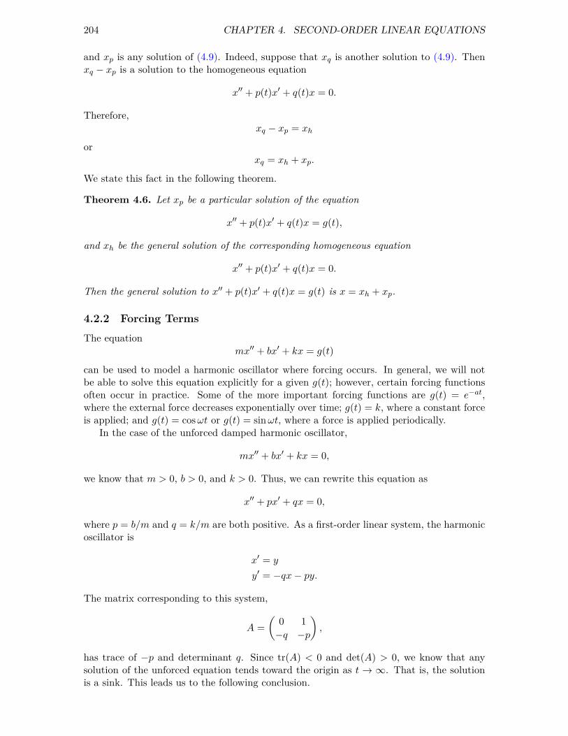
204 CHAPTER 4. SECOND-ORDER LINEAR EQUATIONS
and xp is any solution of (4.9). Indeed, suppose that xq is another solution to (4.9). Thenxq − xp is a solution to the homogeneous equation
x′′ + p(t)x′ + q(t)x = 0.
Therefore,xq − xp = xh
orxq = xh + xp.
We state this fact in the following theorem.
Theorem 4.6. Let xp be a particular solution of the equation
x′′ + p(t)x′ + q(t)x = g(t),
and xh be the general solution of the corresponding homogeneous equation
x′′ + p(t)x′ + q(t)x = 0.
Then the general solution to x′′ + p(t)x′ + q(t)x = g(t) is x = xh + xp.
4.2.2 Forcing TermsThe equation
mx′′ + bx′ + kx = g(t)
can be used to model a harmonic oscillator where forcing occurs. In general, we will notbe able to solve this equation explicitly for a given g(t); however, certain forcing functionsoften occur in practice. Some of the more important forcing functions are g(t) = e−at,where the external force decreases exponentially over time; g(t) = k, where a constant forceis applied; and g(t) = cosωt or g(t) = sinωt, where a force is applied periodically.
In the case of the unforced damped harmonic oscillator,
mx′′ + bx′ + kx = 0,
we know that m > 0, b > 0, and k > 0. Thus, we can rewrite this equation as
x′′ + px′ + qx = 0,
where p = b/m and q = k/m are both positive. As a first-order linear system, the harmonicoscillator is
x′ = y
y′ = −qx− py.
The matrix corresponding to this system,
A =
(0 1
−q −p
),
has trace of −p and determinant q. Since tr(A) < 0 and det(A) > 0, we know that anysolution of the unforced equation tends toward the origin as t → ∞. That is, the solutionis a sink. This leads us to the following conclusion.

4.2. FORCING 205
Theorem 4.7. Supposex′′ + px′ + qx = g(t)
has solution x = xh + xp, where p > 0 and q > 0. If
x = xh + xp
is the general solution to the equation, then
x = xh + xp → xp
as t→ ∞.
In other words, all solutions of a damped harmonic oscillator with nonzero damping areessentially the same for large values of t.
4.2.3 The Method of Undetermined CoefficientsExample 4.8. Let us solve the differential equation
x′′ + 5x′ + 4x = 1, (4.10)
a harmonic oscillator with a constant forcing function. It is easy to check that the generalsolution to the homogeneous equation
x′′ + 5x′ + 4x = 0
isxh = c1e
−t + c2e−4t.
A particular solution to (4.10) is given by xp = 1/4. Thus, the general solution is
x(t) = c1e−t + c2e
−4t +1
4.
As t→ ∞, all solutions approach the constant solution x = 1/4 (Figure 4.9).
2 4 6 8 10t
-1
1
2
x(t)dx/dt
Figure 4.9: Solutions to x′′ + 5x′ + 4x = 1

206 CHAPTER 4. SECOND-ORDER LINEAR EQUATIONS
Example 4.10. Now let us consider a more complicated example. Suppose that we wishto solve
x′′ + 5x′ + 4x = e−2t. (4.11)This is the equation of a harmonic oscillator with a forcing function that decreases expo-nentially with time. We already know the solution to the homogeneous equation. We willuse the method of undetermined coefficients to find a particular solution to (4.11). Itis reasonable to guess that a particular solution will have the form
xp = Ae−2t.
Substituting this expression into (4.11), we find that
e−2t = x′′p + 5x′p + 4xp = 4Ae−2t − 10Ae−2t + 4Ae−2t = −2Ae−2t.
Hence, A = −1/2. Therefore, the solution that we seek is
x = c1e−t + c2e
−4t − 1
2e−2t.
Again, all solutions approach zero as t→ ∞ (Figure 4.11).
2 4 6 8 10t
-1
1
2
x(t)dx/dt
Figure 4.11: Solutions to x′′ + 5x′ + 4x = e−2t
Example 4.12. Now let us examine what happens if we have a periodic forcing function.Let us assume that the particular solution to the equation
x′′ + 5x′ + 4x = 2 cos t.
takes the formxp = A cos t+B sin t.
Then
x′p = −A sin t+B cos tx′′p = −A cos t−B sin t.
Substituting these expressions into the differential equation, we see that
2 cos t = x′′p + 5x′p + 4xp

4.2. FORCING 207
= (−A cos t−B sin t) + 5(−A sin t+B cos t) + 4(A cos t+B sin t)= (3A+ 5B) cos t+ (−5A+ 3B) sin t.
We must solve the following system of equations to find a particular solution:
3A+ 5B = 2
−5A+ 3B = 0.
The solution of this system is A = 3/17 and B = 5/17. Consequently,
xp =3
17cos t+ 5
17sin t
is a particular solution to x′′ + 5x′ + 4x = 2 cos t. The general solution to our equation is
x = c1e−t + c2e
−4t +3
17cos t+ 5
17sin t.
The solutions to this equation are given in Figure 4.13.
2 4 6 8 10t
-1
1
2
x(t)dx/dt
Figure 4.13: Solutions to x′′ + 5x′ + 4x = 2 cos t
Example 4.14. As a final example, consider the
x′′ + 5x′ + 4x = e−t.
Recall that the solution to the homogeneous equation x′′ + 5x′ + 4x = 0 is
xh = c1e−t + c2e
−4t.
Our guess of xp(t) = Ae−t for a particular solution will no longer work since e−t is a solutionto the homogeneous equation. We must therefore consider a function of a different form.Such a function must yield a multiple of e−t when differentiated. The simplest such functionis of the form
xp = Ate−t.
Using this guess,
e−t =d2
dt2Ate−t + 5
d
dtAte−t + 4Ate−t

208 CHAPTER 4. SECOND-ORDER LINEAR EQUATIONS
= A(−e−t − e−t + te−t) + 5A(e−t − te−t) + 4Ate−t
= 3Ae−t.
Thus, A = 1/3 and our general solution is
x = c1e−t + c2e
−4t +1
3te−t.
Solutions to the differential equation x′′ + 5x′ + 4x = e−t are given in Figure 4.15.
2 4 6 8 10t
-1
1
2
x(t)dx/dt
Figure 4.15: Solutions to x′′ + 5x′ + 4x = e−t
4.2.4 A StrategyWe outline a general strategy for choosing xp for the Method of Undetermined Coefficientsin Table 4.16. Here s = 0, 1, 2 is the smallest integer that will ensure that no term in xp isa solution of the corresponding homogeneous equation.
g(t) xpPn(t) = ant
n + · · ·+ a1t+ a0 ts(Antn + · · ·+A1t+A0)
Pn(t)eαt ts(Ant
n + · · ·+A1t+A0)eαt
Pn(t)eαt
sinβtcosβt tseαt[(Ant
n + · · ·+A1t+A0) cosβt
+(Bntn + · · ·+B1t+B0) sinβt]
Table 4.16: Particular solutions of x′′ + px′ + qx = g(t).
4.2.5 Important Lessons
• A nonhomogeneous second-order linear differential equation is an equationof the form
x′′ + p(t)x′ + q(t)x = g(t).
Forced harmonic oscillators and RLC circuits provide good examples of nonhomoge-neous second-order linear differential equations.

4.2. FORCING 209
• Suppose thatx′′ + p(t)x′ + q(t)x = g(t)
has solutions x1 = x1(t) and x2 = x2(t). Then x1(t) − x2(t) is a solution of thehomogeneous linear differential equation
x′′ + p(t)x′ + q(t)x = 0.
• Let xp be a particular solution of the equation
x′′ + p(t)x′ + q(t)x = g(t),
and xh be the general solution of the corresponding homogeneous equation
x′′ + p(t)x′ + q(t)x = 0.
Then the general solution to x′′ + p(t)x′ + q(t)x = g(t) is x = xh + xp. In particular,if the solution to x′′ + p(t)x′ + q(t)x = 0 has a sink at the origin, all solutions of theequation x′′ + p(t)x′ + q(t)x = g(t) approach xp(t) as t→ ∞.
• The Method of Undetermined Coefficients is useful for solving the equation x′′ +p(t)x′ + q(t)x = g(t), when g is of the form
g(t) = Pn(t)eαt
sinβtcosβt
4.2.6 Exercises
1. Find the solution of the initial-value problem
y′′ + 6y′ + 8y = cos 3ty(0) = 0
y′(0) = 0.
Hint. The solution to the homogeneous equation y′′ + 7y′ + 10y = 0 is
yh = c1e−4t + c2e
−2t.
Using the method of undetermined coefficients, we can find a particular solution
yp =2
235(18 sin 3t− cos 3t).
Thus, the general solution is
y = yh + yp = c1e−4t + c2e
−2t +2
235(18 sin 3t− cos 3t).
Applying the initial conditions y(0) = 0 and y′(0) = 0, we have
y = − 16
235e−4t +
18
235e−2t +
2
235(18 sin 3t− cos 3t).

210 CHAPTER 4. SECOND-ORDER LINEAR EQUATIONS
2. Compute the solution of the initial value problem
y′′ + 4y = 3 cos 2ty(0) = y′(0) = 0.
Hint. The solution to the homogeneous equation, y′′ + 4y = 0 is
yh = c1 cos 2t+ c2 sin 2t.
The complex version of the equation is
y′′ + 4y = 3e2it.
Assume that the particular solution to this equation is yc = ate2it. We include a factorof t, since e2it is a solution to the homogeneous equation. Substituting yc and y′′c into thedifferential equation, we have
y′′c + 4yc = 4a(i− t)e2it + 4ate2it = 4aie2it = 3e2it.
Thus, a = 3/(4i) = −3i/4. Taking the real part of
yc = −3
4it(cos 2t+ i sin 2t),
we haveyp =
3
4t sin 2t.
Therefore the general solution is
y = yh + yp = c1 cos 2t+ c2 sin 2t+3
4t sin 2t.
Applying the initial conditions y(0) = y′(0) = 0, we find that c1 = c2 = 0 and
y =3
4t sin 2t.
3. Use the complex method to find a particular solution to
y′′ + 7y′ + 10y = −4 sin 3t.
Write your solution as a function of cosine. What is the amplitude, the period, and thefrequency of your solution?Hint. If we assume that the complex solution has form yc = Ae3it, then
y′′c + 7y′c + 10yc = A(1 + 21i)e3it = −4e3it,
andA =
−4
1 + 21i=
−2 + 42i
221.
In polar form,A = |A|eiϕ =
4√442
eiϕ,
where ϕ = π + arctan(−21). Thus, yc = Ae3it = 4ei(3t+ϕ)/√442. Using the imaginary part
of this solution, we obtain
y =4√442
sin 3t+ ϕ =4√442
cos(3t− θ),
where θ = ϕ−π/2 = π/2+arctan(−21). The amplitude is 4/√442, the period is 2π/3, and
the frequency is 3/2π.

4.2. FORCING 211
4. We define two functions, f(t) and g(t), to be linearly independent on an open intervalI = (a, b) if there do not exist nonzero constants c1 and c2 such that
c1f(t) + c2g(t) = 0
for all t ∈ I. Otherwise, f(t) and f(t) are linearly dependent. Suppose that f(t) and g(t)are solutions to the homogeneous linear equation
y′′ + py′ + qy = 0.
Show that f(t) and g(t) are linearly dependent on an interval I = (a, b) if and only ifW [f, g](t) ≡ 0.
Hint. Suppose that that f(t) and g(t) are linearly dependent on an interval I = (a, b).Then one function is a multiple of the other, say f(t) = cg(t). Thus, f ′(t) = cg′(t).
W (f, g)(t) = det(f(t) g(t)
f ′(t) g′(t)
)= f(t)g′(t)− f ′(t)g(t) = cg(t)g′(t)− cg′(t)g(t) = 0.
Conversely, suppose that
W (f, g)(t) = det(f(t) g(t)
f ′(t) g′(t)
)= 0,
for all t in (a, b). If g = 0, then 0f = g and the two functions are linearly dependent. Assumethat g(t0) = 0 for some t0 in (a, b). Since g is differentiable, it must also be continuous andthere is some interval (c, d) contained in (a, b) such that t0 ∈ (c, d) and g does not vanishon this interval. Therefore,
d
dt
(f
g
)=f ′g − fg′
g2= −W (f, g)
g2= 0,
and f/g is constant on the interval (c, d). Thus, f(t0) = cg(t0) and f(t′0) = cg′(t0). Since fand cg are both solutions to the differential equation y′′ + py′ + qy = 0 and have the sameinitial condition, f(t) = cg(t) for all t ∈ (a, b) by the existence and uniqueness theorem.Consequently, f and g are linearly dependent.5. Abel’s Theorem. If y1 and y2 are solutions of the homogeneous equation
y′′ + p(t)y′ + q(t)y = 0,
where p and q are continuous on an open interval I = (a, b), show that
W [y1, y2](t) = c exp(−∫p(t) dt
),
for some constant c that depends on y1 and y2 but not on t.(a) Use Abel’s Theorem to find the Wronskian of 2t2y′′ + 3ty′ − y = 0 up to a constant
multiple, where t > 0.(b) Prove Abel’s Theorem.
Hint.

212 CHAPTER 4. SECOND-ORDER LINEAR EQUATIONS
(a) We can rewrite 2t2y′′ + 3ty′ − y = 0 as
y′′ +3
2ty′ − 1
2t2y = 0.
Since p(t) = 1/2t, Abel’s Theorem tells us that
W [y1, y2](t) = c exp(−∫
3
2tdt
)= c exp
(−3
2ln t)
= ct−3/2.
(b) Since y1 and y2 are solutions to our differential equation, we know that
y′′1 + p(t)y′1 + q(t)y1 = 0
y′′2 + p(t)y′2 + q(t)y2 = 0.
Multiplying the first equation by y2 and the second equation by y1 and subtracting,we obtain
(y1y′′2 − y′′1y2) + p(t)(y1y
′2 − y′1y2) = 0. (4.12)
IfW (t) =W (y1, y2)(t) = y1y
′2 − y′1y2,
thenW ′ = y1y
′′2 − y′′1y2,
and equation (4.12) becomesW ′′ + p(t)W = 0.
This equation is separable with solution
W (t) = c exp(−∫p(t) dt
),
6. The Method of Variation of Parameters. In this problem we will describe another methodof finding a particular solution to a nonhomogeneous equation,
y′′ + p(t)y′ + q(t)y = f(t), (4.13)
if we know know that the general solution to the homogeneous equation y′′+p(t)y′+q(t)y = 0is
yh = c1y1 + c2y2.
(a) Assume that a particular solution of (4.13) has the form
yp(t) = u1(t)y1(t) + u2(t)y2(t),
whereu′1(t)y1(t) + u′2(t)y2(t) = 0.
Substitute yp into the left-hand side of (4.13) to show that
u′1(t)y′1(t) + u′2(t)y
′2(t) = f(t).
(b) Show that
u′1(t) =−y2(t)f(t)W [y1, y2](t)
u′2(t) =y1(t)f(t)
W [y1, y2](t),
where W [y1, y2](t) = y1(t)y′2(t)− y2(t)y
′1(t) is the Wronskian of y1 and y2.

4.2. FORCING 213
(c) If p, q, and f are continuous on an interval I, show that
u1(t) = −∫ t
t0
y2(s)f(s)
W [y1, y2](s)ds
u2(t) =
∫ t
t0
y1(s)f(s)
W [y1, y2](s)ds
for any point t0 in I. Consequently, a particular solution to (4.13) is
yp = −y1(t)∫ t
t0
y2(s)f(s)
W [y1, y2](s)ds+ y2(t)
∫ t
t0
y1(s)f(s)
W [y1, y2](s)ds.
(d) Find the general solution of the differential equation
y′′ + 4y = 3 csc t.
Hint.(a) If yp = u1y1 + u2y2, then
y′p = u′1y1 + u1y′1 + u′2y2 + u2y
′2 = u1y
′1 + u2y
′2
y′′p = u′1y′1 + u1y
′′1 + u′2y
′2 + u2y
′′2 .
Substituting these expressions into equation (4.13), we have
y′′p + py′p + qyp = (u′1y′1 + u1y
′′1 + u′2y
′2 + u2y
′′2) + p(u1y
′1 + u2y
′2)
+ q(u1y1 + u2y2)
= u1[y′′1 + py′1 + qy1] + u2[y
′′2 + py′2 + qy2] + u′1y
′1 + u′2y
′2
= u′1y′1 + u′2y
′2
= f(t).
(b) If we solve the system
u′1(t)y1(t) + u′2(t)y2(t) = 0
u′1(t)y′1(t) + u′2(t)y
′2(t) = f(t).
for u′1 and u′2, we obtain
u′1(t) =−y2(t)f(t)W [y1, y2](t)
u′2(t) =y1(t)f(t)
W [y1, y2](t).
(c) Integrate the two equations from part (2).(d) The general solution to the homogeneous equation y′′ + 4y = 0 is
yh = c1 cos 2t+ c2 sin 2t.
To find a particular solution, assume that the solution has the form
yp = u1(t) cos 2t+ u2(t) sin 2t.

214 CHAPTER 4. SECOND-ORDER LINEAR EQUATIONS
By part (2)
u′1(t) = −3 cos t
u′2(t) =3
2csc t− 3 sin t.
Integrating, we obtain
u1(t) = −3 sin t
u2(t) =3
2ln | csc t− cot t|+ 3 cos t.
Therefore,
yp(t) = u1(t)y1(t) + u2(t)y2(t)
= −3 sin t cos 2t+[3
2ln | csc t− cot t|+ 3 cos t
]sin 2t,
and the general solution is
y = yh + yp
= c1 cos 2t+ c2 sin 2t− 3 sin t cos 2t+[3
2ln | csc t− cot t|+ 3 cos t
]sin 2t.
4.2.7 Project
4.3 Sinusoidal Forcing
If we consider different forcing functions g(t) for the equation
x′′ + px′ + qx = g(t),
functions that are periodic are especially important. Recall that a function g(t) is periodicif
g(t+ T ) = g(t)
for all t and some fixed constant T . The most familiar periodic functions are
g(t) = sinωt and g(t) = cosωt.
The period for each of these two functions is 2π/ω and the frequency is ω/2π. These twofunctions share the additional property that their average value is zero. That is,
1
T
∫ T
0g(t) dt = 0.
We say that sinusoidal forcing occurs in the differential equation
x′′ + px′ + qx = A cosωt+B sinωt.

4.3. SINUSOIDAL FORCING 215
4.3.1 ComplexificationGiven a second-order linear differential equation
ax′′ + bx′ + cx = A cosωt+B sinωt,
we can use Euler’s formula, eiβt = cosβt+ i sinβt to derive a particular solution. That is,we will assume that our particular solution has the form
xc = xRe + ixIm
and use the properties of complex numbers.1
Example 4.17. Let us consider the equation
x′′ + 6x′ + 5x = sin 2t. (4.14)
The solution to the corresponding homogeneous equation, x′′ + 6x′ + 5x = 0, is
xh = c1e−5t + c2e
−t.
To find a particular solution, we can use the method of undetermined coefficients and assumethat the solution has the form
xp = A cos 2t+B sin 2t.
If we carry out the appropriate calculations, we will obtain a particular solution
xp = − 12
145cos 2t+ 1
145sin 2t.
Thus, the general solution is
x = xh + xp = c1e−5t + c2e
−t − 12
145cos 2t+ 1
145sin 2t.
Notice that all solutions of (4.14) will approach the particular solution as t→ ∞.
Example 4.18. Now let us solve (4.14) using complex numbers. If we assume that theequation has a complex solution of the form xc = xRe + ixIm, then
d2
dt2xc + 6
d
dtxc + 5xc =
d2
dt2(xRe + ixIm) + 6
d
dt(xRe + ixIm) + 5(xRe + ixIm)
= e2it
= cos 2t+ i sin 2t.
Equating the real and imaginary parts of this equation, we obtain
x′′Re + 6x′Re + 5xRe = cos 2tx′′Im + 6x′Im + 5xIm = sin 2t.
Thus, if we can find a complex solution, we can find a solution to
x′′ + 6x′ + 5x = sin 2t
1If complex numbers make you uncomfortable, the alternative is to become an expert in trigonometricidentities

216 CHAPTER 4. SECOND-ORDER LINEAR EQUATIONS
simply by examining the imaginary part of the solution.Now let us assume that our solution has the form xc = Ae2it. Then
x′′c + 6x′c + 5xc = −4Ae2it + 12Aie2it + 5Ae2it
= (1 + 12i)Ae2it
= (1 + 12i)A(cos 2t+ i sin 2t).
Equating the real and imaginary parts of this equation, we obtain
x′′Re + 6x′Re + 5xRe = cos 2tx′′Im + 6x′Im + 5xIm = sin 2t
and we immediately see that
A =1
1 + 12i=
1
145− 12
145i.
Therefore, the complex solution to
x′′ + 6x′ + 5x = e2it
is
xc = Ae2it
=
(1
145− 12
145i
)· (cos 2t+ i sin 2t)
=
(1
145cos 2t+ 12
145sin 2t
)+ i
(− 12
145cos 2t+ 1
145sin 2t
).
The imaginary part of this function is
xIm = − 12
145cos 2t+ 1
145sin 2t,
which is the particular solution that we have been seeking. Thus, our general solution agreeswith what we found in Example 4.17.
4.3.2 Qualitative AnalysisWe can use the complex solution of ax′′ + bx′ + cx = A cosωt + B sinωt to analyze thequalitative behavior of solutions.
Example 4.19. We discovered that the complex solution of
x′′ + 6x′ + 5x = e2it
to be xc = Ae2it, where A = (1− 12i)/145. Let us rewrite A in polar form. Since
|A| = 1√145
,
we know thatA =
1√145
eiθ,

4.3. SINUSOIDAL FORCING 217
where θ = arctan(−12) ≈ −1.4877. Therefore,
xc = Ae2it =1√145
eiθe2it =1√145
ei(2t+θ).
Our particular solution is the imaginary part of xc,
xp(t) =1√145
sin(2t+ θ) =1√145
cos(2t+ θ − π
2
)=
1√145
cos (2t− ϕ) ,
where ϕ ≈ 3.058451. We say that ϕ is the phase angle of our solution. The amplitude ofour solution is 1/
√145 and the period is π (Figure 4.20).
π 2π 3π 4π 5πt
−0. 05
0. 05
x(t)
Figure 4.20: Steady state solution to x′′ + 6x′ + 5x = sin 2t
The corresponding first order system for the differential equation
x′′ + px′ + qx = g(t),
is
x′ = y
y′ = −qx− py + g(t).
This is a nonautonomous system, and the tangent vector of a solution curve in the phaseplane depends not only on the position (x, y), but also on the time t. In other words, thedirection field changes with time. Since the direction field changes with time, two solutionswith the same (x, y) value at different times can follow different paths. Consequently, solu-tions can cross each other in the xy-plane without violating the Existence and UniquenessTheorem.
Example 4.21. Consider the harmonic oscillator that is modeled by the differential equa-tion
x′′ + 2x′ + 17x = −2 sin 3t. (4.15)
The solution to the homogeneous equation x′′ + 2x′ + 17x = 0 is
xh = c1e−t cos 4t+ c2e
−t sin 4t

218 CHAPTER 4. SECOND-ORDER LINEAR EQUATIONS
The complex version of this equation is
x′′ + 2x′ + 17x = −2e3it,
and we will use the Method of Undetermined Coefficients and assume that we can find aparticular solution of the form xc = Ae3it. Substituting xc into equation (4.15), we findthat
(8 + 6i)Ae3it = −2e3it.
Thus, xc is a solution if
A =−2
8 + 6i= − 4
25+
3
25i
We have
xc(t) =
(− 4
25+
3
25i
)(cos 3t+ i sin 3t)
=
(− 4
25cos 3t− 3
25sin 3t
)+ i
(3
25cos 3t− 4
25sin 3t
).
The imaginary part of this function is the solution that we seek,
xp =3
25cos 3t− 4
25sin 3t.
Thus, the general solution to (4.15) is
x(t) = c1e−t cos 4t+ c2e
−t sin 4t+3
25cos 3t− 4
25sin 3t.
Now suppose that x(0) = 0 and x′(0) = 0. We can quickly determine that
x′(t) = c1e−t(4 cos 4t− sin 4t) + c2e
−t(− cos 4t− 4 sin 4t)− 12
25cos 3t− 9
25sin 3t
To solve this initial value problem, we must solve the linear system
c1 +3
25= 0
−4c1 − c2 −9
25= 0.
We obtain c1 = −3/25 and c2 = 3/25, and the solution to our initial value problem is
x(t) = − 3
40e−2t cos 4t+ 3
80e−2t sin 4t+
3
40cos 2t− 3
20sin 2t.
The graph of our solution is given in Figure 4.22.

4.3. SINUSOIDAL FORCING 219
π 2π 3πt
−0. 2
−0. 1
0. 1
0. 2
x(t)
Figure 4.22: Solution to x′′ + 2x′ + 17x = −2 sin 3t, x(0) = 0, x′(0) = 0
Since y = x′(t), we can now graph the solution curve in the phase plane (Figure 4.23).Notice how the solution curve can intersect itself. The restoring force and damping areproportional to x and y = x′, respectively. When x and y are close to the origin, theexternal force is as large or larger than the restoring and damping forces. In this part ofthe xy-plane, the external force overcomes the damping and pushes the solution away fromthe origin.
-0.2 -0.1 0.1 0.2x
-0.6
-0.4
-0.2
0.2
0.4
0.6
y
Figure 4.23: Phase Plane for x′′ + 2x′ + 17x = −2 sin 3t, x(0) = 0, x′(0) = 0
On the other hand, suppose we have initial conditions x(0) = 2 and x′(0) = 2, we cansolve the linear system
c1 +3
25= 2
−4c1 − c2 −9
25= 2.

220 CHAPTER 4. SECOND-ORDER LINEAR EQUATIONS
to obtain c1 = 47/25 and c2 = 109/100. Thus, solution to our initial value problem is
x(t) =47
25e−t cos 4t+ 109
100e−t sin 4t+
3
40cos 2t− 3
20sin 2t.
The graph of our solution is given in Figure 4.24.
π 2π 3πt
−1. 0
−0. 5
0. 5
1. 0
1. 5
2. 0
x(t)
Figure 4.24: Solution to x′′ + 2x′ + 17x = −2 sin 3t, x(0) = 2, x′(0) = 2
If we examine the phase plane for this solution (Figure 4.25), we see that the initialdamping and restoring forces are much larger than the external force. Thus, if we are farfrom the origin, the solutions in the xy-plane tend to spiral towards the origin and aresimilar to the solutions of the unforced equation.
-1 -0.5 0.5 1 1.5 2x
-6
-4
-2
2
y
Figure 4.25: Phase Plane for x′′ + 2x′ + 17x = −2 sin 3t, x(0) = 2, x′(0) = 2
4.3.3 Important Lessons

4.4. FORCING AND RESONANCE 221
• The functions sinωt and g(t) = cosωt are periodic with period 2π/ω and frequencyω/2π. These average value of each of these functions is zero.
• We can use Euler’s formula and complexification to solve the equation
x′′ + px′ + qx = g(t),
where the forcing function g(t) is sinωt or cosωt. Furthermore, we can use complexnumbers to express or solution in the form
x(t) = A cos(ωt− ϕ),
where A is the amplitude of the solution, ω/2π is the frequency of the solution, andϕ is the phase angle.
• If we write the equationx′′ + px′ + qx = g(t),
as a first-order system,
x′ = y
y′ = −qx− py + g(t),
we obtain a nonautonomous system. In this case the direction field changes with time,and two solutions with the same (x, y) value at different times can follow differentpaths. Therefore, solutions can cross each other without violating the Existence andUniqueness Theorem.
• If we are far from the origin, the solutions in the xy-plane tend to spiral towardsthe origin and are similar to the solutions of the unforced equation. When x andy are close to the origin, the external force is as large or larger than the restoringand damping forces. In this part of the xy-plane, the external force overcomes thedamping and pushes the solution away from the origin.
4.3.4 Exercises1. Compute the solution of the initial value problem
y′′ + 4y = 3 cos 2ty(0) = y′(0) = 0.
4.3.5 Project
4.4 Forcing and ResonanceResonance happens when the natural frequency and the forcing frequency of an undampedharmonic oscillator are the same. There are many real world examples of resonance. Forexample, it is possible for an trained singer shatter a champaign glass by simply singingthe correct note (see https://www.youtube.com/watch?v=IZD8ffPwXRo). Shattering a glass bysinging the correct note is can be modeled by an equation of an undamped harmonic os-cillator with sinusoidal forcing. While a certain amount of damping occurs in all physicalsystems, the damping is often so small that it makes sense to use an undamped harmonicoscillator.

222 CHAPTER 4. SECOND-ORDER LINEAR EQUATIONS
4.4.1 ResonanceResonance was responsible for the collapse of the Broughton suspension bridge near Manch-ester, England in 1831. The collapse occurred when a column of soldiers marched in cadenceover the bridge, setting up a periodic force of rather large amplitude. The frequency of theforce was approximately equal to the natural frequency of the bridge. Thus, the bridgecollapsed when large oscillations occurred. For this reason soldiers are ordered to breakcadence whenever they cross a bridge.
The Millennium Bridge, the first new bridge to span the Thames River in London inover 100 years, is a modern example of how resonance can effect a bridge (Figure 4.26).This pedestrian bridge, which opened to the public in June 2000, was quickly closed afterthe bridge experienced high amplitude horizontal oscillations during periods of high traffic.Studies by designers found that the bridge experienced high amplitude horizontal oscillationsin response to horizontal forcing at a rate of one cycle per second. Typically, people walkat a rate of two steps per second, so the time between two successive steps of the leftfoot is about one second. Thus, if people were to walk in cadence, they would couldset up strong horizontal forcing that would place a destructive load on the bridge. Theengineers did not envision this to be a problem since tourists do not generally march intime. However, a video of tourists crossing the bridge revealed the opposite. When thebridge began oscillating, people tended to walk in cadence in order to keep their balance(https://www.youtube.com/watch?v=gQK21572oSU).
Figure 4.26: The Millennium Bridge
Consider the case of an undamped harmonic oscillator with a sinusoidal forcing function.

4.4. FORCING AND RESONANCE 223
We know that we can model this situation with the second-order linear differential equation
x′′ + ω20x = A cosωt
Since the homogeneous solution to this equation is
xh(t) = c1 cosω0t+ c2 sinω0t,
we can see that the natural frequency of the harmonic oscillator is ω0. This is thefrequency of the oscillations if there is no forcing term. Depending on whether or not thefrequency of the forcing term ω is equal to the natural frequency, we will have two verydifferent situations. If the two frequencies are equal, then they will re-enforce one anotherand we will have resonance. If the two frequencies are close but not equal, we will see thephenomenon of beats. We wish to investigate what happens when the driving frequencyω is equal to the natural frequency and when it is not.
Let us examine the case where the forcing frequency and the natural frequency of theoscillator are the same,
x′′ + ω20x = A cosω0t. (4.16)
Since A cosω0t is a solution to the homogeneous equation x′′ + ω20x = 0, we cannot assume
that a particular solution to equation (4.16) has the form a cosω0t+ b sinω0t. Equivalently,if we use the complex method, we cannot assume that our solution has the form aeiω0t.Therefore, we will look for a complex solution of the form
xc = ateiω0t
for the complex equation that corresponds to (4.16),
x′′ + ω20x = Aeiω0t. (4.17)
In this case,
x′c = a(1 + iω0t)eiω0t
x′′c = a(2iω0 − ω20t)e
iω0t.
Substituting xc and x′′c into the left-hand side of (4.17), we have
x′′c + ω20xc = a(2iω0 − ω2
0t)eiω0t + ω2
0ateiω0t
= 2aiω0eiωt.
In order for xc = ateiω0t to be a solution to (4.17), we must have
a =A
2iω0.
Thus, our solution to the complex form of the differential equation is
xc =A
2iω0teiω0t
= − Ai
2ω0teiω0t
= − Ai
2ω0t(cosω0t+ i sinω0t)
=A
2ω0t sinω0t− i
A
2ω0t cosω0t.
224 CHAPTER 4. SECOND-ORDER LINEAR EQUATIONS
The real part of xc,xp(t) =
A
2ω0t sinω0t,
is a particular solution to (4.16). Thus, our general solution is
x(t) = xh(t) + xp(t) = c1 cosω0t+ c2 sinω0t+A
2ω0t sinω0t.
Example 4.27. Now let us consider the initial-value problem
x′′ + 144x = 4 cos 12tx(0) = 0
x′(0) = 0.
where A = 4 and ω0 = 12. The solution to the homogeneous equation x′′ + 144x = 0 is
xh(t) = c1 cos 12t+ c2 sin 12t.
To find a particular solution to x′′ + 144x = 4 cos 12t, we will use the complex method andtry to find a particular solution to x′′ + 144x = 4e12it. We must assume that the solutionhas the form xc(t) = ate12it, since ae12it is a solution to the homogeneous equation. Asbefore, we have x′′c = a(24i − 144t)e12it. If we substitute xc and x′′c into the left-hand sideof our differential equation, we have
x′′c + 144xc = a(24i− 144t)e12it + 144ate12it = 24aie12it.
Therefore,a =
4
24i= −1
6i,
and our complex solution is
−1
6ie12it = −1
6i(cos 12t+ i sin 12t) =
1
6sin 12t− 1
6i cos 12t.
Taking the real part of our complex solution, we have a particular solution
xp(t) =1
6t sin 12t.
Thus, the general solution to x′′ + 144x = 4 cos 12t is
x(t) = xh(t) + xp(t) = c1 cos 12t+ c2 sin 12t+1
6t sin 12t.
Applying the initial conditions, both c1 = 0 and c2 = 0. Consequently, the solution to theinitial-value problem is
x(t) =1
6t sin 12t.
The graph of this solution is given in Figure 4.28. Notice that our solution grows withtime. This growth is due to the fact that the frequency of the forcing term is equal to thenatural frequency of the oscillator. Since the force pulls and pushes at a frequency equalto the natural frequency of the oscillator, the amplitude increases with time. This type ofbehavior is called resonance.

4.4. FORCING AND RESONANCE 225
π 2π 3π 4πt
−2. 0
−1. 0
1. 0
2. 0
x(t)
Figure 4.28: The solution to x′′ + 4x = 4 sin 2t, x(0) = 0, x′(0) = 0.
4.4.2 Beats or the Case ω = ω0
If the forcing frequency and natural frequency are not equal but close, then we have thephenomenon of beats. For example, a piano tuner uses this phenomenon to make certainthat a particular string is correctly tuned. The tuner will strike a tuning fork which vi-brates at the correct frequency. Next, the tuner hits the poorly tuned piano string. Thismodulation gives rise to beats in the tone that are readily audible. When the string isproperly tuned, the beats will go away. To see another example of beats, watch the videohttps://www.youtube.com/watch?v=pRpN9uLiouI.
To understand the situation where the forcing and natural frequencies differ by a smallamount, ω = ω0, we will first consider the equation,
x′′ + ω20 = A cosωt. (4.18)
The solution to the homogeneous equation x′′ + ω20x = 0 is
xh(t) = c1 cosω0t+ c2 sinω0t.
Since the forcing frequency is not equal to the natural frequency, we can look for a particularsolution to the complex of the form of equation (4.18),
x′′ + ω20 = Aeiωt. (4.19)
If we assume out solution has the form xc = aeiωt and substitute xc into the left-hand sideof (4.19), we find
x′′c + ω20xc = −aω2eiωt + ω2
0aeiωt
= a(ω20 − ω2)eiωt.
Therefore, for xc = aeiωt to be a solution for
x′′ + ω20x = Aeiωt,
we must havea =
A
ω20 − ω2
.

226 CHAPTER 4. SECOND-ORDER LINEAR EQUATIONS
The real part of xc is a particular solution to (4.18),
xp(t) =A
ω20 − ω2
cosωt.
Thus, the general solution to (4.18) is
x(t) = xh(t) + xp(t) = c1 cosω0t+ c2 sinω0t+A
ω20 − ω2
cosωt.
Now let us examine the case where the motion starts at equilibrium. That is, we willinvestigate what happens when x(0) = 0 and x′(0) = 0. In this case, we can easily determinethat c1 = −A/(ω2
0 − ω2) and c2 = 0. Hence the solution to our initial value problem is
x(t) =A
ω20 − ω2
(cosωt− cosω0t). (4.20)
Thus, we have a superposition to two oscillations of different frequencies.To understand how the superposition of the two frequencies works, we will let
ω =ω0 + ω
2
be the mean frequency andδ =
ω0 − ω
2
be the half difference. Since
ω = ω − δ,
ω0 = ω + δ.
we know that
x(t) =A
ω20 − ω2
(cosωt− cosω0t)
=A
(ω + δ)2 − (ω − δ)2(cos[(ω − δ)t]− cos[(ω + δ)t])
=A
4ωδ[cos(ωt− δt)− cos(ωt+ δt)]
=A
4ωδ[cos(ωt) cos(δt) + sin(ωt) sin(δt)− cos(ωt) cos(δt) + sin(ωt) sin(δt)]
=A
4ωδ[2 sin(ωt) sin(δt)]
=A sin δt2ωδ
sinωt.
Thus, we have a sine function, sinωt whose amplitude varies according to |(A/2ωδ) sin δt|,and
x(t) =A sin δt2ωδ
sinωt. (4.21)
Example 4.29. In the initial-value problem
x′′ + 144x = 4 cos(13t) (4.22)x(0) = 0 (4.23)x′(0) = 0, (4.24)

4.4. FORCING AND RESONANCE 227
we have A = 4, ω0 = 12, and ω = 13. The solution to this equation is
x(t) =4
25(cos 12t− cos 13t).
The graph of this solution is given in Figure 4.30 and illustrate the phenomenon of beats.The two frequencies are almost equal and interfere with each other.
π 2π 3π 4π 5π 6π 7π 8π 9π 10πt
−0. 3
−0. 2
−0. 1
0. 1
0. 2
0. 3
x(t)
Figure 4.30: Solution to the initial-value problem (4.22)
In our example, δ = −1/2 and ω = 25/2. The factor sin δt = sin(−t/2) in (4.21)oscillates very slowly in comparison to sin(ω) = sin(25t/2). Thus, we can view the solution(4.21) as a fast oscillation with a frequency ω and amplitude∣∣∣∣A sin δt
2ωδ
∣∣∣∣ = ∣∣∣∣ 825 sin(t
2
)∣∣∣∣ , (4.25)
which oscillates much more slowly. If we superimpose the graph of (4.25) onto the graph inFigure 4.30, we obtain an envelope of the faster oscillation.
π 2π 3π 4π 5π 6π 7π 8π 9π 10πt
−0. 3
−0. 2
−0. 1
0. 1
0. 2
0. 3
x(t)
x(t)|(A/2ωδ)sinδt|
Figure 4.31: Envelope for the initial-value problem (4.22)
4.4.3 Forced Damped Harmonic MotionSince perpetual motion does not really exist, we should consider what happens when weadd some damping to our harmonic oscillator,
x′′ + 2cx′ + ω20x = A cosωt. (4.26)

228 CHAPTER 4. SECOND-ORDER LINEAR EQUATIONS
Example 4.32. Let us consider the differential equation
x′′ + 2x′ + 2x = 3 cos 4t. (4.27)
The corresponding homogeneous equation is
x′′ + 2x′ + 2x = 0,
which has solutionxh(t) = c1e
−t cos t+ c2e−t sin t.
To find a particular solution for the equation (4.27), we will look for a solution of the formxc = ae4it to the equation
x′′ + 2x′ + 2x = 3e4it (4.28)
and then set xp(t) to the real part of the solution. Substituting xc into the lefthand side of(4.28), we obtain
x′′c + 2x′c + 2xc = (−14 + 8i)ae4it = P (4i)ae4it = 3e4it,
where P (λ) = λ2 + 2λ+ 2 is the characteristic polynomial of x′′ + 2x′ + 2x = 0. Therefore,
a =3
P (4i)=
3
−14 + 8i= − 3
130(7 + 4i),
and the solution to the complex equation is
xc = − 3
130(7 + 4i)e4it
= − 3
130(7 + 4i)(cos 4t+ i sin 4t)
=3
130[(−7 cos 4t+ 4 sin 4t) + i(−4 cos 4t− 7 sin 4t)].
Thus, we can determine a particular solution by taking the real part of xc,
xp(t) =3
130(−7 cos 4t+ 4 sin 4t).
The general solution for (4.27) is
x(t) = xh(t) + xp(t) = c1e−t cos t+ c2e
−t sin t+ 3
130(−7 cos 4t+ 4 sin 4t).
It is easy to see that all solutions approach xp(t) as t → ∞ no matter what the initialconditions may be. However, it would be much more useful if we would write the particularsolution in the form
xp(t) = K cos(4t− ϕ)
for some constants K and ϕ rather than a linear combination of cos 4t and sin 4t.
Returning to the general case, the associated homogeneous equation for (4.26) is
x′′ + 2cx′ + ω20x = 0. (4.29)
The characteristic polynomial of (4.29),
P (λ) = λ2 + 2cλ+ ω20, (4.30)

4.4. FORCING AND RESONANCE 229
has rootsλ = −c±
√c2 − ω2
0.
If our harmonic oscillator is undedamped (c < ω0), then the solution to the homogeneousequation (4.29) is
xh = e−ct(c1 cosβt+ c2 sinβt),
where β =√ω20 − c2.
As in Example 4.32, we will look for a particular solution to (4.26) by examining theequivalent complex differential equation. That is, we shall look for a solution of the formxc = aeiωt to the equation
x′′c + 2cx′c + ω20xc = Aeiωt, (4.31)
and then set xp equal to the real part of our solution. Substituting xc into the right-handside of (4.31), we obtain
x′′c + 2cx′c + ω20xc = [(iω)2 + 2c(iω) + ω2
0]aeiωt = P (iω)aeiωt,
where P is the characteristic polynomial (4.30). Thus, equation (4.31) becomes
P (iω)aeiωt = Aeiωt,
andxc(t) = aeiωt =
A
P (iω)eiωt = H(iω)Aeiωt,
whereH(iω) =
1
P (iω).
We say that H(λ) = 1/P (λ) is the transfer function.Let us examine the transfer function more closely to see if we can use it to write our
particular solution in a more useable form. First, let us write
P (iω) = (iω)2 + 2c(iω) + ω20 = (ω2
0 − ω2) + 2icω.
in polar form,P (iω) = Reiϕ = R(cosϕ+ i sinϕ),
whereR =
√(ω2
0 − ω2)2 + 4c2ω2
and ϕ is the angle defined by the equations
cosϕ =ω20 − ω2√
(ω20 − ω2)2 − 4c2ω2
,
sinϕ =2cω√
(ω20 − ω2)2 − 4c2ω2
.
Since 2cω > 0, we know that sinϕ > 0. Equivalently, 0 < ϕ < π. Thus,
ϕ = ϕ(ω) = cot−1
(ω20 − ω2
2cω
).
Therefore, we can write the transfer function as
H(iω) =1
P (iω)=
1
Re−iϕ.

230 CHAPTER 4. SECOND-ORDER LINEAR EQUATIONS
We define the gain to be
G(ω) =1
R=
1√(ω2
0 − ω2)2 + 4c2ω2,
and we will rewrite the transfer function as
H(iω) = G(ω)e−iϕ(ω).
Thus, the solution tox′′c + 2cx′c + ω2
0xc = Aeiωt
isxc(t) = H(iω)Aeiωt = G(ω)Aei(ωt−ϕ). (4.32)
Taking the real part of (4.32), our particular solution is
xp(t) = Re(xc(t)) = G(ω)A cos(ωt− ϕ).
It is now clear that particular solution has the same frequency as the forcing term. Inaddition, xp is out of phase with the driving force by the amount
ϕ = ϕ(ω) = cot−1
(ω20 − ω2
2cω
).
The general solution tox′′ + 2cx′ + ω2
0x = A cosωt
isx(t) = xh(t) + xp(t) = e−ct(c1 cos(ηt) + c2 sin(ηt)) +G(ω)A cos(ωt− ϕ).
Since xh has the factor e−ct, the homogeneous part of the solution quickly decays to zero ast→ ∞. For this reason, xh is called the transient term while xp is called the steady-stateterm.
Example 4.33. Let us examine the steady-state solution of the harmonic oscillator inExample 4.32. We have already determined that the second-order linear differential equation
x′′ + 2x′ + 2x = 3 cos 4t
has solution
x(t) = xh(t) + xp(t) = c1e−t cos t+ c2e
−t sin t+ 3
130(−7 cos 4t+ 4 sin 4t).
The natural frequency is ω0 =√2 ≈ 1.4142 If we choose the initial conditions so that c1 = 0
and c2 = 1, our transient term is
xh(t) = e−ct sinβt = e−t sin t.
Since c = 1, ω = 4, and A = 3, the gain is G(4) ≈ 0.0620, the amplitude of the steadystate solution is G(4) · 4 ≈ 0.2481. The phase is ϕ = ϕ(4) ≈ 2.6224. The solution and thesteady-state solution are given in Figure 4.34. As we can see, transient solutions can bequite large when compared to steady-state solutions.

4.4. FORCING AND RESONANCE 231
π 2π 3πt
−0. 2
−0. 1
0. 1
0. 2
0. 3
0. 4
0. 5
x(t)
xh + xpxp
Figure 4.34: A forced damped harmonic oscillator and the steady-state solution.
Large transient currents can be destructive in electrical circuits. For example, a lightbulb usually burns out when a large transient flows through an already weakened bulb. This,usually occurs at the time the light bulb is turned out or turned off. Large transient currentsare particularly harmful to the hard drive in a computer. For this reason, computers shouldbe left on except in the case that they are not being used for a period of several days.
4.4.4 Important Lessons
• A forced damped harmonic oscillator,
x′′ + 2cx′ + ω20x = A cosωt
has homogeneous solution
xh = e−ct(c1 cos ηt+ c2 sin ηt),
where η =√ω20 − c2. A particular solution is given by
xp(t) = Re(xc(t)) = G(ω)A cos(ωt− ϕ),
where the phase angle ϕ is
ϕ = ϕ(ω) = cot−1
(ω20 − ω2
2cω
)and the gain G is given by
G(ω) =1√
(ω20 − ω2)2 + 4c2ω2
.
• The amplitude and phase of the steady-state solution,
xp(t) = G(ω)A cos(ωt− ϕ),
are determined byω20G =
1√(1− s2)2 +D2s2
,
where ω = sω0 and D = 2c/ω0.

232 CHAPTER 4. SECOND-ORDER LINEAR EQUATIONS
• In an undamped harmonic oscillators with a sinusoidal forcing term, the natural fre-quency of the solution interacts with the frequency of the forcing term. As the fre-quency of the forcing term approaches the natural frequency of the equation, we canobserve a phenomenon called resonance. We can use the equation
x′′ + ω20x = A cosωt
to model an undamped harmonic oscillator with sinusoidal forcing.
• If the driving frequency is not equal to the natural frequency (ω = ω0), we have aparticular solution
xp(t) =A
ω20 − ω2
(cosωt− cosω0t).
If the two frequencies are close, we can see a phenomenon called beats.
• If the driving frequency is equal to the natural frequency, we have a particular solution
xp(t) =A
2ω0t sinω0t
In this case, we can see the resonance phenomenon.
• A forced damped harmonic oscillator,
x′′ + 2cx′ + ω20x = A cosωt
has homogeneous solution
xh = e−ct(c1 cos ηt+ c2 sin ηt),
where η =√ω20 − c2. A particular solution is given by
xp(t) = Re(xc(t)) = G(ω)A cos(ωt− ϕ),
where the phase angle ϕ is
ϕ = ϕ(ω) = cot−1
(ω20 − ω2
2cω
)and the gain G is given by
G(ω) =1√
(ω20 − ω2)2 + 4c2ω2
.
4.4.5 Exercises1. Given the equation
y′′ + 10y = sin 3t,
determine the following.(a) The frequency of the beats.(b) The frequency of the rapid oscillations.(c) Use parts (1) and (2) to sketch a graph of a typical solution.
2.

4.4. FORCING AND RESONANCE 233
(a) Suppose that an opera singer can break a glass by singing a particular note. Will thesinger have to sing a higher note or a lower note to break an identical glass that is halffull of water?
(b) Suppose that both notes are within the opera singer’s range. Will it be harder or easierto break the glass when it is half full of water?
(c) Commercials for a maker of recording tape show a crystal glass being broken by thesound of a recording of an opera singer’s voice. Is this a good test of the quality of thetape? Why or why not?
3. For large t, every solution of
y′′ + py′ + qy = cosωt
oscillates with angular frequency ω and amplitude A given by
A(ω, p, q) =1√
(q − ω2)2 + p2ω2.
That is, the amplitude of A is a function of the parameters ω, p, and q.
(a) Compute ∂A
∂ω.
(b) For fixed p and q, let M(p, q) denote the maximum value of A(ω, p, q) as a function ofω. Compute an expression for M(p, q).
(c) Set q = 1 and plot M(p, q) as a function of p.
(d) Explain why M(p, q) is proportional to 1/p as p→ 0.
4. Let us examine the amplitude and phase of the steady-state solution,
xp(t) = G(ω)A cos(ωt− ϕ),
whereG(ω) =
1√(ω2
0 − ω2)2 + 4c2ω2.
Now let s = ω/ω0 and D = 2c/ω0. These new constants, s and D, measure the ratio of thedriving frequency to the natural frequency and the effect of the damping force, respectively.Thus,
G =1
ω20
√(1− s2)2 +D2s2
orω20G =
1√(1− s2)2 +D2s2
.
This expression shows us how the gain varies as s = ω/ω0 varies. The natural frequency isfixed in
x′′ + 2cx′ + ω20x = A cosωt
and D = 2c/ω0 is proportional to the damping constant.

234 CHAPTER 4. SECOND-ORDER LINEAR EQUATIONS
4.4.6 Project—The Tacoma Narrows Bridge
The History of the Tacoma Narrows Bridge
On July 1, 1940, the Tacoma Narrows Bridge was completed and opened to traffic (Fig-ure 4.35). From the first day of operation, the bridge experienced vertical oscillations ofseveral feet. The bridge received the nickname “Galloping Gertie” for its wild behavior.On the morning of November 7, the bridge began undulating up and down with motions aslarge as three feet. Later, the bridge began to experience torsional oscillations as large as 23degrees. The bridge finally came crashing down at 11:10 a.m. For a long time, the collapseof the Tacoma Narrows Bridge was attributed to resonance. However, we shall soon see thethe story is more complicated.
Figure 4.35: The Tacoma Narrows Bridge
Construction on first Tacoma Narrows Bridge, A.K.A. “Galloping Gertie”, was com-pleted on July 1, 1940, the bridge was opened to traffic (Figure 4.36). Even on the first dayof operation, people driving bridge experienced vertical oscillations of several feet. On themorning of November 7, these vertical oscillations were as large as three feet. Later thatmorning, the bridge began to experience torsional oscillations as great as 23 degrees. Thebridge failed castrophically at 11:10 a.m. with the center span falling into Puget Soundbelow.

4.4. FORCING AND RESONANCE 235
Figure 4.36: The Tacoma Narrows Bridge (2017)
There are many interesting stories connected with the first Tacoma Narrows bridge.One of the insurance policies had been written by a local travel agent who pocketed thepremium and failed to report the $800,000 policy to his company. During sentencing athis trial, he pointed out that bridge officials had planned to cancel all policies in one moreweek after which his crime would have never been discovered. After the collapse of theTacoma Narrows bridge, the governor of the State of Washington announced, “We aregoing to build the exact same bridge, exactly as before.” Theodore Von Kármán, director ofthe Guggenheim Aeronautical Laboratory at the California Institute of Technology and amember of the board of inquiry into the collapse,2 sent a telegram to the governor stating,“If you build the exact same bridge exactly as before, it will fall into the exact same riverexactly as before.”
The Design of the Narrows Bridge
The Tacoma Narrows bridge is a suspension bridge like the Golden Gate bridge. The roadbed of the suspension bridge was hung from vertical cables attached to other cables strungbetween the two towers. If we think of the cables as long springs, it is tempting to modelthe oscillations of the road bed with an harmonic oscillator, and one’s first guess as to thereason for the collapse of the bridge would be resonance.
However, the answer may not be so simple. If the collapse of the bridge was due toresonance, the forcing frequency of a forced harmonic oscillator must be close to its naturalfrequency, but the wind (the forcing) simply does not behave like this. One explanationmight be the fact that cables are not true springs. They act more like rubber bands.Imagine a mass suspended by both a spring and a rubber band. The rubber band actslike a spring when it is stretched, but there is no restoring force if the oscillator is in acompressed position (Figure 4.37).3
2The Jet Propulsion Laboratory, managed by the California Institute of Technology for the NationalAeronautics and Space Administration grew out of the Guggenheim Aeronautical Laboratory.
3For the arguments for and against resonance, consult the references at the end of this section.

236 CHAPTER 4. SECOND-ORDER LINEAR EQUATIONS
rubber bandspring
m
Figure 4.37: A spring-rubber band system
The Spring-Rubber Band Model
Suppose that y(t) is vertical displacement of the mass the spring-rubber band model (Fig-ure 4.37), where the displacement is positive in the downward direction and negative in theupward direction. We will also assume that we have a damped system. If this is the case,we can model the motion of the mass with the differential equation
my′′ = −by′ − k1y − k2y+ + F (t), (4.33)
where y+ = max(y, 0). Here, m is the mass, b is the damping coefficient, k1 is the springconstant, and F (t) is the forcing term. The term k2y
+ corresponds to the rubber band inour system and can be explained as follows:
y+(t) =
y(t), the rubber band is stretched,0, the rubber band is slack or tight but not stretched.
Thus, the rubber band acts as a spring with spring coefficient k2, if the rubber band isstretched, but has no effect on the system if the rubber band is slack. Of course, the termmy′′ is just an application of Newton’s Second law of Motion.
We can rewrite equation (4.33) in the more familiar form
my′′ + by′ + k1y + k2y+ = F (t), (4.34)
Our first observation is that this equation is a nonlinear due to the y+ term. This mayeffect how sensitive the system is to initial conditions. A linear harmonic oscillator is notsensitive to initial conditions. For example, suppose we consider the harmonic oscillator
y′′ + 2y′ + 2y = sin t
and examine the behavior of the solutions for different initial conditions. In Figure 4.38, wegive the solutions for y(0) = 0 with y′(0) = −4, y′(0) = 1, and y′(0) = 3. Even though thetransient part of the solution can differ a great deal depending on the initial conditions, allof the solutions eventually approach the steady-state solution.

4.4. FORCING AND RESONANCE 237
Figure 4.38: Solutions of y′′ + 2y′ + 2y = sin t
Let us return to our spring-rubber band model and let us assume that m = 1. We canrewrite equation (4.34) as a system of first-order equations,
y′ = v
v′ = −k1y − k2y+ − bv + F (t)
or
x′ = v
v′ = −h(y)− bv + F (t),
where
h(y) =
k1y if y < 0
(k1 + k2)y if y ≥ 0.
Let us assume that the forcing term is F (t) = 10 + λ sinµt. If we keep λ small and assumethat both y(0) and y′(0) are small, there will always be tension on the rubber band. Or inthe case of the Tacoma Narrows Bridge, there will always be tension on the cables of thesuspension bridge. However, a large initial velocity such as a gust of wind on the bridge,might cause the cables to go slack.
To see how this works in practice, we choose constants λ = 0.1, µ = 4, k1 = 13, k2 = 4,and b = 0.01, the system becomes
y′ = v
v′ = −h(y)− 0.01v + 10 + 4 sin 0.1t
where
h(y) =
13x if x < 0
17x if x ≥ 0.
This is a nonautonomous (and nonlinear) system and can be very sensitive to initial con-ditions. If we find a numerical solution to this system with y(0) = 0 and v(0) = 4.764, weobtain low amplitude solutions (Figure 4.39). However, we only have to change the initialvelocity of the system slightly to v(0) = 4.765 in order to obtain large amplitude solutionsthat do not die out over time.

238 CHAPTER 4. SECOND-ORDER LINEAR EQUATIONS
Figure 4.39: Initial conditions y(0) = 0 with y′(0) = 4.764 and y′(0) = 4.765
The Bridge Model
We can now model the bridge by
my′′ + αy′ + βy + γy+ = −gm+ F (t),
where
• y is the height of the road bed at the center of the bridge.
• m is the mass of the bridge.
• αy′ is the damping term. We assume that α is small since suspension bridges arerelatively flexible structures.
• βy is the force provided by the material of the bridge pulling the bridge back to y = 0.
• γy+ is the force provided by the pull of the cables.
• −gm is the force provided by gravity.
• F (t) is the periodic force provided by the wind. Yes, wind does provide a periodicforce. Just think of how a flag flutters in a wind.

4.4. FORCING AND RESONANCE 239
The Model for Torsion
We have still not accounted for the large torsional oscillations that occurred on November7, 1940, the day that the Tacoma Narrows bridge collapsed. If we look down the bridge(Figure 4.36), we see the road bed suspended from two cables—one on each side of the road.Thus, we can view a cross-section of the bridge as a rod suspended by cables or springs oneach end. The bar is free to move vertically and rotate about its center of mass.
If a spring with spring constant k is extended by a distance y, the potential energy isky2/2. Let θ be the angle of the rod from the horizontal. If a rod of mass m and length2l rotates about its center of gravity with angular velocity dθ/dt, then its kinetic energy isgiven by4
1
6ml2
(dθ
dt
)2
.
The potential due to gravity is −mgy.The extension of one spring is given by (y−l sin θ)+ and (y+l sin θ)+ in the other, where
y+ = max(y, 0). We are making the assumption that the cables remain vertical. Sincethe cables are relatively long compared to the length of the roadbed, this is a reasonableassumption.
The total potential energy is given by
V =
(k
2
)(((y − l sin θ)+
)2+ (y + l sin θ)+
)2−mgy,
and the total kinetic energy is given by
T =m
2
(dy
dt
)2
+1
6ml2
(dθ
dt
)2
.
Let L = T − V and putd
dt
(δL
δθ′
)=δL
δθ
andd
dt
(δL
δy′
)=δL
δy
where δθ′ and δy′ are small damping terms. Thus, we obtain the equations
1
3ml2θ′′ = kl cos θ[(y − l sin θ)+ − (y + l sin θ)+]
y′′ = −k[(y − l sin θ)+ + (y + l sin θ)+] +mg
Since the force exerted by the springs (cables) is not perpendicular to the rod but at anangle θ, cos θ must appear in the first equation. Adding forcing and damping terms, wehave
θ′′ = −δθ′ + 3k
mlcos θ[(y − l sin θ)+ − (y + l sin θ)+] + F (t)
y′′ = −δy′ − k
m[(y − l sin θ)+ + (y + l sin θ)+] + g.
If we assume that the cables never lose tension, then
(y − l sin θ)+ = y − l sin θ4Consult your local physicist.
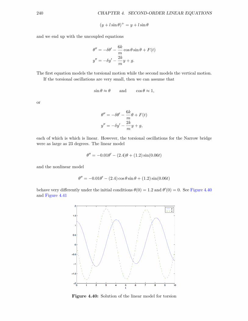
240 CHAPTER 4. SECOND-ORDER LINEAR EQUATIONS
(y + l sin θ)+ = y + l sin θ
and we end up with the uncoupled equations
θ′′ = −δθ′ − 6k
mcos θ sin θ + F (t)
y′′ = −δy′ − 2k
my + g.
The first equation models the torsional motion while the second models the vertical motion.If the torsional oscillations are very small, then we can assume that
sin θ ≈ θ and cos θ ≈ 1,
or
θ′′ = −δθ′ − 6k
mθ + F (t)
y′′ = −δy′ − 2k
my + g,
each of which is which is linear. However, the torsional oscillations for the Narrow bridgewere as large as 23 degrees. The linear model
θ′′ = −0.01θ′ − (2.4)θ + (1.2) sin(0.06t)
and the nonlinear model
θ′′ = −0.01θ′ − (2.4) cos θ sin θ + (1.2) sin(0.06t)
behave very differently under the initial conditions θ(0) = 1.2 and θ′(0) = 0. See Figure 4.40and Figure 4.41
Figure 4.40: Solution of the linear model for torsion

4.4. FORCING AND RESONANCE 241
Figure 4.41: Solution of the nonlinear model for torsion

5
Nonlinear Systems
5.1 LinearizationIn Chapter 3, we explored how to solve linear systems. However, if we are asked to solve anonlinear system such as
dx
dt= x− 3y + xy2
dy
dt= 2x− 4y − x2y,
we are faced with a much more difficult task. In general, it may not be possible to findsolutions for a nonlinear system in terms of elementary functions. However, for a givenmodeling problem, we can ask many questions that may be answered without finding anexplicit solution for the associated system of differential equations. For example, what arethe equilibrium points? Are the equilibrium points stable? Do closed solution curves existin the phase plane?
5.1.1 Equilibrium SolutionsOne of the most useful methods of determining the nature of an equilibrium solution for agiven nonlinear system is to approximate the nonlinear system with a linear system. Morespecifically, an equilibrium solution occurs for the linear system
dx
dt= f(x, y)
dy
dt= g(x, y)
when an x-nullcline intersects a y-nullcline. That is, when a curve defined by dx/dt =f(x, y) = 0 intersects a curve defined dy/dt = g(x, y) = 0, we have an equilibrium solution.Since the x and y-nullclines are simply curves in the xy-plane, we can approximate themlocally by intersecting straight lines. Translating the pair of intersection lines to the origin,we obtain a linear system, and we can apply everything that we learned about such systemsin Chapter 3.
An equilibrium solution for a first-order system of differential equations
x′(t) = f(x, y)
y′(t) = g(x, y)
is a point (x0, y0) such thatf(x0, y0) = g(x0, y0) = 0.
242

5.1. LINEARIZATION 243
Notice that neither x nor y is changing at this point. If we have the initial conditions,x(0) = x0 and y(0) = y0, then the solution to the system is x(t) = x0 and y(t) = y0.Of course the interesting question is what happens if our initial conditions are close to anequilibrium solution. Do solutions tend toward the equilibrium solution, away from theequilibrium solution, or is there a combination of the two?
One of the most useful methods of determining the nature of an equilibrium solutionfor a given nonlinear system is to approximate the nonlinear system with a linear system.More specifically, an equilibrium solution occurs for the linear system
dx
dt= f(x, y)
dy
dt= g(x, y)
when an x-nullcline intersects a y-nullcline. That is, when a curve defined by dx/dt =f(x, y) = 0 intersects a curve defined dy/dt = g(x, y) = 0, we have an equilibrium solution.Since the x and y-nullclines are simply curves in the xy-plane, we can approximate themlocally by intersecting straight lines. Translating the pair of intersection lines to the origin,we obtain a linear system, and we can apply everything that we learned about such systemsin Chapter 3.
Example 5.1. Consider the system
dx
dt= x− 3y + xy2
dy
dt= 2x− 4y − x2y.
From
dx
dt= x− 3y + xy2 = 0
dy
dt= 2x− 4y − x2y = 0,
we can quickly conclude that the only equilibrium solution to the system is (0, 0). The phaseportrait for this system is given in Figure 5.2. If we have the initial conditions x(0) = 1and y(0) = 1, we can see that the solution tends toward the origin as t → ∞. However, itis unclear from the phase portrait if the solution curves of all initial value problems withinitial conditions near the origin tend towards the equilibrium solution as t→ ∞.

244 CHAPTER 5. NONLINEAR SYSTEMS
-2 -1 0 1 2
x(t)
-2
-1
0
1
2
y(t)
Figure 5.2: Phase Portrait for x′ = x− 3y + xy2 and 2x− 4y − x2y
Since the nonlinear terms of the system do not contribute much towards dx/dt anddy/dt for values of x and y near zero, we can determining the nature of the equilibriumsolution by examining the system consisting of only linear terms on the right-hand side ofthe equation,
dx
dt= x− 3y
dy
dt= 2x− 4y.
The matrix for this linear system,
A =
(1 −3
2 −4
),
has eigenvalues λ = −1 and µ = −2 with eigenvectors u = (3, 2) and v = (1, 1), respectively.The general solution for this linear system is
x(t) = 3c1e−t + c2e
−2t
y(t) = 2c1e−t + c2e
−2t.
This indeed suggests that solutions near the origin tend towards the origin as t → ∞. Inthis case, we say that the equilibrium solution is stable. Of course, if we are given an initialcondition such as x(0) = −0.5 and y(0) = 1.
Example 5.3 (A Competing Species Model). Suppose that x and y are the population oftwo distinct species that compete for the same resources. For example, two species of fishmay compete for the same food in a lake or sheep and cattle competing for the same grazingland. Recall from Section 2.2 that we can model two competing species using the followingsystem of first-order differential equations,
dx
dt= αx
(1− x
M
)− βxy

5.1. LINEARIZATION 245
dy
dt= γy
(1− y
N
)− δxy.
The first term in each equation is the logistic growth of each species. The second term ineach equation tells how each species is affected by interacting with the competing species.
More specifically, let us consider the following system,dx
dt= 2x
(1− x
2
)− xy (5.1)
dy
dt= 3y
(1− y
3
)− 2xy. (5.2)
It is easy to see that the four equilibrium solutions: (0, 0), (0, 3), (2, 0), and (1, 1). Wecan view the direction field, the phase plane, and some solution curves for this system inFigure 5.4.
0 1 2 3 4
x(t)
0
1
2
3
4
y(t)
Figure 5.4: A Competing Species Model
Let us analyze what happens at the equilibrium solution (1, 1). If we decide on anappropriate change of variables, we can translate the entire system so that this equilibriumsolution is at the origin. If we let
u = x− 1
v = y − 1,
thendu
dt=
d
dt(x− 1) =
dx
dt,
dv
dt=
d
dt(y − 1) =
dy
dt.
Equations (5.1) and (5.2) now becomedu
dt= −u− v − u2 − uv, (5.3)

246 CHAPTER 5. NONLINEAR SYSTEMS
dv
dt= −2u− v − 2uv − v2. (5.4)
As before we consider only the linear part of equations (5.4) and (5.4) aredu
dt= −u− v, (5.5)
dv
dt= −2u− v. (5.6)
The idea is that the linear part is a good local approximation to the original equationsmuch like a tangent line is a good local approximation to a smooth function in calculus. Wecan determine the local nature of the equilibrium solution by examining the eigenvalues ofthe matrix
A =
(−1 −1
−2 −1
).
The eigenvalues of A are λ = −1 +√2 = 0.4142 and µ = −1 −
√2 ≈ −2.4142 with
eigenvectors u = (1,√2 ) ≈ (1, 1.4142) and v = (1,−
√2 ) ≈ (1,−1.4142), respectively. The
solution to the linear system is now
x(t) = c1eλt
(1√2
)+ c2e
µt
(1
−√2
).
or
x(t) = c1eλt + c2e
µt (5.7)y(t) = c1
√2eλt − c2
√2eµt. (5.8)
If we have initial conditions x(0) = 3 and y(0) = 4, one can quickly determine thatc1 = 3/2+
√2 ≈ 2.9142 and c2 = 3/2−
√2 ≈ 0.0859, and equations (5.7) and (5.8) become
x(t) = 2.9142e0.4142t + 0.0859e−2.4142t (5.9)y(t) = 4.1213e0.4142t − 0.1213e−2.4142t. (5.10)
As t→ ∞ notice that both x(t) and y(t) become very large and tend away from the origin.We can conclude that the equilibrium solution (1, 1) is unstable. That is, tend away
from the equilibrium solution as t → ∞ if one population begins with a slight advantageover the other. If neither popluation has an initial advantage over the other, then thesolution curve will approach the equilibrium solution as t→ ∞.Example 5.5 (A Nonpolynomial Example). If systems such as the following can be ap-proximated by linear systems,
dx
dt= y
dy
dt= −y − sinx.
Certainly, this sytems has an equilibrium solution at (0, 0). We can expand sinx into apower series,
dy
dt= −y − sinx = −y −
(x− x3
3!+x5
5!− · · ·
).
Thus, this system can be approximated by the linear systemdx
dt= y
dy
dt= −y − x.

5.1. LINEARIZATION 247
-4 -2 0 2 4
x(t)
-4
-2
0
2
4
y(t)
Figure 5.6: Phase portrait of x′ = y and y′ = −y − sinx
-4 -2 0 2 4
x(t)
-4
-2
0
2
4
y(t)
Figure 5.7: Phase portrait of x′ = y and y′ = −y − x
Example 5.8. For example, consider the system
dx
dt= x2 − 4x− y + 4 (5.11)
dy
dt= x3 − y. (5.12)

248 CHAPTER 5. NONLINEAR SYSTEMS
The x and y-nullclines of this system are the curves y = x2−4x+4 and y = x3, respectively.Since the two nullclines intersect only at (1, 1), we have a single equilibrium solution. Fromthe phase plane, it appears that (1, 1) is a stable equilibrium solution. That is, all solutioncurves starting sufficiently close to (1, 1) will approach the equilibrium solution as t → ∞(Figure 5.9).
-1 0 1 2 3
x(t)
-1
0
1
2
3
y(t)
Figure 5.9: Phase portrait for the system (5.11)–(5.12)
Making the substitution u = x − 1 and v = y − 1, simply translates the entire systemto the origin, and we obtain the system
du
dt= u(u− 2)− v (5.13)
dv
dtu(u2 + 3u+ 3)− v. (5.14)
Our new system has u and v-nullclines v = u(u − 2) and v = u(u2 + 3u + 3), respectively.Notice that we have simply moved the phase portrait of the original system so that ourequilibrium solution is now at the origin. Furthermore, we can approximate the u andv-nullclines by their tangent lines v = −2u and v = 3u, respectively. From Figure 5.9, itappears that we are approximating our original system with a linear system.

5.1. LINEARIZATION 249
-2 -1 0 1 2
u(t)
-2
-1
0
1
2
v(t)
Figure 5.10: Phase portrait for the system (5.13)–(5.14)
To determine the general case, we must approximate a nonlinear system
x′(t) = f(x, y) (5.15)y′(t) = g(x, y) (5.16)
near each equilibrium point (x0, y0) with a linear system. The idea is to move the equilibriumsolution to the origin with a change of coordinates and then approximate the nonlinearsystem with a linear system. In order to move the equilibrium solution to the origin, wewill introduce new variables
u = x− x0
v = y − y0.
If (x, y) is close to the equilibrium solution (x0, y0), then (u, v) will be close to the origin.Under this change of coordinates,
du
dt=
d
dt(x− x0) =
dx
dt= f(x, y) = f(x0 + u, y0 + v).
Similarly, dv/dt = dy/dt = g(x0 + u, y0 + v).In order to approximate the nonlinear system with a linear system, we will use a Taylor
series in two variables. That is, we can write
f(x0 + u, y0 + v) = f(x0, y0) + fx(x0, y0)u+ fy(x0, y0)v
+1
2fxx(x0, y0)u
2 + fxy(x0, y0)uv +1
2fyy(x0, y0)v
2 + · · · .
If we only use the linear terms of the Taylor series, we obtain a fairly accurate approximationof f provided we are near the equilibrium solution. Of course, f and its linear approximation

250 CHAPTER 5. NONLINEAR SYSTEMS
may be quite different for values far away from the equilibrium solution. The linearizationof the system of equations (5.15)–(5.16) now becomes
du
dt= f(x0, y0) + fx(x0, y0)u+ fy(x0, y0)v
dv
dt= g(x0, y0) + gx(x0, y0)u+ gy(x0, y0)v.
Since (x0, y0) is an equilibrium solution, the constant terms vanish in each equation and
du
dt= fx(x0, y0)u+ fy(x0, y0)v
dv
dt= gx(x0, y0)u+ gy(x0, y0)v.
If we write our linearization in matrix form, we have(du/dt
dv/dt
)=
(fx(x0, y0) fy(x0, y0)
gx(x0, y0) gy(x0, y0)
)(u
v
).
The matrix
J =
(fx(x0, y0) fy(x0, y0)
gx(x0, y0) gy(x0, y0)
)is the Jacobian matrix of the system. We can now classify equilibrium solutions ofnonlinear systems by examining the eigenvalues of the Jacobian matrix of the system or byusing the trace-determinant plane. For example, if D = det(J) > 0 and T = tr(J) < 0, wehave a sink. We can determine the sink to be spiral or nodal by examining whether (T,D)lies above or below the parabola T 2 = 4D in the trace-determinant plane.
It is important to note that linearization only tells us the local story. A solution curvemight behave quite differently if it is far away from the equilibrium solution.
Example 5.11. In Example 5.8, we considered the system
dx
dt= x2 − 4x− y + 4
dy
dt= x3 − y.
The Jacobian matrix of this system is
J =
(fx(x0, y0) fy(x0, y0)
gx(x0, y0) gy(x0, y0)
)=
(2x0 − 4 −1
3x20 −1
)For the equilibrium solution (1, 1),
J =
(−2 −1
3 −1
).
Since J has eigenvalues λ = (−3 ± i√11)/2, the equilibrium solution will act as a spiral
sink for initial values close to (1, 1).

5.1. LINEARIZATION 251
5.1.2 When Linearization Fails
There are at least two cases when linearization does not give us the information that weseek. First, it might well be the case that the linear terms vanish in the nonlinear system.For example, the system
dx
dt= xy
dy
dt= −x2 + xy
has an equilibrium solution at the origin, but this linearization of this system vanishes.A more subtle example is the system
dx
dt= y − (x2 + y2)x
dy
dt= −x− (x2 + y2)y.
The origin is an equilibrium solution, and the linearization of this system is
dx
dt= y
dy
dt= −x.
The eigenvalue of the matrix corresponding to the linear system,
A =
(0 1
−1 0
),
are λ = ±i. Thus, the solution curves of the linear system are simply circles about theorigin. However, the nonlinear system acts quite differently. In the nonlinear system,solutions spiral out slowly from the origin (Figure 5.12). This system has no periodicsolutions.
-0.2 -0.1 0 0.1 0.2
x(t)
-0.2
-0.1
0
0.1
0.2
y(t)
Figure 5.12: When linearization fails

252 CHAPTER 5. NONLINEAR SYSTEMS
5.1.3 Important Lessons
• We can approximate a nonlinear system
x′(t) = f(x, y)
y′(t) = g(x, y)
near each equilibrium point (x0, y0) with a linear system by using a Taylor seriesapproximation for f and g. The matrix of our linear approximation,
J =
(fx(x0, y0) fy(x0, y0)
gx(x0, y0) gy(x0, y0)
),
is the Jacobian matrix of the system. We can classify nonlinear systems by exam-ining the Jacobian matrix of the system and using the trace-determinant plane.
• Linearization only tells us how solutions behave near the equilibrium point. A solutioncurve might behave quite differently if it is far away from the equilibrium solution.
• In some cases, linearization can fail.
5.1.4 Exercises
1. Consider the following three systems
(a)
x′ = 3 sinx+ y
y′ = 4x+ cos y − 1
(b)
x′ = −3 sinx+ y
y′ = 4x+ cos y − 1
(c)
x′ = −3 sinx+ y
y′ = 4x+ 3 cos y − 3
All three systems have an equilibrium solution at (0, 0). Which two systems have phaseportraits with the same “local picture” near (0, 0)? Justify your answer.
2. Let us consider an epidemic model for a city. We make the following additional assump-tions about our model.
• The city has a constant birth rate rate of α persons per day. All new born babies aresusceptible to the disease.
• Infected people either recover or die after a certain number of days. If an individualrecovers, he or she is immune.

5.1. LINEARIZATION 253
If we let S(t) be the number of susceptible individuals at time t and I(t) be the number ofinfected individuals at time t, our assumptions give rise to the following system of differentialequations,
dS
dt= −αSI + β
dI
dt= −γI + αSI.
The constant α is determined by the probability of an interaction between a susceptibleindividual and an infected individual, and γ is the rate at which infected individuals areremoved from the population. If
dS
dt= −αSI + β = 0
dI
dt= −γI + αSI = 0,
then both the susceptible and infected populations do not change. This will occur at
S0 =γ
α
I0 =β
γ.
We are interested in the behavior of solutions near (S0, I0). If solutions approach thisequilbrium point, then the disease will become endemic to the population.
5.1.5 Project—Modeling the Nervous System
Hodgkin and Huxley developed a model for the firing of nerve cells in the 1950s. The modelwas a system of four differential equations that described the electrochemical transmissionof neuronal signals along cell membranes in giant squid. The system itself was very difficultto analyze due to its highly nonlinear nature, but it did earn the two scientists a NobelPrize for medicine in 1963 (the year after Watson and Crick won their prize).
Fitzhugh and Nagumo managed to simplify the Hodgkin-Huxley model to two equations
x′ = y + x− x3/3 + I
y′ = −x+ a− by,
where a and b are constants satisfying a certain condition and I is a parameter. In theseequations, x represents the excitability of the system and y represents a combination ofother forces that return the system to rest. Similar models have been constructed to modelthe systolic and diastolic movements of the heart.
We will now consider the system
dx
dt= x+ y − x3
dy
dt= −0.5x,
which has been used to study nerve cells and is similar to the Fitzhugh-Nagumo model.The x-nullcline for this system is y = −x + x3. The x-component of the direction field

254 CHAPTER 5. NONLINEAR SYSTEMS
above this nullcline is positive. Below the nullcline the x-component of the direction fieldis negative.
The y-nullcline of the system is the y-axis. To the right of the y-nullcline, we havedy/dt < 0, and dy/dt > 0 to the left of the y-nullcline. Thus, the x and y-nullclines dividethe plane into four regions and all solutions must circulate in a clockwise manner about theorigin (Figure 5.13).
-2 -1 0 1 2
x(t)
-2
-1
0
1
2
y(t)
Figure 5.13: Modeling nerve cells
The origin is the only equilibrium solution of the system; hence, we can examine thelinearization
dx
dt= x+ y
dy
dt= −0.5x,
to determine the nature of the equilibrium solution. Since the eigenvalues of this linearsystem are (1 ± i)/2, we can conclude that the origin is a spiral source. A solution thatpasses close to the origin tends to spiral outward; however, solutions that are far from theorigin spiral inward. We shall later see that we must have a closed periodic solution to thissystem by the Poincaré-Bendixson Theorem.
5.2 Hamiltonian Systems
An undamped harmonic oscillator, my′′ + ky = 0, can be written as the system
y′ = v
v′ = − k
my.

5.2. HAMILTONIAN SYSTEMS 255
Now suppose that (y(t), v(t)) is a solution curve in the yv-plane. We will calculate the slopeof the solution curve, dv/dy. Using the fact from calculus that the derivative of an inversefunction is
d
dxf−1(x) =
1
f ′(x),
we havedv
dy=dv
dt· dtdy
=dv/dt
dy/dt= − ky
mv.
In general for the system
dx
dt= f(x, y)
dy
dt= g(x, y),
we havedy
dx=g(x, y)
f(x, y).
Using separation of variables to solve the equation
dv
dy= − ky
mv,
we obtain the solution1
2mv2 +
1
2ky2 = C, (5.17)
where C is a constant. The first term of (5.17) is the kinetic energy function of theharmonic oscillator
K =1
2mv2,
while the second term is the potential energy function
U =
∫ y
0ks ds =
1
2ky2.
For this reason, we call the function
E = K + U =1
2mv2 +
1
2ky2
the total energy function of the harmonic oscillator. Equation (5.17) tells us that energyis conserved. That is, the sum of the potential energy and the kinetic energy is constant.
5.2.1 The Nonlinear Pendulum
While pendulums have long been used in clocks to keep time, they have also been used tomeasure gravity as well as used in early seismometers to measure the effect of earthquakes.One of the more interesting uses of a pendulum has been to measure the rotation of theearth. In 1851, the French physicist, Léon Foucault, used a pendulum (Figure 5.14) todemonstrate that the earth actually rotated on its axis. The fact that the earth rotates hadbeen known for a long time, but Foucault’s experiment give the first simple proof of thisphenomena.

256 CHAPTER 5. NONLINEAR SYSTEMS
Figure 5.14: Foucault Pendulum Clock—California Academy of Sciences
Let us consider a pendulum made of a light rod of length L called the arm of thependulum with a mass mon the end of the rod called the bob (Figure 5.15). We will ignorethe mass of the arm in our system. The position of the bob is given by θ(t), which we willmeasure in a counterclockwise direction. We will assume that θ(0) is when the bob is inthe vertical position.
m
Lθ
Figure 5.15: The nonlinear pendulum
There are two forces acting on the pendulum—gravity and friction. The position of thebob at time t is
(L sin θ(t),−L cos θ(t)),and the velocity of the bob is L(dθ/dt), the length of the velocity vector (Figure 5.16) Thecomponent of the acceleration that points along the direction of motion of the bob is
Ld2θ
dt2.
We can take the force due to friction to be proportional to the velocity,
−bLdθdt,
where b ≥ 0. Thus, Newton’s second law tells us that
mLd2θ
dt2= −bLdθ
dt−mg sin θ
ord2θ
dt2+
b
m
dθ
dt+g
Lsin θ = 0.

5.2. HAMILTONIAN SYSTEMS 257
As a system, we can model the pendulum as
dθ
dt= v
dv
dt= − b
mv − g
Lsin θ.
Lθ
mg sin θ
mg
Figure 5.16: Forces on the nonlinear pendulum
If there is no damping for our pendulum, we say that we have an ideal pendulum. Inthis case,
dθ
dt= v
dv
dt= − g
Lsin θ.
Sincedv
dθ= −g sin θ
Lv,
we know that the energy function for the pendulum is
E(θ, v) =1
2v2 − g
Lcos θ.
Of course, E(θ, v) is constant on the ideal pendulum.
5.2.2 Hamiltonian SystemsThe ideal pendulum and the undamped harmonic oscillator are examples of Hamiltoniansystems. More specifically, a Hamiltonian system is a system of the form
dx
dt=∂H
∂y(x, y)
dy
dt= −∂H
∂x(x, y),
where H : R2 → R is a smooth function.
Example 5.17. The system
dx
dt= −2x− 3y2
dy
dt= −3x2 + 2y

258 CHAPTER 5. NONLINEAR SYSTEMS
is Hamiltonian since for H(x, y) = x3 − 2xy − y3
∂H
∂y= −2x− 3y2
∂H
∂x= −(−3x2 + 2y).
Example 5.18. In the case of the harmonic oscillator and ideal pendulum, H is just theenergy function. For the harmonic oscillator, the Hamiltonian function is
E = K + U =1
2mv2 +
1
2ky2.
In this case,
∂E
∂v= y′ = mv
−∂E∂y
= v′ = −ky.
A change of variables (y = my) tells us that this system is equivalent to the system
y′ = v
v′ = − k
my.
For the ideal pendulum
∂E
∂v=dθ
dt= v
−∂E∂θ
=dv
dt= − g
Lsin θ,
whereE(θ, v) =
1
2v2 − g
Lcos θ.
The following theorem tells the the importance of Hamiltonian systems. That is, thesolution curves of the system are simply the level sets of the Hamiltonian function.
Theorem 5.19. Let
dx
dt=∂H
∂y(x, y)
dy
dt= −∂H
∂x(x, y),
be a Hamiltonian system, where H : R2 → R. Then H is constant along any solution curve.
Proof. Let (x(t), y(t)) be a solution curve for the system. Using the chain rule
dH
dt=∂H
∂x
dx
dt+∂H
∂y
dy
dt
=∂H
∂x
(∂H
∂y
)+∂H
∂y
(−∂H∂x
)= 0.

5.2. HAMILTONIAN SYSTEMS 259
Theorem 5.19 tells us how to draw the solution curves in the phase plane without solvingthe system. Assuming that the Hamiltonian function H is not constant on any open setin R2, we simply need to plot the level curves, H(x, y) = C. The solutions of the systemlive on these level sets, and all we need to do is find the direction of the solution curve.However, this is quite easy since we know the vector field of the system. Furthermore, theequilibrium points of the Hamiltonian system occur at the critical points of H (where thepartials of H vanish). For example, we can see the solution curves of
∂H
∂y= −2x− 3y2
∂H
∂x= −(−3x2 + 2y).
in Figure 5.20.
-1.5 -1 -0.5 0 0.5 1 1.5
x(t)
-1.5
-1
-0.5
0
0.5
1
1.5
y(t)
Figure 5.20: Solution curves of x′ = x− 3y2 and y′ = −y
5.2.3 The Ideal Pendulum RevisitedThe ideal pendulum
dθ
dt= v
dv
dt= − g
Lsin θ.
is Hamiltonian, since the total energy function
H(θ, v) = E(θ, v) =1
2v2 − g
Lcos θ. (5.18)
is the Hamiltonian function for the system. If we set g/L = 1, then the solution curves ofthe system are just the level curves of (5.18). In Figure 5.21, the closed ellipses correspondto the normal motion of a pendulum, while cosine curves correspond to a pendulum that

260 CHAPTER 5. NONLINEAR SYSTEMS
always rotates in the same direction. The curves that join the equilibrium points correspondto the pendulum that rotates exactly to the top of the arc and then rotates back in theother direction.
−4π −3π −2π −π 0 π 2π 3π 4π
θ(t)
−4
−3
−2
−1
0
1
2
3
4
v(t)
Figure 5.21: The ideal pendulum
Hamiltonian systems are rather rare. Given a system, we need a test to see if it is indeedHamiltonian. For the system
dx
dt= f(x, y)
dy
dt= g(x, y),
we wish to find a function H(x, y) such that
∂H
∂y= f(x, y)
∂H
∂x= −g(x, y).
If such a function exists, then
∂f
∂x=
∂2H
∂x∂y=
∂2H
∂y∂x= −∂g
∂y.
Thus,∂f
∂x= −∂g
∂y,
if our system is Hamiltonian.
Example 5.22. We already know that the system
dx
dt= −2x− 3y2
dy
dt= −3x2 + 2y
is Hamiltonian. Indeed,∂f
∂x= −∂g
∂y= −2.

5.2. HAMILTONIAN SYSTEMS 261
The condition that∂f
∂x= −∂g
∂y,
is also sufficient for
dx
dt= f(x, y)
dy
dt= g(x, y),
to be a Hamiltonian system. That is, we can construct a Hamiltonian function if ∂f/∂x =−∂g/∂y. If
f(x, y) =∂H
∂y(x, y),
thenH(x, y) =
∫f(x, y) dy + ϕ(x).
Differentiating H with respect to x, tells us that
∂H
∂x(x, y) =
∂
∂x
∫f(x, y) dy + ϕ′(x) = −g(x, y).
Now we can determine ϕ(x) by solving the first-order differential equation
ϕ′(x) = −g(x, y)− ∂
∂x
∫f(x, y) dy.
We summarize our results in the following theorem.
Theorem 5.23. Let
dx
dt= f(x, y)
dy
dt= g(x, y),
where f and g are continuously differentiable.
1. If the system is Hamiltonian, then
∂f
∂x= −∂g
∂y. (5.19)
2. If equation (5.19) is true on a rectangle R, then the system is Hamiltonian on R and
H(x, y) =
∫f(x, y) dy + ϕ(x),
whereϕ′(x) = − ∂
∂x
(∫f(x, y) dy
)− g(x, y).
Example 5.24. As an example, we will show how we constructed the Hamiltonian functiongiven in Example 5.17 for the system
dx
dt= −2x− 3y2

262 CHAPTER 5. NONLINEAR SYSTEMS
dy
dt= −3x2 + 2y
First,
H(x, y) =
∫f(x, y) dy + ϕ(x) =
∫(−2x− 3y2) dy + ϕ(x) = −2xy − y3 + ϕ(x).
Consequently,
ϕ′(x) = −g(x, y)− ∂
∂x
∫f(x, y) dy
= −(−3x2 + 2y)− ∂
∂x(−2xy − y3)
= 3x2 − 2y + 2y
= 3x2,
and ϕ(x) = x3+C, where C is any constant. If we choose C = 0, our Hamiltonian functionis
H(x, y) = −2xy − y3 + ϕ(x) = −2xy − y3 + x3.
Example 5.25. As a second example, suppose
dx
dt= −x2 cos y sinx
dy
dt= x2 cosx sin y + 2x(sinx sin y − 1).
Since∂f
∂x= x2 cosx cos y − 2x cos y sinx = −∂g
∂y
our system is Hamiltonian. To find a Hamiltonian, we compute
H(x, y) =
∫f(x, y) dy + ϕ(x) =
∫(−x2 cos y sinx) dy + ϕ(x) = −x2 sinx sin y + ϕ(x).
Thus,
ϕ′(x) = −g(x, y)− ∂
∂x
∫f(x, y) dy
= −(x2 cosx sin y + 2x(sinx sin y − 1))− (2x sinx sin y − x2 cosx sin y)= 2x,
and ϕ(x) = x2 + C. Letting C = 0, our Hamiltonian function is
H(x, y) = x2 − x2 sinx sin y = x2(1− sinx sin y).
Solution curves for this system are given in Figure 5.26.

5.2. HAMILTONIAN SYSTEMS 263
-6 -4 -2 0 2 4 6
x(t)
-6
-4
-2
0
2
4
6
y(t)
Figure 5.26: Solution curves for Example 5.25
5.2.4 Equilibrium Solutions of Hamiltonian SystemsThe system that we studied in Example 5.17,
dx
dt= −2x− 3y2
dy
dt= −3x2 + 2y
has equilibrium solutions at (0, 0) and (−2/3, 2/3). Referring to the phase portrait for thesystem (Figure 5.20), we might guess that (0, 0) is a saddle and (−2/3.2/3) is either a centeror a spiral sink. Since solution curves must follow contours for the Hamiltonian functionH(x, y) = x3 − 2xy − y3, spiral sinks do not make sense.
Let us examine the possible types of equilibrium solutions for a Hamiltonian system.Suppose that (x0, y0) is an equilibrium solution for the system
dx
dt= f(x, y) =
∂H
∂y(x, y)
dy
dt= g(x, y) = −∂H
∂x(x, y).
In order to determine the nature of the equilibrium solution, we will compute the Jacobianmatrix of the system at (x0, y0),
J =
(fx(x0, y0) fy(x0, y0)
gx(x0, y0) gy(x0, y0)
)=
(Hyx(x0, y0) Hyy(x0, y0)
−Hxx(x0, y0) −Hxy(x0, y0)
).
If we let
α = Hxy(x0, y0) = Hyx(x0, y0)
β = Hyy(x0, y0)

264 CHAPTER 5. NONLINEAR SYSTEMS
γ = −Hxx(x0, y0),
then J becomes (α β
γ −α
).
The characteristic polynomial of this matrix is
λ2 − α2 − βγ.
Therefore, our matrix has eigenvalues
λ = ±√α2 + βγ,
and we have the following possibilities.
• If α2 + βγ > 0, we have two real eigenvalues of opposite signs. Therefore, our equi-librium solution is a saddle.
• If α2 + βγ = 0, the only eigenvalue is zero.
• If α2 + βγ < 0, we have two purely imaginary eigenvalues.
In particular, a Hamiltonian system has no spiral sinks or sources.Returning to Example 5.17, the Jacobian matrix is
J =
(Hyx(x0, y0) Hyy(x0, y0)
−Hxx(x0, y0) −Hxy(x0, y0)
). =
(−2 −6y0
−6x0 2
).
For the equilibrium solution (0, 0), we have eigenvalues λ = ±2, which tells us that theorigin is a nodal saddle. The Jacobian matrix corresponding to (x0, y0) = (−2/3, 2/3) is
J =
(−2 −4
−4 2
).
Since J has eigenvalues λ = ±2√5 i. Therefore, solution curves near (−2/3, 2/3) should
look like closed orbits.
5.2.5 Important Lessons
• A pendulum can be modeled by the equation
d2θ
dt2+
b
m
dθ
dt− g
Lsin θ = 0.
or the systemdθ
dt= v
dv
dt= − b
mv − g
Lsin θ.
• A Hamiltonian system is a system of the formdx
dt=∂H
∂y(x, y)
dy
dt= −∂H
∂x(x, y),
where H : R2 → R2 is a smooth function.

5.2. HAMILTONIAN SYSTEMS 265
• If
dx
dt=∂H
∂y(x, y)
dy
dt= −∂H
∂x(x, y),
is a Hamiltonian system, then H is constant along any solution curve. In particular,the solution curves of a Hamiltonian system are the level sets of H.
• If the system
dx
dt= f(x, y)
dy
dt= g(x, y),
is Hamiltonian, then∂f
∂x= −∂g
∂y.
• If fx = −gy is true on a rectangle R, then the system
dx
dt= f(x, y)
dy
dt= g(x, y),
is Hamiltonian on R and
H(x, y) =
∫f(x, y) dy + ϕ(x),
whereϕ′(x) = − ∂
∂x
(∫f(x, y) dy
)− g(x, y).
• A Hamiltonian system has no spiral sinks or sources.
5.2.6 Exercises1. Consider an ideal pendulum with bob mass m and arm length l given by
dθ
dtv
dv
dt− g
lsin θ.
(a) What is the linearization of the ideal pendulum system at the equilibrium point (0, 0)?(b) Using g = 9.8 m/s2, how should l andm be chosen so that small swings of the pendulum
have period 1 second?(c) For the linearization of the ideal pendulum at (0, 0), the period of oscillation is in-
dependent of the amplitude. Does the same statement hold for the ideal pendulumitself? Is the period of oscillation the same no matter how high the pendulum swings?If not, will the period be shorter or longer for high swings?

266 CHAPTER 5. NONLINEAR SYSTEMS
(d) An ideal pendulum clock— a clock containing an ideal pendulum that “ticks” once foreach swing of the pendulum arm— keeps perfect time when the pendulum makes veryhigh swings. Will the clock rum fast or slow if the amplitude of the swings is verysmall?
(e) If the arm length of the ideal pendulum is doubled from l to 2l, what is the effect onthe period of small amplitude swinging solutions?
(f) What is the rate of change of the period of small amplitude swings as l varies?(g) Will an ideal pendulum clock that keeps perfect time on earth run fast or slow on the
moon?
2. Describe the phase portrait for
x′x2 − 1
y′ − xy + a(x2 − 1),
when a < 0.
3. Consider the autonomous system
x′y2 + cosxy′1 + 2x+ y sinx.
(a) Show that this system is a Hamiltonian system.(b) Find a Hamiltonian function for this system.
5.2.7 ProjectsPossible project
5.3 More Nonlinear MechanicsThe equation for the nonlinear pendulum with damping is
d2θ
dt2+
b
m
dθ
dt+g
Lsin θ = 0.
As a system, we can model the pendulum as
dθ
dt= v (5.20)
dv
dt= − b
mv − g
Lsin θ. (5.21)
This system is not Hamiltonian since
∂v
∂θ= 0,
but− ∂
∂v
(− b
mv − g
Lsin θ
)=
b
m= 0.
We shall have to invent new techniques to analyze such systems.

5.3. MORE NONLINEAR MECHANICS 267
5.3.1 The Nonlinear Pendulum and DampingTo find the nullclines of the nonlinear pendulum, let
dθ
dt= v = 0
dv
dt= − b
mv − g
Lsin θ = 0.
The θ-nullcline is v = 0, while the v-nullcline is
v = −mgbL
sin θ.
It follows that the equilibrium solutions for the nonlinear pendulum occur at
(θ, v) = (0, 0), (±π, 0), (±2π, 0), . . . .
This makes sense since the pendulum should not move if the bob is initially hanging down-ward (θ = 2πn) or is at the very top or the very bottom of a swing (θ = (2n+ 1)π). Sinceour first goal is to determine the nature of each equilibrium solution, we will compute theJacobian of the system (5.20)–(5.21). This is just(
0 1
−(g/L) cos θ −b/m
).
At the equilibrium solutions (θ, v) = (0, 0), (±2π, 0), (±4π, 0), . . ., the pendulum is hangingdownward, and the Jacobian matrix becomes
J1 =
(0 1
−g/L −b/m
).
On the other hand, if (θ, v) = (±π, 0), (±3π, 0), (±5π, 0), . . ., the pendulum is at the top ofits swing, and the Jacobian matrix is
J2 =
(0 1
g/L −b/m
).
We will first examine the case where the pendulum is hanging downward. The charac-teristic polynomial of J1 is
λ2 +b
mλ+
g
L.
Thus, the eigenvalues of J1 are
λ = − b
2m±
√(b
2m
)2
− g
L. (5.22)
We can analyze the nature of these eigenvalues by examining the sign of
∆ =
(b
2m
)2
− g
L.
• If ∆ < 0, the eigenvalues of the Jacobian are complex. Since the real part of (5.22) isnegative, these equilibrium solutions are spiral sinks.

268 CHAPTER 5. NONLINEAR SYSTEMS
• If ∆ > 0, we have two distinct real eigenvalues. Since(b
2m
)2
− g
L<
(b
2m
)2
,
we know that (b
2m
)>
√(b
2m
)2
− g
L.
Thus, both of our eigenvalues must be negative. Therefore, we have a nodal sink.
• If ∆ = 0, we have a single real negative eigenvalue. Thus, we also have a sink.
Consequently, if we assume that b is small, then ∆ < 0 and we will only have spiral sinks(Figure 5.27).
−3π −2π −π 0 π 2π 3π
θ(t)
−4
−3
−2
−1
0
1
2
3
4
v(t)
Figure 5.27: Nullclines of the damped pendulum
Now let us consider the type of equilibrium solutions that we will obtain when the pendu-lum is standing upright. These solutions will occur at (θ, v) = (±π, 0), (±3π, 0), (±5π, 0), . . ..The characteristic polynomial of the Jacobian matrix J2 at these points is
λ2 +b
mλ− g
L;
hence, the eigenvalues of J2 are
λ = − b
2m±
√(b
2m
)2
+g
L. (5.23)
Furthermore, we have distinct real eigenvalues since(b
2m
)2
+g
L> 0.
In fact, the eigenvalues will have opposite sign
λ1 = − b
2m+
√(b
2m
)2
+g
L> 0

5.3. MORE NONLINEAR MECHANICS 269
λ2 = − b
2m−
√(b
2m
)2
+g
L< 0.
Thus, the equilibrium solutions are saddles.
5.3.2 Lyapunov FunctionsThe function
H(θ, v) =1
2v2 − g
Lcos θ
is a Hamiltonian function for the ideal pendulum
dθ
dt= v
dv
dt= − g
Lsin θ,
since dH/dt = 0. However, if b > 0, then our system
dθ
dt= v
dv
dt= − b
mv − g
Lsin θ.
has damping and
dH
dt=∂H
∂θ
dθ
dt+∂H
∂v
dv
dt
=( gL
sin θ)v + v
(− b
mv − g
Lsin θ
)= − b
mv2 ≤ 0.
Thus, H is decreasing whenever v = 0. Hence solution curves in the θv-plane cross the levelsets of H moving from larger to smaller H values.
We can now devise a strategy for sketching the phase plane of the damped pendulum. Ifb/m and v are both small, the value of H decreases slowly along the solutions (Figure 5.27).
The function H in the case of the damped pendulum is an example of a Lyapunovfunction. Specifically, a function L(x, y) is called a Lyapunov function for the system
dx
dt= f(x, y)
dy
dt= g(x, y)
if for every solution of the system, (x(t), y(t)), that is not an equilibrium solution of thesystem,
dL
dt≤ 0,
with strict inequality except possible for a discrete set of ts.As an example, let us return to the damped harmonic oscillator
dy
dt= v
dv
dt= −qy − pv.

270 CHAPTER 5. NONLINEAR SYSTEMS
If p = 0, then
H(y, v) =1
2v2 +
q
2y2
is a Hamiltonian function for our system. Recall that we also call H the energy function ofthe system. However, if p > 0 and (y(t), v(t)) is a solution for our system, we have
dH
dt(y, v) =
∂H
∂y
dy
dt+∂H
∂v
dy
dt
= (qy)v + v(−qy − pv)
= −pv2 ≤ 0.
Consequently, H(y(t), v(t)) decreases at a nonzero rate (except when v = 0), and H is aLyapunov function. The level sets of H are ellipses in the yv-plane. As H decreases, theenergy dissipates and the ellipses become spiral sinks.
It is easy to see that the system
dx
dt= y + αx(x2 + y2) (5.24)
dy
dt= −x+ αy(x2 + y2) (5.25)
has an equilibrium solution at the origin no matter what the value of α is. The Jacobianof this system is
J =
(3αx2 + αy2 1 + 2αxy
−1 + 2αxy αx2 + 3αy2
).
Since our equilibrium solution is the origin,
J =
(0 1
−1 0
)
and the linearization of our system at the origin is
dx
dt= y
dy
dt= −x.
Since the eigenvalues of
J =
(0 1
−1 0
),
are ±i, the linearization has a center at the origin. The phase plane consists of circles aboutthe origin (Figure 5.28). Notice that the linearization does not depend on α.

5.3. MORE NONLINEAR MECHANICS 271
-3 -2 -1 0 1 2 3
x(t)
-3
-2
-1
0
1
2
3
y(t)
Figure 5.28: Solution curves for the linearization.
Now let us consider what happens to system (5.24)–(5.25) if we consider different valuesof α. If α = 5, the situation is quite different that the linearization of our system. Asolution curve spirals out from the origin as t→ ∞ (Figure 5.29). As t→ −∞, the solutioncurve spirals back into the origin, but it seems to stop before actually reaching the origin. Ifα = −5 on the other hand, we seem to have the opposite behavior with the solution curvesspiraling into the origin as t→ ∞. As before, the solutions do not seem to reach the origin(Figure 5.30).

272 CHAPTER 5. NONLINEAR SYSTEMS
-3 -2 -1 0 1 2 3
x(t)
-3
-2
-1
0
1
2
3
y(t)
Figure 5.29: Solution curves α = 5.
-3 -2 -1 0 1 2 3
x(t)
-3
-2
-1
0
1
2
3
y(t)
Figure 5.30: Solution curves for α = −5.
Suppose that (x(t), y(t)) is a solution to the nonlinear system. The function
r(t) =√x(t)2 + y(t)2
is the distance of a point on the solution curve to the origin in the xy-plane. To see how rchanges as t→ ±∞, we can compute the derivative of r. Actually, it is easier to work with

5.3. MORE NONLINEAR MECHANICS 273
the equation r(t)2 = x(t)2 + y(t)2. Thus,
d
dtr2 =
d
dt(x(t)2 + y(t)2)
= 2xdx
dt+ 2y
dy
dt= 2x(y + αx(x2 + y2)) + 2y(−x+ αy(x2 + y2))
= 2α(x2 + y2)2
= 2αr4.
Since (r2)′ = 2rr′, we haver′ = αr3 (5.26)
for r = 0.Equation (5.26) is separable, and it is quite easy to determine the solution as
r(t) =1√
C − 2αt.
However, we do not need to know this solution to determine the nature of the equilibriumsolution at the origin. If α > 0 and t → −∞, equation (5.26) tells us that r(t) → 0. Thus,any solution to the system (5.24)–(5.25) we have a spiral sink at the origin if α = −5. Eventhough linearization fails to tell us the nature of the equilibrium solution at the origin, wewere able to determine the nature of the equilibrium solution with further analysis.
We will now try to exploit what we have learned from our last example and fromHamiltonian systems to see if it is possible to analyze more general systems. If we considersolutions, (x(t), y(t)), of the system
dx
dt= f(x, y)
dy
dt= g(x, y),
we might ask how a function V (x, y) varies along the solution curve. We already have ananswer if our system is Hamiltonian, and V is the corresponding Hamiltonian function. Inthis case dV /dt = 0. In general, we know that
dV
dt(x(t), y(t)) =
∂V
∂x
dx
dt+∂V
∂y
dy
dt
=∂V
∂xf(x, y) +
∂V
∂yg(x, y).
Thus, if we letV =
∂V
∂xf(x, y) +
∂V
∂yg(x, y),
we know thatdV
dt(x(t), y(t)) = V (x(t), y(t)).
Thus, V is increasing along a solution curve if V (x, y) > 0 and decreasing along a solutioncurve if V (x, y) < 0. Our example suggests that we can determine this information withoutfinding the solution.
Recall that the gradient of a function V : R2 → R is
∇V =
(∂V
∂x,∂V
∂y
).

274 CHAPTER 5. NONLINEAR SYSTEMS
If
F(x, y) =
(f(x, y)
g(x, y)
),
thenV = ∇V · F,
is the directional derivative of V in the direction of F.Let us use this new information about V to obtain information about equilibrium solu-
tions of our system. We do know that V (x, y) graphs as a surface in R3 and
V (x, y) = constant
gives the contour lines or level curves of the surface in the xy-plane.1 We also know that thegradient of V points in the direction that V is increasing the fastest and that the gradientis orthogonal to the level curves of V . Thus, if V (x, y) > 0, we know that V is increasingin the direction of the direction of the vector field F and the elevation of the solution curvethrough (x, y) in R3 is increasing. That is, the solution curve is traveling uphill. Similarly,if V (x, y) < 0, we know that the solution curve at (x, y) is going downhill.2
Now suppose that V is a real-valued function defined on a set S in the xy-plane, wherethe point x0 = (x0, y0) is in S. We say that V is positive definite if V (x) > 0 for all x inS, where x = x0, and V is positive semidefinite if V (x) ≥ 0. Similarly, we say that V isnegative definite and negative semidefinite if V (x) < 0 and V (x) ≤ 0, respectively.
For example, if we consider the system for a harmonic oscillator
y′ = v
v′ = − k
my − b
mv,
then the energy function,E(y, v) =
1
2mv2 +
1
2ky2,
is positive definite.
Theorem 5.31. Suppose that the system
dx
dt= f(x, y)
dy
dt= g(x, y)
has an equilibrium solution at (x0, y0). Let V be a continuously differentiable functiondefined on a neighborhood U of (x0, y0) that is positive definite with minimum at (x0, y0).
1. If V is negative semidefinite on U , then (x0, y0) is a stable equilibrium solution. Thatis, any solution that starts near the equilibrium solution will stay near the equilibriumsolution.
2. If V is negative definite on U , then (x0, y0) is a asymptotically stable equilibriumsolution or a sink.
1See Figures 1 and 2 in John Polking, Albert Boggess, and David Arnold. Differential Equations. PrenticeHall, Upper Saddle River, NJ, 2001, p. 611.
2The argument that we have made here also works in higher dimensions.

5.3. MORE NONLINEAR MECHANICS 275
Recall our example,
dx
dt= y + αx(x2 + y2)
dy
dt= −x+ αy(x2 + y2).
The function V (x, y) = x2 + y2 is positive definite on R2, with an isolated minimum at theorigin. We can compute
V =∂V
∂x(x, y)f(x, y) +
∂V
∂y(x, y)g(x, y)
= 2x(y + αx(x2 + y2)) + 2y(−x+ αy(x2 + y2))
= 2α(x2 + y2)2.
If α < 0, then V is negative definite on R2. Theorem 5.31 tells us that the origin is a stableequilibrium point.
The function V in Theorem 5.31 is called a Lyapunov function. If we compare The-orem 1 to using linearization to determine stability of an equilibrium solution, we will findthat we can apply this result where linearization fails. Also, Lyapunov functions are definedon a domain U , where linearization only tells us what happens on a small neighborhoodaround the equilibrium solution. Unfortunately, there are no general ways of finding Lya-punov functions.
5.3.3 Gradient SystemsLet S be a real-valued function on the xy-plane. The gradient of S is
∇S =
(∂S
∂x,∂S
∂y
).
The system
dx
dt= f(x, y)
dy
dt= g(x, y)
is a gradient system if
f(x, y) =∂S
∂x
g(x, y) =∂S
∂y.
For example, the system
dx
dt= x− x3
dy
dt= −y
is a gradient system, where
S(x, y) =x2
2− x4
4− y2
2+ 8.

276 CHAPTER 5. NONLINEAR SYSTEMS
Now let us see what happens on the solution curves of this gradient system. If (x(t), y(t))is a solution curve,
dS
dt=∂S
∂x
dx
dt+∂S
∂y
dy
dt= (x− x3)2 + y2 ≥ 0.
Thus, S increases at point on the solution curve where the gradient of S is nonzero. Thatis, S increases at every point on the solution curves except at the equilibrium points.
In general, suppose that
dx
dt=∂S
∂xdy
dt=∂S
∂y
is a gradient system. Since
dS
dt(x(t), y(t)) =
∂S
∂x
dx
dt+∂S
∂y
dy
dt=
(∂S
∂x
)2
+
(∂S
∂y
)2
≥ 0,
we know that S increases on every solution to the system except at the critical points ofS(x(t), y(t)).
Let us see what this means in terms of the linearization of the system. The Jacobianmatrix of (f, g) is
J =
(fx fygx gy
)=
(Sxx SxySyx Syy
).
Since Sxy = Syx, the matrix J must have the form
J =
(α β
β γ
),
where α = Sxx, β = Sxy, and γ = Syy. The characteristic polynomial of J is
λ2 − (α+ γ)λ+ αγ − β2.
Therefore, the eigenvalues are
λ =1
2(α+ β)± 1
2
√(α− γ)2 + 4β2.
Since we have real eigenvalues, a gradient system can have no spiral sources, spiral sinks,or centers.
For example, x2 + y2 is a Lyapunov function for the system
dx
dt= −x+ y
dy
dt= −x− y.
However, the origin is a spiral sink, so this system cannot be a gradient system.

5.3. MORE NONLINEAR MECHANICS 277
5.3.4 Important Lessons
• The equation for the nonlinear pendulum with damping
dθ
dt= v
dv
dt= − b
mv − g
Lsin θ.
can be analyzed by examining dH/dt, where H is the Hamiltonian function for theideal pendulum. The function H for this system is an example of a Lyapunovfunction.
• Let V be a real-valued function defined on a set S in the xy-plane such that the pointx0 = (x0, y0) is in S and V (x0) = 0.
We say that V is positive definite if V (x) > 0 for all x in S, where x = x0. We say that V is positive semidefinite if V (x) ≥ 0 for all x in S. We say that V is negative definite if V (x) < 0 for all x in S, where x = x0. We say that V is negative semidefinite if V (x) ≤ 0 for all x in S.
• Suppose that the system
dx
dt= f(x, y)
dy
dt= g(x, y)
has an equilibrium solution at (x0, y0). Let V be a continuously differentiable functiondefined on a neighborhood U of (x0, y0) that is positive definite with minimum at(x0, y0).
1. If V is negative semidefinite on U , then (x0, y0) is a stable equilibrium solution.That is, any solution that starts near the equilibrium solution will stay near theequilibrium solution.
2. If V is negative definite on U , then (x0, y0) is a asymptotically stable equilibriumsolution or a sink.
We can use these results to analyze the behavior of equilibrium solutions where lin-earization fails. The function V is called a Lyapunov function. We have no generalmethods for finding Lyapunov functions.
• The system
dx
dt= f(x, y)
dy
dt= g(x, y)
is a gradient system if
f(x, y) =∂S
∂x
g(x, y) =∂S
∂y,

278 CHAPTER 5. NONLINEAR SYSTEMS
where S be a real-valued function on the xy-plane. Since
dS
dt(x(t), y(t)) =
(∂S
∂x
)2
+
(∂S
∂y
)2
≥ 0,
S increases on every solution to the system except at the critical points of S(x(t), y(t)).Since the eigenvalues of a gradient system are real, a gradient system has no spiralsources, spiral sinks, or centers.
5.3.5 Exercises
1. This is an exercise.
5.3.6 Project—Tuned-Mass Dampers
The 60-story, 790-foot mirror-glass John Hancock Tower, New England’s tallest building,was completed in 1976 and was designed by Henry N. Cobb, who founded the firm PeiCobb Freed & Partners with famed architect I.M. Pei. (Figure 5.32).3 The building sufferedmany problems during construction, the most notorious of which was how the original glasswindows were attached. In early 1972 when construction was still underway, one of the 500-pound windows popped out of the building and committed suicide on the sidewalk below.In all more than 100 of the building’s windows suffered the same fate. Fortunately, noone was injured. Initially, the architects and engineers thought thought that the problemwas caused by the building’s tendancy to sway excessively in high winds. However, theylater determined that the falling-window problem was caused by the air space between thedouble-paned windows and pressure differentials between the interior and exterior of thebuilding. The problem was solved by replacing all of the windows with single sheets offully tempered glass. During the repairs, the windows were replaced with plywood, and thebuilding was nicknamed the “Plywood Palace.”
3The John Hancock Tower is officially known by its street address, 200 Clarendon.

5.3. MORE NONLINEAR MECHANICS 279
Figure 5.32: The John Hancock Tower
Another flaw in the design of the building resulted in an extreme amount of swaying.In fact, office workers in the upper stories of the building complained of motion sickness.The building actually twisted as it was swaying back and forth. Engineers determined thatthe building’s natural sway period was dangerously close to the period of its torsion. Toremedy than problem, the engineers installed a pair of tuned mass dampeners on the 58thfloor of the building. This is the floor of concrete that you see near the top of the structure(Figure 5.32). In addition, 1,500 tons of steel braces were installed to keep the buildingfrom falling over in a high wind.
To construct a simple model of a tuned-mass damper, we will consider a mass-springsystem connected to a fixed wall. The mass is allowed to slide freely with no damping. We

280 CHAPTER 5. NONLINEAR SYSTEMS
can think of this mass as the top of the building moving back and forth. To this first mass,we attach a second mass by using a spring and a dashpot. This second mass is called thetuned mass-damper. If we “tune” the mass-damper by choosing the appropriate spring,we can remove energy from the system and the motion of the first mass (the building) willdecrease.
We will first model our system without a dashpot. If we let L1 and L2 be the naturallengths of the springs, the first spring will exert a force −k1(x1 − L1). The second springpushes the two masses in opposite directions according to ±k2(x2−x1−L2). Thus, we canuse Newton’s second law to derive two equations
m1d2x1dt2
= −k1(x1 − L1) + k2(x2 − x1 − L2) (5.27)
m2d2x2dt2
= −k2(x2 − x1 − L2). (5.28)
If we let
p1 = m1dx1dt
p2 = m2dx2dt
be the momenta of the two masses, we can rewrite this system as a system of four first-orderlinear equations,
dx1dt
=p1m1
dx2dt
=p2m2
dp1dt
= −k1(x1 − L1) + k2(x2 − x1 − L2)
dp2dt
= −k2(x2 − x1 − L2).
If we consider the kinetic and potential energy of both masses and springs, we can derivethe Hamiltonian function
H(x1, x2, p1, p2) =p212m1
+p222m2
+k12(x1 − L1)
2 +k2L(x2 − x1 − L2)
2.
Indeed, it is easy to check thatdx1dt
=∂H
∂p1dx2dt
=∂H
∂p2dp1dt
= −∂H∂x1
dp2dt
= −∂H∂x2
.
We can show that a solution to the system, (x1(t), x2(t), p1(t), p2(t)), is constant on H.4Now suppose that we add a damping term to our system,
±b(dx2dt
− dx1dt
)= ±b
(p2m2
− p1m1
).
4In general, a Hamiltonian system is a system of 2n equations of the formdxi
dt=
∂H
∂yi

5.3. MORE NONLINEAR MECHANICS 281
Then equations (5.27) and (5.28) become
m1d2x1dt2
= −k1(x1 − L1) + k2(x2 − x1 − L2) + b
(p2m2
− p1m1
)m2
d2x2dt2
= −k2(x2 − x1 − L2)− b
(p2m2
− p1m1
),
and our new first-order system is
dx1dt
=p1m1
dx2dt
=p2m2
dp1dt
= −k1(x1 − L1) + k2(x2 − x1 − L2) + b
(p2m2
− p1m1
)dp2dt
= −k2(x2 − x1 − L2)− b
(p2m2
− p1m1
).
Hamiltonian. Indeed,
dH
dt= −b
(p2m2
− p1m1
)2
= −b(dx2dt
− dx1dt
)2
. (5.29)
Equation (5.29) tells us that dH/dt ≤ 0. Moreover, dH/dt < 0 whenever the distancebetween the two masses is changing. Thus, energy decreases whenever the second mass ismoving relative to the first. Thus, if the wind or an earthquake starts our building (m1)swaying back and forth, then the tuned mass-damper (m2) located on one of the top floorsof the building will start to move relative to the building and energy will be removed fromthe system by the dampers.
Of course, m1 and k1 involve the building and are set by the architects and engineers.We, however, are free to choose m2, k2 and b. We want to choose b fairly large so that thereis a rapid loss of energy; i.e., the magnitude of dH/dt is large. We should choose m2 largeenough so that this mass oscillates with respect to m1. If we choose m2 two small, thenthe strong damper will almost serve as a rigid connection between m1 and m2. Therefore,we wish to choose m2 to be large so that we guaranteed that this mass will oscillate withrespect to m1. We should, however, remember that m2 is sitting on top of a very tallbuilding. Finally, we should choose k2 to maximize the rate at which the second massoscillates with respect to the first and to maximize the oscillations of m2. If we choose k2 sothat the second spring is in resonance with the first, the oscillations of the first mass forcethe second at its resonance frequency. Thus, we will have relatively large oscillations of thesecond mass and a large loss of energy.
Let us consider example. Suppose that m1 = 1, k1 = 1, We will also choose m2 to be0.05 and b = 0.1. If the initial conditions for our system are
x1(0) = 10
x2(0) = 0
p1(0) = 0
dyidt
= −∂H
∂xi
for i = 1, 2, . . . , n, where H(x1, . . . , xn, y1, . . . yn is a real-valued differentiable function on R2n such that His nonconstant on every open ball in R2n. We can show that H is constant on solution curves of the system.

282 CHAPTER 5. NONLINEAR SYSTEMS
p2(0) = 0,
we will choose k2 to tune our system. To do this we will plot the time t that it takes for theamplitude of the oscillations of m1 to reach and stay below 2.5 for various values of k2.5 Ifwe choose k2 ≈ 0.05, then we can minimize the time to be t ≈ 120.
5.4 The Hopf Bifurcation
If we consider the phase portrait of a system
dx
dt= f(x, y)
dy
dt= g(x, y),
we may see closed orbits and various types of equilibrium solutions. If we make a slightchange in the system, then we might reasonably expect the phase portrait to change slightly.For example, a closed orbit might expand or contract, an equilibrium solution might shift,or a spiral source might tighten up, but we would not expect new equilibrium solutions toappear or a spiral source to turn into a spiral sink. However, this may be exactly whathappens. If such a change occurs in the system through an adjustment of a parameter, wesay a bifurcation has occurred.
5.4.1 Bifurcations
The simplest bifurcations occur when an equilibrium solution appears, disappears, or splitsinto two or more equilibrium solutions. For example, the system
dx
dt= α+ x2
dy
dt= −y
has no equilibrium solution if α > 0 (Figure 5.33). However, we have a single equilibriumsolution at the origin if α = 0 and two equilibrium solutions, (±
√−α, 0), if α < 0.
5See Figure 5.42 in Paul Blanchard, Robert L. Devaney, and Glen R. Hall. Differential Equations, Secondedition. Brooks/Cole, Pacific Grove, CA, 2002, p. 499.

5.4. THE HOPF BIFURCATION 283
-10 -5 0 5 10
x(t)
-10
-5
0
5
10
y(t)
Figure 5.33: Solutions for α > 0
The Jacobian of the system
dx
dt= α+ x2
dy
dt= −y
is
J(x, y) =
(2x 0
0 −1
).
If α = 0, then J has eigenvalues 0 and −1. This is not an elementary equilibrium point sucha saddle, a sink, or a spiral source. We call this type of equilibrium solution a saddle-node.On the right half of the xy-plane, the equilibrium solution resembles a saddle, while on theleft half it resembles a sink (Figure 5.34).

284 CHAPTER 5. NONLINEAR SYSTEMS
-10 -5 0 5 10
x(t)
-10
-5
0
5
10
y(t)
Figure 5.34: Solutions for α < 0
If α < 0, then
J =
(2√α 0
0 −1
)or(−2
√α 0
0 −1
).
In the first case, we have a saddle since the eigenvalues are real and of opposite sign. In thesecond case, we have a nodal sink, since both eigenvalues are negative. The two equilibriumsolutions move in opposite directions as α decreases. We can summarize what happens forvarious values of α with a bifurcation diagram such as the one in Figure 5.35.
-1.5 -1 -0.5 0.5 1 1.5α
-1
-0.5
0.5
1
x
Bifurcation Point
x=√α , Saddle Point
x= −√α , Stable Equilibrium
Figure 5.35: Bifurcation diagram

5.4. THE HOPF BIFURCATION 285
5.4.2 The Hopf Bifurcation
Now let us consider an entirely different type of bifurcation by examining the system
dx
dt= αx+ 5y − x(x2 + y2)
dy
dt= −5x+ αy − y(x2 + y2).
The origin is an equilibrium solution for all values of α. The linearization of our system is
dx
dt= αx+ 5y
dy
dt= −5x+ αy.
Since the eigenvalues of this system are α± 5i, we can easily determine the nature of of ourlinearization. If α < 0, we have a spiral sink. As α moves from negative values to positivevalues, the origin changes to a center (α = 0), and then to a spiral source (α > 0).
In the case of the nonlinear system, the origin is still a spiral sink for α > 0 (Figure 5.36).If α > 0, the origin is still a spiral source (Figure 5.37). However, something quite differenthappens at α = 0. The origin is stable equilibrium solution with solutions spiraling intothe origin very slowly. As α increases past zero, the equilibrium solution destabilizes andbecomes a source. In addition, a closed orbit of radius
√α develops. Solutions inside of this
closed orbit spiral out towards the orbit, while solutions outside of the orbit spiral inward(Figure 5.38).
-2 -1 0 1 2
x(t)
-2
-1
0
1
2
y(t)
Figure 5.36: Solutions for α < 0

286 CHAPTER 5. NONLINEAR SYSTEMS
-2 -1 0 1 2
x(t)
-2
-1
0
1
2
y(t)
Figure 5.37: Solutions for α = 0
-2 -1 0 1 2
x(t)
-2
-1
0
1
2
y(t)
Figure 5.38: Solutions for α > 0
To see exactly what happens as α passes zero and becomes positive, we will rewrite oursystem in polar coordinates. If we make the substitution x = r cos θ and y = r sin θ, ournonlinear system can be rewritten as
dr
dt= αr − r3

5.4. THE HOPF BIFURCATION 287
dθ
dt= −5.
If α < 0, the origin is a sink since αr − r3 < 0 for all r > 0. In this case all solutionstend towards the origin as t → ∞. When α > 0, the origin is still an equilibrium solution.Moreover, r′ = 0, when r =
√α. We also know that r′ > 0 for 0 < r <
√α and r′ < 0
if r >√α. So the circle of radius
√α is a periodic solution with the trajectory moving
clockwise since θ′ = −5 < 0. All nonzero solutions spiral towards this orbit as t→ ∞. Thistype of bifurcation is called a Hopf bifurcation. No new equilibrium solutions arise, buta periodic solution develops as α passes through the bifurcation value.
Theorem 5.39 (Hopf Bifurcation). Suppose that (x0(α), y0(α)) is a equilibrium solutionfor the family of systems
dx
dt= fα(x, y)
dy
dt= gα(x, y)
parameterized by α, and the Jacobian matrix for the system evaluated at this equilibriumhas eigenvalues a(α)± ib(α). Assume that at some α = α0, we have a(α0) = 0, a′(α0) > 0,b(α0) = 0, and that the equilibrium point is asymptotically stable. Then there exists anα1 such that the system has a periodic solution encircling the equilibrium solution forα0 < α < α1.6
Recall that our example system
dx
dt= αx+ 5y − x(x2 + y2)
dy
dt= −5x+ αy − y(x2 + y2)
has an equilibrium at (0, 0) with eigenvalues α ± 5i. If we let α0 = 0, then a(0) = 0,a′(0) = 1, and b(0) = 5. Thus, the hypothesis of the Hopf Bifurcation Theorem are satisfiedand we are guaranteed a period solution surrounding our equilibrium solution.
Example 5.40 (Van der Pol’s equation). Van der Pol’s equation, a simple nonlinear equa-tion having applications in electrical engineering and mathematical biology, is x′′ − x(1 −x2)x′ + x = 0. This equation can be written as the system
dx
dt= y (5.30)
dy
dt= −x+ x(1− x2)y. (5.31)
The phase portrait for Van der Pol’s equation is given in Figure 5.41. The origin is the onlyequilibrium solution to Van der Pol’s equation, and one might guess that this solution actslike a spiral source by examining the phase portrait. If we examine the system consistingof only linear terms on the right-hand side of the equation,
dx
dt= y
dy
dt= −x+ y
6For a proof and description of the Hopf Bifurcation Theorem see C. Chicone. Ordinary DifferentialEquations with Applications. Springer-Verlag, New York, 1999.

288 CHAPTER 5. NONLINEAR SYSTEMS
we might get a better sense of what is happening. The matrix for this linear system,
A =
(0 1
−1 1
),
has eigenvalues λ = (1± i√3)/2. This suggests that the origin looks like a spiral source at
least locally. Indeed, the Jacobian matrix for (5.30)–(5.30) is
J =
(0 1
−1− 2x0y0 1− x20
),
which agrees with A for (x0, y0) = (0, 0).
-4 -3 -2 -1 0 1 2 3 4
x(t)
-4
-3
-2
-1
0
1
2
3
4
y(t)
Figure 5.41: Van der Pol’s equation
Let us examine how a bifurcation might occur in a predator-prey model. In our model,we will assume that a predator’s appetite is satiated when food is abundant. If this is thecase, an increase in the prey population has little effect on the interaction terms in ourmodel. We might model this satiable predator-prey scenario by the equations
dx
dt= (a− bx)x− cxy
d+ αxdy
dt= −ey + fxy
d+ αx,
where x(t) is the prey population at time t and y(t) is the predator population at time t.Here, a, . . . , f and α are constants. Let us choose the constants a, . . . , f so that our systembecomes
dx
dt= (1− x)x− xy
0.3 + αxdy
dt= −0.5y +
xy
0.3 + αx.

5.4. THE HOPF BIFURCATION 289
The constant α is know as the satiation constant. The larger the value of α, the morequickly a predator’s appetite is satiated as the prey population increases.
Let us see examine the phase portrait for several values of α. If α = 0, then thereis no satiation effect. In this case, all trajectories inside the population quadrant spiralasymptotically towards a single stable equilibrium point (Figure 5.42). If α = 1.35, we havea very similar phase portrait with solutions spiraling in towards a stable equilibrium solution(Figure 5.43). However, if α = 0.9, we have a periodic trajectory. All other trajectories arepulled toward this attracting periodic orbit (Figure 5.44).
0 0.2 0.4 0.6 0.8 1
x(t)
0
0.2
0.4
0.6
0.8
1
y(t)
Figure 5.42: Predator-prey model with α = 0

290 CHAPTER 5. NONLINEAR SYSTEMS
0 0.2 0.4 0.6 0.8 1
x(t)
0
0.2
0.4
0.6
0.8
1
y(t)
Figure 5.43: Predator-prey model with α = 1.35
0 0.2 0.4 0.6 0.8 1
x(t)
0
0.2
0.4
0.6
0.8
1
y(t)
Figure 5.44: Predator-prey model with α = 0.9

5.4. THE HOPF BIFURCATION 291
0 0.2 0.4 0.6 0.8 1 1.2 1.4α
0.2
0.3
0.4
0.5
0.6
x
Bifurcation Point
Bifurcation Point
sink
source
sink
Figure 5.45: Bifurcation diagram for the satiable predator-prey model
As α continues to increase a Hopf bifurcation occurs at α ≈ 0.5. At this point theequilibrium solution destabilizes and spawns an attracting periodic orbit. As α continues toincrease, the amplitude of this periodic orbit increases. However, at α ≈ 0.85, the amplitudeof the periodic solution begins to decrease. At α ≈ 1.2, the equilibrium point re-stabilizesand the periodic solution is absorbed. For α > 1.2, we only have a stable equilibriumsolution in the first quadrant. The x-coordinate of our equilibrium solution is
x =0.15
1− 0.5α,
and we can summarize our findings with a bifurcation diagram (Figure 5.45).
5.4.3 Important Lessons
• If we make a slight change in the system, then we might reasonably expect the phaseportrait to change slightly. For example, a closed orbit might expand or contract, anequilibrium solution might shift, or a spiral source might tighten up, but we wouldnot expect new equilibrium solutions to appear or a spiral source to turn into a spiralsink. However, this may be exactly what happens. If such a change occurs in thesystem through an adjustment of a parameter, we say a bifurcation has occurred.
• A Hopf bifurcation if an attracting periodic solution encircling an equilibrium so-lution develops as α passes through the bifurcation value.
• Suppose that (x0(α), y0(α)) is a equilibrium solution for the family of systems
dx
dt= fα(x, y)
dy
dt= gα(x, y)
parameterized by α, and the Jacobian matrix for the system evaluated at this equilib-rium has eigenvalues a(α)± ib(α). Assume that at some α = α0, we have a(α0) = 0,a′(α0) > 0, b(α0) = 0, and that the equilibrium point is asymptotically stable. Thenthere exists an α1 such that the system has a periodic solution encircling the equilib-rium solution for α0 < α < α1.
• A satiable predator-prey scenario can be modeled by the equations
dx
dt= (a− bx)x− cxy
d+ αy
dy
dt= −ey + fxy
d+ αy,

292 CHAPTER 5. NONLINEAR SYSTEMS
where x(t) is the prey population at time t and y(t) is the predator population attime t. Here, a, . . . , f and α are constants. The constant α is know as the satiationconstant. The larger the value of α, the more quickly a predator’s appetite is satiatedas the prey population increases.
5.4.4 Exercises1. Consider the system
x′ = y
y′ = −x− y
4+ x2.
(a) Verify that the function
L(x, y) =x2
2+y2
2− x3
3
is a Lyapunov function for the system.(b) Sketch the level sets of L.(c) What can you conclude about the phase portrait of the system from (1) and (2)?
2. Let G(x, y) = x3 − 3xy2.(a) What is the gradient system with vector field given by the gradient of G?(b) Sketch the graph of G and the level sets of G.(c) Sketch the phase portrait of the gradient system in (1).
3. Suppose that the smell of a bunch of dead fish in the region −2 ≤ x ≤ 2, −2 ≤ y ≤ 2 isgiven by the function
S(x, y) = x2 + y2 − x4 + y4
4− 3x2y2 + 100.
(a) What is the gradient system who vector field is the gradient of S?(b) Use Sage to graph the phase portrait of the system.(c) How many dead fish are there and where are they?(d) Using the results from part (2), sketch the level sets of S.(e) Why is this model not realistic for large values of x or y?
4. Consider the system of differential equations
x′ = x(−x− y + 1)
y′ = y(−ax− y + b),
where a and b are parameters with a, b > 0. Suppose that this system is only defined forx, y ≥ 0.(a) Use nullclines to sketch the phase portrait for this system for several values of a and
b.(b) Determine the values of a and b at which a bifurcation occurs.

5.4. THE HOPF BIFURCATION 293
5. Show that the quadratic polynomial
V (x, y) = ax2 + 2bxy + cy2
is positive definite with minimum at (x, y) = (0, 0) if and only if a > 0 and ac− b2 > 0.
6. Use the positive definite function V (x, y) = x2 + y2 to argue that the system
x′ = −x− 2y2
y′ = 2xy − y3
has an asymptotically stable equilibrium solution at (x, y) = (0, 0).
5.4.5 Project—The Lorenz EquationsThe Lorenz Equations
In 1963, an MIT professor, Edward N. Lorenz, published a paper on his research in mete-orology. Using differential equations, Lorenz had developed a simplified system to modelcertain weather-related phenomena. When he analyzed the system, however, he found thatthe trajectories of the solutions were incredibly convoluted and effectively unpredictable forcertain parameters. The Lorenz equations can be written as
dx
dt= −σx+ σy
dy
dt= ρx− y − xz
dz
dt= −βz + xy,
where σ, ρ, and β are constants. The Existence and Uniqueness Theorem for systems ofdifferential equations guarantees a unique solution for each set of initial conditions,
x(0) = x0
y(0) = y0
z(0) = z0.
However, Lorenz discovered that the trajectories of the solutions were incredibly convolutedand effectively unpredictable for certain parameters. For certain values of σ, ρ, and β, thetrajectories are extremely sensitive to initial conditions. Since real data always has someinherent uncertainty, initial values are never precisely known, and we may have little successmodeling real world phenomena. In addition, solutions can stay in a bounded region of thethree dimensional version of the phase plane and wind through the region along an incrediblyconvoluted path. There is much more freedom to move around in three dimensions thanthere is in two.
Lorenz noticed that the system behaved strangely, when he let σ = 10, ρ = 28, andβ = 8/3. Thus, our system
dx
dt= −10x+ 10y
dy
dt= 28x− y − xz
dz
dt= −8
3z + xy,

294 CHAPTER 5. NONLINEAR SYSTEMS
defines a vector field in R3,
F(x, y, z) =
(−10x+ 10y, 28x− y − xz,−8
3z + xy
),
and the equilibrium solutions occur exactly when this vector field is zero. That is, (x, y, z)is an equilibrium solution if
F(x, y, z) =
(−10x+ 10y, 28x− y − xz,−8
3z + xy
)= (0, 0, 0).
It is easy to check that (0, 0, 0), (6√2, 6
√2, 27), and (−6
√2,−6
√2, 27) are the equilibrium
solutions to the Lorenz system for the parameters that we have chosen. With the exceptionof these equilibrium solutions it is probably impossible to find solutions for the system, sowe will have to use a numerical algorithm to approximate solutions (Figure 5.46).
Figure 5.46: The solution curves for two systems with nearly equal initial conditions.
The Equilibrium Solutions
If we wish to understand the nature of the equilibrium solutions of the Lorenz system, itmakes sense to linearize the system. The Jacobian matrix of the Lorenz system is
J(x, y, z) =
−10 10 0
28− z −1 −xy x −8/3
.
At the origin, the Jacobian is
J =
−10 10 0
28 −1 0
0 0 −8/3
.
Thus, the linear system that approximates the Lorenz system at the origin is
dx
dt= −10x+ 10y

5.4. THE HOPF BIFURCATION 295
dy
dt= 28x− y
dz
dt= −8
3z.
This system decouples into two systems,
dx
dt= −10x+ 10y
dy
dt= 28x− y,
and
dz
dt= −8
3z.
Consequently, the origin is a sink in the z-direction and a saddle in the xy-plane.Now let us consider what happens at the other two equilibrium solutions. For the
equilibrium point (6√2, 6
√2, 27), we have the Jacobian matrix
J =
−10 10 0
1 −1 −6√2
6√2 6
√2 −8/3
.
The eigenvalues of this matrix are
λ1 ≈ −13.8
λ2 ≈ 0.094 + 10.2i
λ3 ≈ 0.094− 10.2i.
Therefore, this equilibrium point is a spiral saddle that has a line of solutions that tendtoward the equilibrium point as t increases and a plane of solutions that spiral towards theequilibrium point as t decreases. That is, solutions approach this equilibrium point alongthe direction of the eigenvalue of the negative eigenvector, then spiral slowly away alongthe plane corresponding to the complex eigenvalues. Similarly, the equilibrium solution(−6
√2,−6
√2, 27) is a spiral saddle.
Now that we have some idea of how the solutions of the Lorenz system behave nearthe equilibrium solutions, we can start to understand global behavior of the system. Atrajectory approaches one of the two equilibrium solutions (±6
√2,±6
√2, 27) along the
straight line corresponding to the negative eigenvalue. When the trajectory gets closeenough to the equilibrium solutions, it begins to spiral away. When the spiral is largeenough, the trajectory come under the influence of the saddle at the origin and either returnsto repeat it previous pattern or moves over to the other equilibrium solution (Figure 5.47).

296 CHAPTER 5. NONLINEAR SYSTEMS
Figure 5.47: Solutions in R3.
Exercise 5.48. Consider the Lorenz system
x′ = −ax+ ay
y′ = rx− y − xz
z′ = −bz + xy.
In this exercise, we shall show that the solutions of the system are bounded.
1. IfV (x, y, z) = rx2 + ay2 + a(z − 2r)2,
Show thatV = −2a[rx2 + y2 + b(z − r)2 − br2].
2. It is true that (z − r)2 ≥ (z − 2r)2 − r2. Assuming this, show that
rx2 + y2 + b(z − r)2 ≥ mV − br2,
where m is the smallest of the three numbers 1, 1/a, and b/2a.
3. Use parts (1) and (2) to show that
V ≤ −2maV + 4abr2.
4. Use part (3) to show that V ≤ −2abr2 < 0 everywhere outside of the ellipsoid
R =(x, y, z)|V (x, y, z) ≤ 3br2/m
.
5. Use part (4) to show that the ellipsoid is invariant, and that every solution curve endsup inside of R.

6
The Laplace Transform
6.1 The Laplace TransformConsider the electrical circuit governed by the differential equation
LI ′′ +RI ′ +1
CI = E′(t).
The function E′(t) can have discontinuities. For example, the voltage in the circuit can beperiodically turned on and off. The previous methods that we have used to solve secondorder linear differential equations may not apply here. However, the Laplace transform,an integral transform, allows us to change a differential equation to an algebraic equation.
As a second example, let us consider a population of fish that is governed by exponentialgrowth,
dP
dt= kP
P (0) = P0,
and suppose that we wish to determine the effects of seasonal fishing. In other words,harvesting will not be continuous. For example, we might only allow harvesting during thefirst half of the year,
H(t) =
r 0 ≤ t ≤ 1/2,
0 1/2 < t < 1,
r 1 ≤ t ≤ 3/2,
0 3/2 < t < 2,...
We do not yet have the tools to analyze differential equations possessing discontinuousterms.
Given an initial-value problem
ay′′ + by′ + cy = g(t)
y(0) = y0
y′(0) = y′0,
the idea is to use the Laplace transform to change the differential equation into an equationthat can be solved algebraically and then transform the algebraic solution back into asolution of the differential equation. Surprisingly, this method will even work when g is adiscontinuous function, provided the discontinuities are not too bad.
297

298 CHAPTER 6. THE LAPLACE TRANSFORM
6.1.1 Definition of the Laplace TransformWe shall define the Laplace transform of a function f(t) by
L(f)(s) = F (s) =
∫ ∞
0e−stf(t) dt,
provided the integral converges.The Laplace transform has many nice properties, especially with respect to the deriva-
tive of f . However, before we investigate these properties, let us compute several Laplacetransforms.
• Let f(t) = k, where k is a constant. Then
L(f)(s) =∫ ∞
0ke−st dt =
k
s,
for s > 0.
• If f(t) = eat, then the Laplace transform of f is
L(f)(s) =∫ ∞
0e−steat dt =
1
s− a,
for s > a.
• For f(t) = t, the Laplace transform is
L(f)(s) =∫ ∞
0te−st dt =
1
s2,
for s > 0.
The Laplace transform of does not always exist, even for functions that are infinitelydifferentiable. For example, let f(t) = et
2 . Then for any real number s,∫ b
0et
2e−st dt =
∫ b
0et(t−s) dt,
and the integrand is greater then one for t > s. Thus, the integral∫ ∞
0et
2e−st dt
does not converge.The Laplace transform, however, does exist in many cases. We will show that the
Laplace transform of a function exists if the function does not grow too quickly and hasno bad discontinuities. We say that a function f is piecewise continuous on an interval[a, b] if f satisfies the following conditions.
1. There are a finite number of discontinuities of f on [a, b].
2. If c ∈ [a, b] is a discontinuity, then the one-sided limits
limt→c−
f(t) and limt→c+
f(t)
both exist. We also assume that limt→a+ f(t) and limt→b− f(t) exist.

6.1. THE LAPLACE TRANSFORM 299
We say that a function is piece-wise continuous on an interval [0,∞) if it is piecewisecontinuous on the interval [0, b] for all b > 0. The types of discontinuities that we are de-scribing are sometimes called jump discontinuities. If a function is piecewise continuous,then the continuities are not too bad.
The square wave function
f(t) =
1, 0 ≤ t ≤ 1
0, t > 1,
where f(t+ 2) = f(t) is an example of a piecewise continuous function defined on [0,∞).We also wish to be certain that a function f(t) defined on [0,∞) does not grow too
quickly as t → ∞. A function f(t) is exponentially bounded on [0,∞) if there existconstants M ≥ 0 and a such that
|f(t)| ≤Meat,
for all t in [0,∞). In other words, the graph of f must lie between the curves y = Meat
and y = −Meat.
Theorem 6.1. If f is a piecewise continuous, exponentially bounded function defined [0,∞),then the Laplace transform of f ,
L(f)(s) = F (s) =
∫ ∞
0e−stf(t) dt
exists.
6.1.2 Properties of the Laplace TransformOne of the most important properties of the Laplace transform is linearity. That is,
L(αf + βg)(s) = αL(f)(s) + βL(g)(s),
where α, β ∈ R provided the Laplace transforms of f and g exist. The proof of thisstatement follows directly from the definition of the Laplace transform and the propertiesof integrations. Transforms of functions having the linearity property are called linearoperators.
Laplace transforms forms behave very nicely with respect to derivatives. In fact, this isthe reason why Laplace transforms are so useful when trying to solve initial value problems.
Theorem 6.2. Let y = y(t) be a piecewise continuous, exponentially bounded function andassume that y′ is also exponentially bounded. Then for large values of s
L(y′)(s) = sL(y)(s)− y(0) = sY (s)− y(0),
where Y (s) is the Laplace transform of y.
Proof. We can evaluate the Laplace transform of y′ by using integration by parts,
L(y′)(s) =∫ ∞
0y′(t)e−st dt
= limb→∞
[e−sty(t)
∣∣∣b0+ s
∫ b
0y(t)e−st dt
]= lim
b→∞
[e−sby(b)− y(0) + sL(y)(s)
].

300 CHAPTER 6. THE LAPLACE TRANSFORM
We claim that limb→∞ e−sby(b) = 0. Since, y is exponentially bounded, there exist constantsM ≥ 0 and a such that |y(t)| ≤Meat, for all t in [0,∞). Thus,
|e−sby(b)| ≤Me−(s−a)b.
The right-hand side of this inequality as b→ ∞ for s > a. Thus,
L(y′)(s) = sL(y)(s)− y(0).
The Laplace transform also behave nicely with respect to higher order derivatives.
Theorem 6.3. Let y = y(t) and y′(t) be piecewise continuous, exponentially boundedfunctions and assume that y′′ is exponentially bounded. Then for large values of s
L(y′′)(s) = s2L(y)(s)− sy(0)− y′(0) = s2Y (s)− sy(0)− y′(0),
where Y (s) is the Laplace transform of y. In general, if y = y(t) and all of its derivativesup to order k − 1 are piecewise continuous, exponentially bounded functions and y(k) ispiecewise continuous, then
L(y(k))(s) = skL(y)(s)− sk−1y(0)− · · · − sy(k−2)(0)− y(k−1)(0)
= skY (s)− sk−1y(0)− sk−1y(0)− · · · − sy(k−2)(0)− y(k−1)(0).
6.1.3 Important Lessons
• Many initial value problems have discontinuous forcing terms.
• The Laplace transform of a function f(t) by
L(f)(s) = F (s) =
∫ ∞
0e−stf(t) dt,
provided the integral converges.
• If f is a piecewise continuous, exponentially bounded function defined [0,∞), thenthe Laplace transform of f ,
L(f)(s) = F (s) =
∫ ∞
0e−stf(t) dt
exists.
• The Laplace transform is a linear operator; i.e.,
L(αf + βg)(s) = αL(f)(s) + βL(g)(s),
where α, β ∈ R provided the Laplace transforms of f and g exist.
• Let y = y(t) be a piecewise continuous, exponentially bounded function and assumethat y′ is also exponentially bounded. Then for large values of s
L(y′)(s) = sL(y)(s)− y(0) = sY (s)− y(0),
where Y (s) is the Laplace transform of y.

6.1. THE LAPLACE TRANSFORM 301
• Let y = y(t) and y′(t) be piecewise continuous, exponentially bounded functions andassume that y′′ is exponentially bounded. Then for large values of s
L(y′′)(s) = s2L(y)(s)− sy(0)− y′(0) = s2Y (s)− sy(0)− y′(0),
where Y (s) is the Laplace transform of y. In general, if y = y(t) and all of itsderivatives up to order k−1 are piecewise continuous, exponentially bounded functionsand y(k) is piecewise continuous, then
L(y(k))(s) = skL(y)(s)− sk−1y(0)− · · · − sy(k−2)(0)− y(k−1)(0)
= skY (s)− sk−1y(0)− sk−1y(0)− · · · − sy(k−2)(0)− y(k−1)(0).
6.1.4 Exercises1. Find the Laplace transform of each of the following functions.(a) te−2t
(b) sin at(c) cos at(d) eat sin bt
2. If f is a piecewise continuous, exponentially bounded function defined [0,∞), prove thatthe Laplace transform of f ,
L(f)(s) = F (s) =
∫ ∞
0e−stf(t) dt
exists.
3.(a) Let y = y(t) and y′(t) be piecewise continuous, exponentially bounded functions and
assume that y′′ is exponentially bounded. Prove that
L(y′′)(s) = s2L(y)(s)− sy(0)− y′(0) = s2Y (s)− sy(0)− y′(0)
for large values of s, where Y (s) is the Laplace transform of y.(b) If y = y(t) and all of its derivatives up to order k − 1 are piecewise continuous,
exponentially bounded functions and y(k) is piecewise continuous, prove that
L(y(k))(s) = skL(y)(s)− sk−1y(0)− · · · − sy(k−2)(0)− y(k−1)(0)
= skY (s)− sk−1y(0)− sk−1y(0)− · · · − sy(k−2)(0)− y(k−1)(0).
4. Define the gamma function to be
Γ(x) =
∫ ∞
0e−ttx−1 dt.
(a) Show that Γ(1) = 1.(b) Prove that Γ(x+ 1) = xΓ(x) and deduce that Γ(n+ 1) = n! for n ∈ N.(c) Show that the Laplace transform of f(t) = tα is
L(f)(s) = Γ(α+ 1)
sα+1.
If n is a positive integer, then L(tn)(s) = n!/sn+1.

302 CHAPTER 6. THE LAPLACE TRANSFORM
6.2 Solving Initial Value Problems6.2.1 The Inverse Laplace TransformAs we mentioned in the previous section, we can use Laplace transforms to help us solveinitial value problems. The idea is to convert an initial value problem into an algebraicequation. Consider
y′′ − y′ − 6y = 0
y(0) = 2
y′(0) = −1,
and recall that
L(y′)(s) = sL(y)(s)− y(0) = sY (s)− y(0)
L(y′′)(s) = s2L(y)(s)− sy(0)− y′(0) = s2Y (s)− sy(0)− y′(0).
where Y (s) is the Laplace transform of y. If we take the Laplace transform of both sides ofthe equation y′′ − y′ − 6y = 0, we have
L(y′′ − y′ − 6y) = L(y′′)− L(y′)− 6L(y)= [s2Y (s)− sy(0)− y′(0)]− [sY (s)− y(0)]− 6Y (s)
= [s2Y (s)− 2s+ 1]− [sY (s)− 2]− 6Y (s)
= L(0) = 0.
Solving for Y (s), we get
Y (s) =2s− 3
(s− 3)(s+ 2)=
3/5
s− 3+
7/5
s+ 2,
where we have used partial fractions to get the last expression. If we know the Laplacetransform of a function, we can recover the original function. We state the following theoremwithout proof.
Theorem 6.4. Let f and g be two piecewise continuous exponentially bounded functionswith Laplace transforms, F (s) and G(s), respectively. Suppose that F (s) = G(s) for alls > c, where c is some positive number. Then f(t) = g(t) for all t ≥ 0.
It now makes sense to define the inverse Laplace transform of a function F (s),which we will denote by L−1(F (s))(t), as the function f(t) whose unique Laplace transformis F (s). Furthermore, the inverse Laplace transform is linear,
L−1(αF + βG) = αL−1(F ) + βL−1(G).
We can now solve our initial value problem. Since the Laplace transform of eat is1/(s− a), we know that
L−1
(1
s− a
)= eat,
and the solution that we seek is
y(t) =3
5e3t +
7
5e−2t.
Of course, there are much easier methods that we can use if we would like to solve thisparticular initial value problem, but it is nice to see that the two methods agree.

6.2. SOLVING INITIAL VALUE PROBLEMS 303
6.2.2 A Table of Laplace TransformsTo use the method of Laplace transforms effectively, we need either tables or computersoftware such as Sage so that we can easily find Laplace transforms and inverse Laplacetransforms.
f(t) = L−1(F (s)) F (s) = L(f(t))1 1/s, s > 0
eat 1/(s− a), s > a
tn, n ∈ N n!/sn+1, s > 0
ta, a > −1 Γ(a+ 1)/sa+1, s > 0
sin at a/(s2 + a2), s > 0
cos at s/(s2 + a2), s > 0
sinh at a/(s2 − a2), s > |a|cosh at s/(s2 − a2), s > |a|eat sin bt b/[(s− a)2 + b2], s > a
eat cos bt (s− a)/[(s− a)2 + b2], s > a
tneat, n ∈ N n!/(s− a)n+1, s > a
uc(t) e−cs/s, s > 0
uc(t)f(t− c) e−csF (s)
ectf(t) F (s− c)
f(ct) (1/c)F (s/c), c > 0
δ(t− c) s2F (s)− sf(0)− f ′(0)
f ′(t) s2F (s)− sf(0)− f ′(0)
f ′′(t) s2F (s)− sf(0)− f ′(0)
Table 6.5: Table of Laplace Transforms
6.2.3 Discontinuous FunctionsIn order for the Laplace transform to be useful in solving initial value problems, we need tobe able to handle discontinuous functions. If c ≥ 0, we define the function
uc(t) =
0 t < c
1 t ≥ c.
A function of this form is called a step function or Heaviside function, named for theBritish engineer Oliver Heaviside. The Laplace transform of uc is given by
L(uc(t))(s) =∫ ∞
0uc(t)e
−st dt
=
∫ c
0uc(t)e
−st dt+
∫ ∞
cuc(t)e
−st dt
=
∫ ∞
ce−st dt
=e−cs
s.
With this new information, we can now solve initial value problems such as
y′ = −y + u3(t)

304 CHAPTER 6. THE LAPLACE TRANSFORM
y(0) = 2.
Notice that we can rewrite the equation y′ = −y + u3(t) as
y′ =
−y t < 3
−y + 1 t ≥ 3.
If we take the Laplace transform of both sides of y′ = −y + u3(t), we obtain
sY (s)− y(0) = −Y (s) +e−3s
s.
Using the fact that y(0) = 2 and solving for Y (s), we get
Y (s) =2
s+ 1+
e−3s
s(s+ 1).
Therefore,
y(t) = L−1
(2
s+ 1
)+ L−1
(e−3s
s(s+ 1)
).
The inverse Laplace transform of the first term is
L−1
(2
s+ 1
)= 2e−t;
however, further investigation is needed to determine the inverse Laplace transform of thesecond term.
Given a function f(t), consider the new function
g(t) = uc(t)f(t− c).
To obtain the function g from f , we shift the graph of the f to the right by c units and letg(t) = 0 for 0 ≤ t < c. Let us compute the Laplace transform of g,
L(g) =∫ ∞
0g(t)e−st dt =
∫ ∞
cf(t− c)e−st dt.
If we make the substitution u = t− c, then
L(g) =∫ ∞
0f(u)e−s(u+c) dt = e−sc
∫ ∞
0f(u)e−su dt = e−scL(f).
In other words, if L(f) = F (s), then L(uc(t)f(t− c)) = e−scF (s).Returning to our example, we will now show how we can use this new information to
compute the inverse Laplace transform of
e−3s
s(s+ 1).
First, we can use partial fractions to obtain
1
s(s+ 1)=
1
s− 1
s− 1.
Hence,
L−1
(e−3s
s(s+ 1)
)= L−1
(e−3s
s
)− L−1
(e−3s
s+ 1
)= u3(t)− L−1
(e−3s
s+ 1
).

6.2. SOLVING INITIAL VALUE PROBLEMS 305
If g(t) = u3(t)e−(t−3), then the Laplace transform of g(t) is
L(g) = e−3sL(e−t) =e−3s
s+ 1.
Thus,y(t) = 2e−t + u3(t)
(1− e−(t−3)
).
6.2.4 Forced Harmonic OscillatorsConsider the forced harmonic oscillator
y′′ + 4y = 3 cos ty(0) = y′(0) = 0.
Taking the Laplace transform of both sides of the equation y′′ + 4y = 3 cos t, we obtain
L(y′′) + 4L(y) = 3L(cos t)
ors2Y (s)− sy(0)− y′(0) + 4Y (s) =
3s
s2 + 1,
where L(y)(s) = Y (s). Substituting the initial conditions and solving for Y , we have
Y (s) =3s
(s2 + 4)(s2 + 1)=
−ss2 + 4
+s
s2 + 1,
where the last expression was obtained using partial fractions. Taking the inverse Laplacetransform, we have our solution
y(t) = L−1
(−s
s2 + 4
)+ L−1
(s
s2 + 1
)= − cos 2t+ cos t.
Now let us consider a harmonic oscillator with discontinuous forcing,
y′′ + 2y′ + 5y = h(t)
y(0) = y′(0) = 0,
where h(t) is given by
h(t) =
5 t < 7
0 t ≥ 7.
That is, h(t) = 5(1− u7(t)).We may consider this to be a mass-spring system sliding on a table, where the mass is
one unit, the spring constant is 5, and the damping coefficient is 2. When t < 7 the table istilted so that gravity provides a force of 5 units when stretching the spring. At time t = 7,the table is suddenly returned to the level position.
Taking the Laplace transform of both sides of y′′ + 2y′ + 5y = h(t), we obtain
[s2Y (s)− sy(0)− y′(0)] + 2[sY (s)− y(0)] + 5Y (s) = L(h),
where L(y)(s) = Y (s). Substituting the initial conditions and evaluating the Laplace trans-form on the right, we have
(s2 + 2s+ 5)Y (s) = 5
(1
s− e−7s
s
).

306 CHAPTER 6. THE LAPLACE TRANSFORM
Solving for Y (s), we have
Y (s) =5
s(s2 + 2s+ 5)− 5e−7s
s(s2 + 2s+ 5)
andy = L−1
(5
s(s2 + 2s+ 5)− 5e−7s
s(s2 + 2s+ 5)
).
Using partial fractions, we can rewrite the first term as
5
s(s2 + 2s+ 5)=
1
s− s+ 2
s2 + 2s+ 5.
The inverse Laplace transform of 1/s is 1. To find the inverse Laplace transform of thesecond term, we complete the square of the denominator,
s+ 2
s2 + 2s+ 5=
s+ 2
(s+ 1)2 + 4
=s+ 1
(s+ 1)2 + 4+
1
(s+ 1)2 + 4
=s+ 1
(s+ 1)2 + 4+
1
2
2
(s+ 1)2 + 4.
Consequently,
L−1
(s+ 2
s2 + 2s+ 5
)= e−t cos 2t+ 1
2e−t sin 2t = e−t
(cos 2t+ 1
2sin 2t
).
and
L−1
(5
s(s2 + 2s+ 5)
)= L−1
(1
s− s+ 2
s2 + 2s+ 5
)= 1− e−t
(cos 2t+ 1
2sin 2t
).
We can compute the inverse Laplace transform of
5e−7s
s(s2 + 2s+ 5)
using the Heaviside function u7(t) and the inverse Laplace transform that we just calculatedto obtain
L−1
(5e−7s
s(s2 + 2s+ 5)
)= u7(t)
(1− e−(t−7)
(cos 2(t− 7) +
1
2sin 2(t− 7)
)).
Therefore, the solution to our original initial value problem is
y(t) = 1− e−t
(cos 2t+ 1
2sin 2t
)− u7(t)
(1− e−(t−7)
(cos 2(t− 7) +
1
2sin 2(t− 7)
)).
6.2.5 Important Lessons
• If we know the Laplace transform F (s) of a function, we can recover the originalfunction using the inverse Laplace transform of a function L−1(F (s))(t).

6.3. DELTA FUNCTIONS AND FORCING 307
• The inverse Laplace transform is linear,
L−1(αF + βG) = αL−1(F ) + βL−1(G).
• If c ≥ 0, we define the Heaviside function to be
uc(t) =
0 t < c
1 t ≥ c.
The Laplace transform of uc is
L(uc(t))(s) =e−cs
s.
• If L(f) = F (s), then L(uc(t)f(t− c)) = e−scF (s).
6.2.6 Exercises1. Find the solution of the initial value problem
2y′′ + y′ + 2y = 0
y(0) = y′(0) = 0
using the Laplace transform.
2. Find the solution of the initial value problem
2y′′ + y′ + 2y = g(t)
y(0) = y′(0) = 0
where g(t) is defined by
g(t) = u5(t)− u20(t) =
1, 5 ≤ t < 20,
0, 0 ≤ t < 5 and t ≥ 20.
6.3 Delta Functions and Forcing6.3.1 Impulse ForcingImpulse forcing is the term used to describe a very quick push or pull on a system, suchas the blow of a hammer or the force of an explosion. For example, consider the equationfor a damped harmonic oscillator
d2y
dt2+ 2
dy
dt+ 26y = g(t),
where g(t) is a function that is very large in a very short time interval, say |t− t0| < τ andzero otherwise. The integral
I(τ) =
∫ t0+τ
t0−τg(t) dt
or since g(t) is zero outside of the interval |t− t0| < τ
I(τ) =
∫ ∞
−∞g(t) dt

308 CHAPTER 6. THE LAPLACE TRANSFORM
measures the strength or impulse of the forcing function g(t). In particular, assume thatt0 = 0 and
g(t) = dτ (t) =
1/2τ, −τ < t < τ
0, otherwise.
It is easy to see that I(τ) = 1 in this case.Now let us realize the forcing function over shorter and shorter time intervals with τ
getting closer and closer to zero, we find that I(τ) = 1 in all cases. Thus,
limτ→0
dτ (t) = 0
for t = 0; however,limτ→0
I(τ) = 1.
We can use this information to define the unit impulse function, δ(t), to be the“function” that imparts an impulse of magnitude one at t = 0, but is zero for all values oft other than zero. In other words, δ(t) has the properties
δ(t) = 0, t = 0;∫ ∞
−∞δ(t) dt = 1.
Of course, we study no such function in calculus. The “function” δ is an example of whatis known as a generalized function. We call δ, the Dirac delta function.
We can define a unit impulse at a point t0 by considering the function δ(t− t0). In thiscase,
δ(t− t0) = 0, t = t0;∫ ∞
−∞δ(t− t0) dt = 1.
6.3.2 The Laplace Transform of the Dirac Delta FunctionEven though the Dirac delta function is not a piecewise continuous, exponentially boundedfunction, we can define its Laplace transform as the limit of the Laplace transform of dτ (t)as τ → 0. More specifically, assume that t0 > 0 and
L(δ(t− t0)) = limτ→0
L(dτ (t− t0)).
Assuming that t0 − τ > 0, the Laplace transform of dτ (t− t0) is
L(dτ (t− t0)) =
∫ ∞
0e−stdτ (t− t0) dt
=
∫ t0+τ
t0−τe−stdτ (t− t0) dt
=1
2τ
∫ t0+τ
t0−τe−st dt
=1
2sτe−st
∣∣∣∣t=t0+τ
t=t0−τ
=1
2sτe−st0(esτ − e−sτ )

6.3. DELTA FUNCTIONS AND FORCING 309
=sinh sτsτ
e−st0 .
We can use l’Hospital’s rule to evaluate (sinh sτ)/sτ as τ → 0,
limτ→0
sinh sτsτ
= limτ→0
s cosh sτs
= 1.
Thus,
L(δ(t− t0)) = e−st0 .
We can extend this result to allow t0 = 0, by
limt0→0
L(δ(t− t0)) = limt0→0
e−st0 = 1.
Let us now solve the initial value problem
d2y
dt2+ 2
dy
dt+ 26y = δ4(t)
y(0) = 1
y′(0) = 0.
We can think of this as a damped harmonic oscillator that is struck by a hammer at timet = 4. Let Y (s) = L(y)(s) and take the Laplace transform of both sides of the differentialequation to obtain
s2Y (s)− sy(0)− y′(0) + 2(sY (s)− y(0)) + 26Y (s) = L(δ4)(s)
or
s2Y (s)− s+ 2sY (s)− 2 + 26Y (s) = e−4s.
Solving for Y (s), we have
Y (s) =s+ 2
s2 + 2s+ 26+
e−4s
s2 + 2s+ 26.
The inverse Laplace transform of Y (s) is
y = L(
s+ 2
s2 + 2s+ 26
)+ L
(e−4s
s2 + 2s+ 26
)= L
(s+ 2
(s+ 1)2 + 25
)+
1
5L(
5e−4s
(s+ 1)2 + 25
)= e−t cos 5t+ 1
5e−t sin 5t+
1
5u4(t)e
−(t−4) sin(5(t− 4)).

310 CHAPTER 6. THE LAPLACE TRANSFORM
Figure 6.6: Solution to y′′ + 2y′ + 26y − δ4(t)
It is important to notice that we are using the Dirac delta function like an ordinaryfunction. This requires some rigorous mathematics to justify that we can actually do this.
6.3.3 Important Lessons
• Impulse forcing is the term used to describe a very quick push or pull on a system,such as the blow of a hammer or the force of an explosion. For example, consider theequation for a damped harmonic oscillator
d2y
dt2+ p
dy
dt+ qy = g(t),
where g(t) is a function that is very large in a very short time interval, say |t− t0| < τand zero otherwise. The integral
I(τ) =
∫ t0+τ
t0−τg(t) dt
or since g(t) is zero outside of the interval |t− t0| < τ
I(τ) =
∫ ∞
−∞g(t) dt
measures the strength or impulse of the forcing function g(t).
• We define the unit impulse function, δ(t), to be the “function” that imparts animpulse of magnitude one at t = 0, but is zero for all values of t other than zero. Inother words, δ(t) has the properties
δ(t) = 0, t = 0;∫ ∞
−∞δ(t) dt = 1.
The “function” δ is an example of what is known as a generalized function. Wecall δ, the Dirac delta function.

6.4. CONVOLUTION 311
• Similarly, we can define a unit impulse at a point t0 by considering the functionδ(t− t0). In this case,
δ(t− t0) = 0, t = 0;∫ ∞
−∞δ(t− t0) dt = 1.
• The Laplace transform of the Dirac delta function is
L(δ(t− t0)) = e−st0 .
We can extend this result to allow t0 = 0, by
limt0→0
L(δ(t− t0)) = limt0→0
e−st0 = 1.
• We can use the Dirac delta function to solve initial value problems such as
d2y
dt2+ 2
dy
dt+ 26y = δ4(t)
y(0) = 1
y′(0) = 0,
ord2y
dt2+ p
dy
dt+ qy = g(t),
where g(t) is a function that is very large in a very short time interval.
6.3.4 Exercises1. Find the solution of the initial value problem
2y′′ + y′ + 2y = δ(t− 5)
y(0) = y′(0) = 0,
where δ(t) is the unit impulse function.
6.4 Convolution6.4.1 ConvolutionIf f and g are two piecewise continuous exponentially bounded functions, then we definethe convolution product of f and g to be
(f ∗ g)(t) =∫ t
0f(t− τ)g(τ) dτ =
∫ t
0f(τ)g(t− τ) dτ.
The convolution product has many properties similar to those of ordinary multiplication.
• Commutivity: f ∗ g = g ∗ f .
• Distribution: f ∗ (g + h) = f ∗ g + f ∗ h.
• Associativity: f ∗ (g ∗ h) = (f ∗ g) ∗ h.

312 CHAPTER 6. THE LAPLACE TRANSFORM
• 0 ∗ f = f ∗ 0 = 0.
All of these properties can be proven using the definition of convolution and the propertiesof integration.
There is, however, no multiplicative identity. In other words, f ∗ 1 = f . For example,suppose that f(t) = cos t. Then
(f ∗ 1)(t) =∫ t
0cos(t− τ) · 1 dτ = sin t.
Also, it may not be the case that f ∗ f is a nonnegative function.One important property of the Laplace transform is how convolution products behave.
Theorem 6.7. Let f and g be two piecewise continuous exponentially bounded functions,and suppose that L(f)(s) = F (s) and L(g)(s) = G(s) for s ≥ a > 0. Then
F (s)G(s) = L(f ∗ g)(s)
for s > a.
Proof. If
F (s) =
∫ ∞
0e−sξf(ξ) dξ
G(s) =
∫ ∞
0e−sτg(τ) dτ,
then
F (s)G(s) =
∫ ∞
0e−sξf(ξ) dξ
∫ ∞
0e−sτg(τ) dτ
=
∫ ∞
0g(τ)
(∫ ∞
τe−stf(t− τ) dt
)dτ,
where ξ = t− τ is the change of variable. Reversing the order of integration, we have∫ ∞
0g(τ)
(∫ ∞
τe−stf(t− τ) dt
)dτ =
∫ ∞
0e−st
(∫ t
0f(t− τ)g(τ) dτ
)dt.
However, this last expression is just the Laplace transform of f ∗ g.
6.4.2 Applying the Convolution TheoremLet us use the Convolution Theorem (Theorem 6.7) to calculate the inverse Laplace trans-form of
H(s) =a
s2(s2 + a2)=
1
s2· a
s2 + a2.
instead of using partial fractions. The inverse Laplace transform of 1/s2 is t, and the inverseLaplace transform of a/(s2 + a2). is sin at. Using the Convolution Theorem, the inverseLaplace transform of H(s) is
h(t) =
∫ t
0(t− τ) sin aτ dτ =
at− sin ata2
.
We can also use the Convolution Theorem to solve initial value problems. Consider theIVP
y′′ + 4y = g(t)

6.4. CONVOLUTION 313
y(0) = 3
y′(0) = −1.
Taking the Laplace transform of both sides of the differential equation and applying theinitial conditions, we obtain
s2Y (s)− 3s+ 1 + 4Y (s) = G(s),
where G(s) is the Laplace transform of g(t). Solving for Y (s), we have
Y (s) =3s− 1
s2 + 4+
G(s)
s2 + 4= 3
s
s2 + 4− 1
2
2
s2 + 4+
1
2
2
s2 + 4G(s).
The last term corresponds to the forcing term of our differential equation. Taking theinverse Laplace transform of both sides and applying the Convolution Theorem, we get
y = 3 cos 2t− 2
2sin 2t+
1
2
∫ t
0sin 2(t− τ)g(τ) dτ.
It is possible to write a solution for the initial value problem
ay′′ + by′ + cy = g(t)
y(0) = y0
y′(0) = y1
using the Convolution Theorem. Taking the Laplace transform of both sides of the differ-ential equation and using the initial conditions, we have
(as2 + bs+ c)Y (s)− (as+ b)y0 − ay1 = G(s)
orY (s) = Φ(s) + Ψ(s),
where
Φ(s) =(as+ b)y0 + ay1as2 + bs+ c
Ψ(s) =G(s)
as2 + bs+ c.
Therefore,y = ϕ(t) + ψ(t),
where ϕ(t) = L−1(Φ(s)) and ψ(t) = L−1(Ψ(s)). Observe that ϕ(t) is the solution to theinitial value problem
ay′′ + by′ + cy = 0
y(0) = y0
y′(0) = y1.
Once we have values for a, b, and c, the function ϕ(t) is easy to find. To find ψ(t), we firstwrite
Ψ(s) =1
as2 + bs+ cG(s) = H(s)G(s),

314 CHAPTER 6. THE LAPLACE TRANSFORM
where H(s) = 1/(as2 + bs+ c). If h(t) is the inverse Laplace transform of H(s), then
ψ(t) = L−1(H(s)G(s)) =
∫ t
0h(t− τ)g(τ) dτ.
Let us consider the case where G(s) = 1. Consequently, g(t) = δ(t) and ψ(s) = H(s).This means that h(t) is a solution to the initial value problem
ay′′ + by′ + cy = δ(t)
y(0) = y0
y′(0) = y1.
For this reason, h(t) is sometimes called the impulse response of the system.
6.4.3 Important Lessons
• If f and g are two piecewise continuous exponentially bounded functions, then wedefine the convolution production of f and g to be
(f ∗ g)(t) =∫ t
0f(t− τ)g(τ) dτ =
∫ t
0f(τ)g(t− τ) dτ.
• The convolution product has many properties similar to those of ordinary multiplica-tion.
Commutivity: f ∗ g = g ∗ f Distribution: f ∗ (g + h) = f ∗ g + f ∗ h Associativity: f ∗ (g ∗ h) = (f ∗ g) ∗ h 0 ∗ f = f ∗ 0 = 0
There is, however, no multiplicative identity. In other words, f ∗ 1 = f . Also, it maynot be the case that f ∗ f is a nonnegative function.
• Let f and g be two piecewise continuous exponentially bounded functions, and supposethat L(f)(s) = F (s) and L(g)(s) = G(s) for s ≥ a > 0. Then
F (s)G(s) = L(f ∗ g)(s)
for s > a.
• It is possible to write a solution for the initial value problem
ay′′ + by′ + cy = g(t)
y(0) = y0
y′(0) = y1.
using the Convolution Theorem.
6.4.4 Exercises1. Using convolution of functions, find the solution to the initial value problem
y′′ + 4y′ + 13y = g(t)
y(0) = −5, y′(0) = 2,
and g(t) is a piecewise continuous function.

A
GNU Free Documentation License
Version 1.3, 3 November 2008Copyright © 2000, 2001, 2002, 2007, 2008 Free Software Foundation, Inc.Everyone is permitted to copy and distribute verbatim copies of this license document,
but changing it is not allowed.
0. PREAMBLE The purpose of this License is to make a manual, textbook, or otherfunctional and useful document “free” in the sense of freedom: to assure everyone the effec-tive freedom to copy and redistribute it, with or without modifying it, either commerciallyor noncommercially. Secondarily, this License preserves for the author and publisher a wayto get credit for their work, while not being considered responsible for modifications madeby others.
This License is a kind of “copyleft”, which means that derivative works of the documentmust themselves be free in the same sense. It complements the GNU General Public License,which is a copyleft license designed for free software.
We have designed this License in order to use it for manuals for free software, because freesoftware needs free documentation: a free program should come with manuals providing thesame freedoms that the software does. But this License is not limited to software manuals;it can be used for any textual work, regardless of subject matter or whether it is publishedas a printed book. We recommend this License principally for works whose purpose isinstruction or reference.
1. APPLICABILITY AND DEFINITIONS This License applies to any manual orother work, in any medium, that contains a notice placed by the copyright holder sayingit can be distributed under the terms of this License. Such a notice grants a world-wide,royalty-free license, unlimited in duration, to use that work under the conditions statedherein. The “Document”, below, refers to any such manual or work. Any member of thepublic is a licensee, and is addressed as “you”. You accept the license if you copy, modifyor distribute the work in a way requiring permission under copyright law.
A “Modified Version” of the Document means any work containing the Document or aportion of it, either copied verbatim, or with modifications and/or translated into anotherlanguage.
A “Secondary Section” is a named appendix or a front-matter section of the Documentthat deals exclusively with the relationship of the publishers or authors of the Documentto the Document’s overall subject (or to related matters) and contains nothing that couldfall directly within that overall subject. (Thus, if the Document is in part a textbook ofmathematics, a Secondary Section may not explain any mathematics.) The relationship
315

316 APPENDIX A. GNU FREE DOCUMENTATION LICENSE
could be a matter of historical connection with the subject or with related matters, or oflegal, commercial, philosophical, ethical or political position regarding them.
The “Invariant Sections” are certain Secondary Sections whose titles are designated, asbeing those of Invariant Sections, in the notice that says that the Document is releasedunder this License. If a section does not fit the above definition of Secondary then it is notallowed to be designated as Invariant. The Document may contain zero Invariant Sections.If the Document does not identify any Invariant Sections then there are none.
The “Cover Texts” are certain short passages of text that are listed, as Front-CoverTexts or Back-Cover Texts, in the notice that says that the Document is released under thisLicense. A Front-Cover Text may be at most 5 words, and a Back-Cover Text may be atmost 25 words.
A “Transparent” copy of the Document means a machine-readable copy, represented ina format whose specification is available to the general public, that is suitable for revisingthe document straightforwardly with generic text editors or (for images composed of pixels)generic paint programs or (for drawings) some widely available drawing editor, and that issuitable for input to text formatters or for automatic translation to a variety of formatssuitable for input to text formatters. A copy made in an otherwise Transparent file formatwhose markup, or absence of markup, has been arranged to thwart or discourage subsequentmodification by readers is not Transparent. An image format is not Transparent if used forany substantial amount of text. A copy that is not “Transparent” is called “Opaque”.
Examples of suitable formats for Transparent copies include plain ASCII without markup,Texinfo input format, LaTeX input format, SGML or XML using a publicly available DTD,and standard-conforming simple HTML, PostScript or PDF designed for human modifica-tion. Examples of transparent image formats include PNG, XCF and JPG. Opaque formatsinclude proprietary formats that can be read and edited only by proprietary word proces-sors, SGML or XML for which the DTD and/or processing tools are not generally available,and the machine-generated HTML, PostScript or PDF produced by some word processorsfor output purposes only.
The “Title Page” means, for a printed book, the title page itself, plus such followingpages as are needed to hold, legibly, the material this License requires to appear in the titlepage. For works in formats which do not have any title page as such, “Title Page” meansthe text near the most prominent appearance of the work’s title, preceding the beginningof the body of the text.
The “publisher” means any person or entity that distributes copies of the Document tothe public.
A section “Entitled XYZ” means a named subunit of the Document whose title eitheris precisely XYZ or contains XYZ in parentheses following text that translates XYZ inanother language. (Here XYZ stands for a specific section name mentioned below, suchas “Acknowledgements”, “Dedications”, “Endorsements”, or “History”.) To “Preserve theTitle” of such a section when you modify the Document means that it remains a section“Entitled XYZ” according to this definition.
The Document may include Warranty Disclaimers next to the notice which states thatthis License applies to the Document. These Warranty Disclaimers are considered to beincluded by reference in this License, but only as regards disclaiming warranties: any otherimplication that these Warranty Disclaimers may have is void and has no effect on themeaning of this License.
2. VERBATIM COPYING You may copy and distribute the Document in anymedium, either commercially or noncommercially, provided that this License, the copyrightnotices, and the license notice saying this License applies to the Document are reproduced

317
in all copies, and that you add no other conditions whatsoever to those of this License. Youmay not use technical measures to obstruct or control the reading or further copying ofthe copies you make or distribute. However, you may accept compensation in exchange forcopies. If you distribute a large enough number of copies you must also follow the conditionsin section 3.
You may also lend copies, under the same conditions stated above, and you may publiclydisplay copies.
3. COPYING IN QUANTITY If you publish printed copies (or copies in mediathat commonly have printed covers) of the Document, numbering more than 100, and theDocument’s license notice requires Cover Texts, you must enclose the copies in covers thatcarry, clearly and legibly, all these Cover Texts: Front-Cover Texts on the front cover, andBack-Cover Texts on the back cover. Both covers must also clearly and legibly identify youas the publisher of these copies. The front cover must present the full title with all wordsof the title equally prominent and visible. You may add other material on the covers inaddition. Copying with changes limited to the covers, as long as they preserve the title ofthe Document and satisfy these conditions, can be treated as verbatim copying in otherrespects.
If the required texts for either cover are too voluminous to fit legibly, you should putthe first ones listed (as many as fit reasonably) on the actual cover, and continue the restonto adjacent pages.
If you publish or distribute Opaque copies of the Document numbering more than 100,you must either include a machine-readable Transparent copy along with each Opaque copy,or state in or with each Opaque copy a computer-network location from which the generalnetwork-using public has access to download using public-standard network protocols acomplete Transparent copy of the Document, free of added material. If you use the latteroption, you must take reasonably prudent steps, when you begin distribution of Opaquecopies in quantity, to ensure that this Transparent copy will remain thus accessible at thestated location until at least one year after the last time you distribute an Opaque copy(directly or through your agents or retailers) of that edition to the public.
It is requested, but not required, that you contact the authors of the Document wellbefore redistributing any large number of copies, to give them a chance to provide you withan updated version of the Document.
4. MODIFICATIONS You may copy and distribute a Modified Version of the Docu-ment under the conditions of sections 2 and 3 above, provided that you release the ModifiedVersion under precisely this License, with the Modified Version filling the role of the Doc-ument, thus licensing distribution and modification of the Modified Version to whoeverpossesses a copy of it. In addition, you must do these things in the Modified Version:
1. Use in the Title Page (and on the covers, if any) a title distinct from that of theDocument, and from those of previous versions (which should, if there were any, belisted in the History section of the Document). You may use the same title as aprevious version if the original publisher of that version gives permission.
2. List on the Title Page, as authors, one or more persons or entities responsible forauthorship of the modifications in the Modified Version, together with at least fiveof the principal authors of the Document (all of its principal authors, if it has fewerthan five), unless they release you from this requirement.
3. State on the Title page the name of the publisher of the Modified Version, as thepublisher.

318 APPENDIX A. GNU FREE DOCUMENTATION LICENSE
4. Preserve all the copyright notices of the Document.
5. Add an appropriate copyright notice for your modifications adjacent to the othercopyright notices.
6. Include, immediately after the copyright notices, a license notice giving the publicpermission to use the Modified Version under the terms of this License, in the formshown in the Addendum below.
7. Preserve in that license notice the full lists of Invariant Sections and required CoverTexts given in the Document’s license notice.
8. Include an unaltered copy of this License.
9. Preserve the section Entitled “History”, Preserve its Title, and add to it an itemstating at least the title, year, new authors, and publisher of the Modified Version asgiven on the Title Page. If there is no section Entitled “History” in the Document,create one stating the title, year, authors, and publisher of the Document as givenon its Title Page, then add an item describing the Modified Version as stated in theprevious sentence.
10. Preserve the network location, if any, given in the Document for public access to aTransparent copy of the Document, and likewise the network locations given in theDocument for previous versions it was based on. These may be placed in the “History”section. You may omit a network location for a work that was published at least fouryears before the Document itself, or if the original publisher of the version it refers togives permission.
11. For any section Entitled “Acknowledgements” or “Dedications”, Preserve the Titleof the section, and preserve in the section all the substance and tone of each of thecontributor acknowledgements and/or dedications given therein.
12. Preserve all the Invariant Sections of the Document, unaltered in their text and intheir titles. Section numbers or the equivalent are not considered part of the sectiontitles.
13. Delete any section Entitled “Endorsements”. Such a section may not be included inthe Modified Version.
14. Do not retitle any existing section to be Entitled “Endorsements” or to conflict in titlewith any Invariant Section.
15. Preserve any Warranty Disclaimers.
If the Modified Version includes new front-matter sections or appendices that qualify asSecondary Sections and contain no material copied from the Document, you may at youroption designate some or all of these sections as invariant. To do this, add their titles tothe list of Invariant Sections in the Modified Version’s license notice. These titles must bedistinct from any other section titles.
You may add a section Entitled “Endorsements”, provided it contains nothing but en-dorsements of your Modified Version by various parties — for example, statements of peerreview or that the text has been approved by an organization as the authoritative definitionof a standard.
You may add a passage of up to five words as a Front-Cover Text, and a passage of upto 25 words as a Back-Cover Text, to the end of the list of Cover Texts in the Modified

319
Version. Only one passage of Front-Cover Text and one of Back-Cover Text may be addedby (or through arrangements made by) any one entity. If the Document already includesa cover text for the same cover, previously added by you or by arrangement made by thesame entity you are acting on behalf of, you may not add another; but you may replace theold one, on explicit permission from the previous publisher that added the old one.
The author(s) and publisher(s) of the Document do not by this License give permissionto use their names for publicity for or to assert or imply endorsement of any ModifiedVersion.
5. COMBINING DOCUMENTS You may combine the Document with other docu-ments released under this License, under the terms defined in section 4 above for modifiedversions, provided that you include in the combination all of the Invariant Sections of all ofthe original documents, unmodified, and list them all as Invariant Sections of your combinedwork in its license notice, and that you preserve all their Warranty Disclaimers.
The combined work need only contain one copy of this License, and multiple identicalInvariant Sections may be replaced with a single copy. If there are multiple InvariantSections with the same name but different contents, make the title of each such sectionunique by adding at the end of it, in parentheses, the name of the original author orpublisher of that section if known, or else a unique number. Make the same adjustment tothe section titles in the list of Invariant Sections in the license notice of the combined work.
In the combination, you must combine any sections Entitled “History” in the variousoriginal documents, forming one section Entitled “History”; likewise combine any sectionsEntitled “Acknowledgements”, and any sections Entitled “Dedications”. You must deleteall sections Entitled “Endorsements”.
6. COLLECTIONS OF DOCUMENTS You may make a collection consisting ofthe Document and other documents released under this License, and replace the individualcopies of this License in the various documents with a single copy that is included in thecollection, provided that you follow the rules of this License for verbatim copying of eachof the documents in all other respects.
You may extract a single document from such a collection, and distribute it individuallyunder this License, provided you insert a copy of this License into the extracted document,and follow this License in all other respects regarding verbatim copying of that document.
7. AGGREGATION WITH INDEPENDENT WORKS A compilation of theDocument or its derivatives with other separate and independent documents or works, in oron a volume of a storage or distribution medium, is called an “aggregate” if the copyrightresulting from the compilation is not used to limit the legal rights of the compilation’s usersbeyond what the individual works permit. When the Document is included in an aggregate,this License does not apply to the other works in the aggregate which are not themselvesderivative works of the Document.
If the Cover Text requirement of section 3 is applicable to these copies of the Document,then if the Document is less than one half of the entire aggregate, the Document’s CoverTexts may be placed on covers that bracket the Document within the aggregate, or theelectronic equivalent of covers if the Document is in electronic form. Otherwise they mustappear on printed covers that bracket the whole aggregate.
8. TRANSLATION Translation is considered a kind of modification, so you may dis-tribute translations of the Document under the terms of section 4. Replacing InvariantSections with translations requires special permission from their copyright holders, but you

320 APPENDIX A. GNU FREE DOCUMENTATION LICENSE
may include translations of some or all Invariant Sections in addition to the original ver-sions of these Invariant Sections. You may include a translation of this License, and allthe license notices in the Document, and any Warranty Disclaimers, provided that you alsoinclude the original English version of this License and the original versions of those noticesand disclaimers. In case of a disagreement between the translation and the original versionof this License or a notice or disclaimer, the original version will prevail.
If a section in the Document is Entitled “Acknowledgements”, “Dedications”, or “His-tory”, the requirement (section 4) to Preserve its Title (section 1) will typically requirechanging the actual title.
9. TERMINATION You may not copy, modify, sublicense, or distribute the Documentexcept as expressly provided under this License. Any attempt otherwise to copy, modify,sublicense, or distribute it is void, and will automatically terminate your rights under thisLicense.
However, if you cease all violation of this License, then your license from a particularcopyright holder is reinstated (a) provisionally, unless and until the copyright holder explic-itly and finally terminates your license, and (b) permanently, if the copyright holder fails tonotify you of the violation by some reasonable means prior to 60 days after the cessation.
Moreover, your license from a particular copyright holder is reinstated permanently ifthe copyright holder notifies you of the violation by some reasonable means, this is the firsttime you have received notice of violation of this License (for any work) from that copyrightholder, and you cure the violation prior to 30 days after your receipt of the notice.
Termination of your rights under this section does not terminate the licenses of partieswho have received copies or rights from you under this License. If your rights have beenterminated and not permanently reinstated, receipt of a copy of some or all of the samematerial does not give you any rights to use it.
10. FUTURE REVISIONS OF THIS LICENSE The Free Software Foundationmay publish new, revised versions of the GNU Free Documentation License from time totime. Such new versions will be similar in spirit to the present version, but may differ indetail to address new problems or concerns. See Copyleft.
Each version of the License is given a distinguishing version number. If the Documentspecifies that a particular numbered version of this License “or any later version” appliesto it, you have the option of following the terms and conditions either of that specifiedversion or of any later version that has been published (not as a draft) by the Free SoftwareFoundation. If the Document does not specify a version number of this License, you maychoose any version ever published (not as a draft) by the Free Software Foundation. If theDocument specifies that a proxy can decide which future versions of this License can beused, that proxy’s public statement of acceptance of a version permanently authorizes youto choose that version for the Document.
11. RELICENSING “Massive Multiauthor Collaboration Site” (or “MMC Site”) meansany World Wide Web server that publishes copyrightable works and also provides prominentfacilities for anybody to edit those works. A public wiki that anybody can edit is an exampleof such a server. A “Massive Multiauthor Collaboration” (or “MMC”) contained in the sitemeans any set of copyrightable works thus published on the MMC site.
“CC-BY-SA” means the Creative Commons Attribution-Share Alike 3.0 license pub-lished by Creative Commons Corporation, a not-for-profit corporation with a principalplace of business in San Francisco, California, as well as future copyleft versions of that

321
license published by that same organization.“Incorporate” means to publish or republish a Document, in whole or in part, as part
of another Document.An MMC is “eligible for relicensing” if it is licensed under this License, and if all works
that were first published under this License somewhere other than this MMC, and subse-quently incorporated in whole or in part into the MMC, (1) had no cover texts or invariantsections, and (2) were thus incorporated prior to November 1, 2008.
The operator of an MMC Site may republish an MMC contained in the site under CC-BY-SA on the same site at any time before August 1, 2009, provided the MMC is eligiblefor relicensing.
ADDENDUM: How to use this License for your documents To use this Licensein a document you have written, include a copy of the License in the document and put thefollowing copyright and license notices just after the title page:
Copyright © YEAR YOUR NAME Permission is granted to copy, distributeand/or modify this document under the terms of the GNU Free Documenta-tion License, Version 1.3 or any later version published by the Free SoftwareFoundation; with no Invariant Sections, no Front-Cover Texts, and no Back-Cover Texts. A copy of the license is included in the section entitled “GNU FreeDocumentation License”.
If you have Invariant Sections, Front-Cover Texts and Back-Cover Texts, replace the “with…Texts.” line with this:
with the Invariant Sections being LIST THEIR TITLES, with the Front-CoverTexts being LIST, and with the Back-Cover Texts being LIST.
If you have Invariant Sections without Cover Texts, or some other combination of the three,merge those two alternatives to suit the situation.
If your document contains nontrivial examples of program code, we recommend releasingthese examples in parallel under your choice of free software license, such as the GNUGeneral Public License, to permit their use in free software.

322 APPENDIX A. GNU FREE DOCUMENTATION LICENSE

A
Readings and References
[1] Gregory V. Bard. Sage for Undergraduates. American Mathematical Society, Provi-dence, 2015.
[2] Paul Blanchard, Robert L. Devaney, & Glen R. Hall. Differential Equations, thirdedition. Brooks/Cole, Pacific Grove, CA, 2006.
[3] Robert L. Borrelli & Courtney S. Coleman. Differential Equations: A Modeling Per-spective, Second edition. John Wiley & Sons, New York, 2004.
[4] William E. Boyce & Richard C. Diprima. Elementary Differential Equations andBoundary Value Problems, Eighth edition. John Wiley & Sons, New York, 2005.
[5] Brauer, F. & C. Castillo-Chávez. Mathematical Models in Population Biology andEpidemiology, Texts in Applied Mathematics 40. Springer, New York, 2001.
[6] Martin Braun. Differential Equations and Their Applications: An Introduction toApplied Mathematics, Fourth edition. Springer-Verlag, New York, 1992.
[7] Nicholas Britton. Essential Mathematical Biology. Springer Undergraduate Series.Springer, New York, 2003.
[8] Richard L. Burden & Douglas Faires. Numerical Analysis, Eighth edition Brooks/-Cole, Pacific Grove, CA, 2005.
[9] Ward Cheney & David Kincaid. Numerical Mathematics and Computing. Fifth edi-tion. Brooks/Cole, Pacific Grove, CA, 2004.
[10] C. Henry Edwards & David E. Penney. Elementary Differential Equations withBoundary Value Problems. Fifth edition. Prentice Hall, Upper Saddle River, NJ,2004.
[11] Elton, C. S. & M. Nicholson. “The ten year cycle in the numbers of lynx in Canada,”Journal of Animal Ecology. 11(1942), pp.215–244.
[12] Morris W. Hirsch, Stephen Smale, & Robert L. Devaney. Differential Equations,Dynamical Systems, & an Introduction to Chaos, Second edition. Academic Press,San Diego, 2004.
[13] L. D. Humphreys and R. Shammas. Finding unpredictable behavior in a simpleordinary differential equation, College Mathematics Journal 31(2000) 338–346.
[14] A. C. Lazer and P. J. McKenna. Large amplitude periodic oscillations in suspensionbridges: some new connections with nonlinear analysis, SIAM Review 32(1990) 537–578.
[15] Edward N. Lorenz. “Deterministic nonperiodic flow,” Journal of Atomospheric Sci-ence 20(1963), pp. 130–141.
323

324 READINGS AND REFERENCES
[16] Donald Ludwig, Dixon D. Jones, & Crawford S. Holling. “Qualitative analysis ofinsect outbreak systems: the spruce budworm and forest,” The Journal of AnimalEcology (1978), pp. 315–332.
[17] K. W. Malcolm, N. B. Sze, & J. Prather. “Better protection of the ozone layer,”Nature 367(1994), pp. 505–508.
[18] P. J. McKenna. Large torsional oscillations in suspension bridges revisited: fixing anold approximation, American Mathematical Monthly 106(1999) 1–18.
[19] P. J. McKenna and Cillian Ò Tuama. Large torsional oscillations in suspensionbridges visited again: vertical forcing creates torsional response, American Mathe-matical Monthly 108(2001) 738–745.
[20] Perelson, A. S. & P. W. Nelson. “Modeling Viral Infections” in An Introductionto Mathematical Modeling in Physiology, Cell Biology, and Immunology. AmericanMathematical Society, Providence, 2002.
[21] John Polking, Albert Boggess, & David Arnold. Differential Equations with BoundaryValue Problems, second edition. Prentice Hall, Upper Saddle River, NJ, 2006.
[22] Clifford Henry Taubes. Modeling Differential Equations in Biology, second edition.Cambridge University Press, Cambridge, U.K., 2008.

Index
bifurcation, 74bifurcation value, 76diagram, 76pitch fork, 77
carrying capacity, 3
differential equation, 16autonomous, 33exact, 53first-order linear, 53one-parameter family, 74order, 16separable, 16, 23solution, 16
direction field, 30Duffing’s equation, 105
equilibrium solution, 35node, 35sink, 35source, 35stable, 84systems of differential equations, 81
Euler’s method, 39improved, 44
exponential growth, 2
general solution, 2
harmonic oscillator, 6over-damped, 7
Hooke’s Law, 6
initial condition, 2initial value problem, 2integral curves, 2
integral equation, 24integrating factor, 54
Kirchhoff’s Second Law, 29
Lipschitz condition, 42logistic equation, 3
mixing problems, 20
Newton’s law of cooling, 19nullcline, 95
parameter, 71particular solution, 2phase line, 34phase plane, 82Picard iteration, 65
RC circuit, 28Runge-Kutta method, 44
second-order, 44
SIR model, 85slope field, 30solution curves, 2system
autonomous, 91decoupled, 112direction field, 91equilibrium solution, 81first-order linear, 124homogeneous first-order linear, 124partially coupled, 112planar, 124
vector field, 94
325

326 INDEX

This book was authored in PreTeXt.