The Omega Test: a fast and practical integer

programming algorithm for dependence analysis *

William Pugh

Dept. of Computer Science and Institute for Advanced Computer Studies

Univ. of Maryland, College Park, MD 20742

pugh@cs .nrad. edu, (301)-405-2705

Abstract

The Omega test is an integer programming algorithm that

can determine whether a dependence exists between two

array references, and if so, under what conditions. Conven-tional wisdom holds that integer programming techniquesare far too expensive to be used for dependence analysis,

except as a method of last resort for situations that cannot

be decided by simpler methods. We present evidence thatsuggests this wisdom is wrong, and that the Omega test is

competitive with approximate algorithms used in practiceand suitable for use in production compilers.

The Omega test is based on an extension of Fourier-

Motzkin variable elimination to integer programming, and

has worst-case exponential time complexity. However, we

show that for many situations in which other (polynomial)

methods are accurate, the Omega test has low order poly-

nomial time complexity.The Omega test can be used to simplify integer program-

ming problems, rather than just deciding them. This has

many applications, including accurately and efficiently com-

puting dependence direction and distance vectors.

1 Introduction

A fundamental analysis step in a parallelizing compiler (as

well as many other software tools) is data dependence anal-ysis for arrays: deciding if two references to an array can

refer to the same element and if so, under what conditions.

This information is used to determine allowable program

transformations and optimizations. For example, we can

decide that in the following program, no location of the ar-ray is both read and written. Therefore, the writes can bedone in any order or in parallel.

for i = 1 to 100 do

for j = i to 100 do

A[i, j+l] = A[lOO, j]

There has been extensive study of methods for decidingarray data dependence [A1183, BC86, AK87, Ban88, W0189,

LYZ89, LY90, GKT91, MHL91]. Much of this work has

focused on approximate methods that are guaranteed to be

fast but only compute exact results in certain (commonly

occurring) special cases. In other situations, approximate

methods are conservative: they accurately report all actuaI

dependence) but may report spurious dependence.

Data dependency problems are equivalent to deciding

whether there exists an integer solution to a set of linear

*This work is supported by NSF grant CCR-8908900.

equalities and inequalities, a form of integer programming.

The above problem would be formulated as an integer pro-

gramming problem shown below. In this example, z and

j refer to the values of the loop variables at the time the

write is performed and i’ and j’ refer to the values of the

loop variables at the time the read is performed.

I<i<j <loo

l<i’<j’ <loo

a = 1O(I

j+l=j’

Conventional wisdom holds that integer programming

techniques are far too expensive to be used for dependence

analysis, except as a method of last resort for situations that

cannot be decided by simpler, special-case methods. We

present evidence that suggests this wisdom is wrong. We

describe the Omega test, which determines whether there

is an integer solution to an arbitrary set of linear equali-

ties and inequalities. We describe experiments that suggest

that, for almost all programs, the average time required by

the Omega test to determine the direction vectors for an

array pair is less than 500 ,usecs on a 12 MIPS workstation.

We also found that the time required by the Omega test to

analyze a problem is rarely more than twice the time re-

quired to scan the array subscripts and loop bounds. This

would indicate that the Omega test is suitable for use in

production compilers.

Conceptually, the Omega test combines new methods

for eliminating equality constraints with an extension of

Fourier-Motzkin variable elimination to integer program-

ming. At a more detailed level, the Omega test incorpo-

rates a number of implementation details, such as comput-

ing ynique constraint keys, that produce substantial speed

improvements in practice.

Integer programming is a NP-Complete problem, and the

Omega test has exponential worst-case time complexity. We

show in Section 7 that in many situations in which other

(polynomial) methods are accurate, the Omega test ha. 10W-

order polynomial worst-case time complexity.

Dependence analysis is often structured as a decision

problem: tests simply answer yes or no. Treated this way,

determining dependence direction vectors [WO182] may re-

quire a dependence test for each of an exponenti.d number

of direction vectors (dependence directions vectors are used

to determine the validity of certain complex transformations

such as loop interchange). To be competitive, a dependence

analysis inethod must be able to short-cut this enumeration

process (e.g., see [BC86, GKT91]). In Section 4, we show

@ 1991 ACM 0-89791-459-7/91/0004 $01.50

4

how the Omega test can be modified to simplify integer pro-

gramming problems, rather than just deciding them. With

this in hand, we can efficiently produce a set of constraints

that precisely and concisely describes all possible depen-

dency distance vectors. This information can be used di-

rectly in deciding the validity of program transformations,

or standard direction and distance vectors can be quickly

computed from it. These techniques are described in Sec-

tion 5.1.

2 The Omega test

The Omega test determines whether there is an integer solu-

tion to an arbitrary set of linear equalities and ineqnalities,

referred to as a problem. The input to the Omega test is

a set of linear equalities (such as ~1 <Z<n a, x, = c) and

inequalities (such as ~l<t<n ai~t z c). – To simplify our

presentation (and our al~or;thms), we define zo = 1 and

use ~O<,<n a,z, = O and ~o<,<n a,x, > 0 as our standard

represen~a~ions, and we use V–to-denote the set of indices of

the variables being manipulated (i.e., V = {i I O < i s n}).

2.1 Normalizing (and tightening) constraints

Throughout this paper, we assume that any constraint we

are manipulating has been normalized. A normalized con-

straint in one in which all the coefficients are integers and

the greatest common divisor of the coefficients (not includ-

ing ao) is 1.

If we are given a constraint with rational but not integer

coefficients, we scale the constraint to produce integer coef-

ficients (the algorithms described here do not produce any

non-integer coefficients).

To normalize a constraint, we compute the greatest com-

mon divisor g of the coefficients al, . . . . an. We then divide

all the coefficients by g. If the constraint is an equality con-

straint and g does not evenly divide a., the constraint is

unsatisfiable. If the constraint is an inequality constraint,

we take the floor when dividing a. by g (i.e, we replace UO

with lao/g] ).

Taking floors in the constant term tightens the inequali-

ties. If a problem P has rational but not integer solutions,

tightening P may produce a problem without rational so-

lutions, thus making it easier to determine that P has no

integer solutions.

2.2 Equality constraints

Given a problem involving equality and inequality con-

straints, we first eliminate all the equality constraints, pro-

ducing a new problem of inequality constraints that has

integer solutions if and only if the original problem had in-

teger solutions. Of course, in the process we might decide

that the problem has no integer solutions regardless of the

inequality constraints.

The Generalized GCD test [Banerjee88] can be used to

eliminate integer constraints. However, we found the fol-

lowing approach better suited toward our needs, since it is

somewhat simpler and more appropriate for situations in

which additional equalities may be added later.

To eliminate the equality ~,=v a,z, = O, we first check

if there exists a j # O such that IaJ I = 1. If so, we eliminate

the constraint by solving for Xj and substitute the result

into all other constraint.

Otherwise, let k be the index of the variable with the

coefficient that has the smallest absolute value (k # O) and

let m = Iak I + 1. We define m~d as follows:

am~db=ifamodb <b/2 then a mod b

else (a mod b) – b fi

We create a new variable a and produce the constraint:

-=z( –a, mod m)z,

:Gv

Note that ak ma m = –sign(ak). We then solve this

constraint for ~ k

—xk = ‘Si@I(ak)??ZCI + ~ S@(fIk)(at mod rn)zt

teV—{k}

and substitute the result in all constraints. In the original

constraint, this substitution produces:

Since la~ I = m – 1, this is equal to

‘Iaklma+ ~ ((a, – (a, m~dm)) + m(a, m~dm))z, = O

tcV—{k}

Since all terms are now divisible by m, normalizing the

constraint produces:

‘lakl~ + ~ (([at/m+ $ + (a, m~dm))z, = O.

,Cv—{k}

In the original constraint. the absolute value of the coef-

ficient of a i; the same as the absolute value of the original

coefficient of z k. For all other variables, this substitution

changes the absolute value of each coefficient by a multi-

plicative factor of at most I/m + 1/2, Since m > 3, we

need only perform this step O(log(max~et, _{O} la, I ) ) times

before a unit coefficient appears and we can eliminate the

constraint.

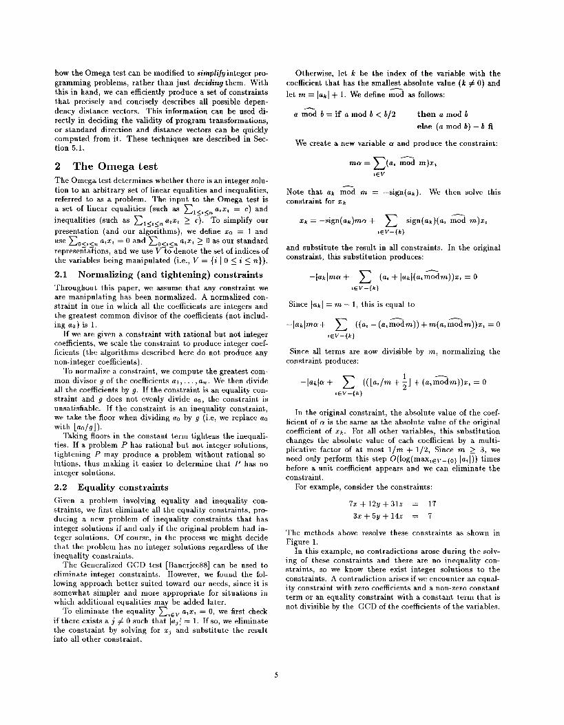
For example, consider the constraints:

7x + 12y + 312 = 17

3z+5rJ+14z = 7

The methods above resolve these constraints as shown in

Figure 1.

In this example, no contradictions arose during the solv-

ing of these constraints and there are no inequality con-

straints, so we know there exist integer solutions to the

constraints. A contradiction arises if we encounter an equal-

ity constraint with zero coefficients and a non-zero constant

term or an equality constraint with a constant term that is

not divisible by the GCD of the coefficients of the variables.

substitution resulting constraints

x=–8cr-4y -z-l –7a–2y+3z=3

–24cr-7y+ llz= 10

y=cr+3p –3a–2/3+z=l

–31cl – 21p + 112 = 10

z=3cr+26+l 2ff+b =-1

18=–20–1 I I

Figure 1: Example of elimination of equatity constraints

2.3 Inequality constraints

The following process is used once all equality constraints

have been eliminated. We first check to see if anv two in-

equality constraints directly contradict one another (e. g.,

the constraints 3X + 5y ~ 2 and 3X + 5y s 0). If we find a

contradiction, we report that the problem has no solutions.

We can deal with equality constraints more efficiently than

inequality constraints. Therefore, if we find a pair of tight

inequalities (such as 6 ~ 3X + 2y and 3X + 2zJ ~ 6), we

replace them with the appropriate equality constraint and

revert to our methods for dealing with equality constraints.

W bile checking for contradictory pairs of constraints, we

also eliminate constraints that are made rednndant by an-

other constraint (e. g., given z + 2y ~ O and x + 2y ~ 5, the

first constraint is redundant).

If the problem involves at most one variable, we report

that it has integer solutions. If the moblem involves more

than one variable, we apply Fourier-Motzkln variable elim-

ination [DE73] in an attempt to prove that there are no

integer solutions. In most cases arising in practice, this

elimination is emxcti it produces a new problem that has

integer solutions if and only if the original problem has in-

teger solutions. If this test cannot disprove the existence of

integer solutions and the elimination is not exact, we ap-

ply an adaptation of the Fourier-Motzkln method we have

devised that, if it reports true, guarantees that an integer

solution exists. This test can confirm integer solutions in

most of the cases that have integer solutions but not exact

eliminations.

If neither of these tests are decisive, we then apply a test

that makes use of the fact that the only integer solutions

that can slip through the crack between the two tests must

have very special forms.

2.3.1 The details

Consider two inequalities ~t=v a,x, ~ O and ~,cv a~x, ~

O, where a~ > 0 > a~. The first of these is a lower bound

on x~ and the second is an upper bound. Resolving these

in terms of x~ produces:

Multiplying through by –aj and ak respectively gives:

This is the key observation of Fourier-Motzkln variable elim-

ination.

We first attempt to disprove the existence of integer so-

lutions to P. We do this by checking if there is an integer

solution to a new problem P’ that contains all inequalities

in P that do not involve z L. and all inequalities moduced

by combining (as shown above) each psi; of upp;r bound

and lower bound on z~. For example, if ~,cv a,z, ~ O is a

lower bound on xk and ~z=v a~x, ~ O is a; upper bound

on Zk in P, the problem P’ contains:

There is a rational solution to P’ if and only if there is

a rational solution to P. This is staudard Fourier- Motzkin

variable elimination [DE73]. More directly related to the

problem at hand, the lack of integer solutions to P’ rules

out the existence of integer solutions to P. Tightening the

constraints of P’ can be very important in verifying that P’

does not have integer solutions.

There is an integer solution for Xk to

if and only if there is a multiple of [a~a~ I between the upper

and lower bounds. Consider the case where the upper and

lower bounds are as far apart as possible, and yet there is

not a multiple of I“k a~ I between them.

Since there doesn’t exist a multiple of Iak a~ I between the

upper and lower bound, there must exist a j such that the

upper bound is less than (j+ l)la~a~ I and the lower bound is

greater than jla~ a~ 1. Since the upper bound is a multiple of

ak it is at most (~ +l)laka~l — la~ I and since the lower bound

is a multiple of a~ it is at least jla~a~ I + “k. Therefore, the

maximum distance between the upper and lower bound is

laka~ I – la~ I – “k. If the distance between the upper and

lower bound is greater than this, a multiple of “k a~ must

exist between them.

Our adaptation of Fourier-Motzkln variable elimination

is to produce a second problem P“, which contains every

inequality in P that does not involve x~ and the result of

combining each pair of upper and lower bounds on Xk in P

to produce a new inequality

If there is an integer solution to P“, we know there is an

integer value of z~ that extends that solution for l’” to be

an integer solution to P.

When the set of integer points described by P’ and P“

are the same, there will be an integer solution to P’ if and

only if there is an integer solution to P. This is referred to

as an ezact eiirninatzors. If all the upper bound coefficients

of z~ are —1. or all the lower bound coefficients of z~ are 1,

the elimination is maranteed to be exact. The elimination

is also guaranteed to be exact if the only constraints having

non-unit coefficients for Xk produce inequalities of the form

aO ~ O (where ao is greater than zero in P“). In these cases,

6

the Omega test takes advantage of the fact that we don’t

have to consider both P’ and P“.

What if P’ has integer solutions but P“ does not have

integer solutions? Then we know that if there is an inte-

ger solution to P, it is tightly nestled between some pair

of upper and lower bounds. Let m be the most negativecoefficient of x k in any inequality. We know that if an in-

teger solution exists, there must exist some lower bound

~,ev a,z, >0 on X, such that

We consider each lower bound ~, ~v a, z, ~ O on z~ in turn.

For ~ in the range O to [(lmakl–lml –ak)/lmlJ, we produce

a new problem Pj containing the constraints of P and the

equality constraint:

akzk = j+ E —a, x,

,cV–{k}

If we find an integer solution to some Pj, we report the

exist ence of integer solutions to original problem.

If we don’t find solutions for any Pj, we change in P the

lower bound just considered to

and check if we can now disprove the existence of integer

solutions to P. If so, we report that there are no integer

solutions to P. Otherwise, we move on to the next lower

bound on Z,$. If we have exhausted the lower bounds on Xk,

we report that no solution exists.

2.3.2 Choosing which variable to eliminate

We try to perform an exact elimination if possible, and

choose the variable that minimizes the number of con-

straints resulting from the combination of upper and lower

bounds. If we are forced to perform non-exact reductions,

we choose a variable with coefficients as close to zero as pos-

sible. We expect that few, if any, inexact eliminations will

arise in the analysis of typical programs.

2.3.3 An Omega test nightmare

To demonstrate (and show the limitations of) the techniques

used, we illustrate the steps performed by the Omega test

on an example designed to force the Omega test to work

very hard for a small problem. Consider the inequalities

There are no exact eliminations we can perform. We

decide to eliminate z since the coefficients of x are (slightly)

smaller. Rearranging the inequalities to be upper and lowerbounds on T give.:

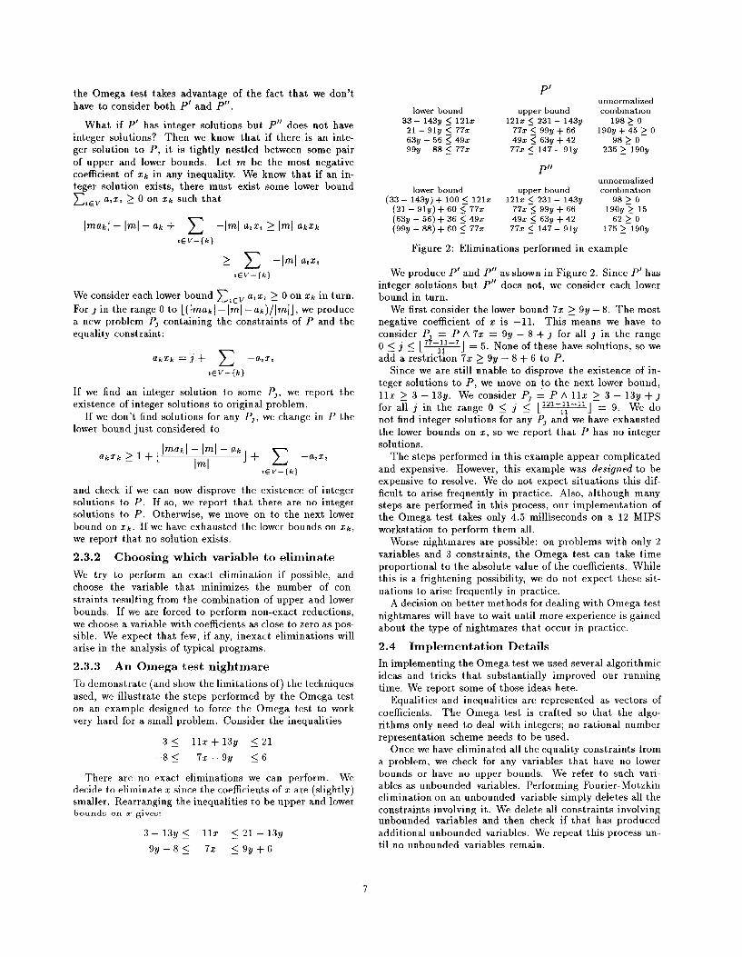
P’unnormalized

lower bound upper bound combination33– 143y < 121C 121z <231 – 143y 1982 (1

21 – 91y < 77X 77X < 99y + 66 190y + 45 ~ o63y – 56< 49c 49z < 63y +42 98~099y – 88< 77X 77X < 147– 91y 235 ~ 190y

p,!

unnormalizedlower bound upper bound comb mat mn

(33- 143y)+ 100< 121z 121x <231 – 143y 98>0(21 – 91y)+ 60< 77x 77X ~ 99y + 66 190y> 15(63y - 56)+36 <490 49c < 63y + 42 62~0(99y - 8S) + 60< 77x 77x < 147– 91y 175 ~ 190y

Figure 2: Eliminations performed in example

We produce P’ and P“ as shown in Figure 2. Since P’ has

integer solutions but P“ does not, we consider each lowerbound in turn.

We first consider the lower bound 7x ~ 9y – 8. The most

negative coefficient of z is —11. This means we have to

consider P = P A 7x = 9y – 8 + j for all J in the range

O S j < [*J = 5. None of these have solutions, so weadd a restriction 7X ~ 9y – 8 + 6 to P.

Since we are still unable to disprove the existence of in-

teger solutions to P, we move on to the next lower bound,

11x ~ 3 – 13y. We consider Pj = PA 11x > 3 – 13y +j

for all j in the range O < j ~ [“’-~~-”] = 9. We do

not find integer solutions for any PJ and we have exhausted

the lower bounds on z, so we report that P has no integer

solutions.

The steps performed in this example appear complicated

and expensive. However, this example was designed to be

expensive to resolve. We do not expect situations this dif-

ficult to arise frequently in practice. Also, although many

steps are performed in this process, our implementation of

the Omega test takes only 4.5 milliseconds on a 12 MIPS

workstation to perform them all.

Worse nightmares are possible: on problems with only 2

variables and 3 constraints, the Omega test can take time

proportional to the absolute value of the coefficients. While

this is a frightening possibility, we do not expect these sit-

uations to arise frequently in practice.

A decision on better methods for dealing with Omega test

nightmares will have to wait until more experience is gained

about the type of nightmares that occur in practice.

2.4 Implement at ion Details

In implementing the Omega test we used several algorithmic

ideas and tricks that substantially improved our running

time. We report some of those ideas here.

Equalities and inequalities are represented as vectors of

coefficients. The Omega test is crafted so that the algo-

rithms only need to deal with integers; no rational number

represent at ion scheme needs to be used.

Once we have eliminated all the equality constraints from

a problem, we check for any variables that have no lower

bounds or have no upper bounds. We refer to such vari-

ables as unbounded variables. Performing Fourier- Motzkin

elimination on an unbounded variable simply deletes all the

constraints involving it. We delete all constraints involving

unbounded variables and then check if that has produced

additional unbounded variables. We repeat this process nn-

til no unbounded variables remain.

7

Next, we normalize all the constraints and assign hash

keys and constraint keys to them. We only do this to con-

straints that have been modified since the last time they

were normalized. The constraint key of a constraint is a

unique tag based on the coefficients of the variables in the

constraint; two constraints have equal constraint keys if and

only if they differ only in their constant term. Keys are

both negative and positive, and the key of a constraint el

is the negation of the key of a constraint ez if and only if

the coefficients of the variables in e] are the negation of the

coefficients of the variables in e2. We refer to this as op-

posing keys and opposing constraints. Constraint keys are

assigned to constraints in constant expected time by record-

ing in a hash table constraint keys previously assigned. We

compute a hash key based on the coefficients of the con-

straint as an index into the hash table (hash keys are not

guaranteed to be unique). Our method for computing hash

keys is designed so that opposing constraints have oppos-

ing hash keys, which makes it easy to assign them opposing

constraint keys. As constraints are normalized, we enter

them into a table based on their constraint key. This allows

us to check for redundant, contradictory or tight constraint

pairs in constant time per constraint.

In the process of normalizing constraints, we check to see

if any constraints involve more than one variable. After

normalization, if we found no multi-variable constraints, we

know the system must have solutions, and we return imme-

diately.

Next, we examine the variables to decide which variable

to eliminate. If we can perform an exact elimination, we

perform the elimination in place (adding and deleting con-

straints from the current problem). Otherwise, we copy the

constraints not involved in the elimination into two new

problem data structures (for P’ and P“) and then add the

constraints produced by Fourier-Motzkin elimination. Since

P’ and P“ differ only in their constant term, we can share

much of the work in creating these problems.

3 Nonlinear subscripts

Integer programming dependence analysis methods allows

us to properly handle symbolic constants [LT88, HP90] and

some types min and max functions in loop bounds [WT90]

and and conditional assignments [LC90].

For example, even if we had no information about the

value of n, we would like to be able to decide that there are

no flow dependence in the following program:

fori=l tondo

a[i+nl = a[i]

As previous authors have suggested, we can handle loop-

invariant symbolic constants by adding them as additional

variablen to the integer programming problem. For exam-

ple, the above problem would generate the following integer

programming program (involving the variables z, t’ and n):

1<2,2’<n

2+n=i’

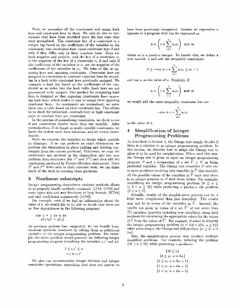
We also can accommodate integer division and integer

remainder operations, something that does not appear to

have been previously recognized. Assume an expression e

appears in a program that can be expressed ss

()‘= ‘+5”’ ‘ivm,=1

where m is a positive integer. To handle this, we define a

new variable a and add the inequality constraints

,=1

and use a as the value of e. Similarly, if

()‘= C+b’ ‘odm*=1

we would add the same inequality constraint but use

n

—ma+c+~a, x,

,=1

as the value of e.

4 Simplification of Integer

Programming Problems

As described in Section 2, the Omega test simply deczdes if

there is a solution to an integer programming problem. In

this section, we describe how to adapt the Omega test to

allow it to be used for sirnplzjication. When used this way,

the Omega test is given as input an integer programming

program P and a designation of a set V c V as being

protected variables. The Omega test simpli@ P into one

or more problems involving only variables in V that describe

all the possible values of the variables in V such that there

is an integer solution to P with those values. For example,

simplifying the integer programming problem {O ~ a ~

5; 6 < a < 5b} while protecting a produces the problem

{2~a~5}.

Actually, results of the simplification process can be a

little more complicated than just described. The results

“. Instead, themay not be in terms of the variables in V

results are given in terms of a set ~’ of not more than

Ifil variables (possibly including new variables), along with

methods for calculating the appropriate values for the values

of V from the values of ~’. For example, if asked to simplify

the integer programming problem {a = 10tJ + 25c; a ~ 13}

while protecting a, the Omega test will produce {a z 3; a =

5ff}.

Also, the simplification process may produce multiple

simplified problems. For example, reducing the problem

{5b ~ a ~ 6b} while protecting a produces:

{20 ~ a}

{O~a; a=6rv}

{l<a; a=6a-1}

{2~a; a=6a-2}

{3~a; a=6rr-3}

8

4.1 Complicated results from simplification

All the Omega test does is s~mplify a proble~ to a sys-

tem of constraints involving IV I variables. If IVI is greater

than one, the simplified problem may involve redundant

constraints, although it does not contain any contradictory

ones (nor any redundant pairs).

4.2 Changes to the Omega test

Three of the changes required are simple, the other is not

as simple. The quick changes are:

● If the current problem P involves only protected vari-

ables, check if there are integer solutions of P and ifso, report P as one simplification.

● When performing an inexact Fourier-Motzkin elimina-

tion, simplify P“ and all the Pj for all lower bounds(not stopping when an integer solution is first veri-

fied). This could be expensive if simplifying a system

involves many inexact eliminations. We do not believe

this will occur in practice for the problems arising from

dependency analysis.

● We never perform Fourier-Motzkin variable elimina-

tion on a protected variable. This could require us to

perform a non-exact elimination in a situation where

we could have performed an exact elimination if we

were not protecting certain variables.

The not so simple change involves equalities. Given an

equality constraint ~,c” a,z, = O, let g be the gcd of the

coefficients of the non-protected variables. (we assume (as

always) that the constraint is normalized).

● If g = O, the constraint involves only protected vari-

ables. We use our standard methods to eliminate the

constraint. This will result in the elimination of a pro-

tected variable. All substitutions performed in this

process are recorded in a substitution log. These sub-

stitutions involve only protected variables.

● If g = 1, we use our standard techniques (Section 2.2)

to find a substitution involving only unprotected vari-

ables that simplifies or eliminates the constraint.

● If g >1, we create a new protected variable a, add the

constraint:

x(

.ga = a, mod m)z,

te v

Eliminating this new constraint will transform the orig-

inal constraint so that the gcd of the non-protected

variables is 1 (after normalization).

When we report a simplification, we also report all the

substitutions involving protected variables made while solv-

ing the current problem.

4.3 Simplification with wildcards

As a modification of the approach described above, we couldrefuse to perform inexact reductions while performing sim-

plification. The advantage of this is that we only report one

simplified problem as our result. The disadvantage is that

the simplified problem has additional variables (that should

be treated as wildcards)

In the applications we have found for simplification, we

have found simplification with wildcards to be more useful

than producing multiple results.

5 Using simplification

This simplification technique can be used for several pur-

poses. We describe some that have occurred to us.

5.1 Dependence direction and distance

vectors

One problem with some dependence analysis methods is

that they are only ‘yes/no” decision methods. In com-

pilers and other program structuring tools, we need to

know the data dependence direction vector [W0182] and

data dependence dist ante vector [K MC72, Mur71] describ-

ing the relation between the iterations in which the conflict-

ing reads/writes occur. One way to determine dependence

direction vectors is to make 3L calls to the decision pro-

cedure (where L is the number of loops surrounding both

references). In order to be competitive, a dependence anal-

ysis method must be able to short-cut this enumeration (for

example, see [BC86, GKT91]).

In our method, we take the integer programming prob-

lem for determining if any dependence exists between two

references. and introduce a new variable for the der)endence

distance in each shared loop (along with the ap&opriate

equality constraints to define the value of the variable). We

then simplify the problem down to the dependence distance

variables. The simplified system may be a better way to

describe dependence conditions than dependence directions

and dist antes; it accurately describes more information than

is typically contained in dependence direction vectors (such

as when a dependence dist ante is always greater than 5).

Alternatively, we can use the simplified set of constraints

to determine efficiently the dependence direction and dis-

t ante vectors. We scan the dependence, and infer as much

information as possible from constraints involving a sin-

gle dependence distance variable. Any dependence distance

variable that is uncoupled or who’s sign is completely deter-

mined by uncoupled constraints is unprotected. If coupled

variables were unprotected, we simplify the problem and

repeat this process. Otherwise, we choose one protected

variable and generate the subproblems for two or three pos-

sible signs for the variable (negative, zero or positive), and

recursively explore those.

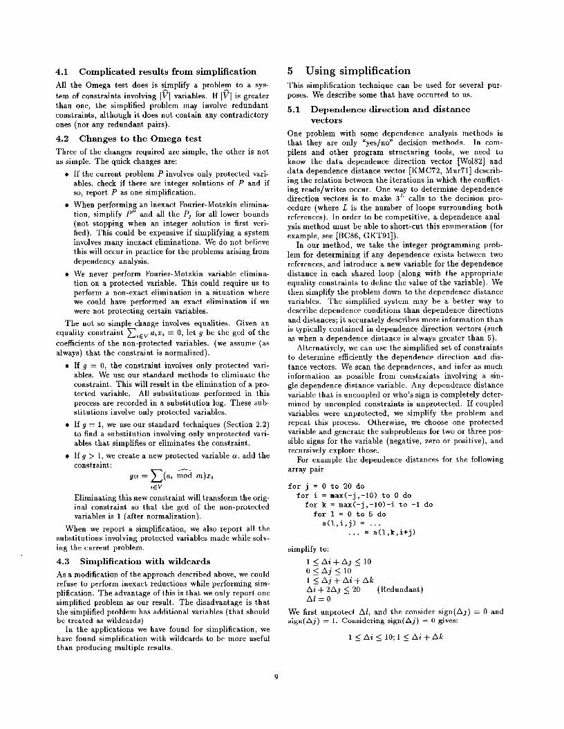
For example the dependence dist antes for the following

array pair

forj=Oto20do

for i = max(-j ,-10) to O do

for k = max(-j, -10)-i to -1 do

forl=Oto5do

a(l, i,j) = . . .

. . . = a(l, k,i+j)

simplify to:

l< Ai+AI <10

o< Aj <10

l< Aj+Az+Ak

Ai + 2A] <20 (Redundant)

Al=o

We first unprotect Al, and the consider sign(Aj) = O and

sign(Aj”) = 1. Considering sign(Aj) = O gives:

l< Az<lO; l< AZ+Ak

9

We would then unprotect Ai (since we know sign(Ai) = 1)

and simplify the problem, obtaining —9 s Ak, or a direction

vector of (=, <, *, =).

Returning to consideration of sign(Aj) = 1 produces:

–95Ais9

–9 s Ak

–9<A2+Ak

–18 ~ Ai+2Ak (Redundant)

Recursively analyzing the possibilities for the sigu of Ai

produces direction vectors of (<,>,*, =), (<,=,*,=) and

(<, <,*, =). This example is the most difficult example seen

in our testing, requiring 1890 psecs to analyze.

5.2 Summarizing Array References

In interprocedural analysis, we need to characterize the por-

tions of an array that may be affected by a procedure call

[Tri85, BK89, HK90, IJT91]. We can use the Omega test

to obtain an accurate summary of the locations of an array

that might be affected by a single assignment statement.

We do this by setting up an integer programming problem

involving variables for each array index and all loop vari-

ables and symbolic constants, and adding appropriate con-

straints for the loop bounds, subscript expressions, and so

on. Simplifying this problem, while protecting the variables

for the array indices and the symbolic constants, gives an

accurate summary of the locations of the array affected by

the assignment statement. The summary is not limited to

convex polyhedron. The simplified problem will have solu-

tions only for those locations’ that can actually be changed.

Details such as strides are accurately represented.

The Omega test can easily be used to determine when

two regions intersect. With more work, the Omega test

can be used to check if one region is a subset of another.

It is unclear how to use the Omega test to merge affected

regions; however, the Omega test could be used to convert

exact affected regions into approximate affect regions (such

as described by [BK89, HK90]) and then those regions could

be merged.

5.3 Determining Loop Bounds

The Omega test can be used to determine appropriate loop

bounds when interchanging non-rectangular loops. Ths use

of integer programming to perform this is described by

[A191].

6 Performance

We have implemented the Omega test in Wolfe’s tiny tool

[WO191]. We handle min and max expressions in loop bounds

and symbolic constants, and compute exact sets of direc-

tion vectors (aa opposed to the compressed direction vectors

normally generated by tiny). We applied this tool to the

programs 1, 3, 4, 5 and 7 of the NASA NAS benchmark

suite and to all the tiny source files distributed with tiny,

(which include Cholesky decomposition, LU decomposition,

several versions of wavefront algorithms, and several more

contrived examples), as well as several of our own test pro-

grams. Programs 2 and 6 of the NAS benchmark make

extensive use of index arrays. Since we do not provide spe-

cial treatment for index arrays, we decided that it would be

misleading to include them. The analysis of array pairs that

have different constant subscripts (e.g., a (4) and a(5)) are

2000 I I I o t

t% A

1000

500anrdysis

time

(psecs)

250

I

100

“A.”-” -

t /’ “-’‘1 complex W_~~,I I

50 75 100 150

copy time (~sec)

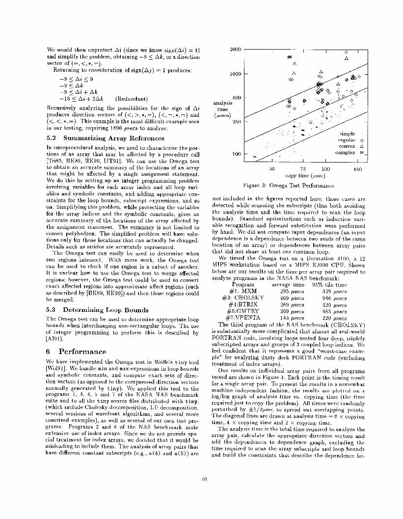
Figure 3: Omega Test Performance

not included in the figures reported here; those cases are

detected while scanning the subscripts (thus both avoiding

the analysis time and the time required to scan the loop

bounds). Standard optimizations such as induction vari-

able recognition and forward substitution were performed

by hand. We did not compute input dependence (an input

dependence is a dependence between two reads of the same

location of an array) or dependence between array pairs

that did not share at least one common loop.

We timed the Omega test on a Decstation 3100, a 12

MIPS workstation based on a MIPS R2000 CPU. Shown

below are our results on the time per array pair required to

analyze programs in the NASA NAS benchmark:

Program average time 95%tile time

#1: MXM 295 psecs 329 psecs

#3: CHOLSKY 469 psecs 946 ~secs

#4: BTRIx 269 psecs 420 psecs

#5: GMTRY 209 psecs 485 psecs

#7:vPENTA 143 ~secs 220 ~secs

The third program of the NAS benchmark (CHOLSKY)

is substantially more complicated that almost all real-world

FORTRAN code, involving loops nested four deep, triplely

subscripted arrays and groups of 3 conpled loop indices. We

feel confident that it represents a good “worst-case exam-

ple” for analyzing dusty deck FORTRAN code (excluding

treatment of index arrays).

Our results on individual array pairs from all programs

tested are shown in Figure 3. Each point is the timing result

for a single array pair. To present the results in a somewhat

machine independent fashion, the resnlts are plotted on a

log/log graph of analysis time vs. copying time (the time

required just to copy the problem). All times were randomly

perturbed by +1/2psec to spread out overlapping points.

The diagonal lines are drawn at analysis time = 8 x copying

time, 4 x copying time and 2 x copying time.

The analysis time is the total time required to analyze the

array pair, calculate the appropriate direction vectors and

add the dependence to dependence graph, excluding the

time required to scan the array subscripts and loop bounds

and build the constraints that describe the dependence be-

10

tween the array pairs 7 Polynomial time boundsAcross a range of test programs, we found the follow-

ing break-down for how time was spent by the Omega test:

about 1/2 the time was spent dealing wit h inequality con-

straints, about 1/4 of the time was spent on dealing withequality constraints, and I/4 of the time was spent exam-

ining simplified constraints to construct direction vectors.

None of our test cases required inexact Fourier-Motzkinvariable elimination.

To analyze our results, the set of constraints describ-

ing the dependence distances for each array pair were ana-

lyzed to remove any redundant constraints (this is not cost-

effective normally). Based on the simplified constraints,

each array pair was classified as follows:

simple Any case that does not involve coupled dependence

dist antes.

regular A case where dependence dist antes are coupled,

but afl inequality constraints have unit coefficients (for

example, {Ai > O;Ai + Aj > O}).

convex A case where the inequality constraints define a

convex region but at least one constraint has a non-unit

coefficient (for example, {O ~ AJ ~ 10; O ~ Ai + Aj <

10; Ai + 2Aj < 10} – the last constraint makes th~

non-regular).

complex A csse where the inequality constraints define a

non-convex region. We only encounted two such cases,

one shown below and another one identical except that

the lower bound of the i loop is 2.

fori=ito lOdo

forj=Oto4do

a(i-j) = a(j)

endf or

end for

The flow/anti dependence distances for the example

above are all the distances that satisfy { –4 < Aj <

4; –7 ~ AZ – Aj, Az + Aj < 10; Ai < 9} except for

{Ai= 9;Aj =0}.

Maydan, Hennessy and Lam [MHL91] use memorization

to obtain better performance. Memorization could be added

to the Omega test. However, the cost of computing a hash

key and verifying a cache hit would be about 2-4 times the

copying cost for a problem, and therefore adding caching to

the Omega test would not produce significant savings for

typical, simple cases and may produce little or no overall

speed improvement.

We found that the cost of scanning array subscripts and

loop bounds to build a dependence problem was typically

2-4 times the copying cost for the problem. Thus, for many

array pairs the cost of building the dependence problem was

nearly as large or even larger than the time spent analyz-

ing the resulting problem. We have not spent much effort

trying to improve the performance of the code that builds

dependence problems. However, it is difficult to imagine

building a dependence problem in much less than twice the

time required to copy the problem. This suggests that for

the majority of array pairs, using a dependence analysis al-

gorithm significantly faster than the Ome~a test would not

lead to significant overall speed improvements.

We first describe some generaf time bounds on parts of the

Omega test, and then describe polynomial time bounds for

cases where other polynomial time algorithms are accurate.

In this section, we use m to denote the number of constraints

and n to denote the denote the number of variables.

The time taken by the methods in Section 2.2 to eliminate

one equality constraint is O(mn log ICI) worst-case time,

where C is coefficient with the largest absolute value in the

constraint. This cost arises from the fact that we might

have to apply the perform log [Cl substitutions before we

can eliminate the constraint, and performing a substitution

takes O(nm) time.

Eliminating unbound variables takes O(rnrLp) worst-case

time, where p is the number of passes required to eliminate

all the variables that become unbound. At least one variable

is eliminated in each pass except the last.

Normalizing the constraints and checking for directly

contradictory or redundant constraints requires O(mn) ex-

pected time (the time bound is only expected, not worst-

case, because hashing is used).

Producing the subproblems resulting from Fourier-

Motzkin variable elimination takes time proportional to the

size of the subproblems produced.

7.1 Special cases

During normalization, the Omega test checks to see if any

variables are involved in constraints with other variables.

If not (and checking for contradictory constraint pairs has

not moduced a contradiction), we know the problem has

solu~ions and do not need to perform any additional com-

putation. This applies iff the ‘Single Variable Per Con-

straint” (SVPC) test [MHL91] can be applied, which was

found [MHL91] to be applicable in 1/3 of the unique cases

found in the Perfect Club Benchmark (a higher percentage

if duplicate cases were considered separately).

The “Acyclic Test” [MHL91] can be applied in exactly

those cases that the Omega test can resolve just by elimi-

nating unbound variables and performing exact eliminations

that do not increase the number of constraints, a process

that takes O(mn2 ) worst-case time. They found [M HL91]

that this test could be applied in over 1/4 of the unique

cases encountered.

The “Loop Residue” algorithm [Sho81] can be applied in

iust those cases where each constraint is of the form x, >

zj+c, x,>c, ore> x,. In a set of constraints with

this property, Fourier-Motzkin variable elimination is exact

and preserves this property. On n variables, there can be

at most n2 + n constraints of this form after eliminating

redudant pairs. Thus, the Omega test will take O(n3 ) time

to resolve a set of constraints that can be solved by the Loop

Residue algorithm. Maydan, Hennessy and Lam [MHL91]

found that the Loop Residue algorithm could be applied

in 1/4 of the unique cases encounted in their study of the

Perfect Club benchmark.

Maydan, Hennessy and Lam found that 91% of the cases

they encountered could be determined by constant tests and

Banerjee’s Generalized GCD tests. Of the remaining 9?Z0 of

the cases, they found that their SVPC, Acyclic or Loop

Residue tests could be appIied in 86% of the unique cases.

The Delta test [GKT91] works by searching for depen-

11

dence distances that can be easily determined, and then

propagating that information with the intent of making it

possible to easily determine other dependence distances pre-

cisely. In the cases where their algorithm can determine

a dependence distance without the use of MIV tests, the

Omega test also will determine it efficiently (and in polyno-

mial time) by a combination of solving equality constraints,

tightening inequality constraints and converting tight in-

equality constraints into equality constraints. Since the

Omega test treats the dependence analysis problem as a sin-

gle integer programming problem, it automatically achieves

the propagation effects of the Delta test. Therefore, any de-

pendence analysis problem that can be solved by the Delta

test without resorting to exponential algorithms or approx-

imate methods (i.e., resorting to what they refer to as MIV

tests) can be solved in polynomial time by the Omega test.

In their study of the RiCEPS, Perfect, SPEC benchmarks

and LINPACK and EISPACK, they found that 97% percent

of the cases could be solved without requiring the use of

MIV tests.

Since the Omega test can solve effectively and in (effec-

tive) polynomial time any problem that be solved by any

combination of the Single Variable Per Constraint test, the

Acyclic test, the Loop Residue test and the Delta test, we

expect that it should be able to solve more problems exactly

and efficiently than any one of them alone.

8 Related work on Exact Dependence

Analysis

The Constraint-Matrix test [Wa188] makes use of the sim-

plex algorithm modified for integer programming. The

Constraint-Matrix test can fail to terminate and not clear

how efficiently it works in practice.

Lu and Chen describe [LC90] an integer programming

algorithm for dependence analysis. However, their method

appears prohibitively expensive for use in a production com-

piler.

Triolet [Tri85] used Fourier-Motzkin techniques for rep-

resenting affected array regions in interprocedural analysis.

Triolet found Fourier-Motzkln techniques to be expensive

(22 to 28 times longer than using simpler methods for rep-

resenting affected array regions).

SeveraJ implementations of Fourier-Motzkin variable

elimination have been described for use in dependence and-

ysis. The Power test described by Wolfe and Tseng [WT90]

combines the Banerjee’s Generalized GCD test, constraint

tightening, and Fourier- Motzkin variable elimination. They

take no special action when performing an inexact elimina-

tion except to flag the result as possibly being conservative.

Fourier-Motzkln elimination is used by by Maydan, Hen-

nessy and Lam [M HL91] if none of the other methods they

use They use back substitution to determine a sample so-

lution. If the sample solution is not integral, they suggest

the use of branch and bound methods to verify or disprove

the existence of integer solutions (they have not found the

need to implement this thus far). Both Wolfe and Tseng

[WT90] and Maydan, Hennessy and Lam [MHL91] suggest

that due to the expense of Fourier-Motzkin variable elim-

ination, simpler tests should be used instead in situations

where they are known to be accurate.

Ancourt and Irigoin [A191] describe the use of Fourier-

Motzkin variable eliminate to simplify, or project, an inte-

ger programming problem (the concept described in Section

4) so as to determine loop bounds for iterating over an iter-

ation space described by a set of linear inequalities. Their

work has significant overlaps with ours. The key differences

between our work and their work is as follows:

They do not describe any special techniques for han-

dling equality constraints, although they could easily

use Banerjee’s Generalized GCD test.

They do not describe any performance data on their

algorithm.

Thev handle inexact elimination bv introducing

pseudo-linear constraints into the problem. There are

useful useful for producing loops that iterate over a

space described by a set of linear inequalities, but it is

unclear how to use them when attempting to verify or

disprove the existence of integer solutions.

When performing an inexact elimination, they produce ~

problem equaJ to our P’. They also consider a problem P

that is similar to our P“ except they use force the difference

between the upper and lower bounds to be at least la~a~ I –

la~], as opposed to laka~l – Iajl – ak + 1 for P“. Since ~ is

more conservative than P“, using P“ gives better results.

They do not actually generate ~ a: a separate problem.

Rather, they check the constraints in P that differs from the

constraints of P’sand see if those constraints are redundant

with respect to P. If so, then P’ is an exact reduction. In

other words, they check if P’ ~ P. If so, since P ~ P’, we

known that P’ = ~ and t~at the elimination is exact,.

If some constraint in P is not redundant with respect

to the constraints of P’, then they add p.sezdo-linear con-

straints to P’ so that P’ has integer solutions iff P has

integer solutions. These pseudo-linear constraints appear

useful and appropriate for determining loop bounds. How-

ever, they are difficult to use for determining the existence

of integer solutions.

A recent report [IJT91] on the PIPS project mentions

that Fourier-Motzkin variable elimination is used to ana-

lyze dependence (based on the work described in [A191]).

The methods used are not fully described, but the basic

framework appears similar to that described in Section 5.1,

It is not clear how the pseudo-linear constraints of [A191]

are handled. They point out that in many simply cases,

Fourier-Motzkin variable elimination is fast and efficient.

They state that using integer programming techniques for

dependence analysis inccurs a very high cost (that is ac-

ceptable sinces PIPS is not a production system). They

also state that in their implementation dependence testing

does not take a noticeable amount of time compared with

the whole parallelization process.

9 Source code availability

A C language implementation of the Omega test is freely

available for anonymous f tp from f tp. cs. umd. edu in di-

rectory pub/omega.

12

10 Conclusions

Conservative dependence analysis methods may be effica-

cious for the demands of vectorizing compilers. Trans-

forming programs so as to make efficient use of massively

parallel SIMD computers is a much more demanding task.

Also, programs that have undergone transformations such

as look skewing and loop interchange present analysis prob-

lems substantially more difficult than encountered in typical

dusty-deck FORTRAN.

Our studies have convinced us that the Omega test is a

fast and practical method for performing data dependence

analysis that is not only adequate for problems encountered

in vectorizing FORTRAN code, but also for the demands of

more sophisticated program transformation tools.

Performing simplification of integer programming prob-

lems is an exciting concept. We have discussed how it can be

used to determine efficiently information about dependence

direction and distance vectors, as well for several other uses.

It much easier to describe and build program analysis and

transformation tools. For example, it can be used for deter-

mining loop bounds after loop interchange [A191], and we

have made extensive use of it in work that considers loop

transformations in a uniform manner [Pug91].

11 Acknowledgements

Thanks to everyone who gave me feedback on this work,

especially Michael Wolfe and the anonymous referee who

provided detailed comments.

References

[A191]

[AK87]

[AH83]

[Ban88]

[BC86]

[BK89]

[DE73]

[GKT91]

[HK90]

Corirme Ancourt and Pranqois Irigoin. Scanning poly-

hedra with do loops. In PPOPP ’91, 1991.

J. R. Allen and K. Kennedy. Automatic translation ofFortran programs to vector form. ACM Transactions

on Programming Languages and Systems, 9(4):491–

542, October 1987.

J. R. Allen. Dependence Analysis jor Subscripted

Variables and Its Application to Program Transjor-matio ns. PhD thesis, Rice University, April 1983.

U. Banerjee. Dependence Analysts jor Supercomput-ing. Kluwer Academic Publishers, Boston, MA, 1988.

M. Burke and R. Cytron. InterProcedural dependenceanalysis and parallelization. In em Proceedings of the

SIGPLAN ’86 Symposium on Compiler Construction,

Palo Alto, CA, Jtiy 1986.

V. Balasundaram and K. Kennedy. A technique for

summarizing data access and its use in parallelism en-hancing transformations. In SIGPLA N Conference on

Pvogmmming Language Design and Implementation,’89, June 1989.

G .B. Dantzig rmd B.C. Eaves. Fourier- Motzkin elirn-nation and its dual. Journal of Combinator-ial Theory

(A), 14:288-297,1973.

G. Goff, Kenn Kennedy, and Chau- Wen Tseng. Prac-

tical dependence testing. In ACM SIGPLAN’91 Con-je,ence on Programming Language Design and Imple-

mentation, 1991.

Paul Havlak and Ken Kennedy. Experience with in-terprocedural analysis of array side effects. In Super-computing ’90, 1990.

[HP90]

[IJT91]

[KMC72]

[LC90]

[LT88]

[LY90]

[LYZ89]

[MHL91]

[Mur71]

[Pug91]

[Sh081]

[Tri85]

[wa188]

[WC1182]

[W0189]

[wcd91]

[WT90]

M. Haghighat and C. Polychronopoulos. Symbolic de-pendence analysis for high performance parallelizing

compilers. In Proceedings oj the Third Workshop on

Languages and Compilers for Parallel Computing, Au-

gust 1990.

PranSois I.tigoin, Pierre Jouvelot, and R6mi Trio-

Iet. Semanticaf interprocedural parallelizatiorc Anoverview of the pips project. In ICS ’91, 1991.

D. Ku&, Y. Muraoka, and S. Chen. On the number of

operations simultaneously executable in FORTRAN-like programs and their resulting speedup. IEEE

Transactions on Computers, 1972.

L. Lu and M. Chen. Subdomain dependence test formassive parallelism. In Proceedings o.f Supercomputing

‘9o, New York, NY, November 1990.

A. Lichnewsky and F. Thomasset. Introducing sym-bolic problem solving techniques in the dependence

testing phases of a vectorizer. In Proceedings o-f theSecond International Conference on Supercomputing,

St. Male, France, July 1988.

Z. Li and P. Yew. Some results on exact data de-pendence anrdysis. In D. Gelernter, A. Nicolau, and

D. Padua, editors, Languages and Compders for Par-allel Computing. The MIT Press, 1990.

Z. Li, P. Yew, and C. Zhu. Data dependence analysison multi-dimensional array references. In Proceedings

oj the 1989 ACM International Conference on Super-computing, June 1989.

D. E. Maydan, J. L. Hennessy, and M. S. Lam. Ef-

ficient and exact data dependence analysis. In A Ckf

SIGPLAN’91 Conference on PTogTamming LanguageDesign and Implementation, 1991.

Y. Muraoka. Parallelism EzposuTe and Ezplottatton

in Programs. PhD thesis, Dept. of Computer Science,

University of Illinois at Urbana-Champaign, February1971.

William Pugh. Uniform methods for loop optimizat-

ion. In 1991 International Conjer-ence on Supercom-puting, Cologne, Germany, June 1991.

R. Shostak. Deciding linear inequalities by computing

loop residues. Journal oj the A CM, 28(4):769--779,October 1981.

R. Triolet. InterProcedural analysis for program re-structuring with Parafrase. CSRD Rpt. 538, Dept.

of Computer Science, University of Illinois at Urbana-Champaign, December 1985.

D. Wallace. Dependence of multi-dimensional array

references. In Proceedings oj the Second IntemtationalConference on Supercomputing, St. Male, France, July1988.

M. J. Wolfe. Optimizing Supercompilers jor Super-

comput em. PhD thesis, Dept. of Computer Science,University of Illinois at Urbana-Champaign, October1982.

Michael Wolfe. Optimtmng Supercompilers jor Super-computers. Pitman Publishing, London, 1989.

Michael Wolfe. The tiny loop restructuring research

tool. In Proc of 1991 International Conference on

Parallel P~ocess8ng, 1991.

Michael Wolfe and Chau-Wen Tseng. The power testfor data dependence. Te&lcal Report CS/E 90-015,Oregon Graduate Institute, August 1990.

13