THE OfflO STATE UNIVERSITY

•

O.S.Ü. R.F. 8177-1

RESEARCH FOUNDATION 1314 KINNEAR ROAD COLUMBUS, OHIO 43212

STRESSES, DEFORMATIONS AND PROGRESSIVE FAILURE OF NON-HOMOGENEOUS FISSURED ROCK

Semi-annual Technical Report« August SO, 1971

U.S. Bureau of Mines, Contract No. HO210017

Sponsored by Advanced Research Projects Agency ARPA Order No. 1679, Amend. 2 Program Code IFIO

The views and conclusions contained in this document are those of the authors and should not be interpreted as necessarily representing the official policies, either expressed or implied, of the Advanced Research Projects Agency or the U.S. Government.

Reproduced by

NATIONAL TECHNICAL INFORMATION SERVICE

Sprlngliold, Vl. 22151

ns

BEST AVAILABLE COPY

,"~

-'

UNCLASSIFIED

fei unu n.

3?00.8 (AU 1 to Eae3 l) Mar 7, C6

DOCUMENT CONTROL DATA ■ fi .. D

t OF. lOIN A I U, ,, AC

The Ohio State University Research Foundation

-a. (. t r on i v c: uhi i i c i A •.

Unclassified

i C;<I»«I»C

11 I (CAM

3 HLMOKT TITLI

STRESSES, DEFORMATIONS AND PROGRESSIVE FAILURE OF NON- HOMOGENEOUS FISSURED ROCK

4 DtSCHiMllVLNOTts fTVpt o/ T' port flftd /nc/usive dale»)

Semiannual Technical Report - February 1, 1971 - July 31, 1971 V AU THORIS) f/-*if vf rdJTie, r:id !U- inHiel. Iislncj.c)

R. S. Sandhu, T. H. Wu and J. R. Hooper

6. REPORT DATE

August 30, 1971 9». CONTRACT ON GHANT NO.

HO210017 b. PRO.' CC T NO

RF 3177 Al

7«. TOTAL NO OPPAOES

100 7h. NO, OF RKF5

44 items 9a. ORIOIK A 1 OR'S REPORT NUMDERIS)

None

S^. OTHER r-t.POT'.T t.om (Afiy other ir this report)

ibota Um! may be Itittigrioti

None 10. DISTRIBUTION STATEMENT

Distribution of this document is unlimited.

II. SUMPUrMLNTART NTTES II?. SPONSORING Mit.1' AR ¥ ACIIVITT

Advanced Research Projects Agency Washington, D.C. 20301

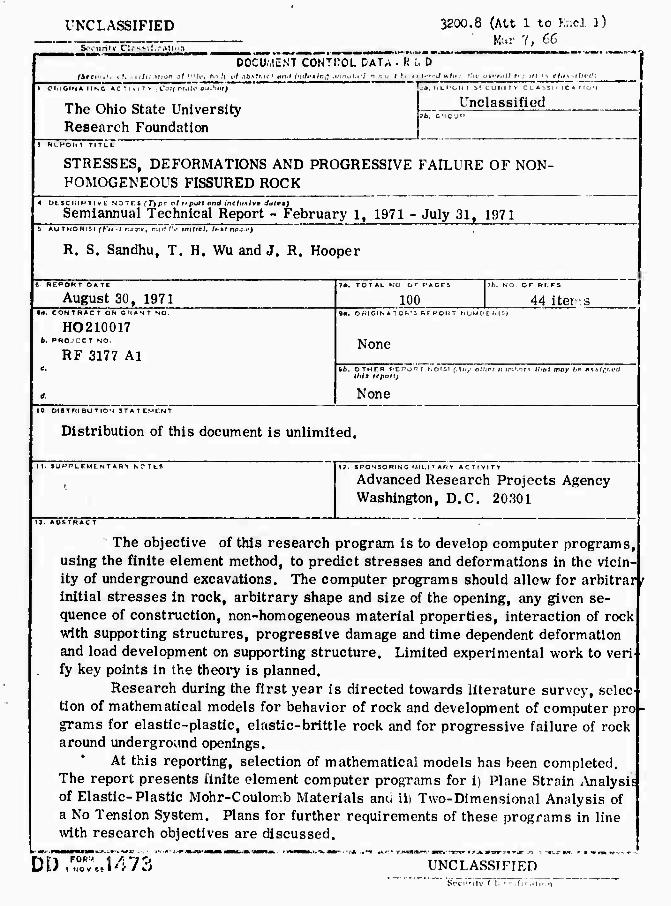
13. ABSTRAC T

The objective of this research program is to develop computer programs, using the finite element method, to predict stresses and deformations in the vicin ity of underground excavations. The computer programs should allow for arbiträr^ initial stresses in rock, arbitrary shape and size of the opening, any given se- quence of construction, non-homogeneous material properties, interaction of rock with supporting structures, progressive damage and time dependent deformation and load development on supporting structure. Limited experimental work to veri' fy key points in the theory is planned.

Research during the first year is directed towards literature survey, selec- tion of mathematical models for behavior of rock and development of computer pro grams for elastic-plastic, elastic-brittle rock and for progressive failure of rock around underground openings.

At this reporting, selection of mathematical models has been completed. The report presents finite element computer programs for i) Plane Strain Analysi of Elastic-Plastic Mohr-Coulomb Materials anu iii Two-Dimensional Analysis of a No Tension System. Plans for further requirements of these programs in line with research objectives are discussed.

Dt) I NO¥t»14 / J UNCLASSIFIED 8eci"ily Cli ■ ■ ifi'vn

INCI ASSIFILD 55C0.3 (Att 1 to ■aol l)

computation

deformation

elasticity

excavation

failure

finite element method

foundations

mining

plasticity

progressive failure

research

rock mechanics

stresses

tunnels

underground excavation

LtSM *

1.1: ■ t rt r «o i r: ft '

^CLASSIFIED Si r'Mity CUiSsifli ition

SEMIANNUAL TECHNICAL REPORT

FEBRUARY 1, 1971 - JULY 31, 1971

AR PA Order Number: 1579, A mem I 2

Program Code Number: 1F10

Name of Contractor:

The Ohio State University Research Foundation

Contract Number: HO210017

Principal InvestlKators: R. S. Sandhu T. H. Wu J. R. Hooper

Telephone Number: (614) 422-7531

Project Scientist or Engineer:

R. S. Sandhu

Telephone Number: (014)422-7531

Effective Date of Contract:

February 1, 1971

Contract Expiration Date:

January 31, 1972

Amount of Contract:

$46,113

Short Title of Work:

Stresses, Deformations and Progressive Failure of Non- Homogeneous Fissured Kock

This research was supported by the Advanced Research Projects Agency of the Department of Defense and was monitored by Bureau of Mines under Contract Number HO210017.

Distribution of this document is unlimited.

I I I I 1

IivhuUil Rtport Suinmnry

Ilu- ohUill\f '»f thl?» rt'j*f uvh pr«»ur.im Is •«» cU'velop compulcr prournntM,

using the ftntte »Unu-nt metlvHl, to prcHliot siroHxcn an«! «Iffttrmailon« In Ihf vlcin-

liy .»i imdergr «ml f\iM\.Uli»ns. Ilu compuliT itnturam» will havi- tlu- fapaltllltv

to all m for arl>ltiMr> InlU.il siivMSfs in nK'k, arbitrary shape« ami «l/t* of thi-

opmlng, am given Mquvnctof eonstnictiDn, niinhoinu^fni'ttus maiciial proprrth^,

IntfiMiilon •»! r«u-k with Huppnrtinu stnuiun-s, pmurrsslvi« ilamano, ami HUM

dependent cMormatlon ;in«l li»a<l dtveloprowl '»n supiMtrdnK structure. I.imitctl

i\|Hiinu'ni.il work t«» \»i'll\ kiy imlnts In thr ilu*ory Is planned.

lUseareh dulag the first year Is directed towards survi-y of literaturi'

on thf subifci, selection of mathematical models for mechanieal U-havlor of nn-k,

an«! «lovi'Iopment of computi-r pronrams for clastic-plastic Mohr-Coulond» materials,

f<»r hrlttle nnk follovinn Griffith's the«)ry, and for progressive dtformation and

fracture of rock around umlcrnrouml openinKS under stress changes associated with

excavation.

At this reporting, si'Iectlon of mathematical models for elastic-plastic Mohr-

Coutomb materials and for clastic-brittle materials failing accordin« to Cirifflth

theory has been completed. Chaptc r I of the report describes the theoretical con-

sider itions leadin« lo the mr, Icl selected. The stress-strain relations for incre-

mental or rate type theory of plasticity arc «enei ally based on the normality ride

:ind convexity and regularity of the yield surface in I 'stress-space'. Ullflg these

I 1

i

1 I I

rmu'rpls, v;iiious ln\i>lu:i!ors h;i\i' proposed confliCttal (.onstitutivt' equations.

In iiUs rcpiTi thr i-hsth'-plastk- i>i'h;i\i<>r oi matcriali li;is been re-examined as

i m ithi'malical iiem-rali/ation oi »hsi-m ations on a ont'-dinu-nsional test. The

rolo of kinomatif constraints upon yleW i'onditions has been itwUed and adequacy

of ciTtain postulatrs i'.xamiiu'd. Curi'fnl theories of clastic-pliistic behavior arc

found to be InadcquaU' as it is, in general, not possible to satisfy the 'normality

rule as well as cc^cinuity of stress path under plane strain conditions. Further

research into this aspect of material behavior is needed to clear the air. Experi-

ments] phase of the research program is beinfi planned with this requirement in

view. In the mathematical model selected as the basis for development of com-

puter programs, a modification of the yield surface is introduced to eliminate

discontinuity in stress paths. For behavio. 'f elastic-brittle rock, the model

selected assumes elements of rock to be incapable of suppoi ling tensile and

shearing forces across a crack. A review of literature shower! errors in siinip r

formulations by other investigators. These have been corrected in the present

development. The mathematical models of elastic-plastic and elastic-brittle rock

have been incorporated into finite element computer programs for analyses of

stresses ami deformations of plane strain systems. Chapters III and IV of the

report present two computer codes along with relevant description, instructions

lor usage and illustrative examples for:

i. Plane Strain Analysis of Elastic-Plastic Mohr-Coulomb Materials

ii. Two-Dimensional Analysis of a Non-Tension System

Further work on these computer programs is continuing. However, even in their

present form, program capabilities include consideration of arbitrary initial

stresses, arbitrary shape of openings with or without linings, and considerable

variation in material properties. These computer programs should be of immediate

application to a variety of problems.

Adequate mathematical models of rock behavior have been chosen. The

finite element method has been used successfully to develop computer codes for

analysis of complex problems of stresses, deformations and fracture in rock.

The method appears to be suitable for further development to realize the objectives

of the current research program.

Experimental work so far has been directed towards development of suit-

able laboratory material (exhibiting elastic-plastic behavior). No equipment has

so far been purchased under the contract. However, procurement of a plane strain

testing machine has been initiated. It is expected to be received in September 1971.

(I

PREFACE

The terrestrial crust Is In a complex state of stress. Underground

excavations In this stressed medium profoundly influence the distribution of

stress which In turn determines the stability of the opening and of the rock in

the vicinity. Traditional methods based upon the theory of linear elastic solids

are inadequate. It is necessary that the sequence of construction and realistic

material properties be taken into accour*. in calculation of stresses and defor-

mations in rock.

The objective of the present research program is development of finite

element techniques to predict stresses and deformations in the vicinity of

underground excavations allowing for arbitrary initial itresses in the rock,

arbitrary shape and size of the opening • any given sequence of construction.

The procedures will allow for nonhomogeneous material properties, interaction

of rock with supporting structures, progressive damage, time dependent defor-

mation and load development on supporting structures. Limited experimental

work to verify key points in the theory is also planned. The entire program is

expected to extend over three years.

This is the first semi-annual progress report covering the period 2/1/71

to 7/31/71. The main activity in this period has been a review of the work done

by other investigators in mathematical simulation of mechanical behavior of

I elastic-plastic solids and of jointed rock. Models of stress-strain behavior

I

I

I I I

I

iii

have been proposed and work on (irvelopment of relevant computer programs

started. A sequential approach has Iwen followed whereby a basic program is

coded and then modified to include all the ramifications of material behavior and

actual loading sequences. Two computer programs, viz.

i. Plane Strain Analysis of Elastic-Plastic Mohr-Coulomb Materials

ii. Two-Dimensional Analysis of u No-Tension System

are included. The present capabilities of each program are indicated In the

program descriptions. Further development on all these Is continuing and will

be included in future reports.

The work is supported by the U.S. Government through the Advanced

Research Projects Agency, AR PA, and its agent the Bureau of Mines, Department

of the Interior. At the Ohio State University the work Is under direct supervision

of Professors T.H. Wu, R.S. Sandhu, and J.R. Hooper. Messrs. S.W. Huang,

R.D. Singh, C.W. Chang and T. Chang, graduate students In the Department of

Civil Engineering, have contributed to the research reported. Dr. William Karwoskl

of the Spokane Mining Research Center, Spokane, Washington is the Project Officer

designated by the sponsor. In early stages D/. Syd Peng of Twin Cities Mining

Research Center, Twin Cities, Minnesota acted as the Project Officer.

The opinions, findings and conclusions expressed in the report are those of

the authors and not necessarily those of the U.S. Bureau of Mines, Department of

the Interior or the Advanced Research Project Agency.

R. S. Sandhu Project Supervisor

iv

I

TAHhK Oh CONTENTS

Technical Report Summary *

IMt'lace Mi

Lirtt of FlKuros vl

' hr.pt.r T. Theorcllral Cor.Blderitions 1

1.1 Mechanic*! Behavior of Rock 1.2 Stress-Strain Relation In Elastic-Plastic Solids 1.3 Stress-Strati. Behavior of Jointed Rock

Copter 11. The Finite El« incnt Method 26

2.1 Basic Concents 2.2 A Potential Energy Formulation 2.3 Incremental Analysis

Chiptar III. Computer Program for Plane Strain Analysis of Elastic- 32 Plastic Mohr-Coulomb Materials

3.1 Program Capability and Organization 3.2 Input Data Preparation 3.3 Program Listing 3.4 Blustrative Example

Chapter IV. Computer Program for Analysis of Jointed Rock 66

4.1 Program Capability and Organization 4.2 Input Data Preparation 4.3 Program Listing 4.4 Illustrative Example

Oi.tpter V. Additional Comments 96

List, of References 97

LIST OK FIGURES

Figure

1-1

1-2

1-3

1-4

2-5

1-G

1-7

Title

Stress-Strain Curves for Cedar City Granite

Stress-Strain Curves for Marble

Idealization of Elastic-Plastic Stress-Strain Behavior for Rocks

Typical Axial and Lateral Stress-Strain Behavior of Brittle Rock

Proportional Limit in Shear for Westerly Granite

Fffecl of Confining Pressure on Stret-s-Strain Behavior of Limestone

Plane Strain Mohr-Coulomb Criteria

Page

2

2

4

5

5

19

3 1

3-2

3-3

3-4

3-r,

4-1

4-2

4-3

Calculation of Stress-Ratio in Elastic-Plastic 61 Computer Program

Finite Element Idealization for Elastic-Plastic Wedge 62

Distribution of Radial Stress for Wedge at Various Loads 63

Distribution of Circumferential Stress for Wedge at 64 Various Loads

Distribution of Radial Displacements 65

Finite Element Idealization for Lined Tunnel 93

Elastic Solution of the Lined Tunnel 94

Final 'No Tension* Solution of the Lined Tunnel 95

CHAPTER I

THEORETICAL CONSIDERATIONS

Chapter I. Theoretical Considerations

1.1. Mechanical Behavior of Rock

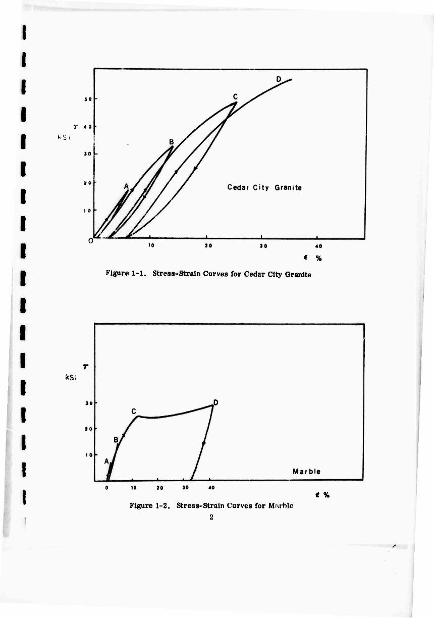
Figs. 1-1 and 1-2 show, respectively, typical stress-strain plots for a

granite and a marble (Swanson 1970). Upon loading the stress-strain curve is

almost linear and reversible over a short portion. Unloading from higher loads

does not coincide with initial loading. This characteristic along with rate inde-

pendence distinguishes elastic-plastic behavior. Reloading closely follows un-

loading until the previous maximum is reached; whereupon the original curve

is followed. This leads to some simplifying assumptions.

1. A yield point exists below which the material is linear elastic.

It, The yield point corresponds to the maximum Htross level previously attained.

iii. Unloading and reloading paths are linear, coin- cident and parallel to the initial elastic loading curve.

Fig. 1-3 shows this simplification. Clearly the yield point can be described by

the permanent or irrecoverable strain or the area bounded by the loading curve,

the unloading curve and the horizontal axis. Whereas in generalization to the

three-dimensional case, the stresses and strains become second rank tensors

and arc, therefore, unordered , the area is still a scalar product and retains

its ordering characteristics. To this extent, it is often preferred as a measure

of the elastic limit.

r «a kS

€ %

Figure l-l. Stress-Strain Curves for Cedar City Granite

kSi

€ %

Figure 1-2. Stress-Strain Curves for Muble 2

Mechanical behavior of rock under polyaxial state of stress has been

oxntnlniMl In Iho light of brittle failure theories (Brace, 1964} Bloniawski, 1907,

19(59; Brady, 1969, 1970). Four regions of behavior are identified in Figure 1-4.

The first region corresponds to closure of pre-existing open cracks and is pecul-

| lar to compressional loading. In region n material behavior is linear elastic.

Fracture initiation occurs near the end of this region in accordance with Griffith

or modified Griffith Theory. This stage also corresponds to onset of nonlinearity

in the stress to volumetric strain curve (Brace, 1966). Stable fracture propaga-

tion characterizes region IL, In region IV, unstable fracture propagation results

in strength failure and rupture. Differences in loading and unloading behavior

are observed (Walsh, 1965).

We have, thus, two general approaches to the characterization of stress-

strain behavior of rock. One follows the theory of elastic-plastic solids without

consideration of micro-mechanics of the system. The other uses Griffith theory

or modifed Griffith theory to relate deformation and failure to initiation and pro-

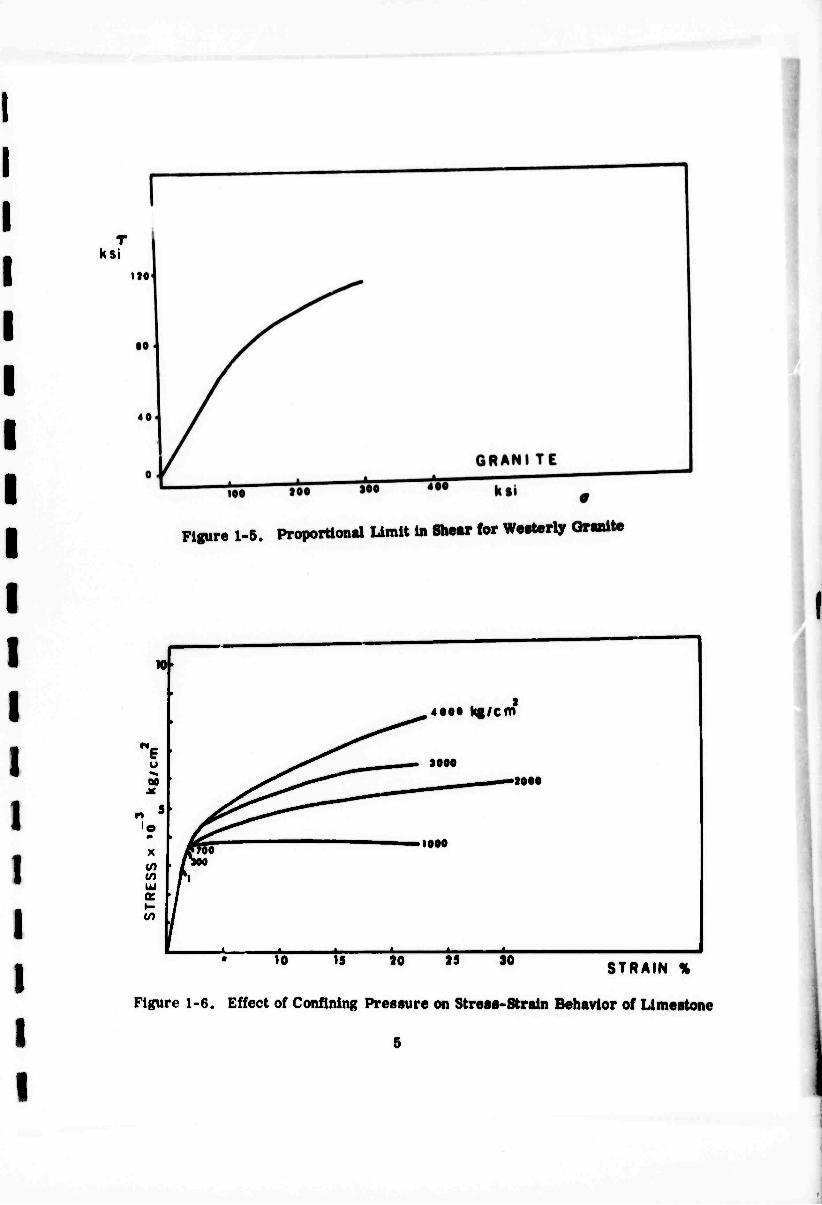
pagation uf fracture. It has been observed (Swanson 1970) that Mohr-Coulomb

failure lav; applies for moderate values of confining pressure and that at low

confining pressures, failure is by rupture. Contrary to plastic behavior, strength

of material drops to almost zero in the direction normal to the crack If rupture

theory is followed. Figs. 1-6 and 1-6 depict typical relationships of failure strength

and post failure behavior in relation to confining pressures. It is reasonable to

assume that the material is linear elastic upto yield or rupture , as the case may

'

%

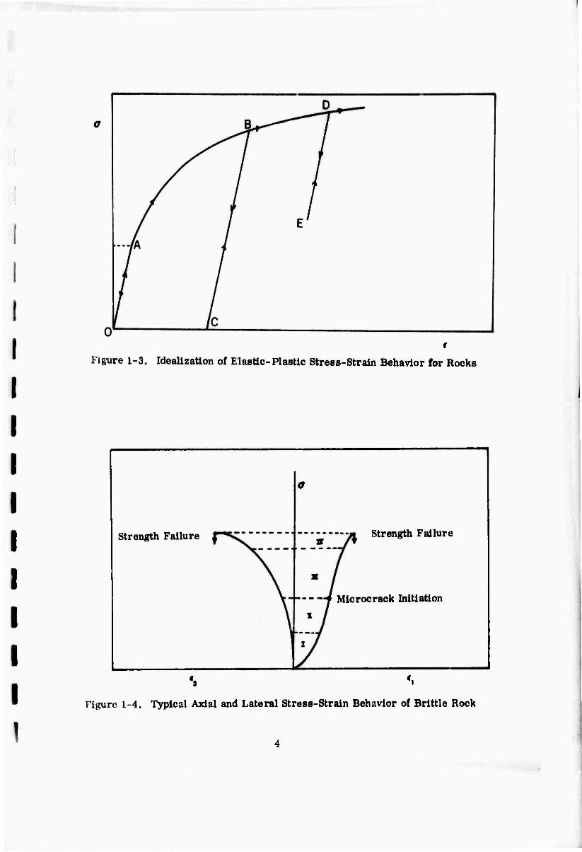
Figure 1-3. Idealization of Elastic-Plastic Stress-Strain Behavior for Rocks

Strength Failure

o

Strength Failure

-f Microcrack Initiation

•3 '1

Figure 1-4. Typical Axial and Lateral Stress-Strain Behavior of Brittle Rock

T ksi

no

Figure 1-5. Proportional limit In Shear for Weeterly Ormlte

KJ i

kg/cm i

f9

|

/ ̂ - sooo

—•r*-

, 3 ' ^^ ̂ ^^—* ̂ ^"^^ 'e

• faZ0^* X JPS*

UJ

/ 10 is 30 23 30 STRAIN %

Figure 1-6. Effect of Confining Pressure on Stress-Strain Behavior of Limestone

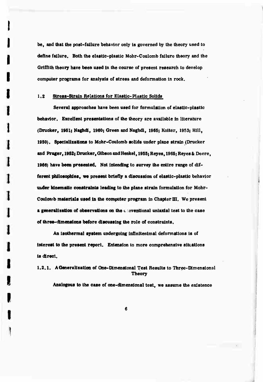
be, and that the post-failure behavior only is governed by the theory used to

define failure. Both the elastic-plastic Mohr-Coulomb failure theory and the

Griffith theory have been used in the course of present research to develop

computer programs for analysis of stress and deformation in rock.

1.2 Stress-Strain Relations for Elastic- Plastic Solids

Several approaches have been used for formulation of elastic-plastic

behavior. Excellent presentations of the theory are available in literature

(Drucker, 1951; Naghdl, 1960; Green and Naghdi, 1965; Kolter, 1953; Hill,

1950). Specialisations to Mohr-Coulomb solids under plane strain (Drucker

and Prager, 1952; Drucker, Gibson and Henkel, 1955; Reyes, 1965; Reyes & Deere,

1966) have been presented. Not intending to survey the entire range of dif-

ferent philosophies, we present briefly a discussion of elastic-plastic behavior

uuder kinematic constraints leading to the plane strain formulation for Mohr-

Coulomb materials used in the computer program in Chapter III. We present

a generalization of observations on the c Aventional uniaxial test to the case

of three-dimensions before discussing the role of constraints.

An isothermal system undergoing infinitetiimal deformations is of

interest to the present report. Extension to more comprehensive situations

is direct.

1.2.1. A Generalization of One-Dimensional Test Results to Three-Dimensional Theory

Analogous to the case of one-dimensional test, we assume the existence

I

of a set D consisting of all admissible states of stress. D is convex,* has boun-

dary B and includes the original or reference state. Clearly D is six-dimensional

(assuming symmetric stress tensors, i.e. absence of body couples) and is con-

tained in the six-dimensional linear vector space V spanned by the six components

o-^j of the stress tensor. The stress in unlaxlal test is given by a real number and

in this case D is ordered and convex. To introduce an ordering In the six-dimen-

sional stress space so that 'increase* and •decrease' of stress are meaningful,

a mapping g is defined

g: V—*R (1-1)

with the following properties

i. The image of D under g is a positive interval I C R.

11. Image of complement of D in V is the complement of I in R and g maps the interior Dj of D to the (1-2) interior of I.

ill. g maps the 'original' or 'reference' state to zero € I.

Then D is ordered by its image i.e. for Uy ^SD, if g(i'i> ■ g}, gO^) = 82* "2 iB

greater than, equivalent*1^, or less than vi depending upon g2 being greater than.

!

«Convexity of D is the property that vi, t^EDafrafi + (1 -a) v^EDYa€ [0, ll. In literature, there are frequent references to a convex yield surface. This is in- accurate. It is easy to see that convexity of D does not imply convexity of its boun- dary B. Indeed, B is in general not convex.

♦♦The term equivalent is used because g, in general, is not one to one. Thus, I/J, 1^2 may be distinct while their images coincide.

equal to or less than g^. The mapping preserves convexity of D. The Interval

1 = [0f f J where f Is the Image of boundary B of D.

In one-dimensional tests, the set of admissible stress states may include

negative points. The limiting stress states in ters'or. and compression provide

a positive supremum and a negative infimum to this set. The boundary B of this

set is clearly discontinuous. In a multi-dimensional stress space, B may be

continuous. To ensure correspondence between the one-dimensional and multi-

dimensional cases, g is a two to one mapping in the case of one-dimensional

loading. Thus the image of B is in all cases the supremum of non-negative

interval I.

The boundary B of D and hence its image f under g are defined by prior

deformation and load history. Considering components e., of the strain tensor,

on the analogy of the results of one-dimensional test, a plastic strain tensor

with components c "^ is defined such that

i. For a given c"kl» there is one to one correspondence between elements of D and a set of points in the six- dimensional space spanned by e 'kl = ekl - e"kl • e 'kl are identified as components of the elastic strain tensor,

(1-3) 11. If a generalization of Prandtl's simplifying assumption

is admitted, the one to one correspondence between "'kl € D an^ e 'kl ^s independent of prior deformation history, and for stress states defined by interior Dj of D, c "kl vanish.

A positive maasure of history of deformation can be defined in various

ways. If plastic strain is used as representative of deformation history, a

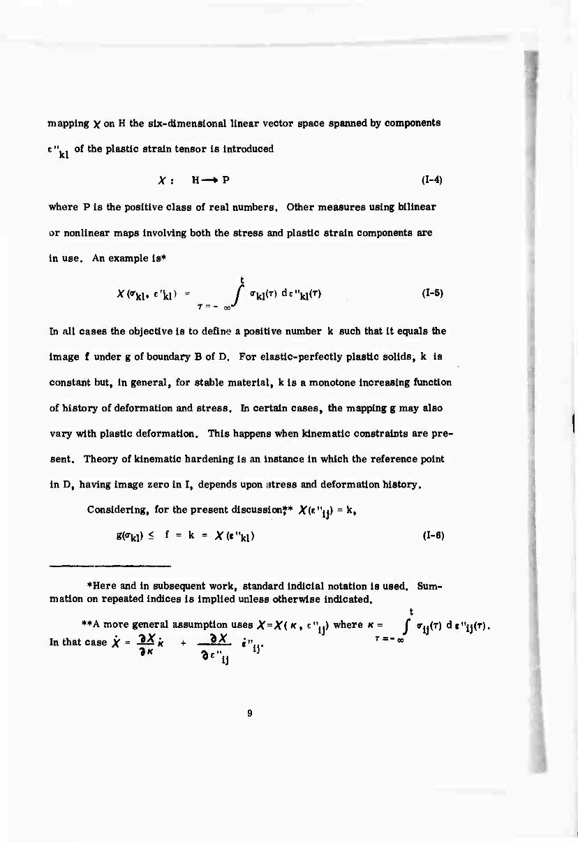
mapping X on H the six-dimensional linear vector space spanned by components

kl of the plastic strain tensor is introduced

X : H- (1-4)

where P is the positive class of real numbers. Other measures using bilinear

or nonlinear maps involving both the stress and plastic strain components are

in use. An example is*

t *('kl. cV - /'<rkl(T)de"

T = - oo*7 klC) (1-5)

In all cases the objective is to define a positive number k such that it equals the

image f under g of boundary B of D. For elastic-perfectly plastic solids, k is

constant but, in general, for stable material, k is a monotone increasing function

of history of deformation and stress. In certain cases, the mapping g may also

vary with plastic deformation. This happens when kinematic constraints are pre-

sent. Theory of kinematic hardening is an instance in which the reference point

in D, having image zero in I, depends upon utress and deformation history.

Considering, for the present discussion** Xte^u) = k,

g(<rkl) < f = k = ^(e-ki) (1-6)

♦Here and in subsequent work, standard indicial notation is used. Sum- mation on repeated indices is implied unless otherwise indicated.

t **A more general assumption uses X=X{ *, e"..) where K = f V^T) d e"ij(T).

In that case X = —* + —%&. i"... Tm~i

2* ^"ij

ir

In the interior of D, r "kj ■ 0, g^^jX f = k and

'kl = Ekl(f,mn)

■ Ekl ^mn> ^^

For differential changes in stress and strain components, using a superposed dot

to indicate differential quantities,

Tkl " Eklmn c,mn

■ Eklmn ^mn <I'8)

assuming that Ekl -s sufficiently smooth and its derivative Ekimn»a tensor of

fourth rank,exists.

On the boundary B of D,

g(<rkl) = f = k = V(c"kl) (1-9)

For g, X sufficiently smooth in their arguments • • •

* = X (e"kl) = hkle"kl (I-10)

g = g(«rkl) ■ Qkl'kl <1-11)

In the case of elastio-perfectly plastic solids, hkj = 0 and arbitrary plastic straining

can occur for X = 0 i.e. X- k, a positive constant. Also g = f = k requires g = 0

leading to the relationship

qki;kl = 0 (1-12)

Equation 1-12 requires the stress changes to be in a plane tangent to the hyperplane

defined by g (or^j) = k. However, for hw / 0,for nonvanishlnge "^j, X > 0 and g = • • • • •

f >0. This is termed loading and g = f = k = X. For vanishing e"^, X - 0 and

10

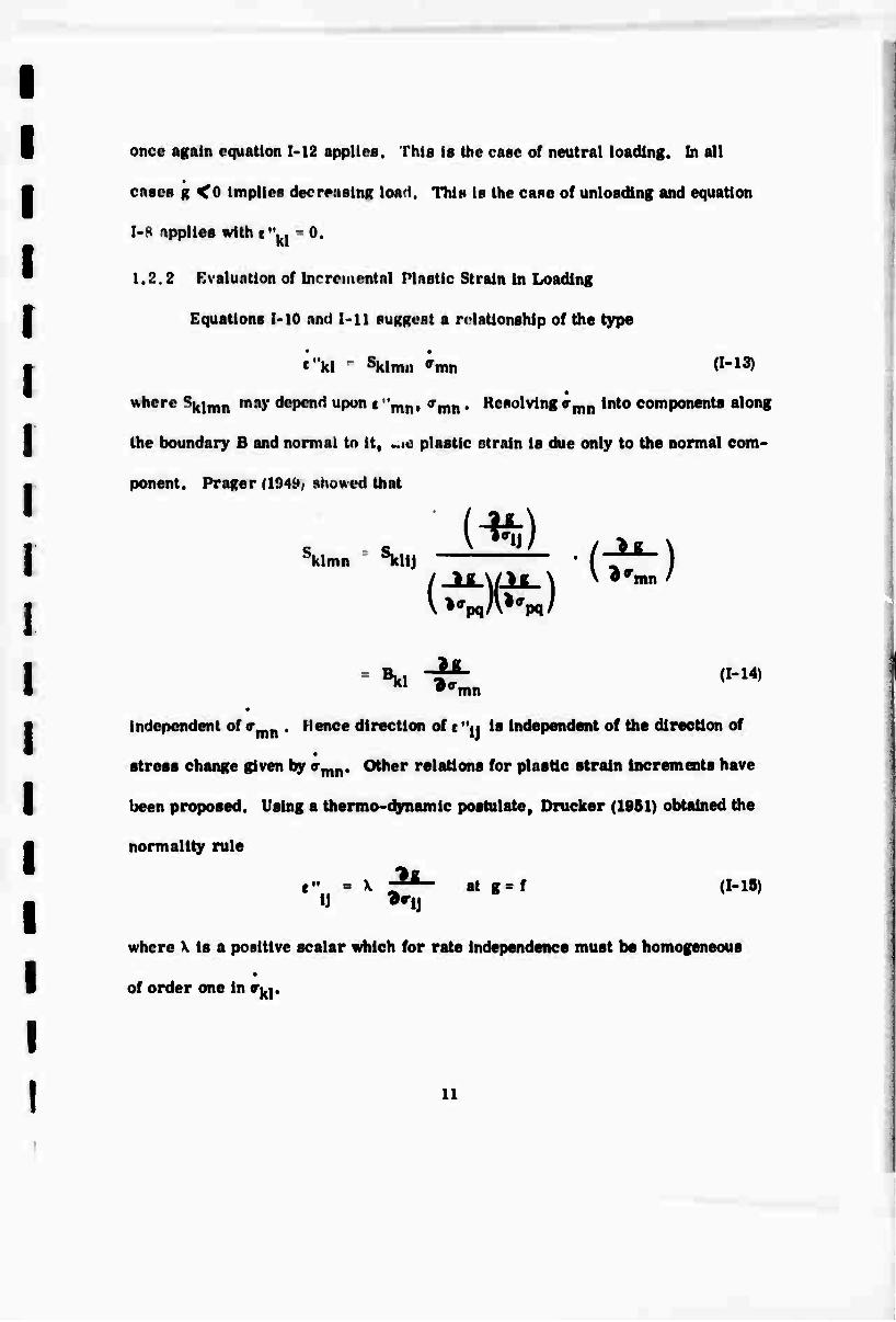
I once again equation 1-12 applies. This is the case of neutral loading. In all

cases g <0 implies decreusing load. This Is the case of unloading and equation

1-8 applies with e'V. ■ 0.

1.2.2 Evaluation of Incremental Plastic Strain in Loading

Equations I-10 and Ml suggest a rolationship of the type

«"kl sklmn »mn (I-13)

where \\mn may depend upon i "mn, Jmn . Resolving <rmn Into components along

the boundary B and normal to it, ..«o plastic strain is due only to the normal com-

ponent. Prager (194i<f showed that

■ •" "Si independent of <rinn . Hence direction of c "M is Independent of the direction of

stress change given by 9mn. Other relations for plastic strain increments have

been proposed. Using a thermo-dynamic postulate, Drucker (1961) obtained the

normality rule

e" = \ ~*— at g=f (1-15) ij ^i,

where X is a positive scalar which for rate Independence must be homogeneous

of order one in <T^.

11

I I I I

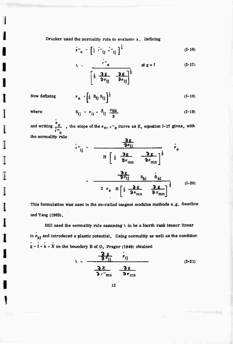
Drucker used the normality rule to evaluate A . Defining

• r" ^ e

'l f" r*II I2 (1-16)

\ = F"e at g= f (1-17)

Now defining <re = h Sy SJJ I8

• 1

(1-18)

where S-. - o-^ - S /kk 3

(1-19)

cr and writing e , the slope of the (ret e "e curve as H, equation I- -17 gives, with

e the normality rule

11. ^"•ii

•

ij ^g ^g -1^

L2 ^mn ^mnj

f g **i) hi skl

. ,i (I"20)

e [ ^mn «^mnj

This formulation was used in the so-called tangent modulus methods e.g. Swedlow

and Yang (1965).

Hill used the normality rule assuming X to be a fourth rank tensor linear

In ir^j and introduced a plastic potential. Using normality as well as the condition I • « * i

g ^ f = k = V on the boundary B of D, Prager (1949) obtained

^L "n <r. \ = z—U (1-21)

^E"mn ^«"mn

12

This formulation breaks down for clastic-perfectly solids where X is independent

mn. Felippa (1966) obtained X in terms of en, increment in the total strain

tensor. In this procedure

Off

'ij I Eljkl ^km ^ln " Eijkl Milmn f mn (1-22)

where Jklmn

[M- Jit + ll_ E 3£- T1 JLß- E .. ^^ l>c"ij &n ^ij ^ ^'pqj ^'rs r8k1'»^ 'mn

(1-23)

This approach is valid for all cases including perfect plasticity and was used by

Zienkiewicz, Valliappan and King (1969) in developing finite element procedures.

Using rate of work equations, it is possible to evaluate X in terms of stress

rates for materials of von Mises or Mohr-Coulomb type. Yamada (1968) used this

approach for finite element analysis of von Mises solids. Using Drucker and Prager's

generalization of Mohr-Coulomb law, Reyes (1965) developed the stress-strain equa-

tion for generalized Mohr-Coulomb elastic-perfectly plastic solids under plane

strain conditions. The finite element procedures presented by Reyes and Deere

(1966), Baker, Sandhu and Shieh (1969) and those included in Chapter III of this

report were based on these equations. For plane strain

11

r22l

12

= 2G

Dll D12 D13-| ell

D21 D22 D23 «22

D31 D32 D33J ^12

(1-24)

where Dll = 1 - h2 - 2 hi <rii - ha vu*

D22 = 1 - h2 - 2 hj 0-22 - l^ ir222

13

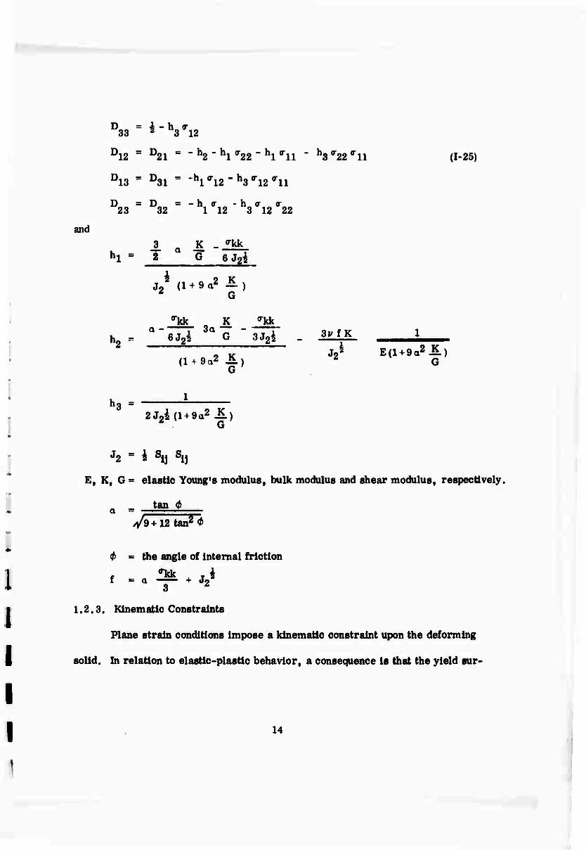
and

D33 = *-S'ü D12 = D21 = ' h2 ' hl'22 " hl'11 " ^^'ll (1-25)

D13 * D31 = -V^-^'^'ll

D =D =-h(r -ho- v 23 32 1 12 3 12 22

hl = 2 G 6 J2i

J2 (1 + 9 a2 -£ ) Z G

'kk K ""kk a r 3a T -

h0 P 6J2i ^ G 3J2^ . 3vfK '2

■ E(l + 9a2iL) (1 + 9a2 Ü) 2 "^•-"- G

hg = 232h. (l + 9a2 ii)

J2 = i Slj S1J

E, K, @ ■ elastic Young's modulus, bulk modulus and shear modulus, respectively.

„ _ tan 0

//9+12 tan2*

0 ■ the angle of internal friction

f = a -^ + J2i 3 Z

1.2.3. Kinematic Constraints

Plane strain conditions impose a kinematic constraint upon the deforming

solid. In relation to elastic-plastic behavior, a consequence is that the yield sur-

14

I

I I

surface from the elastic side iid plastic side do not, in general, coincide (Baker

et.al. 1969). Consider the deformation of a body undergoing deformation. F, the

set of all admissible deformation, is contained in the six-dimensional vector

space S spanned by components rui of the strain tensor. A kinematic constraint

can be written as

C (Ckl) = 0 (1-26)

and the admissible deformation is restricted to the intersection of F with the hyper-

plane in S defined by equation 1-26. If several constraints are present, the admiss-

ible deformation is restricted to n n K (<ki) = o] (1-27)

As the multiple intersection reduces the dimension of the vector space by n, it is

clear that n cannot exceed six.

Consider a single constraint. In differential form the equation is

CW cid = 0 (1-28)

where coefficients C^ depend upon e^.

As elastic-plastic behavior is studied with reference to loading paths in

the stress space V, it is necessary that kinematic constraints be rewritten as

constraints on stress. Here, for no plastic strain, we simply use the Inverse of

equation 1-8 to write equation 1-27 as

ckl cklmn 'mn = 0 (J"29)

Gmn 'mn = 0 &*)

15

where Cklmn = [Eklmnl'1 <I-31)

*** Gmn " ckl cklmn <1"32)

For the case of not all of r "^ vanishing, two alternative procedures are available.

Using definition of elastic strain tensor,

ekl = * 'kl + * \\ V-33)

If T, ij-- is the inverse of \imn in equation 1-13

• • • Ekl = cklmna'mn+Tklmn'mn (I'34)

= [^Ipq + Tklmn EmnpqJ £ 'pq (I"35)

- »w« l'« <I-36)

where IM^. IS a four'Ui rank identity tensor. Thus the constraint is expressed by

C.. c,, = C.. K,. c' (1-37) kl kl kl Tclpq pq • ^

" ckl KklpqCpqmn'mn (1-38)

^klmn'mn^ ^

Jklmn = Ckl [^pq + ^Irs Erspq J Cpqmn (I'40) where Lklmn = Cl

An alternative procedure is to use the normality rule and to satisfy the constraint

both upon loading and unloading i. e. Ckl e 'kl = 0 = ^kl e "kl • Then the fir8t e(Iua~

tion is identical with equation 1-29 but the second equation gives

ckl x •^-fi- " 0 (1-41) «'kl

Equation 1-41 may or may not coincide with equation 1-39. Equations 1-29 and 1-39

have linear relationship between incremental stresses and describe hyperplanes

tangent to any loading path in the stress space V. As the two equations are in

general different, there is a slope (.iscontinuity in the stress path as plastic

straining begins upon reaching the boundary B of D. We note In particular that

proportional stress paths in V may not be possible in the presence of kinematic

constraints. In the case of linear elasUclty( let equation 1-30 define a plane

passing through the origin in V. A proportional loading path lying In this plane

is possible upto the point of intersection with boundary B. Beyond that, upon

loading, stress path has to be in the surface determined by Equation 1-39 and

this will in general be non-planar. If loading Is continued to a certain point

along this surface, unloading therefore wilt be along a path lying in a plane

parallel to the original loading plane but different from it and not passing through

the origin. Thus unloading to Initial state is impossible. This corresponds to

setting up of residual stresses corresponding to kinematic constraints.

Specifically considering plane strain conditions and elastlc-perfectly

plastic Mohr-Coulomb material, the mapping g from the set of all admissible

stress states to the positive Interval [o, f ]ls

g (o-y) = a — ♦ Jg2 (1-42)

J2 = i 'ij 'Ij " — (I"43)

Linear Isotropie elasticity implies, for r "JJ ■ 0

Plane strain condition implies

c13 " c23 = e33 " 0 C1"46)

17

From equations 1-44 and 1-45

'13 " '23 " ü <1-46)

'33 = 'fll + 'ii (I-47)

| u For t ji, not all vanishing, using normality rule

. " x U IiLlX-LiiIhL.1 eij = xl3 ^ —n^ J «Ttk

■ 0 a + '33 " 3 3

2 J2i

2 S

2 a Joi '33 - - —f-

'11 + <r22 + —————

or (Tgg- -a J25 + !(••!!+••22) (1-48)

Equations 1-47 and 1-48 define different surfaces in a three-dimensional space

spanned by 0-^, o^t 'ss* L^ their intersections with B be respectively, P and

Q. The stress path is constrained to lie in the plane defined by equation 1-47 for

stress states in the Interior of D and for neutral loading. For plastic deformation

to occur the stress path must lie in the surface defined by equation 1-48. For a

continuous stress path to be possible, P and Q must coincide. In general this

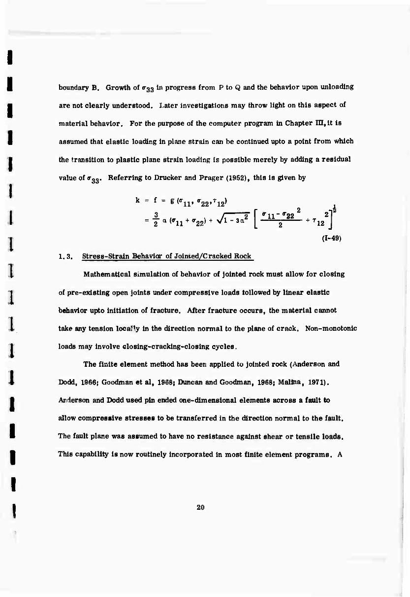
is not the case. Figure 1-7 illustrates the difference between the surfaces P

and Q for Mohr-Coulomb plane strain case.

Considering that the stresses 0-33 do not contribute to energy/work of the

system, it appears reasonable to assume that progress from P to Q is possible

with gradually increasing the value of 0-33. This would amount to following the

1«

1

cd 1 V o

u 1 •o Pk >s | g P

<M

I

cd

j TB ü

i I u u ja o

5 a

0)

i

i

19

I

boundary B. Growth of 0-33 in progress from P to Q and the behavior upon unloading

are not clearly understood. Later investigations may throw light on this aspect of

material behavior. For the purpose of the computer program in Chapter in,it is

assumed that elastic loading in plane strain can be continued upto a point from which

the transition to plastic plane strain loading is possible merely by adding a residual

value of 0-33. Referring to Drucker and Prager (1952), this is given by

k - f - g ^U( <r22,T12) 2 af

(1-49)

I i ' f ' ('U * '22> ^ v/l - »°2 [ '" 2 * T12 J

I 1 I I

1.3. Stress-Strain Behavior of Jointed/Cracked Rock

Mathematical simulation of behavior of Jointed rock must allow for closing

of pre-existing open joints under compressive loads tollowed by linear elastic

behavior upto initiation of fracture. After fracture occurs, the material cannot

take any tension loca?ly In the direction normal to the plane of crack. Non-monotonic

loads may Involve closing-cracking-closing cycles

The finite element method has been applied to jointed rock (Anderson and

Dodd, 1966; Goodman et al, 1968; Duncan and Goodman, 1968; Maltna, 1971).

Anrlerson and Dodd used pin ended one-dimensional elements across a fault to

allow compressive stresses to be transferred in the direction normal to the fault.

The fault plane was assumed to have no resistance against shear or tensile loads.

This capability is now routinely incorporated in most finite element programs. A

20

two-dimensional 'soft' material element has long been used to represent weak

joint planes in rock. Duncan and Goodman ^1968) object to this on the basle of

large number of elements needed to ensure a reasonable 'aspect ratio' In Hhupe

of elements. This becomes a problem for elements representing very thin JolnlH.

A one-dimensional element with shear and normal stiffness characteristics was

proposed by Goodman et al (1968) to eliminate this objection. Recently (1971),

the same investigators have introduced nonlinear properties in this type of ele-

ment. This approach is quite effective for the case of pre-existing joints in rock.

For well defined orthogonal joint systems, an orthotropic continuum approach

was suggested by Duncan and Goodman (1968). Christian is credited (Einstein,

Bruhn and Hirschfeld, 1970) with development of an element capable of simulating

constant shear and residual shear characteristics.

In all these investigations, a distinct set of elements is used to represent

the joint. This is alright for pre-existing joints but is impracticable for dis-

continuities arising as a result of fracture under applied load. To use the same

procedure both for pre-existing joints as well as post failure cracks, it is nec-

essary to allow cracks and joints within elements. Then, the mesh layout is

more flexible and arbitrary failure laws can be used. Malina (1971) used this

approach to study failure along joint planes and then went on to compute the

amount of slip and accompanying stress redistribution on the basis of deforma-

tion or slip theory of plasticity.

21

Apparently, a blmodular analysis procedure (Sandhu and Wilson, 1970)

can be used to represent pre-existing joints as well as fractures. Bimodularity

would be dependent upon the joint opening. However, noting that fractured or

open jointed rock has no resistance to tension in the direction normal to that of

fracture, a simple approach following the procedure introduced by Zlenkiewicz

et al (1968) is more convenient. The 'no tension' method of Zlenkiewicz consists

of first obtaining a solution assuming the system to be linear elastic. Then the

elements in tension are rel.aved of the tensile stresses by application of self-

equilibrating forces in elements and at nodal points. This gives an iterative

scheme for redistribution of loads to surrounding rock and a lower bound to

the exact solution. This approach is essentially an orthotropic continuum

approach with the orthotropy being applied to Individual elements depending

upon the orientation of the fracture plane. The fracture plane defines also a

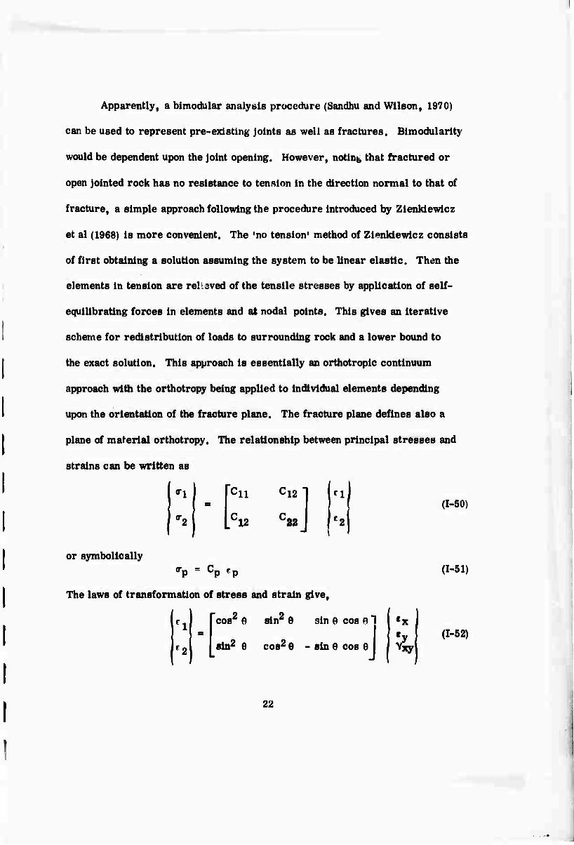
plane of material orthotropy. The relationship between principal stresses and

strains can be written as

""l

*2

Cll

C12

Cl2

C22

El

C2|

(1-50)

or symbolically ^P = Cp Ep (1-51)

The laws of transformation of stress and strain give.

f2l

cos2 0 sin2 6 sin e cos 01

sin2 6 cos2 6 - sin 6 cos 6 J Yxyl (1-52)

22

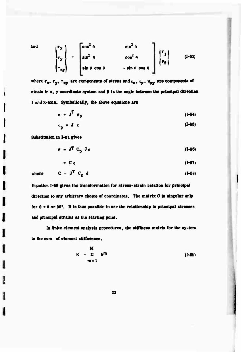
and

xy

" 2 cos n »In2 n i

■In2 o cos2 ft

sin ft cos ft - sin o cos ft

(I-B3)

whcru vx, (T ijjy are components of stress and cx. Cy, >_ are oompooents of

strain In x, y coordinate system and 0 Is the angle between the principal direction

1 and x-axls. Symbolically, the above equations are

T

.p-J.

(1-54)

(I-6B)

Substitution In I-Sl gives

T - jT C J e (I-B6)

Ce (I-B7)

where C ^ JT Cp J (1-68)

Equation I-5ft gives the transformHtton for streas-strain relation for principal

direction to any arbitrary choice of roordlnatcs. The matrix C Is singular only

for ft - o or 90*. It Is thus possible to use the relationship In principal stresses

and principal strains as the starting point.

In finite element analysis procedures, the stiffness mxtrix for the system

is the sum of element stiffnesses.

M

K = Z km

m = l (I-Oll)

23

where K Is the system stiffness, km is the stiffness of the nth element, and E

is viewed as a direct stiffness summation operator. Further, element stiffness

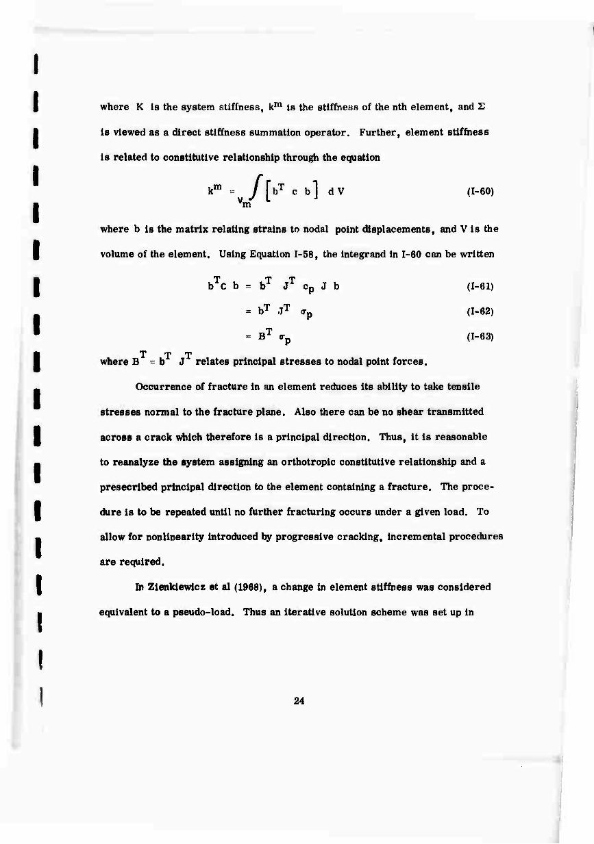
is related to constitutive relationship through the equation

km - /[bT c b] dV vm

(1-60)

where b is the matrix relating strains to nodal point displacements, and V is the

volume of the element. Using Equation 1-58, the integrand in 1-60 can be written

bTC b = bT JT Cp J b (1-61)

= bT JT o-p (1-62)

- BT (rp (1-63)

X T X where B = b J relates principal stresses to nodal point forces.

Occurrence of fracture in an element reduces its ability to take tensile

stresses normal to the fracture plane. Also there can be no shear transmitted

across a crack which therefore is a principal direction. Thus, it is reasonable

to reanalyze the system assigning an orthotropic constitutive relationship and a

presecribed principal direction to the element containing a fracture. The proce-

dure is to be repeated until no further fracturing occurs under a given load. To

allow for nonlinearlty Introduced by progressive cracking. Incremental procedures

are required.

In Zienklewlcz et al (1968), a change in element stiffness was considered

equivalent to a pseudo-load. Thus an iterative solution scheme was set up in

24

which each iteration only Involved a back-substitution operation. The pseudo-

loads were computed as equivalent to tensile principal stresses. This is satis-

factory when both principal stresses are tensile. However, when only one of

the principal stresses is tensile, use of pseudo-load corresponding to one prin-

cipal stress introduces a non-symmetric constitutive law. Actually if the phy-

sical concept of 'unloading without any displacements• be followed, a change in

the second principal stress corresponding to Poission's effect due to the first

stress must be included. This modification is included in the computer program

in Chapter IV.

25

I I

CHAPTER n

THE FINITE ELEMENT METHOD

4^

Chapter II. The Finite Element Method

2.1. Basic Concepts

A boundary value problem can be stated in the form

A u = f on F (H-l)

where u is the unknown function to be determined, A is an operator, and f is the

'forcing* function. F is the domain of interest and may be an open, connected,

bounded spatial region embedded in R or in a cartesian product, R x fo, »)

where fo, ») is the non-negative time interval. In addition to the field equation

n-1, there will be some conditions to be satsifed on boundary S of F. For A

linear positive, it can be shown that equation n-1 has a unique solution. Nec-

essarily, any approximate solution will in general not coincide with the unique

solution of n-1 and consequentl; no approximate solution is expected to satisfy

the field equation as well as the boundary conditions completely.

Solutions to engineering problems as well as the forcing functions are

in general bounded and therefore belong to Lg »the space of square Integrable

function. However u may be contained in a subset D of Lo such that A is defined

on D. We assume that D is dense in L^. If the set of functions | ^ k= 1,2,.. «X

is an orthonormal basis in D, then any function u can be expressed as an Infinite

sum: N u = Z ak tfk ai-2)

k = l

A scheme to generate approximate solutions is to use a finite set of terms in the

26

infinite sum above. Thus, we use N

S s ks i ak ^ (n-3)

as an approximation. The approximation process then consists of appropriate

choice of N, (/^ and the coefficients a^. Several alternative procedures are avail-

able. The finite element method is a special process of selection of a finite sub-

set of the basis { ^uf • The coefficients a^ are evaluated by an extension of Ritz

method or other standard procedures.

The finite element method is well documented In literature (Zienkiewicz,

1967; Bell andHoland, WPAFBConference, 1965,1968; Felippa, 1966;Clough, 1960,

1965). Its theoretical basis (Oden, 1969; de Arantes e Ollveira, 1968, Zlamal,

1968; Melkes, 1970) and relationship to variational principles (Melosh, 1963, Plan

and Tong, 1969) have been examined. Essentially, a finite element Idealization

partitions the spatial region F into a finite number of nontrivial discrete elements

or subregions. The geometry of the elements Is defined by a set of points in space

called the nodal points of the system.

Over an element e let an approximation to u be Ne

.e «. „ e ä e

or in matrix form

-rekT

uB = S ake \v (n-3)

k=l

ue = [r f { a6} (n-4)

where { 0 | is a row vector consisting of \e as its elements and |ae|is a

27

column vector of coefficients a^6. Evaluating the function at nodal points

«. T

(n-6)

where | uj61 is the vector of nodal point values of the function andj^i | is the

matrix of base functions evaluated at each nodal point. Rows and columns off^i 1

are linearly independent. If square, the matrix is invertible. If the number of

nodal points is not equal to the number of independent base functions, a least

square procedure can be used for inversion. Hence, we can write

{•e}= [mT1 M

Substituting n-6 in 11-5 T

ue = { *e} [A] -1 | ut6 | (n-7)

*\**f hf] (n-8) where | ^ i can now be regarded as a set of interpolating functions relating nodal

point values of a function to the value of an arbitrary point within the element.

2.2. A Potential Energy Formulation

We HKRump th« rock continuum or •discontinuum1 to be stepwise linear for

Mufflrirnilv 'null rit«pn In loading. For such a case the governing equations are

'ki.k ' ".k Nk * p Fi

'ij Eljkl «kl ' 'ij

ekl u(k,I)

= 0 (II-9)

(11-10)

(n-ii)

28

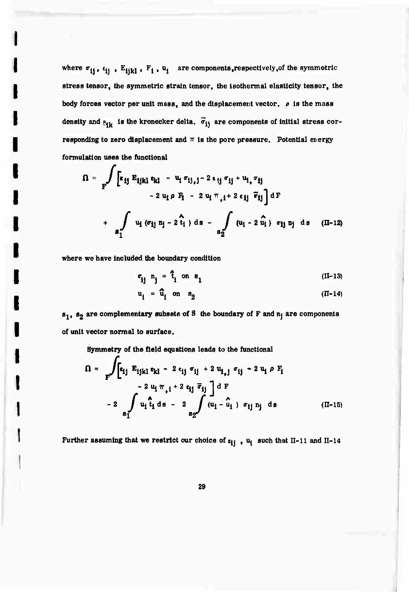
where o-j., cj. , E^ t F^ , Uj are components,respectively,of the symmetric

stress tensor, the symmetric strain tensor, the isothermal elasticity tensor, the

body forces vector per unit mass, and the displacement vector, o is the mass

density and f». is the kronecker delta, ö-js are components of initial stress cor-

responding to zero displacement and n is the pore pressure. Potential ei ergy

formulation uses the functional

n - /[. 1J Eljkl «kl " ^ ""ij»!" 2 Mj 'ij + % 'ij

2uipFi - 2 Ui7r(j+2 ey iy j dF

f h f * J uj (O-JJ nj - 2 tj ) ds - I (ui - 2 uj) o-y nj ds (11-12) +

BZ 8

where we have included (he boundary condition

o-. n. = t. on s1 (11-13)

u. = Uj on s« (11-14)

s1, 82 are complementary subsets of S the boundary of F and nj are components

of unit vector normal to surface.

Symmetry of the field equations leads to the functional

-2uj7r 1 + 2Ejjö:ij|dF

r A f * I ujtids - 2 I (uj - uj ) crjj nj ds (11-15)

•f B2r -2

Further assuming that we restrict our choice of q« , 14 such that 11-11 and 11-14

29

arc identically sutlsflcd, the functional In 11-15 reduces to

" J Kj Eijkl uk,l - 2uip Fi - 2^ 7rji+ 2 U^J^J I dF

- 2 / Ujti ds (n-16)

./

m /_ -.m Replacing / by S Jm where F represents the subregion or element

m, and using suitable interpolation scheme to express the integrand in terms of nodal

point vectors of displacement, vanishing of variation of the functional yields the matrix

equation

HI" m

where

[K]|ut . jR| m _

[K]. Z „- m = l J

(11-17)

(n-18)

|Rt = ■.f.[M + Pm - Qm hM] (n-i9)

Components of element stiffness matrix and load vectors are:

klJ - / Fm

. m nm.n Emnpq 0JP.q (11-20)

L.». /m

j.m _ P ^ij f) (n-2i)

nm' fm *ij ^.J (n-22)

m 0, =

pm

m _ im,n 'mn (n-23)

m Ti = ^m

(11-24)

I

_ rp

and I'ft are components of a matrix formed by the row vectors | <t> \ corresponding

to each degree of displacement freedom. The vectors |Lm|, jPmj, {Qm |, |Tm}

represent the contribution to the load vector made respectively by the body forces,

the pore pressure gradients, the initial stresses and the boundary loads in the ele-

ment m.

2.3 Incremental Analysis

In case of Incremental construction and incremental application of loads,

the loads, stresses and displacements for any incremental step can be written as

|Rn} • {"nl and |un| • Then for the next stage, |(rn| and |un| can be regarded

as the initial stresses and the initial displacements for the structural system. Thus

the matrix equations are

[^l] {Vl - un} = [Kn+l]{Aun} = {ARn} <n-25)

where m ARn " s

m = l [AL™! + !APmj - JAQmj + LT1"! 1 (n-26)

and {AL"1! t | APml ,| AQm \ , I A Tm i are increments in the respective quantities.

For elastic-plastic analysis, the stiffness depends upon stress and has to be

re-evaluated at small increments of load. To ensure manageable computation, the

increments are kept at the largest practicable without loss of accuracy.

31

CHAPTER m

COMHJTRR PROGRAM FOR PLANE STRAIN ANALYSIS OF ELASTIC-PLASTIC MüHR-COULOMB MATERIALS

51^

i

Chapter 111. Computei :■■. gr m Plane Strain Analysis of Elastic-Plastic Mohr-Coulomb Materials

3,1, Organization

Computer pro^nrn ^cmribci her.' is based on the theory presented earlier

In ihis report. The program is written in Fortran IV language.

The program is Intended 10 calculate strobes and strains for a plane strain

problem in rock mechanics. Mohr-Coulomb yield criterion has been used. It

makes allowance for the boundary conditions, renldual stresses, stresses due to

temperature change, and varying pressure boundaries. The structure may consist

of different materials. It uses Wilson's (1965) quadrilateral elements and generates

stiffness in line with the integration procedures discussed by Fellppa (1966).

The principal program called MAIN controls all the data Input and control

information. It doeb the basic system initialization and prints the control data and

material and geometrical properties of the structure. Stiffness formulation, equa-

tion solving and stress calculations are done by the subroutines called by MAIN.

3.12. Stiffness and Load Matrices

Stiffness matrix for each analysis It competed in blocks by the subroutine

STIFF. For the element stiffness it calls QUAD for triangular and quadrilateral

elements which have been allowed by this program. The element stiffness is added

to the total stiffness using the direct stiffness technique. Concentrated loads are

included in the load matrix. Equations are modified for the displacement boundary

conditions by calling subroutine MODIFY. For the stress-strain matrix QUAD

32

calls STHSTH. With Ihe cnnstuuuvc law ouln^ iviUlabU«, stiffness of the system

:iml lend matrix an* contpuieil in un- BT1FI HUbruutine.

S, 13. Calculations of Displacemeias

After the stittnes? trul load matrices for a stage have been computed, the

rcsalfnc equations are solved by c illir.g subroutine BANSOL. This uses Gaussian

•limlntttOB technique tor banded equations by Wilson (1963). In this the trlangularl-

Batton of stiffness matrix Is done. Back substitution through the trlangullzed matrix

joves the solution.

3.14. Calculation«« "• Stresses

• i. thi- brat cyeli ■ purely eltattfl solution is obtained for the problem by solving

[K^j{r| {K| (m-l)

whrr- (K* J IS ft« elutte stiffness j r } is tho diS}-;ao.tricnt vector jR | Is the load vector.

This on be done easily by assumine all the tUrfttfll to be elastic to begin with.

As the problem is a nonlinear one, therefore this solution will not be correct. In

our analysis the system is assume:) to t>e stepvnse linear between the yielding of

one element to the other. This is UMlMd not »o cause any significant error. In

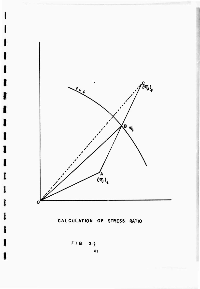
FiR. .1-1 point A represents the Initial stresses and C the final stresses in an ele-

ment. The curve f k represents t>-.e yield surface. For t'.iose elements which

become plastic under this loading AC meets the nurface f k at pt. B. It Is seen

• •.i.sii.v thai for the element it is not possible UJ I.P IOMM to po'.nt C but It can be

loadad to point B only, assuming proportional loading.

33

I

Lot S j ii . H is calloii Ihu HtrcHH ralio. To CMlculatt' S wt-

know that _* AC - ((Tjj), - (-rjj ij

OB - O^ Ä"B

OA ♦ 8, ' AC

As the point B lies on the yield surface f • k

From equation (111-2) the value of B_ can be calculated, This stress ratio repre-

sents the fraction by which the increment in ptress is to be scaled to bring the final

load on the yield surface.

Value of Sr is calculated for all the elements. The element in which the

final stress state is farthest from the yield surface will have the minimum stress

ratio. If we scale do*ii the displacements and stresses in this ratio, we shall have

the stresses and strainr precisely at the point when the system has its first element

Just going into the plastic region from purely elastic system.

In the next step the element having stress ratio equal to the minimum value

is assumed to be plastic. To economize on computer time all such elements which

have their value of stress ratio in the vicinity of minimum were also allowed to go

plastic. As the stress-strain matrix if. knowr. th«- stiffness is calculated again and

equation [Ki J I'1} " I Rl} (m":,)

34

is solved. This procedure is repeated until the whole load has been applied to

the system and cumulative stresses and displacements calculated. The stresses

in (i-l)th step become the initial stresses for ith step.

I

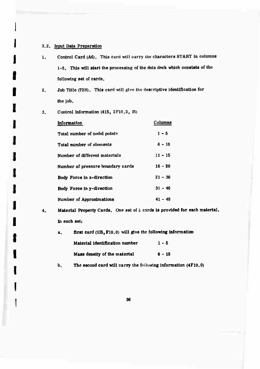
3.2. Input Data Preparation

1. Control Card (A6). This card will carry the characters START In columns

1-5. This will start the processing of the data deck which consists of the

following set of cards.

2. Job Title (72H). This card will give the descriptive identification for

the job.

3. Control Information (415, 2F10.2, If^

Information Columns

Total number of nodal points 1-5

Total number of elements 6-10

Number of different materials 11 - 15

Number of pressure boundary cards 16 - 20

Body Force in x-directlon 21-30

Body Force in y-direction 31-40

Number of Approximations 41-45

4. Material Property Cards. One set of 8 cards is provided for each material.

In each set:

a. first card (lI5tF10.0> will give the following information

Material identification number 1-5

Maas density of the material 6-15

b. Tho second card will carry the foUowlng information (4F10.0)

Information Columns

Elastic Modulus 1-10

Poisson's Ratio 11-20

Cohesion 21-30

Friction Angle in Degrees 31-40

5. Nodal Point Cards (15, F5.0, 5F 10.0».

One card for each nodal point with the following information:

Nodal Point number 1-5

Type of Nodal point 6-10

X-ordinate 11 - 20

Y-ordinate 21-30

XR 31 - 40

XZ 41 - 50

If the number in columns 6 - 10 is

Zero XR is the specified X-load and XZ is the specified Y-load

1 XR is the specified X-dispiaccment and XZ is the specified Y-load

2 XR is the specified X-load and XZ is the specified Y-dlsplacement

3 XR is the specified X-dispIacement and XZ is the specified Y-displacerm

All loads are considered to he total forces acting on an element of unit thickness.

Nodal point cards must be in numerical sequence. If cards are omitted, the

omitted nodal points are generated at equal intervals along a straight line between

the defined nod:,! points. The type of the nodal point, as well as XR, XZ, are set

equal to zero.

37

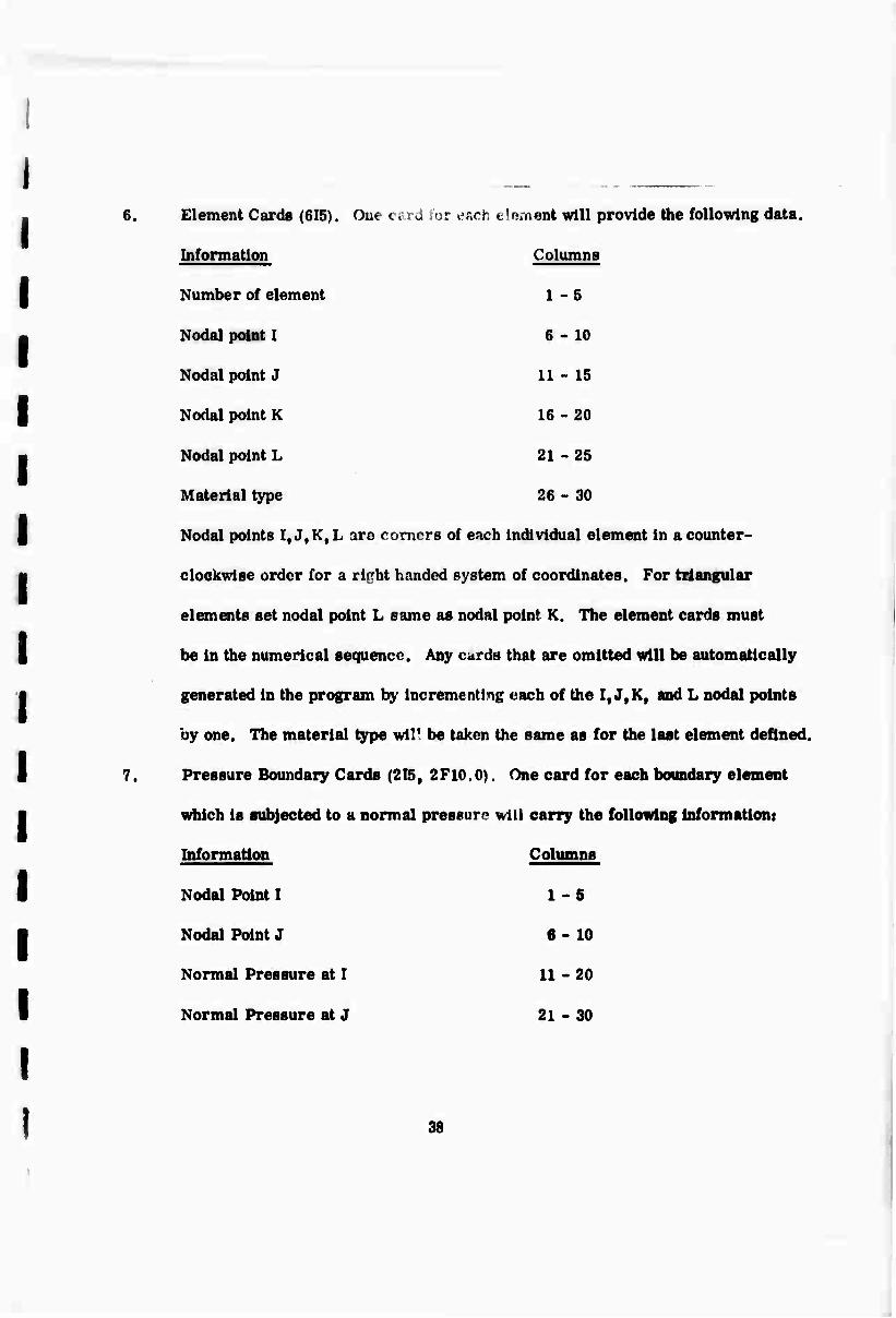
6, Element Cards (615). Out card tor each ele.nent will provide the following data.

Information Columns

Number of element 1-5

Nodal point I 6-10

Nodal point J 11-15

Nodal point K 16-20

Nodal point L 21-25

Material type 26 - 30

Nodal points I, J,K,L arc comers of each individual element in a counter-

clockwise order for a rirrht handed system of coordinates. For triangular

elements set nodal point L same as nodal point K. The element cards must

be in the numerical sequence. Any curds that are omitted will be automatically

generated in the program by incrementing each of the I,J,K, and L nodal points

by one. The material type wir be taken the same as for the last element defined.

7. Pressure Boundary Cards (2T5, 2F10.0). One card for each boundary element

which is subjected to a normal pressure will carry the following information:

Information Columns

Nodal Point I 1-5

Nodal Point J 6-10

Normal Pressure at I 11-20

Normal Pressure at J 21-30

As shown in the sketch, the boundary element must be on the left as one

progressfis from I to J. Surface tensile forces is input as a negative pressure.

Output Information:

The following information is developed and printed by the program:

1. Reprint of input data

2. Nodal point displacements

3. Stresses at the cenior of each clement

39

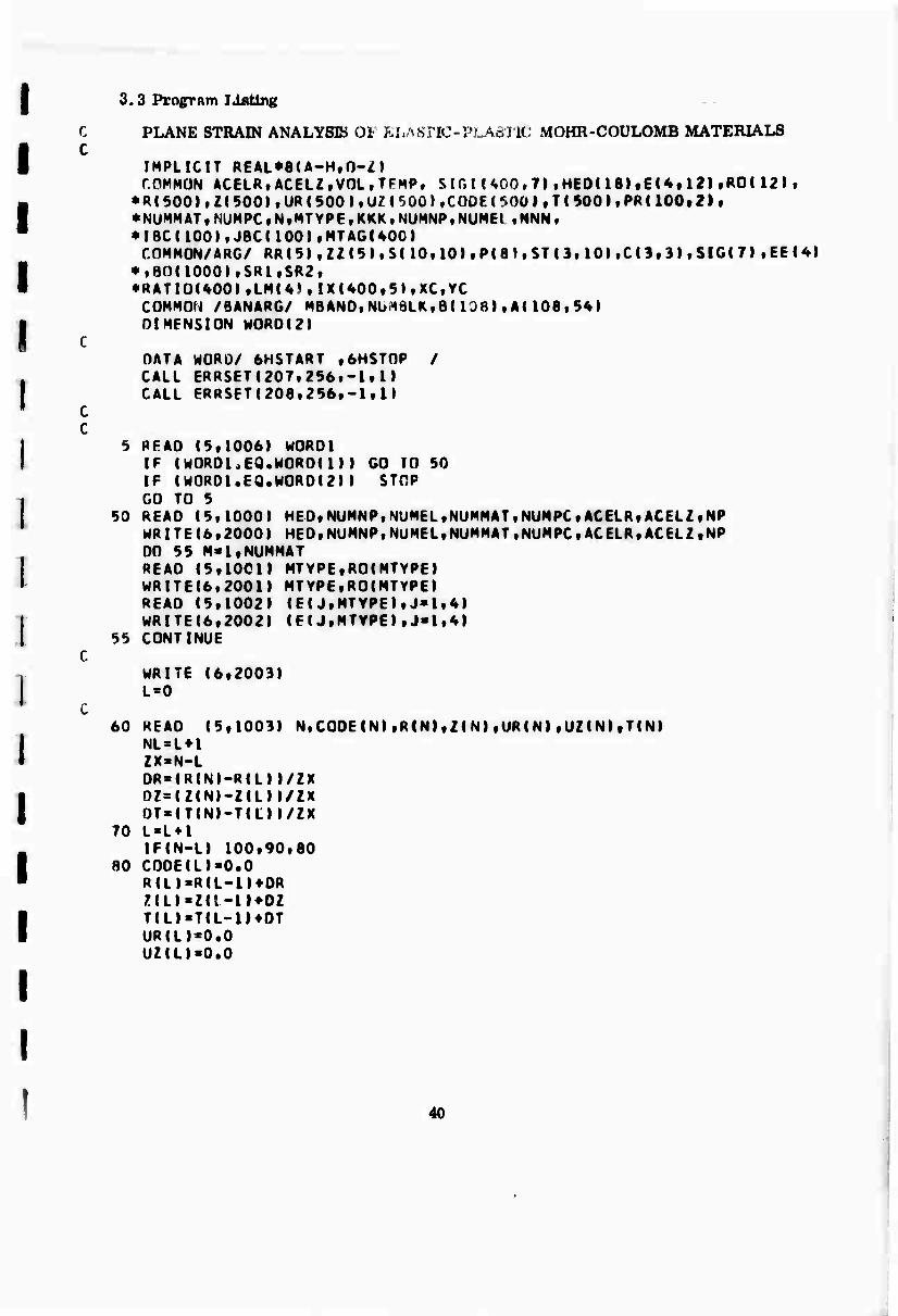
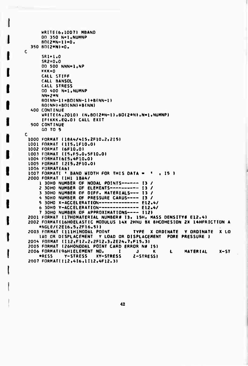
3.3 Program lintlng

C PLANE STRAIN ANALYSE 01 ELASTK-PLASTIC MOHR-COULOMB MATERIALS C

IMPLICIT REAL*8(A-HtfW) r.OMMÜN ACELRfACELZtVOLtTFHP, S If. K ^00 , 7) «HED( 18) tEU( 121 tRO( 12 ) t

*R(500)»Z(500)tUR(500)fUZ(500)*Cn0E(^0Ü)tT(500)tPRn00t2lt *NUMM ATt NUHPC t N «MT YPE « KKK»NUMNP t NUMEl •NNN» ♦ I8C ( 100), JBCl 100) «MTAGUOO» COMMON/ARG/ RR( 5) ,ZZ I 5 ) * S( 10» 10 ). P(8 «, ST ( 3, 10) »COt 3 ) t SIGf 7 ) tEE(4)

*»BOI1000)«SRlfSR2f ♦ RAT10(A00),LM(4SIX(400,5»,XC,YC COMMON /BANARG/ MBANDtNbMBLK,B(138).AlL08t34) DIMENSION W0RD(2)

C DATA WORD/ 6HSTART «6HST0P / CALL ERRSET(207«256»-1«1) CALL ERRSET(208»256f-l,l)

C C

I

5 READ (5*10061 W0R01 IF CMORDl.EQ.MOROm) GO TO 50 IF (W0RD1.EQ.W0R0(2)) STOP GO TO 5

50 READ (5,1000) HED*NUMNPVNUMEL,NUMMAT*NUMPC,ACELR*ACELZ,NP WRITE(6,2000) HED,NUMNP*NUMEL«NUMMAT«NUMPC,ACELRfACELZfNP DO 55 M'ltNUMMAT READ (5»100l) MTVPE«RO(MTYPE) WRITE(6,2001) MTVPE,RO(MTYPE) READ (5,1002) (E(J,MTYPE)♦J»1,4) WRITE(6,2002) (F(J*MTVPE),J«l,4)

55 CONTINUE

WRITE (6,2003) L=0

60 READ (5,1003) N,CODE(N),R(N),Z(N)«URIN),UZ(N)»TIN) NL»L*l ZX»N-L DRMR(NI-R(L))/ZX 0Z=(Z(N)-Z(L))/ZX OT«(T(N)-T(L))/ZX

70 L»L*l IF(N-L) 100,90,80

80 CODE(L)«0.0 R(L)«R(L-1)*0R Z(L)»ZU-1)*0Z T(L)-T(L-1)*0T UR(L)*0.0 UZ(L)«0.0

40

I I

I \

GO TO 70 90 WRITE (6*2004) (K, CODE I K ) ,»( K| ( Z ( ft) »UR(K ) VUZ (K) t HK) tK-NLtN)

IF(NUMNP-N) 100tL10«60 100 WRITE (6,2005) N

CALL EXIT 110 CONTINUE

WRITE (6,2006) N«0

130 READ (5,1004) H, I I X( H, I) , IM ,5) k ( SIGI (M, I I « I «1,4) ZX=M-N DO 135 1=1,4

135 S(G( I)s(SIGI(M,I)-SIGI(N,m/ZX 140 N=N*1

IF (M-N) 170,170,150 150 IX(N,l) = IX(N-l,l)«-l

IX(N,2)=IX(N-1,2)«1 IX(N,3)«IXIN-1,3)41 IX(N,4)>IX(N-1,4)4^1 IX(N,5)=IX(N-1,5) DO 160 1=1,4

160 SIGKN, I|sSIGI(N-l,II*SIG( I) 170 WRirE(6,2007) N, ( I XIN, I) , I = 1 ,5), ( SIGKNt I ) » 1-1,4)

IF (M-N) 180,180,140 180 IF (NUMEL-N) 190,190,130 190 CONTINUE

IF (NUMPC) 290,310,290 290 WRITE (6,2008)

DO 300 L»l,NUMPC READ (5,1005) IBC(L),JBC!L ) .PR(L,I),PR(L,2)

300 WRITE (6,2009) IBCtL),JBC(L),PR(L,I),PR(L,2) 310 CONTINUE

J=0 DO 340 N»1,NUMEL MTAG(N)=0 SIGI(N,5)«0. SIGI(N,6)«0. SIGI(N,7)«0. DO 3.0 I »1,4 00 325 L=l,4 KKMABSI IX(N,I)-IX(N,L)) IF (KK-J) 325,325,320

320 J«KK 32 5 CONTINUE 340 CONTINUE

MBAND«2»J»2

41

■

I

!

I

I

WRITE(6«1007) MBANO 00 350 N«ltNUHNP B0(2»N-n«0.

350 B0<2*N»=0. C

SRl=l.O SR2=0.0 00 500 NNNsl.NP KKK = 0 CALL !*TIFF CALL BANSOL CALL STRESS 00 400 N'ltNUMNP NN=2*N BO(NN-l»«BO(NN-n*B<NN-l» B0(NN>«BO(NN)»S<NN)

AOO CONTINUE WRITE (6* 2010 I (N»B0l2*N-n tB0(2*NI«N«l»NUMNP) IF(KKK.EO.O) CALL EXIT

500 CONTINUE GO TO 5

C 1000 FORMAT U8A<»MI5t2Fl0.2, 2 I 5) 1001 FORMAT (II5,IF10.0) 1002 FORMAT (6F10.0» 1003 FORMAT (I5,F5.0,5F10.0J 1004 F0RMAT(6I5»4F10.0) 1005 FORMAT (2I5f2Fl0.0» 1006 F0RMATIA6) 1007 FORMAT! • BAND WIDTH FOR THIS DATA • • , 15 I 2000 FORMAT (1H1 18A4/

1 30H0 NUMBER OF NODAL POINTS 13 / 2 30HO NUMBER OF ELEMENTS 13 / 3 30H0 NUMBER OF DIFF. MATERIALS 13 / 4 30H0 NUMBER OF PRESSURE CARDS 13 / 5 30H0 X-ACCELERATION E12.4/ 6 30H0 Y-ACCELERATION E12.4/ 7 30H0 NUMBER OF APPROXIMATIONS 1121

2001 FORMAT (17H0MATERIAL NUMBERf 13, 15H, MASS DENSITY! E12.4I 2002 FORMAT!16H0ELASTIC MODULUS 14X 2HNU 8X 8HC0HESI0N 2X 14HFRICTI0N A

*NGLE/(2E16.5«2F16.5I) 2003 FORMAT (111H1N00AL POINT TYPE X ORDINATE Y ORDINATE X LO

IAD OR DISPLACEMENT Y LOAD OR DISPLACEMENT PORE PRESSURE ) 2004 FORMAT (I12*F12.2,2F12.3>2E24.7,F15.3) 2005 FORMAT (26H0N0DAL POINT CARD ERROR N# 15) 2006 F0RMATI96H1ELEMENT NO. I J K L MATERIAL X-ST

♦RESS Y-STRESS XY-STRESS Z-STRESS) 2007 FORMAT!112,416,1112,4F12.31

42

200« FORMAT (29H0PRESSURE BOUNDARY CONDITIONS/ 40H I J PRESS ♦URE I PRESSURE J »

2009 FORMAT (2I6,2F12.3I 2010 FORMAT (1.2M1N.P. NUMBER 18X 2HUX 18X 2HUV / (1112»2E20.71 I

END

■1.1

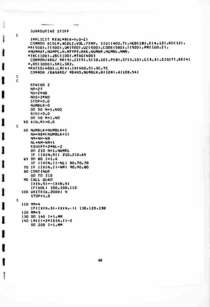
c c

SUBROUTINE STIFF

IMPLICIT REAL»8(A-HfO-Zl COMMON ACELRtACELZtVOLtTEMP, SIGI(400,7),HEOI It)tEIt«12),ROI12)«

*R ( 500) , Z ( 500), UR (500) tUZ ( 500) «CODE ( 500), T (500) t PRUGO ,2 I, *NUMMATtNUMPC,NvMTYPE,KKKfNUMNP«NUMELffNNN, *IBC(100),JBC(100),MTAGI400) COMMON/ARG/ RR(5),ZZI5)tSI 10,10),P(8)tST(3t10)tCI3t3)tSIGIT),EE(4) *,B0(1000),SRI,SR2, «RATI0i400),LM(4),lX(400,5),XC,YC COMMON /BANARG/ MBANOvNUMBLK,B(106),A(108,5«)

REWIND 2 NP = 27 N0»2*NB N02=2*NO STOP=0.0 NUMBLK«0 00 50 N=1,N02 B(N)=0.0 DO 50 M«1,N0

50 A(N,M)=0.0

60 NUMBLK«NUMBLK*l NH=NB*CNUMBLK*l) NM=NH-NB NL«NM-Nfl*l KSHlFT«2*NL-2 DO 210 N*1,NUMEL IF (IX(N,5)I 210,210,65

65 DO 80 I«l,4 IF (IX<N,I)-NL) 80,70,70

70 IF (lX(N,n-NM) 90,90,80 80 CONTINUE

GO TO 210 90 CALL QUAD

IX(N,5)«-IX(N,5) IF(VOL) 100,100,110

100 WRITE(6,2000) N ST0P«1.0

110 MM«4 IF(IX(N,3)-IX(N,» 1) 130,120,130

120 MM«3 130 00 140 1=1,MM 140 LM(I)*2*IX(N,I)-2

DO 200 1=1,MM

44

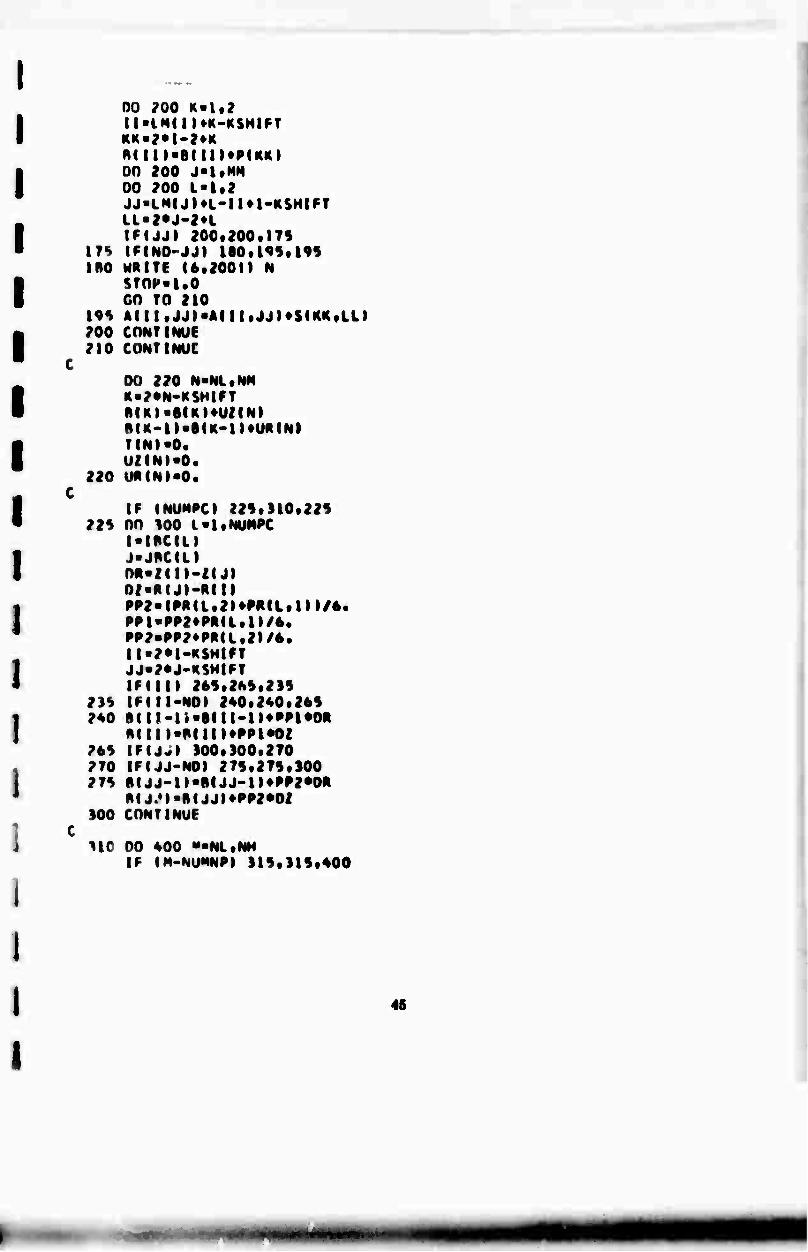
I I I

00 ?00 K-l,2 II-IM(IItK-KSHlFT KK«2»I-2»K Atlll«B(lll»PIKKI 00 200 J-ltMN 00 ?00 L-l,? JJ-LHIJML-1U1-KSHIFT LL«2«J-2*l IFUJI 200.200.ITS

I7S IffNO-JJI ie0.l<»S.l9S \no WRITE (6.20011 N

STOP-l.O GO TO 210

19S A(||.JJI*Ani.JJl*SUK.LLI 200 CONflNUE 210 CONTINUC

DÜ 220 N-NL.NM Ka2«N-KSH|FT A(K|.AlK|*ul(NI fl(K-ll-ftlK-ll*UitNI MNI-O. U2INI-0.

220 IH»IM»0.

IF (NUMPC) 224.I10.22S 22S 00 100 l«ltNUMPC

IMKIil J-JftCIU nR-/ni-/iji OI»RUI-RtII PP2MPRll.2MPRU.in/«. PPl>PP2»PRU.ll/6. PP2-PP2*PRU.2>/*. II-2»I-KSMIET JJ«2PJ-RSM|fT IMIII 26S.26S.2IS

2SS IPIII-*1DI 260.260.26S 260 A(n-Ii-B(ll-1MPP1*0R

RIIII-RIIII*PP1*0Z 76S IMJ^I S00.300.270 270 IMJJ-NOI 27S.27S.300 27S RIJJ-1I'(IIJJ-|I*PP2*0R

RIJ.,I«IIUJI»PP260I 300 CONTINUE

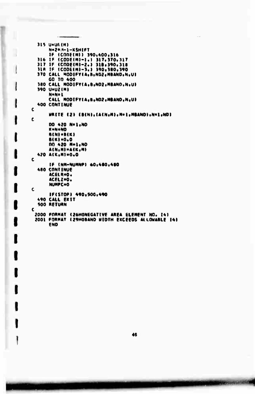
110 00 600 --Nl.NM If IM-NUMNPI 31S.31S.600

c

f

315 U»UMM) N»2*:i-1-KSHIFT IF ICOneCMII 390«400t3l6 If (COOEIMt-l.l 317V370«317 IF ICnOEtM|-2.| 318t)90t3l8 IF (COOE(M)-3.) 390,3i0.190 CALL MOOIFYlA,B.N02,»*8ANO,N.Ul CO TO 400 CALL MOD|FVUt6fND2fMftANO,N(Ul U«UI(M| N-NM CALL M00|FVU,B,ND2.NBAN0.N.UI CONTINUE

fSINIfUfNtNI»N«|tN6ANDItN«tf

00 420 N-I.NO «■N^NO 8INI«B|KI 8(KI»0«0 00 420 N«ltNO

1i

316 317 »I« 370

380 390

400

NRITE 121

420

480

NO I

AIN«NI*AIKVM| AIJC,«1-0.0

IF INN-NUNNPI CONTINUE ACEIR-O. ACELI-O. NUNPC-0

60t480t480

IFtSTOP I 490,900.490 «90 CALL EXIT 500 RETURN

2000 FORMAT (26H0NECATIVE AREA ELEMENT NO. 14) 2001 FORMAT (29H08AN0 MIOTN EXCEEOS AlL0UA8LE 141

ENO

46

SUBROUTINE OUAO

IMPLICIT REAL*SIA-HiO-n COHHON ACElRtACELZ «VOL t TEMP, SIGIUOO»7l t HEOl 181 »CUf 121 tROI 1211

•RI500»./(%00l,URI*0OI.U/|S00..fOü£(*.O0I.T|500»tPRIIC0t2lt •NUMMAT.NUMPCtNfMTVPEtKKKtNUMNPtNUNCLtNNNt • IBCt lOOItJBCIlOOIfMTACUOOl

COMMON/ARC/ RR(9lt22l9l»SltOtlOltPIBIvSTIl(10lfCllf9ltSIC(7lvEEI4l •tBOf10COItSRltSR?t •RATI0f400ltLMU|*|XU00t9l»XCtVC

COHMON /BANARC/ NBANOfNUMBLK»Bl10BItAClOBtB^I DIMENSION UUI.vm

CALL STRSTR nn DO JM.IO ÜÜ 120 I-I.3

120 STU.JI-G. on 130 i-itio

130 SII.JI-O. on uo IM** NPP>1X(N,II RRIII«RINPPI

1*0 Z/(M-/(NPP| xC>tRRII)*RRI2l*RR<3l«RRt*M/*« rf •!//( n»//l2IWZI3l»/ZI«M/4. RRISI-XC riifi«vc K»B JM I-* LMI3I-9 NT«* IffIXlNt3l-lX(Nt*ll 160*150*160

190 NT-I LNI3I-9 1*1 K-3 J«? XC*(RRni*RRf2l»RR|)ll/). VC«ll2ftl*llltl«ltCfll/S« MfflaMIH tt(fl«ftCII

160 On 200 UN-I,NT LMf 11«2*|-l IMJ2|.2*J-1 uin>/zf ji-zzui U(2)-ZZfKI-ZZfII •Jf 3I*ZMM-ZZUI

47

I

I vm>RR(K)-RRUI vm-pftm-RRU) Vl3l«RRUI-RRt II ARfA-IRRI Jl*U12l«RRMI*Ulll«RR<5l*U(lll/2. VOL-VOL^ARfA CONM-.75/ARFA XNT-NT COM-2#0/XNT COM-COM^COMM

00 180 L«lfl tl>lN|LI STCUIII-STIl.llinilLIKON SH?,IIMI-Sfl?.l!M»»VlL»»COH Sri3vIII«STI3(IIMV(LI«COM STM,||MI-Sfl3flUIUüUI*COK 00 ISO M«ltS JJ-LMIMI sttif jji«siiitJji»(uai*ciitii*uiNi«vtLiKiif3i*viMi«vaMCf itii^u HM|*UILI»Cll.JI»VIHn«CO»«N Slll«JJM)*SllltJJ*llMUll.)*Ctl*2)*VfM|*VlU*COf)l*UINt*V(ll*C(2t l3l«Vl«l*Ulll»ClltJI»ütMII»C0HM SI II»l.JJ»ll«Sni»l,JJ»llMVlL»»CI2»2l»¥l»<l»UUIK0.1l»Ul«l»üUI» lC(2t3l«VlM|»V(LI*Cf2t)t*UINn*C0NM S(JJ»ltlll*StlItJJ*ll

180 CONTINUE l-J J-JM

200 CONTINUE

tFllXtNv3l-IXfN9%ll 220f290»220 220 00 2*0 I«li2

KK-10-1 00 2*0 K«1VKK r.C-SlKK*l(KI/SIKK*|tKR»ll 00 230 J*lt3

230 STIJ,Kl-ST|J,m-CC»SHJ.K*MI 00 2*0 J-ltKK

2*0 SIJ.M-SIJfM-CC»SfJ.KK»ll 290 CONTINUE

ll«C IFINNN.EO.il GO TO 260 II ■*

260 SIGfll«-SICI(Ntll*ll*TEMP SIGf2l —SIGI(NtIU2l*TEMP S1GI3I—SIGIINttt«3l 00 920 I»It8

48

(M ll-C.O DO SIO J»l.3

510 P(l l«Pltl*STU*ll*SlGUl 520 ptn-pm«voL

nx»vnL»Ar.ELR»RO(MTVPEIM. 0Y-vril*Af.EU»RniHTVP6l/4. Of! 510 I«lt4 P(?»II-Pi?»Il*OV

530 P(2*l-ll-Pf2*1-II»DX RfTURN

49

SUBROUTINE STRSTR

IMPLICIT RtAL»8U-H,(W» COMMON ACELR«ACELI«VOLtTEMRf S!Gl UOOt 71 tHEOUS) f EUt 121 »ROI I2lt *RI9001.Z(9001•URI9001tUZt90011CODEISOOItTtSOOItPRIIOOf211 •NUMMAT.NUMPC.N.MTVRE.KRK,NUMNP,NUMtLfNNN. • IBC UOOI tJBCC 10011MTAGUOOI COMMON/ARC/ RR19)tZZ(9lfSllOflOI«P(Bl.STOflOlfCriflltSIGITIfEEUI

•RAT!OI400l.LM«4l,UI<»00.9I.RC,VC COMMON /BANARC/ MBAND.NUMBlR.BflOBI.Al 108.9*1

l-IXIN.n J«IX(N.2I MtXINfli L-IX(N,4l MTVPE*IX(N.9I VOL*0.

TFMP>nill«TUI»T(RI«TUII/4.0 00 90 XR-l.* EEUKI-E(KKtNTVPEI IFIMTACINIt 60.60.TO CC«ltttl#<tffflffll M«EEm/ll.-fcM2l"2l

cii.n*cnMM C(l.2l*CnMM*CC C(1.)I>0. ClttttKlltil C(2.2l-Cll.ll CI2.)I«0. cn.n-o. C()«2I«0. C(1.3)«.9*COMM*(l.-CCI CC-OTAN(EE161/97.2961 BB«DS0RTI9,0*12.0«CC*CC) EF(6I-CC/BB Efltl«l*8«tlfl/M CO TO 900

70 CC-0TANIEE(6|/97.296I RB*OS0RT(9.0*12.0*CC*CC) FEC6I-CC/BB EF(3l«3.*rE()l/BB CC«2.*(l.»EE(2ll/l9.-6«*EE(2n 0D«(SIGl(N.l)-SIGIIN.2ll/2. RJ2«(00*DD*SIG1(N.3I**2I/I1.-3.*IEE(6I**2I) BJ2«0S0R1(BJ2I

90

60

I

B.Jl>1.5*tSICI(N«l)*SIGIIN,?n-3.*tfeU)*BJ2 r)0*BJl/RJ2 BB«1.»9.*IEE(4I«*2I*CC Cr.-3.*FEUI«CC-DO/3. 00-tEm-00/6. Hl«.5«Cr./(BB*BJ2l H2-00«CC/BB-EEI2l«EEI3l/(BB*BJ2*;i.-2.*EE(2in H1-.5/(BB*BJ2*BJ2l

900

lt«Pflll/ll»Mflfll r.n.ll-RB»J l.-M?-2.«Ml»SICMN.ll-Hj»fSICHNtt»**2ll CU,7l--RB*(H2»Hl»(SIGIfN.n*SICIfN.2n*H3*SlGIIN»n*SICIIN*2ll Cl |,l)--RR*(Hl*SICIfN,ll«H)*SIGflN,l)*SlCMNv)l) Clttll«CCtttl CI2f2)-BB*ll.-H2-2.*Hl«SIGMN«2l-H3«(SIGIINf2l*#2ll C(?.))>-nR*(H|*SICIINv)UHl*StCIIN«2l*SPGIINv3ll citfii«cttfii ciftaiKittii CI1,1l-nn*f.5-H3*ISIGIfNt)l**2ll «FTURN END

! 51

SUBROUTINE HOOIFV(A«B«NE0tMBANOfN.UI IMPLICIT REAL*BIA-HtO-l| OIMfNSION All08t94l»BII08l 00 250 M-2.MBAN0 K«N-M*l IFIKI 215,235*230

230 H(KJ-B(K)-AfK,MI»U A(K,MI-0.0

235 K-N*M-l IMNEO-KI 250,240*240

240 HU»«BJK|-AIN,M»»U A(N*MI-0«0

250 CONTINUE AIN*1I«1.0 B(N)*U RETURN END

52

I I I I I

1

SUBROUTINE BANSOL IMPLICIT REAL*8U-Hfn-Z) COHMflN SRANARG/ MMVNUMBLK «BU08I» AliOSf 54)

NL-NN^l NH-NN^NN RFWINO 1 RFWINO 2 NB-0 GO TO 150

100 NR«NB*1 Ü0 1?5 N-ltNN NM«NN«N BCNI-BINM) B(NMI«0.0 00 125 M-l.MM AINtMI-AINMtM)

125 AINM«M)»0.0

IF INUMBLK-NB) 150.200tl50 150 READ (21 (B(NltlAINfM)»N>lvMM|vN«NLtNHl

IF (NBI 200tlC0t200

20C 00 300 NMtNN IF (AIN.II) 22^.100.225

225 B(NI»B(N)/A(N,1) 00 275 L-2.MN IF UIN.LII 230.275*230

2^0 r-A(N.LI/A(N.ll I«N»L-l JsO 00 250 K«l,NN J«JM

2S0 A(|fJ)-AIItJ|-C*A(N»K) B(I)>B( ll-A(N,ll*B(NI AIN.LI'C CONTINUE CONTINUE

275 100

i75

MOO

IF INUMBLK-NB» 375*400*375 WRITE (1) (B(N).(A(N*M)*M«2V CO TO 100

MM).N«I*NN)

00 t*bC M»ltNN N«NN*1-M 00 425 K-2tMN

63

I

I

7

1

NM«N«NN

ASO A(NM.NRI-HtNI NB>NH-1 IF (NBI <>79f500t479

«75 BACKSPACF I RFAO (1) IBIMtUCN.M|fH-2,MMI,N-l,NN» BACKSPACE 1 GO TO 400

c 500 K>0

UO 600 NH-lfNUMBLK DO 600 N-lfNN

NM«N«NN 600 B(K»-A|NM,NBI

C RETURN FND

SUHKOüTINC SfftESS IMPl KIT Bf Al •SIA-M.O-II f'IMMUN ACM M, ACM /.VOL. ff Ml-. SIGI (-0Ot M tHf OUSI tf Ut 1?) fKOUl I •

• w | SOOI t /f Scr. I vURI%00 11U/ I SOOI «Cmif I 50011 f 1400»tP«UCCt?11 • NU^MAf •NlfWPC»N««(TVP|(KKK«NUMNPtNUMFI ,HHH, •IHf • 10CI .JHCnCOl.Mf ACUOOI

f n^MUN/ABG/ *Rm./Zm«StlOtlOI.P(fll*SM)*10»fC(3»S)*SICmtEEI*) •tR0(1000l«SRl.SR?t •BAT|OI«.OCI.lM|4i»,l«l*OO.S,.KCtVC

CnNHON /BANARC/ MRANOtNUNRLRtSI|0*ttAl108tS%l

ini-o. SR-1. NUMR*0 HPRINT-O KKaO 00 300 N-l.NUMfl RATinfNI*!. IIINftMMMIIMlNffll MTVPE«IXIN|5I CALL OUAO NNM IM IHN, 1I-|XIN.«II l70tl6C.170

160 MN«) I7n nn IRO I»I.I

HR||l>0« nn IRO j-itHM

JJ"2*lXtN»JI 180 BRIII-RRf n»Sril.flMBIJJI»STf|,||-ll*Bf JJ-ll

00 190 1-1»! SIGIII-O. nn 190 j-it3

190 S!G(ll-SICIIMCIItJl*RR(Jl 00 195 |«tt1

19!> SIGHN.III-SIGIIN.IUStClli nn«ISIGIIN,5t-SIGIfN96f1/2. Aj?-IOl>»no»SIGHN.T»»»^l/ll.-J.*lfEI«l»»2ll AJ?«0S0RTfAJ2) AJ|>l.S*ISICilN,SI»SIGIIN(6ll-3.*CII«)*AJ2 PAti«AJt«ffC4l*Ai| IFIMTAGINI.EO.OI GO TO 200 IMNTACIM.FO.?! GO TO 100 nn-oARSiFAtL-eEnn CHECK*.02*EEf)) IFIOO-CHFCK) 300t300t196

196 KKX>1

CM<CHiCK/no IM(.H-SMI ivr.ioo.ioo

on m IOO ?00 CONTINMl

IFIMlL.LT.tFIlM CO fO ItO KKaKK^l no-ISIMINtll-SICMN.?!!/?, ^J?«JO()«nO«SICIlN.ll»»?l/II.-l.»IFfl*il«»?M nj2>OSOKTfllJ2l «Jl-l.S»ISICMN.ll»SICHN,7n-J,»eM«l»BJ? *AA«BJ?*BJ2 B6n»ftJ?*AJ? FFF*1.-3.*EEUI*FEUI CCC- ISICIINtll-SIGIIN.2ll*(SICIIN,S)-SICIfN(6IIM.«SlCIINt3l*SIGI

•IN.TI OOO-SICnNtlUSIGMN«?! CGr.-SIGIINt»l«StGlfNt6l FF-FFF*FFF GG*GGG«GGG UO*ODD*OOO CF»2.2**EEm*EEI4) AA>AAA*fF-EF*00 nR-BBB*FF-EF*GG CC*CCC*FFF-EF*000»GGG nn«i.)«EE(4i«EFn)*ooo FF-l.MEEf4»*EEm*GGG GG«EEI)I*EEI3I AAA*AA«BB-2.»CC BBR«AA-CC«00-FF CCC-2.*00-GG«AA GGG"BBB*BBB-AAA«CCC GGG-OSORT(GGGI IFfAAAl 220t210t220

210 RAT|0(N)«.9*CCC/BBB GO TO 300

220 AA-RBB/AAA BB«OARSfGGC/AAAI RATiniNI-AA-RB IFfRATlniNI.LT.O.I RAT|0fNl«AA^RR IFIRAnniNI.GE.l.l RAT 101VI-.99999 IFfRATIOfNI.LT.O.I RATIOfN)«0.

300 rONT!NUF

IFtKK.EQ.OI GO TO 420 00 3)0 N-ltNUMEL IFfMTAGCNI.GT.OI GO TO 350 nO-RATIOIN)

56

|F|UI)-SRI 305t350«)50 ^OS SR»Oü

KKK'l *so coNfmui

IflSH.lT.O.l» SR-O.l IFINUM^.FQ.OI GO TO «20

C ?60 DO 370 N«l,NUMEl

IF(MTAGCNI.CT.O) GO TO 370 IMRATiniNI.LE.SR) GO TO 355 no>RATin(NI-SR IF(00-.05| 355*355*370

355 MTACINtM 370 CONTINUE

r ^70 CONTINUE

00 «10 N>.*NUMNP !I«2*N-l R( I Il-R( m*SR

410 Ft! ll»l»»R( IU1I*SR DO 600 N>1*NUMEL i-ix(N*n J»IX(N*?) MtXlNttl L>IX(N*4I MTVPE.IX<N*5I IF(K.EO.L) GO TO 460 XC>(Rm*R(J)*R(K)*R(L))/4. VC*IZ(II»ZCJ>*Z(K)*Za)»/4. GO TO 4 70

460 XCs(RiII«-R(J)»R(K||/3. YC«(Z(n«Z(JUZlKII/3.

470 CONTINUE 00 450 I =»1*3 11»1*4 SIG( n«s(Gi(N*m-siGi(N*n SIGI(N*m«SIGm*U.-SR) SIGI(N*III«-SIGI(N«in SIGI ll«Slfil n»SR*SIGMN*II

4so siGicM,n»siG(n SIG(7I>FF(2)*(SIG(1I«-SIG(2M DO 455 1x1,4

^55 fcH Il = t(I*WTVPEl IF(MTAG(NI.EO.O) GO TO 500 CC = DTAMEEm/57.296» BB*DSÖRT19.0*12.0*CC*CCI FF(4)=CC/BB

57

I I I I I I I I I I 1 I I I I I I

nn-isiGlDTSiGmi/?. nj2<>(nO*no«SIGm«*2l/U.-3.f(fEUI**2ll

MM n*.s*m(.m«sM.m»- ».mm^Rj«' soo si(.i(N,^i«si(.(n

CC«(SICIll«StO<2M/i« Rn*(SIG41)-Sir.(2t |/2. CR>0S0RT(RB**2^SIGC3)**2) SI6(4)*CC4>€R SIG(5)«CC-CR SIG(6}«0.0 IF ((BB.F0.0.0).AND.(SIG(3).EQ.0.0II GO TO 510 SIG<6)»28,698«0ATAN2(SIG(3)tBB|

510 CONTINUE IFIHPRINTI 520,520t550

520 WRITE(6,20001 NNN MPRINTx50

550 MPRINT=MPRINT-l WRITE (6» 2001» N.XCtVCttSIGnif I'ltTltMTAGfNI lF(MTAG(N).EQ.O) GO TO 560 D0-(SIGI(Nt5l-SlGI(Nt6ll/2. RJ2»<OD*DO*SlGl(N,7l«*2)/(l.-3.*IEEU>*»2n RJ2«OSQRT(BJ2} TnL=TOL*BJ2 GO TO 600

560 SIGm*EE(2)*(SIGMNv5)*S!GI(Nf6M BJ2« OSQRTCtCSIGl(N.5l-SlGI<Nt6l)**2*ISIGICN,6l-SIGI7ll**2*«SIGIT> *-SICI(N.5l)*»2»/6.0*SIGnN,7)**2l T0L*T0L*BJ2

600 CONTINUE SR2= (SRl*SRI 4- SR2 SRI* (l.O-SRI ♦ SRI WRITE(6(2C02) TOL.SR •NUMRtKKtSR2 IFfTOL-l.l 660,660t650

650 KKK=I GO TO 700

660 KKK»0 700 CONTINUE

11=0 00 710 IMtNUMEL

710 IFIMTAGIU.GE.ll II'IIM IFIKK.GE.NUMELI CALL EXIT

800 RETURN C

2000 FORMAT!1H1/ ♦36H STRESSES AFTER APPROXIMATION NUMBER 14//// ♦7H EL.NO. 7X IHX 7X IHY 4X 8HX-SIRESS 4X 8HY-STRESS 3X 9MXV-STReSS ♦ 2X 10HMAX-STRESS 2X 10HMIN-STRESS 7H ANGLE 4X BH2-STRESS 5X 7HPL

♦ASTICl 2C01 FORMAT ( I 712F8. 2« IP5F12.4 tOP lf7 . 2«IPEW.^t 1121 2C02 f-QRMAT(^9H0THE UNBALANCED LOAD Af THIS STAGE IS EU.5//

♦47H THP RATIO FOR CORRECTION OF STORED STRESSES IS FIG.4// ♦31H THE NEXT ELEMENT YIELDING IS U/ ♦91H AND THE TOTAL NUMBER OF ELEMENTS THAT CAN YIELD WITH THE LINEA *P ADDITION OF TOTAL LOAD IS 14/ ♦50M LOAD UP TO THIS STAGE AS A FRACTION OF TOTAL IS F20.5 »

END

I

I I I i

59

I

I I I I I I I I I I I I I I I I

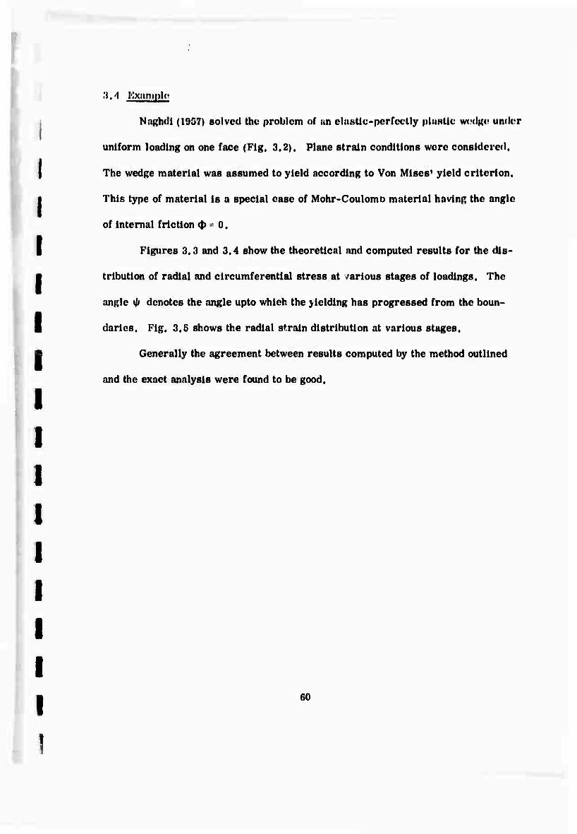
3.4 Kxiimpl«'

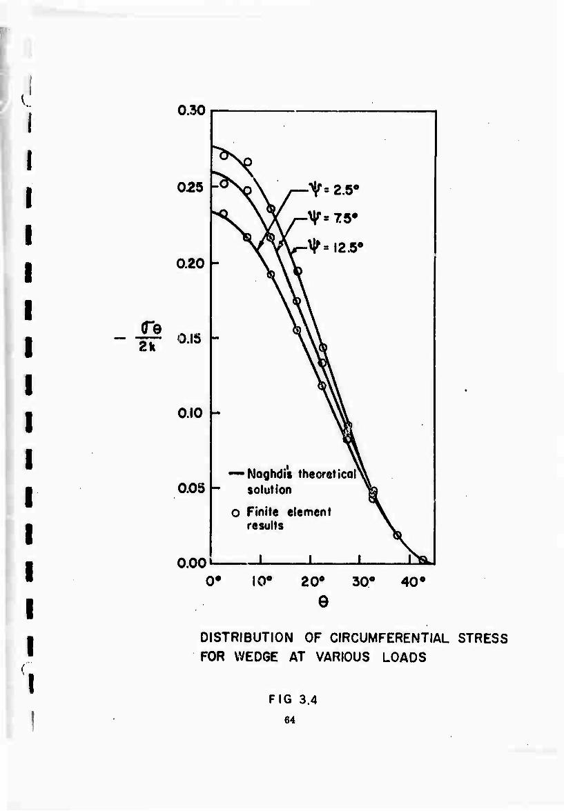
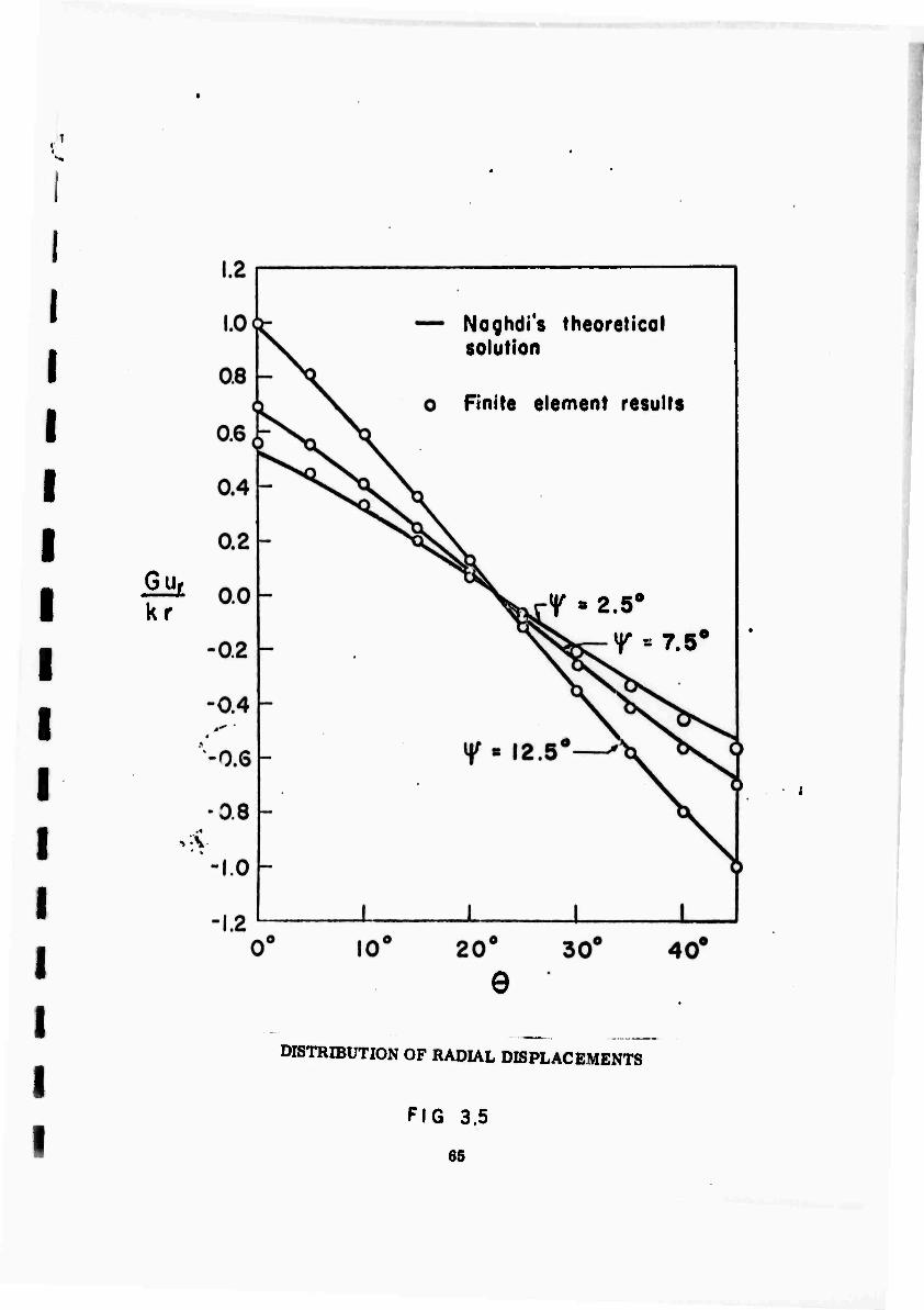
NiiKhdi (19S7) solved the problem of an elaHtiu-pcrfcctly plaHlic wodHO UIKUT

uniform loading on one face (Fig. 3.2). Plane strain conditions were considered.

The wedge material was assumed to yield according to Von Mises' yield criterion.

This type of material is a special case of Mohr-Coulomo material having the angle

of internal friction <t> 0.

Figures 3.3 and 3.4 show the theoretical and computed results for the dis-

tribution of radial and circumferential stress at various stages of loadings. The

angle i/» denotes the angle upto which the yielding has progressed from the boun-

daries. Fig. 3.5 shows the radial strain distribution at various stages.

Generally the agreement between results computed by the method outlined

and the exact analysis were found to be good.

60

CALCULATION OF STRESS RATIO

FIG 3.1

fil

W lb/in

FINITE ELEMENT IDEALIZATION FOR ELASTIC-PLASTIC WEDGE

FIG 3.2

62

0.8

I I

2k

0.6 h

0.4 h

0.2 h

0.0 h

0.2

-0.4 h-

-0.6

-0.8 h-

-1.0 0« 10'

—-Naghdis theoretical solution

o Finite element results

20* 30* 40^

DISTRIBUTION OF RADIAL STRESS FOR WEDGE AT VARIOUS LOADS

FIG 3.3

63

c

(Te 2k

025 -Ö>^\ -V3 2.5*

0.20 v\ 1

f-^=l2.50

0.15 -

\

0.10 -

\

0.05 — Noghdis

solution thecreticaPÄ

O Finite element ^k results \

nnn 1 1 1 PSL

10* 20°

e 30° 40*

DISTRIBUTION OF CIRCUMFERENTIAL STRESS FOR WEDGE AT VARIOUS LOADS

FIG 3.4 64

Gu, kr

Naghdi's theoretical solution

Finite element results

f » 2.5° r = 7.5°

DISTRIBUTION OF RADIAL DISPLACEMENTS

FIG 3.5

65

I

CHAPTER IV

COMPUTER PROGRAM FOR ANALYSIS OF JOINTED ROCK

rhaplor IV. Coiniuilrr l>rtit;r:ini Foi AnnlyHlH ol JolnltMi Koik

4.1 OrKanty.atton

The computer program described htfl Is based on the theory described In

Chapter I and II. The rock mass is considered as a linear elastic material in the

direction of compressive stresses and is assumed to have no resistance to defor-

mation in the direction of principal stresses. The program corrects the discrep-

ancy in the method presented by Zienkiewicz et al (1968). This was pointed out

towards the end of Chapter I. It makes allowance fur the boundary conditions,

residual stresses, stresses due to temperature change, and varying pressure

boundaries. This program also us« A the quadrilateral elements and generates

stiffness the same way as that described in Chapter III.

The principal program called MAIN controls all the data input and control

information. It does the system initialization, prints the control data, geometrical

and material properties. MAIN calls the subroutines for stiffness, solution of

equations and stress calculations.

4.12. Stiffness Matrix

Stiffness matrix for the analysis is computed in blocks by the subroutine

STIFF. For element stiffness, it calls QUAD for triangular and quadrilateral

elements and ONED for bar elements. Direct stiffness technique was used to get

the total stiffness. Equations are modified for displacement boundary conditions.

I

I

I

(

I

I

4.13. Load Matrix

Load matrix for the analysis is computed in LOAD subroutine. The varying

pressure boundary is taken into account. The load matrix is modified in the LOAD

subroutine for each iteration performed. This accounts for the nonlinearity intro-

duced by progressive cracking by considering the change in element stiffness as a

pseudo load.

4.14. Calculations of Displacements

After the stiffness and load matrices for a stage have been computed, the

resulting equations are solved by calling subroutine SYMBAN. This subroutine

was developed to take the advantage of the fact that stiffness matrix remains the

same throughout. Gaussian elimination technique is used to solve the equations.

The elimination is done once for all and the reduced matrix stored on auxiliary

units. Solution for each iteration consists of back-substitution only. This approach

results in considerable economy in machine time.

4.15. Calculations of Stresses

After the displacements have been computed, the stresses are computed

using the constitutive law. A change in the minor principal stress corresponding

to Poisson's effect has been introduced when one of the principal stresses was

compressive and others tensile.

67

4.2. Input Data Preparation

1. Control Card (A6). This card will carry the characters START in columns

1-5. This will start the processing of the data deck which consists of the

following set of cards.

2. Job Title (72H). This card will give the descriptive ider tification for the job.

3. Control Information (415, 3F10.2, 15, E15.4)

Information Columns

Total number of nodal points 1-5

Total number of elements 6-10

Number of different materials 11-15

Numl»or of pronHiire houmhiry ciircls Hi - 20

Body Force in X-direction 21-30

Body Force in Y-direction 31 - 40

Reference (stress-free) temperature 41 - 50

Number of Iterations 51 - 55

Tolerance to Convergence 56 - 70

4. Material Property Cards. One set of cards must be provided for each material.

In each set:

a. First card (215, F10.3, 15) will give the following information:

Material identification number 1-5

Number of temperature cards (8 maximum) 6-10

Mass density of the material 11 - 20

68

Material code to designate materials 21-20 which cannot take tension

code = 1 for materials which cannot take tension 0 for materials which can take tension.

b. Subsequent cards, one for each temperature, the number being

defined in columns 6-10 of the first card, will carry the following infor-

mation (4F10.0):

Information Columns

Temperature 1-10

Elastic modulus 11-20

Poisson's ratio 21 - 30

Coefficient of thermal expansion 31 - 40

5. Nodal Point Cards (K, F5.0, 5F10.0)

One card for each nodal point with the following information:

Nodal point number 1-5

Type of nodal point 6-10

X-ordinate 11-20

Y-ordinate 21-30

XR 31 - 40

XZ 41 - 50

Temperature 51-60

If the number in columns 6-10 is

Zero XR is the specified X-load and XZ is the specified Y-load

1 XR is the specified X-displacement and XZ is the specified Y-load

69

•

I I

2 XR is the specified X-load and XZ is the specified Y-displacement

3 XR is the specified X-displacement and XZ is the specified Y-displacement

All loads are considered to be total forces acting on an element of unit thickness.

Nodal point cards must be in numerical sequence. If cards are omittod, the

omitted nodal points are generated at equal Intervals along a straight line between

the defined nodal points. The necessary temperatures are determined by linear

interpolation. The type of the nodal point, as well as XR, XZ, are set equal to

zero.

6. Element Material Cards (1215)

These cards shall carry the material type of all the elements. Each card

shall have material types for 12 elements in sequence. The material type

for each element must be read in as no Interpolation has been provided for.

7. Element Cards (515, 5X, 3 F10.0)

One card for each element will provide the following data.

Information Columns

Number of clement 1 - 5

Nodal point I 6-10

Nodal point J 11-15

Nodal point K 16-20

Nodal point L 21-25

Initial stresses: (I) component In x-dlrectlon 31-40

(li) component In y-directlon 41 - 50 (iii) shearing stress on x-y planes 51-60

70

Nodal points ItJ,K,L are comers of each individual element in a counter-

clockwise order for a right handed system of coordinates. For triangular

elements set nodal point L same as nodal point K. The element cards

must be In the numerical sequence. Any cards that are omitted will be

automatically generated in the program by incrementing each of the I, J,

K, and L nodal points by one.

8. Pressure Boundary Cards (215, F10.0)

One card for each boundary element which is subjected to a normal

pressure will carry the following information:

Information Columns

Nodal Point I 1-5

Nodal Point J 6-10

Normal Pressure at I 11 - 20

Normal Pressure at J , 21-30

As shown in the sketch, the boundary element must be on the left as one

progresses from I to J. Surface tensile force is input as a negative pressure.

Output Information:

The following information is developed and printed by the program:

1. Reprint of input data

2. Nodal point displacements

3. Stresses at the center of each element

71

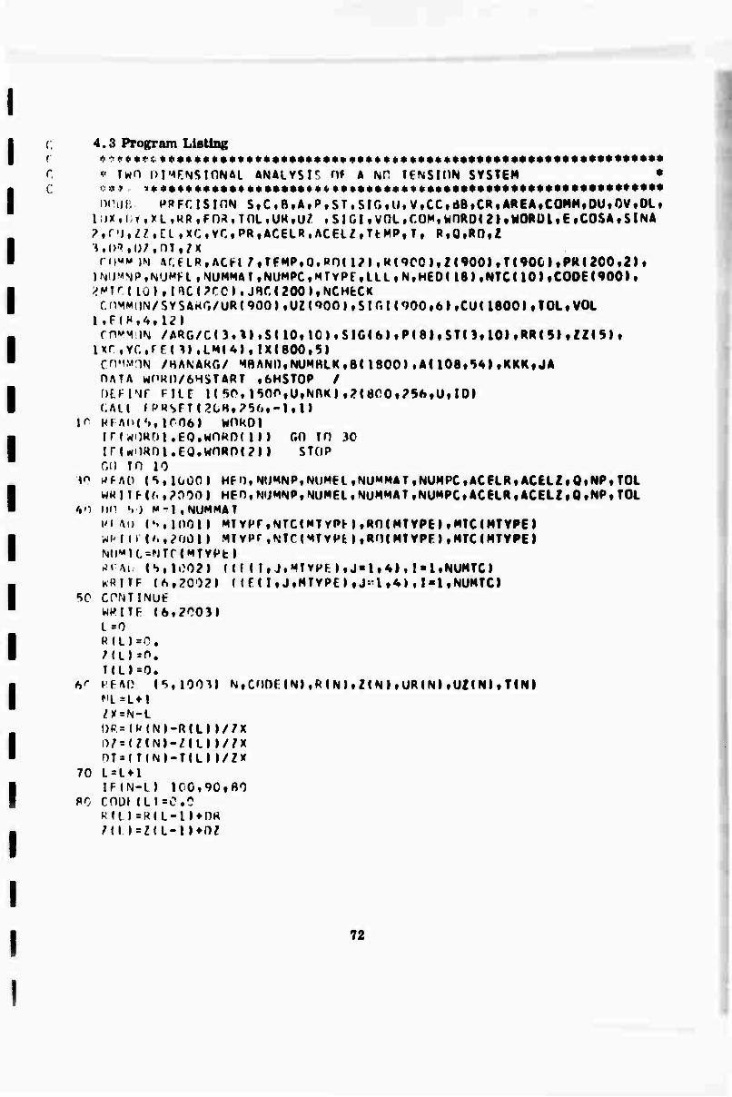
(. 4.3 Program Listing r * •**«*!!•■:. ************************** ****••*•«•«*«*****•********•***** r <■ TrtO lUM^NSlON&l ANftLVSIr Of A Ml TENSION SYSTEM ♦ c ••* •. ««♦♦»»•♦♦»♦♦♦♦♦♦♦»♦»«.♦•♦♦»♦»♦♦•«.»♦»»»••»»♦•••♦♦•♦♦♦••♦♦•♦•♦*

DOUB PP FC IS IHN S,C,B,A,P,ST,Sir,,il,V,CC,cJBtCRtAREAfCOMM,OUiOVfOLf 1 )X,| r.XL.KRtFn^.TnLtUM.U/ iSlCItVOL.COMtMnROlZUMORUlvEtCOSAtSlNA ?,('), U ftl .XC.YCfPRtACELRfACF.LZ|T^MPf T, R,0,ROtZ l,l)->,l);f nT.M

r.riMUJN ftr.KRf ACH 7tTFMPt0.Rn(m ,R(<)C0ttZ(900ltT190CltPR(200f2)f IN I-'VJP.N'JMH .NUMMAl .NlIMPC.MTrPf »III »N.HEO« 18 t »NTCMO I f CODE (90011 2P?r UOI • I ACI?C0I t JHCItOOIf NCMfcCK

( nvw )N/SYSAKi;/uR(900l,UZ(f»00>,Sir.I('>00»6l,Cun800lflOLfVOL 1 ,F(H,/*t 12|

rnMM )N /ARG/C(3.1l(S(l0«10)tSIG(AltP(8ltSTn«10lfRRI5ltZZ($li ixr.vcrrc \»,LH(4J, ix(800i5»

CnMMJTN /HANAKG/ MHANI),NUMBLK , BU 800 I . Af lOStS^I ,KKK , JA OATA Wf'KIV6HSTART ,6HSTüP / DtFINF FHC M «iO.lSOO.UtNnK» ,?1800f?56tUtlOI (AU f PXSrTI^CH, ?56t-!ill

K RFAI)(%f IfOAl WdkOl irrw')Rrji.60.wo«n( i)» on TO 30 iruimm.EQ.wnRom) STUP mi in 10

40 JI-AP (S.lOGni HFn.NUMNPtNlJMEl.NUMMATvNUMPCtACELRtACELZtOtNPtTOL WHITF(^f?nOO) HFn,NiJMNPtNUMELfNUHMAT,NUMPCtACELRtACELZtQtNPtTOL

/♦o DP sj M-l »NUMMAT l'l AD ('.,10011 MTVPF.NTCIMTYPI-ItRniMTVPEI .HTC1MTVPEI WRIII ('.,?i)01) MTYPrfNTr(^TYPt),Rfl|MTVPF»,MTC(HTVPEI Nl)«1C=NTr(MTYPt I -'Ai (S,100?l I (M I,J.«TVPF.l,J«l,4l,I»liNUMTCI NRITf (ft,?0')?l ( (FlitJfMTYPEItJ-!lf4»tI«l.NUMTCI

SC CPNTINUF WPITF (6f?C03J 1=0 R(ll»0. ML»=0. T(L)=0.

6^ h'FM? (S.IOOIJ N,CnnF.(NI,RINIfZ(NltUR(NlfUZINItTINI f|L=L*l ZX = N-L DR«(R(N)-R(tlI//X l>/«(Z(N)-ZU} »//X nT=(T(NI-T{Ll»/ZX

70 L=L*1 IF(N-l) lC0,9G,fl0

pc cno\ (L»=c.': Rlt)»R(L-l}^OR MU = Z(L-mr)z

72

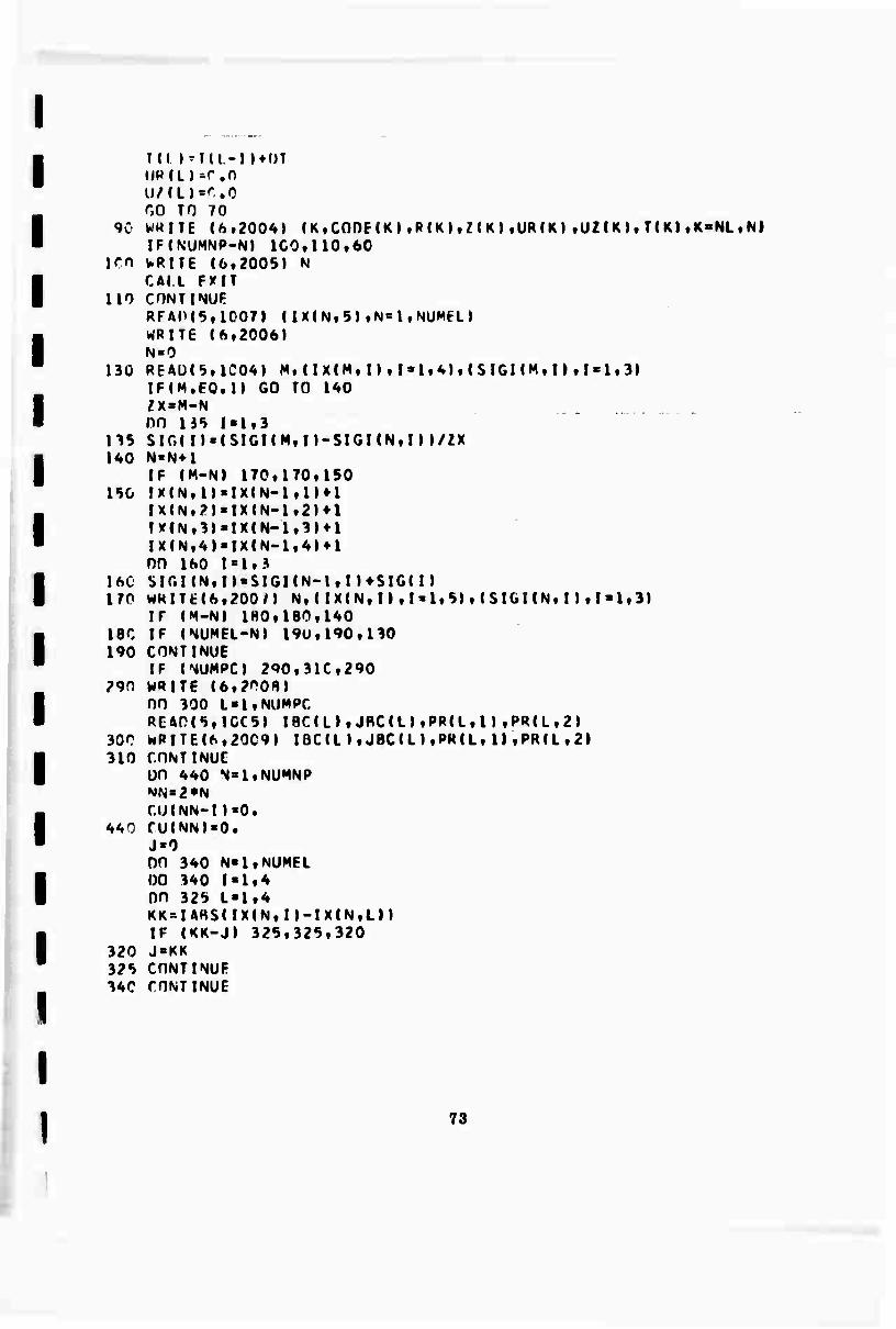
T(l IMll-l »♦OT

GO TO 70 90 WHITE (6.20(H) (KtCnnE(K)«R(K)vZ(K),UR(K)«UZlKI«TIK)tK>NLtNI

IF(NUMNP-N) lC0ill0t60 KO WRITE (6f20O5) N

CÄIL FXIT 110 CHNTINUE

RFAIM 5, 1007) (IX(Nt5)tN-I *NUHEL) WRITE (f>f2006) N = 0

13ü RE4Ü(5*1C0^) M*(IXIM(I)«I>1^)»(SIGI(M,II tl<l,3l IF(M.EO.l) GO TO 140 2X=M-N DD US I»l,3

US SIG( I) = {SIGnM,n-SIGI(N.I))/2X HO N*NM

IF (M-NI I70fl70tl50 ISO I*(N,l)«mN-ltl)*l

IXIN,?)«IX(N-lf2)*l !»(N,3»»IXIN-li3)*l IX(Nf4)-IX(N-lt4)4-l nn ibo i=i,3

160 SIGI(N»I)>S1GI(N-1VIUSIG(I I 170 WHITb(ft,?00/l N»(lXlN,n,I»l,5)»(SIGMN»ll*I»lf3l

IF <M-N| 180»180,U0 18C IF (NUMEL-NI 190,190,130 190 CONTINUE

IF (NUMPC) 290,310,290 290 WRITE (6,2008)

00 300 L»1,NUMPC RCarCi.lCCS) IBC(L),JRC(L),PR<L,l) ,PR(L,2)

300 WRITE(6,20C9) IBC(L),JBC(LI,PH(L,1),PR(L•2» 310 CONTINUE

OH <*<*0 N=1,NUMNP NN=2*N CU(NN-I)«0.

^AO fUlNNI«0. J«0 DO 340 N»l,NUMEL DO 340 I«I,4 DO 325 L«l,4 KK = UnS(IX(N,I)-IX(N,Ln IF (KK-J) 325,325,320

320 J=KK 325 CONTINUE 340 OONTINUE

73

I

WR1 TF(ftt?012» MH^^|0 ASO CAI L SMFF

NCMECK«! KKK = l rail SYMRAN KKK = 2 nn «soo iLL = lfNP CALL LOAD CAJ L SYMftAN Oil ^00 N = 1,NUMNP MN = 2*N ClHNN-1 )=CU(NN-l)*B(NN-n

400 CU(N^»=CU(NN»*B(NN» WRIT6(^»2013I LLL WRITE(6,20lO) (N,B(?*N-n«B(2*NI*CU(2*N-l)fCU(2*Ntt N ■ ItNUMNP) CALL STRFSS IF{MCHECK,FO.O» GO TO 600

SOO CONTINUF r,() T) 700

600 WRITfc(6,20ll) Lll 7GG CO TO 10 999 hORMAT(IS) ICCC FORMAT n8A4/4I5f 3Fl0.2f I5,E15.A, 15» inn FORMAT (2I5,IF10.3,I5» 1002 FOttM^T ««JFIO.S) 1001 FORMAT (I5,F5.1,5F10.4) IOC* FORMAT ^I5,5X,3F10.4» 1005 FnRMAT(2I5,2F10.3) 1C06 F0RMAT(A6) 1007 FORMAT!12151 20C0 FORMAT (IHl 18A4/

1 30H0 NUMBER OF NODAL POINTS 13 / 2 30H0 NUMBER OF ELEMENTS 13 / 3 30H3 NUMBER OF OIFF. MATERIALS 13 / '* 10H0 NUMBER OF PRESSURE CARDS 13 / 5 30H0 X-ACCELERATION E12.4/ 6 IDHO Y-ACCELERATION E12.4/ 7 30HÜ REFERENCE TEMPERATURE F12.4/ R 30H0 NO. OF APPROXIMATIONS 15/ 9 30H0 TOLERANCE FOR CONVERGENCE E12.4)

2001 FORMAT t17H0MATEMIAL NUMBER» I3t 30H, NUMBER OF TEMPERATURE CARDS» I II, 15H, MASS DrNSITY= El2.4tl6H, MATERIAL CODE» 15»

2002 FORMAT (15H0 TFMPERATURE 10X 5HEC 9X 6HNU 10X 5HALPHA/ I(Flb.2,3EI5.5l)

2003 FORMAT ( lOBHlNOOAL POINT TYPE X ORDINATE Y ORDINATE X LO IAO TR OISPLACfcMFNT Y LOAD OR DISPLACEMENT TEMPERATURE >

?CC4 FORMAT (I l2.Fl2.^,2F12.5,2E24.7fFl2.3»

74

20))^ Uli'MAT (^6H0NniJAL PflINT f.AHL) tKHOK N- 15 1 inoij FOH^AT CWHlFLtMFNT NO. I J K L MATfRIAL

1SICIXX SIGIYV SIG1XY I 20C7 J-OHM&T mi3fM6,lIl2f3Fl2.3l 2008 FDRMAKPQHOPRESSURF BOUNDARY CONDIT lONS/^OH I J PRESSUR

l^ I PRESSURf J» 2009 Fi)HMAT(2I6,2FU.3) 2010 rrrr^ATl 12H0N.P.NUMBER 17X 3Hl)UX 17X 3HDUY 18X 2HUX 18X 2HUV/

1(IU2,^F?0.7J ) 2CII FORMAinSHO NUMBFR OF CYCLES TO CONVERGENCE = 151 2012 rnRMAT(?BH BAND WIDTH FOR THIS DATA = 15» 2C13 FnRMAT(30Hl RESULTS OF ITERATION NO.- I5///I

FNU

75

■' .vmmmimmmammmmmmmri -

SURRUUTINF STIFF

nnURLE PRECISION S,C.B.A,PtSl,SIG,U.V,CC,B8,CRtAREAfC0«MtDU»0Vt0Lt inx,OY,XL,PH,FORfTnL.UR,UZ ,Slbl»VOL.COM,EtCOSAtSINA ?fCU,ZZ,FF,XC.YC,PR,ACELR,ACFLZ,TfcMP,Tf R,a»KOTZ COMMON ACELR, ACFL Z,TEMP,0.RO( 12 ) ^("9001,2(900 It T(900 I tPR<200t2 It INUMNPfNUMELfNIJMMATfNUMPCfMTYPf ,LLL»NfHEO(l8l fNTCf 101,CODE(9001 t 2MTC( 10) , IBC(200).JBCI2001,NCHECK CHMMnN/SYSARG/llR( 900 )fUZ( 9001 fSIG 1(900,6 I fCU( 18001 tTOLf VOL 1,5(8,4,12) COMMON /ARG/C(3,3),S(10,IOI,SIG(6I,P(8I,STO,10I,RR(5I,ZZ(5I, 1XC,YC,FE(3l,LM(4),IX(800f5l COMMON /BANARG/ MBANO,NUMBLK,B(1800 I,A( 108,541»KKK,JA 0FF1NE FILE 1(50,1500,Ü,NBKI,2(800,256,U,101 NB = 27 ND=2*NB ND2=2*ND STOP=0.0 MUMBLK=0 JA = N02*( M8AN0M ) /1500M NBK=l DO 50 N=l,ND2 DO 50 M=l,ND

50 A(N,M)=C.O 60 NUMBLK=NUMRLK+1

NH=NB*(NUMBLK+l) NM = NH-NB . _ . NL = NM-NBM KSHIFT=2*NL-2 DO 210 N=l,NUMEL IF (IX(N,5)) 210,210,65

6S DO ftp 1=1,4 IF (IX(N,I)-NL) 80,70,70

70 IF (IX(N,I)-NM) 90,90,80 80 CONTINUE

GO TO 210 90 IF(IX(N,3)-IX(N,2)) 95,85,95 85 CALL ONED

IX(N,5I=-IX(N,5I MM = 2 GO TO 130

95 CALL QUAD IX(N,5)=-IX(N,5) ID = N WRITF(2MD) ((C( IIKtJJK),JJK=l,3l,EE(IIKl ,IIK»1,3I

1 ,((S(JJI,KKI),KKI=l,8),JJI=l,e),((ST(|KK,JKKI,JKK»l,8l,lKK»l,3l 2 ,(RR(JII),ZZ( JIII,JIIsl,4l,XC,YC,TEHP,V0L IF(VnL) 1^0,100,110

76

ico wkiTr(ftt?onoj N 5Tnp«i.o

11^ »v-t* 1 F < I < ( v , 1) - I X ( N,'. M 13011 2C, I 30

120 MM=3 130 DO UO l=ltM^ UO L^( 1)=2*IX(N,I »-2

DD 200 I»1,M«< On 200 K»lt2 Il=LM(I)*K-KSHIFT KK=2*I-2*K DO 200 J'l.HM DO 200 L«lf2 JJ=LM(J)*L-II*l-KSMIFT IL=2«J-?*L IF(JJ) 200f200,175

175 IFIND-JJI |ft09lfSfl9f IRC WRITE (6,20011 N

STnP»l.O GO TO 210

19S A(II,JJ)=A( n,JJ)*S(KK,LU 200 CONTINUE 210 CONTINUF

DO <»)C M = NLtNH IF (>1-NUMNP) 315,3l5f^00

3l,> U=UK(M) ^=2*M-1-KSHIFT IFCC10E(M)| 3yCf^00,3l6

Mft IKC'IDECM»-!,» 317,370.317 317 IF(r.ll)F(M»-c.l 31B,3<»C.31B 31« irCC')l)e(M)-3.» 390,380.390 370 CALL yODIFY(A.Nn2.M8AND.N|

GO TO 400 380 CALL ^nnirvu»Nn2.MBAN0.N» 390 U«UZ(M)

N=NM CALl MP0IFV<A.Nn2.MBAN0.NI

400 CONTINUE WKITFIMNBK) IIMN,MI,M«l,MHANOI ,N»l.NOI mK'mK*jt( nn 420 N«I.NO

K=N*MO 00 420 M»1.ND A(N,MI>AIK.M)

420 A(K,M)=0,0 IKN»1.LT.N0MNP» GO TO 60 nn 4*0 NM.NUMU IX(N,r>) = IABS(lX<N,5M

77

<.P0 CUNT INDf iF(STnpi <»<»Ci^crf*9c

AO.. (AIL f*IT riOO PfTURN

?rCC FdRMM (?6H0NEGATIVF AREA fLtMCNT NO. 141 2001 fOKMAT (?QHUHANÜ WIDTH EXCEEDS ALtUWAULE 141

FND

78

I

VIMW'NJl I NP (INI IJ

DOURLE PRKCISION S.CtO»A,PfST,SIGfU,VtCC,flB,CRtAREAtCOMM,DUfDVtOLt nix,i)Y,xL,Pf<,Fim,ini,uRiü/ ,sici,voL»cnMft,COSA,SINA ?,r.U,ZZ,EF,Xr,fYC.PRiACFLP. tACELZtTEMPtT, R,Q.ROiZ

CnWHON ACELRtACEL7.TEMP,Q,RO(l2».Pl9O0lfZl900I.TI900I.PRf200.2l* lNUMNPtNÜMELtNUMMATtNUMPCtMTYPEfLLL»NtHEO(L8),NTC(10»tC00E(900l♦ ?MTC(lO),IRC(2üOlfJBC(200).NCHECK r.0MMQN/SYSARG/UR«900ltUZ»9O0)tSlGn900i6l,CU(l800)»TOL.VOL

COMMON /ARG/COt 3t«SllOf 10)f SlG(6)«P(8)f STOtlO) ,RR(5»fZZ(5l • lXCtYC«EF(3)fLM(4)tIX(800t3)

COMMON /BANARG/ MBANO,NUMBLK.BC1800»»Ai108,54»,KKK,JA

JDO 100 1=1,8 P(11=0.0 no nc j*i,8

■ ioc s(i,j)=o.o I

c c

MTYPE=1X(N,5) i = ix(N,n J'IX(N,2) DX»R(J)-R(I» nY=z(j»-zm XL=DSQRTiOX**2*OY**2» CPSA»OX/XL SINA«OY/XL CHMMaEIl,2,MTYPE)*Ell,4,MTYPEI/XL

S(I,I»»C0SA*C0SA*C0MM S( l,2)=CnSA*SINA*CGMM S(l,3)»-S(l,l) S<1,4)—S(l.2l S(2,n>S(l,2) S<2,2»=SINA*SINA*C0MM SUtS)**S(lf2) S(2,4»=-S(2,2) SO«U«i«(|tl) S(3,?I=S(2,3» S( *, M = sn,i)

s(4,n»s(i,A) SU»2)«S(t*4) S(4,3»=S(3,4I SU,4) = S(2,2)

RETURN

79

SimwillT INE OUAI» noijRLE PRFCISION S» C t B t A * P * ST t S IG t Ut V tCC * BBtCK t AREA «COMHt OUf OV tOL »

ll)Xfr.Y,XL ,RKfF(iMf TflLtURtU? , S !GI , VOL .COM, f ,COSAfS INA ?,CU,/Ztrr ,xC,YC,nR,ACELR,ACfcLZfTEMPfT, R.O.ROtZ 3,UfV.XT,XS.RATinfnENtXNT

CnMMON ACtLR,ACELZ,TEMP,g,RÜ(l?l,Ri900)»Z(900)fT(90C»tPR(200t2)t INIJMNP,NIJMEI ,NUf"^ATfNUMPC,MTVPFtLLL,N|HE0ll8»iNTCt 1011CODEC 900» . ?^TC( 10),lRC(2rCI,JBCI200»,NCHECK Cf)MMilN/SYSARG/UR(900) »UZ ( 900 ) , SIGI (900 »6 ) |CU( 18001 tTOLtVOL

l»fti»4tlil COMMON /ARG/C<3,3)«S(lOt10)*SIG(6I,P(6ttSTf3,10)*RRI51,ZZ(5 It

lxr,YCfFF(3)fLM(A),IX(800,5) COMMON /BANARG/ ^RANO.NUMBLK.Ot1800JtAC108f54»»KKKtJA

niMFNSIDN U(3).V(3) l = IX(N,n J=IX(Nf2) K=IX(N,3) L=IX(N,4) vrYPE=IX(N,b) vnL=o. TF^P = JT(l) + T(J»*TCKUT(lJ)/4.C RATn = C.O NUVTC=NTC(MTYPr) IF INUMTC.FO.l) GO TO 100 ÖD 50 M=2,NUMTC IF (6(M,l,MTYPFI-TEMP» 5Ct60f60

50 CONTINUE ftO l)FN = e(M,l,MTYPE>-E(M-l, UMTYPE)

IF(OEN) 70i80f70 7C MATiri=( TFMP-F(M-lf l.MTVPE) )/0EN *0 DO 90 KK=l,3 9C EF(KK)=E(M-l,KK*l,MTYPE)*RATIO*IElM,KK»l,MTVPE)-E<M-llKK*ltMTYPE))

GO TO no ICO 00 105 KK=l,3 105 nF(KK)=F(l.KK+l,MTYPF) HO CHNTINUF

CnMM«EC(l)/(l.-EE(2»**2) r (i f i)=niMM C(i,?i=cnMM*Fr(2) r n.3)=G. r,(2,n=r.( 1,2) f(2,2)«C(1,1) r(2,3)=0. r(3,n=o.

C(3t1) = .5*r.OHMM l.-EE(2) ) nn no J = I,IO

I I 80

I

on 12^ 1=1,3 1?0 ST(I,Jl=0.

nn 110 1=1,10 liO S(I,J)=0.

on 14? i=if4 NPP=IX(N,I) PR(I»=n(NPPI

UO 7I{ I )=7(NPP) IF( IX(M,3|-IX(N,4n U5,150,U5

146 xr,= (KR( 1URK(?)»RRI3URR(4) 1/4. YC = IZZ( l)+?Z(?)*?Z(3»*ZZ(4H/4, »R(5»=Xf. 7Z(5)=YC K = 5 J=l 1*4 LM(3I=9 NT = 4 GO TO 160

ISP NT=1

1 = 1 K = 3 J = 2 xr, = (RR(lJ*RP(2J*PRI3n/3. YC=(ZZ(l)*ZZ(2l*ZZ(3n/3. RK<5)=RR(3I ZZC5J=ZZ(3)

160 DO 200 NN=ltNT LM(lJr2*I-l LM(2)=2*J-l UfU'/ZCJl-ZZCK) U(?l=7ZCK»-ZZm U(3)=ZZ(I )-ZZ<J) V( l)=RR(K)-RRU) V<2)=Pk(I)-RR(K) V(3»=RR<J)-RRJn ARFA=(RR(JI*U(2»*RRm»Ull)*RPI5l*ül3l)/2. VnL»VnL*AREA CnMM».?5/ARf-A XNT»NT r.nM=2./XNT r.nM=cnM*coMM DO 1R0 L»l,3 II«LM(L) ST(l,lI) = ST(l,in*UUJ*COM ST(2,TI*n«ST(2,n*ll*V«L»*C0M sT(3,in=sT(3,m*viu*cnM

81

1 RO

?nc

??0

2 3C

ST ( no JJ = S( I S( I S( I S( J CHN f«J J = J CON IF( nn KK = on cr.= nn ST( 0(1 S( J CON KFT PNO

IRC •■U1

I,JJ)=S(II,JJ)*(:J« .)*CU,linMM»*V(L»»CC3,3l*VfMimOMM 1 ,JJ*l)=Sm,JJ*l»»(li(L)*CU,2l*V(H)*V(Ll*C!3,3l*U«Mn*COMM 1H, JJ*l)=S(II*l,JJ*n*lV(Ll*CClf ll*V(^l*U(LI*C(3t3l*U(HII*COHM

J*I,II )=sm.jj*i) TINUF

♦ 1 TINU IX(N 240 1C-I

S(<K 2 JO J.K) 240 ,K) = TINU UKM

,3)-IX(N,4)) 220f250,220 1 = 1,2

K=l,KK ♦ 1,K»/S(KKM,KKHI J = l,3 = ST(J,K)-CC*STU,KK*l» J=l,KK S(JfK)-CC*S(J,KK*ll F

I I

SUlfnUTINF STRESS

^IMiar PI'RriSlUN S,C»R,A,Pf ST, SIC» U.V.CCtBBtCR t AREA fCOMM.OUtDV» DLt IDX.DY.XI. .RR.FOR.TOL t UR.UZ , S IGI ♦ VOL tCOM, E iCOSA, S INA ?iCUf//,FE,XCfYCfPK,ACELR,ACELZfTEMPfTf R.Q,RO,Z 1frC,HH,CWtSSfSC#S2,C?,EPSfQT

rnMMrjN ACELR,ACELZ,TEMP,0,RO(l2)fRC90C»,Z(900),T(90CI,PR(200f2»f irUMriP.NUMEL.NUMMATtNUMPC.MTYPEfLLL.N.HEOI 18»,NTCI 10» »CODE ( 90011 2MTC(10 1,IBC(2001,JBC(2001,NCHECK fnMMON/SYSARG/UR(900),UZ(900»,SIGI(900,6J,CU(l800),TOL,VOL

l,E(fl,^,l2» CnMMQN /ARG/C(3,3),SI 10,IC»,SIG(6I,P(fl»,STC3,10),RRI5»,ZZ<5) ,

IXC. ,YC,FE(3),LMU»,m800,5) COMMON /RANARG/ M9AN0,NUMBLK,B(1800),A(108,54»,KKK,JA OFFINE FILE 1(50,1500,Ü,NBK),2(800,256,U,ID) FOR = 0,0 MPRINT=n OP 6C0 M=l,NUMfcL ro=M F INTK?« I()J N = M IX(M,5J = IAPS(IX(N,5n MTYPF=IX(N,5) SIGI(N,<»»=0. S I GI IN,S)=0 . SIGI(N,6)=0. ir( IX(N,3)-IX(N,?)) 90,60,90

60 F=IX(N,1) J=IX(N,2) X(; = (fUI l*R(J))/?,0 Yr=(z(i)*z(j))/?,o f)x=Rij»-P( n OY = 7(.n-7( I ) XL = l)S(JMT(0X**2*nY**2) l)U = M?*J-l)-R(2*l-l) nv = fM2*JI-fl(2*II ni =rv*nY/XL*f)U*nx/xL Sir,( n = L;( I,4,MTYPE)*DL*E(l,2,MTYPE)/XL*SIGI(N,n*E(l,4,MTYPE) IF(5. IG( U.GT.G.) GO TO ICO SIGI(N,n-SIG(l) no TO ^co

100 SIGMN,4)»E(l,2,MTYPE)*0L/XL*SIGI(N,l) SIGT(N,n»C. GO TO 420

<?0 R6A0(2M0) ( (CdlK.JJKj^JKsl^I.EEdlKj.IIK-l, 3) 1 , ((S(JJI,KKn,KKI«l,8),JJI = l,8),((ST(IKK,JKK),JKK»l,8),IKK = l,3) 2 ,(RR(JII),ZZ(JII),jn»l,4),XC,VC,TEMP,V0L

MM»A

IM IXlN.^-mN,*»)) 170,16: ,170 16C «M=3

17C HD 14C 1=1,3 PP(I )=C. nn 180 J«I,MM

JJ=?*IX(N,J) 180 BR(I )=RRI1)*ST( I,in*B(JJ»*ST( 1,11-1 l*B(JJ-ll

1F(LLL.CT,1) GÜ TO 182 DT=TFMP-Q DX=Ee(3)«0T DY=nx SIG( n=-c( i,n*Dx-c( it2i*ov ♦sioicN.n SIG(2)=-C(?,n*DX-C(2f2»*OY ♦SIGHN»2» SIG(3)=SIGI(Nf3) GO TO 184 OH 183 1=1,3 SIG(I)=0.C CONTINUE 00 190 1=1,3 on las j=i,3 SIG( I) = SIG(I )*C( I,J)*RRU) CONTINUE IKLLI..E0.1) GO TO 195 UO 19? 1=1,3 SIOI I)= SIG( I USIGMN,!) CnNTINUF CC = (SIG(l)*SIC(2) )/2.0 rtfl = ( Sir.( 1)-SIG(2» )/?. CR=OSORT<H0**2*SIG(3l**2» SIG(4)»CC*CR SlG(5)=rc-CK SIG(6)=C.C If ((HH.FÜ.C.).AN0.(SIG(3).t0.C.M GO TO 200 SIG(6)=?8.648*0ÄTAN2(SIG(3l,Bo) Dx = r ,o

?oo sir,nN,ii = sir.(i) si&i(N,2i = srr,(2» SIG1(N,3»=SIG(3I IF((SIG(4).LE.O.C0).OR.(MTC(MTVPE).EQ.O)} GO TO 900 IFCSIGCH.GE.O.COOOl» GO TO 37C FPS = Sir,(6)/b7.296 rc=t,cos(FPSi <;S = USINIEPS» c?=cc*cc S2=ss*<;s sc=ss*cc

18? 183 184

185 19C

19? 195

84

f. c

SIGI(M,A)= SIG(4l*C2<-DX»S? sir,i(Nf«i»r siG(<»)*S2*r)x*r? «i i G n N f <>»= s ? r.( <») * sr.-r)x*sc

GO TO AGO ^70 SIGMN,AI«SIGn»

SI",I(N,5)=SIG<2) SIGI(Nt6)*SIG(3l

«OC SIGKNf l)»SIG(l)-SIGI(Nt^) Sir,l(Nt2)»SIG(2) •SIGIINf5) SIGI(Nt?)eSIG(3)-SIGI(N,6)

<»?0 nx = SIGI(Nf4)*»2*SIGHNf5)**2 + SIGI<Nf6»**2 nx=DSORT(DX» IF(DX.LF.FOR» GO TO ^50 IJK = N FnR=ox

A50 CONTINUF •JOO IF(MPRINT) 55C»52C.550 '>2^ WRITt(6,2C00»

MPKINT=^0 550 MPkINT=MPPINT-l

WPITF(6«200nNtXC,VCtCSIG( I )f I«lf6)tOX 600 CONTINUF

WRITE(6,2r02IFnRtIJK IFJFnR.LF.TPLI NCHECK = 0 KFTURN

2rC0 FHKKAT (7H1EL.N0. 7X IHX 7X IHY 4X 8HX-STRESS 4X 8HY-STRESS 3X l QHXY-STPFSS 2X IGHMAX-STRESS 2X IGHMIN-STRESS 7H ANGLE 2X 17HUNB PAMNCEO FPRCF »

2001 r^qM^T (I7,2Ffl.?,lP5Fl2.4,0PlF7.2fIPE20.4I 200? ffMMATnOMCMAXIMUM UNBALANCED FORCE * E12.5,16H IN ELEMENT NO«

l 15» ' '' ^N()

■ 85

Sljnil. MUT IMF MODI F Y ( A , NFO . ^H A^O, N » l)iilJl»Ll I'kK.ISI'lN A DIMENSION A(108,S4J n;i ^50 M=?fMBANn K=N-M+l IF(K.LH.O) GO Tf) 235 A(KfM»=C.O

?3t> K = N + M-1 IF(NEO.LT.K) GO TO 250 a(N,M)=0.0

250 CONTINUF A(N,l)=l.O PFTURN fND

I I I

86

I I I I I I I I I I

SURROUTINF LOAD Dm/RLE PPFCISIG^ SfCtBfAfP,ST,SIGtU,V.CCfBB,CRtAREAtCOMM,OUtDVfOL.

IDX.DY.XI (RRvFORtTnL»URtU7 •SIGI«VOLtCOHfEtCOSA*SINA ?.CU,Z/.rF,XCfYCfPR.ACELRfAC6LZ«T£MP,T, R,QfRO,I 3,PPltPP?füR,D7tFP,XMMtOT

CHMMOM ACFI (»,ACtLZ,TEMP,0,RO(l2l«R(900lf Z<900»tT|90C»tPR(200f2»f lNUMNP«NllMFLfNUMMAT«NUMPC«HTVPEtLLL«N«HEOf 18 ) «NTC11011CODE! 90011 ?MTC(lO»,IBC(200),J8C(200»fNCHfCK

CHMMON/SYSARG/UR(900)«UZI 900)«SIGM900,6ItCUf18001«TOLtVOL ltEtSf%*t2l

COMMON /ARr/C(3t3),SnOf ICI,SIG(6),PCei,ST(3t10),RRI5)tZZ(9), lXC,YCfEF(3),LM(4l,IX(fl00,5)

COMMON /RANARG/ MRAN0,NUM8LK ,B< 1800 I »Al 106,54 I ,KKIC, JA 00 50 NM.NUMNP P(2*N-n»UR(N» n<2*N»=UZ(NI UP(N»=0, IJZ(N)=0.

50 CONTINUE IF( (NUMPC.EQ.C).nR.fLLL.GT.in GO TO 300 00 200 L«1,NUMPC r = IHC(L » J»JHC(L) OR = /(I J-ZU» nz=p(j)-kci) PP2=(PR(L,2)+PR(L.l)»/6. PPl=PP2*PR(L,l)/6, PP2=PP2*PRJL,2)/6. 11=2*1 JJ=2*J H( II-l)=R(n-ll*PP|*0R B{ in=B(III*PPl*DZ F<(JJ-n=fl(JJ-ll+PP2*DR B(JJJ=B(JJ)*PP2*0Z

2C0 CONTINUE 3C0 DO 7C0 N=1,NUMEL

i«ix(M,n J=IX(N,2I K=IX(N,3) L=iy(N,A) MTYPF=IX(N,5) irdLi.Eo.n GO TO 330 IF(PTC(MTYPE).EO.O) IF(SIGI(N,4).Nr.O.) IF(SIGI(N,5),NE.C.) IF(Str>I(N,6).NE.C.t GO TO 7C0

320 CONTINUE

GO TO 700 GO TO 320 GO TO 32C CO TO 320

87

Vir iMJ.En.K) 00 TO bCO

PrAn(2l 10) ( (C(I IK,JJK> ,JJK=l,3l ,EH UK) , I IK« It 3» 1 ,((MJJI.KKll,KKI=1,8),JJI=l,8»,(tSTJIKK,JKKltJKK«lt8liIKK»lf31 2 ,(Rk(JI 1 l,Z?Uinf JII = li4l,XCfYCtTEMPfV0L

IF(LLL.EQ.l) GO TO ^00 SIG(n=-SIGI(N,4) Slß(2»«-SIGUNti) SIG(3)=-SIGI(N,6J GO TO AbC

<fOC '■T = TFMP-0 nx = f-F(3)*0T DY=Efc(3)*DT SIG(l)=-Ca,l)*DX-C(lf2l*DY +51 GUN, I» SIG(2> = -C(2,n*DX-C(2,2l*0Y ♦S1GI(N,2> SIGCi)*SIGI(N,3)

450 00 520 I=UB P( I )=r>.0 00 510 J=l,3

5io p( i)=p(n-sT( j,n«siGi j) 520 P( n=p( I »'WOL

IFdll.EÜ.l) GO TO 540 00 5^0 1=1,3

53C SIG( I ) = 0.C GO TO 6C0

5/Vr MM = 4

IF( IX(N,3).EQ.1X<N,4M MM*3 XMM=MM r)Y = VnL*ÄCFl.7*R0(MTYPEI/XMM nx=VIU ♦AfFLR*HO(MTYPE)/XMM 00 5 50 1=1,MM P(?*n = P(2*l »«-OY P(2*I-l»=P(2*I-n*DX 00 TO 6C0 CALL ONED nx=R(j)-R(I) nY=2(j)-zm ^P'-SIGICN,4l/fc(l,2,MTYPE) l)X=()X*l:P D¥«OV*IP p( i )=sn ,n*ox+s(i,2)*oY P(?)=S(2,l)*ÜX + «;(2,2)*OY P(3)»-P(U pm=-p(2t

600 00 6?0 11=1,4 h?n IM(In=2*Ix(N,II)-l

00 650 JJ=1,4 II=IM( JJ)

550

5Ü0

uto m ii*i »»P( ii*n*p(2*jj)

DP 750 N=1,NUMKP IFtCOaCIKI.EOiO.I GO TO 750 IF( (Cn()E(N).E0.l.).QR.(CODE(N).EQ.3.n B(2*N-n«0. IF M CODE (N) .FQ.2.).OR.<COI)E(N).EQ.3.ll B(2*N)«0.0

750 CONTINUE RETURN FNO

I I !

89

I SlJRRnilTIMC SVMBAN nniJHLf PKEC IS ION SfCtntA«P(STtSIGfUfViCC«aBtCRtAREAtCOMMfOU»OVfOLf

inxt[.VtXLfRRffUR,TnLtUR»U? ,S IGI ♦ VOL # COMt F tCOSA» SINA ?»ClJ»Z7,FFt)(C«Yr«PR.ACELR*ACtLI«:f:MP,TtDTtUfRO

CnMMHN /DANARG/ MBANOtNUMRLK «Bll *00 ) tAUCBt^l f KKKf JA DFFINF FRF H 50, I SOOt U.NHK I , 2( öOOf 256,U 1101

c c

NN»«)^ NL»NN*l MH3NM4-NN NRaC N'NK-C NR<«1 FINOd'l) IFUKK.OT.IJ GO TO ?00 GO TO ISO

IOC »smK«\NK*JA FINMI'NBKI Nö»Nß*l 00 12b N«l,NN NMsNN4-N DO 12S M=I,MBAND A(Nt^)«A(NM(M|

r A(MMtM)sO.

IFCNIJMBLK-NBJ l5C»?00f 150 15^ KFAU(l*NBK)(U(N,M)(H-lvMBANDItN>NLfNHl

NNK«NBK IFINH» ?C0«ICC,200

20C DO 3OO N«1,NN irjACNtlll 221)»3rC,2?5

??•> on 27«) i«?.MHANn IF(A(N»L)) 230,275,230

230 CsA(N,U/A(N,n I=N*L-l J-0 00 250 K«L,MBANO J = J*l

250 AlI,JJ=A(I,J)-C*A(N,K| A(N,L»«f.

2 75 r.nNTINUE 300 mNT INUF

NHK=NnK-JA WPITFd'NRK) ((A(N,M»,M=1 ,MBANO»,N»l,NNI IF(NI|M|1LK.F0.NBI RETURN GM TO 100

2000 NfJ=''

90

On TD WiC Arc MJ. = MU1

NHK«NNK*JA FINDd'NBK) 00 A^S N«lfNN NM=N|N4-N pn <,2S M«l,MRANl) MNtM|>A(NM«M)

!F(MUMBLK-NB) <»50fb00f450 450 PFAI (l,NHKM(A(N»MJfM=l,MBANüJ,N=NLfNH»

NNK=NBK IF(MB» 5nCf400»500

5C0 DO 55C N=1,NN J«NO*N DO 54' L*2»MHAN0 I=J+L-l IFiNEO-I» 545,540.540

540 B( I )=B( n-A(N,LI*BU» 545 IF(A(N,l> .bU.O.) A(N,n = l. 550 HI J)=B( J)/A(N,n

MHK=NNK-JA IFIMUMBLK.EO.NB) GO TO 700

600 NO»NQ*NN 00 TO 400

7^0 OH 750 M=l,NN

00 750 L»2,MBANn IFCAtN.L») 740,750,740

740 I=J*l-l TFCNEO-I) 750,745,745

7<»S P( J»=P( J»-A(N,L»*Bn I 75'* CnNTINUE

Mrt=NB-l IF(NB.l'O.C) RETURN FINOd'NBK) OH BOO N»l,NN NM^NN*N DO 800 M=l,MBANn A(N^,M)«A(N,M}

fllC' A(N,M|=0. MEAD (I'NBKI ((A(N,M),Msl,MBANO)vN»l,NNI NBKxNBK-JA NO=NO-NN GO Tn TOO FNO

91

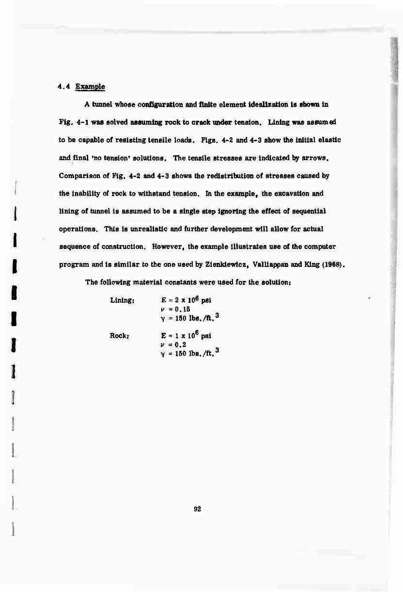
4.4 Example

A tunnel whose configuration and finite element idealization is shown in

Fig. 4-1 was solved assuming rock to crack under tension. Lining was assumed

to be capable of resisting tensile loads. Figs. 4-2 and 4-3 show the initial elastic

and final »no tension* solutions. The tensile stresses are indicated by arrows.

Comparison of Fig. 4-2 and 4-3 shows the redistribution of stresses caused by

the inability of rock to withstand tension. In the examplef the excavation and

lining of tunnel is assumed to be a single step ignoring the effect of sequential

operations. This is unrealistic and further development will allow for actual

sequence of construction. However, the example illustrates use of the computer

I program and is similar to the one used by Zlenkiewicz, Valliappan and King (1968).

The following material constants were used for the solution:

' Lining: E = 2 x 106 psi Iv =0.15

Y = 150 lbs./ft.

1 1 I .

I

3

Rock: E = 1 x 106 psi v =0.2 V = 150 lbs./ft.3

92

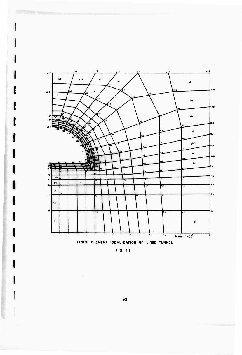
I

I I r-»

FINITE ELEMENT IDEALIZATION OF LINED 1UNNCL

FiG. 41

Scalt'T-lo'

93

\

Scale for Stresses

-f. 1" 10,000 psf Arrows for Tension

+

ELASTIC SOLUTION FOR THE LINED TUNNEL

FIG. 4.2

94

I

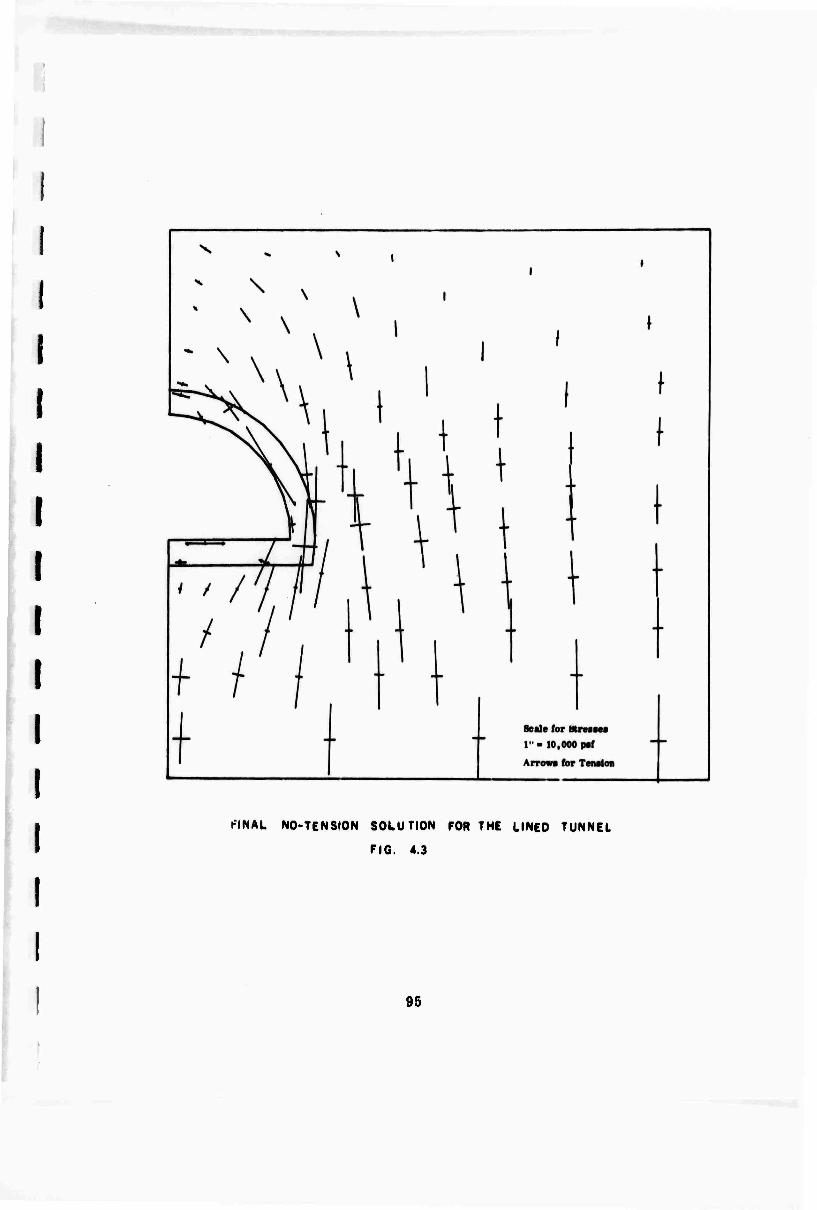
i I I

KINAL NO-TENSION SOLUTION FOR THE LINED TUNNEL

FIG. 4.3

95

CHAPTER V

ADDITIONAL COMMENTS

Chapter V. Additional Comments

The work reported Is continuing and significant changes may be made

before the finite element computer programs reach their final form. In the

case of elastic-plastic materials following Mohr-Coulomb Theory non-monotonic

loads have to be allowed for and also alternative numerical solution procedures

have to be examined. For the case of jointed rock the program included in the

report represents a necessary first step. Modification to include the Griffith

failure criterion is being done. For Griffith rupture caused by a tensile stress

field acting on pre-existing flaws, the solution scheme appears to be fairly

straight forward. However, the case of fracture under compressive stress

fields may require development of new methods.

96

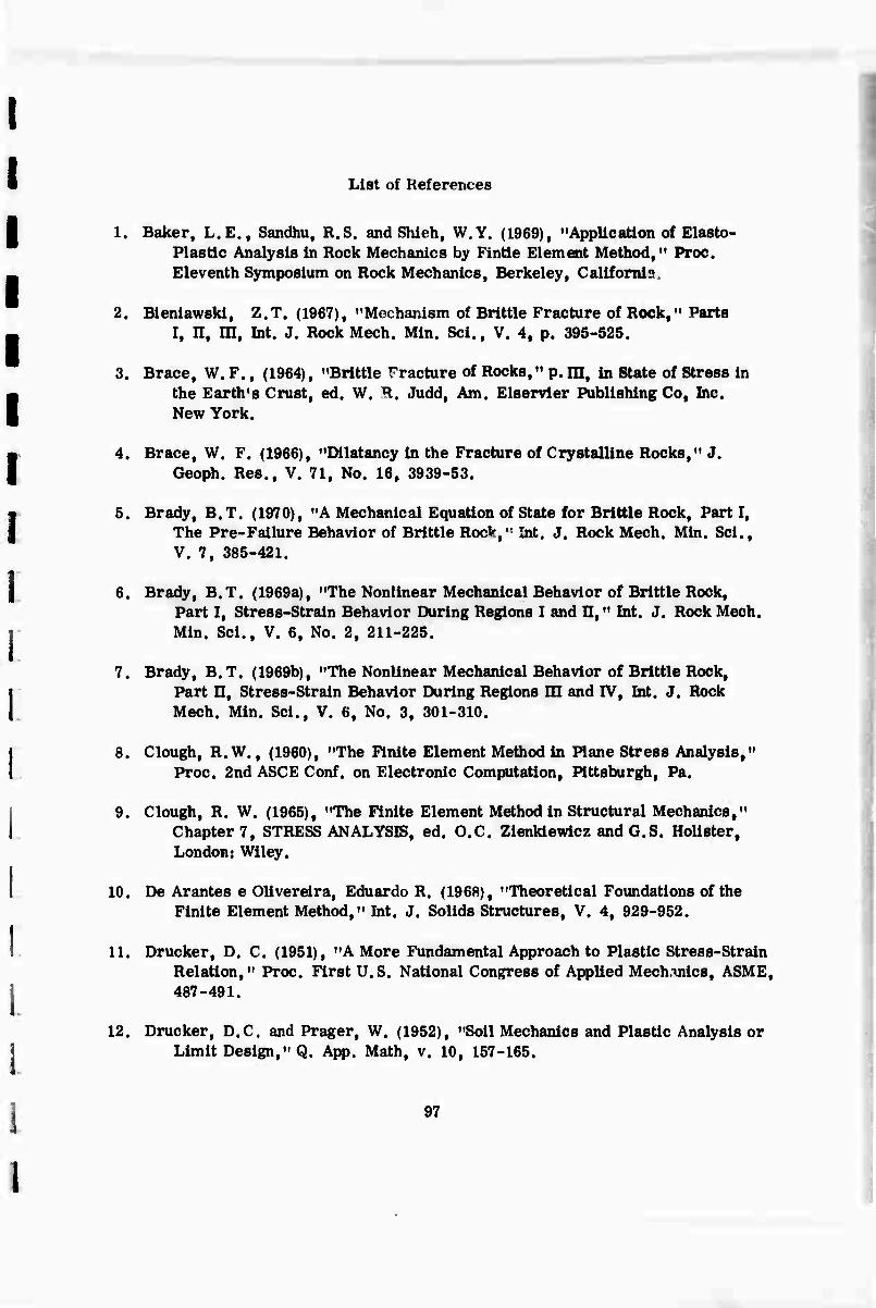
List of References

1. Baker, L.E., Sandhu, R.S. and Shleh, W.Y. (1969), "Application of Elasto- Plastic Analysis in Rock Mechanics by Fintte Element Method,** Proc. Eleventh Symposium on Rock Mechanics, Berkeley, Calif onus.

2. Bieniawski, Z.T. (1967), "Mechanism of Brittle Fracture of Rock," Parts I, n, in, Int. J. RockMech. Min. Sei., V. 4, p. 395-525.

3. Brace, W.F., (1964), "Brittle Fracture of Rocks,*' p.m, in State of Stress in the Earth's Crust, ed. W. R. Judd, Am. Eiservier Publishing Co, Inc. New York.

4. Brace, W. F. (1966), "Dilatancy in the Fracture of Crystalline Rocks," J. Geoph. Res., V. 71, No. 16, 3939-53.

5. Brady, B.T. (1970), "A Mechanical Equation of State for Brittle Rock, Part I, The Pre-Failure Behavior of Brittle Rock," Int. J. Rock Mech. Min. Sei., V. 7, 385-421.

6. Brady, B.T. (1969a), "The Nonlinear Mechanical Behavior of Brittle Rock, Part I, Stress-Strain Behavior During Regions I and n, ** bit. J. Rock Mech. Min. Sei., V. 6, No. 2, 211-225.

7. Brady, B.T. (1969b), "The Nonlinear Mechanical Behavior of Brittle Rock, Part 11, Stress-Strain Behavior During Regions HI and IV, Int. J. Rock Mech. Min. Sei., V. 6, No. 3, 301-310.

8. Clough, R. W., (1960), "The Finite Element Method in Plane Stress Analysis," Proc. 2nd ASCE Conf. on Electronic Computation, Pittsburgh, Pa.

9. Clough, R. W. (1965), "The Finite Element Method in Structural Mechanics,*' Chapter 7, STRESS ANALYSIS, ed. O.C. Zienkiewlcz and G.S. Holister, London: Wiley.

10. De Arantes e Olivereira, Eduardo R. (1968), "Theoretical Foundations of the Finite Element Method," Int. J. Solids Structures, V. 4, 929-952.

11. Drucker, D. C. (1951), "A More Fundamental Approach to Plastic Stress-Strain Relation," Proc. First U.S. National Congress of Applied Mechanics, ASME, 487-491.

12. Drucker, D.C. and Prager, W. (1952), "Soil Mechanics and Plastic Analysis or Limit Design," Q. App. Math, v. 10, 157-165.

13. Drucker, D. C.f Gibson, R. E. and Henkel, D.J. (1955), "Soil Mechanics and Work-Hardening Theories of Plasticltv." Paper No. 2864, Trans., ASCE.

14. Duncan, J.M. and Goodman, R.E. (1968), "Finite Element Analysis of Slopes in Jointed Rock," Report No. TE-68-1, U.S. Army Engineer Waterways Exp. Station, Corps of Engineers.

15. Einstein, H.H. , Bruhn, R.W. and Hirschfeld, R.C. (1970), "Mechanics of Jointed Rock, Experimental and Theoretical Studies," Soil Mech. Publication No. 268 M. I. T.

16. Felippa, C. (1966), "Refined Finite Element Analysis of Linear and Nonlinear Two-Dimensional Structures," Ph.D. Thesis, University of California, Berkeley.

17. Felippa, C.A. and Clough, R.W., "The Finite Element Method it\ Soiid Mechanics," V.2, SIAM-AMS Proc., Numerical Solution of Field Problems in Continuum Physics, Am. Math. Soc., Providence, R.I.

18. Goodman, R. E., Taylor, R.L. and Brekke, T.L. (1968), "A Model for the Mechanics of Jointed Rock," ASCE, SM3, 637-658.

19. Green, A.E. and Naghdi, P.M. (1965), "A General Theory of an Elastic- Plastic Continuum," Arch. Rational Mech. Anal, V. 18, 251-281.

20. Hill, R. (1950), The Mathematical Theory of Plasticity. Oxford University Press.

21. Holand and Bell (1970), "Finite Element Methods in Stress Analysis," TAPER, The Technical University of Norway, Trondheim, Norway, 2nd print.

22. Kolter, W.T. (1953), "Stress-Strain Relations, Uniqueness and Variational Theorems for Elastic-Plastic Materials with a Singular Yield Surface," Quar. Appl. Math. Vol. 11, 350-354.

23. Malina, H. (1970), "The Numerical Determination of Stresses and Deformations in Rock Taking into Account Discontinuities," Rock Mechanics 2, 1-16.

24. Melosh, R. J. (1963), "Basis for Derivation of Matrices for the Direct Stiffness Method," AIAA, V. 1, No. 7.

98

25. Naghdi, P.M. (1960), "Stress-Strain Relations in Plasticity and Thermo- plasticity," Plasticity: Proceedings of the 2nd Symposium on Naval Structural Mechanics, Pergman Press, 121-169.

26. Oden, J.T. (1969), "A General Theory of Finite Elements, I. Topological Considerations; 11. Applications, Int. J. Num. Math. Eng., V. 1, 205-221, 247-259.

27. Plan, T.H.H., (1968), "Variational Principles aiid Their Application to Finite Element Methods," Lecture Notes on "Finite Element Methods in Solid Mechanics," 24-38, M.I.T.

28. Prager, W. (1949), "Recent Developments in the Mathematical Theory of Plasticity," J. App. Phys., V. 20, p. 235.

29. Proc. Conf. Matrix Methods in Structural Mechanics, Wright-Patterson Air Force Base, Ohio, 1965.

30. Proc. 2nd Conf. on Matrix Methods in Structural Mechanics, AFFDL-TR- 68-150, Wright Patterson AFB, Ohio, 1968.

31. Reyes, S.F. (1965), "Elasto-Plastic Analysis of Underground Openings by the Finite Element Method," Ph.D. Thesis, University of Illinois.

32. Reyes, S.F. and Deere, D.V. (1966), "Elastic-Plastic Analysis of Under- ground Openings by Finite Element Method," Proc., First Congress International Society of Rock-Mechanics, Lisbon.

33. Sandhu, R.S. and Wilson, E.L. (1970), "Finite Element Analysis of Stresses in Mass Concrete Structures," Preprint, Symposium on Impact of Computers on the Practice of Structural Engineering in Concrete, ACI, St. Louis, Missouri.

34. Swanson, S.R. (1970), "Development of Constitutive Equations for Rocks," Ph. D. Thesis, University of Utah.

35. Walsh, J. B. (1965a), "The Effect of Cracks on the Compressibility of Rock," J. Geophys. Res., V. 70, No. 2, 381-389.

36. Walsh, J.B. (1965b), "The Effect of Cracks on the Uniaxial Elastic Com- pression of Rocks," J. Geophys. Res., V. 70, No. 2, 399-411.

99

37. Walsh, J. B. (1965c), "The Effect of Cracks in Rocks on Poisson's Ratio," J. Geophysical Res., V. 70, N. 20, 5249-57.

38. Wilson, E.L. (1963), "Finite Element Method in Two-Dimensional Problems," D. Engg. Thesis, University of California, Berkeley.

39. Wilson, E.L. (1965), "Structural Analysis of Axisymmetric Solids," J. AIAA, V. 3.

40. Yamada, Y., Yoshimura, N., and Sakurai, T. (1968), "Plastic Stress-Strain Matrix and its Application for Solution of Elastic-Plastic Problems by the Finite Element Method," Int. J, Mech. Sei. , Pergamon Press, V. 10, 343-354.

41. Zienkiewlcz, O.C. and Cheung, Y.K., (1967), The Finite Element Method in Structural and Continuum Mechanics. McGraw-Hill.

42. Zienkiewicz, O.C, Valliappan and King, I.P. (1969), "Elasto-Plastic Solutions of Engineering Problems, Initial Stress, Finite Element Approach," International Journal of Numberical Methods in Engg., V. 1, 75-100.

43. Zienkiewicz, O.C, Valliappan, S., and King, I.P. (1968), "Stress Analysis of Rock as a 'No Tension* Material," Geotechnique 18, No. 1, 56-66.

44. Zlamal, M. (1968), "On the Finite Element Method," Numer. Math. 12, 394-409.

100