To

appe

arin

the

Jour

nalof

Com

puta

tion

alP

hysi

cs15

1(1

999)

114-

134

The Nose-Poincare Method for Constant Temperature MolecularDynamics

Stephen D. Bond∗, Benedict J. Leimkuhler∗, and Brian B. Laird†∗ University of Kansas, Department of Mathematics, Lawrence, KS 66045, USA , † University of

Kansas, Department of Chemistry, Lawrence, KS 66045, USA

Version: November 15, 1998

We present a new extended phase space method for constant temperature (canonical ensemble) molecular

dynamics. Our starting point is the extended Hamiltonian introduced by Nose to generate trajectories corre-

sponding to configurations in the canonical ensemble. Using a Poincare time-transformation, we construct a

Hamiltonian system with the correct intrinsic timescale and show that it generates trajectories in the canonical

ensemble. Our approach corrects a serious deficiency of the standard change of variables (Nose-Hoover dynamics),

which yields a time-reversible system but simultaneously destroys the Hamiltonian structure. A symplectic dis-

cretization method is presented for solving the Nose-Poincare equations. The method is explicit and preserves the

time-reversal symmetry. In numerical experiments, it is shown that the new method exhibits enhanced stability

when the temperature fluctuation is large. Extensions are presented for Nose chains, holonomic constraints, and

rigid bodies.

1. INTRODUCTION

Molecular-dynamics computer simulation [1, 2] has become a standard tool in computational bio-physics and chemistry. Traditional molecular dynamics samples configurations from a constant energyor microcanonical distribution. This is often inappropriate since experiments are usually performed atconstant temperature (canonical ensemble). While Monte Carlo methods can be used for the canonicalensemble, these methods cannot be used to recover dynamical quantities and time-correlated functions.Hybrid methods using stochastics with molecular dynamics [3] can be used to generate the correct distri-butions, but they fail to provide correct dynamical quantities due to the discontinuous, stochastic changesin the flow. Methods using ad hoc non-reversible temperature controls [4], and isokinetic constraints [5–7]have also been proposed in the literature. These methods succeed in producing smooth trajectories, butthey fail to yield the correct canonical fluctuations in the kinetic energy [1]. This paper will focus on thenewer dynamical methods derived from the extended Hamiltonian proposed by Nose [8, 9]:

HNose =∑

i

p2i

2mi s2+ V (q) +

π2

2Q+ g k T ln s. (1)

Here g = Nf + 1, where Nf is the number of degrees of freedom of the real system. The constants T andk are temperature and Boltzmann’s constant respectively. An extended position variable, s, is introducedalong with its canonical momenta, π. The constant Q represents an artificial “mass” associated with s.One should note that p is the canonical momenta assosciated with the position variable, q. The accentis used to distinguish it from the from the real momenta given by p = p/s.

Nose proved that this system generates configurations from the canonical ensemble, provided that thedynamics is ergodic. He also showed that the intrinsic time variable must be rescaled to provide trajec-tories at evenly spaced points in real-time. Using data at unevenly spaced points in time does not causeany difficulties in the computation of ensemble averages, but it does significantly effect the computationof correlation functions. This difficulty is traditionally resolved using a real-variable formulation of theequations called Nose-Hoover [9, 10]. In this approach, the equations of motion are reformulated using anoncanonical change of variables. (Note that, in this paper the word canonical has two different meaningsdepending on context. With respect to statistical mechanical distributions, canonical refers to constanttemperature, whereas a canonical change of variables is one that leaves the form of Hamilton’s equationsinvariant.) Although the Nose-Hoover equations produce canonically distributed configurations, and thedynamics evolve with respect to real-time, the resulting system is not Hamiltonian. It does have a con-served quantity which is similar to energy, but the equations of motion do not arise from a corresponding

1

To

appe

arin

the

Jour

nalof

Com

puta

tion

alP

hysi

cs15

1(1

999)

114-

134

Poisson bracket (see [11], p. 320). Although the flow is time-reversible, it does not have a canonicalsymplectic structure.

The importance of time-reversibility and symplecticness in numerical integrators has recently becomea popular topic of discussion [12, 13]. A Hamiltonian system is time-reversible if it is an even functionof the momenta, which is the case in classical molecular dynamics. One says the flow of a canonicalHamiltonian system is symplectic since the solution operator preserves the wedge product of differentials,dp ∧ dq =

∑dpi ∧ dqi. In other words, the sum of oriented areas formed by projections of a 2-surface

in phase space onto the piqi coordinate planes is a first integral of the flow [14]. Recently a volume-preserving generalization of the Nose-Hoover method has been proposed [15]. While this was a significantachievement, one should note that symplecticness is a stronger property than the (phase space) volumepreservation provided by Liouville’s theorem. It is only in the special case of one degree of freedomsystems, that symplecticness is equivalent to area or volume conservation.

For a numerical integrator the symplectic property has a slightly different consequence. A numericalmethod is a discrete map (actually a family of maps parameterized by a stepsize ∆t) which can be viewedas a transformation of phase space. If one step of the method maps the point (qn, pn) to

(qn+1, pn+1

),

then the method is symplectic if dpn ∧ dqn = dpn+1 ∧ dqn+1. One can apply backward error analysis tosymplectic methods designed to approximate the dynamics of Hamiltonian systems [16, 17]. In this caseit can be shown that the numerical solution is the exact solution of a “nearby” Hamiltonian system, upto an exponentially small error. The Hamiltonian corresponding to the nearby system is obtained in theform of an asymptotic expansion.

Time-reversal symmetry and symplecticness are both strong geometric properties of the flow of adynamical system. However time-reversal symmetry of a numerical method does not in general providean approximate conserved energy integral obtainable through an asymptotic expansion, as is availablefor symplectic methods [17]. Near conservation of energy over long time intervals is a direct resultof this approximately conserved quantity. While time-reversible methods will show the same type ofstability near the symmetry plane (p = 0), there is no guarantee that this will be the case far from thesymmetry plane (at high temperatures) [18]. In addition to stability issues, the use of algorithms whichare volume-preserving and time-reversible is required for hybrid Monte Carlo methods [19].

In this paper we will show that it is possible to derive a time-reversible, real-time formulation withoutsacrificing the symplectic structure. This new approach uses a new extended Hamiltonian which we callNose-Poincare,

H =

(∑i

p2i

2mi s2+ V (q) +

π2

2Q+ g k T ln s−H0

)s. (2)

Now the constant g = Nf , the number of degrees of freedom of the real system. This Hamiltoniansystem is related to the Nose system through a Poincare transformation of time [20–22]. The value ofthe constant H0 is chosen such that H is zero when evaluated at the initial conditions. We will alsoshow that the dynamics of the Nose-Poincare system can be integrated explicitly using a new symplectic,time-reversible integrator.

In Section 2 we discuss the Nose-Hoover approach to reformulating the Nose Hamiltonian in real-variables. We review two of the numerical methods which have been previously proposed for solving theNose-Hoover equations [1,23–25]. In Section 3 we introduce a new symplectic, time-reversible integratorfor Nose-Poincare. We verify that it generates configurations from the correct distribution, and formu-late an appropriate numerical method for propagating the dynamics. Using numerical experiments inSection 4, we compare the Nose-Poincare method with two popular methods for Nose-Hoover. Theseexperiments indicate that the Nose-Poincare method has better stability properties in simulations withlarge fluctuations of the thermostat variable, s. This situation arises when the extended “mass”, Q, ismade small to increase sampling speed, or when the initial conditions are not properly equilibrated tothe simulation temperature. In the Appendices we discuss the extensions of the Nose-Poincare approachto Nose chains, holonomic constraints, and rigid bodies.

2. THE NOSE HAMILTONIAN AND NOSE-HOOVER METHOD

Although the Nose Hamiltonian generates configurations from the canonical distribution, it also in-troduces an unnatural scaling of the intrinsic time. This introduces computational difficulties, since theconfigurations are not available at equally spaced points in real-time. A real-variable reformulation ofthe equations of motion was proposed by Nose [8, 9] to remedy this problem. Simplifications to the

2

To

appe

arin

the

Jour

nalof

Com

puta

tion

alP

hysi

cs15

1(1

999)

114-

134

real-variable system were proposed by Hoover [10] resulting in the traditional treatment of the NoseHamiltonian called Nose-Hoover. In this section we review the Nose-Hoover system of equations, anddiscuss some of the common numerical methods [1, 23–25] proposed for solving them.

We begin with the equations of motion derived from the Nose Hamiltonian, (1),

dqidτ

=pi

mi s2,

ds

dτ=π

Q, (3)

dpi

dτ= − ∂

∂qiV (q) ,

dπ

dτ=∑

i

p2i

mi s3− g k T

s. (4)

Nose [9] has shown that the dynamics associated with this system generate canonically distributed con-figurations, p/s and q. To convert to real configurations, a non-canonical change of variables is used:

p =p

s, π =

π

s. (5)

This is followed by a Sundman time-transformation [20] applied to the vector field,

dτ

dt= s, (6)

resulting in a new system of non-Hamiltonian equations for the dynamics in the real variables:

qi =pi

mi, pi = − ∂

∂qiV (q)− pi

s π

Q, (7)

s =s2 π

Q, ˙π =

1s

(∑i

p2i

mi− g k T

)− s π2

Q. (8)

Hoover [10] noted that the equations could be simplified considerably since π and s always appear together.By making another change of variables from π to ξ = s π/Q and from ln s to η, one not only eliminates thevariable π, but also decouples the variable s from the system. This results in the Nose-Hoover equationsfor the dynamics in reduced real-variable formulation:

qi =pi

mi, pi = − ∂

∂qiV (q)− pi ξ, (9)

η = ξ, ξ =1Q

(∑i

p2i

mi− g k T

). (10)

In the reduced system the constant g = Nf (the number of degrees of freedom of the real system) asopposed to g = Nf + 1 in the Nose formulation. This reduction in the degrees of freedom is needed torecover configurations at the correct temperature [9]. Although this system is not Hamiltonian, it doeshave a conserved quantity, which we call the total extended energy:

Eext =∑

i

p2i

2mi+ V (q) +

Qξ2

2+ g k T η. (11)

The application of a Sundman time-transformation necessarily destroys the canonical symplectic structure[26]. It is for this reason that the Nose-Hoover system in (9)-(10) does not have such a structure.

This system is time-reversible, and it is advisable to solve the equations of motion with a reversibleintegrator. We will now explore two of the more commonly used reversible methods, both of which arebased on variants of the generalized leapfrog algorithm [25].

The first is an implicit method [1] based on a modification of the velocity Verlet algorithm. It consistsof alternating explicit and implicit half-steps with the momenta variables, with explicit whole-steps inthe position variables. The method is given below in a whole-step formulation, i.e. as a mapping fromtime tn to tn+1 = tn + ∆t:

3

To

appe

arin

the

Jour

nalof

Com

puta

tion

alP

hysi

cs15

1(1

999)

114-

134

pn+1/2i = pn

i −∆t2

(∂

∂qiV (qn) + ξnpn

i

), (12a)

ξn+1/2 = ξn +∆t2Q

(∑i

(pni )2

mi− g k T

), (12b)

qn+1i = qn

i + ∆tp

n+1/2i

mi, (12c)

ηn+1 = ηn + ∆tξn+1/2, (12d)

pn+1i = p

n+1/2i − ∆t

2

(∂

∂qiV(qn+1

)+ ξn+1pn+1

i

), (12e)

ξn+1 = ξn+1/2 +∆t2Q

(∑i

(pn+1

i

)2mi

− g k T

). (12f)

Equations (12e) and (12f) are implicitly coupled and must be solved together. Traditionally, thisstep is solved with a 3N + 1 dimensional Newton iteration [1]. This can be simplified considerably bysubstitution, eliminating pn+1 from the iteration. This results in a scalar-cubic equation in terms of ξn+1

and can be solved either directly or using a simple iterative method.Several explicit time-reversible methods have been proposed for the Nose-Hoover equations [23–25].

The second method which we consider in this paper [23, 25] is one which is explicit, and based on theStormer-Verlet method. We write it in its leapfrog form for comparison purposes:

pn+1/2i = pn

i −∆t2

(∂

∂qiV (qn) + ξnp

n+1/2i

), (13a)

qn+1i = qn

i + ∆tp

n+1/2i

mi, (13b)

ξn+1 = ξn +∆tQ

∑i

(p

n+1/2i

)2

mi− g k T

, (13c)

ηn+1 = ηn +∆t2(ξn+1 + ξn

), (13d)

pn+1i = p

n+1/2i − ∆t

2

(∂

∂qiV(qn+1

)+ ξn+1p

n+1/2i

). (13e)

3. THE NOSE-POINCARE METHOD

As we illustrated in the previous section, the traditional real-variable formulation of Nose-Hooverdestroys the symplectic structure associated with the Nose Hamiltonian. In this section we will outlinea procedure for scaling time while preserving the Hamiltonian structure. The method proposed in thispaper is formulated through a Poincare transformation [20] of the Hamiltonian H = H(q, p):

H = f(q, p)(H−H0), f > 0, (14)

where f is a “time scaling” function, and the constant H0 is the initial value of H. Along the energy sliceH = H0, the dynamics of the transformed system will be equivalent to those of the original system, upto a transformation of time. To see this, write the Hamilton equations of motion

qi = f∂

∂piH+ (H−H0)

∂

∂pif, (15)

pi = −f ∂

∂qiH− (H−H0)

∂

∂qif, (16)

4

To

appe

arin

the

Jour

nalof

Com

puta

tion

alP

hysi

cs15

1(1

999)

114-

134

then observe that when H = H0, the equations are the same as the original equations expressed in thereal-time variable, t, related to τ by

dτ

dt= f(q, p). (17)

Now we consider the Poincare transformation, f (q, p) = s, applied to a slightly modified version ofthe Nose extended Hamiltonian in (1):

H = (HNose −H0) s, (18)

H =

(∑i

p2i

2mi s2+ V (q) +

π2

2Q+ g k T ln s−H0

)s. (19)

The modification comes in that we are using the constant g = Nf (as opposed to g = Nf + 1). We willsee later that this small change is necessary for the correct distribution of configurations. The constantH0 is chosen to be the initial value of the Nose Hamiltonian, HNose. We will show that this transformedHamiltonian in (2) and (19), which we call Nose-Poincare, generates configurations from the canonicaldistribution in the variables q and p/s.

Theorem: The Nose-Poincare system generates canonically distributed averages, given the usual statis-tical mechanics assumptions of equal a priori probabilities and ergodicity.

The proof will involve derivation of the probability distribution, and partition function for the Nose-Poincare Hamiltonian.Proof: Consider the probability of finding a particular configuration in the phase-space described by thereal variables, (q, p):

dq dp F (q, p) ≡∫

dπ∫

ds dp dq Fext (q, p, s, π) . (20)

For the Nose-Poincare Hamiltonian, H, we can write the probability of finding a particular configurationof energy H0 as a microcanonical distribution in the extended phase space, (q, p, s, π):

dπ ds dp dq Fext (q, p, s, π) =dπ ds dp dq δ

[H − H0

]∫

dπ∫

ds∫

dp∫

dq δ[H − H0

] . (21)

In the above expression the usual statistical mechanical assumptions of equal a priori probabilities andergodic (or quasi-ergodic) dynamics are made [27]. We now subsititute (21) in the expression (20),resulting in

dq dp F (q, p) =1

Z N !hNf

∫dπ∫

ds dp dq δ[H − H0

], (22)

where the Nose-Poincare partition function is given by

Z =1

N !hNf

∫dπ∫

ds∫

dp∫

dq δ[H − H0

]. (23)

Using H0 = 0, and expanding H, we get

dq dp F (q, p) =1

Z N !hNf

∫dπ∫

ds dp dq δ[s (HNose −H0)] , (24)

If we let H (p, q) =∑

ip2

i

2 mi+ V (q), this reduces to

dq dp F (q, p) =1

Z N !hNf

∫dπ∫

ds dp dq δ[s

(H (p/s, q) +

π2

2Q+ g k T ln s−H0

)]. (25)

Since s is strictly positive, we can make the change of variables p← p/s, yielding

dq dp F (q, p) =1

Z N !hNf

∫dπ∫

ds dp dq sNf δ

[s

(H (p, q) +

π2

2Q+ g k T ln s−H0

)]. (26)

5

To

appe

arin

the

Jour

nalof

Com

puta

tion

alP

hysi

cs15

1(1

999)

114-

134

Whenever a smooth function, r (s), has a single simple root at s = s0, one can write the relation δ [r(s)] =δ [s− s0] / |r′ (s0)|. This relation can be directly applied to (26), resulting in following expression:

δ

[s

(H (p, q) +

π2

2Q+ g k T ln s−H0

)]=

1|g k T |

δ

[s− exp

(−1g k T

(H (p, q) +

π2

2Q−H0

))]. (27)

These substitutions transform (26) into the following:

dq dp F (q, p) =1

Z N !hNf

∫dπ∫

ds dp dqsNf

g k Tδ

[s− exp

(−1g k T

(H (p, q) +

π2

2Q−H0

))]. (28)

Integrating over s, and substituting for the root s0, results in

dq dp F (q, p) =1

Z N !hNf g k Texp

(NfH0

g k T

)∫dπ dq dp exp

(−Nf

g k T

(H (p, q) +

π2

2Q

)). (29)

Finally, let g = Nf , and integrate over π to reduce the equation to:

dq dp F (q, p) =C

Z N !hNfdq dp exp

(− 1k T

H (p, q)), (30)

where C is a positive constant. The above procedure can also be applied to Z, which can be thensubstituted along with (30) into (22). After canceling the prefactor C/(N !hNf ) we have shown that

dq dp F (q, p) =dq dp exp

(− 1

k T H (p, q))∫

dq∫

dp exp(− 1

k T H (p, q)) . (31)

Since the righthand side of the expression is the probability of finding a configuration in the canonicalensemble, this completes the proof. If as is the usual case in molecular dynamics that total linear momen-tum is conserved, then an additional restriction of zero total linear momentum is required [9,10,28,29]. �

The disadvantage of the general Poincare transformation in (14) is that it mixes the variables sothat an explicit symplectic treatment of the extended Hamiltonian is not, in general, possible and oneis compelled to use implicit symplectic methods (see [21, 22]). However, this is not always the case fortransformation functions, f (q, p), which depend only on a reduced number of the phase-space variables(i.e. f (q) or f (s)). In these special cases, the variables are sufficiently decoupled, and we can easilyformulate explicit symplectic methods [16,30].

Returning to the Nose-Poincare Hamiltonian, H, we write the equations of motion:

qi =pi

mi s, ˙pi = −s ∂

∂qiV (q) , (32)

s = sπ

Q, π =

∑i

p2i

mi s2− g k T −∆H (q, p, s, π) , (33)

∆H (q, p, s, π) =∑

i

p2i

2mi s2+ V (q) +

π2

2Q+ g k T ln s−H0. (34)

The value of H0 is chosen such that ∆H (q0, p0, s0, π0) = 0. A simple method for numerically solving theNose-Poincare equations of motion is the generalized leapfrog algorithm [16,30]. Since we are treating aHamiltonian system, the resulting method is symplectic and time-reversible [13,21,22].

pn+1/2i = pn

i −∆t2sn ∂

∂qiV (qn) , (35a)

πn+1/2 = πn +∆t2

∑i

1mi

(p

n+1/2i

sn

)2

− g k T

− ∆t2

∆H(qn, pn+1/2, sn, πn+1/2

), (35b)

sn+1 = sn +∆t2(sn+1 + sn

) πn+1/2

Q, (35c)

6

To

appe

arin

the

Jour

nalof

Com

puta

tion

alP

hysi

cs15

1(1

999)

114-

134

qn+1i = qn

i +∆t2

(1

sn+1+

1sn

)p

n+1/2i

mi, (35d)

πn+1 = πn+1/2 +∆t2

∑i

1mi

(p

n+1/2i

sn+1

)2

− g k T

− ∆t2

∆H(qn+1, pn+1/2, sn+1, πn+1/2

),(35e)

pn+1i = p

n+1/2i − ∆t

2sn+1 ∂

∂qiV(qn+1

). (35f)

Due to the special structure of the system, the resulting method is also explicit. Note that (35b)requires the solution of a scalar quadratic equation for πn+1/2:

∆t4Q

(πn+1/2

)2

+ πn+1/2 + C = 0, (36)

where

C =∆t2

g k T (1 + ln sn)−∑

i

(p

n+1/2i

)2

2mi (sn)2+ V (qn)−H0

− πn. (37)

In this simplified formulation, C is a constant which can be easily computed. This equation can be solvedexplicitly using the quadratic formula, but one should be careful to solve for the correct root. To avoidsubtractive cancellation in the computation, we use a variant of the quadratic formula to solve (36):

πn+1/2 =−2C

1 +√

1− C∆t/Q(38)

The remaining steps in the algorithm are completely explicit, and can be solved sequentially.

4. NUMERICAL EXPERIMENT: LENNARD-JONES FLUID

As a numerical experiment, we compare the two proposed Nose-Hoover methods with the Nose-Poincare method. As a test problem, we consider 108 particles in cubic periodic box, using the minimumimage convention. A truncated, shifted and smoothed Lennard-Jones potential is used. It is importantthat the potential is smoothly truncated to zero to prevent artificial energy jumps [31]. Our experimentshave indicated that the potential function should be at least C2, i.e. it has a continuous second derivative.We find this higher degree of smoothness is important in some systems for verifying the order of thenumerical methods. The resulting smoothed pair-potential function is as follows:

VLJ (r) ={S (r) (VLJ (r)− VLJ (rc)) r ≤ rc

0 r > rc, (39)

where

VLJ (r) = 4ε((σ

r

)12

−(σr

)6). (40)

The smoothing function S (r) is defined by

S (r) = 1− 3(r

rc

)2

+ 3(r

rc

)4

−(r

rc

)6

. (41)

We give all of the results of our numerical experiments in reduced units. Specifically, we will use σ, ε,and m as the basic units of length, energy, and mass, respectively. In addition to the basic units, we willbe using reduced temperature (T ∗ = kTε−1), density (ρ∗ = ρσ3), and time (t∗ = tσε1/2m−1/2). All of oursimulations are performed with total linear momenta set to zero, hence we set g = Nf with Nf = 3N − 3(see [8, 28]). In all of the numerical experiments, we set the initial conditions of the extended variablesto be s0 = 1 and π0 = 0. For this reason, the initial extended energy of the system is the same as theinitial energy of the real system. We define the relative extended energy error at time t as∣∣∣∣E (t)− E (0)

E (0)

∣∣∣∣ , (42)

7

To

appe

arin

the

Jour

nalof

Com

puta

tion

alP

hysi

cs15

1(1

999)

114-

134

−5 −4 −3 −2 −1 0 1 2 3 4 50

0.05

0.1

0.15

0.2

0.25

0.3

0.35

0.4

prob

abili

ty, P

(p)

momenta, p

Maxwell−BoltzmannVerlet (NVE) Nose−Hoover−Im Nose−Hoover−Ex Nose−Poincare

1 1.1 1.2 1.3 1.4 1.5 1.6 1.7 1.8 1.9 20

0.5

1

1.5

2

2.5

3

3.5

prob

abili

ty d

ensi

ty, P

(T)

temperature, T

Nose−Hoover−ImNose−Hoover−ExNose−Poincare

FIG. 1 Comparison of momenta and temperature distributions for a Lennard-Jones fluid (N = 108,T ∗ = 1.5, ρ∗ = 0.95). The squares, triangles, circles, and pluses are from trajectories generated by theimplicit Nose-Hoover, explicit Nose-Hoover, Nose-Poincare, and traditional Verlet methods respectively.On the left, the momenta distribution is compared with the Maxwell-Boltzmann distribution (solid line).On the right, the distribution of the instantaneous temperature is shown. A Gaussian is fit to each curveto highlight the statistical similarities.

where the quantity E is determined by H , Eext, and HNose when using the Verlet, Nose-Hoover, andNose-Poincare methods respectively (see Sections 2 and 3 for details).

In our first experiment, we start the simulation equilibrated to T ∗ = 1.5, with ρ∗ = 0.95, andQ = 1.0. The timestep is set relatively low (∆t∗ = 0.005), to verify the qualitative behavior of themethods in a numerically stable regime. In Figure 1 the distribution of the momenta is compared withthe Maxwell-Boltzmann distribution for this temperature. We also show the results from the Verletmethod (traditional molecular dynamics), which does not use a temperature control. For this method,the simulation temperature cannot be determined until the simulation is complete. A tedious trial-and-error process had to be used to find initial conditions which would yield the correct temperature. It isthis exact reason why the Nose methods are preferred to traditional molecular dynamics for generatingconfigurations at constant temperature. As expected all four methods generated Boltzmann distributedmomenta, since the system is ergodic. We also show the distribution of the instantaneous temperaturefor the Nose methods. All three generate Gaussian distributed temperatures with the same mean andvariance.

We now investigate the behavior of the methods with respect to dynamical quantities associatedwith time-correlated functions. In Figure 2 we show the velocity autocorrelation function and mean-square displacement as functions of time. All four methods give almost identical results for both of thesefunctions. This indicates that the dynamics associated with Nose-Hoover and Nose-Poincare evolve withthe correct scale of time. We use the mean-square displacement curve to measure the diffusion coefficient,and note that all four curves asymptotically approach straight lines of equal slope. Fitting a line to thecurves in the asymptotic regime t∗ > 2.0, we calculate the diffusion coefficient D∗ ≈ 0.03. To checkthe reliability of this estimate, we calculated the same value by numerical integration of the normalizedautocorrelation curve. The two curves are related to one another through the Einstein and Green-Kuborelations [32],

D =1

2 dlim

t→∞

∆r2 (t)t

=k T

m

∫ ∞

0

< v (t) · v (0) >< v (0) · v (0) >

dt. (43)

The parameter Q plays an interesting role in determining the characteristics of Nose dynamics. In thelimit as Q goes to infinity the extended variable s remains constant, and we recover traditional moleculardynamics. Similarly, one can verify that both the Nose-Hoover and Nose-Poincare methods reduce toVerlet in this same limiting case. A drastically different situation arises when Q is small. This case is ofpractical interest since the rate at which configurational space is sampled can be increased by decreasingthe size of Q. However, one must be cautious not to make Q too small since this leads to high frequencyoscillations in s. This can lead to sampling problems, in addition to the computational difficulties. Thebest value for Q is problem dependent, and many authors have suggested that Q should be chosen inresonance with the real system to reduce “artificial effects” introduced by the thermostat [8–10,29,33,34].

8

To

appe

arin

the

Jour

nalof

Com

puta

tion

alP

hysi

cs15

1(1

999)

114-

134

0 0.1 0.2 0.3 0.4 0.5 0.6 0.7 0.8−0.2

0

0.2

0.4

0.6

0.8

1

time, t*

norm

aliz

ed v

eloc

ity a

utoc

orre

latio

n

Verlet (NVE) Nose−Hoover−ImNose−Hoover−ExNose−Poincare

10−2

10−1

100

101

10−2

10−1

100

101

time, t*

mea

n−sq

uare

dis

plac

emen

t, ∆

r(t)

2

Verlet (NVE) Nose−Hoover−ImNose−Hoover−ExNose−Poincare

FIG. 2 Comparison of time correlated quantities for a Lennard-Jones fluid (N = 108, T ∗ = 1.5, ρ∗ =0.95). The dotted, dashed, dashed-dotted, and solid lines are from trajectories generated by the implicitNose-Hoover, explicit Nose-Hoover, Nose-Poincare, and traditional Verlet methods respectively. On theleft, we show the normalized velocity autocorrelation function <v(t)·v(0)>

<v(0)·v(0)> . On the right, the mean-squaredisplacement is shown as a function of time.

10−3

10−2

10−4

10−3

10−2

10−1

100

max

imum

rel

ativ

e en

ergy

err

or

stepsize, dt

N = 108 ρ* = 0.95 tfinal

= 10.0 T* = 1.5 Q = 10.0

Verlet (NVE) Nose−Hoover−ImNose−Hoover−ExNose−Poincare

10−3

10−2

10−4

10−3

10−2

10−1

100

max

imum

rel

ativ

e en

ergy

err

or

stepsize, dt

N = 108 ρ* = 0.95 tfinal

= 10.0 T* = 6.0 Q = 10.0

Verlet (NVE) Nose−Hoover−ImNose−Hoover−ExNose−Poincare

FIG. 3 Comparison of extended energy conservation as a function of stepsize for a Lennard-Jones fluid(N = 108 and ρ∗ = 0.95). The maximum relative error in extended energy conservation is shown as afunction of stepsize. A relatively large value for the “extended mass” is used (Q = 10.0). On the left, thecurves are generated using a temperature of T ∗ = 1.5. On the right, a larger value of T ∗ = 6.0 is used.

9

To

appe

arin

the

Jour

nalof

Com

puta

tion

alP

hysi

cs15

1(1

999)

114-

134

10−3

10−2

10−4

10−3

10−2

10−1

100

101

max

imum

rel

ativ

e en

ergy

err

or

stepsize, dt

N = 108 ρ* = 0.95 tfinal

= 10.0 T* = 1.5 Q = 0.1

Verlet (NVE) Nose−Hoover−ImNose−Hoover−ExNose−Poincare

10−3

10−2

10−4

10−3

10−2

10−1

100

max

imum

rel

ativ

e en

ergy

err

or

stepsize, dt

N = 108 ρ* = 0.95 tfinal

= 10.0 T* = 6.0 Q = 0.1

Verlet (NVE) Nose−Hoover−ImNose−Hoover−ExNose−Poincare

FIG. 4 Comparison of extended energy conservation as a function of stepsize for a Lennard-Jones fluid(N = 108 and ρ∗ = 0.95). The maximum relative error in extended energy conservation is shown as afunction of stepsize. A relatively small value for the “extended mass” is used (Q = 0.1). On the left, thecurves are generated using a temperature of T ∗ = 1.5. On the right, a larger value of T ∗ = 6.0 is used.

As a second test, we consider the effects of changes in the extended mass, Q, on the stability of thealgorithms. We start with the case of a relatively large extended mass, Q = 10. Since the Nose-Hooverand Nose-Poincare methods reduce to Verlet as Q becomes large, we expect similar behavior for all of themethods. Each simulation is started with the system properly equilibrated to the simulation temperature.We follow the dynamics for a range of stepsizes between 0.002 and 0.02 while the final time is held fixedat 10 units. In Figure 3, the maximum relative error in the extended energy deviation is shown as afunction of stepsize for two different temperatures, T ∗ = 1.5 and T ∗ = 6.0. For clarity, only the valuesin the stable regime of each method are shown in the diagram. The method was considered unstableif the simulation temperature deviated by more than 5 percent from the target value of T ∗ = 1.5 orT ∗ = 6.0. For this particular case, there is no clear difference in the efficiency of the methods. All fourof the methods perform nearly the same for small stepsizes, as expected. However, for large stepsizes theimplicit Nose-Hoover method shows better stability properties. However, the magnitude of the error inthe energy at the larger stepsizes is a concern, as it can be an indication of non-physical behavior in thecomputed trajectory.

In Figure 4, the same efficiency diagrams are shown for Q = 0.1. Since the Verlet method does notuse the parameter Q, its results are the same as in the previous figure. For this smaller value of Q, theNose-Poincare method is slightly more efficient than the explicit Nose-Hoover method. While the implicitNose-Hoover method does show better stability at large stepsizes, it is more inefficient than the othermethods at smaller stepsizes. Our results indicate that the Nose-Hoover methods are less efficient whenthe parameter Q is small. This could be a result of the more rapid fluctuations in the thermostat.

To further investigate the effect of fluctuations in the thermostat, we now consider the same systemwith a jump in the target temperature. The parameter Q is set to 0.1, and the simulation is startedwith the system equilibrated to T ∗ = 1.5 and ρ∗ = 0.95. At t∗ = 0 the Nose thermostat is turned on,and the temperature is increased to T ∗ = 6.0. Due to the change in the system temperature, we areunable to use traditional molecular dynamics algorithms (i.e. Verlet) for this simulation. In Figure 5,the relative error in extended energy is shown as a function of stepsize. We also show the relative energyerror for a particular stepsize, ∆t = 0.006, near the stability limit. For all three of the algorithms, thereis a large initial jump due to the increase in the imposed temperature. However, for large stepsizes theNose-Poincare method is the most stable during this initial equilibration phase, and shows the smallestjump in energy. For very small stepsizes, the explicit Nose-Hoover method appears to be slightly moreefficient than Nose-Poincare.

Over longer time intervals, the difference becomes even more pronounced. In our last experiment,we follow the dynamics for 500000 steps at a stepsize of ∆t∗ = 0.006. The parameter Q is set to 0.1,and the simulation is started with the initial conditions equilibrated to the thermostat temperature of

10

To

appe

arin

the

Jour

nalof

Com

puta

tion

alP

hysi

cs15

1(1

999)

114-

134

10−3

10−2

10−2

10−1

100

101

102

max

imum

rel

ativ

e en

ergy

err

or

stepsize, dt

N = 108 ρ* = 0.95 tfinal

= 10.0 T* = 6.0 Q = 0.1

Nose−Hoover−ImNose−Hoover−ExNose−Poincare

0 0.5 1 1.5 2 2.5 3 3.5 4 4.5 510

−2

10−1

100

101

102

time, t*

rela

tive

ener

gy e

rror

Nose−Poincare

Nose−Hoover−Im

Nose−Hoover−Ex

N = 108 ρ* = 0.95 T* = 6.0 Q = 0.1 tfinal

= 10.0 ∆t = 0.006

FIG. 5 Simulation of a temperature jump in a Lennard-Jones fluid (N = 108, T ∗ = 6.0, ρ∗ = 0.95,Q = 0.1). The system was first equilibrated to T ∗ = 1.5 before the temperature was increased toT ∗ = 6.0 at t∗ = 0. On the left, the maximum relative error in the extended energy is shown as afunction of stepsize. On the right, the relative error in the extended energy is shown for a large stepsize(∆t∗ = 0.006).

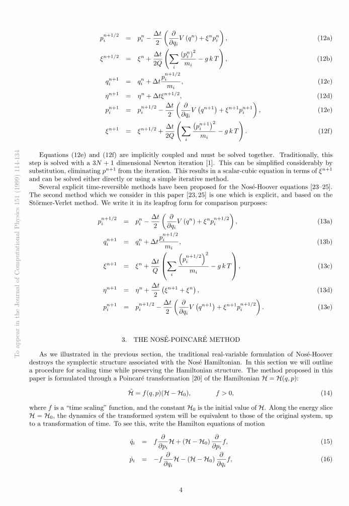
T ∗ = 6.0. In Figure 6, the relative energy error is shown as a function of time. All of the methods showsome drift in the energy, for this long time simulation. However, the extended energy is conserved muchbetter by the Nose-Poincare and Verlet methods. The Nose-Hoover methods, which are not symplectic,are destabilized by the large fluctuations in temperature due to the small value of Q.

5. CONCLUSIONS

We have presented a new method for constant temperature (canonical) molecular dynamics, calledNose-Poincare. The new method has a wide range of applications, including rigid bodies and Nosechains, while providing a symplectic framework for a real-time formulation of the Nose Hamiltonian.Although the traditional Nose-Hoover approach also provides a real-variable system, it does so througha noncanonical change of variables. While both approaches are time reversible, only Nose-Poincare has acanonical symplectic structure. Both time-reversible symmetry and symplecticness are strong geometricproperties of a dynamical flow. The difference is in that the reversible symmetry of a numerical methoddoes not in general provide an approximate integral obtainable through an asymptotic expansion of a“nearby Hamiltonian”. Near conservation of energy over long time intervals is a direct result of thisapproximately conserved quantity. While time-reversible methods will show the same type of stabilitynear the symmetry plane (p = 0), there is no guarantee that this will be the case far from the symmetryplane (|p| >> 0). This is one of the clear qualitative distinctions between symplectic and reversiblemethods.

Our numerical experiments have indicated that the Nose-Poincare formulation provides improvedstability in simulations with large fluctuations in the thermostat variable. This situation arises when theinitial temperature does not correspond to the simulation temperature, and when the parameter Q issmall. In this case, the Nose-Hoover methods show larger jumps in the extended energy for moderatelylarge stepsizes. One should also note that our experiments have shown no clear difference between theexplicit Nose-Hoover method and Nose-Poincare for very small stepsizes, and when the system is properlyequilibrated. The implicit Nose-Hoover method is more stable at large stepsizes than the explicit form, butit is not as efficient in achieving a given degree of accuracy. Our observation is that for moderately largestepsizes the Nose-Poincare method can be a substantially better method, and is certainly no worse thanthe Nose-Hoover formulation. Since the Nose-Poincare method is symplectic, as well as time-reversible,we recommend its use for constant temperature simulations.

11

To

appe

arin

the

Jour

nalof

Com

puta

tion

alP

hysi

cs15

1(1

999)

114-

134

0 1000 2000 30000

0.05

0.1

0.15

0.2

rela

tive

ener

gy e

rror

Nose−Hoover−Im

0 1000 2000 30000

0.05

0.1

0.15

0.2

rela

tive

ener

gy e

rror

time, t*

Nose−Poincare

0 1000 2000 30000

0.05

0.1

0.15

0.2Nose−Hoover−Ex

0 1000 2000 30000

0.05

0.1

0.15

0.2

time, t*

Verlet

FIG. 6 Long time simulation of a Lennard-Jones fluid (N = 108, T ∗ = 6.0, ρ∗ = 0.95, Q = 0.1). Thedynamics were followed for 500000 steps, at a stepsize of ∆t∗ = 0.006, with initial conditions equilibratedto T ∗ = 6.0. The relative error in the extended energy is shown as a function of stepsize for the variousmethods.

6. ACKNOWLEDGMENTS

The authors were supported by NSF Grant No. DMS-9627330. Simulations were performed oncomputers provided by KCASC and KITCS. The authors would also like to thank Gregory Voth forstimulating conversations.

APPENDIX A: NOSE CHAINS

It has been shown that the Nose Hamiltonian generates configurations from the canonical ensembleif the dynamics is ergodic [9,10,29]. The hypothesis of ergodicity can be violated in special cases [29,34](i.e. small systems and systems with stiff springs). A simple extension of the Nose-Hoover equations hasbeen developed, called Nose-Hoover chains [33], which alleviates this ergodicity problem. This methodinvolves introducing a sequence of new thermostats, each one coupled to the previous, resulting in a chain.The Nose-Hoover chain equations are implicitly coupled, but can be solved explicitly using an even-oddsplitting [24, 25]. To derive the equations for the chains, one starts with the Nose-Hoover equations asdefined in (9)-(10),

qi =pi

mi, pi = − ∂

∂qiV (q)− pi

ϕ

Q, (44)

η =ϕ

Q, ϕ =

∑i

p2i

mi− g k T. (45)

Here the variable ϕ is equivalent to Qξ in equations (9-10). Now J − 1 new thermostats are introduced,each one coupled to the previous, resulting in a Nose-Hoover chain:

qi =pi

mi, pi = − ∂

∂qiV (q)− pi

ϕ1

Q1, (46)

12

To

appe

arin

the

Jour

nalof

Com

puta

tion

alP

hysi

cs15

1(1

999)

114-

134

η1 =ϕ1

Q1, ϕ1 =

∑i

p2i

mi− g k T − ϕ1

ϕ2

Q2, (47)

ηj =ϕj

Qj, ϕj =

ϕ2j−1

Qj−1− k T − ϕj

ϕj+1

Qj+1, j = 2 · · · J−1, (48)

ηJ =ϕJ

QJ, ϕJ =

ϕ2J−1

QJ−1− k T. (49)

While this system of equations is not Hamiltonian, there is a conserved quantity,

Eext =∑

i

p2i

2mi+ V (q) +

J∑j=1

ϕ2j

2Qj+ g k T η1 +

J∑j=2

ηj

β. (50)

This system is based on the time-reversible Nose-Hoover system, and is thus time-reversible. However,due to the noncanonical change of variables introduced by Nose-Hoover, the resulting system has noHamiltonian or symplectic structure. It has been rigorously proved [33] that the Nose-Hoover chainequations generate configurations from the correct distribution, given that the dynamics is ergodic. Thisneeded ergodicity is provided by the additional degrees of freedom in the chain of thermostats. The sameidea can be applied directly to the Nose Hamiltonian, resulting in Nose chains:

Hchain =∑

i

p2i

2mi s21+ V (q) +

J−1∑j=1

π2j

2Qj s2j+1

+π2

J

2QJ+ g k T ln s1 + k T

J∑j=2

ln sj . (51)

It is not obvious if one can derive the Nose-Hoover chain equations directly from the Nose chainsystem. As in the case of a single thermostat, the real and intrinsic scales of time in the Nose chainsystem are related by the scaling dτ/dt = s1. Since we are interested in capturing the correct timescalefor the real-variables, q and p/s1, we apply a Poincare transformation (see Section 3) of the form

f (q, p) = s1, (52)

to the Nose chain Hamiltonian in (51). This results in a new Hamiltonian system which we call theNose-Poincare chain,

H = (Hchain −H0) s1. (53)

The constant H0 is chosen as the initial value of Hchain. Since the rescaling variable s1 is strictly positive,the quantity Hchain will be approximately conserved along the flow of H. To formulate a numericalintegrator for the Nose-Poincare chain system, we begin by writing out the equations of motion:

qi =pi

mi s1, ˙pi = −s1

∂

∂qiV (q) , (54)

s1 =π1 s1Q1 s22

, π1 =∑

i

p2i

mi s21− g k T −∆H (q, p, ~s, ~π) , (55)

sj =πj s1Qj s2j+1

, πj =π2

j−1 s1

Qj−1 s3j− k T s1

sj, j = 2 · · · J−1, (56)

sJ =πJ s1QJ

, πJ =π2

J−1 s1

QJ−1 s3J− k T s1

sJ, (57)

∆H (q, p, ~s, ~π) = Hchain (q, p, ~s, ~π)−H0. (58)

The new thermostats have introduced an implicit coupling to the equations of motion. One could solvethis system using the generalized leapfrog algorithm, but in this case it would be an implicit method. Toformulate an explicit method, we use a splitting of the Hamiltonian and corresponding Liouville operator.Although many choices for this splitting are possible, we will use an even-odd splitting [25] of the extendedvariables. For an odd number of thermostats, J , this splitting results in three Hamiltonians:

H = H1 +H2 +H3 (59)

13

To

appe

arin

the

Jour

nalof

Com

puta

tion

alP

hysi

cs15

1(1

999)

114-

134

H1 =

∑i

p2i

2mi s21+∑j=1

π22j

2Q2j s22j+1

+ g k T ln s1 + k T∑j=1

ln s2j+1

s1 (60)

H2 =(

π21

2Q1 s22−H0

)s1 (61)

H3 =

V (q) +∑j=2

π22j−1

2Q2j−1 s22j

+π2

J

2QJ+ k T

∑j=1

ln s2j

s1 (62)

To get a symplectic, time-reversible method, we use a symmetric splitting of the Liouville operator.

iLH = {·,H} = {·,H1}+ {·,H2}+ {·,H3} = iL1 + iL2 + iL3 (63)

In terms of the solution operator, this splitting introduces an error of order ∆t3 at each step, resultingin a second-order method.

ΨH (∆t) = e(iLH∆t) (64)= e(iL3 ∆t/2)e(iL2 ∆t/2)e(iL1 ∆t)e(iL2 ∆t/2)e(iL3 ∆t/2) +O

(∆t3

). (65)

Solving the dynamics of H1 and H3 for one step is straightforward since each sj has been decoupled fromits canonical momenta, πj . On the other hand, the Hamiltonian H2 requires the solution of a quadratic,scalar differential equation for π1 (which can be solved analytically). Once this is solved, its solution canbe substituted into the equations for s1 and π2. Alternatively, one could solve H2 using the generalizedleapfrog algorithm. Since the composition of symplectic maps is a symplectic map, this modification doesnot destroy the symplectic structure.

APPENDIX B: HOLONOMIC CONSTRAINTS AND RIGID BODIES

The formulation of Nose-Poincare with respect to a set of arbitrary holonomic constraints can betreated using an elementary modification of SHAKE discretization. Let us illustrate the treatment withthe case of a single constraint, described in compact form by the Hamiltonian

H =

(∑i

p2i

2mi s2+ V (q) +

π2

2Q+ g k T ln s+ λψ (q)−H0

)s. (66)

Here ψ (q) = 0 represents a constraint, and λ is the corresponding Lagrange multiplier.The equations of motion of a general Hamiltonian system subject to constraints can be discretized

using an extension of the SHAKE discretization [35], a natural generalization of the Verlet method. Thismethod is second order and symplectic on the extended phase space (see [36,37]):

pn+1/2i = pn

i −∆t2sn

(∂

∂qiV (qn) + λn ∂

∂qiψ (qn)

), (67)

πn+1/2 = πn +∆t2

∑i

(p

n+1/2i

)2

2mi (sn)2− V (qn)−

(πn+1/2

)22Q

− g k T (1 + ln sn) +H0

, (68)

sn+1 = sn +∆t2(sn+1 + sn

) πn+1/2

Q, (69)

qn+1i = qn

i +∆t2

(1

sn+1+

1sn

)p

n+1/2i

mi, (70)

pn+1i = p

n+1/2i − ∆t

2sn+1

(∂

∂qiV(qn+1

)+ λn+1 ∂

∂qiψ(qn+1

)), (71)

πn+1 = πn+1/2 +∆t2

∑i

(p

n+1/2i

)2

2mi (sn+1)2− V

(qn+1

)−(πn+1/2

)22Q

− g k T(1 + ln sn+1

)+H0

,(72)

14

To

appe

arin

the

Jour

nalof

Com

puta

tion

alP

hysi

cs15

1(1

999)

114-

134

subject to the constraintψ(qn+1

)= 0. (73)

The equations can be efficiently solved using an iterative Newton algorithm. Extending the method to avector of constraints is straightforward.

B.1. Rigid Bodies

We next consider the case of a system of rigid bodies subject to a Nose-type thermostat. In particular,we are interested in applications such as typical molecular liquids where the rigid bodies are coupled onlythrough the potential energy function V .

Often one sees this problem treated with separate thermostats for the translational and rotationalmotion [38]. We consider for simplicity the case of a system of rigid bodies on fixed centers, so there isonly the rotational kinetic term and a single thermostat. Extensions to the case of multiple thermostatsand translational motion can be derived in a straightforward manner [39].

We can easily describe the Hamiltonian in rotation matrix formulation, with Ri = Ri(t) ∈ SO(3)an orthogonal matrix with unit determinant representing the orientation of the ith body. This resultsin a Hamiltonian description subject to the constraints RT

i Ri = E, where E is the identity matrix. Asdescribed in [39–41], this is a more appropriate foundation than alternatives such as quaternions [38] orEuler angles for developing a geometric discretization of rigid body motion.

Denote by T roti the rotational kinetic energy of the ith rigid body, then the Nose Hamiltonian becomes

H =1s2

N∑i=1

T roti + V +

12Q

π2s + g k T ln s+

N∑i=1

tr((RTi Ri − E)Λi), (74)

where the Λi are symmetric 3×3 matrix-multipliers that are chosen to enforce the constraint relationships.T can be expressed in terms of the canonical momenta P , associated in the usual way to R (i.e. throughpartial derivatives of a Lagrangian with respect to R ). The kinetic term can also be described in termsof the angular momenta Πi = (Πx

i ,Πyi ,Π

zi ) and the inertial tensor I = diag(Ix, Iy, Iz) by

T roti =

12

((Πx

i )2

Ix+

(Πyi )2

Iy+

(Πzi )

2

Iz

). (75)

The angular momenta then evolve, in the absence of the potential V , according to the Euler equations:

d

dtΠ = Π× I−1Π. (76)

One method treating this system is to apply the SHAKE discretization directly to these equations[42, 43]. Another approach is based on a splitting of the Hamiltonian. As described in [39–41], theunthermostatted system can be treated with a splitting method which solves alternately the kinetic term(in the angular momenta), then the potential term (in the rotation matrix formulation), with the differentsets of variables coupled by appropriate linear transformations. The rotational terms can be reduced by afurther splitting to several planar rotations. The resulting method is explicit, efficient, easy to implement,and has been shown to behave very well in simulations of liquid water [39].

For the Nose Hamiltonian, we must introduce the mechanism of a fictive time so that the integrationtimestep is properly adjusted according to fluctuations in energy. Second, an additional level of splittingof H is needed to compute the variable s. For this purpose, we introduce the Poincare transformation asbefore:

Hs = s(H−H0) (77)

=1s

N∑i=1

T roti + sV +

s

2Qπ2

s + g k T s ln s+N∑

i=1

tr((RTi Ri − E)Λi)−H0s. (78)

where we have rescaled the multiplier (Λi = sΛi).There are many ways to split Hs. We use the natural three-way splitting into H = H1 + H2 + H3

whereH1 =

s

2Qπ2

s + g k T s ln s, (79)

15

To

appe

arin

the

Jour

nalof

Com

puta

tion

alP

hysi

cs15

1(1

999)

114-

134

H2 =1s

N∑i=1

T roti +

12

N∑i=1

tr((RTi Ri − E)Λi (80)

and

H3 = +sV −H0s+12

N∑i=1

tr((RTi Ri − E)Λi. (81)

The Hamiltonian H1 is a one degree of freedom system that is integrated using standard methods. H2

can be reduced to the Euler equations for the free rigid bodies:

d

dtΠi =

1sΠi × I−1Πi (82)

πs = − 1s2

N∑i=1

T roti (83)

We follow the approach introduced in [40, 41], treating this as a Hamiltonian system with HamiltonianH = 1

2s (Π21/I1 +Π2

2/I2 +Π23/I3) and the noncanonical Poisson structure defined by J = skew(Π). Noting

that the Poisson bracket of s with H is zero, we see that an explicit Hamiltonian splitting method canbe applied to give a symplectic integrator for Π. Note that this step must also include a trivial updateof πs. Finally, under H3, the momenta Π drift linearly in the direction of the tangent space projection ofthe gradient of V , and again πs is subject to a simple update.

A symmetric splitting gives a second order method. For example, we may solve successively each ofthe Hamiltonians 1

2H1, 12H2, H3, 1

2H2, and 12H1 for a step in time of length ∆t. For additional details

regarding the use of splitting, the reader is referred to [39–41], and the references therein.

REFERENCES

[1] D. Frenkel and B. Smit, Understanding Molecular Simulation (Academic Press, New York, 1996).

[2] M. P. Allen and D. J. Tildesley, Computer Simluation of Liquids (Oxford Science, Oxford, 1987).

[3] H. C. Anderson, J. Chem. Phys. 72, 2384 (1980).

[4] H. J. C. Berendsen et al., J. Chem. Phys. 81, 3684 (1984).

[5] D. J. Evans, J. Chem. Phys. 78, 3297 (1983).

[6] J. M. Haile and S. Gupta, J. Chem. Phys. 79, 3067 (1983).

[7] W. G. Hoover, A. J. C. Ladd, and B. Moran, Phys. Rev. Lett. 48, 1818 (1982).

[8] S. Nose, Mol. Phys. 52, 255 (1984).

[9] S. Nose, J. Chem. Phys. 81, 511 (1984).

[10] W. G. Hoover, Phys. Rev. A 31, 1695 (1985).

[11] P. J. Olver, Applications of Lie Groups to Differential Equations, 2nd ed. (Springer-Verlag, NewYork, 1993).

[12] B. J. Leimkuhler, S. Reich, and R. D. Skeel, in IMA Volumes in Mathematics and its Applications(Springer Verlag, New York, 1996), Vol. 82, pp. 161–186.

[13] J. M. Sanz-Serna and M. P. Calvo, Numerical Hamiltonian Problems (Chapman and Hall, New York,1995).

[14] V. I. Arnold, Mathematical Methods of Classical Mechanics (Springer-Verlag, New York, 1978).

[15] R. G. Winkler, V. Kraus, and P. Reineker, J. Chem. Phys. 102, 9018 (1995).

[16] E. Hairer, Annals of Numerical Mathematics 1, 107 (1994).

16

To

appe

arin

the

Jour

nalof

Com

puta

tion

alP

hysi

cs15

1(1

999)

114-

134

[17] G. Benettin and A. Giorgilli, J. Statist. Phys. 74, 1117 (1994).

[18] G. R. W. Quispel and J. A. G. Roberts, Physics Reports 216, 63 (1992).

[19] B. Mehlig, D. W. Heermann, and B. M. Forest, Phys. Rev. B 45, 679 (1992).

[20] K. Zare and V. Szebehely, Celestial Mechanics 11, 469 (1975).

[21] E. Hairer, Applied Numerical Mathematics 25, 219 (1997).

[22] S. Reich, Backward error analysis for numerical integrators, submitted 1996.

[23] B. L. Holian, A. J. D. Groot, W. G. Hoover, and C. G. Hoover, Phys. Rev. A 41, 4552 (1990).

[24] G. J. Martyna, M. E. Tuckerman, D. J. Tobias, and M. L. Klein, Mol. Phys. 87, 1117 (1996).

[25] S. Jang and G. A. Voth, J. Chem. Phys. 107, 9514 (1997).

[26] D. Stoffer, Computing 55, 1 (1995).

[27] D. A. McQuarrie, Statistical Mechanics (Harper and Row, New York, 1976).

[28] T. Cagin and J. R. Ray, Phys. Rev. A 37, 4510 (1988).

[29] S. Nose, Prog. Theor. Phys. Supp. 103, 1 (1991).

[30] G. Sun, J. Comput. Math. 11, 365 (1993).

[31] R. J. Loncharich and B. R. Brooks, Proteins 6, 32 (1989).

[32] J. P. Hansen and I. R. McDonald, Theory of Simple Liquids, 2nd ed. (Academic Press, New York,1986).

[33] G. J. Martyna, M. L. Klein, and M. Tuckerman, J. Chem. Phys. 97, 2635 (1992).

[34] S. Toxvaerd and O. H. Olson, Physica Scripta T T33, 98 (1990).

[35] J. P. Ryckaert, G. Ciccotti, and H. J. C. Berendsen, J. Comput. Phys. 23, 327 (1977).

[36] B. Leimkuhler and R. Skeel, J. Comput. Phys. 112, 117 (1994).

[37] L. O. Jay, SIAM J. Num. Anal. 33, 368 (1996).

[38] A. Bulgac and M. Adamuti-Trache, J. Chem. Phys. 105, 1131 (1996).

[39] A. Dullweber, B. Leimkuhler, and R. McLachlan, J. Chem. Phys. 107, 5840 (1997).

[40] R. I. McLachlan, Phys. Rev. Lett. 71, 3043 (1993).

[41] S. Reich, Physica D 76, 375 (1994).

[42] A. Kol, B. B. Laird, and B. J. Leimkuhler, J. Chem. Phys. 107, 2580 (1997).

[43] R. I. McLachlan and C. Scovel, J. Nonlinear Sci. 5, 233 (1995).

17