The Normal Distribution - University of Wisconsin– · PDF file• Chapter 4...
33
The Normal Distribution Mary Lindstrom (Adapted from notes provided by Professor Bret Larget) February 10, 2004 Statistics 371 Last modified: February 11, 2004
Transcript of The Normal Distribution - University of Wisconsin– · PDF file• Chapter 4...

The Normal Distribution
Mary Lindstrom(Adapted from notes provided by Professor Bret Larget)
February 10, 2004
Statistics 371 Last modified: February 11, 2004

The Normal Distribution
• The Normal Distribution (AKA Gaussian Distribution) is our
first distribution for continuous variables and is the most
commonly used distribution.
• The normal density curve is the famous symmetric, bell-
shaped curve.
Pro
babi
lity
Den
sity
0.0
0.2
0.4
Statistics 371 1

Central Limit Theorem
Why is it such an important distribution? Two related reasons:
1. The central limit theorem states that many statistics we
calculate from large random samples will have approximate
normal distributions (or distributions derived from normal
distributions), even if the distributions of the underlying
variables are not normally distributed.
2. Many measured variables nave approximately normal distri-
butions. This is true because most things we measure are
the sum of many smaller units and the central limit theorem
applies.
Statistics 371 2

Central Limit Theorem
These facts are the basis for most of the methods of statistical
inference we will study in the last half of the course.
• Chapter 4 introduces the normal distribution as a probability
distribution.
• Chapter 5 culminates in the central limit theorem, the
primary theoretical justification for most of the methods of
statistical inference in the remainder of the textbook.
Statistics 371 3

The Normal Density
Normal curves have the following bell-shaped, symmetric density.
f(y) =1
σ√
2πe−1
2
(y−µ
σ
)2
Parameters: The parameters of a normal curve are the mean µ
and the standard deviation σ.
If Y is a normally distributed Random Variable with mean µ and
standard deviation σ, then we write:
Y ∼ N(µ, σ2)
Statistics 371 4

Standard Shape
All normal curves have the same shape so that every normal
curve can be drawn in exactly the same manner, just by changing
labels on the axis (this is not true for the Binomial or Poisson
distributions).
Pro
babi
lity
Den
sity
Normal Distributionmu = 100 , sigma = 3
90 95 100 105 110
Pro
babi
lity
Den
sity
Normal Distributionmu = 2 , sigma = 10
−40 −20 0 20 40
Pro
babi
lity
Den
sity
Normal Distributionmu = −20 , sigma = 5
−40 −30 −20 −10 0
Pro
babi
lity
Den
sity
Normal Distributionmu = 0 , sigma = 1
−4 −2 0 2 4
Statistics 371 5
The 68–95–99.7 Rule
For every normal curve,
• 68% of the area is within one SD of the mean,
• 95% of the area is within two SDs of the mean,
• 99.7% of the area is within three SDs of the mean.
Pro
babi
lity
Den
sity
Normal Distributionmu = 0 , sigma = 1
−4 −2 0 2 4
−3 −2 −1 0 1 2 3P
roba
bilit
y D
ensi
ty
Normal Distributionmu = 0 , sigma = 1
−4 −2 0 2 4
P( −1 < X < 1 ) = 0.6827P( X < −1 ) = 0.1587
P( X > 1 ) = 0.1587
Pro
babi
lity
Den
sity
Normal Distributionmu = 0 , sigma = 1
−4 −2 0 2 4
P( −2 < X < 2 ) = 0.9545P( X < −2 ) = 0.0228
P( X > 2 ) = 0.0228
Pro
babi
lity
Den
sity
Normal Distributionmu = 0 , sigma = 1
−4 −2 0 2 4
P( −3 < X < 3 ) = 0.9973P( X < −3 ) = 0.0013
P( X > 3 ) = 0.0013
Statistics 371 6

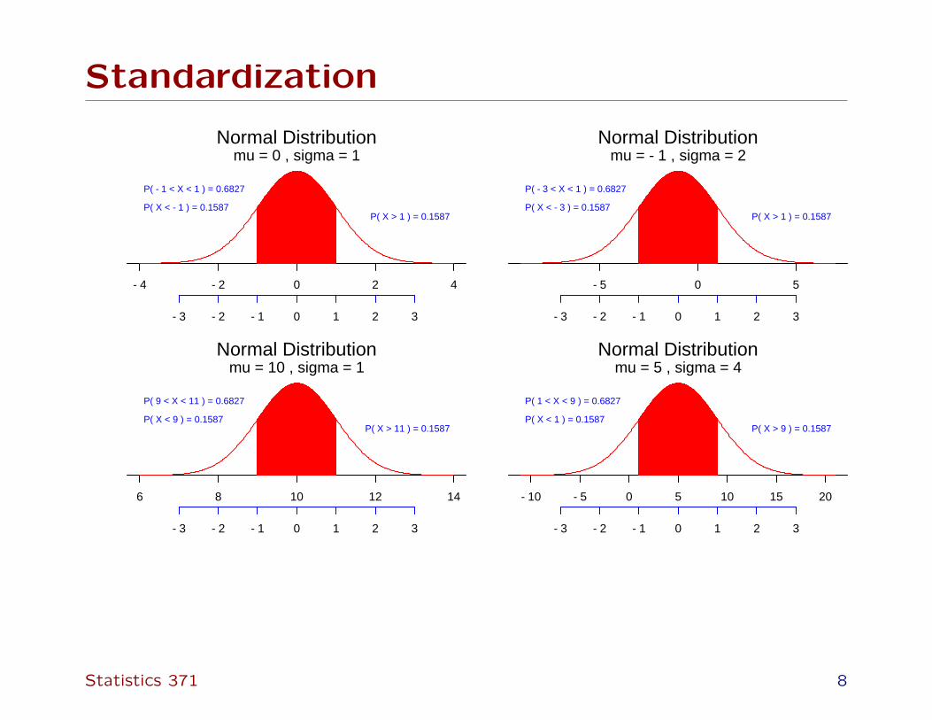
Standardization
If Y is a normally distributed Random Variable Y ∼ N(µ, σ2)
And we define
Z =Y − µ
σ
Then Z is a standard normal random variable
Z ∼ N(0,1)
Every problem that asks for an area under a normal curve is
solved by first finding an equivalent problem for the standard
normal curve.
Statistics 371 7
StandardizationP
roba
bilit
y D
ensi
ty
Normal Distributionmu = 0 , sigma = 1
−4 −2 0 2 4
P( −1 < X < 1 ) = 0.6827
P( X < −1 ) = 0.1587P( X > 1 ) = 0.1587
−3 −2 −1 0 1 2 3
Pro
babi
lity
Den
sity
Normal Distributionmu = −1 , sigma = 2
−5 0 5
P( −3 < X < 1 ) = 0.6827
P( X < −3 ) = 0.1587P( X > 1 ) = 0.1587
−3 −2 −1 0 1 2 3
Pro
babi
lity
Den
sity
Normal Distributionmu = 10 , sigma = 1
6 8 10 12 14
P( 9 < X < 11 ) = 0.6827
P( X < 9 ) = 0.1587P( X > 11 ) = 0.1587
−3 −2 −1 0 1 2 3
Pro
babi
lity
Den
sity
Normal Distributionmu = 5 , sigma = 4
−10 −5 0 5 10 15 20
P( 1 < X < 9 ) = 0.6827
P( X < 1 ) = 0.1587P( X > 9 ) = 0.1587
−3 −2 −1 0 1 2 3
Statistics 371 8

Example Calculation
Suppose that egg shell thickness is normally distributed with a
mean of 0.381 mm and a standard deviation of 0.031 mm.
Find the proportion of eggs with shell thickness less than 0.34
mm.
1. We define our random variable Y = egg shell thickness.
2. We know that
Y ∼ N(0.381,0.0312)
3. We wish to know
Pr{Y < 0.34}
Statistics 371 9

Example Calculation
Here is a way to do it in R.
> source("prob.R")> gnorm(0.381, 0.031, b = 0.34)
Pro
babi
lity
Den
sity
Normal Distributionmu = 0.381 , sigma = 0.031
0.25 0.30 0.35 0.40 0.45 0.50
P( X < 0.34 ) = 0.093
P( X > 0.34 ) = 0.907
−3 −2 −1 0 1 2 3
Statistics 371 10

Example Calculation
If you don’t have R handy, the way to do this is to transform it
into a question about a standard normal distribution.
Pr{Y < 0.34} = Pr{Y − 0.381 < 0.34− 0.381}= Pr{[Y − 0.381]/0.031 < [0.34− 0.381]/0.031}= Pr{Z < −1.322}
Where Z is a standard normal random variable: Z ∼ N(0,1).
This is exactly the type probability tabulated in a standard normal
table
Statistics 371 11

Standard Normal table
• The standard normal table lists the area to the left of z under
the standard normal curve for each value from −3.49 to 3.49
by 0.01 increments.
• The normal table is on the inside front cover of your
textbook.
• Numbers in the margins represent z.
• Numbers in the middle of the table are areas to the left of z.
Statistics 371 12
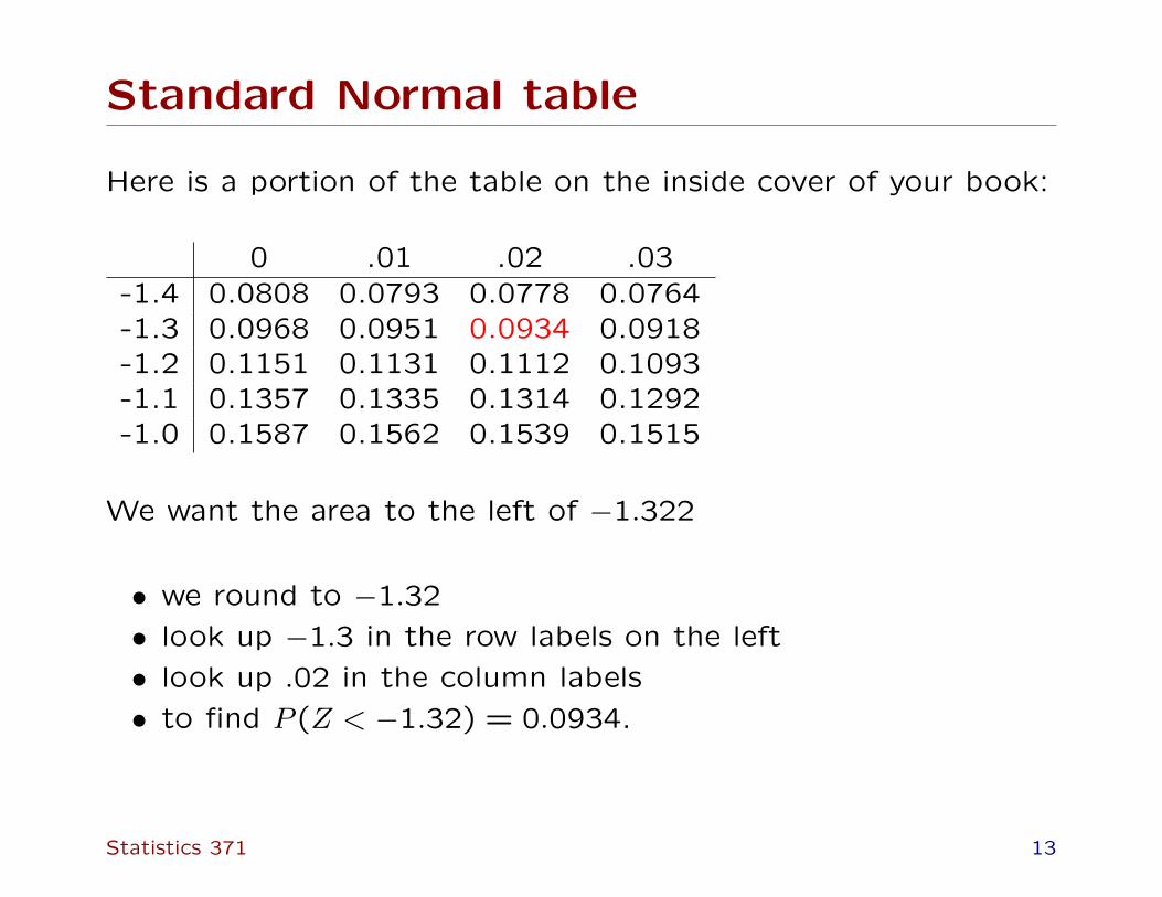
Standard Normal table
Here is a portion of the table on the inside cover of your book:
0 .01 .02 .03-1.4 0.0808 0.0793 0.0778 0.0764-1.3 0.0968 0.0951 0.0934 0.0918-1.2 0.1151 0.1131 0.1112 0.1093-1.1 0.1357 0.1335 0.1314 0.1292-1.0 0.1587 0.1562 0.1539 0.1515
We want the area to the left of −1.322
• we round to −1.32
• look up −1.3 in the row labels on the left
• look up .02 in the column labels
• to find P (Z < −1.32) = 0.0934.
Statistics 371 13

Standard Normal table
• R can do this for general values of z
• and R can do the standardization for you.
• Recall that our original question was given Y ∼ N(0.381,0.0312)what is Pr{Y < 0.34}.
Pro
babi
lity
Den
sity
Normal Distributionmu = 0 , sigma = 1
−4 −2 0 2 4
P( X < −1.322 ) = 0.0931P( X > −1.322 ) = 0.9069
z = −1.322
Pro
babi
lity
Den
sity
Normal Distributionmu = 0.381 , sigma = 0.031
0.25 0.30 0.35 0.40 0.45 0.50
P( X < 0.34 ) = 0.093P( X > 0.34 ) = 0.907
x = 0.34
Statistics 371 14

Example Area Calculations: Area to the
leftFind the proportion of eggs with shell thickness less than 0.34
mm.
> pnorm(q = 0.34, mean = 0.381, sd = 0.031)[1] 0.09298744
> gnorm(0.381, 0.031, b = 0.34, sigma.axis = F)
Pro
babi
lity
Den
sity
Normal Distributionmu = 0.381 , sigma = 0.031
0.25 0.35 0.45
P( X < 0.34 ) = 0.093P( X > 0.34 ) = 0.907
Pr{Y < 0.34} = Pr{[Y − 0.381]/0.031 < [0.34− 0.381]/0.031}= Pr{Z < −1.322} = 0.0934
Statistics 371 15

Example Area Calculations: Area to the
rightFind the proportion of eggs with shell thickness more than 0.4
mm.
> 1 - pnorm(q = 0.4, mean = 0.381, sd = 0.031)[1] 0.2699702
> gnorm(0.381, 0.031, a = 0.4, sigma.axis = F)
Pro
babi
lity
Den
sity
Normal Distributionmu = 0.381 , sigma = 0.031
0.25 0.35 0.45
P( X < 0.4 ) = 0.73P( X > 0.4 ) = 0.27
Pr{Y > 0.4} = Pr{[Y − 0.381]/0.031 > [0.4− 0.381]/0.031}= Pr{Z > 0.613} = 1− Pr{Z < 0.613} = 1− 0.7291 = 0.2709
Statistics 371 16

Example Area Calculations: Area
between two values.Find the proportion of eggs with shell thickness between 0.34
and 0.4 mm.
> gnorm(0.381, 0.031, a = 0.34, b = 0.4)
Pro
babi
lity
Den
sity
Normal Distributionmu = 0.381 , sigma = 0.031
0.25 0.30 0.35 0.40 0.45 0.50
P( 0.34 < X < 0.4 ) = 0.637
P( X < 0.34 ) = 0.093
P( X > 0.4 ) = 0.27
−3 −2 −1 0 1 2 3
Statistics 371 17

Example Area Calculations: Area
outside two values.Find the proportion of eggs with shell thickness smaller than 0.32
mm or greater than 0.40 mm.
> gnorm(0.381, 0.031, a = 0.32, b = 0.4)
Pro
babi
lity
Den
sity
Normal Distributionmu = 0.381 , sigma = 0.031
0.25 0.30 0.35 0.40 0.45 0.50
P( 0.32 < X < 0.4 ) = 0.7055
P( X < 0.32 ) = 0.0245
P( X > 0.4 ) = 0.27
−3 −2 −1 0 1 2 3
Statistics 371 18

Example Area Calculations: Central
area.Find the proportion of eggs with shell thickness within 0.05 mm
of the mean.
> gnorm(0.381, 0.031, a = 0.381 - 0.05, b = 0.381 + 0.05)
Pro
babi
lity
Den
sity
Normal Distributionmu = 0.381 , sigma = 0.031
0.25 0.30 0.35 0.40 0.45 0.50
P( 0.331 < X < 0.431 ) = 0.8932
P( X < 0.331 ) = 0.0534
P( X > 0.431 ) = 0.0534
−3 −2 −1 0 1 2 3
Statistics 371 19

Example Area Calculations: Two-tail
area.Two-tail area. Find the proportion of eggs with shell thickness
more than 0.07 mm from the mean.
> gnorm(0.381, 0.031, a = 0.381 - 0.07, b = 0.381 + 0.07)
Pro
babi
lity
Den
sity
Normal Distributionmu = 0.381 , sigma = 0.031
0.25 0.30 0.35 0.40 0.45 0.50
P( 0.311 < X < 0.451 ) = 0.9761
P( X < 0.311 ) = 0.012
P( X > 0.451 ) = 0.012
−3 −2 −1 0 1 2 3
Statistics 371 20

Using R
We have seen how to use R and the new function gnorm
to graph normal distributions where the graphs include some
probability calculations. You can also make the same calculations
without graphs using the function pnorm (the “p” stands for
probability). The following lists the commands for all of the
previous computations.
Area to the left. Find the proportion of eggs with shell
thickness less than 0.34 mm.
> pnorm(0.34, 0.381, 0.031)[1] 0.09298744
Area to the right. Find the proportion of eggs with shell
thickness more than 0.36 mm.
> 1 - pnorm(0.36, 0.381, 0.031)[1] 0.75093
Statistics 371 21

Using R
Area between two values. Find the proportion of eggs withshell thickness between 0.34 and 0.36 mm.
> pnorm(0.36, 0.381, 0.031) - pnorm(0.34, 0.381, 0.031)[1] 0.1560825
Area outside two values. Find the proportion of eggs withshell thickness smaller than 0.32 mm or greater than 0.40 mm.
> pnorm(0.32, 0.381, 0.031) + 1 - pnorm(0.4, 0.381, 0.031)[1] 0.2945190
Central area. Find the proportion of eggs with shell thicknesswithin 0.05 mm of the mean.
> 1 - 2 * pnorm(0.381 - 0.05, 0.381, 0.031)[1] 0.8932345
Two-tail area. Find the proportion of eggs with shell thicknessmore than 0.07 mm from the mean.
> 2 * pnorm(0.381 - 0.07, 0.381, 0.031)[1] 0.02394164
Statistics 371 21

Quantiles
Quantile calculations ask you to use the normal table backwards.
You know the area but need to find the point or points on the
horizontal axis.
Statistics 371 22

Example Quantile Calculations
Percentile. What is the 90th percentile of the egg shell
thickness distribution?
> source("prob.R")> gnorm(0.381, 0.031, quantile = 0.9)
Pro
babi
lity
Den
sity
Normal Distributionmu = 0.381 , sigma = 0.031
0.25 0.30 0.35 0.40 0.45 0.50
z = 1.28
P( X < 0.4207 ) = 0.9
−3 −2 −1 0 1 2 3
Statistics 371 23

Example Quantile Calculations
Upper cut-off point. What value cuts off the top 15% of egg
shell thicknesses?
> gnorm(0.381, 0.031, quantile = 0.85)
Pro
babi
lity
Den
sity
Normal Distributionmu = 0.381 , sigma = 0.031
0.25 0.30 0.35 0.40 0.45 0.50
z = 1.04
P( X < 0.4131 ) = 0.85
−3 −2 −1 0 1 2 3
Statistics 371 23
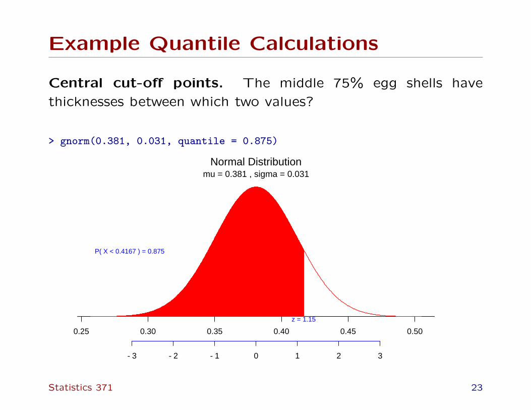
Example Quantile Calculations
Central cut-off points. The middle 75% egg shells have
thicknesses between which two values?
> gnorm(0.381, 0.031, quantile = 0.875)
Pro
babi
lity
Den
sity
Normal Distributionmu = 0.381 , sigma = 0.031
0.25 0.30 0.35 0.40 0.45 0.50
z = 1.15
P( X < 0.4167 ) = 0.875
−3 −2 −1 0 1 2 3
Statistics 371 23

Using R
You can also make the same calculations without graphs usingthe function qnorm (the “q” stands for quantile). The followinglists the commands for all of the previous computations.
Percentile. What is the 90th percentile of the egg shellthickness distribution?
> qnorm(0.9, 0.381, 0.031)[1] 0.4207281
Upper cut-off point. What value cuts off the top 15% of eggshell thicknesses?
> qnorm(0.85, 0.381, 0.031)[1] 0.4131294
Central cut-off points. The middle 75% egg shells havethicknesses between which two values?
> qnorm(c(0.25/2, 1 - 0.25/2), 0.381, 0.031)[1] 0.3453392 0.4166608
Statistics 371 24

Approximation of Discrete distributions
using the Normal distribution• The normal distribution can also be used to compute
approximate probabilities of discrete distributions.
• Approximations to the binomial distribution use a normal
curve with µ = np and σ =√
np(1− p).
• Approximations to the Poisson distribution use a normal
curve with µ = µ and σ =√
µ.
• When approximating a binomial probability, the approxima-
tion is usually pretty good when np > 24 and n(1− p) > 24.
• We will not be using the continuity correction described in
your book.
Statistics 371 25

Binomial Distributions: increasing n
0.0 0.5 1.0 1.5 2.0
0.0
0.1
0.2
0.3
0.4
0.5
0.6
Binomial Distribution n = 2 , p = 0.2
Possible Values
Pro
babi
lity
0 1 2 3 4 5
0.0
0.1
0.2
0.3
0.4
Binomial Distribution n = 5 , p = 0.2
Possible Values
Pro
babi
lity
0 2 4 6 8 10
0.00
0.10
0.20
0.30
Binomial Distribution n = 10 , p = 0.2
Possible Values
Pro
babi
lity
0 2 4 6 8
0.00
0.05
0.10
0.15
0.20
0.25
Binomial Distribution n = 15 , p = 0.2
Possible Values
Pro
babi
lity
0 5 10 15
0.00
0.05
0.10
0.15
Binomial Distribution n = 30 , p = 0.2
Possible Values
Pro
babi
lity
0 5 10 15 20
0.00
0.04
0.08
0.12
Binomial Distribution n = 50 , p = 0.2
Possible Values
Pro
babi
lity
Statistics 371 26
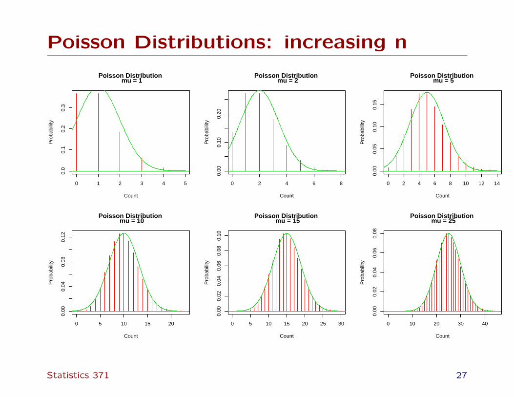
Poisson Distributions: increasing n
0 1 2 3 4 5
0.0
0.1
0.2
0.3
Poisson Distribution mu = 1
Count
Pro
babi
lity
0 2 4 6 8
0.00
0.10
0.20
Poisson Distribution mu = 2
Count
Pro
babi
lity
0 2 4 6 8 10 12 14
0.00
0.05
0.10
0.15
Poisson Distribution mu = 5
Count
Pro
babi
lity
0 5 10 15 20
0.00
0.04
0.08
0.12
Poisson Distribution mu = 10
Count
Pro
babi
lity
0 5 10 15 20 25 30
0.00
0.02
0.04
0.06
0.08
0.10
Poisson Distribution mu = 15
Count
Pro
babi
lity
0 10 20 30 40
0.00
0.02
0.04
0.06
0.08
Poisson Distribution mu = 25
Count
Pro
babi
lity
Statistics 371 27
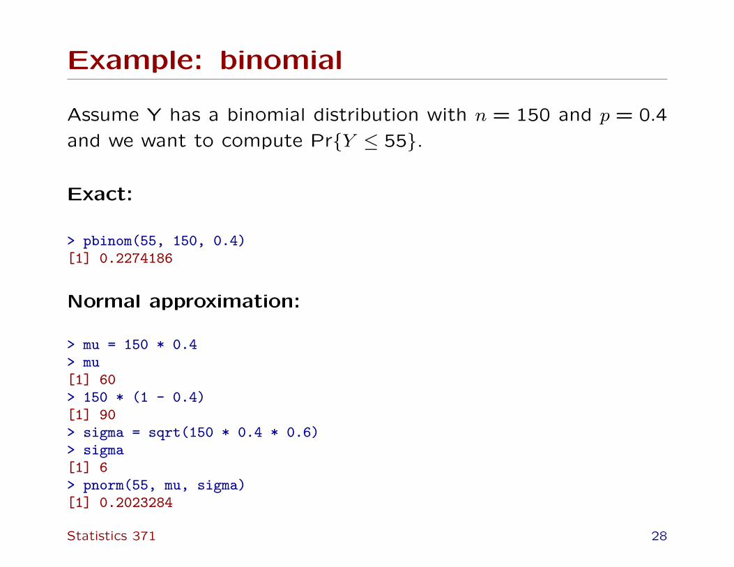
Example: binomial
Assume Y has a binomial distribution with n = 150 and p = 0.4
and we want to compute Pr{Y ≤ 55}.
Exact:
> pbinom(55, 150, 0.4)[1] 0.2274186
Normal approximation:
> mu = 150 * 0.4> mu[1] 60> 150 * (1 - 0.4)[1] 90> sigma = sqrt(150 * 0.4 * 0.6)> sigma[1] 6> pnorm(55, mu, sigma)[1] 0.2023284
Statistics 371 28

Example: Poisson
If Y has a Poisson distribution with µ = 25 what is the probability
that Y is greater than or equal to 16?
Exact:
> 1 - ppois(15, 25)[1] 0.977707
Normal approximation:
> mu = 25> sigma = sqrt(25)> sigma[1] 5> 1 - pnorm(15, mu, sigma)[1] 0.9772499
With R, do the exact calculation. With a calculator or normal
table, use the normal approximation.
Statistics 371 29