The Nonequilibrium Thermodynamics of

Radiation Interaction

Christopher EssexDepartment of Applied Mathematics

University of Western OntarioLondon, Ontario, Canada N6A 5B7

essex@uwo.ca

Dallas C. KennedyThe MathWorks, Inc., 3 Apple Hill Drive

Natick, Massachusetts USA 01760dkennedy@mathworks.com

Sidney A. BludmanDepartment of Physics

University of PennsylvaniaPhiladelphia, Pennsylvania USA 19104

andDeutsches Elektron Synchrotron

Notkestrasse 85, D-22603 Hamburg, Germanybludman@mail.desy.de

March 15, 2004

Abstract

We review some important recent developments in the nonequilibrium thermo-dynamics of radiation and matter-radiation mixtures. These include variationalprinciples for nonequilibrium steady states of photons, neutrinos, and matter inlocal thermodynamic equilibrium. These variational principles can be extendedto include mass and chemical potential. The general nature of radiation entropy,entropy production, equilibrium, and nonequilibrium is also discussed.

PACS numbers: 05.30.-d, 05.70.Ln, 11.10.Wx, 44.05.+e, 44.40.+a

Invited contribution toVariational and Extremum Principles in Macroscopic Systems,

H. Farkas and S. Sieniutycz, eds.,Amsterdam: Elsevier Science, 2004

1 Introduction

This review presents recent results in the nonequilibrium thermodynamics of ra-diation. The term “radiation” means nothing more than particles moving alonga ray [1]. It is broad enough to include massless, nonconserved quanta of anytype – photons but also neutrinos, for example. The fundamental point of theinvestigations described here is to develop a framework for the nonequilibriumthermodynamics of systems composed of any particles. Elementary particlesare the quanta of quantum fields, the fundamental entities of physics [2, 3]. Ageneral thermodynamics based on quantum fields would be difficult and notilluminating. A middle ground between a quantum field and a macroscopicdescription is more useful [4]. In practice, a quantum field description can bereduced to a description in terms of quanta of field modes. The modes arelabeled by position, momentum or wavenumber, and possibly other quantumnumbers such as spin (polarization, in classical terms), charges (electric, bary-onic, leptonic, etc.), or particle identity. The space of all these labels is modespace; position and momentum alone define phase space.

A broad feature of this picture of thermodynamics emerges from the practi-cal distinction between “matter” made of massive, conserved quanta (electrons,neutrons, protons, etc.) and massless or nearly-massless “radiation” such asphotons and neutrinos [5, 6]. In most situations, matter is localizable in spaceand naturally forms “blobs.” The momentum of microscopic particles can behidden by partial integration of phase space, leaving only position space. Mat-ter thermodynamics is then formulated in terms of static functions over finitevolumes. In contrast, except in exotic conditions such as stellar interiors, radi-ation is usually “free-streaming,” in constant motion and not localized. Radi-ation usually requires an explicit description of momentum as well as positionspace, so that the natural extensive functions are fluxes representing beams, not“blobs” [7, 8]. This picture is familiar from everyday life: matter is localizedand close to equilibrium; radiation is out of equilibrium and not localized. It isstreaming photon beams that inform us about the localized matter blobs.

These conditions reflect a distinction familiar in the physical world. Mas-sive, conserved matter and normally hidden short-range forces (interatomic,intermolecular, weak and strong nuclear forces) are localized in space. Masslessparticles (photons, neutrinos, gravitons) generate long-range effects that can benaturally viewed as nonlocal. But if we take into account momentum as wellas position variables, the physics of massless quanta is just as local as that ofmassive particles. Classical thermodynamics, for historical reasons, often biasesour thinking with localized matter as the sole paradigm [9, 6]. All particlesare in motion in any case, but radiation makes this fact inescapable. Classicalthermodynamics also bends our thinking towards macroscopic or phenomeno-logical descriptions, at least for matter. But the mode space of quantum fieldsprovides a single comprehensive framework for expressing the degrees of free-dom of all particles, bosons or fermions, massive or massless, conserved or notconserved [10].

1

1.1 Entropy Without Equilibrium

After counting the quanta of field modes, physical quantities – energy, volume,entropy – can be constructed for the fields, mode by mode [9]. If the modeentropy is a function of other mode variables such as energy, we can even deriveintensive thermodynamic variables – such as temperature – mode by mode [11,12]. These differ for each mode, unless the system in question is in equilibrium.What results is a generalization of classical nonequilibrium thermodynamicsto the full mode space. As long as the list of mode labels is complete, thethermodynamics is also complete. Section 2 gives some examples of constructingthe entropy for massless quanta independently of equilibrium. The method canbe used for the quanta of any field.

1.2 Entropy Production in Volumes and on Surfaces

A thermodynamic system out of equilibrium exhibits differences of intensiveparameters αa, as well as the creation, flow, and destruction of extensive vari-ables Ha. For example, temperature differences drive heat flows, and pressuredifferences drive volume flows. Differences in intensive variables αa, conjugatein the entropy picture to Ha, are thermodynamic forces Xa = ∆αa; the flowsare thermodynamic fluxes Ja. The local definition of variable intensive parame-ters requires local thermodynamic equilibrium (LTE) [6, 8, 9]. The LTE conceptcan be generalized to locality not only in position space, but anywhere in modespace.

The entropy production Σ of a system can be expressed as a sum of productsof intensive differences and their associated extensive fluxes. The general Gibbsform of the entropy increment is dS =

∑a αa · dHa. The entropy production

from any intensive-extensive pair is Σa ∼ Xa · Ja ≥ 0. The value of Σ suggeststhe rate at which a system is approaching equilibrium or, if it is constrainedto avoid equilibration, how much entropy must be dissipated to keep it in thatstate. In the latter case, the outside constraints must also supply the flows ofheat, matter, etc., that maintain the nonequilibrium state.

Entropy production can be expressed as a volume integral over a nonequilib-rium system. Some forms of entropy production are strictly local, while othersarise from spatial currents. Local forms can be defined in the familiar wayusing densities of extensive variables. The current terms represent both trans-port entropy production within the volume and possibly surface contributions.If the system is in a steady state, the entropy production rate is constant. Ifthe system is in local thermodynamic equilibrium, intensive parameters are de-fined, and important simplifications become possible. Entropy production canbe expressed in macroscopic form or in terms of the statistical distributions ofquanta [6, 13, 11, 10].

An aspect of local equilibrium is that intensive forces and extensive fluxesusually have, to good approximation, a quasi-linear relationship [19]. In thisregime, fluxes, at the first order, are linear combinations of forces, with transportcoefficients that can vary across the system. These coefficients need not be

2

constant, as long as they are strictly functions of the local state and contain nogradients or nonlocal differences.1

The term nonlocal difference indicates a difference of functions of intensivethermodynamic quantities driving radiative exchanges between elements of mat-ter located at finite distances from one another. Such nonlocal differences aretypical of radiation-matter interaction and should be contrasted with the gra-dients that normally drive thermodynamic flows in matter in LTE. In general,the radiation need not be in LTE, but LTE itself can be defined in a very gen-eral way. The most general LTE requires all intensive parameters to be definedlocally in mode space. It also requires extensive parameters to be continuousover different parts of a system, a requirement automatically satisfied by variousmacroscopic conservation laws.

In the quasi-linear approximation, the volume part of the entropy productionthen becomes a sum of bilinear expressions force × flux ∼ force × transportcoefficient × force. These functions are local in mode space. Expressions strictlylocal in position space emerge as limiting cases where the momenta and othermode variables are summed over. Many such limits are possible, depending onthe nature of the system.

Surface contributions to the entropy production occur if there are sharpboundaries to the system [1, 14, 15]. In LTE, the entropy current is a linearcombination of currents of extensive variables, with the intensive parametersas coefficients. This form is analogous to the bilinear form taken by the localvolume terms. LTE again allows currents to be related in quasi-linear fashionto thermodynamic forces, usually gradients of intensive variables. On the otherhand, if the quantum statistical distributions are known, the currents can beexpressed that way instead. Radiation is simple enough that its thermodynamicproperties can be expressed exactly in terms of quantum distributions [13, 8].The simplicity of radiation thermodynamics arises from photon number non-conservation and the absence of a photon chemical potential.

Another simplification is possible if the radiation entropy production van-ishes. In that case, we can consider matter-matter interactions mediated byradiation and eliminate the radiation modes [1, 11]. In position space, radiationthen becomes a kind of nonlocal heat transport, and Σ can be represented ina multilocal form. If radiation streams in free space and interacts with mat-ter only at discrete locations, we end up with a description of localized matterlumps interacting at a distance via the field. This multilocal thermodynamicform parallels the action-at-a-distance form of electrodynamics. In both cases,the field is eliminated as a dynamical entity [16].

Under certain conditions, the radiation itself can be localized, as for examplein an opaque plasma. The diffusion of radiation then becomes a type of volume-based local transport. Radiative heat transfer in that case is formally similarto heat conduction, which is a purely local matter-matter interaction involvingno radiation.

1This condition is identical to the requirements for the validity of the first-order Chapman-Enskog method of reducing microscopic statistical kinetics to macroscopic thermohydrody-namic behavior and expressing transport coefficients in terms of statistical distributions [8].

3

Radiation is often viewed in this way, merely as a mediator and not an entityin its own right, leading at times to erroneous results. But radiation does haveits own properties and conditions independently of matter, and it is sometimesessential to account for these explicitly.

1.3 Entropy Production and Minimum Principles

Besides characterizing a nonequilibrium system’s state, the entropy productionfunction has a dynamical significance under certain conditions [5, 17, 18, 6, 19,9]. Expressed as a function of thermodynamic forces or of local intensive vari-ables, the entropy production is a minimum in a nonequilibrium steady state(NESS), subject the external constraints that prevent the system from equi-librating. The most familiar form of this variational principle is the classicalmacroscopic nonequilibrium thermodynamics of matter systems, where the en-tropy production can be expressed as a quadratic function of thermodynamicforces. The principle holds in the local quasi-linear case, where the thermody-namic forces are subject to variations, but the background transport coefficientsare not.

Less familiar but equally important are surface contributions, of which radia-tion is simplest and most common. The minimum entropy production principleholds with these terms included. For radiation, the entropy production is asimple function of local temperature and requires no approximations [13, 1, 11].

2 Entropy With and Without Equilibrium

What makes thermodynamic systems nondeterministic is the statistical uncer-tainty associated with microscopic states. A thermodynamic system can beviewed as an ensemble of many copies of the same physical system, each differ-ent from the others in microscopic details, but all sharing the same macroscopicexpected values of volume, energy, and so on. A measure of the statistical un-certainty of microscopic details is the macroscopic entropy S, a nonnegativefunction of the ensemble’s statistical ensemble [9, 6].

A thermodynamic ensemble of zero entropy contains only one, completelydetermined, system copy. With multiple copies, the entropy is positive. Eachmicroscopic configuration has its own probability pk. The entropy of a thermo-dynamic system is a sum over all possibilities k :

S = −kB

∑

k

pk ln pk , (1)

subject to the constraint∑

k pk = 1. In the completely determined case, all pk

= 0 except for one possibility j, pj = 1. In that case, S = 0.All system variables, such as volume, energy, and entropy, are defined for a

thermodynamic system whether that system is in equilibrium or not. In general,however, computing S requires knowing the probabilities pk of all microscopicpossibilities.

4

Comment: So that S be additive, a logarithm of any basis is acceptable.The natural log is the simplest choice. Changing the log basis multiplies Sby an overall constant. The standard thermodynamic entropy also contains anadditional factor of Boltzmann’s constant kB . If the entropy is computed usingthe system’s fundamental degrees of freedom, entropy is fully defined withoutany free constants.

2.1 The Case of Equilibrium

Entropy is maximal in equilibrium, typically under the constraint of holdingfixed certain macroscopic state variables such as energy or number [9]. In equi-librium, S is a function of these other macroscopic variables. For each mi-croscopic configuration k, a system variable Ha has a value Ha

k . A Lagrangemultiplier αa is associated with each system variable average 〈Ha〉 =

∑k pkHa

k

held fixed for maximal entropy. Then maximizing S under constraints is equiv-alent to maximizing

S −∑

a

αa〈Ha〉 − α0

∑

k

pk = −kB

∑

k

pk ln pk −∑

ak

αaHak − α0

∑

k

pk .

The resulting probability distribution is

pk =exp[−∑

a αaHak ]∑

j exp[−∑a αaHa

j ], (2)

the generalized Boltzmann distribution. The denominator of (2) is the system’spartition function. Each αa is the intensive variable conjugate to its correspond-ing extensive variable Ha. For example, if H is the energy E, then α = 1/T,where T is the temperature.

Consider a system of nonconserved, massless elementary quanta in thermalequilibrium [11, 4]. The system can be analyzed in terms of the phase spacelabels position r and momentum p of a single particle. The energy ε of a singlequantum is c|p| = hν. The mean occupation number of mode p is a functionof x = hν/kBT :

np =1

ex ± 1. (3)

The ± sign holds for fermions (bosons). (See section 2.2 below.) The energy inthe differential phase volume d3r d3p is

2(kBT )4

(hc)3x3

(ex ± 1)dx dΩp d3r , (4)

where Ωp is the solid angle in momentum space. (The factor of two which countstwo radiation polarization states may be dropped, but we keep it to match theconventional definition of radiation flux.) When the integration over x is carriedout, the fourth-power dependence of energy on T follows for both bosons and

5

fermions. The only difference between the two is in the numerical factor of theintegral due to the “±” in the denominator in the integrand of the x integration.The analogous infinitesimal contribution to the entropy from a differential phasevolume is

2kB(kBT )3

(hc)3[ x3

(ex ± 1)± x2 ln(1± e−x)

]dx dΩp d3r . (5)

This implies the standard equilibrium third-power dependence of entropy ontemperature, for fermions and bosons.

The four integrals:∫ ∞

0

x3

(ex ± 1)dx =

15∓ 116

(π4

15

), (6)

and∫ ∞

0

±x2 ln(1± e−x) dx =15∓ 1

16

(13

)(π4

15

), (7)

are easily deduced by series expansions. The Stefan-Boltzmann radiation con-stant is σ = 2π5k4

B/15h3c2. From these we find the energy per unit volume intosolid angle dΩp,

15∓ 116

( σ

πc

)T 4dΩp . (8)

Similarly for the entropy,(4

3

)15∓ 116

( σ

πc

)T 3dΩp . (9)

The vector flux density of energy into solid angle dΩp with direction p is

15∓ 116

(σ

π

)T 4 p dΩp , (10)

and for entropy,(4

3

)15∓ 116

(σ

π

)T 3p dΩp . (11)

The integrals (6-7) give the canonical fermion factor of 7/8 relative to bosons.The flux density per solid angle, also known as the specific intensity or radiance,is for energy,

15∓ 116

(σ

π

)T 4 , (12)

and for entropy,(4

3

)15∓ 116

(σ

π

)T 3 . (13)

6

These results for surface emission of nonconserved quanta can be extendedto massive particles. (Some or all of the neutrino species, in fact, have smallmasses [20].) With nonzero mass, the momentum integrals cannot be evalu-ated in closed form, but they can be easily calculated numerically. Define themomentum integrals with nonzero mass as:

(15∓ 116

)(π4

15

)·g1

f1

(m) ≡

∫ ∞

0

x3 dx

e√

x2+m2 ± 113

(15∓ 116

)(π4

15

)·g0

f0

(m) ≡

∫ ∞

0

(±x2) ln(1± e−√

x2+m2) dx (14)

with the upper sign for fermions and the lower for bosons. The new f andg functions are defined such that fi(0) = gi(0) = 1. The reduced mass mincorporates the temperature: m ≡ mc2/kBT .

The specific energy and entropy flux expressions change their forms to:(15∓ 1

16

)g1

f1

( σ

cπ

)T 4 ,

(15∓ 116

)g0/3 + g1

f0/3 + f1

( σ

cπ

)T 3 . (15)

The overall fourth- and third-power dependence on temperature for the energyand entropy fluxes remains. But these expressions contain additional depen-dence on T through m. Differentiation of these expressions with respect to Trequires varying this additional dependence as well as the overall power depen-dence.

2.2 Entropy Without Equilibrium: Counting Quanta

The microscopic probabilities pk cannot be determined, in general, without adescription of the statistical ensemble in terms of its degrees of freedom andhow it was created. In some cases, however, and without equilibrium, simplecounting arguments are enough to define a system’s thermodynamics, by findingS as a function of other state variables such as E and N . It is even possible todefine subsystem intensive variables such as temperature under certain restric-tions [12].

Elementary bosons or fermions provide a simple example. These quantacan be, for example, photons or neutrinos, although they need not be massless.Elementary particles are the quanta of quantum fields, and the fundamentaldegrees of freedom are the modes of these fields. The description of the state of abosonic field must also include the amplitude and phase (as well as polarization,etc., where necessary) of each mode. A quantum state of complex amplitudeand other mode labels is a coherent state [2].

For fermions, the amplitude and phase are trivial, because of the Pauli ex-clusion principle: a fermionic field mode can have at most one quantum. Thereare no fermionic coherent states. For bosons, the amplitude and phase can beanything. A bosonic mode can have any number of quanta.

7

For fermions and for boson fields with random mode phases, a special sim-plification is possible. The state of the quantum field becomes equivalent tocounting the number of quanta in each mode. Calculating the entropy of themode is then straightforward, a generalization of the counting familiar fromequilibrium quantum statistical mechanics.

Consider an ensemble of M identical systems. Each system has the sameinternal probabilities for being in any particular state k, pk. The number ofsystems in state k is M · pk = mk. Suppose that the collection of systems havem1 systems in state 1 and m2 systems in state 2, etc. The number of ways thatthis configuration can happen is

WM = M !/[m1!m2!...mk!...] .

The entropy is

S = −kB

∑

k

pk ln pk .

This expression is equivalent to

SM = kB ln WM ,

if we use probability normalization∑

k pk = 1, the definition of mk, and Stir-ling’s formula n! ∼√2πn nne−n, for large n. (Stirling’s formula is quite accurateeven for n ∼ 10.)

Now compute W for bosons and fermions. Consider N identical quanta andG identical possible “places” to put them.

• With no constraints on N, the boson case, there are WB = (N + G −1)!/[N !(G− 1)!] ways of arranging the N quanta among the G places.

• With the constraint that no more than one quantum be permitted in eachof the G places, the case of fermions, there are WF = G!/[N !(G − N)!]ways of arranging the N quanta among the G places.

Use Stirling’s formula again to simplify the expressions for S in the two cases,and define a mean occupation number n ≡ N/G. Then the entropy for thebosonic and fermionic cases is:

S = ±kB · (1± n) ln(1± n)− kB · n ln n , (16)

with the upper sign for bosons and the lower for fermions.Although equilibrium is not assumed, the expression for S looks formally

like the expression for S in equilibrium, and it is independent of any assump-tion about the nature of the ensemble, apart from the random mode phaseassumption. This expression for S applies to a single mode of the field. Themode has n quanta. The entropy for many modes is just the sum of the en-tropy for each mode. This derivation assumes that the number of quanta can

8

be counted, but that N is not conserved. Thus no chemical potential entersinto the thermodynamic description. The entropy S is plotted as a function ofn in Figure 1. In the boson case, n must be nonnegative. In the fermion case,0 ≤ n ≤ 1.

The energy per quantum is ε ≡ hν. A natural temperature for a single modefollows:

hν

kBT=

∂S

∂n= ln

( 1n± 1

). (17)

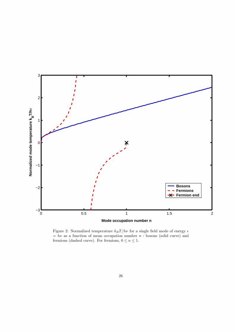
Here, T is a subsystem temperature, and in the case of photon modes, oftencalled the brightness temperature [7, 8]. The expression (17) looks like thetemperature one would infer by inverting the usual Bose-Einstein or Fermi-Dirac equilibrium distributions. In this analysis, however, n is arbitrary, and Tis different for each mode in general. The function kBT/hν is plotted in Figure 2as a function of n. The fermionic mode temperature is negative for 1/2 < n< 1.

2.3 Entropy Without Equilibrium: Fluxes

For closed systems, the thermodynamics can be expressed in terms of extensivevariables and their densities. But in general, we consider open nonequilibriumsystems with flows and avoid confining the system to a box. Also, if the quantaare massless, they cannot be brought to rest. Using densities is clumsy, and itis better to use fluxes as the primary extensive quantities [1, 15, 10].

With or without equilibrium, we can relate the specific energy intensity Ip,for a given p, to the mode occupation number np from equations (8) and (10)and the flux density into a solid angle,

Ip =2npε3

h3c2. (18)

The specific entropy intensity Jp is

Jp =2kBε2

h3c2

[∓

(1∓ c2h3Ip

2ε3

)ln

(1∓ c2h3Ip

2ε3

)−

(c2h3Ip2ε3

)ln

(c2h3Ip2ε3

)]. (19)

The fundamental extensive quantities are the specific entropy and energy fluxJp and specific energy flux Ip. Note that expression (17) for the temperatureTp is recovered by forming dJp/dIp.

In the case of photons, number is not interesting, as photon number isnot conserved. In the case of fermions, some number conservation law usu-ally holds [3]. With zero chemical potential, however, the fermion number is apurely auxiliary quantity and depends on the energy flux. Conversely, we couldtake fermion number as fundamental and energy as derived; in either case, onlyone variable is independent. In the case of nonzero chemical potential, fermionnumber and energy flux become independent variables, with a mode-dependentchemical potential µp.

9

Since neutrino number is not conserved but lepton number is, it is importantto define a specific number flux for neutrinos Np corresponding to Ip:

Np =2npε2ph3c2

, (20)

where Ip = εpNp.

2.4 Entropy Without Equilibrium: Quantum Fields

For quantum systems, an equivalent ensemble description uses the density oper-ator ρ. It is Hermitian, and its real eigenvalues are the microscopic probabilitiespk, satisfying Tr(ρ) =

∑k pk = 1. The entropy S = −kBTr(ρ ln ρ). A com-

pletely determined system is in a pure state: one pj = 1, the other pk = 0. Inthis case, the entropy vanishes, and the density operator satisfies ρ2 = ρ and canbe expressed as ρ = |ψ〉〈ψ|, where |ψ〉 is some quantum state. In the nontrivialcase, S > 0, 0 ≤ pk < 1, and ρ2 < ρ (in the spectral sense) [9, 4].

For fermions, the Pauli exclusion principle keeps the entropy simple. With-out fermionic coherent states, the problem of computing entropy for fermionicfields reduces back to counting quanta. But without random mode phases,computing the entropy of a bosonic field becomes problematic.

For bosons, a general ensemble is a composite expanded over a basis ofprojection operators. The basis can be the occupation number basis or the co-herent state basis, for example. The ensemble is described by a density operatorρ expanded over some basis ψ :

ρ =∫

d[ψ] d[ψ′] P (ψ, ψ′) |ψ〉〈ψ′| .

Because ρ is Hermitian, P is real.Unfortunately, a general bosonic field ensemble ρ is very difficult to analyze

and diagonalize. Only two special cases seem to be tractable: random modephases and the pure state. Equilibrium is a subcase of the random mode phasecase [12].

3 Entropy Generation and Variational Princi-ples

A thermodynamic system out of equilibrium has currents transporting heat, par-ticle number, volume, etc., from one region of mode space to another. Externalconstraints holds the system out of equilibrium, and a nonequilibrium systemis necessarily open. Quantities not locally conserved in microscopic interactions(such as collisions and matter-radiation couplings) relax in some characteristicequilibration time(s) to a local equilibrium, leaving only locally conserved quan-tities Ha not in local equilibrium.2 (Because it is conserved, each Ha retains

2The other set of macroscopic variables that does not relax towards equilibrium are orderparameters arising from broken symmetries, usually associated with phase transitions.

10

memory of its initial value and thus does not move towards equilibrium.) Toeach of these conserved Ha is associated a nonzero flux Ja and a conservationlaw, such as an equation of continuity for densities and currents. The nonzerofluxes Ja are maintained by boundary conditions. Thermodynamic “flux” refersto spatial currents and local creation rate densities alike [21, 17, 5, 6, 9].

If the microscopic equilibration acts over short enough times and smallenough spaces, each Ha also has an associated intensive parameter αa. Thisintensive parameter is constant over the system if and only if the associated fluxJa is zero, defining a global equilibrium for that particular Ha. Otherwise, theαa varies in space and time. LTE implies that whatever space and time scalesare necessary for local equilibration to occur, they must be much smaller thanthe intensive scale heights |αa/∇αa| and scale times |αa/αa|.

In a nonequilibrium steady state, the system’s intensive parameters and den-sities and fluxes of extensive parameters do not vary in time. The macroscopicconservation laws then reduce to zero-divergence conditions on the associatedcurrents. If the system is not steady, then the full conservation laws hold, re-quiring time derivatives as well as divergences in the equations of continuity.

The entropy production associated with each nonequilibrium current Ja andassociated force Xa arises from the Gibbs form of the entropy differential dS=

∑a αa · dHa. The thermodynamic force Xa can be, for example, a spa-

tial gradient of an intensive parameter, the infinitesimal change of αa over aninfinitesimal distance. Or it can be a finite difference of chemical potentialsbetween reagents and products. We must account for the entropy both gainedand lost from nonequilibrium flows and impose the condition that each Ha beconserved (Ja

out = −Jaout). Then the entropy production rate always has the

form

Σ =∑

a

(αina Ja

in + αouta Ja

out) =∑

a

(αina Ja

in − αouta Ja

in) =∑

a

Xa · Ja , (21)

if LTE holds for each Ha.3 The sum in general extends over all mode labels.

3.1 Forms of Entropy Production – Minimum Principles

Entropy is an extensive thermodynamic property. It can be localized and inte-grated to determine a global amount. Entropy production Σ is also extensive,localizable, and a volume integral of its local density σ. (We use σ to representthe Stefan-Boltzmann constant as well. The distinction is clear from context.) Ifwe divide space into distinct regions, boundary surfaces are defined; entropy canmove between regions, and entropy fluxes across surfaces are defined [5, 18, 6, 9].

The entropy production rate can be expressed as

σ =∂s

∂t+∇ · F ≥ 0 , (22)

3If LTE is not valid for one of the Ha, the associated entropy production has to be computedfrom the microscopic kinetic expression derived from the universal definition of entropy (1),which implies dS = −kB

∑k

dpk · ln pk.

11

where σ is the entropy production rate per unit volume, s is the volume densityof entropy, and F is the entropy flux density. This inequality expresses, indifferential form, the total entropy change within a volume and the second lawof thermodynamics.

The significance of this form of σ is that it naturally divides into two setsof terms. The first set consists of local densities which, if expressed in termsof a LTE, can be resolved into bilinear forms X · J, where the J ’s are creationrate densities. The second set consists of divergence terms. When integratedover the system volume, these can be recast as surface integrals of currents.If these fluxes are emitted from surfaces in LTE, they can be expressed asfunctions of surface intensive parameters. This separation of local densities andflux divergences is more than formal [11]. A typical system has a “matter” partmade of heavy, nonrelativistic particles and a radiative part made of massless ornearly-massless particles. Assume we can draw a boundary over a large enoughvolume to permanently contain all the matter, including matter currents andwork in the rest frame of this matter. The radiation, being massless, has no restframe and always has associated flux currents. (Nearly massless neutrinos dohave a rest frame, but it is very different from the typical rest frame of “matter.”)Only if the “matter” is virtually opaque, locally trapping the radiation, can theradiation be described in local terms. Examples of such systems are discussedin section 5.

Separating entropy production into radiative and matter parts, σ = σm +σr,

σ =∂sm

∂t+

∂sr

∂t+∇ ·Y +∇ ·H , (23)

where sm (sr) is the volume density of entropy in matter (radiation). Y and Hdenote matter and radiative entropy flux densities, respectively.

By using the equations of state and steady-state conservation equations forthe extensive variables, we re-express the matter entropy flux divergence as∇ ·Y =

∑a∇·(αaYa) and the local matter entropy production as

∑a αaεa.

(This step defines the intensive αa simultaneously in terms of extensive fluxesand volume densities.) The Ya and the εa are the flux densities and creationrates of the extensive variables Ha, respectively. The entropy production ratebecomes a sum of local matter, matter transport, and radiative terms:

σ =∑

a

αaεa + Ya·∇αa+∇ ·H , (24)

αa is the intensive variable conjugate to Ha. For a system in a steady state, theradiative entropy density is constant, and we set ∂sr/∂t = 0. In (24), the secondand third terms become surface terms when σ is integrated over a volume.

Entropy production is a minimum in a NESS of an open system in LTE,holding fixed the boundary conditions that keep the system from equilibrating.Entropy production in general includes both volume integrals of local densitiesand surface integrals of currents [13, 11, 5, 18, 6, 19].

12

3.2 Local Equilibrium and Local Entropy Production

The familiar form of entropy production and the minimum entropy productionprinciple arises from the local density terms in σ. Without further assumptions,the bilinear form X ·J is purely kinematic and says nothing about the system’sdynamics. While all X = 0 implies all J = 0, there is no general functionalrelation between forces and fluxes. Within LTE, however, the J can usuallybe expanded in powers of the X and well-approximated by linear forms, Ja

=∑

b K∗ab(α∗)Xb. If the system is described in terms of quantum statistical

distributions, we could express σ in terms of intensive parameters such as T,without expansions. But this last step is not necessary for a minimum principle.

In general, the transport coefficients Kab are not constant over the wholesystem, and the relation of the J to the X is quasi-linear [19]. (In the strict linearregime, the Kab are constant across the whole system.) Instead, the Kab dependon the local thermodynamic state, through the local intensive parameters α∗only (not their gradients or other nonlocal differences). The special ∗ subscriptdistinguishes the local αa’s from differences of intensive parameters that occurin the thermodynamic forces Xa. If the microscopic dynamics are reversible,the Kab are symmetric [17].

Two important variational principles are associated with the local bilinearentropy production [18, 19]. The distinction depends on the choice of boundaryconditions. In one case, the entropy production of an LTE-NESS systems is aminimum with respect to variation of the forces Xa, holding fixed the subsetof thermodynamic forces that keep the system from equilibrating. In the other,the entropy production is a minimum with respect to variation of all the forces,holding fixed a set of external thermodynamic fluxes that keep the system fromequilibrating. We vary the thermodynamic forces Xa formed from differences ofintensive parameters, while holding fixed the purely local intensive parametersα∗ that occur in the K∗

ab. The procedure is similar to the background field,external field, and self-consistent field methods used in statistical and quantumfield theory [22].

The first entropy production minimum principle uses the simple bilinearform, Σ =

∑ab XaK∗

abXb. Vary Σ with respect to the Xa’s that are not heldfixed by the boundary conditions. This variation, which is proportional to theassociated thermodynamic flux, vanishes. Each δX is independent, so that eachassociated thermodynamic flux is zero. Those X’s allowed to vary and theirassociated fluxes are those aspects of the system that have equilibrated. ThoseX’s held fixed and their associated fluxes are held by boundary conditions outof equilibrium.

The second entropy production minimum principle allows all the X’s tovary, but explicitly includes the external currents Jext that keep the systemfrom equilibrium. Such boundary conditions are often the realistic choice, sincereal systems are often prevented from equilibrating by external pumping, i.e.,imposed fluxes, not by imposed forces. In this principle, the internal entropyproduction has a second-order, quadratic form, because the system internallyis everywhere in LTE. (The first-order local increment of entropy must vanish.)

13

The general form is

Σ =∑

ab

12XaK∗

abXb +∑

a

Xa · Jaext . (25)

Varying all the X’s independently and setting to zero each contribution to Σyields a conservation law for each flux J .

For every nonvanishing Jaext, the corresponding internal Ja is also nonvan-

ishing. A conjugate subset of the X is nonvanishing. These parallel subsetsof nonvanishing forces and fluxes represent the nonequilibrium aspect of thesystem.

3.3 Streaming Fluxes and Radiative Entropy Production

The radiative and matter entropy flux parts of Σ can be expressed as a surfaceintegral through the divergence theorem.

Σsurface =∫

V

dV ∇ ·H +∑

a

Ya·∇αa =∫

S

dS · H +∑

a

αaYa . (26)

There is a constant entropy production from the release of radiation into emptyspace. This step requires the radiation to propagate freely from a well-definedsurface. Any flow of extensive matter quantities Ha across the surface alsocontributes to the entropy production [13, 1, 14, 15, 6, 9].

For example, the local photon entropy flux H has magnitude (4/3)σT 3eff on

a surface with temperature Teff . Multiplying this expression by the surface areagives the total boundary entropy production, Σbound. In fact, the boundaryexpression is simply the total Σrad within the enclosed volume, including allentropy production due to radiation production and transport. The volumeintegral of σ is the entropy production up to, but not including, the surface; thesurface integral or boundary term is the photon entropy production includingthe surface, as well as the interior. Thus, the contribution of the surface aloneto Σrad is the difference of these two expressions: Σsurface = Σbound− Σvolume.

4 Free Radiation and Equilibrium Matter

Radiation produces entropy only when it interacts with matter. If matter andradiation are separated, the two can interact only at boundaries. The radiationfield is composed of absorbed and emitted parts. If the matter is isolated intolumps each in LTE, each lump has a temperature that can vary over its surface.The lump emits locally as a black body. The absorbed field can have its owntemperature independent of the matter thermodynamics, while the emitted fieldshares the same temperature as the matter at the point of emission. If tem-perature varies within the body, then nonequilibrium matter thermodynamicsis the correct framework for that part of the problem [13, 1, 11].

14

Separation of forces and fluxes is superfluous for radiation, which we treatexactly in terms of temperature. We do not count elementary quanta for matter,on the other hand, and the associated entropy production must still be computedas heat flux divided by temperature and in quasi-linear form. In this section,we use intensive variables to study radiation and radiation-matter coupling andtreat extensive variables and fluxes as secondary. This treatment agrees withthe first-order variational approach.

Entropy production provides a variational principle for systems consisting ofdiscrete lumps of matter emitting radiation freely into empty space. The detailsof the respective distributions for bosons and fermions differ, but the generalform of Σ and the principle of minimum entropy production holds [11].

4.1 Entropy Production at Matter-Radiation Boundaries

If we integrate over a finite volume V bounded by a surface S containing all thematter, then the entropy production rate Σ is

Σ =∫

V

∑

k

akεk dV +∫

S

H · dS , (27)

because matter fluxes must vanish across S.Terms under the first integral of (27) are all due to matter processes and

not part of the radiative entropy production. It is a common misconception tointerpret the radiation heating rate divided by the temperature, which occursin the first integral, as the entropy production of radiation. It should be clearfrom this derivation that

∫V

σrad dV is all accounted for through the secondintegral of (27).

Equation (27) is the basis for computing the entropy production rate dueto the interaction of matter and radiation for many finite bodies locally inequilibrium. The first term represents changes in the entropy of the bodieswhile the second term accounts for changes in the radiation field.

Separate the energy and entropy fluxes into incoming and emitted compo-nents: F = Fi + Fe, H = Hi + He. The emitted components are assumed tobe thermal, Fe = σT 4m and He = (4/3)σT 3m, respectively, where m is theoutward unit vector normal to the body surface. If photon radiation is incomingon a body of temperature T in a vacuum, the entropy production rate is

Σγ =∫

V

(−∇ · F

T

)dV +

∫

S

H · dS , (28)

where the volume V is any containing the body, and F is the flux densityof energy radiation. Next the divergence theorem is used. The temperaturegradient terms vanish because the gradients are defined only inside S, while theradiative fluxes are defined at and outside S.

Σγ = −∫

S

F · dST

+∫

S

H · dS . (29)

15

Restate the result using the blackbody expressions:

Σγ =∣∣∣∣∫

Fi · dST

∣∣∣∣−∣∣∣∣∫

Hi · dS∣∣∣∣−

∫σT 3dS +

∫(4/3)σT 3dS . (30)

The incoming flow is independent of the state of the body. Thus it follows that

δΣγ =∫ [

σT 4 − Fi · m] δT · dS

T 2= 0 , (31)

since Hi is independent of T . Since the variation δT is arbitrary, the integrandmust also vanish. That is, the entropy production rate is a minimum in thesteady state, implying energy conservation, for an arbitrary geometry and in-coming field. This is an example of a conservation law derived from minimumentropy production [1, 15, 11].

4.2 Example: Free Radiation and Matter Lumps

Now consider a thermalized and isotropic incoming radiation field. Embedded inthe field are two black body matter lumps of temperature T1 and T2, respectively.The incoming, absorbed, part of the field is an independent entity with its owntemperature T0. The emitted part of the field shares the temperature of thematter that emits it, either T1 or T2. The field and the matter lumps both loseand gain entropy during this interaction. We can vary the entropy productionexpression, by varying one or more of the three temperatures, holding the othertemperatures fixed, and seek the minimum [13, 11].

Since the matter lumps each have a uniform temperature on their respectivesurfaces, we use the surface density of entropy production. A radiation field oftemperature T has an entropy production surface density of jr

S = (4/3)σT 3. Ablack body emits and absorbs a heat flux per unit area of jm

E = σT 4. The totalentropy production rate density is:

−2 · 43σT 3

0 +43σT 3

1 +43σT 3

2 +σT 4

0 − σT 41

T1+

σT 40 − σT 4

2

T2. (32)

The first term is the entropy lost when the free field is absorbed. The secondand third terms are the entropy gained from the fields emitted by the matterlumps at temperatures T1 and T2. The last two terms are the entropy producedand lost by the matter in the form of heat. The heat flux gained by mattercomes from the incoming radiation field with temperature T0, but the matterabsorbs or loses the heat at either temperature T1 or T2.

Consider the various possible combinations of fixed and free temperatures.

• We can hold all three temperatures fixed. In this case, the entropy produc-tion is simply a kinematic (descriptive) expression, completely determinedby the three known temperatures. It describes the state of the system,without any dynamical content.

16

• We can hold two temperatures fixed and vary the third. Consider vary-ing (32) with respect to the radiation field temperature T0, while holdingthe black body temperatures T1 and T2 fixed. We obtain

−2 · 4T 20 +

4T 30

T1+

4T 30

T2= 0 .

The solution is 2/T0 = 1/T1+1/T2. That is, T0 is the harmonic mean of thefixed matter temperatures T1 and T2. The resulting entropy productionarea density is

13σ[− 2

( 2T1T2

T1 + T2

)3

+ T 31 + T 3

2

],

a positive expression. There is a net flow of heat from the hotter blackbody to the colder one, mediated by the field.

• We can hold one temperature fixed and vary the other two. Considervarying the two matter temperatures T1, T2 and holding the radiationtemperature T0 fixed. Variation of (32) with respect to T1 and T2 yields

T 21,2 −

T 40

T 21,2

= 0 ,

for either, so that T1 = T2 = T0. The entropy production area density isthen zero, because the system is in equilibrium.

• Finally, we can vary all three temperatures freely. Varying (32) withrespect to T1 and T2 always yields T1 = T0 and T2 = T0, respectively.Thus, in this case, the system is always in equilibrium, and the entropyproduction density vanishes. Treated carefully with limits, varying (32)with respect to T0, once T1 and T2 are substituted, yields T0 = 0. Thusall three temperatures vanish. The system is trivially in equilibrium, withno heat or entropy fluxes, the photon vacuum, with two perfectly coldbodies.

Except in the case where no temperatures are allowed to vary, the minimumentropy production principle gives nontrivial dynamical results for the system’ssteady state. The third and fourth cases yield equilibrium, one with a commonnonzero temperature, the other with the zero-temperature vacuum. These re-sults conform to a common-sense expectation that if all or all but one of thetemperatures vary, the system should relax to the single specified temperaturein the second case and to zero temperature in the first.

Allowing the radiation temperature to vary while keeping the matter tem-peratures fixed opens the way to an alternative and equivalent description of thissystem. In this description, the matter lumps exchange heat, and the radiationfield is not mentioned. We can obtain this intermediate description by varyingT0, then expressing it in terms of T1 and T2 (that is, 2/T0 = 1/T1 + 1/T2) and

17

substituting back into the entropy production for T0. The expression is then afunction of T1 and T2 alone. We can then vary this new expression with respectto T1 and T2. This approach to matter-radiation coupling removes radiation asa dynamical entity, as discussed in section 1.

4.3 Fermionic Radiation: The Case of Neutrinos

Instead of photons, the matter lumps could be emitting and absorbing thermalmassless neutrinos [23, 11]. Because neutrinos are fermions, the entropy produc-tion expression changes: the momentum integrals change from the Bose-Einsteinto the Fermi-Dirac form. The result is the same as for massless bosons (30),except that all expressions involving neutrino emission and absorption have anextra factor of 7/8.

Fe = (7/8)σT 4m , He = (7/8)(4/3)σT 3m ,

The minimum entropy production results of the last section do not change in thecase of neutrinos. In supernovae and the early Universe, neutrinos are emittedand absorbed thermally. The flux and entropy production expressions are thesame as for thermal photons, with the additional 7/8 factor.

The neutrino temperature is defined by the Fermi-Dirac analogue of (17-20):

1Tp

≡ 1ε

ln[2(ε/hc)3c

8π3Ip− 1

], (33)

where Ip = εp Np is the momentum-specific neutrino differential energy flux; Np

is the same for neutrino number. In analogy with the photon entropy productionand without assuming thermal equilibrium, the neutrino entropy production is:

Σν =∫

dV

∫d3p

εp np

Tp, (34)

summed over all neutrino-producing reactions, where np is the neutrino produc-tion rate density in position and momentum space. In general, Σν is nonlocalbecause neutrinos are usually not in LTE.

Neutrinos emitted by ordinary stars, nuclear reactors, and nuclear explosionsstream freely and not in LTE, because the interior temperatures are not highenough for weak interactions to equilibrate. Such neutrinos are not emitted inanything like a blackbody distribution and do not subsequently equilibrate. Inthese situations, there is no matter plasma hot and dense enough to act as aheat bath for freestreaming neutrinos. [23, 11, 24].

5 Radiation and Matter in Equilibrium

Radiation is not normally localized. But we now consider a special situation,matter and radiation in the same LTE, requiring matter and radiation to havethe same temperature and efficient mechanisms for exchanging energy. The

18

matter is almost opaque to radiation in this case, and the radiation does notstream freely. Instead, it looks like LTE matter. In practice, this requires aplasma, where the electrons are free of their parent nuclei, both embedded in ahot gas of photons or neutrinos. A familiar case of a photon gas occurs in theinterior of any star, where the external energy sources are gravitational contrac-tion and nuclear fusion. The same conditions occurred in the early Big Bangbefore matter-photon decoupling. Less familiar is the case of a thermal neutrinogas. Neutrinos are produced and equilibrated only via the weak interactions,which are so feeble compared to electromagnetism that the necessary temper-atures and densities obtain only in supernovas and the early Universe beforematter-neutrino decoupling [23, 11, 7, 8, 4, 24, 25].

Radiative transport by photon or neutrino diffusion is formally similar toheat conduction by matter-matter collisions. The role of the conductivity istaken by an expression involving the opacity κ of the matter. The opacity isthe inverse photon or neutrino mean free path in the plasma and measures howopaque the matter is to photon or neutrino travel. Thus κ involves an integralover the photon or neutrino phase space. Photon diffusion illustrates all theimportant points and differs from the neutrino case only by the 7/8 factor.

5.1 Photon and Neutrino Diffusion in Hot, Dense Matter

The evaluation of the radiative entropy production Σγ in LTE, with a smallgradient, begins with photons at angular frequency ω passing through and in-teracting with matter at temperature T . The generalized entropy productionbilinear form is [23, 7, 8]:

σγ diff = 2π

∫ ∞

0

dω

∫ +1

−1

dξ Jω[1/Tω − 1/T ] , (35)

where ξ = photon local direction cosine. Jω is the differential radiation lumi-nosity density out of equilibrium or the directional derivative of the specificintensity:

Jω = κω[Bω − Iω] ,

with κω the frequency-specific opacity of matter, Bω the Planck function (black-body differential radiation energy flux), and Iω the true energy flux of photons.In the spherical diffusion approximation, Iω = Bω – (ξ/κω)(∂Bω/∂r), where thegradient term is small except very near the stellar surface. Tω is the brightnesstemperature for any Iω and varies with ω :

1/Tω = (1/hω) ln[ 2hω3

8π3c2Iω+ 1

].

In the Rosseland mean opacity:

1/κγ ≡(∫ ∞

0

dω [1/κω] ∂Bω/∂T)/(∫ ∞

0

dω ∂Bω/∂T)

,

19

the denominator has the value 4σT 3. Because of the E/T structure of entropyproduction, the Rosseland opacity is a harmonic mean.

The temperature gradient appears in Σγ once. Otherwise, the temperatureoccurs in other parts of the entropy production rate only as a local state vari-able having nothing to do with heat transport. Thus we distinguish this localtemperature, T∗ from the temperature T which is associated with gradients andother thermodynamic forces and is subject to functional variations. The entropyproduction of radiative diffusion then takes the form:

Σγ diff =∫

dV12

(16σT 5

3κγ

)

∗[∇(1/T )]2 . (36)

Heat sources contribute to the heat production density ε and the entropyproduction:

Σsource =∫

dVε∗T

. (37)

The bulk radiation entropy production rate is the sum of the heat transportand production terms:

Σγ = Σγ diff + Σsource

=∫

dV

(1/2)[16σT 5/3κγ ]∗[∇(1/T )]2 + ε∗/T

,

(38)

in the case of radiative transport.If the radiation outstreams at a sharply-defined surface, at temperature Teff ,

the complete entropy production

Σγ = (4/3)σT 3eff(4πR2) (39)

is obtained by integrating the radiative entropy flux over the surface, in thiscase a sphere of radius R. The entropy production due to the surface alone isthe difference of the expression (39) and the volume integral (38).

The analogous situation for neutrinos occurs in the early Universe and insupernovae, where neutrinos are emitted and absorbed in LTE [23, 24, 25]. Theentropy production below a supernova neutrinosphere (the opaque-transparentboundary) is a function of a single local temperature:

Σν =∫

dV

(1/2)[14σT 5/3κν ][∇(1/T )]2 + εν/T

, (40)

like (38), with a neutrino mean free path 1/κν and an extra factor of 7/8 in thediffusion part. The total Σν including the neutrinosphere is (39) times 7/8.

5.2 Multiple Local Equilibria

If the radiation is emitted and absorbed locally with each system componentretaining its own LTE, each component remains thermal at its own temperature.

20

For example, a photon gas with a mode-dependent temperature Tγ may interactwith matter of temperature T. Then

Σγ =∫

dV

∫dε

∫dΩk Ik(r)

[ 1Tγ(r,k)

− 1T (r)

]. (41)

Ik is the local specific energy intensity of photons emitted by the matter. IfTγ > T, then Ik ≤ 0; if Tγ < T, then Ik ≥ 0. Thus Σγ is always ≥ 0. Intransparent atmospheres, the radiation has a temperature Tγ(r,k), while eachspecies i can have its own Ti(r). Thus

Σγ =∑

i

∫dV

∫dε

∫dΩk Ik(r)

[ 1Tγ(r,k)

− 1Ti(r)

]. (42)

Again Ik is the specific radiation energy intensity emitted by the matter. Con-tributions such as (41) or (42) occur in addition to such gradient terms as (36).

5.3 Heat Sources for Photon and Neutrino Diffusion

Whatever the source of radiative heat energy ε [23, 8, 24], the emitted quantaare equilibrated by matter-radiation scattering. (Neutrinos also scatter withthemselves.) In protostars, photons are released as the stellar gas is squeezedby gravitational contraction. Once stars are fully formed, entropy is producedby nuclear reactions. The radiative and matter kinetic energy originates inthermalized matter, a tiny, positive contribution to radiative entropy, becausethe original matter reactants are in equilibrium. This original photon/kineticenergy is absorbed upon equilibration, a negative contribution to entropy. Boththe matter kinetic energy and radiation then come to equilibrium with the ambi-ent temperature of the plasma, a large and positive contribution to entropy. Thefirst two contributions are negligible compared to the third, being suppressed bythe ratio T/T0, where T0 is the brightness temperature of the original photons orneutrinos. This brightness temperature is usually far above the ambient plasmatemperature. These contribution are significant for older stars with higher coretemperatures or in the very early Universe.

6 Summary and Conclusion

During its first century, thermodynamics concentrated on isolated systems inor close to equilibrium. Classical nonequilibrium thermodynamics was designedfor matter systems localized in position space with a strictly macroscopic de-scription [21, 17, 18, 6, 9]. The discovery of photons by Planck and Einsteincreated a new type of thermodynamics, which, for many decades, was set apartby the nature of radiation: photons are massless, have no rest frame, cannot belocalized under most conditions, and are not conserved. Such properties makephoton physics very different from matter physics. The fact that photons can-not be brought to rest makes fluxes the natural extensive variables, rather thanlocalized functions over volumes [5, 8].

21

Since the 1930s, the quantum field has provided the single unifying conceptfor all known physical entities [3]. A fundamental thermodynamics would bebased on the states of these fields, or, if we forsake knowledge of field phases, thequanta of the fields. The distinctions between fermionic and bosonic, massiveand massless, conserved and nonconserved quanta are the basis for the broadlydifferent thermodynamics of matter and radiation. Much that appears nonlocalin position space is local if we keep in mind the full mode space, with bothmomentum and position space coordinates, as well as spin and charge labels.The alternative descriptions of classical field and quantum counting are possiblefor bosons because of the existence of bosonic coherent states.

The entropy increment dS and entropy production Σ are key macroscopicfunctions for nonequilibrium systems. Σ and its bilinear form as a sum of prod-ucts of thermodynamic forces and fluxes is universal to matter and radiation,if we use the generalized mode space as our domain and include surface contri-butions. If we assume LTE, we can introduce local linear causal relationshipsbetween forces and fluxes. An LTE nonequilibrium system in a steady state isat a minimum of entropy production with respect to the constraints that keepit from equilibrating.

This framework is broad enough to encompass a large class of real systems.The nonequilibrium thermodynamics of matter dates to the early twentieth cen-tury. The full development of the nonequilibrium thermodynamics of radiationand matter-radiation interaction is more recent and makes use of exact expres-sions in terms of elementary quanta [5, 1, 10]. Some of the results appear verydifferent from those familiar in classical nonequilibrium thermodynamics. Spa-tial localization is natural for massive, conserved fermionic “matter” systems,where free-streaming beams are the exception. Such “blobs” are best describedlocally in position space. But for “radiation” quanta such as photons, neutrinos,and gravitons, free-streaming is the default, and position-space localization israre. Beams of such quanta are best described locally in momentum space. If wekeep in mind the full mode space, however, these differences do not appear fun-damental. Beams can mediate between blobs, and blobs can mediate betweenbeams. The thermodynamics is symmetric between position and momentumdescriptions. The Gibbs-like picture is valid for all quanta in local equilibriumin mode space. This broadened framework allows for the correct reformulationof classical nonequilibrium thermodynamics in terms of elementary quanta, in-cluding fundamental and possibly massless and free-streaming bosons.

Among the strongest prejudices obscuring this fact is the false belief that,while descriptions local in position space are legitimate, descriptions local inmomentum space are “nonlocal” or “microscopic” and thus not even thermo-dynamic. (Thermodynamics rests, not on the microscopic/macroscopic distinc-tion, but on statistical ensembles of system copies.) This prejudice obscures theposition-momentum symmetry of mode space [1]. If we clear away such falseassumptions, the simplicity and unity of the thermodynamics of the modes ofquantum fields becomes apparent.

Systems or subsystems not in local equilibrium lie outside even this gener-alized framework. In practice, such cases of interest usually arise from chemical

22

reactions, including nuclear and subnuclear reactions [6, 25, 9]. Such systemsmight possess a macroscopic description, but the functional, causal relationshipof forces and fluxes could be nonlinear or might not exist at all. There are nogeneral variational principles for such systems.

The references contain more detailed expositions of the power and limita-tions of nonequilibrium thermodynamics. We encourage readers to explore thetheoretical issues and specific applications more deeply in this literature.

Acknowledgments

We thank the Telluride Summer Research Center and Telluride Academy; theAspen Center for Physics; the Institute for Theoretical Physics, University ofCalifornia, Santa Barbara; the Fermilab Theoretical Astrophysics group; theInstitute for Fundamental Theory, University of Florida; the U.S. Departmentof Energy; and the U.S. National Science Foundation for their support andhospitality. The figures were generated with MATLAB 6.

Some of this material was presented at the UNESCO advanced school, “NewPerspectives in Thermodynamics: From the Macro to the Nanoscale,” Inter-national Centre for Mechanical Sciences, Udine, Italy, October 27-31, 2003;and at the UNESCO sponsored workshop, “Foundations of Thermodynamics,”UNESCO-ROSTE, Palazzo Zorzi, Venice, Italy, November 2-4, 2003.

References

[1] C. Essex, in Advances in Thermodynamics, Vol. 3: Nonequilibrium Theoryand Extremum Principles, S. Sieniutycz and P. Salamon, eds. (New York:Taylor and Francis, 1990) 435

[2] E. Merzbacher, Quantum Mechanics, 2nd edition (New York: John Wiley& Sons, 1970), chapters 15 and 20-22

[3] S. Weinberg, The Quantum Theory of Fields, Vol. I: Foundations (Cam-bridge: Cambridge University Press, 1995)

[4] J. I. Kapusta, Finite-Temperature Field Theory (Cambridge: CambridgeUniversity Press, 1989), chapters 1-2 and Appendix

[5] M. Planck, Heat Radiation (1913) (New York: Dover Publications, 1959)

[6] S. R. de Groot and P. Mazur, Non-equilibrium Thermodynamics (1962)(New York: Dover Publications, 1984), chapters 1 and 3-5

[7] S. Chandrasekhar, Radiative Transfer (1950) (New York: Dover Publica-tions, 1960)

[8] D. Mihalas and B. Weibel-Mihalas, Foundations of Radiation Hydrodynam-ics (1984) (New York: Dover Publications, 1999), chapters 3 and 6

23

[9] L. E. Reichl, A Modern Course in Statistical Physics, 2nd edition (NewYork: John Wiley & Sons, 1998), chapters 10-11 and Appendix B

[10] T. Nieuwenhuizen and A. E. Allahverdyan, Phys. Rev. E66 (2002) 03610

[11] C. Essex and D. C. Kennedy, J. Stat. Phys. 94 (1999) 253

[12] C. Essex, D. C. Kennedy, and R. S. Berry, Amer. J. Phys. 71(10) (2003)969.

[13] C. Essex, J. Planet. Space Sci. 32 (1984) 1035; Astrophys. J. 285 (1984)279; J. Atmos. Sci. 41 (1984) 1985

[14] S. Sieniutycz and P. Salamon, eds., Advances in Thermodynamics, Vol-ume 3: Non-equilibrium Theory and Extremum Principles (New York: Tay-lor and Francis, 1990)

[15] S. Sieniutycz, ed., Conservation Laws in Variational Thermohydrodynamics(Boston: Kluwer Academic, 1994)

[16] J. A. Wheeler and R. P. Feynman, Rev. Mod. Phys. 17 (1945) 157; 21(1949) 425

[17] L. Onsager, Phys. Rev. 37 (1931) 405; 38 (1931) 2265

[18] I. Prigogine, Acad. Roy. Soc. Belg., Bull. Clas. Sci. 31 (1945) 600

[19] P. Glansdorff and I. Prigogine, Thermodynamic Theory of Structure, Sta-bility, and Fluctuations (New York: Wiley-Interscience, 1971)

[20] P. Fisher, B. Kayser, and K. S. McFarland, Ann. Rev. Nucl. Part. Sci. 49(1999) 481

[21] J. W. S. (Lord) Rayleigh, The Theory of Sound (1877) (New York: DoverPublications, 1976)

[22] S. Weinberg, The Quantum Theory of Fields, Vol. II: Modern Applications(Cambridge: Cambridge University Press, 1996), chapter 16

[23] S. A. Bludman and D. C. Kennedy, Astrophys. J. 484 (1997) 329; erratum:492 (1998) 854

[24] R. Kippenhahn and A. Weigert, A., Stellar Structure and Evolution (NewYork: Springer-Verlag, 1990)

[25] E. W. Kolb and M. S. Turner, The Early Universe (New York: PerseusPublishing, 1994)

24

0 0.5 1 1.5 20

0.2

0.4

0.6

0.8

1

1.2

1.4

1.6

1.8

2

Mode occupation number n

No

rmal

ized

mo

de

entr

op

y S

/kB

BosonsFermions

Figure 1: Normalized entropy S/kB for a single field mode as a function of meanoccupation number n : bosons (solid curve) and fermions (dashed curve). Forfermions, 0 ≤ n ≤ 1.

25

0 0.5 1 1.5 2−3

−2

−1

0

1

2

3

Mode occupation number n

No

rmal

ized

mo

de

tem

per

atu

re k

BT

/hν

BosonsFermionsFermion end

Figure 2: Normalized temperature kBT/hν for a single field mode of energy ε= hν as a function of mean occupation number n : bosons (solid curve) andfermions (dashed curve). For fermions, 0 ≤ n ≤ 1.

26