The non-Boussinesq lock-exchange problem. Part 1. Theory ...

J. Fluid Mech. (2005), vol. 537, pp. 101–124. c© 2005 Cambridge University Press

doi:10.1017/S0022112005005069 Printed in the United Kingdom

101

The non-Boussinesq lock-exchange problem.Part 1. Theory and experiments

By RYAN J. LOWE†, JAMES W. ROTTMANAND P. F. L INDEN

Department of Mechanical and Aerospace Engineering, University of California, San Diego, 9500Gilman Drive, La Jolla, CA 92093-0411, USA

(Received 26 March 2004 and in revised form 17 January 2005)

The results of an experimental study of the non-Boussinesq lock-exchange problemare described. The experiments were performed in a rectangular channel using waterand either a sodium iodide solution or a sodium chloride solution as the two fluids.These combinations of fluids have density ratios (light over heavy density) in the range0.61 to 1. A two-layer hydraulic theory is developed to model the experiments. Thetheory assumes that a light gravity current propagates in one direction along the topof the channel and a heavy gravity current propagates in the opposite direction alongthe bottom of the channel. The two currents are assumed to be connected by either acombination of an internal bore and an expansion wave, or just an expansion wave.The present results, previous experimental results and two-dimensional numericalsimulations from a companion paper are compared with the theory. The results ofthe comparison lead to the conclusion that the theory without the internal bore is themost appropriate.

1. IntroductionThe so-called lock-exchange experiment is simple in concept. In a closed horizontal

channel insert a vertical barrier. On one side of this barrier fill the channel with fluidand on the other side fill the channel with another fluid of different density. Thenremove the barrier and watch the resulting flow. Despite the simplicity of executionof this experiment it results in a wide variety of flow phenomena, some of whichstill defy definitive theoretical explanation, that serve as prototypes for a variety ofgeophysical and industrial flows. In simplest terms the removal of the barrier resultsin a gravity current of the lighter fluid propagating at constant speed along the uppersurface of the channel into the heavy fluid and in the opposite direction a gravitycurrent of the heavier fluid propagating also at constant speed along the bottom ofthe channel.

A large number of laboratory experiments have been performed for this type offlow. Most of these experiments were for fluids with only slightly different densities –the Boussinesq case – which is representative of most geophysical flows. Among theseexperiments are those reported by Keulegan (1958), Barr (1967), Simpson & Britter(1979), Rottman & Simpson (1983), Huppert & Simpson (1980) and Shin, Dalziel &Linden (2004). The lock exchange problem for Boussinesq fluids has been simulated

† Present address: Department of Civil and Environmental Engineering, M42 Terman EngineeringCenter, Stanford University, Stanford, CA, 94305-4020, USA.

102 R. J. Lowe, J. W. Rottman and P. F. Linden

numerically by Daly & Pracht (1968), Klemp, Rotunno & Skamarock (1994) andHartel, Meiburg & Necker (2000).

In this paper we are concerned with lock exchange involving fluids with largedensity differences – the non-Boussinesq case. Non-Boussinesq gravity currents areimportant in releases of dense gases into the atmosphere. These gases are often storedas liquids at low temperatures and on release have densities more than twice that ofthe ambient air. Fires in semi-enclosed spaces, such as a tunnel or a room, producegravity currents when the hot combustion products reach the ceiling and then flowhorizontally. Temperatures can easily reach 1000 K, and so densities are significantlyless than air. Pyroclastic flows from volcanic eruptions often take the form of gravitycurrents. The density within the flow is a result of suspended ash and hot rocks, andis often many times larger than the surrounding air.

The first experiments on non-Boussinesq gravity currents were with air and water(Gardner & Crow 1970; Wilkinson 1982; Baines, Rottman & Simpson 1985), but morerecently a few laboratory experiments covering the entire range of density differenceshave been reported by Keller & Chyou (1991) and Grobelbauer, Fanneløp & Britter(1993). The working fluids in these latter experiments were a gas and a liquid or somecombination of exotic gases.

Even in the simplest idealized situation in which the effects of friction can be ignored,there remains a dispute over what the speeds and depths of the two counterflowinggravity currents should be. For the Boussinesq case, Yih (1965) proposed that thedepths of the two currents are equal and have the value of half the channel depthalong their entire lengths, and that the speeds of both gravity currents are the sameand have the value of Benjamin (1968)’s energy-conserving gravity current speed.

Klemp et al. (1994) have argued, based on shallow-water theory, that the idealizedenergy-conserving gravity current first proposed by Benjamin (1968) cannot be realizedin the lock-exchange initial-value problem. Their reasoning is that the speed of thiscurrent would be faster than the fastest characteristic speed in the channel predictedfrom shallow-water theory. They argue that the inviscid gravity current depth cannever be greater than 0.3473 of the channel depth, at which depth, according toBenjamin’s theory, the gravity current has its fastest speed. Although they weremainly concerned with Boussinesq fluids, they commented that their arguments carryover to the extreme case of air and water.

However, the air and water experiments of Gardner & Crow (1970), Wilkinson(1982) and Keller & Chyou (1991) clearly show that the air cavity has both theshape and speed, when surface tension and viscous boundary-layer effects are takeninto account, predicted by Benjamin’s energy-conserving gravity current. Klempet al. (1994) argue that the differences in speeds between the fastest allowablecurrent and Benjamin’s energy-conserving current are too small to discriminate in anexperiment. This may be true, but the difference in current height is measurable andthe measurements come much closer to the energy-conserving value than to the fastestallowable gravity current. Furthermore, the fastest allowable gravity current is alsothe current with the most dissipation, and the experimental results show very littlein the way of dissipation for the air cavity propagating into water. Shin et al. (2004)have shown that energy-conserving gravity currents are generated by Boussinesqlock-exchange flows. Therefore, we conclude that despite the theoretical appeal ofKlemp et al. (1994) arguments, previous large-density-difference and Boussinesq lock-exchange experiments do not support them.

Keller & Chyou (1991) formulated a hydraulic theory for the complete density ratiorange. Their theory assumes that for small density differences both gravity currents

Non-Boussinesq lock exchange. Part 1 103

H

Lock gateNo-slip boundary

ρ1 ρ2

Figure 1. A sketch of the lock-release tank, showing two fluids of densities ρ1 and ρ2, eachhaving a depth of H and separated by a removable lock gate. The tank was fitted with a rigidlid to make the boundary conditions identical at the top and bottom of the tank.

are energy conserving and they are connected by a combination of a long-waveof expansion and an internal bore. For large density differences, they assume thatthe light current is energy conserving and the heavy current is dissipative and thatthe gravity currents are connected only by a long-wave of expansion. Attempts tovalidate this theory with experimental observations have so far been incomplete. Keller& Chyou’s (1991) comparisons of their theory with their own experimental results arecomplicated by the small scale of their experiments which makes viscous effects and(for the case of immiscible fluids) surface tension important. A comparison betweenKeller & Chyou’s (1991) theory with the experiments of Grobelbauer et al. (1993) arealso inconclusive. In particular, it is unclear from these experiments if, in fact, a boreexists in any of the observed flows.

In the present study, we discuss the lock-exchange problem over the full densitydifference range. We carry out a derivation of the theory proposed by Keller & Chyou(1991), discussing at length the different theories that can be used to describe theinternal bore and we discover that there is another solution of the lock-exchangeproblem that involves only an expansion wave connecting the two gravity currentsover the full range of density ratios. We perform laboratory experiments on bothBoussinesq and non-Boussinesq gravity currents at high Reynolds numbers. Theresults of our experiments and those of the two-dimensional high-resolution numericalsimulations described in a companion paper, Birman, Martin & Meiburg (2005,hereinafter referred to BMM), indicate that the theory without the bore gives the bestagreement.

In § 2, we describe the experimental techniques and present some qualitative as wellas some representative quantitative results. In § 3, we derive two hydraulic theories forthe lock-exchange flow. A comparison between the theory, experiments and numericalsimulations is given in § 4. A stability analysis of both the heavy and light currentfronts is reviewed in § 5 to explain the observed striking differences in the stability ofthese two interfaces. A summary and discussion of the main results is given in § 6.

2. ExperimentsA schematic diagram of the lock exchange apparatus is shown in figure 1. Fluid of

density ρ1 is separated by a vertical barrier at the mid-point of a rectangular channelfrom fluid of density ρ2, with ρ1 > ρ2. The channel was 182 cm long, 23 cm wideand was filled to a depth of H = 20 cm. The upper boundary consisted of two sheetsof Plexiglas in contact with the fluid surface, and separated by a thin gap to allow


Run γ = ρ2/ρ1 ρ1 (g cm−3) UL/√

(1 − γ )gH UH /√

(γ −1 − 1)gH Re

NaCl runsA 0.993 1.0051 0.43 0.45 10 800B 0.974 1.0247 0.43 0.46 21 200C 0.953 1.0477 0.42 0.42 26 600D 0.950 1.0507 0.41 0.43 28 200E 0.907 1.1000 0.45 0.48 43 200F 0.870 1.1468 0.46 0.48 52 200

NaI runsG 0.701 1.4243 0.46 0.48 89 400H 0.681 1.4663 0.46 0.49 95 500I 0.677 1.4742 0.47 0.48 94 000J 0.661 1.5106 0.46 0.50 102 400K 0.647 1.5418 0.48 0.50 104 800L 0.619 1.6111 0.50 0.49 108 400M 0.607 1.6432 0.43 0.49 110 800

Table 1. Experimental parameters and measured values of UL and UH . The water depthH = 20 cm in all runs.

the lock gate to be removed. The flow was started by rapidly removing the lock gatevertically through the gap.

The flow was visualized using a shadowgraph, created by covering the face of thetank with tracing paper and positioning two 300 W projectors evenly spaced 4 mbehind the tank. Video and still photographs were taken of the flow, which were usedto measure the depths and front positions of the gravity current interface. The videoimages were digitized with a spatial resolution of 580 pixels in the horizontal and350 pixels in the vertical, giving a spatial resolution of about 0.5 cm for a 180 cmhorizontal field of view. The time resolution was 1/30 s.

The less dense fluid ρ2 was freshwater and the denser fluid ρ1 was either a solutionof sodium chloride (NaCl) or sodium iodide (NaI). After exposure to air, a sodiumiodide solution becomes slightly yellow, and this colouration can be observed in theimages. For the sodium chloride runs with slight density differences (and consequentlyslight refractive index differences), blue food dye was added to distinguish the twofluids. With these solutes, density ratios γ = ρ2/ρ1 in the range 0.6 < γ < 1 wereachieved. Densities were measured using a density meter with an accuracy of 10−5 gml−1. The experimental parameters are given in table 1. The Reynolds numberRe = UH/ν, is based on the speed of the heavy current, the depth of the channel andthe kinematic viscosity of fresh water (0.01 cm2 s−1). The values of Re achieved in theseexperiments are considerably larger than those obtained in previous experiments.

Results of two typical experiments are shown in figures 2 and 3. These figures showa series of shadowgraph images and plots of the positions of the light and heavyfronts for two density ratios. Figure 2 shows a Boussinesq case γ = 0.993 and figure 3shows a non-Boussinesq case γ = 0.681. In both graphs the distance is plotted inunits of the fluid depth, and time is non-dimensionalized by

√H/g′, based on the

reduced gravity g′ = g(1 − γ ) and the fluid depth H . Note that there is some blurringof the fronts owing to parallax since the camera is stationary and not moving with thefronts. The front positions were determined by analysing the digital images, based inrelation to reference marks on the front of the tank. We estimate that the maximumerror due to this parallax effect is about 0.5 cm.


4

lightheavy

(b)

(a)

3

2

1

0 2 4 6 8 10

x—H

t*

t* = 0

0.4

1.2

2.3

3.9

4.7

5.9

7.0

Figure 2. A Boussinesq lock exchange flow with γ = 0.993: (a) a sequence of shadowgraphimages, and (b) a plot of the horizontal position relative to the position of the lock gate of theheavy front (filled circles) and light front (open circles) as a function of time after the removalof the lock gate (t = 0 corresponds to the time when the lock gate completely left the water).In these plots t∗ = t

√(g(1 − γ )/H ) is the dimensionless time. The error in measuring the front

position is about 0.5 cm or 0.03 in non-dimensional units and the error in measuring the timeis 1/30 s or 0.006 in non-dimensional units.


4(b)

(a)

3

2

1

0 21 43 5 6

x—H

t*

t* = 0

0.4

1.3

2.4

3.3

4.2

5.4

6.3

Figure 3. As for figure 2, but a non-Boussinesq lock-exchange flow with γ = 0.681. Thenon-dimensional time error is 0.04.

For the Boussinseq case in figure 2, the speeds of the light and heavy currentsare constant and nearly the same. There is a slight offset as the vertical removalof the gate allows the heavy current to start first, but the slopes of the lines areindistinguishable within experimental accuracy. The flow is symmetrical about thecentreline, with the leading part of each current occupying about half the depth. The


slight oscillations in the front position shown in figure 2 are due to sloshing in thetank caused by the removal of the lock gate.

For the non-Boussinesq case (figure 3), the speeds are again constant, but now theheavier current travels significantly faster than the light current. The light currenttravels at about the same non-dimensional speed as the Boussinesq current shown infigure 2. The symmetry of the Boussinesq case is lost, but the depths of the leadingparts of the two currents are again close to the half depth of the fluid, with perhapsthe heavy current front in this case slightly below this depth. The depth at the lockgate is close to mid-depth. Note that there is a patch of mixed fluid in the uppercurrent just to the left of the gate position (most clearly seen at non-dimensionaltimes 2.4 and 3.3). This is the result of mixing induced by imperfect gate removal. Thegate was removed by hand which for the non-Boussinesq cases required considerabledexterity because of the very rapid motion of the currents. A similar mixed regiondoes not appear in the Boussinesq case because the currents move much more slowlyand, accordingly, made the gate removal easier to control.

In addition to the different speeds in the non-Boussinesq case, there is anothersignificant asymmetry shown in figure 3. This is the formation of a region behind theheavy current front where there is a significant decrease in the depth of the denselayer. Associated with this is evidence of turbulence and mixing – see times t∗ > 3.3in figure 3.

It is clear that the symmetric flow seen in the Boussinesq case (figure 2) violatesvolume conservation if the two layers have the same depths but different speeds. Inthe non-Boussinesq case (figure 3), the volume flux carried to the right by the heavylayer would be greater than that carried to the left by the light layer. Hence the depthof the dense layer must decrease, as observed, to conserve volume. The experimentsshow that both the heavy and light fronts are moving at constant speeds with thedepth of the light current downstream of the front close to half the channel depth,while the depth of the heavy current downstream of the front is shallower.

3. A theory for lock exchange flowsFor Boussinesq fluids, both gravity currents in a lock exchange flow propagate at

very nearly the same speed and have the same depth. For non-Boussinesq flows, theheavy current propagates faster than the light current and conservation of volumerequires that the interface depth cannot be constant between the two fronts. Inhydraulic theory, the change in interface depth can be accounted for by an expansionwave, a hydraulic jump or both. Keller & Chyou (1991), based on observations oftheir laboratory experiments, suggest that there are two possible flow configurationsfor the non-Boussinesq lock-exchange flow. These two possible flows are sketched infigure 4. The flow configuration illustrated in figure 4(a) is observed when γ ∗ < γ � 1and that in figure 4(b) when 0 < γ � γ ∗, in which γ ∗ is a critical density ratio whichis, as yet, to be determined.

In figure 4(a), a light energy-conserving gravity current of depth hL = H/2propagates to the left along the top of the channel with speed UL, given by (3.1), anda heavy energy-conserving gravity current of depth hH = H/2 propagates to the rightwith speed UH , given by (3.3). Connecting these two gravity currents is a combinationof a long wave of expansion and a two-layer bore (or hydraulic jump). The borepropagates to the right with speed CB , with CB < UH , and has an upstream depth(where it joins with the expansion wave) of hB . The speed of the bore relative to theheavy current speed is assumed to increase as γ decreases such that when γ = γ ∗ the


Half-depthheavy current

Half-depthlight current

Expansion wave

Bore

Shallowheavy current

Half-depthlight current

Expansion wave

(a)

(b)

Figure 4. A schematic diagram of the two categories of lock-exchange flows: (a) aleft-propagating energy-conserving light current and a right-propagating energy-conservingheavy current, connected by a long wave of expansion and a bore, and (b) a left-propagatingenergy-conserving light current and a right-propagating dissipative heavy current, connectedby an expansion wave.

two speeds are the same. Any further decrease in γ produces the flow configurationshown in figure 4(b).

In figure 4(b), a light energy-conserving gravity current propagates to the left alongthe top of the channel with speed UL and depth hL, as in the previous case, butthe heavy current propagating to the right along the bottom of the channel has adissipative current front with speed UH , given by (3.30), for some depth hH such that0 < hH < H/2. In this case, the two gravity currents are connected by a simple longwave of expansion without a bore.

The quantitative aspects of the theory for these two flow configurations, includingan estimate of the value of γ ∗, are described in the following subsections. The mainfeatures of this theory are the description of the long wave of expansion and thetwo-layer bore.

Another possibility we have discovered, which Keller & Chyou (1991) did notdescribe, is that the flow configuration shown in figure 4(b) can apply for the fullrange of γ . This situation also is described in the following subsections.

3.1. Density ratios near unity: γ ∗ < γ � 1

Using Benjamin’s energy-conserving gravity current theory, the speed and height ofthe left-propagating current in figure 4(a) are given by

UL = 12

√(1 − γ )gH, (3.1)

hL = 12H, (3.2)

and the speed and height of the right-propagating heavy current are

UH = 12

√(1 − γ )

γgH, (3.3)


hH = 12H. (3.4)

A detailed derivation of these results can be found in Rottman & Linden (2001).Note that, since γ < 1, (3.1) and (3.3) imply that the heavy current travels faster thanthe light current, consistent with observations.

As described earlier, these two fronts are assumed to be connected by a long waveof expansion and an internal bore. In the following subsections, the expansion wavewill be described first, followed by the internal bore.

3.1.1. Expansion wave

Following Rottman & Simpson (1983) and Keller & Chyou (1991) the shallow-water equations for two-layer flow with zero total volume flux can be reduced to twopartial differential equations for u1 and h1, the fluid speed and depth of the lowerlayer,

∂h1

∂t+ h1

∂u1

∂x+ u1

∂h1

∂x= 0, (3.5)

∂u1

∂t+ a

∂u1

∂x+ b

∂h1

∂x= 0, (3.6)

in which

a =u1(h2 − γ h1) + 2γ u2h1

(γ h1 + h2), (3.7)

b =−γ (u1 − u2)

2 + (1 − γ )gh2

(γ h1 + h2), (3.8)

where u2 and h2 are the fluid speed and depth of the upper layer,

h2 = H − h1, (3.9)

u2 = −u1h1

h2

. (3.10)

The partial differential equations (3.5) and (3.6) can be expressed in the characteristicform

du1

dh1

=b(x, t)

u1(x, t) − λ±(x, t)(3.11)

ondx

dt= λ±, (3.12)

in which λ± are the characteristic speeds

λ± = 12(a + u1) ± 1

2

[(a + u1)

2 − 4(au1 − bh1)]1/2

. (3.13)

With this formulation we can obtain the fluid speed in the lower layer as a functionof the lower-layer depth by integrating (3.11) from the left-propagating energy-conserving solution, where h1 = H/2, to h1 = 0 along the λ+ characteristic. Theactual values of h1 and u1 at the endpoints of this calculation are determined bymatching this solution with either the internal bore, described in § 3.1.3, or directlywith the dissipative gravity current front condition, as described in § 3.2.

A plot of u1 as a function of h1 computed in this way, for various values of γ , isshown in figure 5. As shown in this figure, the fluid speed in the lower layer increasesas the lower-layer depth decreases. Also, we find that λ+ becomes imaginary for somevalues of h1 when 0.95 � γ < 1. In the figure, the curves stop when λ+ becomes


0.1 0.2 0.3 0.4 0.50

0.4

0.8

1.2

1.6

2.0

h1/H

u1/

√((1

– γ

)gH

)

γ = 0.0010.3330.6670.998

Figure 5. The speed u1 of the fluid in the lower layer in the expansion wave as a function ofthe lower layer depth h1 for γ = 0.001, 0.333, 0.667 and 0.998. The characteristic speed λ+ isimaginary for values of h1 where no values of u1 are plotted.

imaginary. As can be seen, λ+ becomes imaginary for small h1 when γ ≈ 0.95, and therange of h1 over which λ+ is imaginary increases as γ → 1, such that λ+ is imaginaryfor all h1 when γ = 1. An imaginary λ+ implies that the interface is unstable. Thestability of the interface is discussed in more detail in § 5.

3.1.2. Internal bore

To complete the description of the flow shown in figure 4(a), we have to patch atwo-layer internal bore between the right-propagating expansion wave and the right-propagating energy-conserving heavy current front. This requires a hydraulic theoryfor a two-layer bore that propagates into a shear flow.

As described, for example, in § 3.5 of Baines (1995), the application of the principlesof conservation of mass in each layer and the overall conservation of momentumthrough the jump does not produce a closed problem, as it does in the limiting case ofa free-surface hydraulic jump. This is because it is unclear how the necessary energydissipation should be distributed between the two layers. There have been severalattempts to resolve this ambiguity within the context of hydraulic theory.

Yih & Guha (1955) close the problem by making the additional assumption that thepressure remains hydrostatic through the jump. This theory predicts an overall energyloss through the jump, although, as shown by Wood & Simpson (1984), one of thelayers experiences an energy gain. Numerical simulations and laboratory experiments,as described, for example, in Baines (1995) have confirmed that this theory is validfor small-amplitude bores propagating into two-layer fluids at rest, but is inadequatefor larger-amplitude bores.

Chu & Baddour (1977) and independently Wood & Simpson (1984) proposedthat a better approximation would be to replace the assumption that the pressureis hydrostatic through the bore with an assumption about energy conservation ineach fluid layer through the bore. Specifically, they assumed that the energy mustbe conserved in the contracting layer and that energy must be lost in the expandinglayer. This idea is based on earlier results of hydraulic flow in a one-layer fluid


with boundary-layer, separation. This new theory produced results that are almostindistinguishable from those of Yih & Guha (1955) and in particular the newtheory was not any better at predicting large-amplitude bores. Lane-Serff, Beal &Hadfield (1995) successfully used this approach to develop a theory for two-layerbores propagating into a shear flow established by a gravity current.

Keller & Chyou (1991) proposed a model for a two-layer bore propagating intoa shear flow produced by a lock-exchange flow. In their model, the hydrostaticpressure assumption is replaced with the assumption that the difference between thestatic pressures upstream and downstream of the bore is proportional to the differencebetween the stagnation pressures upstream and downstream of the bore. The constantof proportionality, Λ, was argued on physical grounds to have values in the range0 < Λ � 1.

Klemp, Rotunno & Skamarock (1997) suggested that the assumption of energyconservation in the expanding layer and energy dissipation in the contracting layeris consistent with the Benjamin (1968) theory of gravity currents in the limit of verylarge-amplitude bores. This assumption is opposite to that of Chu & Baddour (1977)and Wood & Simpson (1984), but it is the same as the theory proposed by Keller& Chyou (1991) when Λ = 1. Lane-Serff & Woodward (2001) applied this theoryto internal bores produced by exchange flows over sills. Klemp et al. (1997) gavephysical arguments for why their theory should be approximately correct for borespropagating into a fluid at rest. Similar arguments suggest that this theory will notbe accurate for bores that are propagating into a shear flow, as would be the case fora two-layer hydraulic jump that forms in the lee of a hill. In this case, the upstreamvorticity field makes the internal jump behave more like the hydraulic jump in afree-surface flow.

In the present work, we implemented all the theories described above to representthe bore that is assumed to exist in the non-Boussinesq lock-exchange flow. In mostcases, we found only small differences between the results of the different theories. Thelargest differences were between the theories that assume all the energy is dissipatedeither in the expanding layer or the contracting layer. Here, for brevity, we will limitdiscussion to these two theories. We will derive the theory for non-Boussinesq fluidswith an upstream shear flow using either assumption, and use these results to boundthe possible outcomes, particularly to bound the possible values for γ ∗. We notethat it is possible, though unlikely, that these existing theories do not bound all thepossible flows.

Figure 6 shows a sketch of the two-layer bore and the heavy gravity current front.This figure defines the nomenclature used in this section. In particular, note thatPA and PB are the pressures at the top of the channel at stations upstream anddownstream of the bore, respectively, and that pA and pB are the pressures on thebottom of the channel, related to the pressures at the top of the channel by thehydrostatic relations:

pA = PA + ρ1ghA + ρ2g(H − hA) (3.14)

and

pB = PB + ρ1ghH + ρ2g(H − hH ). (3.15)

The conservation of mass in each layer and the conservation of horizontalmomentum of the fluid moving through the bore requires

(uA − CB)hA = (UH − CB)hH , (3.16)


UB

UH

UA

uA

CB

UHhA

hH

UA – CB UB – CB

uA – CB

UH – CB UH – CBhAhH

PA

pBpA

PB

(a)

(b)

ρ2

ρ1

ρ2

ρ1

Figure 6. A sketch of the right-propagating two-layer bore and the right-propagatingenergy-conserving heavy front: (a) in the laboratory reference frame and (b) in the referenceframe in which the bore is at rest. In (b), the vertical dashed lines represent the upstreamand downstream edges of the control volume over which the integral form of the horizontalmomentum equation is applied, as described in § 3.1.2.

(UA − CB)(H − hA) = (UB − CB)(H − hH ), (3.17)

and

1

ρ1

(PB − PA)H = 12(1 − γ )g

(h2

A − h2H

)+(uA − CB)2hA − (UH − CB)2hH

+ γ [(uA − CB)2(H − hA) − (UB − CB)2(H − hH )]. (3.18)

Given UH and hH , we can use these three equations to determine uA, hA and CB ifwe can specify an additional equation for the pressure drop across the bore.

As we discuss above, the determination of the pressure drop across a two-layerbore has been a source of controversy, because it is unclear how the necessary energydissipation should be distributed between the two layers. Since this issue remainsunresolved, we will consider the two extreme cases as a way of bounding the possiblesolutions.

Chu & Baddour (1977) and independently Wood & Simpson (1984) make theassumption that all the energy dissipation occurs in the expanding layer, which is thelower layer in our case, so that energy in the contracting layer is conserved. Usingthis approximation in the present case, we can use Bernoulli’s equation along the topof the channel to obtain a relationship for the pressure drop across the bore,

1

ρ1

(PB − PA) = 12γ (UH − CB)2

[1/4

H − hA

− H

]. (3.19)

Substitution of (3.19) into (3.18) and the use of (3.16) and (3.17) to eliminate theother variables produces a single quadratic equation for CB

q(1 − 2√

γC∗B)2 + r(1 + 2

√γC∗

B)2 + s = 0, (3.20)


where

q =1

γ

(1

2

H

hA

− 1

), (3.21)

r =1

2(1 − hA/H )

[1 − 1

2(1 − hA/H )

], (3.22)

s = 4(h2

A

/H 2 − 1

), (3.23)

and

C∗B =

CB√(1 − γ )gH

. (3.24)

Klemp et al. (1997) make the opposite assumption, considering the best ap-proximation to be that all the energy is dissipated in the contracting layer, which isthe upper layer in the present case. In this case, we can use Bernoulli’s equation alongthe bottom of the channel to obtain the relation

1

ρ1

(pB − pA) = 12[(uA − CB)2 − (UH − CB)2]. (3.25)

Using the hydrostatic relations (3.14) and (3.15) to relate pA and pB to PA andPB , respectively, and substituting into (3.18), (3.16) and (3.17), we obtain again anequation of the form (3.20), but with the coefficients given by

q =1

γ

(1

2

H

hA

− 1

)− 1

γ

(H 2

4h2A

− 1

), (3.26)

r =1

2(1 − hA/H )− 1, (3.27)

(3.28)

and

s = 4(1 − hA/H )2 − 1. (3.29)

Equation (3.20) is a simple quadratic equation that is easy to solve for C∗B as a

function of hA/H .

3.1.3. Matching

In order to determine the strength and speed of the bore in this flow, we have tomatch uA and hA of the bore with u1 and h1 from the expansion wave. Plots of uA

and u1 as functions of h1 (setting hA = h1) are shown in figure 7. Where these curvesintersect are solutions that patch the expansion wave to the two-layer bore.

A plot of the bore speed predicted in this way, for each of the two theories, is plottedin figure 8 as a function of γ . Also plotted in this figure is the speed of the heavyenergy-conserving gravity current front. Note that the bore speed predicted by thetheory based on the approximations made by Wood & Simpson (1984) is slower thanthe gravity current speed except at γ = 0 where it equals the gravity current speed.The bore theory based on the approximations of Klemp et al. (1997), on the otherhand, is slower than the gravity current speed for high density ratios 0.3 � γ < 1, andgreater than the gravity current speed for low density ratios 0 < γ � 0.3. In this lattercase, our hypothesized form of the lock-exchange flow depicted in figure 4(a) mustbe wrong, and the lock exchange flow must have the form depicted in figure 4(b).


2(a)

(b)

(c)

1

0 0.1 0.2 0.3 0.4 0.5

(u1

or u

A)/

√((1

– γ

)gH

)

2

1

0 0.1 0.2 0.3 0.4 0.5

(u1

or u

A)/

√((1

– γ

)gH

)

2

1

0 0.1 0.2 0.3 0.4 0.5

(u1

or u

A)/

√((1

– γ

)gH

)

u1uA, KRS + branchuA, KRS – branchuA, W&S + branchuA, W&S – branch

h1/H = hA/H

Figure 7. The speed u1 in the expansion wave (from figure 5) and the speed uA downstreamof the bore at depth h1 = hA. The solid line is the fluid speed in the expansion wave, thedashed lines are the speeds of the bore according to the theory of Klemp et al. (1997, KRS)and the dotted lines are from the theory of Wood & Simpson (1984, W&S) (for both theories,thin line widths represent the positive branches and thick line widths the negative branches ofthe theoretical solutions): (a) γ = 0.30, (b) γ = 0.60 and (c) γ = 0.90.


0 0.2 0.4 0.6 0.8 1.0

0.4

0.8

1.2

1.6

2.0

(CB, U

H o

r U

W)/

√((1

– γ

)gH

)

γ

UH, energy-conservingCB, KRS + branchCB, KRS – branchCB, W&S + branchCB, W&S – branchwavefront speedBMM wavefront data

Figure 8. A plot of the bore speed CB as computed using the theory of Klemp et al. (1997,KRS) (dotted lines, thin for positive branch and thick for negative branch) and using thetheory of Wood & Simpson (1984, W&S) (dashed lines, thin for positive branch and thick fornegative branch) compared with UH the heavy energy-conserving gravity current speed (solidline). The negative branch solution of Klemp et al. (1997) intersects the gravity current speedcurve at γ = 0.2810, whereas all the other bore speed curves intersect the gravity current speedat γ = 0, although they remain very close to this curve for γ < 0.2. Also plotted in this figureas a dash–dot line is the theoretical expansion wave-front speed, as well as measurements ofthis speed from the numerical simulations of BMM (triangles).

Since we do not know which bore theory is most correct in this shear-flow situation,we can say only that the transition from one form of the lock-exchange flow to theother, if it occurs, occurs for some value of γ = γ ∗ in the range 0 < γ ∗ � 0.3.

3.2. Density ratios near zero: 0 < γ � γ ∗

The structure of the flow in this regime is depicted in figure 4(b). In this case, theexpansion wave is patched to one of Benjamin’s dissipative gravity current frontsdirectly. The speed of this kind of front as a function of the current depth hH is givenby the formula

UH =√

(1 − γ )gH

[1

γ

hH

H

(2 − hH

H

)1 − hH/H

1 + hH/H

]1/2

. (3.30)

We can determine the matching conditions by calculating UH from (3.30) as afunction of hH/H = h1/H , and comparing the values with the speeds shown infigure 5. In this case, the current adjusts to carry the flux supplied from the rear.

4. ResultsThe values we measured for the speed of the light current over a range of

density ratios are shown in figure 9. Included in figure 9 are results from otherexperiments and also the numerical simulations of BMM which cover a larger rangeof density ratios than we were able to achieve in our experiments. Our Reynoldsnumbers are much higher than those achieved in the previous experiments (mainlybecause their lock-exchange tanks were much smaller) and generally higher thanobtained in the numerical simulations. Based on the observed speed and depth ofthe channel, the Reynolds numbers Re in our experiments varied from 10 000 for the


0 0.2 0.30.1 0.4 0.5 0.6 0.7 0.8 0.9 1.0

0.2

0.4

0.6

0.8

1.0

UL/√

((1

– γ)

gH)

γ

Figure 9. The light current: a comparison of the theoretical front speed UL, as a functionof the density ratio γ , with measured values in the laboratory and computed values from thedirect numerical simulations of BMM. The theoretical energy-conserving speed given by (3.1)is plotted as a solid line and the measured values as symbols. �, present experimental results;�, Grobelbauer et al. (1993) results; �, Keller & Chyou (1991) results; �, BMM numericalsimulations.

0 0.2 0.30.1 0.4 0.5 0.6 0.7 0.8 0.9 1.0

0.3

0.4

0.5

0.6

0.7

hL—H

γ

Figure 10. The light current: a comparison of the theoretical front height hL (solid line),as a function of the density ratio γ , with computed values (triangles) from the numericalsimulations of BMM.

Boussinesq currents to over 100 000 for the non-Boussinesq currents (see table 1). Theresults of our experiments are consistent with the earlier experiments and with thenumerical simulations, showing that, over this Reynolds-number range, the speedsare independent of Re and the energy-conserving front speed (3.1) fits the measuredfront speed well, over the full range of γ .

The heights of the light currents determined from the numerical simulations ofBMM are compared with the theoretical front height in figure 10. (Unambiguousmeasurements of the current height are difficult to make in experiments. Ourqualitative observations are consistent with the theoretical values, but we do not havequantitative information from our own or from other experiments.) The agreement


0 0.2 0.30.1 0.4

γ = 0.281

0.5 0.6 0.7 0.8 0.9 1.0

0.4

0.8

1.2

1.6

2.0

UH

/ √((

1 –

γ)gH

)

γ

Figure 11. The heavy current: a comparison of the theoretical front speeds, as a functionof the density ratio γ , with measured values in the laboratory and computed values fromthe numerical simulations of BMM. The theoretical results are plotted as lines and themeasured values as symbols. The energy-conserving theory is plotted as a dashed line, thetheory of Keller & Chyou (1991) (using the negative branch of the Klemp et al. (1997)internal bore theory) is plotted as a solid line, and the theory using only a dissipativegravity current and expansion wave as a dotted line. �, the present experimental results;�, Grobelbauer et al. (1993) results; �, Keller & Chyou (1991) results; �, BMM numericalsimulations.

is good over the full range of density ratios. The observed speeds are generally a fewper cent below the theoretical prediction, and this discrepancy is believed to be aresult of dissipation at the top and bottom boundaries and mixing at the interface.The results from the numerical simulations for the height are remarkably close to thetheoretical value, except near γ = 1. The light current interface is observed, in boththe experiments (see figure 3a) and the numerical simulations (see figure 5 of BMM),to be stable with little mixing for all values of γ away from γ = 1. We suspect that themixing that does occur for γ near unity has contaminated the height measurementsin that parameter regime. Further comments about the interface stability are givenin § 5.

The values we measured for the speed of the heavy current over a range of densityratios are shown in figure 11 and the numerical values for the heights of the heavycurrent are shown in figure 12. Again, results from other experiments as well as fromthe numerical simulations of BMM are included in these figures. As for the lightcurrent, the experimental and numerical values for the speed of the heavy current arein good agreement with the hypothesized theory, both with and without the bore, butthey clearly are not consistent with the energy-conserving theory for small values of γ .Note that the difference between the theory with and without the bore is smaller thanthe experimental error and so we cannot use the measurements of the gravity-currentfront speed alone to determine which of these theories is the correct one.

The predicted speed of the expansion wavefront that connects with the heavygravity current, as illustrated in figure 4(b), is plotted in figure 8. This speed is givenby (3.13) evaluated with the speed and height of the heavy gravity current for eachvalue of γ . As can be seen in the plot, this speed is always less than that of theheavy gravity-current front for all γ except γ = 0 where the two speeds are the same.We attempted to identify this expansion wavefront in the experiments and numerical


0 0.2 0.30.1 0.4 0.5 0.6 0.7 0.8 0.9 1.0

0.1

0.2

0.3

0.4

0.5

0.6

hL—H

γ

γ = 0.281

Figure 12. The heavy current: a comparison of the theoretical front height, as a functionof the density ratio γ , with the computed values from the numerical simulations of BMM.The theoretical results are plotted as lines and the measured values as symbols. - - -, theenergy-conserving theory; —, the theory of Keller & Chyou (1991) (using the negative branchof the Klemp et al. (1997) internal bore theory); . . . , the theory using only a dissipative gravitycurrent and expansion wave. The numerical results of BMM are shown as triangles for themeasured front height and squares for the measured height of the current where the expansionwave meets the gravity current.

simulations by associating it with the point where there is a sharp decrease in theheavy current interface, as can be seen in figure 3(a). This was easier to do with thenumerical simulations than with the experimental results. The speeds obtained byplotting the position of this point as a function of time in the numerical simulationsare plotted in figure 11 and show very good agreement with the theory. This resultstrongly suggests that the theory without the bore is more representative of theobservations.

The plots of the heavy-current height strengthen the conclusion that the theorywithout the bore is more appropriate. In the experiments, the height of the heavycurrent is difficult to measure because of the mixing that occurs along the interfacein the neighbourhood of the heavy front. However, in the numerical simulations, aquantitative measure of the interface height can be made, as described in BMM, andthis result is plotted in figure 12. The plotted results are for the height of the heavygravity current as well as the height of the interface at the point associated with theexpansion wavefront. In the theory, these two heights should have the same value andthe measured heights fall closely on either side of the theoretical curve. The resultsshow that the numerical simulations are more in agreement with the theory withoutthe bore than the one with the bore. Clearly, the height of the measured heavy currentdecreases steadily as γ decreases, and does not show the behaviour (i.e. the height isconstant when 1 > γ > γ ∗) predicted by the theory that includes a bore.

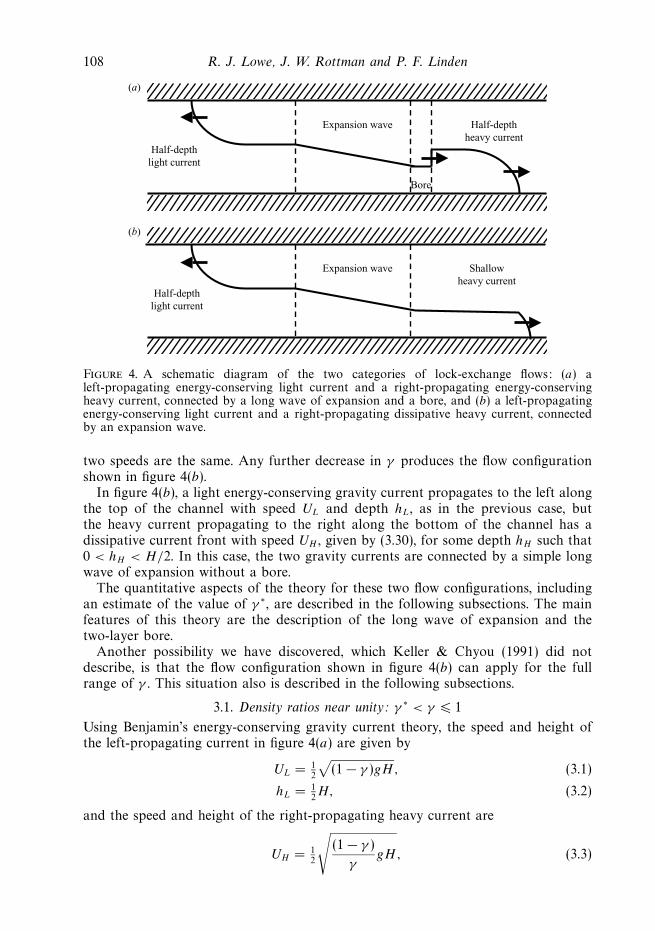
Comparisons between the theoretical shape as calculated by Benjamin (1968) andthe observed currents when γ = 0.993, 0.681 and 0.001 are shown in figure 13. Thetheoretical shape, which is strictly valid only near the front, has been extended bya straight horizontal line at mid-depth to join the two fronts. The agreement withthe observed currents appears very good for the cases with γ = 0.993 and 0.681 andnot very good for the case with γ = 0.001. Note that in this latter case, we showonly the heavy current front in the photograph; the air cavity front that is off the


(a)

(b)

(c)

Figure 13. Shadowgraph images of lock-exchange flows for three different density ratiovalues: (a) γ = 0.993, (b) γ = 0.681 and (c) γ = 0.001. The dashed lines represent thetheoretical shape of an energy-conserving gravity current. In the case with γ = 0.001, only theheavy current front is shown.

–4 –3

(a)

–2 –1 0 1 2 3 4

x/H–4 –3 –2 –1 0 1 2 3 4

(b)

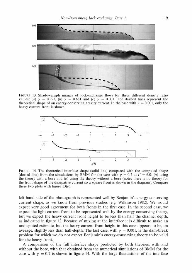
Figure 14. The theoretical interface shape (solid line) compared with the computed shape(dotted line) from the simulations by BMM for the case with γ = 0.7 at t∗ = 6.0: (a) usingthe theory with a bore and (b) using the theory without a bore (note: there is no theory forthe front shape of the dissipative current so a square front is shown in the diagram). Comparethese two plots with figure 13(b).

left-hand side of the photograph is represented well by Benjamin’s energy-conservingcurrent shape, as we know from previous studies (e.g. Wilkinson 1982). We wouldexpect very good agreement for both fronts in the first case. In the second case, weexpect the light current front to be represented well by the energy-conserving theory,but we expect the heavy current front height to be less than half the channel depth,as indicated in figure 12. Because of mixing at the interface it is difficult to make anundisputed estimate, but the heavy current front height in this case appears to be, onaverage, slightly less than half-depth. The last case, with γ = 0.001, is the dam-breakproblem for which we do not expect Benjamin’s energy-conserving theory to be validfor the heavy front.

A comparison of the full interface shape predicted by both theories, with andwithout the bore, with that obtained from the numerical simulations of BMM for thecase with γ = 0.7 is shown in figure 14. With the large fluctuations of the interface


in the simulations, which are mostly an artefact of the two-dimensionality of thesimulations, even for this value of γ , it is still difficult to determine which theory isthe more correct. Note that in figure 14(b), the theoretical dissipative heavy front, forwhich there is no theory for the front shape, is represented as a rectangle.

5. Interface stabilityAs can be observed in figures 2(a) and 3(b), in general, the light gravity-current

interface is more stable and has less mixing than does the heavy gravity-currentinterface, and this is especially true for the smaller values of γ . Similar differencesbetween the light and heavy fronts are observed in the numerical simulations ofBMM. Benjamin (1968) comments on this aspect of the lock-exchange flow andpresents a linear stability theory that explains the observations. We briefly review hisfindings here and add a few additional results from the stability theory.

Benjamin (1968) considers two layers of fluid separated by a sharp density interface.The fluid velocity in each layer is assumed to be uniform and horizontal. The densities,depths and velocities are denoted by ρi, hi and Ui , where i = 1, 2 correspond to thelower and upper layers, respectively. The undisturbed position of the interface is atz = 0 and the lower and upper boundaries are at z = −h1 and z = h2, respectively,with H = h1 + h2. The fluid is assumed to be inviscid, and the velocities are uniformso that the undisturbed flow is irrotational, except at the interface, which is a vortexsheet.

Consider a small perturbation of the interface of amplitude a of the form

η = aei(kx−ωt) = aeik(x−ct), (5.1)

travelling in the x-direction with speed c = ω/k, in which ω is the frequency and k

is the wavenumber of the wave. A relationship between c and k can be found usingpotential theory in each layer and the linearized forms of the kinematic and dynamicboundary conditions at the interface. This relationship is given by

ρ1k(c − U1)2 coth kh1 + ρ2k(c − U2)

2 coth kh2 − g(ρ1 − ρ2) = 0. (5.2)

This is a quadratic equation for c. Instability of the interface is indicated by complexconjugate roots of this equation with Im(c) > 0, taking k to be positive and real. Therequirement for this to be true is

γ tanh(kh1) + tanh(kh2) <γ

1 − γ

(U1 − U2)2

g/k. (5.3)

For an energy-conserving light current

h1 = h2 = 12H (5.4)

and

(U1 − U2)2 = (1 − γ )gH, (5.5)

and instability occurs when

tanh(kH/2) <γ

1 + γkH. (5.6)

Since 0 < γ < 1 and k is taken as positive, this inequality is satisfied for a range ofwavenumbers k > kc, where kc decreases as γ decreases, as illustrated in figure 15(a).Thus the interface is unstable to short waves, but stable to long-wave perturbations.For a cavity, when γ = 0, the interface is stable for all wavelengths.


0.2 0.4 0.6 0.8 1.0

0.2 0.4 0.6 0.8 1.0

0

2

4

6

8

10(a)

(b)

Stable

Stable

Unstable

Unstable

kH

kH

0

0.1

0.2

0.3

0.4

0.5

γ

Figure 15. The wavenumber kc as a function of the density ratio γ for which the gravitycurrent interface is neutrally stable according to linear stability theory, which separates (k, γ )space into stable and unstable regions: (a) the light gravity current and (b) the heavy gravitycurrent. Note the different vertical scales in (a) and (b).

For the heavy current in our lock-exchange flow

h2 = H − h1, (5.7)

where h1 is the depth of the current, and

(U1 − U2)2 = g

1 − γ

γh1

(2 − h1

H

)[1 −

(h1

H

)2]−1

, (5.8)

and instability occurs when

γ tanh(kh1) + tanh[k(H − h1)] <

(2 − h1

H

) [1 −

(h1

H

)2]−1

. (5.9)

Using the relationship between h1 and γ for the heavy current as determined in § 3for the lock-exchange flow without a bore, this inequality is satisfied for the range ofwavenumbers k > kc, where kc is plotted in figure 15(b). In this case, the interface isunstable to short waves, but stable for very long wave perturbations. When the lock


exchange is Boussinesq, γ = 1, or when it is a dam break, when γ = 0, the interfaceis unstable for all wavelengths.

These results imply that the interface above the heavy current is unstable to alarger range of wavelengths than the interface below the light current, especially inthe non-Boussinesq (small γ ) case. The reason for this difference is that, although the(stabilizing) density difference across the interface is the same, the higher speed of thedense current gives a greater shear across the interface. Our observations (figure 3a)are consistent with these predictions.

6. ConclusionsThe results of an experimental and theoretical study of the non-Boussinesq

lock-exchange problem have been presented. The experiments were performed ina rectangular channel using water and either a sodium iodide solution or a sodiumchloride solution as the two fluids. These combinations of fluids have density ratios(light over heavy density) in the range 0.61 to 1. A two-layer hydraulic theory isdeveloped to model the experiments. The theory assumes that a light gravity currentpropagates in one direction along the top of the channel and a heavy gravity currentpropagates in the opposite direction along the bottom of the channel. The theoryassumes that the two currents are connected by either a combination of an internalbore and an expansion wave, or just an expansion wave. The present results and theresults of two previous non-Boussinesq sets of lock-exchange experiments, both ofwhich used two different gases or a gas and a liquid as the two fluids (with densityratios in the range 0.1 to 1), and with the two-dimensional numerical simulations(with density ratios in the range 0.001 to 1) of BMM are compared with the theory.

The conclusion from a comparison of the proposed theories with our experimentalobservations and the high-resolution, two-dimensional numerical simulations of BMMis that the theory in which the two gravity currents are connected by a simple waveof expansion without an internal bore is most representative of non-Boussinesq lockexchange flows. In this case, the light current is an energy-conserving gravity currentthat occupies half the depth of the channel for all values of γ , whereas the heavycurrent is what Benjamin (1968) calls a dissipative current with a height that decreaseswith decreasing γ . This conclusion contradicts the description of the non-Boussinesqlock-exchange flow given by Keller & Chyou (1991), who concluded that the heavycurrent is energy conserving and connected to the light current by an expansion waveand an internal bore for 0.3 � γ � 1.

The theory developed here assumes that, at long times, there are two gravity currentsconnected by an expansion wave. The front conditions for the currents are analogousto hydraulic jump conditions, and they require a particular relationship between thelocal value of speed and height. These values have to adjust within these constraintsin order to match up with the expansion wave. This matching ensures that mass andmomentum are conserved. We assume that the light current is an energy-conservingBenjamin current that is locally steady. In taking this long-time approach, we haveto abandon some information about how the flow sets itself up, and therefore haveto postulate that the light current is energy conserving and steady.

It seems possible that both current fronts could be unsteady. In that case, thelong-time solution procedure would break down since all parts of the flow wouldbe unsteady. Fortunately, the experiments and numerical simulations show that ourassumptions about the light current are approximately correct. Since the expansionwave connects the two fronts, it is, therefore, necessary for the heavy current to adjust


to the flux supplied to the lower layer from the rear. This flux is set by the lightcurrent and so the energy-conserving front controls the flow on both sides of the lock.

The model proposed in this paper of an energy-conserving light current connectedto a dissipative dense current by an expansion wave is supported by calculations ofthe dissipation given in BMM. They show in their figure 13 that the fraction of thepotential energy loss that is converted to dissipation increases with time and reachesa maximum of about 12 % by the end of the simulation. In the Boussinesq case, theenergy loss in the light and dense fluids is about the same (BMM, figure 10). Muchof this dissipation is associated with the billows that form on the interface (which iswhy the fraction of the potential energy dissipated increases with time), and in thenon-Boussinesq case is significantly larger, by a factor of about 4 for γ = 0.2, for thedense current (i.e. to the right-hand side of the lock) than for the light current (seeBMM, figure 12). Thus the light front is close to energy conserving for all densityratios. Figure 16 of BMM also shows that the energy loss reduces with Re. Since ourexperiments are generally at much higher Reynolds numbers than the simulations,we expect the light front in the experiments to be close to energy conserving.

We acknowledge the productive collaboration with V. K. Birman, J. E. Martin andE. Meiburg. We thank Yi-Jiun Lin for helpful comments on an earlier draft of thispaper. This work was supported by the National Science Foundation under GrantCTS-0209194.

REFERENCES

Baines, P. G. 1995 Topographic Effects in Stratified Flows. Cambridge University Press.

Baines, W. D., Rottman, J. W. & Simpson, J. E. 1985 The motion of constant-volume air cavitiesreleased in long horizontal tubes. J. Fluid Mech. 161, 313–327.

Barr, D. I. H. 1967 Densimetric exchange flows in rectangular channels. Houille Blanche 22,619–631.

Benjamin, T. B. 1968 Gravity currents and related phenomena. J. Fluid Mech. 31, 209–248.

Birman, V., Martin, J. E. & Meiburg, E. 2005 The non-Boussinesq lock-exchange problem. Part 2.High-resolution simulations. J. Fluid Mech. 537, 125–144.

Chu, V. H. & Baddour, R. E. 1977 Surges, waves and mixing in two-layer density stratified flow.Proc. 17th Congr. Intl. Assocn Hydraul. Res. vol. 1, 303–310.

Daly, B. J. & Pracht, W. E. 1968 Numerical study of density-current surges. Phys. Fluids 11, 15–30.

Gardner, G. C. & Crow, I. G. 1970 The motion of large bubbles in horizontal channels. J. FluidMech. 43, 247–255.

Grobelbauer, H. P., Fanneløp, T. K. & Britter, R. E. 1993 The propagation of intrusion frontsof high density ratios. J. Fluid Mech. 250, 669–687.

Hartel, C., Meiburg, E. & Necker, F. 2000 Analysis and direct numerical simulation of the flow ata gravity current head. Part 1. Flow topology and front speed for slip and no-slip boundaries.J. Fluid Mech. 418, 189–212.

Huppert, H. E. & Simpson, J. E. 1980 The slumping of gravity currents. J. Fluid Mech. 99, 785–799.

Keller, J. J. & Chyou, Y.-P. 1991 On the hydraulic lock exchange problem. J. Appl. Math. Phys.42, 874–909.

Keulegan, G. H. 1958 The motion of saline fronts in still water. Natl Bur. Stand. Rep. 5813.

Klemp, J. B., Rotunno, R. & Skamarock, W. C. 1994 On the dynamics of gravity currents in achannel. J. Fluid Mech. 269, 169–198.

Klemp, J. B., Rotunno, R. & Skamarock, W. C. 1997 On the propagation of internal bores.J. Fluid Mech. 331, 81–106.

Lane-Serff, G. F., Beal, L. M. & Hadfield, T. D. 1995 Gravity current flow over obstacles.J. Fluid Mech. 292, 39–53.


Lane-Serff, G. F. & Woodward, M. D. 2001 Internal bores in two-layer exchange flows over sills.Deep-Sea Res. I 48, 63–78.

Rottman, J. W. & Linden, P. F. 2001 Gravity currents. In Stratified Flows in the Environment(ed. R. H. J. Grimshaw), pp. 87–117. Kluwer.

Rottman, J. W. & Simpson, J. E. 1983 Gravity currents produced by instantaneous releases of aheavy fluid in a rectangular channel. J. Fluid Mech. 135, 95–110.

Shin, J. O., Dalziel, S. B. & Linden, P. F. 2004 Gravity currents produced by lock exchange.J. Fluid Mech. 521, 1–34.

Simpson, J. E. & Britter, R. E. 1979 The dynamics of the head of a gravity current advancingover a horizontal surface. J. Fluid Mech. 94, 477–495.

Wilkinson, D. L. 1982 Motion of air cavities in long horizontal ducts. J. Fluid Mech. 118, 109–122.

Wood, I. R. & Simpson, J. E. 1984 Jumps in layered miscible fluids. J. Fluid Mech. 140, 329–342.

Yih, C. S. 1965 Dynamics of Nonhomogeneous Fluids. Macmillan.

Yih, C. S. & Guha, C. R. 1955 Hydraulic jump in a fluid system of two layers. Tellus 7, 358–366.

The non-Boussinesq lock-exchange problem. Part 1. Theory ...

Documents

Transcript of The non-Boussinesq lock-exchange problem. Part 1. Theory ...