978-1-4244-2824-3/08/$25.00 ©2008 IEEE 294

Proceedings of the 12th

IEEE International Multitopic Conference, Edited by Anis MK, Khan MK,

Zaidi SJH, December 23, 24, 2008, Bahria University, Karachi, Pakistan, pp 294-300, IEEE Catalog

Number: CFP08519-PRT, ISBN: 978-1-4244-2823-6, Library of Congress: 2008906985

The Multi-Stage-Lambert Scheme for Steering

a Satellite-Launch Vehicle (SLV)

Syed Arif Kamal* University of Karachi, Karachi, Pakistan; profdrakamal@gmail.com

Abstract–The determination of an orbit,

having a specified transfer time (time-of-

flight) and connecting two position vectors,

frequently referred to as the Lambert prob-

lem, is fundamental in astrodynamics. Of the

many techniques existing for solving this two-

body, two-point, time-constrained orbital

boundary-value problem, Gauss' and Lag-

range's methods were combined to obtain an

elegant algorithm based on Battin's work.

This algorithm included detection of cross-

range error. A variable TYPE, introduced in

the transfer-time equation, was flipped, to

generate the inverse-Lambert scheme. In this

paper, an innovative adaptive scheme was

pre-sented, which was called “the Multi-

Stage-Lambert Scheme”. This scheme

proposed a design of autopilot, which

achieved the pre-decided destination position

and velocity vectors for a multi-stage rocket,

when each stage was detached from the main

vehicle after it burned out, completely.

c Length of cord of the arc connecting

the points corresponding to radial

e Eccentricity of the ellipse

E Eccentric anomaly

E1 Eccentric anomaly corresponding to

the launch point

E2 Eccentric anomaly corresponding to

the final destination

f True anomaly

G Universal constant of gravitation

m Mass of spacecraft

M Mass of earth

n Unit vector, indicating normal to the

trajectory plane

p Parameter of the orbit

Flight-path angle

r Radial coördinate

r1 Radial coördinate of launch point

r2 Radial coördinate of final destination

r Radius vector in the inertial coördinate

system

Keywords–Lambert scheme, inverse-Lambert

scheme, multi-stage Lambert scheme, two-body

problem, transfer-time equation, orbital boundary-

value problem

r 2 Radius vector of final destination

t Universal time

t 1 Launch time

t 2 Time of reaching final destination

TYPE Variable expressing direction of motion

of spacecraft relative to earth’s rotation

NOMENCLATURE v Velocity vector in the inertial coördinate

System

A. Symbols (in alphabetical order) Product of universal constant of

gravitation and sum of masses of

a Semi-major axis of the ellipse spacecraft and earth

am Semi-major axis of the minimum- Time of pericenter passage

energy orbit Transfer angle —————————

*PhD; MA, Johns Hopkins, United States; Interdepart-

mental Faculty, Institute of Space and Planetary Astrophysics

(ISPA), University of Karachi; Visiting Faculty, Department

of Aeronautics and Astronautics, Institute of Space Techno-

logy, Islamabad • paper mail: Professor, Department of

Mathematics, University of Karachi, PO Box,8423, Karachi

75270, Sindh, Pakistan; telephone: +92 21 9926 1300-15 ext.

2293 • homepage: https://www.ngds-ku.org/kamal • member AIAA

Angle of inclination of velocity vector

Astrodynamical terminologies and relationships

are given in Appendices A and B, respectively.

Appendix C contains a proof of the relationship

connecting true and eccentric anomalies, providing

a justification of positive sign in front of radical.

Complete Document: https://www.ngds-ku.org/Papers/C72.pdf

THE MULTI-STAGE-LAMBERT SCHEME FOR STEERING AN SLV 295

978-1-4244-2824-3/08/$25.00 ©2008 IEEE

Proc. of 12th

IEEE INMIC, Dec. 23, 24, 2008

B. Compact Notations

In order to simplify the entries, = 21 e , =

e

e

1

1, = G (m + M), are used in the expressions

and equations.

I. INTRODUCTION

Determination of trajectory is an important

problem in astrodynamics. For a spacecraft moving

under the influence of gravitational field of earth in

free space (no air drag) the trajectory is an ellipse

with the center of earth lying at one of the foci of the

ellipse. This constitutes a standard two-body-central-

force problem, which has been treated, in detail, in

many standard text-books [1, 2]. The trick is to first

reduce the problem to two dimensions by showing

that the trajectory always lies in a plane

perpendicular to the angular-momentum vector.

Then the problem is set up in plane-polar

coördinates. Angular mo-mentum is conserved and

the problem, effectively, reduces to one-dimensional

problem involving only the variable r [3].

A problem famous in astrodynamics, called ―the

Lambert Problem‖, is based on the Lambert theorem

[4, 5]. According to this theorem the orbital-transfer

time depends only upon the semi-major axis, the

sum of the distances of the initial and the final points

of the arc from the center of force as well as length

of the line segment joining these points. Based on

this theorem a problem called the Lambert problem

is formulated. This problem deals with

determination of an orbit having a specified flight-

time and connecting the two position vectors. Battin

[6, 7] has set up the Lambert problem involving

computation of a single hypergeometric function.

Since transfer-time (time-of-flight) computation is

done on-board, it is desirable to use an algorithm

employing as few computation steps as possible.

The use of polynomials instead of actual expression

and reduction of the number of degrees of freedom

contribute towards the same goal.

An elegant Lambert algorithm, presented by

Battin, was scrutinized and omissions/oversights in

his calculations pointed out [8]. Battin’s for-

mulation, which highlighted the main principles

involved, was developed and expanded to a set of

formulae suitable for coding in the assembly

language. These formulae could be used as a

practical scheme outside the atmosphere for steering

a satellite-launch vehicle (SLV). This scheme

computes velocity and flight-path angle required at

any intermediate time to be compared with the

actual velocity and the actual flight path angle of the

spacecraft, as reported by the on-board computing

system. A spacecraft cannot reach the desired location

if cross-range error is present. Battin’s original work

does not address this issue. A mathematical

formulation was given by the author to detect cross-

range error [8]. Algorithms were developed and

tested, which indicated cross-range error. In order to

correct cross-range error velocity vector should be

perpendicular to normal to the desired trajectory plane

(i. e., the velocity must lie, entirely, in the desired

trajectory plane).

A variable TYPE was introduced in the transfer-time

equation to incorporate direction of motion of the

spacecraft [9]. This variable can take on two values,

+1 (for spacecrafts moving in the direction of rotation

of earth) and –1 (for spacecrafts moving opposite to

the direction of rotation of earth). In the inverse-

Lambert scheme, TYPE was flipped, whereas all other

parameters remained the same [8]. For an efficient

trajectory choice, a transfer time close to minimum-

energy orbital transfer time was selected. A procedure

for finding the minimum-energy orbital transfer time

is included in this work. Additionally, formulae are

given to compute the orbital parameters in which the

SLV must be locked in at a certain position, at a time,

t, based on the Lambert scheme.

In this paper, ―the Multi-Stage-Lambert Scheme‖ is

presented. In this formulation, section-wise

corrections are achieved, where destination point of

the first stage is initiating point of the second stage

and so on. In this way, position and rate satu-rations

(out of range deviations) are avoided. A similar

formulation was, earlier, given for the Q System [9].

II. STATEMENT OF THE PROBLEM

In order to choose a particular trajectory on which

the spacecraft could be locked so as to reach a certain

point one must select a certain parameter to fix this

trajectory out of the many possible ones connecting

the two points. One is, therefore, interested to put the

Kepler equation in such a form so as to make it

computationally efficient utilizing hypergeometric

functions or quadratic functions instead of circular

functions (sine or co-sine, etc.). This equation should

express transfer time between these two points in

terms of a series or a polynomial, and another formula

should be available to compute flight-path angle,

correspon-ding to this transfer time. Velocity

desirable for a particular trajectory may, then, be

computed on- board using this formula and compared

with velocity of the spacecraft obtained from

integration of acceleration information, which is

available from on-board accelerometers and rate

velocity board

296 KAMAL

978-1-4244-2824-3/08/$25.00 ©2008 IEEE

Proc. of 12th

IEEE INMIC, Dec. 23, 24, 2008

gyroscopes.

III. THE LAMBERT THEOREM

In 1761 Johann Heinrich Lambert, using a geo-

metrical argument, demonstrated that the time taken

to traverse any arc (now called transfer time),

12 tt , is a function, only, of the major axis, a, the

arc, )( 21 rr , and length of chord of the arc, c , for

elliptical orbits, i. e.,

12 tt = ),,( 21 acrrf

The symbol, f, is used to express functional

relationship in the above equation (do not confuse

with true anomaly). Therefore, one notes that the

transfer time does not depend on true or eccentric

anomalies of the launch point or the final desti-

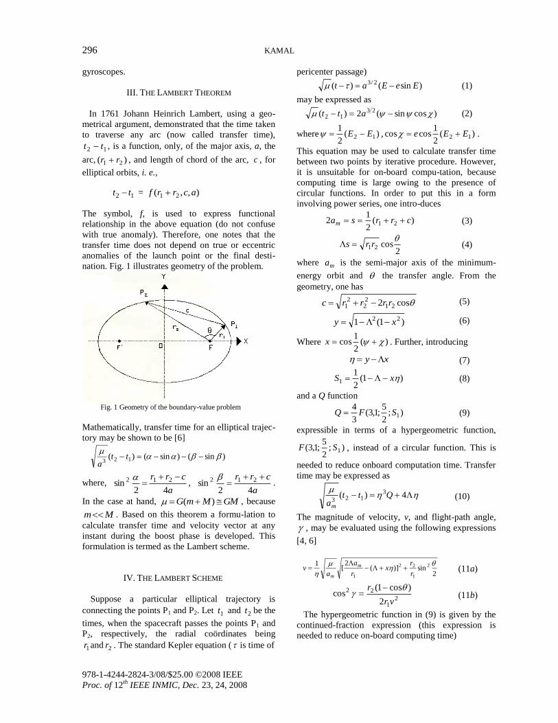
nation. Fig. 1 illustrates geometry of the problem.

Fig. 1 Geometry of the boundary-value problem

Mathematically, transfer time for an elliptical trajec-

tory may be shown to be [6]

)sin()sin()( 123

tt

a

where, a

crr

42sin 212

, a

crr

42sin 212

.

In the case at hand, GMMmG )( , because

Mm . Based on this theorem a formu-lation to

calculate transfer time and velocity vector at any

instant during the boost phase is developed. This

formulation is termed as the Lambert scheme.

IV. THE LAMBERT SCHEME

Suppose a particular elliptical trajectory is

connecting the points P1 and P2. Let 1t and 2t be the

times, when the spacecraft passes the points P1 and

P2, respectively, the radial coördinates being

1r and 2r . The standard Kepler equation ( is time of

pericenter passage)

)sin()( 2/3 EeEat (1)

may be expressed as

)cossin(2)( 2312 att (2)

where )(2

112 EE , )(

2

1coscos 12 EEe .

This equation may be used to calculate transfer time

between two points by iterative procedure. However,

it is unsuitable for on-board compu-tation, because

computing time is large owing to the presence of

circular functions. In order to put this in a form

involving power series, one intro-duces

)(2

12 21 crrsam (3)

2cos21

rrs (4)

where ma is the semi-major axis of the minimum-

energy orbit and the transfer angle. From the

geometry, one has

cos2 2122

21 rrrrc (5)

)1(1 22 xy (6)

Where )(2

1cos x . Further, introducing

xy (7)

)1(2

11 xS (8)

and a Q function

);2

5;1,3(

3

41SFQ (9)

expressible in terms of a hypergeometric function,

);2

5;1,3( 1SF , instead of a circular function. This is

needed to reduce onboard computation time. Transfer

time may be expressed as

4)( 3123

Qttam

(10)

The magnitude of velocity, v, and flight-path angle,

, may be evaluated using the following expressions

[4, 6]

2sin)](

2[

1 2

1

22

1

r

rx

r

a

av m

m

(11a)

21

22

2

)cos1(cos

vr

r

(11b)

The hypergeometric function in (9) is given by the

continued-fraction expression (this expression is

needed to reduce on-board computing time)

THE MULTI-STAGE-LAMBERT SCHEME FOR STEERING AN SLV 297

978-1-4244-2824-3/08/$25.00 ©2008 IEEE

Proc. of 12th

IEEE INMIC, Dec. 23, 24, 2008

....17

10815

1813

7011

49

407

65

183

3);

2

5;1,3(

1

1

1

1

1

1

11

S

S

S

S

S

S

SSF

About 100 terms are needed to get an accuracy of

10-4

.

To compute the transfer time corresponding to the

minimum energy orbit connecting the current posi-

tion and the final destination one uses the transfer-

time equation (11), with 0x substituted in (8),

corresponding to maa and solves it using

Newton-Raphson method. Transfer time in the

Lambert algorithm must be set close to this time.

Fig. 2 shows the flow chart of Lambert algorithm.

Fig. 2 Flow chart of the Lambert scheme

V. CROSS-RANGE-ERROR DETECTION

(MATHEMATICAL MODEL)

For no cross-range error, velocity of the space-

craft must lie in the plane containing 2rr (the tra-

jectory plane). In other words, the velocity vector

must make an angle of 900 with normal to the

trajectory plane. This is equivalent to [8]

0).( 2 rrv (12)

which says that v (current velocity), r (current

position) and 2r (position of destination) are co-

planar. For no cross-range error, the angle of

inclination, , between the velocity vector, v , and

normal to the trajectory, n , must be 900. In the

Lambert scheme a subroutine computes devi-ation of

from 900. Extended-cross-product steering [10],

dot-product steering [11] and ellipse-orientation

steering [12] could be used to eliminate cross-range

error.

VI. THE INVERSE-LAMBERT SCHEME

Transfer-time equation between two points having

eccentric anomalies 1E and 2E , (corresponding to

times 1t and 2t , respectively) may be expressed as [8]

12 tt

])][sin()sin[( 1122

3

TYPEEeEEeEa

(13)

The variable TYPE has to be introduced because

the Kepler equation is derived on the assumption that t

increases with the increase in f. Therefore, the

difference

)]sin()sin[( 1122 EeEEeE

shall come out to be negative for spacecrafts orbiting

in a sense opposite to rotation of earth. The variable TYPE ensures that the transfer time (which is the

physical time) remains positive in all situations by

adapting the convention that TYPE =+1 for

spacecrafts moving in the direc-tion of earth’s

rotation, whereas, TYPE = –1 for spacecrafts moving

opposite to the direction of earth’s rotation. This

becomes important in computing correct flight-path

angles in the Lambert scheme.

If one wants to put another spacecraft in the same

orbit as the original spacecraft, but moving in the

opposite direction, one can use the inverse- Lambert

scheme. This can be accomplished by flipping sign of

the variable, TYPE , whereas all the other parameters

remain the same. Burns and Sherock [13]

try to

accomplish the same objective by a three-degree-of-

freedom interceptor simulation designed to rendez-

vous with a ballistic target: position and velocity

matching, no flipping of TYPE. The strategy put for-

298 KAMAL

978-1-4244-2824-3/08/$25.00 ©2008 IEEE

Proc. of 12th

IEEE INMIC, Dec. 23, 24, 2008

ward by this author was simpler [8]: orbit matching,

flipping of TYPE. The inverse-Q system has, also,

been proposed by the author to accomplish the same

objective [9]. Do not confuse Q system with the

symbol Q introduced in (9).

VII. THE MULTI-STAGE-LAMBERT SCHEME

Let us consider a three-stage rocket. Destination

point of the first (second) stage is the initiating point

of the second (third) stage. Mathematically,

initialfinalinitialfinal vvvv ,3,2,2,1 ; (14a)

initialfinalinitialfinal ,3,2,21 ; (14b)

Equations (11a, b) can be used to compute velocities

and flight-path angles at the initiating and

destination points of various stages. By using these

section-wise corrections, one can avoid position

saturation and rate saturation.

VIII. DISCUSSION AND CONCLUSIONS

The Lambert problem is a fixed-transfer-time-

boundary-value problem. The Lambert-scheme

formulations available in literature run into prob-

lems in terms of computing correct flight-path

angles and velocities, in particular, for spacecrafts

moving opposite to earth rotation because of defini-

tion of time in the Kepler equation. This problem

was resolved by introducing a variable, TYPE, in the

transfer-time equation. This, also, led to a natural

formulation of the inverse-Lambert scheme. The

Lambert scheme is applicable in free space, in the

absence of atmospheric drags, for burnout times

large as compared to on-board computation time

(for example, if the burnout time for a given flight is

18 second and the computation time is 1 second,

there may not be enough time to utilize this

scheme). This is needed to allow sufficient time for

the control decisions to be taken and implemented

before the rocket runs out of fuel. Detection of

cross-range error is incorporated in this formulation.

It is assumed that rocket is fired in the vertical

position so as to get out of the atmosphere with

minimum expenditure of fuel. Later, in free space

this scheme is applied to correct the path of rocket.

Since the rocket remains in free space for most of

the time, this method may be useful in calculating

the desired trajectory.

The Lambert scheme is an explicit scheme, which

generates a suitable trajectory under the influence of

an inverse-square-central-force law (gravitational

field of earth) provided one knows the latitudes and

the longitudes of launch point and of destination as

well as the transfer time (time spent by the spacecraft

to reach destination).

The Lambert scheme is an explicit scheme, which

generates a suitable trajectory under the influence of

an inverse-square-central-force law (gravitational field

of earth) provided one knows the latitudes and the

longitudes of launch point and of destination as well

as the transfer time.

ACKNOWLEDGMENT

This work was made possible, in part, by Dean's

Research Grant awarded by University of Karachi,

which is, gratefully, acknowledged.

APPENDIX A: ASTRODYNAMICAL TERMINOLOGIES

Down-range error is the error in the range assuming

that the vehicle is in the correct plane; cross-range

error is the offset of the trajectory from the desired

plane. An unwanted pitch movement shall produce

down-range error; an unwanted yaw movement shall

produce cross-range error.

For an elliptical orbit true anomaly, f, is the polar

angle measured from the major axis ( PFX in Fig.

3). Through the point P (current pos

Fig. 3 Justification of the positive sign in

position of spacecraft, rPFm , the radial coör-

dinate) erect a perpendicular on the major axis. Q is

the intersection of this perpendicular with a circums-

cribed auxiliary circle about the orbital path. The

angle, QOF (cf. Fig.3) is called the eccentric

anomaly, E.

THE MULTI-STAGE-LAMBERT SCHEME FOR STEERING AN SLV 299

978-1-4244-2824-3/08/$25.00 ©2008 IEEE

Proc. of 12th

IEEE INMIC, Dec. 23, 24, 2008

For this orbit, pericenter, the point on the major

axis, which is closest to the force center (point A in

Fig. 3), is chosen as the point at which f = 0.

Apocenter is the opposite point on the major axis,

which is farthest from the force center (point A in

Fig. 3). The line joining the pericenter and the

apocenter is called the line of apsides.

APPENDIX B: ASTRODYNAMICAL RELATIONHIPS

Some useful relationships among radial

coördinate, eccentric anomaly, eccentricity and

semi-major axis for an elliptical orbit are listed

below:

)cos1( Eear (B1a)

)(coscos eEafr (B1b)

Eafr sinsin (B1c)

2cos)1(

2cos

Eea

fr (B1d)

2sin)1(

2sin

Eea

fr (B1e)

The following may be useful in converting circular

functions involving true anomalies to those

involving eccentric anomalies and vice versa.

Ee

eEf

cos1

coscos

(B2a)

fe

efE

cos1

coscos

(B2b)

Ee

Ef

cos1

sinsin

(B2c)

fe

fE

cos1

sinsin

(B2d)

2tan

2tan

Ef (B2e)

In Appendix C, the last relation is proved and a

justi-fication is given for the positive sign taken in

front of the square root appearing in the expression

for .

APPENDIX C: RELATION CONNECTING ECCENTRIC

ANOMALY TO TRUE ANOMALY

In Fig. 3, semi-minor axis of the ellipse, b, is related

to a by ab . Do not confuse the point Q in Fig. 3

with the quantity Q defined in (9). Using the

relations fe

pr

cos1 and )1( 2eap , one may

write, )1()cos1( 2eafer . Rearranging

reafer )1(cos 2

Adding er to both sides and using (B1a) on the right-

hand side, one gets

)cos1)(1()cos1( Eeafr (C1)

Subtracting er from both sides and using (B1a) on the

right-hand side, one gets

)cos1)(1()cos1( Eeafr (C2)

Dividing (C2) by (C1)

)cos1)(1(

)cos1)(1(

cos1

cos1

Ee

Ee

f

f

Using the identities

2sin2cos1 2 f

f

2cos2cos1 2 f

f

with similar results for the expressions )cos1( E and

)cos1( E , one sees that the above equation reduces

to

2tan

1

1

2tan 22 E

e

ef

which implies

2tan

1

1

2tan

E

e

ef

Below, it is justified that only positive sign with the

radical gives the correct answer. Consider ORF (cf.

Fig. 3). One notes that,

E 222

E

Further, 0E 0f ; 0E 0f .

Therefore, 2

fand

2

E have the same sign. When

022

E, 0

2tan

E, 0

2tan

f, which implies

that positive sign with the radical should be chosen.

Similarly,

22

0

E

, 02

tan E

, 02

tan f

and, hence, positive sign with the radical is the correct

choice.

Two-body problem can be handled elegantly by

using the elliptic-astrodynamical-coördinate mesh [14,

15]. One discovers additional constants of motion if

the problem is set up using this formulation [16].

300 KAMAL

978-1-4244-2824-3/08/$25.00 ©2008 IEEE

Proc. of 12th

IEEE INMIC, Dec. 23, 24, 2008

REFERENCES formulation of extended-cross-product steer-

ing,‖ Proceedings of the First International

[1] H. Goldstein, Classical Mechanics, 2nd

Bhurban Conference on Applied Sciences and

ed., Reading, MA: Addison Wesley, Technologies (IBCAST 2002), vol. 1, Advanced

1981, pp. 70-102 Materials, Computational Fluid Dynamics and

[2] J. B. Marion, Classical Dynamics of Control Engineering, ed. H. R. Hoorani, A.

Particles and Systems, 2nd

ed., New Munir, R. Samar and S. Zahir, National Center for

York: Academic, 1970, pp. 243-278 Physics, Bhurban, 2003, pp. 167-177£

[3] J. T. Wu, ―Orbit determination by sol- [11] S. A. Kamal, ―Dot-product steering: a new con-

ving for gravity parameters with multi- trol law for satellites and spacecrafts,‖ Proceed-

ple arc data,‖ Journal of Guidance, ings of the First International Bhurban Confer-

Control and Dynamics, vol. 15, pp. 304 ence on Applied Sciences and Technologies

-313, February 1992 (IBCAST 2002), vol. 1, Advanced Materials,

[4] R. H. Battin, An Introduction to the Computational Fluid Dynamics and Control Eng-

Mathematics and (the) Methods of Astro- ineering, ed. H. R. Hoorani, A. Munir, R. Samar

dynamics, 1st ed., Washington, DC: and S. Zahir, National Center for Physics, Bhur-

AIAA, 1987, pp. 276-342α ban, 2003, pp. 178-184

¥

[5] R. Deusch, Orbital Dynamics of Space [12] S. A. Kamal, “Ellipse-orientation steering: a

Vehicles, Englewood Cliffs, NJ: Pren- control law for spacecrafts and satellite-launch

tice Hall, 1963, pp. 20-22 vehicles (SLV),‖ Space Science and Challenges

[6] R. H. Battin, ―Lambert’s problem re- of the Twenty-First Century, ISPA-SUPARCO

visited,‖ AIAA Journal, vol. 15, pp. 707 Collaborative Seminar (in connection with

-713, May 1977 World Space Week), University of Karachi,

[7] R. H. Battin and R. M. Vaughan, ―An 2005 (invited lecture)€

elegant Lambert algorithm,‖ Journal of [13] S. P. Burns and J. J. Scherock, ―Lambert-gui-

Guidance and Control, vol. 7, pp. 662- dance routine designed to match position and

670, June 1984 velocity of ballistic target,‖ Journal of Gui-

[8] S. A. Kamal, ―Incorporating cross-range dance, Control and Dynamics, vol. 27, pp. 989-

error in the Lambert scheme,‖ the Tenth 996, June 2004

National Aeronautical Conference, Coll- [14] S. A. Kamal, ―Planetary-orbit modeling based on

ege of Aeronautical Engineering, PAF astrodynamical coördinates,‖ the Pakistan Insti-

Academy, Risalpur, 2006, pp. 255-263µ tute of Physics International Conference, Lahore,

[9] S. A. Kamal and A. Mirza, “The multi- 1997, pp. 28-29

stage-Q system and the inverse-Q sys- [15] S. A. Kamal, ―Use of astrodynamical coördinates

tem for possible application in satellite- to study bounded-keplarian motion,‖ the Fifth Int-

launch vehicle (SLV),‖ Proceedings of ernational Pure Mathematics Conference, the

the Fourth International Bhurban Con- Quaid-é-Azam University and the Pakistan Math-

ference on Applied Sciences and Tech- ematical Society, Islamabad, 2004

Technologies (IBCAST 2005), vol. 3, [16] S. A. Kamal, ―Strong Noether’s theorem: applica-

Control and Simulation, ed. S. I. Hussain, ions in astrodynamics,‖ the Second Symposium on

A. Munir, J. Kayani, R. Samar and M. A. Cosmology, Astrophysics and Relativity, Center

Khan, National Center for Physics, Bhur- for Advanced Mathematics and Physics, NUST

ban, 2006, pp. 27-33 and National Center for Physics, Rawalpindi,

[10] S. A. Kamal, ―Incompleteness of cross- 2004, p. 2

Product steering and a mathematical αReview: https://www.ngds-ku.org/Papers/Battin.pdf

€Abstract: https://www.ngds-ku.org/Presentation/Ellipse.pdf

µFull text: https://www.ngds-ku.org/Papers/C67.pdf

Abstract: https://www.ngds-ku.org/Presentation/Planetrary.pdf

Full text: https://www.ngds-ku.org/Papers/C66.pdf

Abstract:

£Full text: https://www.ngds-ku.org/Papers/C56.pdf https://www.ngds-ku.org/Presentations/Astrodynamical.pdf

¥Full text: https://www.ngds-ku.org/Papers/C55.pdf

Abstract: https://www.ngds-ku.org/Presentation/Noether.pdf

Web address of this document (author’s homepage): https://www.ngds-ku.org/Papers/C72.pdf