The New Keynesian Hybrid Phillips Curve: An … of Canada Working Paper 2004-31 August 2004 The New...
36
Bank of Canada Banque du Canada Working Paper 2004-31 / Document de travail 2004-31 The New Keynesian Hybrid Phillips Curve: An Assessment of Competing Specifications for the United States by David Dupuis
Transcript of The New Keynesian Hybrid Phillips Curve: An … of Canada Working Paper 2004-31 August 2004 The New...

Bank of Canada Banque du Canada
Working Paper 2004-31 / Document de travail 2004-31
The New Keynesian Hybrid Phillips Curve:An Assessment of Competing Specifications
for the United States
by
David Dupuis

ISSN 1192-5434
Printed in Canada on recycled paper

Bank of Canada Working Paper 2004-31
August 2004
The New Keynesian Hybrid Phillips Curve:An Assessment of Competing Specifications
for the United States
by
David Dupuis
International DepartmentQuebec Regional Office
Bank of Canada1501 McGill College
Montréal, QC H3A [email protected]
The views expressed in this paper are those of the author.No responsibility for them should be attributed to the Bank of Canada.


iii
Contents
Acknowledgements. . . . . . . . . . . . . . . . . . . . . . . . . . . . . . . . . . . . . . . . . . . . . . . . . . . . . . . . . . . . ivAbstract/Résumé. . . . . . . . . . . . . . . . . . . . . . . . . . . . . . . . . . . . . . . . . . . . . . . . . . . . . . . . . . . . . . . v
1. Introduction . . . . . . . . . . . . . . . . . . . . . . . . . . . . . . . . . . . . . . . . . . . . . . . . . . . . . . . . . . . . . . 1
2. The New Keynesian Phillips Curve: Basic Derivation . . . . . . . . . . . . . . . . . . . . . . . . . . . . . 1
3. The New Hybrid Phillips Curve . . . . . . . . . . . . . . . . . . . . . . . . . . . . . . . . . . . . . . . . . . . . . . 4
3.1 The model . . . . . . . . . . . . . . . . . . . . . . . . . . . . . . . . . . . . . . . . . . . . . . . . . . . . . . . . . . . 4
3.2 Estimation of the new hybrid Phillips curve. . . . . . . . . . . . . . . . . . . . . . . . . . . . . . . . . 6
3.3 Robustness analysis . . . . . . . . . . . . . . . . . . . . . . . . . . . . . . . . . . . . . . . . . . . . . . . . . . . 8
4. The Polynomial Adjustment-Cost Approach. . . . . . . . . . . . . . . . . . . . . . . . . . . . . . . . . . . . 11
4.1 The model . . . . . . . . . . . . . . . . . . . . . . . . . . . . . . . . . . . . . . . . . . . . . . . . . . . . . . . . . .11
4.2 Estimates of the PAC model . . . . . . . . . . . . . . . . . . . . . . . . . . . . . . . . . . . . . . . . . . . . 12
5. Forecasting Inflation: A Look at Competing Approaches for the United States. . . . . . . . . 17
6. Conclusion . . . . . . . . . . . . . . . . . . . . . . . . . . . . . . . . . . . . . . . . . . . . . . . . . . . . . . . . . . . . . . 18
References. . . . . . . . . . . . . . . . . . . . . . . . . . . . . . . . . . . . . . . . . . . . . . . . . . . . . . . . . . . . . . . . . . . 20
Figures. . . . . . . . . . . . . . . . . . . . . . . . . . . . . . . . . . . . . . . . . . . . . . . . . . . . . . . . . . . . . . . . . . . . . . 22
Appendix . . . . . . . . . . . . . . . . . . . . . . . . . . . . . . . . . . . . . . . . . . . . . . . . . . . . . . . . . . . . . . . . . . . 27

iv
Acknowledgements
Thanks to Hafedh Bouakez, Thérèse Laflèche, Robert Lafrance, René Lalonde, Graydon Paulin,
Jean-François Perrault, James Powell, Larry Schembri, and participants at an International
Department seminar and at the 2004 CEA conference in Toronto for their helpful comments and
suggestions.
v
e
and
002),
ally
icing
n that
ian
a, b),
hybrid
n the
ueur
lí,
nent
exte de
plan
t de
de
t b),
uvelle
Abstract
Inflation forecasting is fundamental to monetary policy. In practice, however, economists ar
faced with competing goals: accuracy and theoretical consistency. Recent work by Fuhrer
Moore (1995), Galí and Gertler (1999), Galí, Gertler, and Lopez-Salido (2001), Sbordone (2
and Kozicki and Tinsley (2002a, b) suggests that the two objectives need not be mutually
exclusive in the context of inflation forecasts. The New Keynesian Phillips curve is theoretic
appealing, because its purely forward-looking specification is based on a model of optimal pr
behaviour with rational expectations. This specification, however, does not properly capture
observed inflation persistence. The author estimates three structural models of U.S. inflatio
incorporate price frictions to justify the presence of lags in the forward-looking New Keynes
Phillips curve. The models, based on Galí and Gertler (1999) and Kozicki and Tinsley (2002
are tested on the basis of forecast performances. The results show that the new Keynesian
Phillips curve with the output gap as an explanatory variable performs marginally better tha
two alternative specifications.
JEL classification: E31Bank classification: Inflation and prices; Economic models
Résumé
La prévision de l’inflation est fondamentale pour la politique monétaire. Dans la pratique,
toutefois, les économistes doivent s’efforcer de concilier deux objectifs : l’exactitude et la rig
théorique. Des travaux récents de Fuhrer et Moore (1995), de Galí et Gertler (1999), de Ga
Gertler et Lopez-Salido (2001), de Sbordone (2002) et de Kozicki et Tinsley (2002a et b) don
à penser que les deux objectifs ne sont pas forcément mutuellement exclusifs dans le cont
la prévision de l’inflation. La nouvelle courbe de Phillips keynésienne est séduisante sur le
théorique, car sa formulation strictement prospective repose sur un modèle de tarification
optimale où les anticipations sont rationnelles. Cette spécification ne permet pas cependan
saisir la persistance de l’inflation. L’auteur estime trois modèles structurels de l’inflation aux
États-Unis qui intègrent des frictions relatives aux prix afin de tenir compte de la présence
retards dans la formulation prospective de la nouvelle courbe de Phillips keynésienne. Les
modèles, qui s’inspirent de ceux de Galí et Gertler (1999) et de Kozicki et Tinsley (2002a e
sont évalués sur la base de la qualité de leurs prévisions. Les résultats montrent que la no
courbe de Phillips hybride keynésienne où l’écart de production intervient à titre de variable
explicative permet de prévoir l’inflation un peu mieux que les deux autres formulations
envisagées.
Classification JEL : E31Classification de la Banque : Inflation et prix; Modèles économiques


1
gests
he
vel of
and
price
e the
(1999)
ee
ry
ree
nts and
f each
1. Introduction
In forecasting, economists are often faced with competing goals: accuracy and theoretical
consistency. This is of particular importance in the case of inflation, which is fundamental to
monetary policy. Recent work by Fuhrer and Moore (1995), Galí and Gertler (1999), Galí,
Gertler, and Lopez-Salido (2001), Sbordone (2002), and Kozicki and Tinsley (2002a, b) sug
that the two objectives need not be mutually exclusive in the context of inflation forecasts. T
New Keynesian Phillips curve is theoretically appealing, because its purely forward-looking
specification is based on a model of optimal pricing behaviour with rational expectations.
The literature, however, has found that, under such a specification, inflation displays a low le
persistence, which is inconsistent with observed inflation dynamics.1 Alternative and more
general specifications of pricing frictions lead to Phillips curves that contain additional lags
expected leads of inflation. By assuming the presence of adjustment costs associated with
changes, these specifications are more consistent with observed inflation and do not violat
assumption of rational expectations. Such specifications are proposed by Galí and Gertler
and Kozicki and Tinsley (2002a, b).
The goal of this paper is to identify, among three competing model specifications, which
formulation of the hybrid Phillips curve provides the best forecasts of U.S. inflation. The thr
competing specifications are: a marginal cost-based hybrid Phillips curve (HPCmc) proposed by
Galí and Gertler (1999), its output-gap counterpart (HPCgap), and a polynomial adjustment-cost
(PAC) specification proposed by Kozicki and Tinsley (2002a, b). Section 2 reviews the theo
behind the New Keynesian Phillips curve and frictions on price adjustments central to all th
approaches. Section 3 presents and estimates both hybrid Phillips curves. Section 4 prese
estimates the PAC specification. Section 5 tests and compares the forecasting properties o
model with other competing specifications. Section 6 offers some conclusions.
2. The New Keynesian Phillips Curve: Basic Derivation
In the basic model, the business sector is assumed to be composed of a continuum of
monopolistically competitive firms, indexed byi, each producing a differentiated good,Yi,t at time
t, with the production function given byYi,t = ZtLi,t, whereZt corresponds to total factor
productivity.2 In this context, households are being paid the nominal wage,Wt, and each firm
1. See, for example, Galí and Gertler (1999).2. For simplicity, this model does not include capital.
2
uld
here
,
d
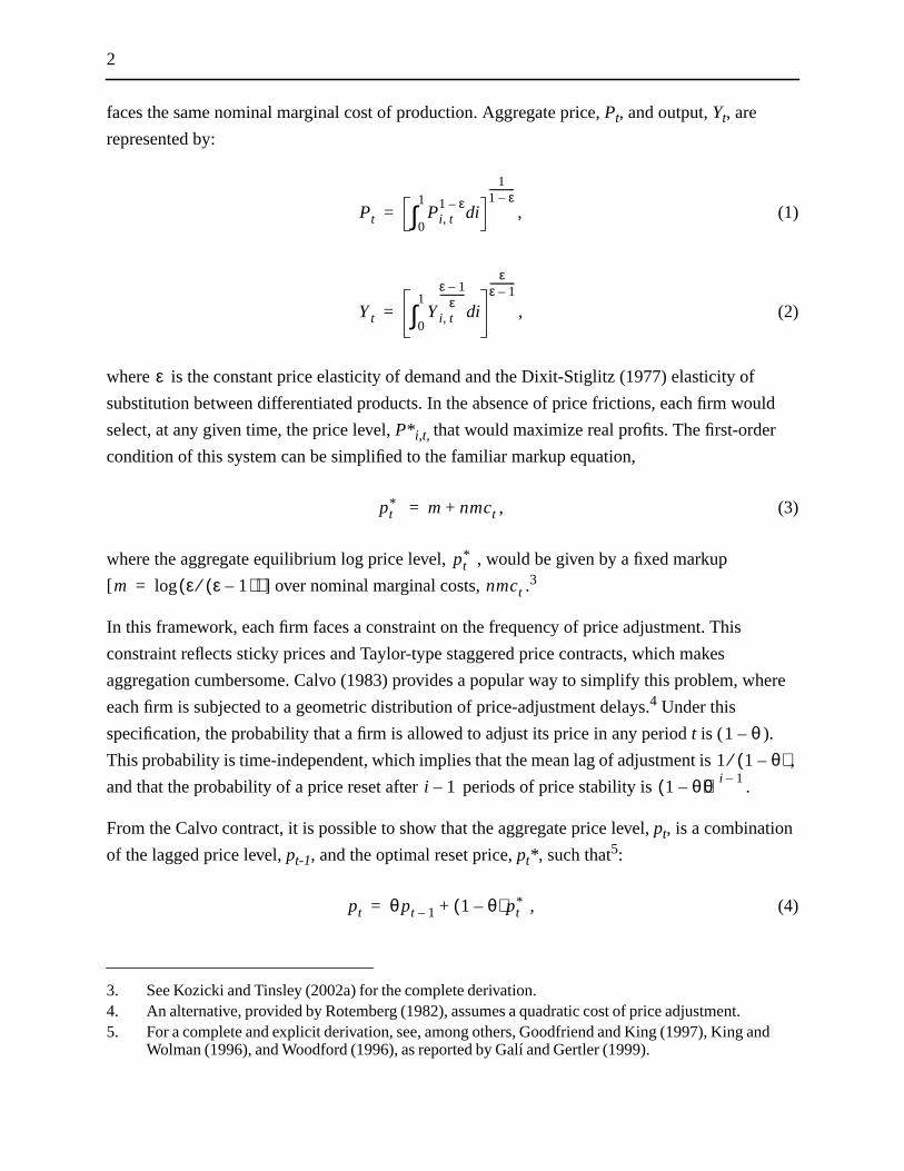
faces the same nominal marginal cost of production. Aggregate price,Pt, and output,Yt, are
represented by:
, (1)
, (2)
where is the constant price elasticity of demand and the Dixit-Stiglitz (1977) elasticity of
substitution between differentiated products. In the absence of price frictions, each firm wo
select, at any given time, the price level,P*i,t, that would maximize real profits. The first-order
condition of this system can be simplified to the familiar markup equation,
, (3)
where the aggregate equilibrium log price level, , would be given by a fixed markup
[ ] over nominal marginal costs, .3
In this framework, each firm faces a constraint on the frequency of price adjustment. This
constraint reflects sticky prices and Taylor-type staggered price contracts, which makes
aggregation cumbersome. Calvo (1983) provides a popular way to simplify this problem, w
each firm is subjected to a geometric distribution of price-adjustment delays.4 Under this
specification, the probability that a firm is allowed to adjust its price in any periodt is ( ).
This probability is time-independent, which implies that the mean lag of adjustment is
and that the probability of a price reset after periods of price stability is .
From the Calvo contract, it is possible to show that the aggregate price level,pt, is a combination
of the lagged price level,pt-1, and the optimal reset price,pt* , such that5:
, (4)
3. See Kozicki and Tinsley (2002a) for the complete derivation.4. An alternative, provided by Rotemberg (1982), assumes a quadratic cost of price adjustment.5. For a complete and explicit derivation, see, among others, Goodfriend and King (1997), King an
Wolman (1996), and Woodford (1996), as reported by Galí and Gertler (1999).
Pt Pi t,1 ε–
id0
1
∫1
1 ε–-----------
=
Yt Yi t,
ε 1–ε
-----------
id0
1
∫
εε 1–-----------
=
ε
pt* m nmct+=
pt*
m ε ε 1–( )⁄( )log= nmct
1 θ–
1 1 θ–( )⁄i 1– 1 θ–( )θi 1–
pt θ pt 1– 1 θ–( ) pt*+=

3
a firm
h
se of
emain
inal
will
ost in
ce of
I
urve
where the variables are expressed in deviation from the steady-state inflation rate. Then, for
that resets its price at timet to maximize expected discounted profits, the optimal reset price,
given the Calvo contract, can be expressed as6:
, (5)
where is a discount factor.
It follows that firms allowed to reset prices at timet will take account of the expected future pat
of nominal marginal cost (expressed in per cent deviation from steady state), in view of the
possibility that the new reset price might be subject to future adjustment constraints. In the ca
perfect price flexibility ( ), firms merely adjust prices proportionately to movements in
current marginal costs. As the degree of price rigidity, , increases, prices are expected to r
fixed for an extended period of time, and the firm will place more weight on expected marg
costs in setting current prices.
Hence, a firm’s real marginal cost, given cost minimization and Cobb-Douglas technology,
equal the real wage divided by the marginal product of labour. Therefore, the real marginal c
t + k for a firm that has optimally set prices int is given by,
, (6)
where and represent output and employment for a firm that has set prices int at
the optimal value, . Individual firm marginal cost, however, is not observable in the absen
firm level data. It is therefore helpful to define the observable average marginal cost as:
. (7)
Following Woodford (1996), Galí, Gertler, and Lopez-Salido (2001), and Sbordone (2002),
assume that the Cobb-Douglas production technology framework and isoelastic demand c
obtains the following log-linear relationship between and :
6. Since all variables are expressed in deviation from steady state, the constant markup (m) drops out ofequation (5).
pt* 1 βθ–( ) βθ( )k
Et nmct k+{ }k 0=
∞
∑=
β
θ 0=
θ
MCt t k+,Wt k+ Pt k+⁄( )
1 α–( ) Yt t, k+ Nt t k+,⁄( )-----------------------------------------------------------=
Yt t, k+ Nt t k+,Pt
*
MCt
Wt Pt⁄( )1 α–( ) Yt Nt⁄( )
--------------------------------------≡
MCt t k+, MCt

4
),
illips
ature
nce,
ade
tract
ill
eir
ce
e-
, (8)
where and are the log deviations of and from their respective
steady-state values. It follows that, in the limiting case, where technology is linear (i.e.,
all firms will face the same marginal cost.
Combining equations (4), (5), and (8), the Calvo formulation leads to the New Keynesian Ph
curve, which relates to the real marginal cost and takes the following form:
, (9)
where the coefficient
(10)
is a function of the frequency of price adjustment, , a discount factor, , the degree of curv
of the production function, , and the elasticity of demand, .
3. The New Hybrid Phillips Curve
3.1 The model
Galí and Gertler (1999) have established that, in the New Keynesian Phillips curve, inflation
displays a low level of persistence that is inconsistent with observed inflation dynamics. He
following Galí and Gertler (1999) and Galí, Gertler, and Lopez-Salido (2001), a departure is m
from the basic Calvo model to allow for sticky-price adjustment. Specifically, the Calvo con
is modified to allow two types of firms to coexist in the model. A subsample of firms, , w
have forward-looking price-setting behaviour “à la Calvo,” while the remaining firms will set th
prices using a backward-looking rule of thumb based on the recent history of aggregate pri
inflation. The aggregate price level is then given by:
, (11)
where is an index of prices set in periodt, based on the forward- and backward-looking pric
setters’ behaviour such that,
mcˆt t k+, mcˆ
t k+εα
1 α–------------ pt
* pt k+–( )–=
mcˆt t k+, mcˆ
t k+ MCt t k+, MCt
α 0=
πt κEt πt 1+{ } λmcˆt+=
λ 1 θ–( ) 1 βθ–( ) 1 α–( )θ 1 α ε 1–( )+[ ]
-------------------------------------------------------≡
θ βα ε
1 ω–
pt θ pt 1– 1 θ–( ) pt*+=
pt*

5
ard-
d
n (5),
firms
s
ause
ed on
etters
cent
he
) the
um,lags
, (12)
where is the price set by the backward-looking rule of thumb, is the price set by forw
looking firms, and is the degree of “backward-lookingness.” For the purpose of the hybri
Phillips curve specification, forward-looking firms behave exactly as in the basic Calvo
framework described earlier. Consequently, their behaviour can be expressed as in equatio
such that,
. (13)
For backward-looking firms, we adopt Galí and Gertler’s assumptions and posit that these
follow a rule of thumb based on recent aggregate pricing behaviour, which can be stated a
follows7:
. (14)
Intuitively, since forward-looking firms set prices as a markup over marginal costs, and bec
they must lock in prices for (perhaps) more than one period, a firm’s pricing decision is bas
the expected future behaviour of marginal costs. Correspondingly, backward-looking price-s
will fix their prices according to the equilibrium price in the previous period, corrected for re
inflation.8
Combining equations (9) and (11) through (14), the reduced-form empirical formulation of t
hybrid Phillips curve is given by:
, (15)
where ,
,
,
with .
7. Galí and Gertler assume (i) no persistent deviations between the rule and optimal behaviour; (iiprice in periodt given by the rule depends only on information datedt-1 or earlier; and (iii) firms areunable to discern whether any individual competitor is backward or forward looking.
8. This process is akin to the indexation of a backward-looking rule of thumb. Christiano, Eichenbaand Evans (1997) use this specification to justify, on the basis of theory, the presence of inflationin the New Keynesian Phillips curve.
pt* ωpt
b 1 ω–( ) ptf
+=
ptb pt
f
ω
ptf 1 βθ–( ) βθ( )k
Et nmct k+{ }k 0=
∞
∑=
ptb pt 1–
* πt 1–+=
πt λmct γ f Et πt 1+{ } γbπt 1–+ +=
λ 1 ω–( ) 1 θ–( ) 1 βθ–( ) 1 α–( )φ 1 α ε 1–( )+[ ]
--------------------------------------------------------------------------=
γ f βθφ 1–=
γb ωφ 1–=
φ θ ω 1 θ 1 β–( )–[ ]+=

6
egree
in the
ip
f
ly
f
he
1.4 are
one
diture
n
.l
utput,
r a
ars to
As determined earlier, the structural parameter corresponds to a discount factor, is the d
of price stickiness, and is the degree of “backwardness” in price-setting.
Though firms set prices as a markup over marginal costs, Galí and Gertler (1999) posit that,
standard sticky-price model without variable capital, there exists an approximate relationsh
between marginal cost and the output gap, , where is the output elasticity o
marginal cost (see the appendix for the formal derivation).9
Hence, equation (10) can also be restated as:
. (16)
3.2 Estimation of the new hybrid Phillips curve
The new hybrid Phillips curves (HPCmc equation (15) and HPCgap equation (16)) are estimated
via non-linear instrumental variables (generalized method of moments, GMM) on a quarter
basis over the period 1972Q2 to 2003Q2.10 The model’s restrictions allow for the identification o
only three structural parameters. As in Galí, Gertler, and Lopez-Salido (2001), I choose to
estimate the discount factor, , the degree of price stickiness, , and the degree of
“backwardness” in price-setting, , around plausible values for the degree of curvature of t
production function, , and the elasticity of demand, .
Measures of and are based on the average markup over marginal cost,m, and the average of
the labour income share,S. From these assumptions, it follows that and
. The value for the U.S. average labour share, 2/3, is taken from Cooley and
Prescott (1995). The average markup is set equal to 1.4, although values between 1.1 and
tested without much impact on the results.
Hence, for simplicity of estimation, marginal costs are adjusted for and following Sbord
(2002). I measure inflation as the per cent change in the core personal consumption expen
(core PCE) deflator; nevertheless, the results are robust to using the full PCE index.11 Marginal
9. Traditionally, empirical work on the Phillips curve underlines the relevance of the output gap as aindicator of economic activity, as opposed to marginal cost. Nevertheless, in the sticky-priceframework with fixed capital, there exists an approximate relationship between the two variablesMaking use of the fact that firms will demand labour at the real wage, which equates the marginaproduct of labour, and that, at this real wage, households will produce a corresponding level of oone can write, in deviation from the steady-state value, . Galí and Gertler do notestimate the new hybrid Phillips curve with the output gap as an explanatory variable.
10. The sample is constrained by the methodology surrounding the estimation of our output gap. Foreview of the methodology, see Gosselin and Lalonde (2002)
11. The use of the PCE index in place of the consumer price index is justified by the belief that it appebe central to monetary policy-making at the U.S. Federal Reserve.
β θω
mct ηgapt= η
mct ηgapt=
πt ληgapt γ f Et πt 1+{ } γbπt 1–+ +=
β θω
α ε
α εα 1 St mt⁄( )–=
ε m m 1–( )⁄=
α ε
7
r cent
by
s an
the
rtler
s are
the
e
tion
nd 2.7
ively.
just to
sly,
ent
e
and
r the
gap
5 for
times
, whiler price
ed
tened
costs are the logarithm of the labour share of income in the non-farm business sector in pe
deviation from steady state. The output gap is estimated via an eclectic approach proposed
Rennison (2003) and estimated by Gosselin and Lalonde (2002). It combines the Hodrick-
Prescott filter with a Blanchard-Quah structural vector autoregression (SVAR), and provide
accurate end-of-sample estimate compared with competing methods.12 The instrument set
includes four lags of inflation, the labour share of income, wage inflation, and eight lags of
output gap.
The orthogonality conditions are normalized given the specification provided by Galí and Ge
(1999).13 Table 1 reports the results of the estimation for both models. Overall, the estimate
consistent with the literature. The ’s are estimated to be close to unity (0.976 and 0.994 in
marginal cost and output-gap specifications, respectively), consistent with the literature. Th
degree of price stickiness, , is estimated to be about 0.462 for the marginal-cost specifica
and 0.628 for the output-gap model, which implies that prices are fixed an average of 1.9 a
quarters (as given by ) in the marginal-cost and output-gap specifications, respect
It has been documented that it takes, on average, 4 quarters for U.S. producer prices to ad
shocks.14 Consistent with the sticky-price theory, firms do not adjust their prices instantaneou
because it is often costly for them to do so. Examples of such costs may include the deterr
effect of competition and the reluctance of firms to antagonize customers.15 The parameter
usually assumes a value close to 0.75 (since adjustment lags = ) in the literature.
The degree of “backwardness” in price setting, , is estimated to be 0.354 and 0.541 in th
marginal-cost and output-gap model, respectively, which suggests that roughly 35 per cent
54 per cent of firms are using backward-looking price-setting rules in their models. In the
marginal-cost specification, this implies estimates of the reduced-form coefficient of 0.435 fo
lagged component of inflation ( ) and of 0.555 for the lead component ( ); in the output-
specification, it implies estimates of 0.463 for the lagged component of inflation and of 0.53
the lead component. It appears that forward-looking behaviour is important in both models.16 In
12. Figures 1 to 4 present the data.13. It is widely known that, in small samples, non-linear estimates obtained through GMM are some
sensitive to the way the orthogonality conditions are normalized.14. Carlton (1986) documents that the average lag in adjusting U.S. producer prices is about a year
Sbordone (2002) and Galí and Gertler (1999) find the average to be around 3 to 4 quarters. Lowestickiness found in my results may suggest that, in the 1999–2003 period of high productivity,declining production costs were passed down to customers as lower prices in the face of increascompetition.
15. These factors are identified by Blinder et al. (1998).16. We will see later that forward-looking behaviour becomes more important as the sample is shor
to represent only the latest period.
β
θ
1 1 θ–( )⁄
θ1 1 θ–( )⁄
ω
γb γ f

8
d
of
on are
ard-
2
tional
ost
utput-
r of
addition, the slope of the coefficient on the marginal-cost variable ( ) is positive an
significant, as expected, as is the corresponding coefficient in the output-gap model
( ).
3.3 Robustness analysis
Following Galí and Gertler, I consider two robustness tests. The first allows additional lags
inflation to enter the model. The second examines subsample stability. Three lags of inflati
added to the specification of the hybrid Phillips curve to test whether the dominance of forw
looking behaviour in the baseline model could reflect inappropriate lag specifications. Table
reports the results. The parameter denotes the sum of the coefficients on the three addi
lags of inflation. The estimate for is not significantly different from zero in the marginal-c
specification, and the presence of these lags does not significantly alter the results. In the o
gap model, the sum of coefficients on the additional lags rises to 0.129 with a standard erro
Table 1: Structural Estimates of the Hybrid Phillips Curvesa
a. The normalized equation (13) is being estimated. The standarderror is in parentheses.D is the estimated duration of pricestickiness.
Marginal cost Output gap
0.462(0.05)
0.628(0.07)
0.976(0.03)
0.994(0.04)
0.235(0.08)
0.054(0.02)
0.354(0.05)
0.541(0.07)
0.435(0.03)
0.463(0.06)
0.555(0.04)
0.535(0.05)
D 1.86(0.09)
2.69(0.24)
J-statisticb
b. Thep-value is in parentheses.
9.67(0.72)
11.21(0.59)
λ 0.235=
λη 0.054=
θ
β
λ
ω
γb
γ f
ψψ

9
ur
2
eriod.
r
his is
per
for
s were
0.05, while the value of the coefficient drops. In this instance, backward-looking behavio
becomes predominant, even though forward-looking behaviour remains important.
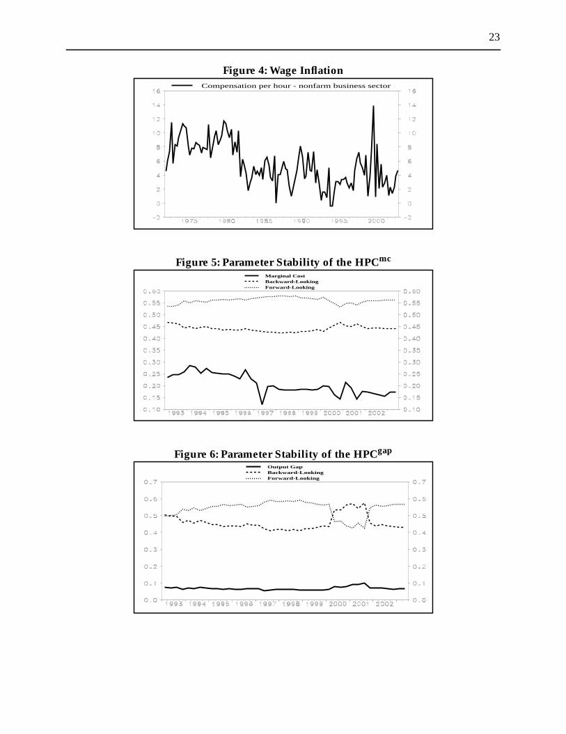
For robustness tests of subsample stability,17 Table 3 reports estimates over the intervals 1972Q
to 1993Q1 and 1979Q3 to 2003Q2. The second interval is associated with the post-Volker p
Results do not appear to vary widely, although the importance of forward-looking behaviou
appears to be greater in the post-Volker period, characterized by low and stable inflation. T
evident from the degree of “backwardness” in price-setting, which declines from a high of 46
cent in the 1972Q2 to 1993Q1 period to a low of 19 per cent in the post-Volker period (both
the output-gap model). The full-sample estimates suggest that, at most, 54 per cent of firm
using backward-looking price-setting rules.
Table 2: Robustness Analysis: Extra Inflation Lagsa
a. The standard error is in parentheses.
Marginal cost Output gap
0.472(0.05)
0.672(0.06)
0.946(0.08)
0.627(0.10)
0.234(0.08)
0.100(0.05)
0.345(0.07)
0.462(0.08)
0.012(0.03)
0.129(0.05)
0.427(0.06)
0.454(0.05)
0.553(0.06)
0.414(0.01)
D 1.89(0.10)
3.05(0.19)
J-statisticb
b. Thep-value is in parentheses.
9.73(0.72)
10.33(0.67)
17. More thorough parametric stability tests are shown in Figures 5 and 6.
β
θ
β
λ
ω
ψ
γb
γ f

10
n
full-
ature.
n of
t for
In addition, marginal costs and the output gap have a significant impact on short-run inflatio
dynamics of approximately the same magnitude as full-sample models. Duration of price
stickiness is estimated to be in the range of 1.9 to 3.1 quarters, not much different from the
sample estimated range of 1.9 to 2.7 quarters.
Estimates of both hybrid Phillips curves are consistent with what has been seen in the liter
As for the PAC model that follows, I tried—without much success—to update the specificatio
both hybrid Phillips curves with the addition of import prices (or the exchange rate) to accoun
the possibility of pass-through to U.S. prices.
Table 3: Robustness Analysis: Subsample Stabilitya
a. The standard error is in parentheses.
Marginal cost Output gap
Parameters 1972Q2–1993Q1 1979Q3–2003Q2(post-Volker)
1972Q2–1993Q1 1979Q3–2003Q2(post-Volker)
0.395(0.04)
0.520(0.06)
0.698(0.06)
0.696(0.03)
1.006(0.04)
0.959(0.03)
0.954(0.05)
0.959(0.02)
0.332(0.10)
0.242(0.11)
0.047(0.02)
0.093(0.02)
0.335(0.04)
0.240(0.07)
0.456(0.06)
0.191(0.05)
0.459(0.03)
0.318(0.05)
0.405(0.05)
0.216(0.05)
0.543(0.04)
0.660(0.05)
0.580(0.04)
0.757(0.03)
D 1.65(0.07)
2.08(0.12)
3.31(0.20)
3.29(0.11)
J-statisticb
b. Thep-value is in parentheses.
8.04(0.84)
8.51(0.81)
8.31(0.82)
6.45(0.93)
θ
β
λ
ω
γb
γ f

11
ided
PAC
st as
zed by
are
and
rice of
e
4. The Polynomial Adjustment-Cost Approach
4.1 The model
An alternative approach to modelling inflation, in the hybrid neo-Keynesian context, is prov
by the PAC model as developed by Tinsley (1993) and Kozicki and Tinsley (2002a, b). In the
framework, a firm must take into account the prospect of delays in future price adjustment, ju
in the basic Calvo model. Consequently, the firm selects a reset price that is best characteri
the weighted average of expected equilibrium prices over future periods, where the weights
the discounted survival probabilities of the current reset price, as demonstrated by Kozicki
Tinsley (2002a). Hence, the log reset price of firms allowed to adjust their prices in periodt is
,
, (17)
whereF is the usual lead operator.
Accordingly, the current aggregate logged price is a geometric average of the current reset p
adjusting firms and the past prices of firms not yet able to adjust their prices,
,
, (18)
whereL is the usual lag operator.
As in Kozicki and Tinsley (2002a), by combining (17) and (18), the dynamic behaviour of th
aggregate price can be defined by the linear difference equation,
. (19)
Adding to both sides of equation (19) yields the following:
. (20)
pr t, Et 1 βθ–( ) βθ( )ipt i+
*
i 0=
∞
∑
=
Et1 βθ–( )
1 βθF–( )------------------------ pt
*
=
pt 1 θ–( ) pr t, θ pr t 1–, θ2pr t 2–, …+ + +[ ]=
1 θ–( )1 θL–( )
-------------------- pr t,=
Et 1 θL–( ) 1 βθF–( ) pt{ } 1 θ–( ) 1 βθ–( ) pt*=
θ 1 β+( ) pt
πt Etβπt 1+1 θ–( ) 1 βθ–( )
θ------------------------------------- pt
* pt–( )+=
12
(20)
in the
ming
al
tated
the
he
n this
).
n the
ption
ithm
s and
The sole difference between the New Keynesian Phillips curve in equation (9) and equation
is that the price gap in the latter, , is represented by marginal cost (or the output gap)
former.18
Hence, following Tinsley (1993), the optimal intertemporal planning can be captured by assu
that firms choose their relative price to minimize per cent deviations from the desired optim
price path subject to frictions on price adjustment. The planning problem therefore can be s
as:
, (21)
where is a cost forecast based on information available at the beginning of periodt, and
is a discount factor. The term is the cost associated with the spread between
actual and desired price level at timet+i, and is the unit cost associated with this spread. T
remainder of this cost function represents an (m-1)-order frictional polynomial that captures
frictions on price adjustment. This planning problem is best described by the PAC approach
developed by Tinsley (1993), and inflation can therefore be described as19:
. (22)
Hence, inflation at timet is subject to three distinctive elements: the spread at timet-1 between the
actual and desired price level, past inflation, and a weighted forecast of expected inflation. I
case, the weights, , are a function of the discount rate ( ) and of the cost parameters (
4.2 Estimates of the PAC model
4.2.1 Cointegration test and desired path
The theoretical framework implies that there must exist a cointegration relationship betwee
desired path variables. The desired price path, measured by the logarithm of core consum
deflator (core PCE), is a function of the logarithm of labour compensation ( ) and the logar
of energy prices ( ), given by:
18. In the spirit of Galí and Gertler (1999), Kozicki and Tinsley (2002a) also argue that marginal costoutput gaps are closely related.
19. This is a variant of what Kozicki and Tinsley (2002b) propose.
pt* pt–
minp Et βi κ0 pt i+ pt i+
*–( )2
κ1 ∆ pt i+( )2 κ2 ∆2pt i+( )
2κ3 ∆3
pt i+( )2
...+ + + +[ ]i 0=
∞
∑
Et .{ } βpt i+ pt i+
*–( )2
κ0
πt a0 Pt 1– Pt 1–*
–( ) ajπt j–j 1=
m 1–
∑+– Et 1– f iπt i– 1+i 0=
∞
∑
+=
f i β κi
lw
lener

13
sselin
I
del
d by
3Q2.
th
et al.
tothe
ions.
, (23)
where is the trend labour productivity in the non-farm business sector as estimated by Go
and Lalonde (2002). This specification is much in line with what has been estimated in the
FRB/US macroeconomic model.20 To test for cointegration among the desired path variables,
adopt Johansen’s procedure.21 The Hannan-Quinn and Shwartz criteria determine that the mo
should include four lags. Results show that the null hypothesis of no cointegration is rejecte
the data (Table 4).
Given the simultaneity problem, the desired price path (23) is estimated via a non-linear
instrumental variables (GMM) estimator on a quarterly basis over the period 1972Q2 to 200
The GMM is instrumented using four lags of each variable included in the desired price-pa
equation (23).22 Estimation results are reported in Table 5.23,24
20. Equations in the FRB/US model are described in Brayton and Tinsley (1996) and Brayton(1997).
21. Unit-root testing reveals that all variables are integrated of order 1.
Table 4: Johansen Cointegration Testa
a. The null hypothesis is rejected if the computed value is greater than the critical one.
Cointegrating space PGp Critical valueb
b. Threshold of 10 per cent.
Prices, labour compensation, andenergy prices
44.04 32.00
22. Results are not sensitive to the number of lags.23. Figures 7 and 8 show the evolution of the observed and desired price path.24. The coefficients on labour compensation (adjusted for productivity) and energy prices can be
interpreted as the cointegrating vector of the system. A common, though incorrect, inclination isgive an interpretation to the cointegrating vector coefficients. However, one cannot assume thatcoefficients in the cointegrating vector represent partial derivatives. Wickens (1996) shows thatreduced-form cointegrating vectors should not be interpreted without further structural assumptIntuitively, given the endogeneity that characterizes the set of variables, a shock to each variableinduces movements in the others.
pt* α0 α+ 1lenert α2 lwt ρt–( )+=
ρt

14
1 to
y test,
he
red
ch of
tion
ce
e price
To account for the highly unusual period of stock market returns that stretched from 1999Q
2003Q2, I also estimate the model over the period 1972Q2 to 1998Q4.25 This period did not
affect the estimates of the desired price path. To provide a more thorough parametric stabilit
I perform rolling estimations of the desired path coefficients over the period 1993 to 2003. T
parameters are highly stable, as confirmed in Figure 9.
4.2.2 Dynamic equation
Prior to estimating the dynamic equation for the inflation PAC, we need to forecast the desi
price path. We use a “satellite” VAR to do so. This small model encompasses four lags of ea
the variables included in the desired price path: prices, labour compensation (adjusted for
productivity), and energy prices.
The order of the PAC must also be predetermined. Preliminary results suggest that the infla
PAC is of order m = 4 in equation (22).26 This result is in line with the dynamic inflation equation
in the FRB/US model. With m = 4, it appears to be costly for firms to adjust the first four pri
moments.27
In addition to the usual explanatory variables, I include a moving average of four lags of the
output gap and one lag of inflation in import prices in the PAC specification (equation (24)).
25. This is in the spirit of Gosselin and Lalonde (2002).
Table 5: Desired Price Path
1972Q4–2003Q1a
a. The p-value is in parentheses.
1972Q4–1998Q4
Constant-3.93(0.00)
-3.88(0.00)
Labour compensation(adjusted for productivity)
1.26(0.00)
1.25(0.00)
Energy prices-0.11(0.00)
-0.11(0.00)
26. This empirical choice is dictated by the absence of residual autocorrelation and by the level ofsignificance in the maximum lag.
27. The first three moments can be identified as the level, the growth rate, and the acceleration of thvariable.

15
U.S.
of the
the
een
. As
ly
r cent
.
ng,
ct.
eters
nsitive
is
of the
ions
le 6).
e the
ay to
ables
ssful.
Import prices expressed in domestic currency can offer a proxy for pass-through effects on the
economy.28 To ensure model convergence, I constrain the sum of the coefficients on the lags
dependent variable and the expectation term to 1:
. (24)
To circumvent the potential simultaneity problem, I estimate the dynamic equation of the PAC
specification through GMM. I instrument the model using four lags of inflation, labour
compensation, and energy prices. Table 6 shows the results.
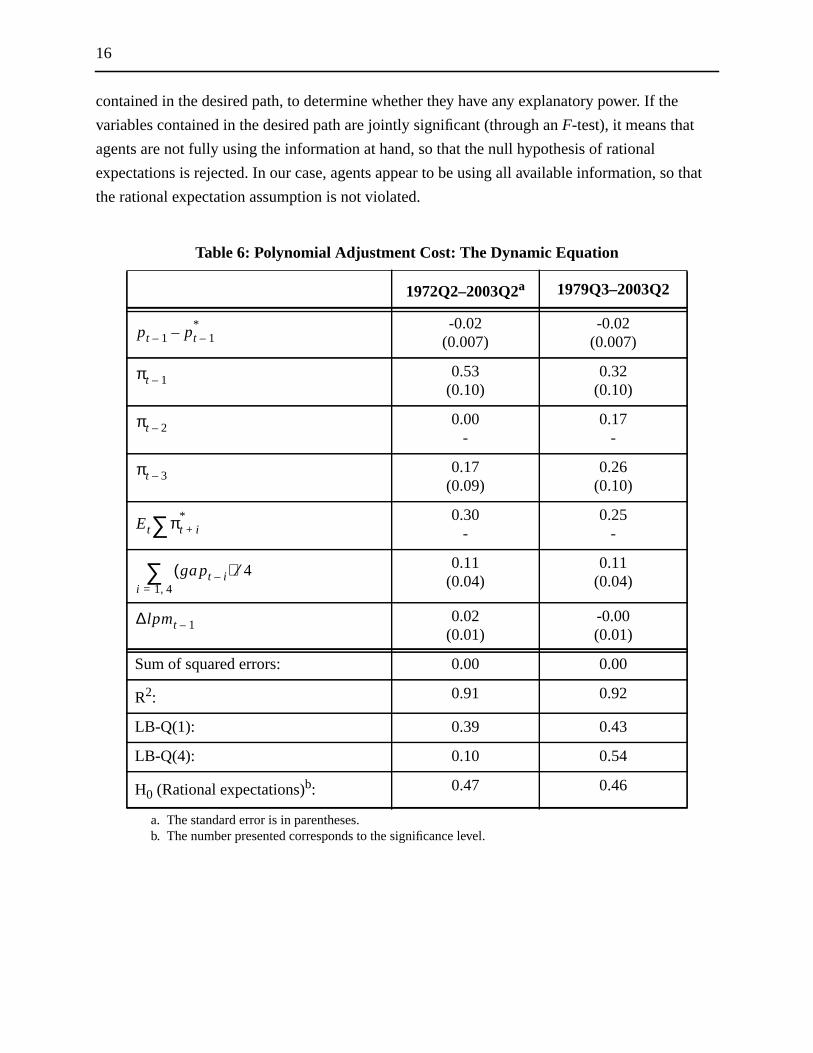
The model’s R2 is fairly high at 91 per cent and the residuals are white noise, as confirmed by
Ljung-Box Q test (significance level of 0.39). The coefficient on the error-correction term betw
the observed and desired price path is in the order of -0.02, compared with -0.07 in FRB/US
expected, given the observed persistence in inflation, adjustment costs appear to be relative
important. The price level converges to its desired path at a rate of 2 per cent per quarter (8 pe
annually). The sum of the coefficients associated with the lagged dependent variable is 0.70
Correspondingly, the sum of the forward-looking weights is equal to 0.30. This is not surprisi
given the observed persistence of the inflation process.29 As expected, the coefficient on import
prices (0.02) is positive for the full sample, denoting a small but significant pass-through effe
For the hybrid Phillips curve models, subsample stability was considered. I tried to gauge the
parameter stability over the intervals 1972Q2 to 1993Q1 and 1979Q3 to 2003Q2. The param
appear to be stable. The coefficient associated with import prices, however, appears to be se
to the sample selection, and quickly falls out of the equation when a more recent subsample
considered, which suggests a negligible pass-through for the U.S. economy in the latter part
sample.30 Figure 10 shows a more thorough parametric stability test. I perform rolling estimat
of the dynamic PAC specification over the period 1993 to 2003. Although the expectations
parameter appears to decline over time, the parameters appear to be stable.
Following Gosselin and Lalonde (2003), I test the null hypothesis of rational expectations (Tab
This procedure examines the underlying assumption that expectations are formed to minimiz
root mean-squared error (RMSE) of the forecast, conditional on the set of information. One w
verify this assumption is to regress the residual of the PAC model on the growth rate of the vari
28. The inclusion of import prices (or the exchange rate) in the Galí and Gertler framework is not succe29. The weight distribution has been calculated and is presented in Figure 11.30. This is consistent with the recent pass-through trend.
πt a0 Pt 1– Pt 1–*
–( ) ajπt j–j 1=
m 1–
∑+– Et 1– f iπt i– 1+i 0=
∞
∑
λ1 gapt j–j 1 4,=∑ λ2lpmt+ + +=
16
e
o that
contained in the desired path, to determine whether they have any explanatory power. If th
variables contained in the desired path are jointly significant (through anF-test), it means that
agents are not fully using the information at hand, so that the null hypothesis of rational
expectations is rejected. In our case, agents appear to be using all available information, s
the rational expectation assumption is not violated.
Table 6: Polynomial Adjustment Cost: The Dynamic Equation
1972Q2–2003Q2a
a. The standard error is in parentheses.
1979Q3–2003Q2
-0.02(0.007)
-0.02(0.007)
0.53(0.10)
0.32(0.10)
0.00-
0.17-
0.17(0.09)
0.26(0.10)
0.30-
0.25-
0.11(0.04)
0.11(0.04)
0.02(0.01)
-0.00(0.01)
Sum of squared errors: 0.00 0.00
R2: 0.91 0.92
LB-Q(1): 0.39 0.43
LB-Q(4): 0.10 0.54
H0 (Rational expectations)b:
b. The number presented corresponds to the significance level.
0.47 0.46
pt 1– pt 1–*
–
πt 1–
πt 2–
πt 3–
Et πt i+*∑
gapt i–( ) 4⁄i 1 4,=∑
∆lpmt 1–

17
d-
7
Es of
the
gests
o
thesis
the
odels.
5. Forecasting Inflation: A Look at Competing Approaches for theUnited States
In this section, I evaluate the forecasting properties of the inflation models. Out-of-sample
forecasts are obtained for the period 1993Q1 to 2003Q2.31 This exercise assumes that the
forward-looking components in all specifications are exogenous to the systems (i.e., forwar
looking variables are known with certainty at any given timet). I compare the forecasts of all the
different specifications at different horizons to determine which model performs best. Table
reports the RMSE results. It appears, at the margin, that the HPCgap is the best-performing
forecasting model. The Diebold-Mariano test, which tests the null hypothesis that the RMS
competing models are statistically identical, reveals that the performance of the HPCgap
specification is better than that of the HPCmc, and statistically as good as that of the alternative
PAC model.
Table 8 reports thep-value for the out-of-sample encompassing tests between the different
models. I test the null hypothesis that it is possible to improve the forecast of a model using
forecast of an alternative model. In most instances, the null hypothesis is rejected, which sug
that none of the competing models can improve the forecast of alternative models. There d
appear to be a few interesting exceptions. First and foremost, the test cannot reject the hypo
that the HPCgapforecast improves on the HPCmc forecast, which suggests that the HPCgapmodel
performs better than its HPCmc counterpart. It would also seem that the HPCgap model improves
the PAC model over short periods. Correspondingly, I cannot reject the null hypothesis that
31. Figures 12, 13, and 14 show the one-, four-, and eight-step-ahead forecasts for the competing m
Table 7: Root Mean-Squared Error (1993Q1–2003Q2)a
a. The Diebold-Mariano test rejects the null hypothesis that the RMSEs of competingmodels are statistically identical at 1 per cent (*), 5 per cent (**), and 10 per cent(***).
N-step-aheadforecast with N = HPCgap HPCmc PAC
One 0.0016 0.0018*** 0.0018
Two 0.0017 0.0020 0.0020
Four 0.0017 0.0021** 0.0022
Eight 0.0017 0.0026* 0.0020

18
h
e
king
he
uld be
the
one-step-ahead PAC forecast improves that of the HPCmc model at the 10 per cent confidence
level. The HPCmc forecast, however, improves the PAC forecast over the same horizon, whic
suggests that the two forecasts do not embed the same information. It would appear that th
HPCgap model performs marginally better than the other two specifications.
6. Conclusion
The New Keynesian Phillips curve is theoretically appealing, because its purely forward-loo
specification is based on a model of optimal pricing behaviour with rational expectations. T
observed persistence in inflation, however, suggests that lags as well as leads of inflation wo
required in an appropriate empirical specification. The hybrid Phillips curve, which includes
Table 8: Encompassing Tests (p-values)
Null hypothesis
N-step-aheadforecast with
N =
PAC improves HPCmc PAC improves HPCgap
One 0.13 0.00
Two 0.02 0.00
Four 0.00 0.00
Eight 0.00 0.00
HPCmc improves PAC HPCmc improves HPCgap
One 0.15 0.01
Two 0.03 0.00
Four 0.00 0.00
Eight 0.00 0.00
HPCgap improves HPCmc HPCgap improves PAC
One 0.88 0.14
Two 0.77 0.02
Three 0.57 0.00
Four 0.27 0.00

19
f lags
are
quite
ost
f the
low
ture
nship is
ough
output gap as an explanatory variable, seeks to justify, on the basis of theory, the addition o
in the New Keynesian Phillips curve. I have shown that the resulting forecast performances
marginally better than those of alternative model specifications (HPCmc and PAC), without losing
theoretical consistency, which is central to monetary policy-making.
Nevertheless, a few caveats remain. First, the degree of forward-lookingness appears to be
sensitive to the sample selection. As I truncate the sample window to account for only the m
recent history, the behaviour of agents becomes more forward looking, possibly because o
U.S. monetary authority’s growing credibility, given its success in achieving and maintaining
and stable inflation.
It is difficult to estimate a significant relationship between inflation and import prices (or the
exchange rate). This difficulty could potentially be attributed to the comparatively closed na
of the U.S. economy. It could also be the case, however, that the absence of such a relatio
not totally unexpected, since the inflation dynamic can ultimately be described in terms of a
discounted stream of future output gaps, which would normally include all available pass-thr
information.

20
ew
ed
.
inal
tary
P.”
éric-
-
k of
References
Blinder, A.S., E.R.D. Canetti, D.E. Lebow, and J.B. Rudd. 1998. “Asking About Prices: A NApproach to Understanding Price Stickiness.” New York: Russell Sage Foundation.
Brayton, F. and P. Tinsley. 1996. “A Guide to FRB/US: A Macroeconomic Model of the UnitStates.” Federal Reserve Board, FEDS Working Paper No. 1996-42.
Brayton, F., E. Mauskopf, D. Refschneider, P. Tinsley, and J. Williams. 1997. “The Role ofExpectations in the FRB/US Macroeconomic Model.”Federal Reserve Bulletin (April):227–45.
Calvo, G. 1983. “Staggered Prices in a Utility-Maximizing Framework.”Journal of MonetaryEconomics 12: 383–98.
Carlton, D. 1986. “The Rigidity of Prices.”American Economic Review (September): 637–58.
Christiano, L., M. Eichenbaum, and C. Evans. 1997. “Sticky Price and Limited ParticipationModels: A Comparison.”European Economic Review 41: 1201–49.
Cooley, T.F. and E. Prescott. 1995. “Economic Growth and Business Cycles.” InFrontiers ofBusiness Cycle Research, edited by T.F. Cooley. Princeton: Princeton University Press
Dixit, A. and J. Stiglitz. 1977. “Monopolistic Competition and Optimum Product Diversity.”American Economic Review (June): 297–308.
Fuhrer, J. and G. Moore. 1995. “Monetary Policy Tradeoffs and the Correlation between NomInterest Rates and Real Output.”American Economic Review (March): 219–39.
Galí, J. and M. Gertler. 1999. “Inflation Dynamics: A Structural Econometric Analysis.”Journalof Monetary Economics 44: 195–222.
Galí, J., M. Gertler, and J.D. Lopez-Salido. 2001. “European Inflation Dynamics.”European Eco-nomic Review 45: 1237–70.
Goodfriend, M. and R. King. 1997. “The New Neoclassical Synthesis and the Role of MonePolicy.” In NBERMacroeconomics Annual, edited by B. Bernanke and J. Rotemberg,231–83. Cambridge, MA: MIT Press.
Gosselin, M.-A. and R. Lalonde. 2002. “An Eclectic Approach to Estimating U.S. Potential GDBank of Canada Working Paper No. 2002-36.
———. 2003. “Un modèle ‘PAC’ d’analyse et de prévision des dépenses des ménages amains.” Bank of Canada Working Paper No. 2003-13.
King, R.G. and A.L. Wolman. 1996. “Inflation Targeting in a St. Louis Model of the 21st Century.” NBER Working Paper No. 5507.
Kozicki, S. and P.A. Tinsley. 2002a. “Dynamic Specifications in Optimizing Trend-DeviationMacro Models.”Journal of Economic Dynamics and Control 26: 1585–1611.
———. 2002b. “Alternative Sources of the Lag Dynamics of Inflation.” Federal Reserve BanKansas City Working Paper No. 02-12.
21
ch.”
roard
Rennison, A. 2003. “Comparing Alternative Output-Gap Estimators: A Monte Carlo ApproaBank of Canada Working Paper No. 2003-8.
Rotemberg, J.J. 1982. “Sticky Prices in the United States.”Journal of Political Economy 90:1187–1211.
Sbordone, A. 2002. “Prices and Unit Labor Costs: A New Test of Price Stickiness.”Journal ofMonetary Economics 49-2 (March): 265–92.
Tinsley, P.A. 1993. “Fitting Both Data and Theories: Polynomial Adjustment Costs and ErroCorrection Decision Rules.” Finance and Economic Discussion Series No. 1993-21, Bof Governors of the Federal Reserve System.
Wickens, M. 1996. “Interpreting Cointegrating Vector and Common Stochastic Trends.”Journalof Econometrics74: 255–71.
Woodford, M. 1996. “Control of the Public Debt: A Requirement for Price Stability?” NBERWorking Paper No. 5684.

22
Figure 1: Personal Consumption Expenditure Inflation
Figure 2: Output Gap
Figure 3: Marginal Cost
Core indexTotal index
Adjusted labour share
23
Figure 4: Wage Inflation
Figure 5: Parameter Stability of the HPCmc
Figure 6: Parameter Stability of the HPCgap
Compensation per hour - nonfarm business sector
Marginal CostBackward-LookingForward-Looking
Output GapBackward-LookingForward-Looking

24
Figure 7: Observed and Desired Price Path
Figure 8: Gap Between the Observed and Desired Price Path
Figure 9: Parameter Stability of the Desired Price PathConstantWagesEnergy prices

25
Figure 10: Parameter Stability of the Dynamic PAC Equation
Figure 11: Decomposition of the Expectation Term
Figure 12: Forecasting Properties: One-Step-Ahead
DisequilibriumDiscounted output gapExpectationsImport prices
Observed inflationHPC-GapHPC-mcPAC

26
Figure 13: Forecasting Properties: Four-Steps-Ahead
Figure 14: Forecasting Properties: Eight-Steps-Ahead
Observed inflationHPC-GapHPC-mcPAC
Observed inflationHPC-GapHPC-mcPAC
27
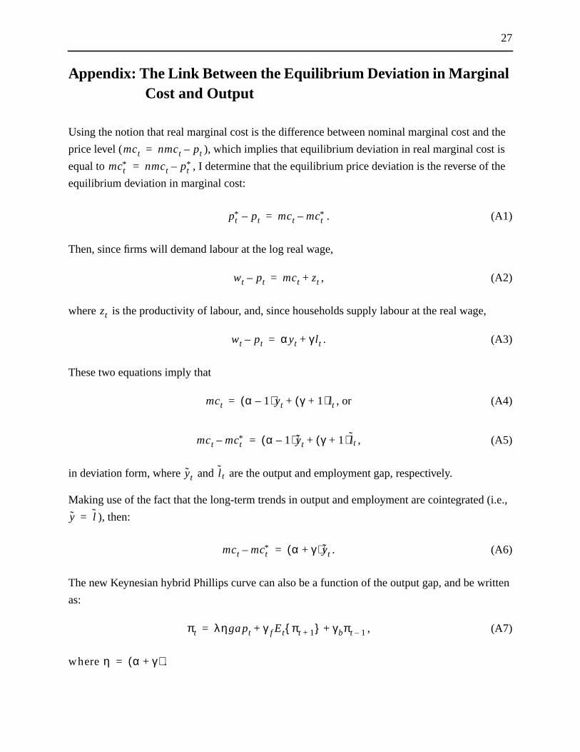
Appendix: The Link Between the Equilibrium Deviation in MarginalCost and Output
Using the notion that real marginal cost is the difference between nominal marginal cost and the
price level ( ), which implies that equilibrium deviation in real marginal cost is
equal to , I determine that the equilibrium price deviation is the reverse of the
equilibrium deviation in marginal cost:
. (A1)
Then, since firms will demand labour at the log real wage,
, (A2)
where is the productivity of labour, and, since households supply labour at the real wage,
. (A3)
These two equations imply that
, or (A4)
, (A5)
in deviation form, where and are the output and employment gap, respectively.
Making use of the fact that the long-term trends in output and employment are cointegrated (i.e.,
), then:
. (A6)
The new Keynesian hybrid Phillips curve can also be a function of the output gap, and be written
as:
, (A7)
where .
mct nmct pt–=
mct* nmct pt
*–=
pt* pt– mct mct
*–=
wt pt– mct zt+=
zt
wt pt– αyt γ l t+=
mct α 1–( )yt γ 1+( )l t+=
mct mct*– α 1–( ) yt γ 1+( ) l t+=
yt l t
y l=
mct mct*– α γ+( ) yt=
πt ληgapt γ f Et πt 1+{ } γbπt 1–+ +=
η α γ+( )=

Bank of Canada Working PapersDocuments de travail de la Banque du Canada
Working papers are generally published in the language of the author, with an abstract in both officiallanguages.Les documents de travail sont publiés généralement dans la langue utilisée par les auteurs; ils sontcependant précédés d’un résumé bilingue.
Copies and a complete list of working papers are available from:Pour obtenir des exemplaires et une liste complète des documents de travail, prière de s’adresser à:
Publications Distribution, Bank of Canada Diffusion des publications, Banque du Canada234 Wellington Street, Ottawa, Ontario K1A 0G9 234, rue Wellington, Ottawa (Ontario) K1A 0G9E-mail: [email protected] Adresse électronique : [email protected] site: http://www.bankofcanada.ca Site Web : http://www.banqueducanada.ca
20042004-30 The New Basel Capital Accord and the Cyclical
Behaviour of Bank Capital M. Illing and G. Paulin
2004-29 Uninsurable Investment Risks C. Meh and V. Quadrini
2004-28 Monetary and Fiscal Policies in Canada: Some InterestingPrinciples for EMU? V. Traclet
2004-27 Financial Market Imperfection, Overinvestment,and Speculative Precaution C. Calmès
2004-26 Regulatory Changes and Financial Structure: TheCase of Canada C. Calmès
2004-25 Money Demand and Economic Uncertainty J. Atta-Mensah
2004-24 Competition in Banking: A Review of the Literature C.A. Northcott
2004-23 Convergence of Government Bond Yields in the Euro Zone:The Role of Policy Harmonization D. Côté and C. Graham
2004-22 Financial Conditions Indexes for Canada C. Gauthier, C. Graham, and Y. Liu
2004-21 Exchange Rate Pass-Through and the Inflation Environmentin Industrialized Countries: An Empirical Investigation J. Bailliu and E. Fujii
2004-20 Commodity-Linked Bonds: A Potential Means forLess-Developed Countries to Raise Foreign Capital J. Atta-Mensah
2004-19 Translog ou Cobb-Douglas? Le rôle des duréesd’utilisation des facteurs E. Heyer, F. Pelgrin, and A. Sylvain
2004-18 When Bad Things Happen to Good Banks:Contagious Bank Runs and Currency Crises R. Solomon
2004-17 International Cross-Listing and the Bonding Hypothesis M. King and D. Segal
2004-16 The Effect of Economic News on Bond Market Liquidity C. D’Souza and C. Gaa
2004-15 The Bank of Canada’s Business OutlookSurvey: An Assessment M. Martin and C. Papile