The new GFDL global atmosphere and land model AM2/LM2:

Evaluation with prescribed SST simulations

GFDL’s Global Atmospheric Model Development Team (GAMDT)

Jeffrey L. Anderson+, V. Balaji&, Anthony J. Broccoli+^, William F. Cooke%,

Thomas L. Delworth+, Keith W. Dixon+, Leo J. Donner+, Krista A. Dunne#,

Stuart M. Freidenreich+, Stephen T. Garner+, Richard G. Gudgel+, C. T. Gordon+,

Isaac M. Held+, Richard S. Hemler+, Larry W. Horowitz+, Stephen A. Klein+*,

Thomas R. Knutson+, Paul J. Kushner+*, Amy R. Langenhorst%, Ngar-Cheung Lau+, Zhi Liang%,

Sergey L. Malyshev@, P. C. D. Milly#, Mary J. Nath+, Jeffrey J. Ploshay+, V. Ramaswamy+,

M. Daniel Schwarzkopf+, Elena Shevliakova@, Joseph J. Sirutis+, Brian J. Soden+, William F. Stern+,

Lori A. Thompson%, R. John Wilson+, Andrew T. Wittenberg$, and Bruce L. Wyman+

+Geophysical Fluid Dynamics LaboratoryNational Oceanic and Atmospheric Administration

Princeton, New Jersey

&Silicon Graphics IncorporatedPrinceton, New Jersey

%RSISMcLean, Virginia,presently at GFDL

#U.S. Geological SurveyPrinceton, New Jersey

$Atmospheric and Oceanic Sciences Visiting Scientists ProgramPrinceton University

Princeton, New Jersey

@Department of Ecology and Evolutionary BiologyPrinceton University

Princeton, New Jersey

Submitted to Journal of Climate, March 2003

___________________________________________________________________________________*Corresponding authors and team leaders: Stephen A. Klein and Paul J. Kushner, Geophysical FluidDynamics Laboratory/NOAA, Princeton University Forrestal Campus/ US Route 1, P.O.Box 308, Princ-eton, New Jersey 08542, e-mail: Stephen.Klein@gfdl.noaa.gov and Paul.Kushner@gfdl.noaa.gov

^Now at Department of Environmental Sciences, Rutgers University, New Brunswick, New Jersey.

Abstract

The configuration and performance of a new global atmosphere and land model developed

at the Geophysical Fluid Dynamics Laboratory (GFDL) for climate research is presented. The

atmosphere model, known as AM2, includes a new gridpoint dynamical core, a prognostic cloud

scheme, and a multi-species aerosol climatology, as well as components from previous models

used at GFDL. The land model, known as LM2, includes soil heat storage, groundwater storage,

and stomatal effects. The performance of the coupled model AM2/LM2 is evaluated with a series

of prescribed sea-surface temperature (SST) simulations. Particular focus is given to the model’s

climatology and the characteristics of interannual variability related to El Niño/Southern Oscilla-

tion (ENSO).

One of the integrations was performed according to the prescriptions of the second

Atmospheric Model Intercomparison Project (AMIP II) and data were submitted to the Program

for Climate Model Diagnosis and Intercomparison (PCMDI). Particular strengths of AM2/LM2,

as judged by comparison to other models participating in AMIP II, include a commendable simu-

lation of the shortwave radiation budget and temperatures in the extratropical lower stratosphere

near 200 hPa. Distinct weaknesses of AM2/LM2, as compared to other AMIP II models, include

midlatitude oceanic westerly wind stresses that are shifted equatorward and a tendency towards a

double Intertropical Convergence Zone (ITCZ) in the Pacific. Other prominent problems include

unrealistically weak tropical transient activity, a positive Arctic sea level pressure (SLP) bias, and

excessive wintertime cloudiness over high latitude continents.

An ensemble of 10 integrations with observed SSTs for the second half of the twentieth

century permits a statistically reliable assessment of the model’s response to ENSO. Although the

model produces credible precipitation anomalies in the tropical Pacific and Asian sectors, the

response of the geopotential height in the North Pacific and North American sector is unrealisti-

cally weak.

GFDL GAMDT

1

1. Introduction

In this report, an overview is presented of the new GFDL global atmosphere and land

model known as "AM2/LM2". AM2 and LM2 are, respectively, the atmospheric and terrestrial

components of the earth-system model that is under development at GFDL for climate research

and climate prediction applications. In developing AM2/LM2, the focus has been on consolidat-

ing and improving the various versions of such models that have been used in GFDL’s past (Ham-

ilton et al. 1995, Stern and Miyakoda 1995, Delworth et al. 2002). The principal aim is to create a

model that represents realistically the dynamic, thermodynamic, and radiative characteristics of

the climate system and is suitable for coupling to ocean and sea-ice models without flux adjust-

ment. Balanced against this aim is the need to have a model computationally fast enough so that

ensemble multi-century integrations may be performed.

Although AM2/LM2 incorporates many important pieces of previous models used within

GFDL, it does represent a substantial break from the past. AM2 includes a new gridpoint atmos-

pheric dynamical core, a multi-species three dimensional aerosol climatology, and a fully prog-

nostic cloud scheme. LM2 incorporates soil heat storage, groundwater storage, stomatal control of

transpiration, and soil and plant dependent parameters. These new components have required

modification and retuning of those pieces of the components that were carried over from previous

models. This has led to a model with more capabilities and potential for growth as well as a model

with simulation characteristics generally superior to that of the older GFDL models.

Our model development effort is team-based and involves a broad cross section of exper-

tise from within and outside of GFDL; this has required a challenging degree of coordination. A

GFDL GAMDT

2

simultaneous challenge has been GFDL’s transition from vector to parallel computing architec-

tures. To address these challenges, an in-house software framework known as the "Flexible Mod-

eling System" (FMS, http://www.gfdl.noaa.gov/~fms) has been developed. FMS based codes are

modular, use Fortran 90, and are based on standardized interfaces between component models

(i.e. land, atmosphere, ocean, sea-ice). The software conservatively passes the fluxes of heat,

moisture, and momentum between component models which may have different horizontal grids.

The FMS code organization isolates those aspects of the code related to parallel computing to a

relatively simple message passing interface (http://www.gfdl.noaa.gov/~vb/mpp.html). As a

result, scientists developing new code for the model need not learn the intricacies of parallel com-

puting. Using the FMS, it has been possible to rapidly test a variety of model configurations and

follow parallel development paths for the atmosphere, ocean, land, and sea-ice models. FMS

models have been tested simultaneously on vector and parallel platforms. As a consequence, the

transition to a new parallel computing environment was made with relative ease.

Section 2 of the report documents the components of AM2/LM2 as well as the boundary

conditions for the experiments performed. Section 3 provides a discussion of AM2/LM2’s clima-

tological circulation, hydrology and radiation budget, as well as its variability. A brief comparison

of the quality of AM2/LM2’s climatology to that of other models is given in section 4 while future

plans are discussed in section 5.

2. Model components and boundary conditions

The components of AM2/LM2 are described in the following three subsections. For ease

of reference, a summary of model components is given in Table 1.

GFDL GAMDT

3

a. Grid-point dynamical core

The hydrostatic, finite difference dynamical core has been developed from models

described in Mesinger et al. (1988) and Wyman (1996). The AM2/LM2 dynamical core solves the

equations for the same set of prognostic variables as in these references, but uses a different hori-

zontal and vertical grid. The latitude-longitude horizontal grid is the staggered Arakawa B-grid

(Arakawa and Lamb 1977) with resolution 2.5˚ longitude by 2˚ latitude. In the vertical, a hybrid

coordinate grid is used; sigma surfaces near the ground continuously transform to pressure sur-

faces above 250 hPa (Table 2). The model has 18 vertical levels with the lowest model level about

30 meters above the surface. Five levels are in the stratosphere with the top level at about 3 hPa.

The prognostic variables are the zonal and meridional wind components, surface pressure, tem-

perature, and tracers. The tracers include specific humidity and three prognostic cloud variables

(section 2b3).

The model utilizes a two-level time differencing scheme. Gravity waves are integrated

using the forward-backward scheme (Mesinger 1977) and a split time differencing scheme is used

for longer advective and physics time steps (Gadd 1978). The advective terms are integrated with

a modified Euler backward scheme that has less damping than the full backward scheme (Kuri-

hara and Tripoli 1976). Note that the Euler backward scheme is needed for stability. The gravity

wave, advective and physics time steps are 200, 600, and 1800 seconds, respectively.

The energy and angular momentum conserving vertical finite difference scheme used is

from Simmons and Burridge (1981). Horizontal advection uses centered spatial differencing.

Momentum advection is fourth-order; temperature and tracer advection is second-order. The ver-

tical advection of tracers use a piecewise linear finite volume scheme (Lin et al. 1994). Grid point

GFDL GAMDT

4

noise and the 2∆x computational mode of the B-grid are controlled with linear fourth-order hori-

zontal diffusion. A term is added to the diffusive fluxes of heat and moisture to prevent spurious

diffusion up sloping model surfaces. A second order Shapiro (1970) filter is applied to the depar-

tures from the zonal mean of the zonal wind component and to the total meridional wind compo-

nent at the top model level to reduce the reflection of waves. Fourier filtering is applied poleward

of 60˚ latitude to damp the shortest resolvable waves so that a longer time step can be taken. The

filter is applied to the mass divergence, the horizontal omega-alpha term, the horizontal advective

tendencies, and the momentum components.

Excluding the dissipation terms and time differencing, the numerical schemes are

designed to conserve total energy. To guarantee energy conservation for long climate runs, a glo-

bal energy correction is applied to temperature.

b. Atmospheric physics

1) RADIATION AND PRESCRIBED OZONE AND AEROSOL CLIMATOLOGIES

The shortwave radiation algorithm follows Freidenreich and Ramaswamy (1999; hereinaf-

ter FR99), with the following modifications. With a view towards computational efficiency, the

band structure and the number of exponential-sum fit terms within some bands have been altered,

resulting in fewer pseudo-monochromatic columnar calculations. Specifically, the band from 0-

2500 cm-1 now has one instead of six terms, owing to consideration of CO2 as the only absorber

for this interval; there is one band from 2500-4200 cm-1 instead of three, and the total number of

terms is reduced from twelve to eight; there is one band from 4200 to 8200 cm-1 instead of four,

and the total number of terms is reduced from twenty-four to nine; the number of terms for the

GFDL GAMDT

5

8200-11500 cm-1 band is reduced from seven to five while that for the 11500-14600 cm-1 band is

reduced from eight to two; there are three bands between 27500 and 34500 cm-1 (viz., 27500 to

32400, 32400 to 33300 and 33300 to 34500) instead of five, each with one term. The number of

bands in the solar spectrum is reduced from twenty-five to eighteen, while the total pseudo-mono-

chromatic column calculations required per grid-box is reduced from seventy-two to thirty-eight.

The new band structure and the revised exponential-sum fits have been developed and tested using

the ’benchmark’ calculations described in FR99. The maximum error in the clear-sky heating

rates is about 15%, a moderate increase from the less than 10% error obtained with the seventy-

two-term fit. The errors in the shortwave overcast sky heating rates for the water cloud model con-

sidered (Slingo 1989) are now ~15%, increased from ~10% for the 72-term fit; for ice clouds, the

errors tend to be larger (FR99) and for the present parameterization could reach ~25%.

The interactions considered include absorption by H2O, CO2, O3, O2, molecular scattering,

and absorption and scattering by aerosols and clouds. For water clouds, the single-scattering prop-

erties in the solar spectrum follow Slingo (1989); for ice clouds, the formulation follows Fu and

Liou (1993). Three-dimensional, monthly-mean profiles of aerosol mass concentrations and their

optical properties follow Haywood et al. (1999) and Haywood (personal communication). The

prescription accounts for sea-salt (low windspeed case) and the natural and anthropogenic compo-

nents of dust, carbonaceous (black and organic carbon) aerosol, and sulfate.

Ozone profiles follow Fortuin and Kelder (1998) and are based on observations over the

1989-1991 period. This climatology has been shown to yield results that represent substantial

improvements over those obtained with previous older climatologies used in the GFDL global

models (Ramaswamy and Schwarzkopf 2002).

GFDL GAMDT

6

The ocean surface is assumed to be Lambertian, with the albedo being a function of the

solar zenith angle following the formulation of Taylor et al. (1996).

The band-averaging of the single-scattering parameters is performed using the thick-aver-

aging technique (Edwards and Slingo 1996). The delta-Eddington technique is employed to com-

pute the layer reflection and transmission based on the single-scattering properties of that layer

(FR99). The diffuse incident beam is assumed to be isotropic and its reflection and transmission is

computed using an effective angle of 53˚, in contrast to the 4-point quadrature scheme in FR99.

The net direct and diffuse quantities in each layer is given by the weighted sum of the clear and

overcast sky fractions present in that layer. The fluxes and heating rates are computed using an

"adding" scheme (Ramaswamy and Bowen 1994).

The longwave radiation code follows the modified form of the Simplified Exchange

Approximation and is also developed and tested using ‘benchmark’ computations (Schwarzkopf

and Ramaswamy 1999). It accounts for the absorption and emission by the principal gases in the

atmosphere, including H2O, CO2, O3, N2O, CH4, and the halocarbons CFC-11, CFC-12, CFC-113

and HCFC-22. For the water vapor continuum, the CKD 2.1 formulation of Clough et al. (1992) is

used. Aerosols and clouds are treated as absorbers in the longwave, with non-grey absorption

coefficients specified in the eight spectral bands of the transfer scheme, following the methodol-

ogy adopted in Ramachandran et al. (2000). For water clouds, the absorption coefficients follow

those employed in Held et al. (1993) while, for ice, the Fu and Liou (1993) prescription is used.

2) CUMULUS PARAMETERIZATION

Moist convection is represented by the Relaxed Arakawa-Schubert (RAS) formulation of

GFDL GAMDT

7

Moorthi and Suarez (1992), with the following modifications. (a) The fraction of water condensed

in the cumulus updrafts which becomes precipitation (known as the ’precipitation efficiency’) is

specified to be 0.986 for deep convection and 0.1 for shallow convection. Deep convection is

defined as updrafts which detrain at pressure levels above 500 hPa whereas shallow convection is

defined as updrafts which detrain beneath 800 hPa. For pressures between 500 and 800 hPa, the

precipitation efficiency is linearly interpolated in pressure between the values for deep and shal-

low convection. Note that this version of RAS lacks cumulus updraft microphysics such as that

developed by Sud and Walker (1999). (b) The non-precipitated fraction of condensed water, 0.014

for deep convection and 0.9 for shallow convection, is a source of condensate for the prognostic

cloud scheme. (c) Re-evaporation of convective precipitation is allowed to occur. Note that this

version of RAS does not include the effects of convective downdrafts developed by Moorthi and

Suarez (1999) in a later version. (d) The time scale over which the cloud work function is relaxed

to a cloud type dependent value is modified so that deep updrafts relax over a time scale of about

12 hours but shallow updrafts relax over a time scale of only 2 hours. (e) The cloud type depend-

ent cloud work function is based upon observations (Lord and Arakawa 1980) but enhanced by

40% to encourage increased tropical transient activity.

3) CLOUD SCHEME

Large-scale clouds are parameterized with separate prognostic variables for the liquid and

ice specific humidities. Cloud fraction is also treated as a prognostic variable of the model follow-

ing the parameterization of Tiedtke (1993). Cloud microphysics are parameterized according to

Rotstayn (1997) with an updated treatment of mixed phase clouds (Rotstayn et al. 2000). Fluxes

of large-scale rain and snow are diagnosed and the amount of precipitation flux inside and outside

GFDL GAMDT

8

of clouds is tracked separately (Jakob and Klein 2000). The particle size needed for radiation cal-

culations of liquid clouds is diagnosed from the prognosed liquid water content and an assumed

cloud droplet number concentration which is specified from observations to be 250 cm-3 over land

and 100 cm-3 over ocean. For ice clouds, the particle size is specified from a temperature depend-

ent relationship that is based upon an analysis of aircraft observations (Donner et al. 1997).

Clouds are assumed to randomly overlap, an assumption which is tolerable for a model with only

18 vertical levels. The model’s radiation budget is tuned so that the long-term global and annual

mean outgoing longwave and absorbed solar radiation are equal and close to observed. This is

accomplished primarily through adjustments to the critical radius for the onset of raindrop forma-

tion from liquid clouds (a value of 7.0 µm is used) and to the specified precipitation efficiency for

deep convection in RAS.

4) TURBULENCE AND SURFACE FLUXES

For boundary layer and free atmospheric turbulence, the 2.5 order parameterization of

Mellor and Yamada (1982) is used. To prevent the decoupling of the surface from the atmosphere

and the resulting excessive cooling of the winter land surface temperatures (Derbyshire 1999), a

minimum bound on the vertical diffusion coefficients of 5 m2 s-1 is imposed for the two lowest flux

levels over land. The need for an artificial lower bound, in part, reflects the difficulty in simulating

the intermittent turbulence regime of the very stable boundary layer, a common problem of atmos-

pheric models with parameterized turbulence (Beljaars 1998).

Surface fluxes are computed using Monin-Obukhov similarity theory, given the atmos-

pheric model’s lowest level wind, temperature, and moisture and the surface roughness lengths,

temperature, and humidity. To recognize the contribution to surface fluxes from sub-grid scale

GFDL GAMDT

9

wind fluctuations, a ‘gustiness’ component which is proportional to the surface buoyancy flux is

added to the wind speed (Beljaars 1995). Oceanic roughness lengths for momentum, heat, and

moisture are modified for low wind speed conditions (Beljaars 1995). On the stable side, a mini-

mum bound of 10-5 is imposed on all drag coefficients.

5) GRAVITY WAVE DRAG

Orographic gravity wave drag, parameterized according to Pierrehumbert (1986) and

Stern and Pierrehumbert (1988), occurs when the parameterized vertical momentum flux of verti-

cally propagating orographic gravity waves exceeds a saturation flux profile that is based on the

criteria for convective overturning. At low Froude number, the parameterization of the surface

vertical momentum flux is based on linear theory, but for large Froude number, the parameteriza-

tion incorporates nonlinear effects. The overvall amplitude of the base flux and the Froude

number threshold for nonlinear effects are parameters that have been tuned to improve the simula-

tion of sea level pressure gradients and zonal mean wind.

c. Land model LM2

The land model LM2 is the Land Dynamics (LaD) model described in detail by Milly and

Shmakin (2002; hereinafter MS02). At unglaciated land points, water may be stored in three

lumped reservoirs: snow pack, soil water (representing the plant root zone), and ground water.

Energy is stored as sensible heat in five soil layers and as latent heat of fusion in snow. Soil water

and ground water are not allowed to freeze, regardless of temperature. Evapotranspiration from

soil is limited by a non-water-stressed bulk stomatal resistance and a soil-water-stress function.

Drainage of soil water to groundwater occurs when the water capacity of the root zone is

GFDL GAMDT

10

exceeded. Groundwater discharge to surface water is proportional to groundwater storage. Model

parameters vary spatially as functions of mapped vegetation and soil types but are temporally

invariant. Certain LaD-model parameter values were modified from those assigned by MS02 for

coupling with AM2; these are described below.

Parameters affecting surface albedo (snow-free surface albedo, snow albedo, and snow-

masking depth) were tuned on the basis of a comparison of model output with NASA Langley

Surface Radiation Budget data analyses (Darnell et al. 1988, Gupta et al. 1992). Additionally, to

improve albedo fields, three sparse-vegetation classes of Matthews (1983) were re-assigned so

that only Matthews’ ‘desert’ class remained as desert in the LaD model; the other three were re-

defined as LaD-model grassland.

When the LaD model was first run as LM2 coupled to AM2, computed values of evapora-

tion from land were generally smaller than expected for the AM2 precipitation and surface net

radiation. To remedy this bias, the non-water-stressed values of bulk stomatal resistance were

reduced globally in LM2 by a factor of 5 from the values previously determined by stand-alone

tuning of the LaD model (MS02). The magnitude of this reduction was chosen to produce rates of

evaporation having relations to precipitation and surface net radiation consistent with the semi-

empirical relation of Budyko (1974). The necessity for such a large parameter adjustment was

unexpected and is under investigation. Discrepancies between stand-alone and coupled tuning of

the LaD model may be related to fundamental problems in the stand-alone tuning strategy, which

does not permit atmospheric feedbacks, and/or a tendency for AM2 to promote excessively cool,

moist atmospheric conditions near the surface, which would suppress evaporation.

The heat capacity of soil was reduced globally by a factor of 4 in order to compensate for

GFDL GAMDT

11

systematic model errors that lead to an understandable bias in the amplitude of the surface diurnal

temperature range. In humid regions, the model assumption of an isothermal surface (vegetation

canopy and soil surface at a common temperature) promotes excessive sensible heat flux into the

ground. In arid regions, the model use of an average soil wetness leads to overestimation of the

soil heat capacity and thermal conductivity. Both of these problems were ameliorated by the glo-

bal adjustment of heat capacity to match the Climate Research Unit (CRU) observations of near-

surface atmospheric diurnal temperature range (New et al. 1999) to that simulated by AM2/LM2.

The need to adjust the heat capacity was not unexpected. MS02 had neither analyzed nor tuned

the diurnal temperature range, and mean water and energy balances, upon which they focused, are

very insensitive to soil heat capacity.

Soil layers thicknesses were changed from the original values to (top to bottom) 0.02,

0.04, 0.09, 0.35, and 1 m. The purpose of this change was to thicken the top layer by a factor of 4,

so as to suppress numerical problems introduced when the heat capacity was decreased.

d. Boundary conditions and integrations performed

The standard integration described in this study uses the observationally-based AMIP II

SST and sea-ice prescriptions (Gates et al. 1999). The period of integration is from 1 January

1979 to 1 March 1996. The integration was initialized from another ‘‘spun up’’ integration of the

model with slightly different boundary conditions and forcing from the AMIP prescription. The

model output from this integration was submitted to the PCMDI in the Autumn of 2002. A

monthly climatology was formed from this integration for the years 1979 through 1995 and was

used to compare to observations in section 3a and section 4.

GFDL GAMDT

12

A second set of integrations discussed below is a 10-member ensemble of 50-year integra-

tions, from January 1951 to December 2000, that uses another SST and sea-ice data prescription

developed by J. Hurrell at NCAR (personal communication). The data from these integrations are

used in the analysis of variability related to ENSO (sections 3b1 and 3b2) and the Northern Annu-

lar Mode (section 3b3).

3. Simulation characteristics

a. Model climatology

1) GENERAL CIRCULATION

Figure 1 shows the difference in annual- and zonal-mean temperature between the long-

term mean of the AMIP II integration of AM2/LM2 and a 50-year climatology from the National

Center for Environmental Prediction (NCEP) reanalysis (Kalnay et al. 1996). The model exhibits

a cold troposphere and warm stratosphere bias throughout the year; typical errors in seasonal

mean temperatures are 2 K and 4 K for tropospheric and stratospheric temperatures, respectively.

The stratospheric warm bias at 50˚N, with amplitudes as large as 8 K, is a problem that has shown

considerable improvement in more recent versions of the model (~2 K). The model displays a

high latitude Southern Hemisphere cold bias from 100 to 500 hPa that is common to many climate

models; however, the magnitude of the error in AM2/LM2 is smaller than other models. Both the

NCEP and European Centre for Medium-Range Weather Forecasts reanalysis (ECMWF) (Gibson

et al. 1997) indicate zonal mean 200 hPa December-January-February (DJF) temperatures of

about 225-230 K at 60˚S to 90˚S, whereas AM2/LM2 gives temperatures of 220-225 K for this

region (215-220 K in more recent versions). In contrast, the median AMIP II model has tempera-

GFDL GAMDT

13

tures of about 211 K (P. Gleckler, personal communication). Reasons for this reduced cold bias of

200 hPa temperature are unclear.

The cold bias throughout most of the lower troposphere that is evident in Figure 1 extends

to the land surface, as can be seen in the annual-mean 2 m surface air temperature error with

respect to the CRU climatology (Fig. 2). Although the annual-mean plot is fairly representative of

the full seasonal cycle, over the Northern Hemisphere a warm bias in boreal summer partially off-

sets winter cold biases. This is illustrated for North America in Figure 3; the warm bias in the

southern United States corresponds to a mean temperature of 303 K or 30˚C.

Figure 4 displays the annual and zonal-mean zonal winds from AM2/LM2, NCEP reanal-

ysis, and the difference. Features which persist throughout the seasonal cycle include a westerly

bias in the tropical middle troposphere and a weak Northern Hemisphere upper troposphere west-

erly jet. The middle and lower troposphere westerly jets tend to be equatorward shifted in both

hemispheres; in the Southern Hemisphere this error is particularly sensitive to numerical details of

the dynamical core. As for temperature, the largest wind errors are concentrated in the top levels

of the model. Typical error amplitudes are 2 and 5 m s-1 in the troposphere and stratosphere,

respectively.

Figure 5 displays the long-term annual- and zonal- mean zonal windstress over the ocean

for AM2/LM2 and three observational based datasets (see caption for details). Although there is a

large spread among the observational datasets, robust biases are apparent: the AM2/LM2 surface

wind stress amplitude is approximately 30% too large in both the subtropics and the extratropics,

and the extratropical pattern displays a distinct equatorward shift that is most pronounced in the

Northern Hemisphere. Given the sensitivity of the ocean to wind stress, this equatorward shift

GFDL GAMDT

14

represents a serious problem; in the region of 30˚N to 60˚N, AM2/LM2’s simulation is outside the

eightieth percentile range of the AMIP II models (P. Gleckler, personal communication).

Figure 6 illustrates the long-term mean Northern Hemisphere DJF sea level pressure

(SLP) for AM2/LM2, the NCEP reanalysis, and the difference. The equatorward shift of the sur-

face circulation pointed out for the annual-mean wind stress (Fig. 5) is particularly evident in the

North Atlantic. Other biases are a somewhat weak Aleutian low, an excessively strong Icelandic

low, and a high pressure bias of 8 to 10 hPa over the Arctic. This bias pattern is accompanied by

anomalous easterlies in northwest Russia which contribute to the enhanced cold bias in that region

(Fig. 2). The Arctic high-pressure bias and the low pressure error pattern at lower latitudes are

reminiscent of an annular-mode circulation pattern (section 3b3). This bias pattern is common to

many models (Fig.2 of Walsh et al. 2002) and in AM2/LM2 its magnitude has been reduced by

weakening the damping at the top level of the model, which induces an annular-mode response

that extends to the surface.

Figure 7 displays the departure from zonal mean of the 500 hPa DJF geopotential height, a

useful metric of the model’s ability to produce a realistic planetary wave pattern. Typical errors

are on the order of 20 to 50 m and the error pattern is anticorrelated with the total field over the

North Atlantic and North America, indicating a wind field that is too zonal. Particularly promi-

nent is the weak Hudson Bay low. The excessive zonality is also evident in the 200 hPa wind pat-

tern in the North Atlantic whose jet axis has insufficient southwest-northeast orientation in

comparison to NCEP reanalysis (not shown).

GFDL GAMDT

15

2) PRECIPITATION, RADIATION, CLOUDS, AND WATER VAPOR

Figure 8 compares the annual mean climatological precipitation for the model to the

observational climatology of Xie and Arkin (1997), also known as CMAP. Although the correla-

tion coefficient is high, 0.9, the root mean square error, 1 mm d-1, is about 50% of the spatial

standard deviation of the field, 2 mm d-1. A prominent error is too much precipitation south of the

equator to the east of Papua-New Guinea. This double-ITCZ occurs in all seasons except DJF.

Additional tropical errors, which are confirmed by comparison to the Global Precipitation Clima-

tology Project (GPCP) data (Huffman et al. 1997), include deficits of precipitation in and to the

west of the Maritime continent and in the South and tropical Atlantic convergence zones. Precipi-

tation excesses occur in the western Indian and northwest tropical Pacific oceans. Another error is

too much summertime precipitation in Siberia, Alaska, and Northern Canada where the model

simulates double the CMAP precipitation. The positive bias in summertime high latitude precipi-

tation is also present in the annual mean and is common to many models (Fig. 13 of Walsh et al.

2002). However, on an annual mean basis there does not appear to be a bias in precipitation minus

evaporation; outflows from rivers feeding the Arctic ocean are not systematically overestimated

(not shown). The global mean precipitation is ~0.3 mm d-1 too high relative to the CMAP mean of

2.67 mm d-1 (Table 3).

Figures 9 and 10 compare the long-term annual mean outgoing longwave radiation (OLR)

and net shortwave absorbed (SWAbs) from AM2/LM2 to the observations of the Earth Radiation

Budget Experiment (ERBE, Barkstrom et al. 1989). Root mean square errors are about 9 W m-2

for OLR and 12 W m-2 for SWAbs. Within the tropics, the pattern of errors is closely matches that

of the precipitation errors, suggesting that improvements in the simulation of precipitation would

GFDL GAMDT

16

be accompanied by improvements in the radiation fields. Outside of the tropics, a prominent over-

estimate of SWAbs of about 10-20 W m-2 occurs at nearly all longitudes of the southern ocean at

about 60˚S. The error, common to many models, occurs in the open ocean areas adjacent to the

sea ice margin. Through comparison to data from the International Satellite Cloud Climatology

Project (ISCCP, Rossow and Schiffer 1999), this error appears to be due to an underestimate of

midlevel topped clouds. The amount of SWAbs over the Sahara is overestimated by up to 30 W m-

2 because LM2 assumes a single albedo for all deserts whereas the Sahara is considerably brighter

than other deserts.

Although the clouds have been tuned to reproduce the global annual mean top of atmos-

phere (TOA) radiation budget, the surface radiation budget is somewhat independent. Both the

estimates of the Global Energy and Water Experiment (GEWEX) (Stackhouse et al. 2003) and the

Goddard Institute for Space Studies (GISS) (Zhang et al. 2003) indicate that the shortwave

absorbed at the surface is a few W m-2 too low (Table 3). The low bias in net shortwave absorbed

results from the excess shortwave cloud forcing, which is the difference between clear sky and all-

sky or total shortwave fluxes, outweighing the positive bias in clear-sky net shortwave absorbed at

the surface. It is interesting to note that compared to integrations of AM2/LM2 without the speci-

fied three dimensional monthly climatology of aerosols, the SWAbs at the SFC is reduced by 4.7

W m-2 while the longwave cooling of the surface is reduced by only 0.6 W m-2. With regard to the

surface longwave budget, it appears, relative to the two observational estimates, that AM2/LM2

overestimates the longwave cooling by 5 to 10 W m-2, although under clear skies there is less bias.

With regard to the turbulent surface fluxes, the model overestimates the Kiehl and Tren-

berth (1997) estimate of evaporation by 8 W m-2 and underestimates the sensible heat flux by 4 W

GFDL GAMDT

17

m-2. Note that the sum of the Kiehl and Trenberth (1997) turbulent heat fluxes, 102 W m-2, is lower

than the either the GEWEX or GISS estimates of the surface net radiation, about 115 W m-2, by 10

to 15 W m-2. Because the surface energy budget should sum to zero, this difference indicates sig-

nificant remaining uncertainties in the surface energy budget. This suggests that the model’s tur-

bulent heat fluxes are not inconsistent with observations, and indeed the model’s values lie within

the range of observational estimates quoted in Table 1 of Kiehl and Trenberth (1997).

Figure 11 compares AM2/LM2’s annual mean total cloud amount to the satellites esti-

mates of ISCCP. The data used is the D2 adjusted monthly mean total cloud amounts (Rossow and

Schiffer 1999) and the model and observations are sampled only from snow free and low surface

elevation locations, due to the known problems in retrieving cloud amounts from satellites when

snow or ice is on the surface and in mountainous terrains. Overall the comparison is good, with

the model producing marine stratocumulus in the subtropical eastern oceans. Quantitatively, the

model has a root-mean square error of 0.1 relative to both ISCCP and the surface observer clima-

tology of Warren et al. (1986, 1988) (not shown). The globally averaged cloud cover of AM2/

LM2 of 0.66 lies in between the ISCCP D2 value of 0.69 and the surface observers’ value of 0.62.

A noticeable problem of the model is the excessive wintertime cloudiness in northern Eurasia and

North America; surface observers indicate about 0.5 cloud cover in these regions whereas AM2/

LM2 has cloud cover in excess of 0.9. Much of this difference occurs in low cloudiness where the

model has over 0.85 low cloudiness but the surface observers report low cloudiness under 0.25

(not shown). Averaged over the oceans, the liquid water path is 30% low relative to the two satel-

lite estimates (Table 3) (Greenwald et al. 1993; Weng et al. 1997); this is accompanied by cloud

drop effective radii which are too small. The model’s simulation of ice water path cannot be

assessed due to the lack of a reliable observational product with global coverage.

GFDL GAMDT

18

At the top of atmosphere, the magnitude of the global and annual averaged shortwave

cloud forcing is overestimated by about 3 W m-2 but the longwave cloud forcing is underestimated

by about 8 W m-2 (Table 3). Because the total OLR has been tuned to observations, the underesti-

mate of the longwave cloud forcing indicates a similar significant error in the clear-sky OLR.

Although the clear-sky sampling bias may contribute a few W m-2 to this difference (Hartmann

and Doelling 1991), the model’s clear-sky OLR is too low for probably two reasons. First, the

troposphere has a cold bias relative to re-analyses (Fig. 1). Second, as shown in Figure 12, the

model has a moist bias in the upper troposphere in comparison to estimates of upper tropospheric

(~ 200-500 hPa) relative humidities from the TIROS Operational Vertical Sounder (TOVS)

(Soden and Bretherton 1993). This moist bias is in excess of that due to the clear-sky sampling

bias of the observations. This moist bias deduced from satellite observations is confirmed by both

ECMWF and NCEP reanalyses which indicate a moist bias in both relative and absolute humidity

in the middle tropical troposphere (not shown). The model’s column water vapor (Table 3), a

measure primarily of lower tropospheric water vapor, is too low, partially reflecting the model’s

cold bias as well as the fact that AM2/LM2’s boundary layers are too shallow both for the convec-

tive boundary layer over land and for the marine stratocumulus-topped boundary layer (not

shown).

b. Model variability

1) EXTRATROPICAL TELECONNECTIONS TO EL NIÑO/SOUTHERN OSCILLATION (ENSO)

The impact of ENSO-related SST anomalies on the extratropical circulation is illustrated

in Figure 13, which displays the regression coefficients of 200 hPa height on the standardized

NINO3 SST index for the DJF season. These charts have been constructed using NCEP reanalysis

GFDL GAMDT

19

data (lower panels) and the ensemble average of the 10 AM2/LM2 integrations (upper panels) for

the 1951-2000 period (section 2d). The NINO3 index is defined as the areally averaged SST

anomaly in the region 5˚S-5˚N, 150˚W-90˚W. The regression statistics in Figure 13 portray the

typical 200 hPa height anomalies in response to a one-standard deviation SST forcing from the

tropical Pacific.

The comparison between the upper and lower panels in this figure reveals considerable

spatial similarities between the simulated and observed wavetrains emanating from the NINO3

region to the Southern Oceans and the eastern North Pacific/North American sector. The magni-

tude of the model anomalies in the eastern North Pacific and Canada is smaller than that of their

observed counterparts. In this context, it is also noteworthy that the level of model variability, as

measured by the temporal standard deviation of the simulated DJF 200 hPa height (not shown), is

also lower than its observed counterpart. Considerable differences are discernible between the

model and observed patterns over the Northwest Pacific and East Asia. One of the factors contrib-

uting to these discrepancies between the model and observed signals are errors in the simulated

precipitation anomalies in the equatorial Pacific. In comparison to GPCP anomalies (not shown),

the model generates excessive drying immediately to the north of the primary positive precipita-

tion anomaly over the central equatorial Pacific, during warm ENSO events. Also, the positive

near-equatorial precipitation anomaly in the model extends too far west to the Indonesian Archi-

pelago.

The capability of the model to reproduce the circulation anomalies observed in individual

El Niño and La Niña events is now examined. For each of the prominent warm and cold events in

the 1951-2000 period (e.g., see listing in Trenberth 1997), the anomaly patterns of DJF 200 hPa

height were computed using the NCEP reanalysis and the ensemble mean of the 10 model integra-

GFDL GAMDT

20

tions. The spatial correlation coefficient, root mean square (rms) difference, and ratio between the

spatial variances of the model and observed fields in the North Pacific/North American sector

(20˚-70˚N, 60˚-180˚W) are displayed using a ‘Taylor’ diagram (Gates et al. 1999 and Taylor

2001) in Figure 14. In this diagram, each event is indicated by a dot and a label corresponding to

the last two digits of the year; for instance, the statistics for the 1982/83 El Niño event are indi-

cated using the label ‘82’. The spatial correlation coefficient between the simulated and observed

anomalies exceeds the 0.5 level for five (1957, 1965, 1982, 1991 and 1997) out of the eight warm

events, and two (1973 and 1988) out of seven cold events. The model and observed patterns

exhibit almost zero correlation with each other in the two warm events of 1969 and 1987, as well

as in over half of the cold events (1955, 1964, 1970 and 1975). With the exception of the unusu-

ally strong El Niño events of 1982 and 1997, the spatial variance of the model pattern is notice-

ably lower than that of the observations, indicating relatively weaker ensemble-mean responses to

ENSO forcing for a majority of the events considered. Inspection of the Taylor diagram for the ten

individual members of the ensemble (not shown) reveals that the spatial variance of these mem-

bers is typically larger than that of the ensemble mean for a given event, and is therefore in better

agreement, in this respect, with the observations than the ensemble-mean result. The Taylor dia-

gram for individual samples further illustrates that, for those events with high spatial correlation

between the ensemble-mean and observations (e.g. 1982 and 1997), the agreement between many

model samples and the observations is also high.

2) TROPICAL TELECONNECTIONS TO ENSO

Ample observational and model evidence exists for the impact of ENSO on the Asian-

Australian monsoons (Lau and Nath 2000). Warm ENSO episodes are generally accompanied by

GFDL GAMDT

21

below normal precipitation during the wet summer monsoons over the Indian subcontinent (IND)

and northern Australia (AUS). Additionally, the dry winter monsoon over southeast Asia (SEA)

weakens in El Niño events resulting in above average rainfall amounts. The polarity of these

anomalies tends to reverse during cold events.

The simulation of these ENSO-monsoon relationships by AM2/LM2 has been evaluated

by examining the model’s 10-member ensemble mean precipitation anomalies in the above-men-

tioned regions for each monsoon season in the 1951-2000 period. The covariability between the

model’s precipitation anomalies in these monsoon regions and the NINO3 SST anomalies is illus-

trated in the upper panels of Figure 15. The simulated precipitation anomalies in IND and AUS

during the local summer season are negatively correlated with NINO3 SST anomalies, and the

wintertime rainfall in SEA exhibits a positive correlation with the ENSO forcing. Many of the

outstanding ENSO episodes (colored dots and squares) are accompanied by notable simulated

rainfall perturbations simulated in the regions considered. The correlation coefficients between

monsoon precipitation amounts in the AM2/LM2 model runs and the NINO3 index, as indicated

in the upper right corner of individual panels, may be compared with those deduced from GPCP

observational estimates (lower panels of Fig. 15). The noticeably weaker correlations between the

observed Indian rainfall and the NINO3 index (lower left panel) reflect the much diminished

Indian monsoon - ENSO relationships during the recent decades covered by the GPCP dataset

(Kumar et al. 1999). The correlation coefficients between the observed rainfall anomalies and the

NINO3 index for the outstanding ENSO episodes (shown above the lower panels without paren-

thesis) are based on only five events, and are hence subject to considerable sampling fluctuations.

GFDL GAMDT

22

3) NORTHERN ANNULAR MODE

Apart from ENSO, the dominant pattern of interannual climate variability is associated

with the annular modes of the extratropical atmospheric circulation field. Shown in Figure 16 are

maps of the SLP and temperature fields associated with the observed (left panel) and simulated

(right panel) Northern Annular Mode (NAM, also referred to as the Arctic Oscillation). The NAM

is defined as the first Empirical Orthogonal Function (EOF) of SLP over the domain from 20˚N to

90˚N. The contours indicate the SLP changes associated with a 1 hPa increase of a NAM index,

defined as the difference in SLP between the Arctic and midlatitude extrema of the EOF pattern

multiplied by the EOF time series, which yields an index in units of hPa. The model has a realistic

simulation of the NAM, although the relative amplitude of the North Atlantic center is weaker in

the model than in the observations. The color shading indicates the near surface air temperature

anomalies associated with a 1 hPa increase in the NAM index. Consistent with the observations, a

positive phase of the simulated NAM is associated with a quadrupole field of temperature anoma-

lies: warm anomalies over southeastern North America and northern Eurasia, and cold anomalies

over northeastern North America and northern Africa through the Middle East. The primary dis-

crepancy between the simulated and observed temperature fields related to the NAM occurs over

northwestern North America, with larger cold anomalies in the model than observed. This is con-

sistent with the differences in the simulated and observed SLP anomaly fields over that region.

4) TROPICAL TRANSIENT ACTIVITY

Transient activity in the tropics is evaluated by examination of 2 phenomena: tropical

cyclones and the Madden-Julian Oscillation (MJO).

GFDL GAMDT

23

Tropical cyclones in AM2/LM2 are detected using the algorithm of Vitart et al. (1997) and

compared to the National Climatic Data Center’s global tropical cyclone position data (Neumann

et al. 1999). Figure 17 displays genesis location frequencies for the years 1979-1995. AM2/LM2

underestimates the number of storms quite significantly, particularly in the Atlantic and Eastern

Pacific, where there are almost no storms at all. Particularly noticeable is that the model fails to

simulate the minimum of cyclone genesis at the equator. The seasonal cycle of storms is also quite

poor (not shown); for example, in the Northwest Pacific basin AM2/LM2 has a peak number of

storms in November, 2 months after the observed peak. One might reasonably question whether a

global model should be able to simulate tropical cyclones which in nature can be significantly

smaller than the grid resolution. Indeed, a version of AM2/LM2 with 1˚ resolution simulates

twice the number of cyclones as the control model. Note, however, that this measure of tropical

variability can be highly sensitive to model changes, even for a fixed resolution. For example, a

very early version of the AM2/LM2 model had a considerably larger number of tropical cyclones

and a better tropical cyclone seasonal cycle.

An assessment of the MJO is made by examining the structure and behaviour of intrasea-

sonal variability, defined as variability with timescales between 30 and 90 days. Figure 18 dis-

plays the wave frequency spectra for the 30 to 90 day band-passed 200 hPa zonal wind. Spectral

peaks in the intraseasonal range are evident in the NCEP reanalyses, with the observed maxima

primarily in the 40 to 60 day range. AM2/LM2 shows weaker peaks in the vicinity of 40 to 60

days with some additional variance at timescales longer than 60 days, implying a somewhat

slower propagation speed. The first EOF of band-passed CMAP observed precipitation explains

over 10% of the total variance and shows two coherent regions of intraseasonal variability cen-

tered near the equator at approximately 85˚E and 165˚E (Fig. 19, bottom panel). Of note is the

GFDL GAMDT

24

fairly broad meridional extent of this intraseasonal mode on both sides of the equator. In contrast,

the first EOF of intraseasonal variance in the AM2/LM2 explains only about 4% of the variance

and appears to be equatorally confined with a maximum amplitude in the western Pacific around

160˚E (Fig. 19, top panel). To the extent that the first EOF is a proxy for the general characteris-

tics of intraseasonal variance, the AM2/LM2 is particularly deficient in the Indian Ocean south of

the Bay of Bengal when compared to CMAP. Waliser et al. (2002) indicate that this is a common

deficiency of GCMs.

4. Comparison of AM2/LM2 climatology to other models

It is of general interest to compare the skill of AM2/LM2 in reproducing observed climate

with that of other models. To do so, Taylor diagrams (see legend of Fig. 14 for a detailed explana-

tion of these diagrams) have been calculated for eight variables using AM2/LM2, two previous

GFDL models, and four non-GFDL models (Fig. 20). The first row of Fig. 20 displays variables

associated with surface climate, including boreal winter ocean-only SLP, boreal summer Northern

Hemisphere land-only surface air temperatures, and annual mean ocean-only zonal wind stress.

The second row displays variables related to hydrology: annual mean tropical precipitation, short-

wave cloud forcing, and total cloud amount. The last row displays variables related to upper tro-

pospheric circulation: the boreal winter 200 hPa eddy geopotential in the Northern Hemisphere

and the 200 hPa zonal wind.

The previous GFDL models include the GFDL climate model recoded into FMS software

which is known locally as the Manabe Climate Model (MCM) (Delworth et al. 2002) and the

model developed by the GFDL’s former experimental prediction group (DERF) (Stern and Miya-

koda 1995). The data from models outside of GFDL were acquired from the archive maintained at

GFDL GAMDT

25

the PCMDI and represents their official submission to AMIP II. The outside models include the

CCM3.5 of the National Center for Atmospheric Research, ECHAM4 of the Max Planck Insti-

tute, the ECMWF model CY18R5, and HadAM3 from the United Kingdom’s Meteorological

Office. The experimental data produced by the non-GFDL models were submitted to PCMDI in

either 1998 or 1999 (see http://www-pcmdi.llnl.gov/amip/STATUS/incoming.html for documen-

tation).

Broadly speaking, the figure indicates that AM2/LM2 produces a model climate better

than that of the previous GFDL models, particularly in variables related to hydrology and clouds.

The variables related to 200 hPa circulation are more equivocal; the placement of the data points

representing AM2/LM2 well within the unit arc circle indicates that the spatial variance of the

model field is underestimated relative to observations. In the case of the eddy geopotential, this

result is consistent with that shown in Fig. 7. The quality of AM2/LM2’s climate is comparable to

that produced by the non-GFDL models. In some variables (SLP and total cloud amount), the

AM2/LM2 model is at the front rank, but for other variables AM2/LM2 is slightly worse (200 hPa

zonal wind). It is important to state two caveats of this model comparison: these Taylor diagrams

compare only model climatologies, no results are shown for different aspects of model variability;

and the performance of non-GFDL models may have improved in the years since their submission

of data to AMIP II.

5. Future work

A new global atmosphere and land model AM2/LM2 developed at GFDL has been pre-

sented and the model evaluated using a simulation in which the model is forced with observed

SSTs and sea ice. In this final section, the suitability of AM2/LM2 for coupling with an ocean and

GFDL GAMDT

26

future plans for global atmosphere and land modeling at GFDL are discussed.

The ultimate goal for this work is to successfully couple AM2/LM2 to an ocean model

without flux adjustments. This work is ongoing, but a preliminary indication of the ability of

AM2/LM2 to couple with an ocean model is given by estimates of the implied poleward oceanic

heat transport for the Atlantic, Indo-Pacific, and world ocean basins (Fig. 21). For comparison,

observational based estimates of oceanic heat transport derived from atmospheric data (Trenberth

and Caron 2001) and oceanic data (MacDonald 1998) are also shown. Due to AM2/LM2’s imbal-

ance of net radiation at the top of the atmosphere and the neglect of some minor surface heat flux

terms in the analysis, a net flux imbalance across the air-sea interface exists which is accounted

for by subtracting 1.8 W m-2 from each ocean grid box before computing the model’s implied heat

transport. Note that it is unlikely that this global adjustment affects the results significantly as the

experience of tuning AM2/LM2 to remove these small imbalances in the net radiation make very

tiny differences (< 0.1 petawatts (1015 W)) in the derived transports. AM2/LM2’s implied oceanic

heat transport is in reasonable agreement with the observed estimates in the Atlantic basin, except

for the tropical South Atlantic, where the model’s implied oceanic heat transport is too low. In the

North Atlantic, AM2/LM2’s simulation represents a significant improvement over that implied by

the atmosphere component of the older GFDL R30 climate model (Delworth et al. 2002) which

had too small implied poleward heat transport (0.7 petawatts at 15˚N, not shown). In the Indo-

Pacific basin, the model’s implied oceanic heat transport has a positive bias relative to both sets of

observed estimates, and exceeds Trenberth and Caron’s 1 standard error limit from 10˚S to 60˚N.

This indicates that in the North Pacific the model atmosphere removes heat from the ocean at a

greater rate than is supported by either set of observations.

GFDL GAMDT

27

AM2/LM2 is undergoing constant development; the version of the model described in this

paper corresponds to that current during the summer of 2002. Noteworthy incremental changes

since then include the incorporation of the piecewise parabolic form of the finite volume vertical

advection of tracers which has greatly improved the simulation of stratospheric water vapor, and

the inclusion of a simple form of cumulus momentum transport which has lessened the double-

ITCZ problem.

The development of the next version of the atmospheric model, AM3, is well under way

and contains four main thrusts. First, RAS will be replaced by a more advanced convection

scheme (Donner et al. 2001) which includes representations of vertical velocities and microphys-

ics in cumulus updrafts and downdrafts, and parameterized mesoscale circulations. Second, the

Mellor-Yamada turbulence scheme will be replaced by a parameterization based upon the work of

Grenier and Bretherton (2001) and Lock et al. (2000). The new parameterization will include rep-

resentation of the effects of condensation on vertical stability, an entrainment parameterization for

the mixing between the boundary layer and the free troposphere, and a parameterization of the

generation of turbulence by cloud top radiative cooling. Enhanced vertical resolution in the

boundary layer will accompany this change. It is anticipated that this change will reduce the ten-

dency for AM2/LM2 to produce too shallow boundary layers. Third, more vertical levels will be

added at the top of the model to better simulate the stratosphere and its coupling with the tropo-

sphere. To do this, a new anisotropic orographic gravity wave scheme (Garner 2003) and a con-

vectively generated gravity wave scheme (Alexander and Dunkerton 1999) will be added. Fourth,

the model is being tested with prognostic chemistry and aerosol modules. A new land model LM3

is also under development.

GFDL GAMDT

28

Acknowledgments. Former GFDL director Jerry Mahlman is thanked for his encourage-

ment and support of the Flexible Modeling System and current GFDL director Ants Leetmaa is

thanked for his chartering of the Global Atmospheric Model Development Team. Internal reviews

of the manuscript by Olivier Pauluis and Mike Winton are appreciated. Assistance regarding sur-

face radiation budget data provided by Paul Stackhouse and Yuanchong Zhang is appreciated.

References

Alexander, M.J. and T.J. Dunkerton, 1999: A spectral parameterization of mean-flow forcing due

to breaking gravity waves. J. Atmos. Sci., 56, 4167-4182.

Arakawa, A. and V. R. Lamb, 1977: Computational design of the basic dynamical processes of

the UCLA general circulation model. Methods in Computational Physics, Vol. 17, J.

Chang, Ed., Academic Press, 173-265.

Barkstrom, B. R., E. Harrison, G. Smith, R. Green, J. Kibler, R. Cess, and the ERBE Science

Team, 1989: Earth Radiation Budget Experiment (ERBE) archival and April 1985 results.

Bull. Amer. Met. Soc., 70, 1254-1262.

Beljaars, A. C. M., 1995: The parameterization of surface-fluxes in large-scale models under free

convection. Quart. J. Roy. Meteor. Soc., 121, 255-270.

Beljaars, A. C. M., 1998: Role of the boundary layer in a numerical weather prediction model, in

Clear and Cloudy Boundary Layers, A. A. M. Holtslag, P. G. Duynkerke, and P. J. Jonker,

Eds., Royal Netherlands Academy of Arts and Sciences, 287-304.

GFDL GAMDT

29

Budyko, M. I., 1974: Climate and Life. Academic, 508 pp.

CERSAT-IFREMER, 2002: Mean Wind Fields (MWF product), User manual. Volume 1: ERS-1,

ERS-2, and NSCAT. C2-MUT-W-05-IF. Brest, France, 72 pp. (available at ftp://ftp.ifre-

mer.fr/ifremer/cersat/documentation/gridded/mwf-ers/mwf_vol1.pdf)

Clough, S. A., M. J. Iacono and J-L. Moncet, 1992: Line-by-line calculations of atmospheric

fluxes and cooling rates: Application to water vapor. J. Geophys. Res., 97, 15761-15785

Darnell, W. L., W. F. Staylor, S. K. Gupta, F. M. Denn, 1988: Estimation of surface insolation

using sun-synchronous satellite data. J. Clim., 1, 820-836.

A. daSilva, A. C. Young, and S. Levitus, 1994. Atlas of surface marine data 1994. Volume 1:

Algorithms and procedures. Technical Report #6, U.S. Department of Commerce, NOAA,

NESDIS, 1994.

Delworth, T. L., R. J. Stouffer, K. W. Dixon, M. J. Spelman, T. R. Knutson, A. J. Broccoli, P. J.

Kushner, and R. T. Wetherald, 2002: Review of simulations of climate variability and

change with the GFDL R30 coupled climate model. Clim. Dyn., 19, 555-574.

Derbyshire, S. H., 1999: Boundary-layer decoupling over cold surfaces as a physical boundary

instability. Bound.-Layer Meteor., 90, 297-325.

Donner, L. J., C. J. Seman, B. J. Soden, R. S. Hemler, J. C. Warren, J. Strom, and K.-N. Liou,

1997: Large-scale ice clouds in the GFDL SKYHI general circulation model. J. Geophys.

Res., 102, 21745-21768.

GFDL GAMDT

30

Donner, L. J., C. J. Seman, R. S. Hemler, and S. Fan, 2001: A cumulus parameterization including

mass fluxes, convective vertical velocities, and mesoscale effects: thermodynamic and

hydrological aspects in a general circulation model. J. Clim., 14, 3444-3463.

Edwards, J. M. and and A. Slingo, 1996: Studies with a flexible new radiation code. I: Choosing a

configuration for a large-scale model. Quart. J. Roy. Meteor. Soc., 122, 689-719.

Fortuin, P. and H. Kelder, 1998: An ozone climatology based on ozonesonde and satellite meas-

urements. J. Geophys. Res., 103, 31709-31734.

Freidenreich, S. M., and V. Ramaswamy, 1999: A new multiple-band solar radiative parameteri-

zation for general circulation models. J. Geophys. Res., 104, 31389-31409.

Fu, Q. and K.N. Liou, 1993: Parameterization of the radiative properties of cirrus clouds. J.

Atmos. Sci., 50, 2008-2025.

Gadd, A. J., 1978: A split explicit integration scheme for numerical weather prediction. Quart. J.

Roy. Meteor. Soc., 104, 569-582.

Garner, S. T., 2003: A topographic drag closure with analytically derived base flux. To be submit-

ted to J. Atmos. Sci..

Gates, W.L., and Coauthors, 1999: An overview of the results of the Atmospheric Model Inter-

comparison Project (AMIP I). Bull. Amer. Met. Soc., 80, 29-55.

Gibson, J. K., P. Kallberg, S. Uppala, A. Hernandez, A. Nomura, and E. Serrano, 1997: ERA

description. ECMWF Reanalysis Project Rep. Series 1, European Centre for Medium-

GFDL GAMDT

31

Range Weather Forecasts, Reading, United Kingdom, 66 pp.

Grenier, H. and C. S. Bretherton, 2001: A moist PBL parameterization for large-scale models and

its application to subtropical cloud-topped marine boundary layers. Mon. Wea. Rev., 129,

357-377.

Greenwald, T. J., G. L. Stephens, and T. H. Vonder Haar, 1993: A physical retrieval of cloud liq-

uid water over the global oceans using Special Sensor Microwave/Imager (SSM/I) obser-

vations. J. Geophys. Res., 98, 18,471-18,488.

Gupta, S. K., W. L. Darnell, and A. C. Wilber, 1992: A parameterization for longwave surface

radiation from satellite data: Recent improvements. J. Appl. Met., 31, 1361-1367.

Gupta, S. K., N. A. Ritchey, A. C. Wilber, C. H. Whitlock, G. G. Gibson, and P. W. Stackhouse

Jr., 1999: A climatology of surface radiation budget derived from satellite data. J. Clim.,

12, 2691-2710.

Hamilton, K. P., R. J. Wilson, J. D. Mahlman, and L. Umscheid, 1995: Climatology of the SKYHI

troposphere-stratosphere-mesosphere general circulation model. J. Atmos. Sci., 52, 5-43.

Harrison, E. F., P. Minnis, B. R. Barkstrom, V. Ramanathan, R. C. Cess, and G. G. Gibson, 1990:

Seasonal variation of cloud radiative forcing derived from the Earth Radiation Budget

Experiment. J. Geophys. Res., 95, 18,687-18,703.

Hartmann, D. L. and D. Doelling, 1991: On the net radiative effect of clouds. J. Geophys. Res.,

96, 869-891.

GFDL GAMDT

32

Haywood, J. M., V. Ramaswamy, and B. J. Soden, 1999: Tropospheric aerosol climate forcing in

clear-sky satellite observations over the oceans. Science, Science, 283, 1299-1303.

Held, I., R. S. Hemler and V. Ramaswamy, 1993: Radiative-convective equilibrium with explicit

two-dimensional moist convection. J. Atmos. Sci., 50, 3909-3927.

Huffman, G. J., R. F. Adler, P. Arkin, A. Chang, R. Ferraro, A. Gruber, J. Janowiak, A. McNab, B.

Rudolf, and U. Schneider, 1997: The Global Precipitation Climatology Project (GPCP)

combined precipitation dataset. Bull. Amer. Met. Soc., 78, 5-20.

Jakob, C. and S. A. Klein, 2000: A parameterization of the effects of cloud and precipitation over-

lap for use in general circulation models. Quart. J. Roy. Meteor. Soc., 126, 2525-2544.

Jones, P. D., 1994: Hemispheric surface air temperature variations: a reanalysis and an update to

1993. J. Clim., 7, 1794-1802.

Kalnay, E., and Coauthors, 1996: The NCEP/NCAR 40-year Reanalysis Project. Bull. Amer. Met.

Soc., 77, 437-471.

Kiehl, J. T. and K. E. Trenberth, 1997: Earth’s annual global mean energy budget. Bull. Amer.

Met. Soc., 78, 197-208.

Kumar, K. K., B. Rajagopalan, and M. A. Cane, 1999: On the weakening relationship between

Indian monsoon and ENSO. Science, 284, 2156-2159.

Kurihara, Y. and G. J. Tripoli, 1976: An iterative time integration scheme designed to preserve a

low-frequency wave. Mon. Wea. Rev., 104, 761-764.

GFDL GAMDT

33

Lau, N.-C., and M.J. Nath, 2000: Impact of ENSO on the variability of the Asian-Australian mon-

soons as simulated in GCM experiments. J. Clim., 13, 4287-4309.

Lin, S.-J., W. C. Chao, Y. C. Sud, and G. K. Walker, 1994: A class of the van Leer-type transport

schemes and its application to the moisture transport in a general circulation model. Mon.

Wea. Rev., 122, 1575-1593.

Lock, A. P., A. R. Brown, M. R. Bush, G. M. Martin, and R. N. B. Smith, 2000: A new boundary

layer mixing scheme. Part I: Scheme description and single-column model tests. Mon.

Wea. Rev., 128, 3187-3199.

Lord, S. J. and A. Arakawa, 1980: Interaction of a cumulus cloud ensemble with the large-scale

environment. Part II. J. Atmos. Sci., 37, 2677-2692.

Macdonald, A. M., 1998: The global ocean circulation: a hydrographic estimate and regional

analysis. Progress in Oceanography, 41, 281-382.

Matthews, E., 1983: Global vegetation and land use: new high-resolution data bases for climate

studies. J. Appl. Met., 22, 474-487.

Mellor, G.L. and T. Yamada, 1982: Development of a turbulent closure model for geophysical

fluid problems. Rev. Geophys. Space Phys., 20, 851-875.

Mesinger, F., 1977: Forward-backward scheme, and its use in a limited area model. Contrib.

Atmos. Phys., 50, 186-199.

Mesinger, F., Z. I. Janjic, S. Nickovic, D. Gavrilov and D. G. Deaven, 1988: The step-mountain

GFDL GAMDT

34

coordinate: Model description and performance for cases of Alpine lee cyclogenesis and

for a case of an Appalachian redevelopment. Mon. Wea. Rev., 116, 1493-1518.

Milly, P. C. D., and A. B. Shmakin, 2002: Global modeling of land water and energy balances.

Part I: The land dynamics (LaD) model. J. Hydrometeor., 3, 283-299.

Moorthi, S. and M. J. Suarez, 1992: Relaxed Arakawa-Schubert: a parameterization of moist con-

vection for general circulation models. Mon. Wea. Rev., 120, 978-1002.

Moorthi, S. and M. J. Suarez, 1999: Documentation of version 2 of Relaxed Arakawa-Schubert

cumulus parameterization with convective downdrafts. NOAA Technical Report NWS/

NCEP 99-01, U.S. Dept. of Commerce, Camp Springs, MD.

Neumann, C. J., B. R. Jarvinen, C. J. McAdie and J. D. Elms, 1999: Tropical cyclones of the

North Atlantic ocean, 1871-1998. NCDC Historical Climatology Series, 6-2, 190 pp.

(downloaded from http://dss.ucar.edu/datasets/ds824.1/)

New, M., M. Hulme, and P. Jones, 1999: Representing twentieth-century space-time climate vari-

ability. Part I: Development of a 1961-90 mean monthly terrestrial climatology. J. Clim.,

12, 829-856.

Pierrehumbert, R. T., 1986. An essay on the parameterization of orographic gravity wave drag.

Proceedings from ECMWF 1986 Seminar, Vol. I, 251-282.

Ramachandran, S., V. Ramaswamy, G. L. Stenchikov, and A. Robock, 2000: Radiative impact of

the Mount Pinatubo volcanic eruption: Lower stratospheric response. J. Geophys. Res.,

105, 24409-24429.

GFDL GAMDT

35

Ramaswamy, V., and M. M. Bowen, 1994: Effect of changes in radiatively active species upon the

lower stratospheric temperatures. J. Geophys. Res., 99, 18909-18921.

Ramaswamy, V., and M. D. Schwarzkopf, 2002: Effects of ozone and well-mixed gases on

annual-mean stratospheric temperature trends. Geophys. Res. Let., 29, 2064, 10.1029/

2002GL015141.

Randel, D. L. and co-authos, 1996: A new global water vapor dataset. Bull. Amer. Met. Soc., 77,

1233-1246.

Rossow, W. B. and R. A. Schiffer, 1999: Advances in Understanding Clouds from ISCCP. Bull.

Amer. Met. Soc., 80, 2261-2288.

Rotstayn, L. D., 1997: A physically based scheme for the treatment of stratiform clouds and pre-

cipitation in large-scale models. I: Description and evaluation of microphysical processes.

Quart. J. Roy. Meteor. Soc., 123, 1227-1282.

Rotstayn, L. D., B. F. Ryan, and J. Katzfey, 2000: A scheme for calculation of the liquid fraction

in mixed-phase clouds in large-scale models. Mon. Wea. Rev., 128, 1070-1088.

Schwarzkopf, M. D., and V. Ramaswamy, 1999: Radiative effects of CH4, N2O, halocarbons and

the foreign-broadened H2O continuum: A GCM experiment. J. Geophys. Res., 104, 9467-

9488.

Shapiro, R., 1970: Smoothing, filtering and boundary effects. Rev. Geophys. Space Phys., 8, 359-

387.

GFDL GAMDT

36

Simmons, A. J. and D. M. Burridge, 1981: An energy and angular-momentum conserving vertical

finite-difference scheme and hybrid vertical coordinates. Mon. Wea. Rev., 109, 758-766.

Slingo, A., 1989: A GCM parameterization for the shortwave radiative properties of water clouds.

J. Atmos. Sci., 46, 1419-1427.

Soden, B. J. and F. P. Bretherton, 1993: Upper troposphere relative humidity from the GOES 6.7

µm channel: Method and climatology for July 1987. J. Geophys. Res., 98, 16,669-16,688.

Stackhouse, P. W., Jr., S. J. Cox, S. K. Gupta, J. C. Mikovitz, and M. Chiacchio, 2003: The

WCRP/GEWEX Surface Radiation Budget Data Set Release 2: A 1 degree resolution, 12

year flux climatology. in preparation.

Stern, W. F. and R. T. Pierrehumbert, 1988: The impact of an orographic gravity wave drag

parameterization on extended range predictions with a GCM. Preprints of the Eigth Con-

ference on Numerical Weather Prediction, American Meteorological Society, Baltimore,

745-750.

Stern, W. F. and K. Miyakoda, 1995: Feasibility of seasonal forecasts inferred from multiple

GCM Simulations. J. Clim., 8, 1071-1085.

Sud, Y. C. and G. K. Walker, 1999: Microphysics of clouds with the relaxed Arakawa-Schubert

scheme (McRAS). Part I: Design and evaluation with GATE Phase III Data. J. Atmos. Sci.,

56, 3196-3220.

Taylor, J. P., J. M. Edwards, M. D. Glew, P. Hignett, and A. Slingo, 1996: Studies with a flexible

new radiation code. Part II: Comparisons with aircraft short-wave observations. Quart. J.

GFDL GAMDT

37

Roy. Meteor. Soc., 122, 839-861.

Taylor, K. E., 2001: Summarizing multiple aspects of model performance in a single diagram. J.

Geophys. Res., 106, 7183-7192.

Thompson, D. W. and J. M. Wallace, 1998: The arctic oscillation signature in the winter time geo-

potential height and temperature fields. Geophys. Res. Lett., 25, 1297-1300.

Tiedtke, M., 1993: Representation of clouds in large-scale models. Mon. Wea. Rev., 121, 3040-

3061.

Trenberth, K. E., 1997: The definition of El Niño. Bull. Amer. Met. Soc., 78, 2771-2777.

Trenberth, K. E., and J. M. Caron, 2001: Estimates of meridional atmosphere and ocean heat

transports. J. Clim., 14, 3433-3443.

Vitart, F., J. L. Anderson, and W. F. Stern, 1997: Simulation of interannual variability of tropical

storm frequency in an ensemble of GCM integrations. J. Clim., 10, 745-760.

Waliser, D. E., K. Jin, I.-S. Kang, W. F. Stern, S. D. Schubert, K.-M. Lau, M.-I. Lee, V. Krishna-

murthy, A. Kitoh, G. A. Meehl, V. Y. Galin, V. Satyan, S. K. Mandke, G. Wu, Y. Liu and

C.-K. Park, 2002: AGCM simulations of intraseasonal variability associated with the

Asian summer monsoon. submitted to Clim. Dyn.

Walsh, J. E., V. M. Kattsov, W. L. Chapman, V. Govorkova, and T. Pavlova, 2002: Comparison of

Arctic climate simulations by uncoupled and coupled global models. J. Clim., 15, 1429-

1446.

GFDL GAMDT

38

Warren, S. G., C. J. Hahn, J. London, R. M. Chevin, and R. L. Jenne, 1986: Global distribution of

total cloud cover and cloud type amounts over land. NCAR Technical Note TN-273+STR,

Boulder, CO, 29 pp. + 200 maps. [Available from Carbon Dioxide Information Analysis

Center, Oak Ridge, Tennessee.]

Warren, S. G., C. J. Hahn, J. London, R. M. Chevin, and R. L. Jenne, 1988: Global distribution of

total cloud cover and cloud type amounts over ocean. NCAR Technical Note TN-

317+STR, Boulder, CO, 44 pp. + 170 maps. [Available from Carbon Dioxide Information

Analysis Center, Oak Ridge, Tennessee.]

Weng, F., N. C. Grody, R. Ferraro, A. Basist, and D. Forsyth, 1997: Cloud liquid water climatol-

ogy from the Special Sensor Microwave/Imager. J. Clim., 10, 1086-1098.

Woodruff, S. D., R. J. Slutz, R. L. Jenne and P. M. Steurer, 1987: A Comprehensive Ocean-

Atmosphere Data Set. Bull. Amer. Met. Soc., 68, 1239-1239.

Wyman, B.L., 1996: A step-mountain coordinate general circulation model: Description and vali-

dation of medium-range forecasts. Mon. Wea. Rev., 124, 102-121.

Xie, P. and P. A. Arkin, 1997: Global precipitation: A 17-year monthly analysis based on gauge

observations, satellite estimates, and numerical model outputs. Bull. Amer. Met. Soc., 78,

2539-2558.

Zhang, Y.-C., W. B. Rossow, A. A. Lacis, V. Oinas, and M. I. Mishchenko, 2003: Calculation of

radiative flux profiles from the surface to top-of-atmosphere based on ISCCP and other

global datasets: Refinements of the radiative transfer model and the input data. in prepara-

tion for J. Geophys. Res.

GFDL GAMDT

39

Table captions

Table 1. Brief description of AM2/LM2 components.

Table 2. Coefficients ak and bk for calculation of interface level values. The coefficients are used

in the Simmons-Burridge (1981) formula p = ak + bk * ps , where p is pressure and ps is surface

pressure. The pressures p and geopotential heights z of interface levels using a scale height of 7.5

km and ps = 1000 hPa are also shown.

Table 3. Selected global annual mean radiation budget and hydrologic quantities. Observational

data sources are ERBE: Harrison et al. (1990); GEWEX: Stackhouse et al. (2003); GISS: Zhang

et al. (2003); KT: Kiehl and Trenberth (1997); NVAP: Randel et al. (1996), GR: Greenwald et al.

(1993); WG: Weng et al. (1997); ISCCP: Rossow and Schiffer (1999); SFC: Warren et al.

(1986,1988); CMAP: Xie and Arkin (1997); GPCP: Huffman et al. (1997).

GFDL GAMDT

40

Table 1. Brief description of AM2/LM2 components.

Component Description

Dynamics B-grid model, 2.5˚ lon by 2.0˚ lat18 vertical levels with effective model top at about 40 km

Radiation Diurnal cycle with full radiation calculation every 3 hoursEffects of H2O, CO2, O3, O2, N2O, CH4, and 4 halocarbons included

Longwave: Simplified Exchange Approximation (Schwarzkopf and Ramaswamy 1999)Clough et al. (1992) CKD 2.1 H2O continuum parameterization

Shortwave: Exponential Sum Fit with 18 bands (Freidenreich and Ramaswamy 1999)Liquid cloud radiative properties from Slingo (1989)Ice cloud radiative properties from Fu and Liou (1993)

Aerosols: Prescribed monthly three-dimensional climatology from various chemicaltransport models. Species represented include sulfate, hydrophilic andhydrophobic carbon, dust, and sea salt.

Clouds 3 prognostic tracers: cloud liquid, cloud ice, and cloud fractionCloud microphysics from Rotstayn (1997)Cloud macrophysics from Tiedtke (1993)

Convection Relaxed Arakawa Schubert (Moorthi and Suarez 1992)Detrainment of cloud liquid, ice and fraction from convective updrafts intostratiform clouds

Vertical diffusion Mellor-Yamada (1982) 2.5 order dry parameterizationSurface fluxes from Monin-Obukhov similarity theoryGustiness enhancement to wind speed used in surface flux calculations(Beljaars 1995)

Gravity Wave Drag Orographic drag from Stern and Pierrehumbert (1988)

Land Model 5 layer temperature model11 soil and vegetation typesStomatal resistanceBucket hydrology and river routing

GFDL GAMDT

41

Table 2. Coefficients ak and bk for calculation of interface level values. The coefficients are usedin the Simmons-Burridge (1981) formula p = ak + bk * ps , where p is pressure and ps is surfacepressure. The pressures p and geopotential heights z of interface levels using a scale height of 7.5km and ps = 1000 hPa are also shown.

k ak (Pa) bk p (hPa) z (km)

1 0 0 0 -

2 903.45 0 9 35.30

3 3474.8 0 35 25.20

4 7505.6 0 75 19.42

5 12787 0 128 15.43

6 19111 0 191 12.41

7 25340 0.0091759 263 10.03

8 26533 0.074216 340 8.10

9 26408 0.15638 420 6.50

10 25093 0.25235 503 5.15

11 22776 0.35821 586 4.01

12 19689 0.46961 666 3.04

13 16095 0.58189 743 2.23

14 12279 0.6902 813 1.55

15 8534.8 0.78957 875 1.00

16 5159.5 0.87501 927 0.57

17 2439.9 0.94163 966 0.26

18 642.68 0.98474 991 0.07

19 0 1 1000.00 0

GFDL GAMDT

42

Table 3. Selected global annual mean radiation budget and hydrologic quantities. Observational datasources are ERBE: Harrison et al. (1990); GEWEX: Stackhouse et al. (2003); GISS: Zhang et al.(2003); KT: Kiehl and Trenberth (1997); NVAP: Randel et al. (1996), GR: Greenwald et al. (1993);WG: Weng et al. (1997); ISCCP: Rossow and Schiffer (1999); SFC: Warren et al. (1986,1988);CMAP: Xie and Arkin (1997); GPCP: Huffman et al. (1997).

Measure Source Observation AM2/LM2

Top of Atmosphere Radiation Budget (W m-2)

Shortwave absorbed ERBE 239.3 236.1

Outgoing longwave radiation ERBE 234.5 236.9

Clear-sky shortwave absorbed ERBE 287.7 288.1

Clear-sky outgoing longwave radiation ERBE 265.6 259.6

Shortwave cloud forcing ERBE -48.4 -51.9

Longwave cloud forcing ERBE 31.1 22.7

Surface Energy Budget (W m-2)

Shortwave absorbed GEWEX/GISS 164.6/165.2 162.6

Net longwave GEWEX/GISS -47.1/-50.9 -57.1

Clear-sky shortwave absorbed GEWEX/GISS 214.7/218.4 219.3

Clear-sky downward longwave GEWEX/GISS 309.6/313.5 313.7

Shortwave cloud forcing GEWEX/GISS -50.1/-53.3 -56.7

Longwave down cloud forcing GEWEX/GISS 35.6/31.1 25.2

Sensible heat flux KT 24 20.7

Latent heat flux KT 78 85.0

Hydrologic Quantities

Column integrated water vapor (kg m-2) NVAP 24.5 23.7

Column integrated oceanic cloud liquid (g m-2) GR/WG 76.2/63.4 48.8

Column integrated cloud ice (g m-2) - - 34.7

Total cloud amount (fraction) ISCCP/SFC 0.69/0.62 0.66

Surface Precipitation (mm d-1) CMAP/GPCP 2.67/2.65 2.94

GFDL GAMDT

43

Figure captions

Figure 1. Long-term annual and zonal mean temperature difference between NCEP/NCAR rean-

alysis climatology and AM2/LM2 (AM2/LM2 minus NCEP). Contour interval is 1 K.

Figure 2. Long-term annual mean 2 m temperature difference between CRU climatology and

AM2/LM2 (AM2/LM2 minus CRU). Contour interval is 2 K.

Figure 3. Long-term mean 2 m temperature difference for North America between CRU climatol-

ogy and AM2/LM2 (AM2/LM2 minus CRU) for DJF (top panel) and June-July-August (JJA)

(bottom panel). Contour interval is 2 K.

Figure 4. Long-term annual and zonal mean zonal wind in m s-1 for (a) NCEP/NCAR reanalysis,

(b) AM2/LM2, and (c) AM2/LM2 minus NCEP. Contour interval is 5 m s-1 in (a) and (b) and 2 m

s-1 in (c).

Figure 5. Long-term annual and zonal mean zonal wind stress in Pa over the ocean for the ship-

based climatology of COADS (blue) (daSilva et al. 1994; Woodruff et al. 1987), ECMWF reanal-

ysis (red), the ERS satellite scatterometer (green) (CERSAT-IFREMER 2002), and AM2/LM2

(black). The sign convention is such that a positive stress indicates an easterly stress on the atmos-

phere and a westerly stress on the ocean.

Figure 6. Long-term Northern Hemisphere DJF mean SLP for (a) AM2/LM2, (b) NCEP/NCAR

reanalysis, and (c) AM2/LM2 minus NCEP. Contour interval is 5 hPa for (a) and (b) and 2 hPa for

(c); the zero contour is not plotted in (c). Note that regions with mean surface pressure below 750

hPa have been masked.

GFDL GAMDT

44

Figure 7. Long-term DJF mean departure of 500 hPa geopotential height from its zonal mean for

(a) AM2/LM2, (b) NCEP/NCAR reanalysis climatology, and (c) AM2/LM2 minus NCEP. Con-

tour interval is 25 m in (a) and (b) and 10 m in (c). Statistics at the bottom of (a) and (b) include

the Northern Hemisphere mean and standard deviation. Statistics at the bottom of (c) include the

difference in Northern Hemisphere means, the root mean square error, and the correlation coeffi-

cient.

Figure 8. Annual long-term mean precipitation in mm d-1 for (a) AM2/LM2, (b) CMAP observa-

tions, and (c) AM2/LM2 minus CMAP. Statistics at the bottom of (a) and (b) include the global

mean and standard deviation. Statistics at the bottom of (c) include the difference in global means,

the correlation coefficient, and the root mean square error.

Figure 9. Annual long-term mean outgoing longwave radiation (OLR) in W m-2 for (a) AM2/

LM2, (b) ERBE observations, and (c) AM2/LM2 minus ERBE. Statistics at the bottom of (a) and

(b) include the global mean and standard deviation. Statistics at the bottom of (c) include the dif-

ference in global means, the correlation coefficient, and the root mean square error. Note that the

original ERBE observations have been scaled so they have a global annual mean of 237.2 W m-2.

Figure 10. Annual long-term mean absorbed solar radiation (SWAbs) in W m-2 for (a) AM2/LM2,

(b) ERBE observations, and (c) AM2/LM2 minus ERBE. Statistics at the bottom of (a) and (b)

include the global mean and standard deviation. Statistics at the bottom of (c) include the differ-

ence in global means, the correlation coefficient, and the root mean square error. Note that the

original ERBE observations have been scaled so they have a global annual mean of 237.2 W m-2.

Figure 11. Annual long-term mean total cloud amount (fraction) for (a) AM2/LM2, (b) ISCCP

GFDL GAMDT

45

observations, and (c) AM2/LM2 minus ISCCP. Statistics at the bottom of (a) and (b) include the

global mean and standard deviation. Statistics at the bottom of (c) include the difference in global

means, the correlation coefficient, and the root mean square error. Regions with snow or ice at the

surface or a surface elevation greater than 1000 m are not shaded in (a) or (b) as the ISCCP satel-

lite estimates at these points are deemed unreliable.

Figure 12. Annual long-term mean upper tropospheric humidity in percent for (a) AM2/LM2, (b)

TOVS observations, and (c) TOVS minus AM2/LM2. Statistics at the bottom of (a) and (b) indi-

cate the global mean. Statistics at the bottom of (c) include the difference in global means, the

correlation coefficient, and the root mean square error.

Figure 13. Distributions of the regression coefficients of 200 hPa height versus the standardized

NINO3 SST index, as computed using the ensemble mean of the 10-member AMIP-style integra-

tions with the AM2/LM2 (upper panels) and NCEP reanalyses (lower panels) for the December-

January-February season of the 1951-2000 period. Results for the northern and southern extrat-

ropics are shown in the left and right panels, respectively. Contour interval is 5 m. The zero-con-

tour is not plotted.

Figure 14. Taylor diagram depicting the relationships between the observed DJF 200 hPa height

anomalies in the North Pacific / North American sector (20˚-70˚N, 60˚-180˚W) during selected

ENSO events and the corresponding ensemble-mean patterns as simulated in the 10-member

AMIP-style runs with the AM2/LM2. Results for individual warm and cold ENSO events are pre-

sented using red and blue dots, respectively. The two-digit label for each dot indicates the year of

the event in question. The spatial correlation coefficient is given by the cosine of the angle

between the abscissa and the straight line joining the origin and the dot representing the event of

GFDL GAMDT

46

interest; correlation values are given along the outer solid arc. The ratio between the simulated

and observed spatial variances is given by the distance between the dot and origin; inner and outer

solid arcs indicate ratios of 1 and 1.5, respectively. The root mean square (rms) difference

between the simulated and observed pattern, as normalized by the spatial variance of the observed

field, is given by the distance between the dot and the point with coordinates (1,0) in the diagram;

inner and outer dotted arcs indicate normalized rms differences of 0.5 and 1, respectively.

Figure 15. Scatterplots of the precipitation anomalies in three monsoon regions [IND - Indian;

AUS - northern Australia; SEA - southeast Asia; boundaries of these regions are depicted in Fig-

ure 3 of Lau and Nath (2000)] versus the NINO3 SST anomalies. The abscissa in all panels repre-

sents the standardized SST anomaly in the NINO3 region. The ordinate axis represents the

standardized precipitation anomaly in IND during the JJA (left panels), and in SEA (middle pan-

els) and AUS (right panels) during the DJF season. The upper panels are based on AM2/LM2 out-

put for the 1951-2000 period. The lower panels show the observational estimates provided by

GPCP for the shorter period of 1979-2000. In each panel, the anomalies of precipitation and

NINO3 index for a given year are jointly depicted by a small dot or square. The outstanding warm

and cold ENSO events are highlighted using colored dots and squares, respectively. The data for

all remaining years are plotted using black dots. The correlation coefficient for the data entries in

each panel is shown in the upper right corner of that panel. Correlation values based on all avail-

able years are given in parentheses. Correlation values based on the available warm and cold

ENSO events only are given without parentheses.

Figure 16. Spatial pattern of the Northern Annular Mode (NAM) and associated temperature

anomalies for the months of November through April. The NAM is defined by computing an

GFDL GAMDT

47

empirical orthogonal function (EOF) of SLP for all points north of 20˚N. An NAM index is then

calculated as the difference between the minimum and maximum of the spatial pattern of the first

EOF multiplied by its associated time series, thereby yielding an index with units of hPa. The

contours indicate the linear regression coefficients of SLP at each grid point versus an index of the

NAM. The color shading indicates the linear regression coefficients on the NAM index of surface

temperature at each grid point. The left panel displays analyses from observational data of SLP

(Thompson and Wallace 1998), land surface air temperature (Jones 1994), and SST (Jones 1994).

The right panel displays AM2/LM2 model results based upon one of the 50 year ARCs integra-

tions. The model calculation uses surface air temperature over both land and ocean.

Figure 17. Frequency of tropical storm genesis for (a) observations and (b) AM2/LM2. Units are

number of storms per year in a box of size 4˚ latitude by 5˚ longitude.

Figure 18. Wave frequency spectra of the variance of 30 to 90 day band-passed 200 hPa zonal

wind, averaged for the period 1980 to 1995, for (b) AM2/LM2 and (b) NCEP reanalyses. Contour

interval is 50 m2s-2.

Figure 19. First EOF of 30 to 90 day band-passed precipitation, for the period 1980 to 1995, for

(a) AM2/LM2 and (b) CMAP. Units are mm d-1.

Figure 20. Taylor diagrams for selected variables comparing the skill of AM2/LM2 (red circle) in

reproducing the observed climatology to that of older GFDL models (MCM and DERF, green and

orange circles respectively) and other models participating in AMIP II (CCM3.5, ECHAM4,

ECMWF, and HADAM3). Note that all non-GFDL models are plotted with a blue diamond to

prevent unique identification. The selected variables include those associated with surface climate

GFDL GAMDT

48

(SLP, land surface air temperature, and oceanic wind stress, top row), hydrology and clouds (pre-

cipitation, shortwave cloud forcing, and total cloud amount, middle row), and upper tropospheric

circulation (200 hPa eddy geopotential and zonal wind, bottom row). The observational sources

for these data include the NCEP reanalyses for SLP and 200 hPa eddy geopotential and zonal

wind, ECMWF reanalyses for oceanic wind stress, ERBE for cloud radiative forcing, ISCCP for

total cloud amount, CMAP for precipitation and CRU for land surface air temperature. Beneath

each variable name is an indication of the geographical domain and season used in the calculation.

Figure 21. Poleward oceanic heat transport in petawatts (1015 W) from observational based esti-

mates and implied by AM2/LM2 (dark black line). The observed estimates are derived from

atmospheric data (Trenberth and Caron 2001; red lines with dashed lines indicating plus or minus

one standard error; based on NCEP-derived products) or oceanic data (MacDonald 1998; their

Table 20; circles with error bars). Results are shown for the a) Atlantic, b) Indo-Pacific, and c)

world ocean basins.

GFDL GAMDT

49

Figure 1. Long-term annual and zonal mean temperature difference between NCEP/NCAR rean-alysis climatology and AM2/LM2 (AM2/LM2 minus NCEP). Contour interval is 1 K.

GFDL GAMDT

50

Figure 2. Long-term annual mean 2 m temperature difference between CRU climatology andAM2/LM2 (AM2/LM2 minus CRU). Contour interval is 2 K.

GFDL GAMDT

51

Figure 3. Long-term mean 2 m temperature difference for North America between CRU climatol-ogy and AM2/LM2 (AM2/LM2 minus CRU) for DJF (top panel) and June-July-August (JJA)(bottom panel). Contour interval is 2 K.

GFDL GAMDT

52

Figure 4. Long-term annual and zonal mean zonal wind in m s-1 for (a) NCEP/NCAR reanalysis,(b) AM2/LM2, and (c) AM2/LM2 minus NCEP. Contour interval is 5 m s-1 in (a) and (b) and 2 ms-1 in (c).

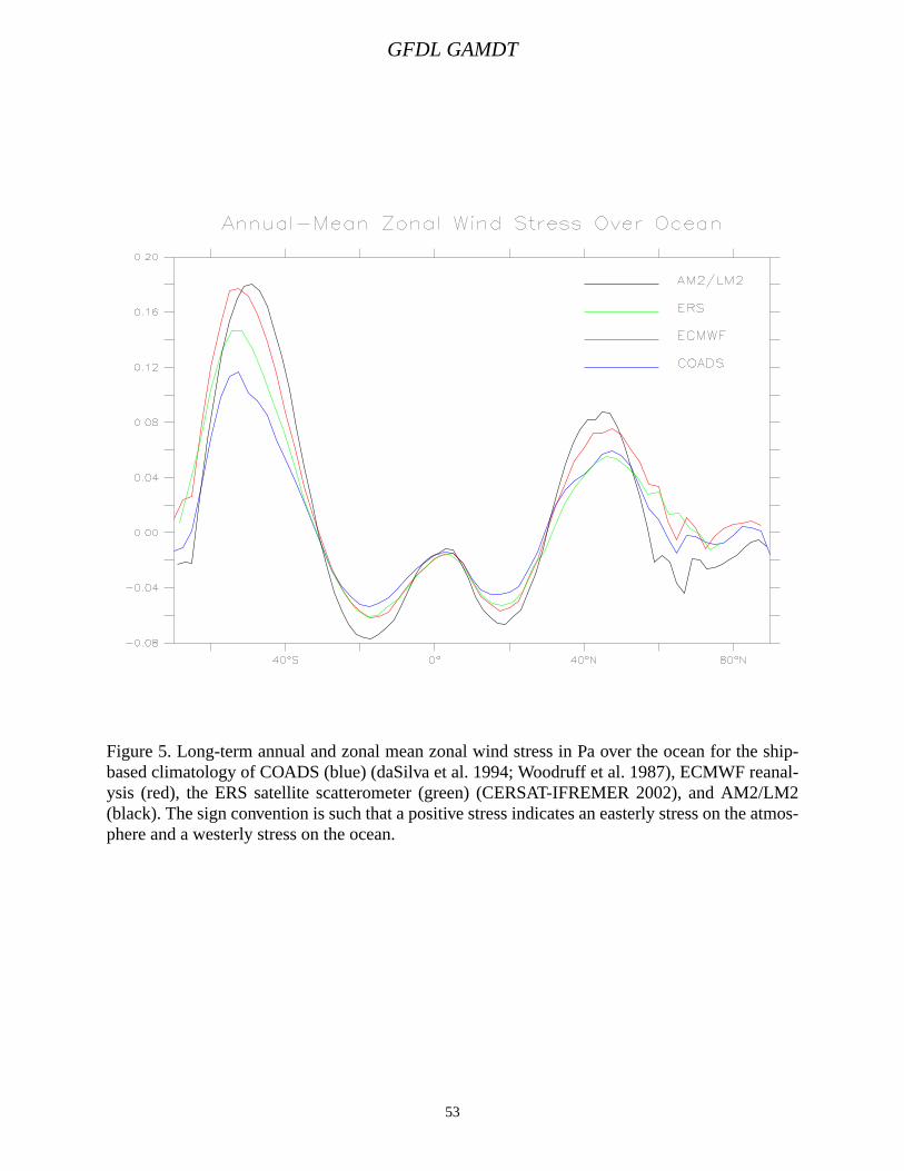
GFDL GAMDT

53

Figure 5. Long-term annual and zonal mean zonal wind stress in Pa over the ocean for the ship-based climatology of COADS (blue) (daSilva et al. 1994; Woodruff et al. 1987), ECMWF reanal-ysis (red), the ERS satellite scatterometer (green) (CERSAT-IFREMER 2002), and AM2/LM2(black). The sign convention is such that a positive stress indicates an easterly stress on the atmos-phere and a westerly stress on the ocean.

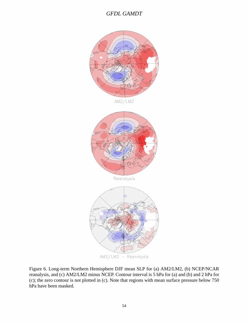
GFDL GAMDT

54

Figure 6. Long-term Northern Hemisphere DJF mean SLP for (a) AM2/LM2, (b) NCEP/NCARreanalysis, and (c) AM2/LM2 minus NCEP. Contour interval is 5 hPa for (a) and (b) and 2 hPa for(c); the zero contour is not plotted in (c). Note that regions with mean surface pressure below 750hPa have been masked.

GFDL GAMDT

55

Figure 7. Long-term DJF mean departure of 500 hPa geopotential height from its zonal mean for(a) AM2/LM2, (b) NCEP/NCAR reanalysis climatology, and (c) AM2/LM2 minus NCEP. Con-tour interval is 25 m in (a) and (b) and 10 m in (c). Statistics at the bottom of (a) and (b) includethe Northern Hemisphere mean and standard deviation. Statistics at the bottom of (c) include thedifference in Northern Hemisphere means, the root mean square error, and the correlation coeffi-cient.

GFDL GAMDT

56

Figure 8. Annual long-term mean precipitation in mm d-1 for (a) AM2/LM2, (b) CMAP observa-tions, and (c) AM2/LM2 minus CMAP. Statistics at the bottom of (a) and (b) include the globalmean and standard deviation. Statistics at the bottom of (c) include the difference in global means,the correlation coefficient, and the root mean square error.

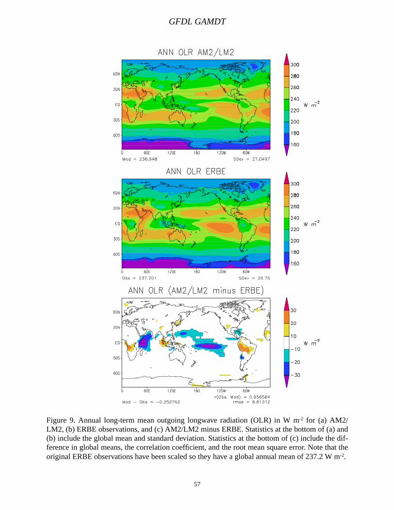
GFDL GAMDT

57

Figure 9. Annual long-term mean outgoing longwave radiation (OLR) in W m-2 for (a) AM2/LM2, (b) ERBE observations, and (c) AM2/LM2 minus ERBE. Statistics at the bottom of (a) and(b) include the global mean and standard deviation. Statistics at the bottom of (c) include the dif-ference in global means, the correlation coefficient, and the root mean square error. Note that theoriginal ERBE observations have been scaled so they have a global annual mean of 237.2 W m-2.

GFDL GAMDT

58

Figure 10. Annual long-term mean absorbed solar radiation (SWAbs) in W m-2 for (a) AM2/LM2,(b) ERBE observations, and (c) AM2/LM2 minus ERBE. Statistics at the bottom of (a) and (b)include the global mean and standard deviation. Statistics at the bottom of (c) include the differ-ence in global means, the correlation coefficient, and the root mean square error. Note that theoriginal ERBE observations have been scaled so they have a global annual mean of 237.2 W m-2.

GFDL GAMDT

59

Figure 11. Annual long-term mean total cloud amount (fraction) for (a) AM2/LM2, (b) ISCCPobservations, and (c) AM2/LM2 minus ISCCP. Statistics at the bottom of (a) and (b) include theglobal mean and standard deviation. Statistics at the bottom of (c) include the difference in globalmeans, the correlation coefficient, and the root mean square error. Regions with snow or ice at thesurface or a surface elevation greater than 1000 m are not shaded in (a) or (b) as the ISCCP satel-lite estimates at these points are deemed unreliable.

GFDL GAMDT

60

Figure 12. Annual long-term mean upper tropospheric humidity in percent for (a) AM2/LM2, (b)TOVS observations, and (c) TOVS minus AM2/LM2. Statistics at the bottom of (a) and (b) indi-cate the global mean. Statistics at the bottom of (c) include the difference in global means, thecorrelation coefficient, and the root mean square error.

GFDL GAMDT

61

Figure 13. Distributions of the regression coefficients of 200 hPa height versus the standardizedNINO3 SST index, as computed using the ensemble mean of the 10-member AMIP-style integra-tions with the AM2/LM2 (upper panels) and NCEP reanalyses (lower panels) for the December-January-February season of the 1951-2000 period. Results for the northern and southern extrat-ropics are shown in the left and right panels, respectively. Contour interval is 5 m. The zero-con-tour is not plotted.

GFDL GAMDT

62

1.0

0.99

0.95

0.9

0.8

0.7

0.6

0.5

0.40.

30.20.

1

0.0

-

-

-

--

--

----

54

55

57

64 65

69

70

72

73

7582

87

8891

97

-0.5 0 0.5 1 1.5 20

0.5

1

1.5

2

Correlation

Figure 14. Taylor diagram depicting the relationships between the observed DJF 200 hPa heightanomalies in the North Pacific / North American sector (20˚-70˚N, 60˚-180˚W) during selectedENSO events and the corresponding ensemble-mean patterns as simulated in the 10-memberAMIP-style runs with the AM2/LM2. Results for individual warm and cold ENSO events are pre-sented using red and blue dots, respectively. The two-digit label for each dot indicates the year ofthe event in question. The spatial correlation coefficient is given by the cosine of the anglebetween the abscissa and the straight line joining the origin and the dot representing the event ofinterest; correlation values are given along the outer solid arc. The ratio between the simulatedand observed spatial variances is given by the distance between the dot and origin; inner and outersolid arcs indicate ratios of 1 and 1.5, respectively. The root mean square (rms) differencebetween the simulated and observed pattern, as normalized by the spatial variance of the observedfield, is given by the distance between the dot and the point with coordinates (1,0) in the diagram;inner and outer dotted arcs indicate normalized rms differences of 0.5 and 1, respectively.

63

Figure 15. Scatterplots of the precipitation anomalies in three monsoon regions [IND - Indian;AUS - northern Australia; SEA - southeast Asia; boundaries of these regions are depicted in Fig-ure 3 of Lau and Nath (2000)] versus the NINO3 SST anomalies. The abscissa in all panels repre-sents the standardized SST anomaly in the NINO3 region. The ordinate axis represents thestandardized precipitation anomaly in IND during the JJA season (left panels), and in SEA (mid-dle panels) and AUS (right panels) during the DJF season. The upper panels are based on AM2/LM2 output for the 1951-2000 period. The lower panels show the observational estimates pro-vided by GPCP for the shorter period of 1979-2000. In each panel, the anomalies of precipitationand NINO3 index for a given year are jointly depicted by a small dot or square. The outstandingwarm and cold ENSO events are highlighted using colored dots and squares, respectively. Thedata for all remaining years are plotted using black dots. The correlation coefficient for the dataentries in each panel is shown in the upper right corner of that panel. Correlation values based onall available years are given in parentheses. Correlation values based on the available warm andcold ENSO events only are given without parentheses.

-3 -2 -1 0 1 2 3-3

-2

-1

0

1

2

3

Pre

cipi

tati

on a

nom

aly

1957

1965

1969

1972

1982

1987

1991

1997

IND

-3 -2 -1 0 1 2 3-3

-2

-1

0

1

2

3

Pre

cipi

tati

on a

nom

aly

IND

-3 -2 -1 0 1 2 3 4Nino3 SST anomaly

-3

-2

-1

0

1

2

3

4

AM2/LM2 Model Ensemble

SEA

-3 -2 -1 0 1 2 3Nino3 SST anomaly

-3

-2

-1

0

1

2

3

GPCP Observations

SEA

-3 -2 -1 0 1 2 3 4-3

-2

-1

0

1

2

3

1954

1955

1964

1970

1973

1975

1988

AUS

-3 -2 -1 0 1 2 3-3

-2

-1

0

1

2

3AUS

-.70 .80 -.70

-.43 .69 .27(-.06) (.58) (-23)

(-.32) (.59) (-.57)

El N

ino

La

Nin

a

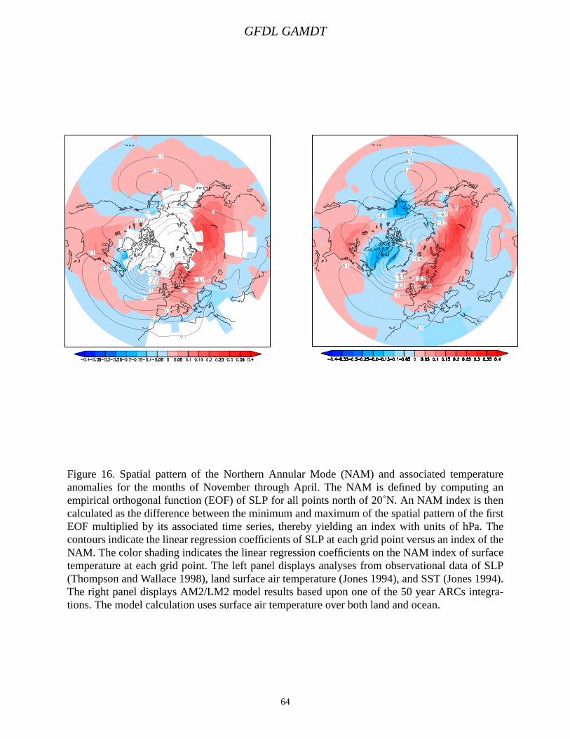
GFDL GAMDT

64

Figure 16. Spatial pattern of the Northern Annular Mode (NAM) and associated temperatureanomalies for the months of November through April. The NAM is defined by computing anempirical orthogonal function (EOF) of SLP for all points north of 20˚N. An NAM index is thencalculated as the difference between the minimum and maximum of the spatial pattern of the firstEOF multiplied by its associated time series, thereby yielding an index with units of hPa. Thecontours indicate the linear regression coefficients of SLP at each grid point versus an index of theNAM. The color shading indicates the linear regression coefficients on the NAM index of surfacetemperature at each grid point. The left panel displays analyses from observational data of SLP(Thompson and Wallace 1998), land surface air temperature (Jones 1994), and SST (Jones 1994).The right panel displays AM2/LM2 model results based upon one of the 50 year ARCs integra-tions. The model calculation uses surface air temperature over both land and ocean.

GFDL GAMDT

65

Figure 17. Frequency of tropical storm genesis for (a) observations and (b) AM2/LM2. Units arenumber of storms per year in a box of size 4˚ latitude by 5˚ longitude.

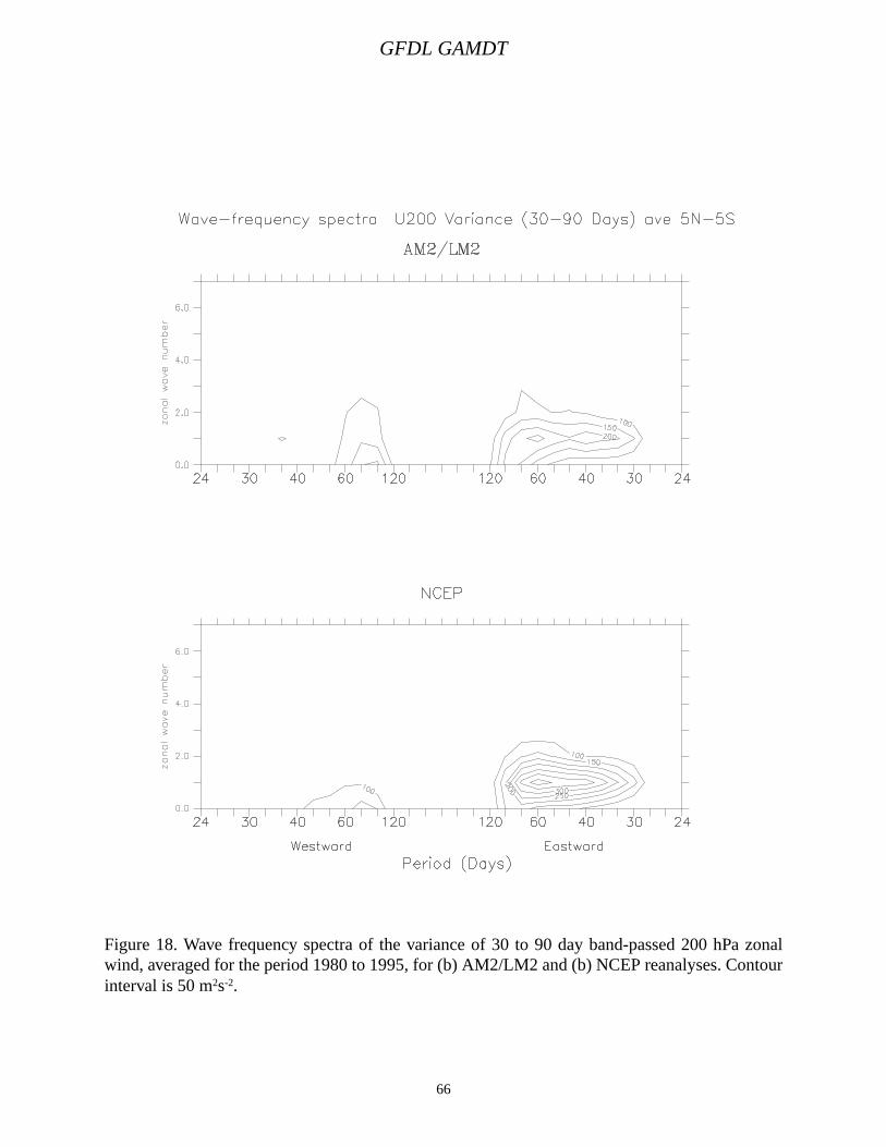
GFDL GAMDT

66

Figure 18. Wave frequency spectra of the variance of 30 to 90 day band-passed 200 hPa zonalwind, averaged for the period 1980 to 1995, for (b) AM2/LM2 and (b) NCEP reanalyses. Contourinterval is 50 m2s-2.

GFDL GAMDT

67

Figure 19. First EOF of 30 to 90 day band-passed precipitation, for the period 1980 to 1995, for(a) AM2/LM2 and (b) CMAP. Units are mm d-1.

GFDL GAMDT

68

-

-

-

-

-

--

-----

1.0

0.99

0.95

0.9

0.8

0.7

0.6

0.5

0.40.

30.20.

1

0.0

0 0.5 .50

0.5

1

1.5

0 0.5 .50

0.5

1

1.5Sea Level Pressure

Correlation

Obs

0.5

1.0

global,ocean only,DJF

-

-

-

-

-

--

-----

1.0

0.99

0.95

0.9

0.8

0.7

0.6

0.5

0.40.

30.20.

1

0.0

0 0.5 .50

0.5

1

1.5

0 0.5 .50

0.5

1

1.5Precipitation

Correlation

Obs

0.5

1.0

30S-30N,ANN

1 1

1 1

-

-

-

-

-

--

-----

1.0

0.99

0.95

0.9

0.8

0.7

0.6

0.5

0.40.

30.20.

1

0.0

0 0.5 1 1.50

0.5

1

1.5

0 0.5 1 1.50

0.5

1

1.5Shortwave Cloud Forcing

Correlation

Obs

0.5

1.0

60S-60N,ANN

Surface Temperature

-

-

-

-

-

--

-----

1.0

0.99

0.95

0.9

0.8

0.7

0.6

0.5

0.40.

30.20.

1

0.0

0 0.5 1 1.50

0.5

1

1.5

0 0.5 1 1.50

0.5

1

1.5

Correlation

Obs

0.5

1.0

30N-90N,land only,JJA

200hPa Z*

-

-

-

-

-

--

-----

1.0

0.99

0.95

0.9

0.8

0.7

0.6

0.5

0.40.

30.20.

1

0.0

0 0.5 1 1.50

0.5

1

1.5

0 0.5 1 1.50

0.5

1

1.5

Correlation

Obs

0.5

1.0

30N-90N,DJF

-

-

-

-

-

--

-----

1.0

0.99

0.95

0.9

0.8

0.7

0.6

0.5

0.40.

30.20.

1

0.0

0 0.5 1 1.50

0.5

1

1.5

0 0.5 1 1.50

0.5

1

1.5Total Cloud Amount

Correlation

Obs

0.5

1.0

60S-60N,ANN

-

-

-

-

-

--

-----

1.0

0.99

0.95

0.9

0.8

0.7

0.6

0.5

0.40.

30.20.

1

0.0

0 0.5 1 1.50

0.5

1

1.5

0 0.5 1 1.50

0.5

1

1.5Zonal Surface Wind Stress

Correlation

Obs

0.5

1.0

60S-60N,ocean only,ANN

MCM

AM2/LM2CCM3.5ECHAM4ECMWFHADAM3-

-

-

-

-

--

-----

1.0

0.99

0.95

0.9

0.8

0.7

0.6

0.5

0.40.

30.20.

1

0.0

0 0.5 1 1.50

0.5

1

1.5

0 0.5 1 1.50

0.5

1

1.5 200hPa Zonal Wind

Correlation

Obs

0.5

1.0

global,DJF

{DERF

Figure 20. Taylor diagrams for selected variables comparing the skill of AM2/LM2 (red circle) inreproducing the observed climatology to that of older GFDL models (MCM and DERF, green andorange circles respectively) and other models participating in AMIP II (CCM3.5, ECHAM4,ECMWF, and HADAM3). Note that all non-GFDL models are plotted with a blue diamond toprevent unique identification. The selected variables include those associated with surface climate(SLP, land surface air temperature, and oceanic wind stress, top row), hydrology and clouds (pre-cipitation, shortwave cloud forcing, and total cloud amount, middle row), and upper troposphericcirculation (200 hPa eddy geopotential and zonal wind, bottom row). The observational sourcesfor these data include the NCEP reanalyses for SLP and 200 hPa eddy geopotential and zonalwind, ECMWF reanalyses for oceanic wind stress, ERBE for cloud radiative forcing, ISCCP fortotal cloud amount, CMAP for precipitation and CRU for land surface air temperature. Beneatheach variable name is an indication of the geographical domain and season used in the calculation.

GFDL GAMDT

69

−90 −60 −30 0 30 60 90Latitude

−2

−1

0

1

2

PW

−2

−1

0

1

2

PW

−2

−1

0

1

2P

W

Trenberth & Caron MacdonaldAM2/LM2

a) Atlantic

b) Indo−Pacific

c) All basins

Figure 21. Poleward oceanic heat transport in petawatts (1015 W) from observational based esti-mates and implied by AM2/LM2 (dark black line). The observed estimates are derived fromatmospheric data (Trenberth and Caron 2001; red lines with dashed lines indicating plus or minusone standard error; based on NCEP-derived products) or oceanic data (MacDonald 1998; theirTable 20; circles with error bars). Results are shown for the a) Atlantic, b) Indo-Pacific, and c)world ocean basins.