The New Fama Puzzle - National Bureau of Economic Research · 2018-02-15 · The New Fama Puzzle...

NBER WORKING PAPER SERIES

THE NEW FAMA PUZZLE

Matthieu BussiereMenzie D. ChinnLaurent FerraraJonas Heipertz

Working Paper 24342http://www.nber.org/papers/w24342

NATIONAL BUREAU OF ECONOMIC RESEARCH1050 Massachusetts Avenue

Cambridge, MA 02138February 2018, Revised December 2019

We would like to thank Agnès Bénassy-Quéré, Yin-Wong Cheung, Alexander Chudik, Jeffrey Frankel, Jim Hamilton, Jean Imbs, Ben Johannsen, Joe Joyce, Steve Kamin, Evgenia Passari, Arnaud Mehl, Lucio Sarno, and conference participants at the Banque de France-Sciences Po. “Workshop on Recent Developments in Exchange Rate Economics,” the “Jean Monnet Workshop on Financial Globalization and its Spillovers,” and seminars at the Banque de France, ECB, Brandeis and the University of Adelaide for useful comments. The views expressed do not necessarily reflect those of the Banque de France, the Eurosystem, or the National Bureau of Economic Research.

At least one co-author has disclosed a financial relationship of potential relevance for this research. Further information is available online at http://www.nber.org/papers/w24342.ack

NBER working papers are circulated for discussion and comment purposes. They have not been peer-reviewed or been subject to the review by the NBER Board of Directors that accompanies official NBER publications.

© 2018 by Matthieu Bussiere, Menzie D. Chinn, Laurent Ferrara, and Jonas Heipertz. All rights reserved. Short sections of text, not to exceed two paragraphs, may be quoted without explicit permission provided that full credit, including © notice, is given to the source.

The New Fama PuzzleMatthieu Bussiere, Menzie D. Chinn, Laurent Ferrara, and Jonas Heipertz NBER Working Paper No. 24342February 2018, Revised December 2019JEL No. F31,F41

ABSTRACT

We re-examine the Fama (1984) puzzle – the finding that ex post depreciation and interest differentials are negatively correlated, contrary to what theory suggests – for eight advanced country exchange rates against the US dollar, over the period up to June 2019. The rejection of the joint hypothesis of uncovered interest parity (UIP) and rational expectations – sometimes called the unbiasedness hypothesis – still occurs, but with much less frequency. Strikingly, in contrast to earlier findings, the Fama regression coefficient is positive and large in the period after the global financial crisis. However, using survey based measures of exchange rate expectations, we find much greater evidence in favor of UIP. Hence, the main story for the switch in Fama coefficients in the wake of the global financial crisis is mostly – but not entirely – a change in how expectations errors and interest differentials co-move. The durability of this phenomenon depends on the persistence in patterns in expectations errors, and the variability of those errors as well as of interest differentials.

Matthieu BussiereBanque de France31 rue Croix des Petits Champs75001 [email protected]

Menzie D. ChinnDepartment of EconomicsUniversity of Wisconsin1180 Observatory DriveMadison, WI 53706and [email protected]

Laurent FerraraBanque de FranceInternational Macroeconomics Division49-1374 Derie-Semsi31 rue Croix des Petits Champs75049 Paris Cedex [email protected]

Jonas HeipertzParis School of Economics48 Boulevard de Jourdan75014 [email protected]

1

1. Introduction

Uncovered interest parity – the proposition that anticipated exchange rate changes should

offset interest rate differentials – is one of the most central concepts in international

finance. At the same time, empirical validation of this concept has proven elusive. In fact,

the failure of the joint hypothesis of uncovered interest rate parity (UIP) and rational

expectations – sometimes termed the unbiasedness hypothesis – is one of the most robust

empirical regularities in the literature. The most commonplace explanations – such as the

existence of an exchange risk premium, which drives a wedge between forward rates and

expected future spot rates – have little empirical verification.1

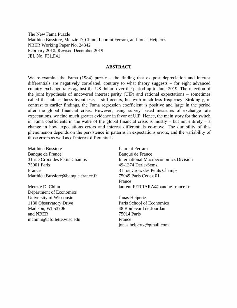
Several developments have prompted this revisit. First and foremost, the last

decade includes a period in which short rates have effectively hit the zero interest rate

bound. This point is clearly illustrated in Figure 1 where we plot one-year interest rates

for a set of eight selected countries and the United States. This development affords us

the opportunity to examine whether the Fama puzzle is a general phenomenon or one that

is regime-dependent. Indeed, the jury is still out about the impact of the zero lower bound

on the relationship between interest rate differentials and exchange rates, for example

Fernald et al. (2017) find no clear evidence that the US dollar has become more sensitive

since 2014. Second, we now have more indicators for risk aversion for extended periods

of time. This potentially allows us to distinguish between competing explanations for the

1 Engel (1996) surveys the failure of the portfolio balance models and consumption capital asset pricing models. See also Chinn (2006) and more recently Engel (2014).

2

failure of the unbiasedness hypothesis. Specifically, we can examine whether the

inclusion of these risk proxies alters the Fama puzzle.2

To anticipate our results, we obtain the following findings. First, Fama’s (1984)

finding that interest rate differentials point in the wrong direction for subsequent ex-post

changes in exchange rates is by and large replicated in regressions for the full sample,

ranging from January 1999 to June 2018. However, the results change if the sample is

truncated to apply to only the most recent decade, the period for which interest rates are

essentially close to zero. For that period, interest differentials correctly signal the right

direction of subsequent exchange rate changes, but with a magnitude that is altogether not

reconcilable with the arbitrage interpretation of UIP. In other words, we obtain positive

coefficients at exactly a time of high risk when it would seem less likely that UIP would

hold.

We also find that the inclusion of a proxy variable for risk, namely the VIX,

results in Fama regression coefficients that are overall similar to those obtained without

accounting for risk aversion. This finding suggests that changes in the elevation of risk as

measured by the VIX do not explain the Fama puzzle, at least not in a direct linear

fashion.

The use of expectations data provides the following insights. First, interest

differentials and anticipated exchange rate changes are overall positively correlated,

consistent with the proposition that investors tend to equalize, at least partially, returns

expressed in common currency terms. Second, in cases where the Fama coefficient

2 The question of exchange rate developments in light of interest rate differentials is obviously important for policy makers in general (and central bankers in particular, see for instance Coeuré, 2017).

3

switches sign from negative to positive from pre- to post-crisis, the result arises because

the correlation of expectations errors and interest differentials changes substantially.

Hence, exchange risk does not appear to be the primary reason why the Fama coefficient

has been so large in recent years (although the altered behaviour of exchange risk does

play a role).

In the next section we briefly lay out the theory underlying the UIP and Fama

regressions, and review the existing literature. In Section 3, we examine the empirical

results obtained from estimating the Fama regression. In Section 4 we explore the results

dropping the rational expectations assumption. Section 5 presents a decomposition of the

components driving the deviation of the Fama coefficient from the posited value of unity.

Section 6 concludes.

2. Theory and Literature

One of the building blocks of international finance, the concept of uncovered interest

parity (UIP) is incorporated into almost all theoretical models. UIP is a no arbitrage

profits condition:

(1) 𝐸𝐸𝑡𝑡𝑀𝑀[𝑠𝑠𝑡𝑡+ℎ − 𝑠𝑠𝑡𝑡] = (𝑖𝑖ℎ,𝑡𝑡 − 𝑖𝑖ℎ,𝑡𝑡∗ )

where 𝑠𝑠𝑡𝑡+ℎ − 𝑠𝑠𝑡𝑡 is the depreciation of the reference currency with respect to the foreign

currency from time 𝑡𝑡 to time 𝑡𝑡 + ℎ, 𝑖𝑖ℎ,𝑡𝑡 and 𝑖𝑖ℎ,𝑡𝑡∗ are the interest rates of horizon ℎ at

time 𝑡𝑡 of the reference and the foreign country, respectively. 𝐸𝐸𝑡𝑡𝑀𝑀 denotes the market’s

expectation based on time 𝑡𝑡 information. To fix ideas and to anticipate on the empirical

results, let 𝑖𝑖ℎ,𝑡𝑡 represent the US interest rate, 𝑖𝑖ℎ,𝑡𝑡∗ the foreign interest rate (that of the UK,

euro area, Japan, etc), and s𝑡𝑡 the number of US dollars per foreign currency unit, such

4

that an increase in s𝑡𝑡 is a depreciation of the dollar. If the US interest rate, for any

maturity h, is above Japan’s interest rate, i.e. 𝑖𝑖𝑡𝑡 > 𝑖𝑖𝑡𝑡∗, then we should expect the dollar to

depreciate at horizon h.

In other words, the market’s expectation of returns is equalized in common

currency terms, so that excess returns are not anticipated ex ante. In practice, the most

common way in which testing the validity of UIP has been implemented is by way of the

Fama regression (Fama, 1984):3

(2) 𝑠𝑠𝑡𝑡+ℎ − 𝑠𝑠𝑡𝑡 = 𝛼𝛼 + 𝛽𝛽�𝑖𝑖ℎ,𝑡𝑡 − 𝑖𝑖ℎ,𝑡𝑡∗ � + 𝑢𝑢𝑡𝑡+ℎ

The OLS regression coefficient β is given by the following expression:

(3) �̂�𝛽 = 𝐶𝐶𝐶𝐶𝐶𝐶(𝑖𝑖ℎ,𝑡𝑡−𝑖𝑖ℎ,𝑡𝑡∗ ,𝑠𝑠𝑡𝑡+ℎ−𝑠𝑠𝑡𝑡)

𝑉𝑉𝑉𝑉𝑉𝑉(𝑖𝑖ℎ,𝑡𝑡−𝑖𝑖ℎ,𝑡𝑡∗ )

Under the joint null hypothesis of uncovered interest parity and rational

expectations, 𝛽𝛽 = 1, and the regression residual is a true random error term, orthogonal

to the interest differential. Note that the intercept 𝛼𝛼 may be non-zero while testing for

UIP using equation (2). A non-zero α may reflect a constant risk premium (hence, tests

for β = 1 are tests for a time-varying risk premium, rather than risk neutrality per se)

and/or approximation errors stemming from Jensen’s Inequality and from the fact that

expectation of a ratio (the exchange rate) is not equal to the ratio of the expectation.

3 For ease of exposition, log approximations are used. In the empirical implementation, exact formulas are used. We have examined data at three month and one year horizons (h ∈ [3,12]), using monthly data. This means the regression residuals are serially correlated under the null hypothesis of rational expectations and uncovered interest parity. We account for this issue by using robust standard errors. We report results for h=12, in order to conserve space; h=3 results are reported in the Appendix Tables 2-4.

5

In order to understand the surprising nature of the results for empirical tests of

uncovered interest parity, it is helpful to clarify what is to be expected from a Fama

regression by isolating the key assumptions necessary to go from equation (1) to

regression equation (2). There are three key assumptions for obtaining (2) from (1), as

laid out in the following equations:

(4) 𝑓𝑓ℎ,𝑡𝑡 − 𝑠𝑠𝑡𝑡 = �𝑖𝑖ℎ,𝑡𝑡 − 𝑖𝑖ℎ,𝑡𝑡∗ � − 𝜖𝜖ℎ,𝑡𝑡

𝑐𝑐𝑖𝑖𝑐𝑐

(5) 𝑓𝑓ℎ,𝑡𝑡 = 𝐸𝐸𝑡𝑡𝑀𝑀[𝑠𝑠𝑡𝑡+ℎ] + 𝜖𝜖ℎ,𝑡𝑡𝑉𝑉𝑐𝑐

(6) 𝑠𝑠𝑡𝑡+ℎ = 𝐸𝐸𝑡𝑡𝑀𝑀[𝑠𝑠𝑡𝑡+ℎ] − 𝜖𝜖𝑡𝑡+ℎ𝑓𝑓

When 𝜖𝜖ℎ,𝑡𝑡𝑐𝑐𝑖𝑖𝑐𝑐 is zero, then equation (4) indicates that there are no barriers to arbitrage using

the forward rate 𝑓𝑓ℎ,𝑡𝑡(of horizon h, at time t). In other words, covered interest parity holds,

or equivalently, the covered interest differential is zero. This condition applies when

capital controls are not relevant, and there are no regulatory or funding constraints.4 For

currency pairs of advanced economies, and for offshore yields,5 covered interest parity

has held up, up until the global financial crisis. Equation (5) indicates that the forward

rate is equal to the market’s expectation of the future spot rate up to an exchange risk

premium term, 𝜖𝜖ℎ,𝑡𝑡𝑉𝑉𝑐𝑐 . This is tautology, unless greater structure is imposed.6

The combination of 𝜖𝜖ℎ,𝑡𝑡𝑐𝑐𝑖𝑖𝑐𝑐 = 𝜖𝜖ℎ,𝑡𝑡

𝑉𝑉𝑐𝑐 = 0 in Equations (4) and (5) yields uncovered

interest rate parity. Only when combined with the assumption of rational expectations, 4 See Dooley and Isard (1980) for discussion and Popper (1993) for a review of the pre-2008 experience, in which the covered interest differential is attributed to political risk. 5 Note that we use offshore yields rather than sovereign bond yields, thereby mitigating the convenience yield channel emphasized by Engel (2016). 6 See Engel (1996) for a discussion of how the forward rate and the expected spot rate might deviate even under rational expectations and risk neutrality.

6

namely 𝐸𝐸𝑡𝑡�𝜖𝜖𝑡𝑡+ℎ𝑓𝑓 � = 0 in equation (6)7, does one obtain the regression equation (2), where

the regression residual can be interpreted as the forecast error. In general, the 𝛽𝛽 = 1

hypothesis can be seen to rely upon several moment conditions:

(7) 𝑝𝑝𝑝𝑝𝑖𝑖𝑝𝑝(�̂�𝛽) = 1 −𝐶𝐶𝐶𝐶𝐶𝐶�𝑖𝑖ℎ,𝑡𝑡−𝑖𝑖ℎ,𝑡𝑡

∗ ,𝜖𝜖ℎ,𝑡𝑡𝑐𝑐𝑐𝑐𝑐𝑐�

𝑉𝑉𝑉𝑉𝑉𝑉�𝑖𝑖ℎ,𝑡𝑡−𝑖𝑖ℎ,𝑡𝑡∗ �

−𝐶𝐶𝐶𝐶𝐶𝐶�𝑖𝑖ℎ,𝑡𝑡−𝑖𝑖ℎ,𝑡𝑡

∗ ,𝜖𝜖ℎ,𝑡𝑡𝑟𝑟𝑐𝑐�



∗ ,𝜖𝜖𝑡𝑡+ℎ𝑓𝑓 �


When the covered interest differential is zero, the first covariance term is zero. This has

been the conventional approach; however, recent work has documented the fact that

covered interest differentials have increased in recent years (Borio et al., 2016; Du et al.,

2018), and so we do not impose this assumption in our analysis. In the absence of covered

interest differentials, as long as there is a time varying risk premium or biased

expectations, then 𝑝𝑝𝑝𝑝𝑖𝑖𝑝𝑝(�̂�𝛽) will deviate from unity.

The literature testing variants of the uncovered interest rate parity hypothesis is

vast and varied. Most of the studies fall into the category employing the rational

expectations hypothesis; in our lexicon, that means they are tests of the unbiasedness

hypothesis. Estimates of equation (6) using horizons for up to one year typically reject

the unbiasedness restriction on the slope parameter. For instance, the survey by Froot and

Thaler (1990), finds an average estimate for β of -0.88.8 Bansal and Dahlquist (2000)

provide more mixed results, when examining a broader set of advanced and emerging

market currencies. They also note that the failure of unbiasedness appears to depend upon

7 Note that the definition of the expectation or forecast error is the negative of the convention, i.e., actual minus forecast. 8 Similar results are cited in surveys by MacDonald and Taylor (1992) and Isard (1995). Meese and Rogoff (1983) show that the forward rate is outpredicted by a random walk, which is consistent with the failure of the unbiasedness hypothesis.

7

whether the US interest rate is above or below the foreign interest rate.9 10 Frankel and

Poonawala (2010) document that for emerging markets more generally, the unbiasedness

hypothesis coefficient is typically more positive.11

The poor performance of the interest differential as a predictor shows up in other

ways. At short horizons, the interest differential is outperformed by a random walk model

of the exchange rate (Cheung et al., 2005; Cheung et al., 2019). However, at longer

horizons, the interest differential does much better than a random walk, mirroring the

fewer rejections of the unbiasedness hypothesis at longer horizons documented by Chinn

and Meredith (2004).

There is an alternative approach that involves using survey-based data to measure

exchange rate expectations. In this case, the error term in equation (6), 𝜖𝜖𝑡𝑡+ℎ𝑓𝑓 , need not be

a true innovation. It could have a non-zero mean, be serially correlated, and perhaps

correlated with the interest differential. Froot and Frankel (1989) were early expositors of

this approach. In a related vein, Chinn and Frankel (1994) document that it was more

difficult to reject UIP for a broad set of currencies when using survey based forecasts.

Similar results were obtained by Chinn and Frankel (2019), when extending the data up

to 2009, increasing the sample to about 32 years. This pattern of findings suggests that

the assumption of rational expectations is not innocuous, and that the examination of the

9 Flood and Rose (1996, 2002) note that including currency crises and devaluations, one finds more evidence for the unbiasedness hypothesis. 10 See Hassan and Mano (2017) for a different perspective on how the Fama puzzle relates to the carry trade. 11 Chinn and Meredith (2004) tested the UIP hypothesis at five year and ten year horizons for the Group of Seven (G7) countries, and found greater support for the UIP hypothesis holding at these long horizons than at shorter horizons of three to twelve months. The estimated coefficient on the interest rate differentials were positive and were closer to the value of unity than to zero in general.

8

UIP condition both assuming and dispensing with the rational expectation assumption is

warranted.

One approach we will not investigate is the bias arising from improper restrictions

in the estimation methodology, such as coefficient restrictions when there is substantial

persistence (Moore, 1994; Zivot, 2000), unbalanced regressions (Maynard and Phillips,

2001), nonlinearity due to thresholds (Baillie and Kilic, 2006), and issues of cointegration

(Chinn and Meredith, 2005).

3. Fama Regressions

We collected monthly data for the interest rates and currencies of eight economies --

Canada, Switzerland, Japan, Denmark, Norway, Sweden, UK and the euro area – over the

Jan. 1999 – June 2019 period. We examined offshore interest rates of twelve month

maturities; the use of offshore interest rates has historically obviated the need to account

for the impact of capital controls.12

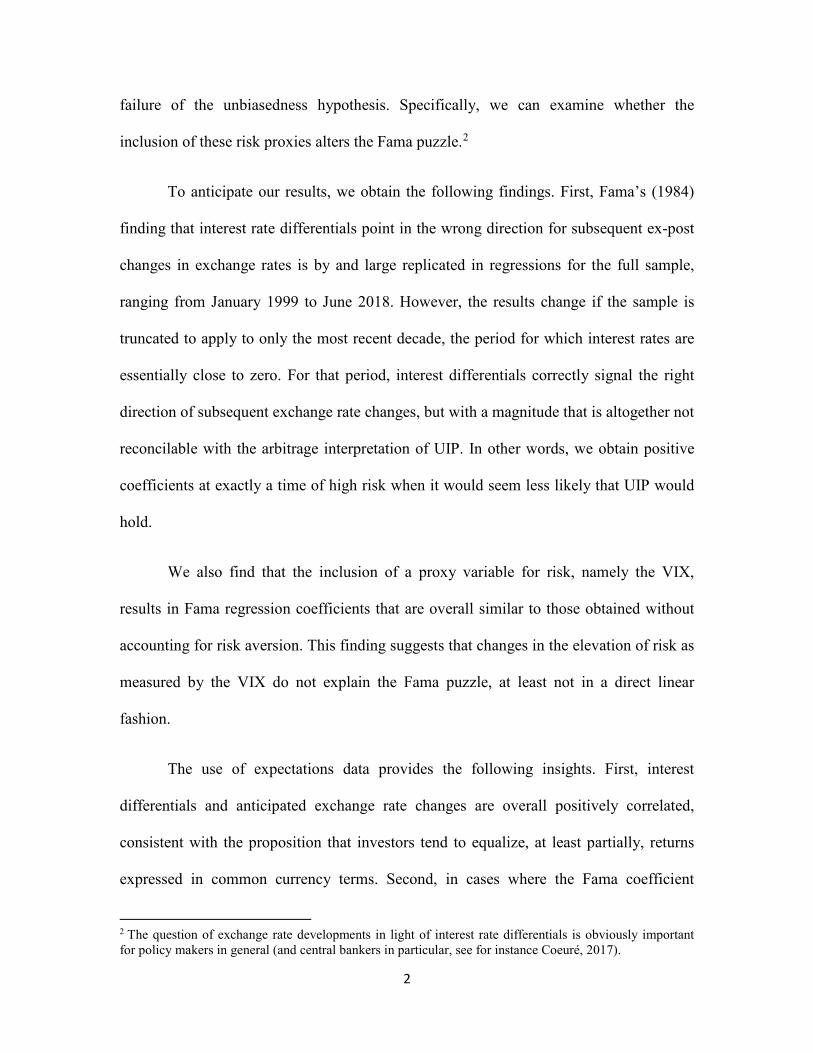
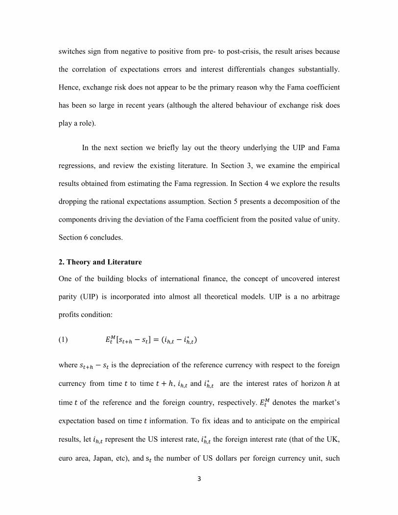
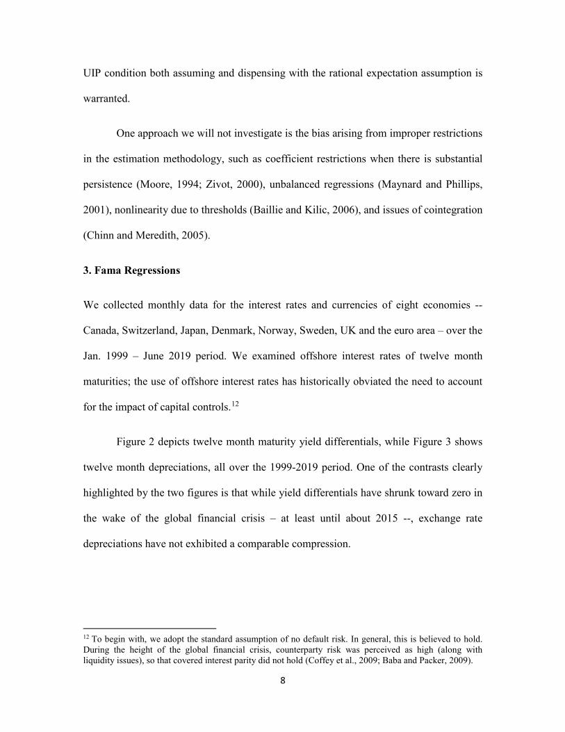
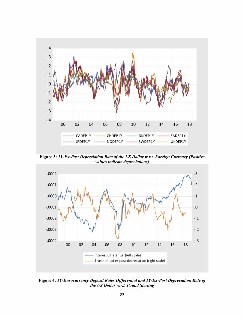
Figure 2 depicts twelve month maturity yield differentials, while Figure 3 shows

twelve month depreciations, all over the 1999-2019 period. One of the contrasts clearly

highlighted by the two figures is that while yield differentials have shrunk toward zero in

the wake of the global financial crisis – at least until about 2015 --, exchange rate

depreciations have not exhibited a comparable compression.

12 To begin with, we adopt the standard assumption of no default risk. In general, this is believed to hold. During the height of the global financial crisis, counterparty risk was perceived as high (along with liquidity issues), so that covered interest parity did not hold (Coffey et al., 2009; Baba and Packer, 2009).

9

Table 1 reports in Panel A the results from equation (2) at the twelve month

horizon, for the full sample.13 The results are largely in accord with previous findings. In

general, the slope coefficients on the interest differential (i.e., the “Fama coefficient”) are

negative, although the coefficients are not statistically different from zero in most cases.

Given that under the maintained hypothesis the coefficient should be unity, we also test if

the coefficients are different from unity. It turns out that only the Swiss Franc differs

significantly from one. Even when the coefficients are not significantly different from

unity, it is important to recall that the proportion of variation explained is very small.

The Fama regression represents a non-structural relationship. There is little reason

to believe the same results will hold over time, in the face of changes in the ways policies

are implemented. For instance, as policy regimes change, the expectation formation

process will change too. Changes in the general economic environment will also have an

impact. The global financial crisis provides an obvious break-point to examine. We

carried out various statistical tests to precisely identify the break date. All the eight

currencies involved in our analysis exhibit a significant break over the sample, but there

is no common date that immediately comes out of the analysis. However, all the

currencies show a significant break around the years 2007-08, according to a Chow test.

In this respect we decide to choose August 2007 (which corresponds to August 2006 for

the one year interest rates) as a common break date, keeping in mind that the summer

2007 can be considered as the beginning of the Global Financial Crisis, with the turmoil

on the US housing market. Indeed, on August 9, 2007, BNP Paribas announced that it

was closing three hedge funds that specialised in US mortgage debt. This event is often

13 Since we are examining one year horizons, the interest rate sample is truncated at 2018M06.

10

considered as one of the first tangible signals of the financial crisis as it was followed by

a freeze on the interbank lending market. According to the NBER Dating Committee, the

US economic recession started three months later in December 2007. Thus separating the

sample into pre- and post-crisis periods with ex post exchange rate depreciations ending

August 2007 as break point (interest rates ending at August 2006), we obtain the results

presented in Panel B and Panel C of Table 1. In the pre-crisis period, the coefficients are

uniformly negative, significantly different from unity.

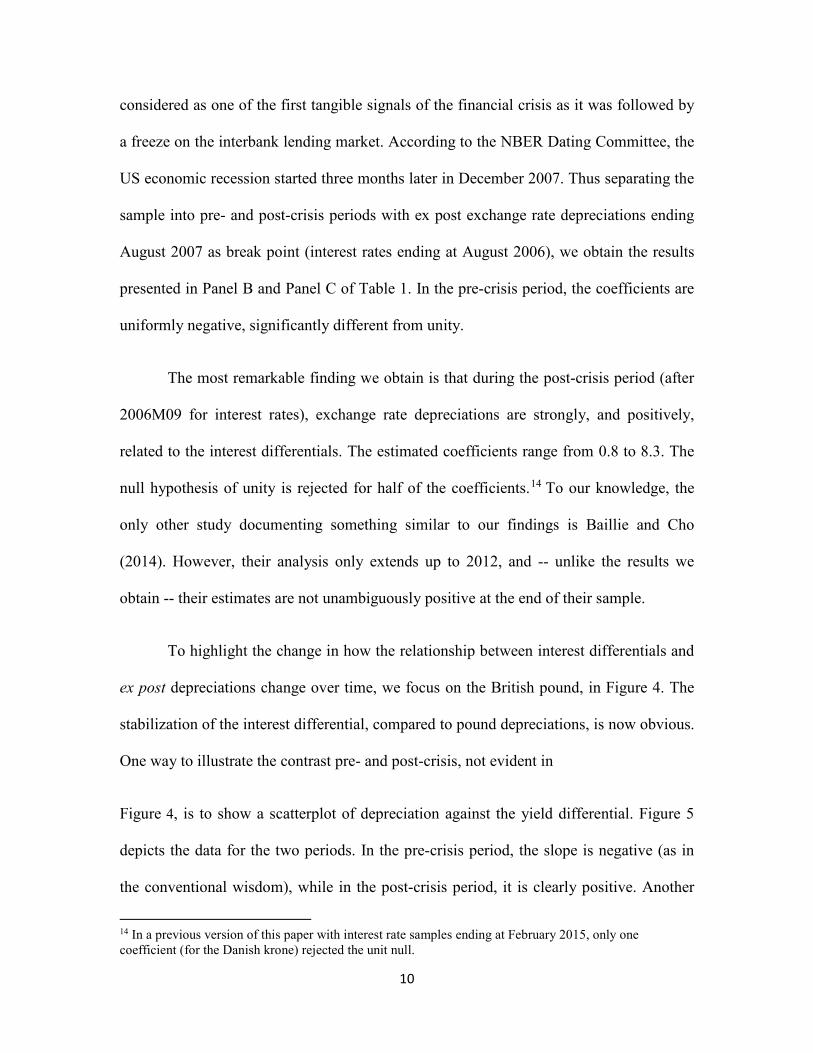
The most remarkable finding we obtain is that during the post-crisis period (after

2006M09 for interest rates), exchange rate depreciations are strongly, and positively,

related to the interest differentials. The estimated coefficients range from 0.8 to 8.3. The

null hypothesis of unity is rejected for half of the coefficients.14 To our knowledge, the

only other study documenting something similar to our findings is Baillie and Cho

(2014). However, their analysis only extends up to 2012, and -- unlike the results we

obtain -- their estimates are not unambiguously positive at the end of their sample.

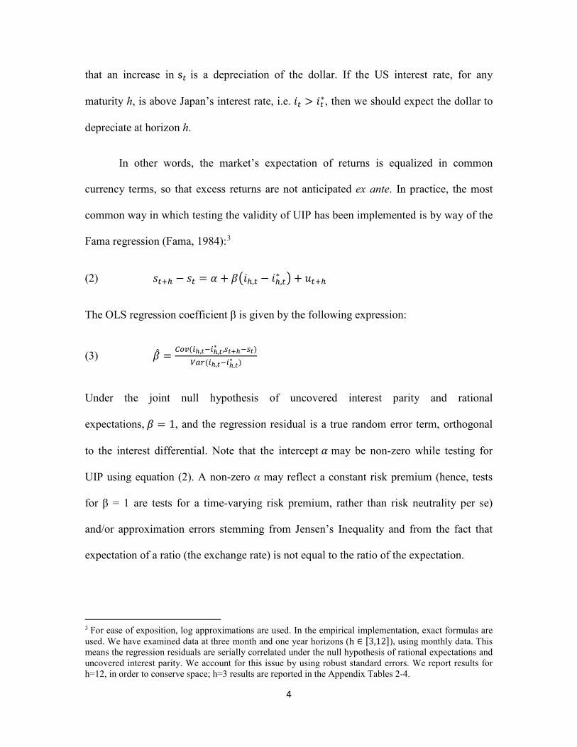
To highlight the change in how the relationship between interest differentials and

ex post depreciations change over time, we focus on the British pound, in Figure 4. The

stabilization of the interest differential, compared to pound depreciations, is now obvious.

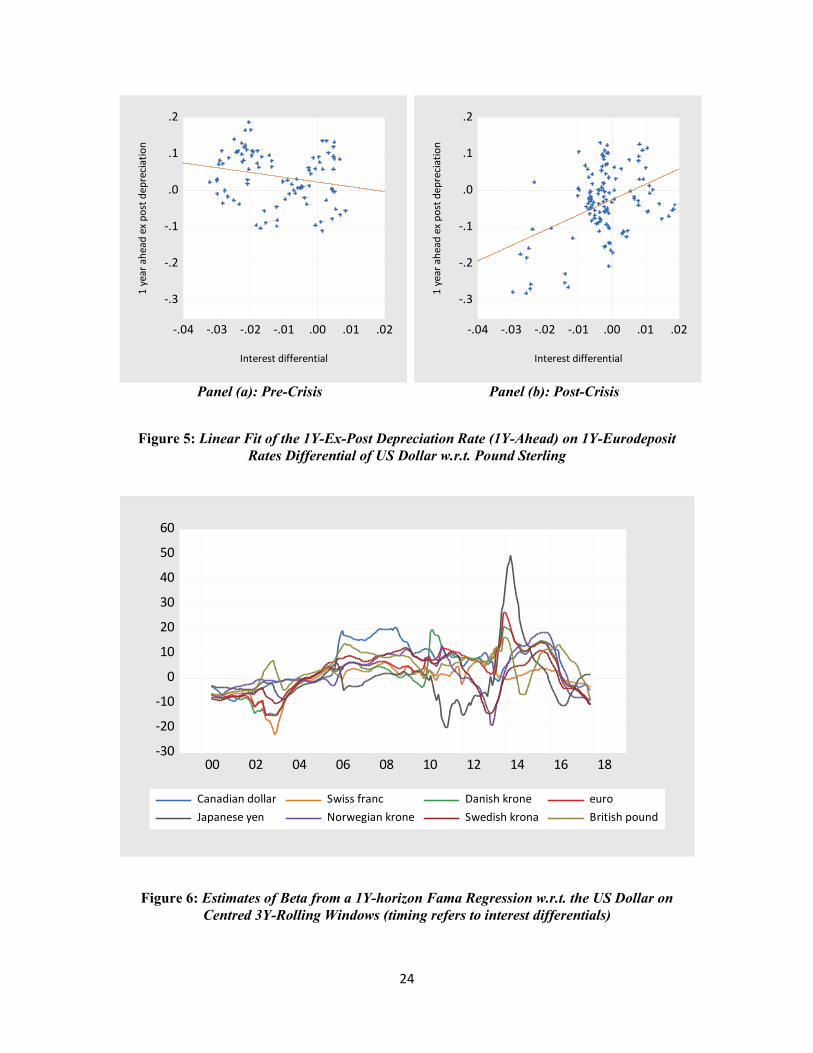
One way to illustrate the contrast pre- and post-crisis, not evident in

Figure 4, is to show a scatterplot of depreciation against the yield differential. Figure 5

depicts the data for the two periods. In the pre-crisis period, the slope is negative (as in

the conventional wisdom), while in the post-crisis period, it is clearly positive. Another

14 In a previous version of this paper with interest rate samples ending at February 2015, only one coefficient (for the Danish krone) rejected the unit null.

11

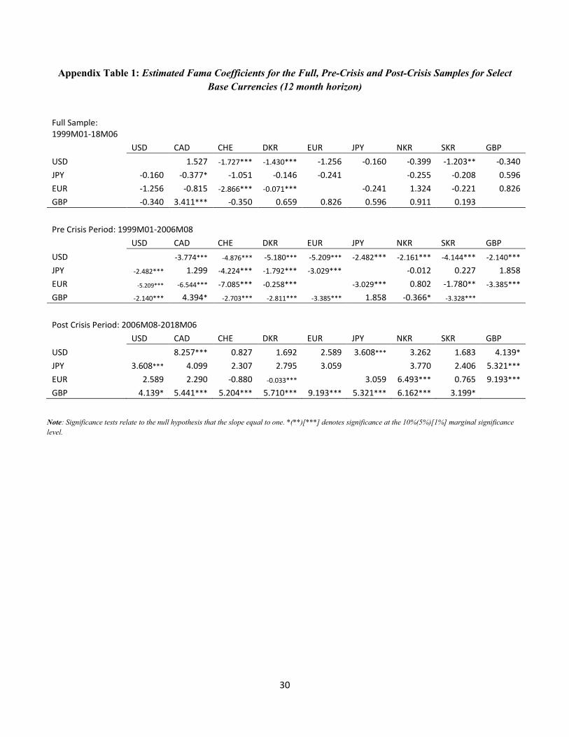
way to illustrate this finding is to show the evolution of the beta coefficients from rolling

Fama regressions. Figure 6 shows beta coefficients obtained from regressing the US

dollar depreciation over twelve months on interest differentials for centred rolling

windows of three years. Results confirm the switch of signs of coefficients from negative

to positive in the post-crisis period. More importantly, most of beta coefficients stay

positive in the aftermath of the global financial crisis (with the exception of the Japanese

yen and the Norwegian krone.), therefore suggesting that a persistent change in

correlations has occurred. Remarkably, this stylized fact holds for various base currencies

(see Appendix Table 1).

These results confront the researcher with at least two questions. The first is the

longstanding puzzle of why the bias exists; the second is why the correlation changed so

much after the crisis.

With respect to the first question, one approach is to allow for an exchange risk

premium, i.e., drop the assumption of 𝜖𝜖𝑡𝑡𝑉𝑉𝑐𝑐 = 0 (but retain the assumption of 𝜖𝜖𝑡𝑡

𝑐𝑐𝑖𝑖𝑐𝑐 = 0).

Doing so means that the error 𝑢𝑢𝑡𝑡+ℎ in 𝑠𝑠𝑡𝑡+ℎ − 𝑠𝑠𝑡𝑡 = 𝛼𝛼 + 𝛽𝛽�𝑖𝑖ℎ,𝑡𝑡 − 𝑖𝑖ℎ,𝑡𝑡∗ � + 𝑢𝑢𝑡𝑡+ℎ includes a

term that is potentially correlated with the interest differential. A potential solution is to

include as an additional regressor some variable that proxies for an exchange risk

premium, 𝜖𝜖𝑡𝑡𝑉𝑉𝑐𝑐. This suggests the following regression equation:15

(8) 𝑠𝑠𝑡𝑡+ℎ − 𝑠𝑠𝑡𝑡 = 𝛼𝛼 + 𝛽𝛽�𝑖𝑖ℎ,𝑡𝑡 − 𝑖𝑖ℎ,𝑡𝑡∗ � + 𝛾𝛾𝑍𝑍𝑡𝑡 + 𝑢𝑢𝑡𝑡+ℎ,

15 If the exchange risk premium is a mean zero random error term, there is no need to include a proxy variable. If, however, there is a central bank reaction function that essentially makes the error term correlated with the interest differential (as in a Taylor rule), then the estimates obtained from a simple Fama regression will be biased. Variants of this approach include McCallum (1994), in which the central bank responds to exchange rate depreciation, and Chinn and Meredith (2004), in which exchange rate depreciation feeds into output and inflation gaps that determine central bank policy rates. See also Mark and Wu (1998) and Engel (2014).

12

where 𝑍𝑍 is a proxy variable.

We evaluate the results using the VIX as a proxy measure 16. The VIX is a

commonly used measure of (inverse) risk appetite, and has been shown to have

substantial explanatory power for exchange rates (Hossfeld and MacDonald, 2015,

Ismailov and Rossi, 2018) and for excess returns (Brunnermeier et al., 2008, Habib and

Stracca, 2012, or Husted et al., forthcoming).17

The results of the VIX augmented Fama regressions are reported in Table 2 and

are notable in the following sense. The inclusion of the VIX does not alter the basic

pattern of results for the Fama coefficient estimates found in Panel A of Table 1.

However, the estimate of the VIX coefficient is typically negative, though only

significant half of the time. This means that when the VIX rises, the dollar appreciates

relative to the foreign currency, even after controlling for the interest rate differential.

Only in the case of the Japanese yen and the Swiss franc, well known safe haven

currencies, does the reverse occur.18

4. Testing UIP with Survey Data

Another way of testing whether arbitragers equalize expected returns is by

dropping the assumption of mean zero expectations error, namely 𝐸𝐸𝑡𝑡�𝜖𝜖𝑡𝑡+1𝑓𝑓 � = 0 in

equation (6). It might be that agents are truly irrational, they use bounded rationality, or

16 Note that we also evaluate inflation differentials (and industrial production growth differentials) as proxies for a premium, in this case a liquidity premium, in line with Engel et al.’s (2019) model of forward rate bias (and high interest-high value currencies). However, we do not obtain empirical evidence for the usefulness of those variables in explaining the Fama puzzle. 17 See Berg and Mark (2018) for discussion of uncertainty and the risk premium. 18 The results are sensitive to the sample period selected. In other results, we have detected a sensitivity of the Fama coefficient to different levels of the VIX, using threshold regression. Hence, while augmenting the Fama regression with the VIX does not alter the estimates of the Fama coefficient, this result does not speak to whether the VIX enters in some nonlinear fashion.

13

have not completely learned the model governing the economy (or, as in Mark and Wu,

1998, some agents are noise traders).

This means we replace equation (6) with:

(9) �̂�𝑠𝑡𝑡+ℎ𝑀𝑀 = 𝐸𝐸𝑡𝑡𝑀𝑀[𝑠𝑠𝑡𝑡+ℎ] − 𝜖𝜖𝑡𝑡+ℎ𝑀𝑀𝑓𝑓

The observed survey based measure of the future spot rate, �̂�𝑠𝑡𝑡+1𝑀𝑀 , equals the market’s

expectation, up to a mean zero random error.19 There is no assumption, then, that the ex-

ante measure will be an unbiased measure of the ex post measure.

This substitution leads to the following regression equation (where we have not

suppressed the exchange risk premium):

(10) �̂�𝑠𝑡𝑡+ℎ𝑀𝑀 − 𝑠𝑠𝑡𝑡 = 𝛼𝛼 + 𝛽𝛽�𝑖𝑖ℎ,𝑡𝑡 − 𝑖𝑖ℎ,𝑡𝑡∗ � + 𝑢𝑢𝑡𝑡+ℎ

In this case, the regression error impounds the forecast error; there is no guarantee that

this forecast error is mean zero, and uncorrelated with the interest differential -- or for

that matter, the risk proxy.

We use as measures of expectations survey data sourced from Consensus

Forecasts from 2003M01 to 2018M06. Notice that survey data availability necessitates a

change in the sample period.20

The results of the regressions are reported in Table 3. One of the defining features

of the results is (1) the point estimates are almost uniformly positive (except for the

19 In other words, we are assuming Classical measurement error, in line with most other analyses. Constant bias would be impounded in the constant. Time varying bias would be much more problematic. 20 An additional complication is that the interest rates and exchange rates do not align precisely in this data set. Interest rates are sampled at end-of-month, while exchange rates forecasts are sampled usually at the second Monday of the month by Consensus Forecasts.

14

Canadian dollar), and (2) coefficients for the Swiss franc and Japanese yen are

significantly greater than one, confirming that those currencies are considered as safe

havens by practitioners. These results are consistent with those obtained in previous

studies using survey data, including Chinn and Frankel (1993) and Chinn and Frankel

(2019)21.

Why are the results so different going from the ex-post to ex-ante measures? The

reason is that the two measures of exchange rate depreciation differ widely and that the

variation in ex-ante measures is substantially smaller than that of ex-post measures. One

way to highlight the difference in volatilities is to note that the scale typically ranges

from -0.12 to +0.22 for ex ante depreciations, while for ex-post depreciations the range is

-0.30 to +0.34.

Table 3 displays the beta coefficients for both horizons in the pre- and post-crisis

periods. Interestingly, the point estimates for twelve month changes do not point to a

switch in coefficients before and after the crisis.

5. Reconciling the Results

Thus far, we have documented the fact that Fama regressions tend to exhibit shifts in the

estimated parameters, while the regressions using survey data are less subject to such

shifts. This is suggestive of the idea that the characteristics of the expectations are critical

in explaining the structural breaks in the Fama regressions.

21 Skeptics of survey based measures argue that reported forecasts are read off of interest differentials. Chinn and Frankel (1993) note the pattern of relationship between expected spot rates and forwards was consistent with the idea that survey respondents use other information in judging future exchange rate movements. In addition, Cheung and Chinn (2001) survey foreign exchange traders, and find that interest differentials are only one of the inputs forecasters use.

15

To see this point explicitly, consider again the decomposition outlined in equation (7):

(7) 𝑝𝑝𝑝𝑝𝑖𝑖𝑝𝑝��̂�𝛽� = 1 −𝐶𝐶𝐶𝐶𝐶𝐶�𝑖𝑖ℎ,𝑡𝑡−𝑖𝑖ℎ,𝑡𝑡

∗ ,𝜖𝜖ℎ,𝑡𝑡𝑐𝑐𝑐𝑐𝑐𝑐�

𝑉𝑉𝑉𝑉𝑉𝑉�𝑖𝑖ℎ,𝑡𝑡−𝑖𝑖ℎ,𝑡𝑡∗ ��

𝐴𝐴


∗ ,𝜖𝜖ℎ,𝑡𝑡𝑟𝑟𝑐𝑐�

𝑉𝑉𝑉𝑉𝑉𝑉�𝑖𝑖ℎ,𝑡𝑡−𝑖𝑖ℎ,𝑡𝑡∗ ��

𝐵𝐵


∗ ,𝜖𝜖𝑡𝑡+ℎ𝑓𝑓 �


��

𝐶𝐶

,

where the relevant interest differential correlations with the covered interest differential,

exchange risk, and expectation errors are labelled A, B, and C, respectively. From this

decomposition, it is clear that an increase in the estimated β coefficients could in

principle be due to a decrease in A, B, or C. The fact that the use of survey expectations

reduces the presence of structural breaks suggests that the C term, involving forecast

errors, is of crucial importance.

In order to examine this conjecture more formally, we examine the regression

coefficients conforming to A, B, and C inverted so as to present a decomposition of

estimated (black squares) from UIP value (horizontal black line), for the pre- and post-

crisis period, respectively. Estimates at the twelve month horizon are presented in Figure

7 for five currencies. For three currencies for which the Fama coefficient switches

strongly from pre- to post-crisis – the euro, the sterling and the Canadian dollar, – the big

change occurs in the expectations component. This is shown in Figure 7 (a), (d) and (e),

respectively. To be concrete, in the pre-crisis period, forecast errors defined as

𝐸𝐸𝑡𝑡𝑀𝑀[𝑠𝑠𝑡𝑡+ℎ] − 𝑠𝑠𝑡𝑡+ℎ are positively correlated with �𝑖𝑖ℎ,𝑡𝑡 − 𝑖𝑖ℎ,𝑡𝑡∗ � (showing up as a negative

component in the decomposition); that correlation is very negative over the last decade

(showing up as above zero in the figures). Since these components are subtracted from

the value of unity, That drives estimated Fama coefficients from negative to positive

values.

16

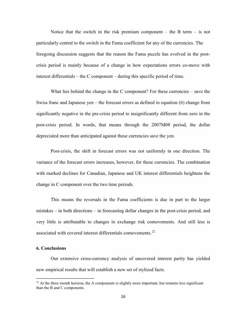
Notice that the switch in the risk premium component – the B term – is not

particularly central to the switch in the Fama coefficient for any of the currencies. The

foregoing discussion suggests that the reason the Fama puzzle has evolved in the post-

crisis period is mainly because of a change in how expectations errors co-move with

interest differentials – the C component – during this specific period of time.

What lies behind the change in the C component? For these currencies – save the

Swiss franc and Japanese yen – the forecast errors as defined in equation (6) change from

significantly negative in the pre-crisis period to insignificantly different from zero in the

post-crisis period. In words, that means through the 2007M08 period, the dollar

depreciated more than anticipated against these currencies save the yen.

Post-crisis, the shift in forecast errors was not uniformly in one direction. The

variance of the forecast errors increases, however, for these currencies. The combination

with marked declines for Canadian, Japanese and UK interest differentials heightens the

change in C component over the two time periods.

This means the reversals in the Fama coefficients is due in part to the larger

mistakes – in both directions – in forecasting dollar changes in the post-crisis period, and

very little is attributable to changes in exchange risk comovements. And still less is

associated with covered interest differentials comovements.22

6. Conclusions

Our extensive cross-currency analysis of uncovered interest parity has yielded

new empirical results that will establish a new set of stylized facts.

22 At the three month horizon, the A components is slightly more important, but remains less significant than the B and C components.

17

First, the bivariate relationship between ex-post depreciation and interest

differentials, as summarized in the Fama regression, is subject to breaks. While such

breaks have shown up in previous studies, the break associated with the global financial

crisis and the subsequent period of low interest rates is quantitatively and qualitatively

much more pronounced. The positive, albeit very large, Fama regression coefficient

detected in the last decade is not usually consistent with uncovered interest parity.

Moreover, even if the coefficient magnitude were consistent with UIP, the finding would

run counter to the intuition that UIP should hold when risk is not important, either

because the environment is not “risky”, or because agents are risk neutral.

Second, we find that the inclusion of a proxy variable for risk, in the form of the

VIX, results in Fama regression coefficients that are largely unchanged. An elevated VIX

typically appreciates the dollar, with few exceptions. Hence, the Fama puzzle is not

explained by risk, at least when proxied by the VIX in a linear specification.

Third, uncovered interest parity regressions estimated using survey data are less

indicative of breaks. That finding suggests that the breakdown in the Fama relationship is

related to the nature of expectations errors.

Fourth, a formal decomposition of deviations from the posited value of unity in

the Fama regression indicates that the switch in signs from pre- to post-crisis can be

attributed to a large extent to the switch in the nature of the co-movement between

expectations errors and interest differentials. This finding implies that the change in the

Fama coefficients is not necessarily a durable one. The phenomenon might dissipate as

the correlation changes, expectations error variability shrinks, or interest rate variability

18

rises – an outcome more likely if a sustained rise of rates above the zero lower bound is

maintained.

19

REFERENCES

Baba, Naohiko, and Frank Packer, 2009, "From turmoil to crisis: dislocations in the FX swap market before and after the failure of Lehman Brothers." Journal of International Money and Finance 28(8): 1350-1374.

Baillie, Richard T. and Dooyeon Cho, 2014, "Time variation in the standard forward premium regression: Some new models and tests." Journal of Empirical Finance 29: 52-63.

Baillie, Richard T., and Rehim Kilic, 2006, "Do asymmetric and nonlinear adjustments explain the forward premium anomaly?" Journal of International Money and Finance 25(1): 22-47.

Bansal, Ravi, and Magnus Dahlquist, 2000, "The forward premium puzzle: different tales from developed and emerging economies." Journal of international Economics 51(1): 115-144.

Berg, Kimberly and Nelson Mark, 2018, “Measures of Global Uncertainty and Carry Trade Excess Returns,” Journal of International Money and Finance 88: 212-227.

Borio, Claudio, Robert Neil McCauley, Patrick McGuire and Vladyslav Sushko, 2016, “Covered interest parity lost: understanding the cross-currency basis,” BIS Quarterly Review, September 2016: 45-64.

Brunnermeier, Markus, Stefan Nagel, and Lasse H. Pedersen, 2008, “Carry Trades and Currency Crashes,” NBER Macroeconomics Annual, 2008 (Feb.)

Cheung, Yin-Wong and Menzie Chinn, 2001, “Currency traders and exchange rate dynamics: a survey of the US market,” Journal of International Money and Finance 20: 439-471.

Cheung, Yin-Wong, Menzie Chinn and Antonio Garcia Pascual, 2005, “Empirical Exchange Rate Models of the Nineties: Are Any Fit to Survive?” Journal of International Money and Finance 24 (November): 1150-1175.

Cheung, Yin-Wong, Menzie Chinn, Antonio Garcia Pascual, and Yi Zhang, 2019, “Exchange Rate Prediction Redux: New Models, New Data, New Currencies,” Journal of International Money and Finance 95: 332-362.

Chinn, Menzie, 2006, “The (Partial) Rehabilitation of Interest Rate Parity: Longer Horizons, Alternative Expectations and Emerging Markets,” Journal of International Money and Finance 25(1) (February): 7-21.

Chinn, Menzie and Jeffrey Frankel, 2019, “A Third of a Century of Currency Expectations Data: The Carry Trade and the Risk Premium,” mimeo (January).

Chinn, Menzie and Jeffrey Frankel, 1994, "Patterns in Exchange Rate Forecasts for 25 Currencies." Journal of Money, Credit and Banking 26(4): 759-770.

Chinn, Menzie and Guy Meredith, 2004, “Monetary Policy and Long Horizon Uncovered Interest Parity.” IMF Staff Papers 51(3): 409-430.

20

Chinn, Menzie and Guy, Meredith, 2005, “Testing Uncovered Interest Parity at Short and Long Horizons during the Post-Bretton Woods Era,” NBER Working Paper No. 11077 (January).

Coffey, Niall, Warren B. Hrung, and Asani Sarkar, 2009, “Capital Constraints, Counterparty Risk, and Deviations from Covered Interest Rate Parity,” Federal Reserve Bank of New York Staff Reports no. 393 (October).

Cœuré, Benoît, 2017, “The international dimension of the ECB’s asset purchase programme,” Speech at the Foreign Exchange Contact Group meeting, 11 July 2017.

Dooley, Michael P., and Peter Isard, 1980, "Capital Controls, Political Risk, and Deviations from Interest-rate Parity." Journal of Political Economy 88(2): 370-384.

Du, Wenxin, Alexander Tepper, Adrien Verdelhan, 2018, “Deviations from Covered Interest Rate Parity,” The Journal of Finance 73(3): 915-957.

Engel, Charles, 1996, “The Forward Discount Anomaly and the Risk Premium: A Survey of Recent Evidence,” Journal of Empirical Finance. 3 (June): 123-92.

Engel, Charles, 2014, “Exchange Rates and Interest Parity.” Handbook of International Economics, vol. 4, pp. 453-522.

Engel, Charles, 2016, “Exchange Rates, Interest Rates, and the Risk Premium,” American Economic Review 106: 436-474.

Engel, Charles, Dohyeun. Lee, Chang Liu, Chenxin Liu and Steve Pak Yeung Wu, 2019, “The uncovered interest parity puzzle, exchange rate forecasting and Taylor rules.” Journal of International Money and Finance 95: 317-331.

Fama, Eugene, 1984, "Forward and Spot Exchange Rates." Journal of Monetary Economics 14: 319-38.

Fernald, J., T. Mertens and P. Shultz, 2017, “Has the dollar become more sensitive to interest rates?”, FRBSF Economic Letter, 2017-18, June 2017.

Flood, Robert P. and Andrew K. Rose, 1996, “Fixes: Of the Forward Discount Puzzle,” Review of Economics and Statistics: 748-752.

Flood, Robert P., and Andrew K. Rose, 2002, "Uncovered interest parity in crisis." IMF Staff Papers 49(2): 252-266.

Frankel, Jeffrey and Menzie Chinn, 1993, "Exchange Rate Expectations and the Risk Premium: Tests for a Cross Section of 17 Currencies." Review of International Economics 1(2): 136-144.

Frankel, Jeffrey, and Jumana Poonawala, 2010, "The forward market in emerging currencies: Less biased than in major currencies." Journal of International Money and Finance 29.3: 585-598.

21

Froot, Kenneth and Jeffrey Frankel, 1989, "Forward Discount Bias: Is It an Exchange Risk Premium?" Quarterly Journal of Economics. 104(1) (February): 139-161.

Froot, Kenneth A., and Richard H. Thaler, 1990, "Anomalies: foreign exchange," The Journal of Economic Perspectives 4(3): 179-192.

Habib, Maurizio M., and Livio Stracca, 2012, "Getting beyond carry trade: What makes a safe haven currency?." Journal of International Economics 87(1): 50-64.

Hassan, Tarek, and Rui Mano, 2017, “Forward and spot exchange rates in a multi-country world.” Mimeo (January).

Hossfeld, Oliver, and Ronald MacDonald, 2015, "Carry funding and safe haven currencies: A threshold regression approach." Journal of International Money and Finance 59: 185-202.

Husted, Lucas, John H. Rogers, and Bo Sun, forthcoming, “Uncertainty, Currency Excess Returns, and Risk Reversals,” Journal of International Money and Finance.

Ismailov, Adilzhan and Barbara Rossi, 2018, “Uncertainty and Deviations from Uncovered Interest Rate Parity,” Journal of International Money and Finance 88: 242-259.

MacDonald, Ronald and Mark P. Taylor, 1992, “Exchange Rate Economics: A Survey,” IMF Staff Papers 39(1): 1-57.

McCallum, Bennett T., 1994, "A reconsideration of the uncovered interest parity relationship." Journal of Monetary Economics 33(1): 105-132.

Mark, Nelson C., and Yangru Wu, 1998, "Rethinking deviations from uncovered interest parity: the role of covariance risk and noise." The Economic Journal 108(451): 1686-1706.

Maynard, Alex, and Peter CB Phillips, 2001, "Rethinking an old empirical puzzle: econometric evidence on the forward discount anomaly." Journal of applied econometrics 16(6): 671-708.

Moore, Michael J., 1994, “Testing for Unbiasedness in Forward Markets,” The Manchester School 62 (Supplement):67-78

Zivot, Eric, 2000, “Cointegration and Forward and Spot Exchange Rate Regressions,” Journal of International Money and Finance 19(6): 785-812.

22

-.01

.00

.01

.02

.03

.04

.05

.06

.07

.08

00 02 04 06 08 10 12 14 16 18

I_1Y_CA/100 I_1Y_CH/100 I_1Y_DK/100 I_1Y_EA/100I_1Y_JP/100 I_1Y_NO/100 I_1Y_SW/100 I_1Y_UK/100I_1Y_US/100

Figure 1: Interest Rates on 1Y-Eurocurrency Deposits

-.06

-.04

-.02

.00

.02

.04

.06

.08

00 02 04 06 08 10 12 14 16 18

CA1YDIF CH1YDIF DK1YDIF EA1YDIFJP1YDIF NO1YDIF SW1YDIF UK1YDIF

Figure 2: 1Y-Eurocurrency Deposit Rates Differential (US Dollar minus Foreign Currency)

23

-.4

-.3

-.2

-.1

.0

.1

.2

.3

.4

00 02 04 06 08 10 12 14 16 18

CADEP1Y CHDEP1Y DKDEP1Y EADEP1YJPDEP1Y NODEP1Y SWDEP1Y UKDEP1Y

Figure 3: 1Y-Ex-Post Depreciation Rate of the US Dollar w.r.t. Foreign Currency (Positive

values indicate depreciations)

-.0004

-.0003

-.0002

-.0001

.0000

.0001

.0002

-.3

-.2

-.1

.0

.1

.2

.3

00 02 04 06 08 10 12 14 16 18

Interest differential (left scale)1 year ahead ex post depreciation (right scale)

Figure 4: 1Y-Eurocurrency Deposit Rates Differential and 1Y-Ex-Post Depreciation Rate of the US Dollar w.r.t. Pound Sterling

24

Panel (a): Pre-Crisis Panel (b): Post-Crisis

Figure 5: Linear Fit of the 1Y-Ex-Post Depreciation Rate (1Y-Ahead) on 1Y-Eurodeposit Rates Differential of US Dollar w.r.t. Pound Sterling

-30

-20

-10

0

10

20

30

40

50

60

00 02 04 06 08 10 12 14 16 18

Canadian dollar Swiss franc Danish krone euroJapanese yen Norwegian krone Swedish krona British pound

Figure 6: Estimates of Beta from a 1Y-horizon Fama Regression w.r.t. the US Dollar on Centred 3Y-Rolling Windows (timing refers to interest differentials)

-.3

-.2

-.1

.0

.1

.2

-.04 -.03 -.02 -.01 .00 .01 .02

Interest differential

1 ye

ar a

head

ex

post

dep

reci

atio

n

-.3

-.2

-.1

.0

.1

.2

-.04 -.03 -.02 -.01 .00 .01 .02

Interest differential

1 ye

ar a

head

ex

post

dep

reci

atio

n

25

(a) Euro

(b) Japanese Yen

(c) Swiss Franc

(d) Pound Sterling

-1

3

-2

1

Pre-crisis Post-crisis

2

-1

3

-3

1

Pre-crisis Post-crisis-5

-1

3

-3

1


2

3

0

1


4

5

26

(e) Canadian Dollar

Inverse Risk Premium (-B) Inverse Covered Interest Dif. (-A) Inverse Expectation Error (-C)

■ Estimate of Beta ▬ Theoretical Beta

Pre-Crisis: 2003M01 – 2006M08 Post-Crisis: 2006M09 – 2018M06

Figure 7: Decomposition of the Deviation from Unity of Estimates of Beta from 1Y-horizon Fama Regressions w.r.t. the US Dollar

1

9

-3

5


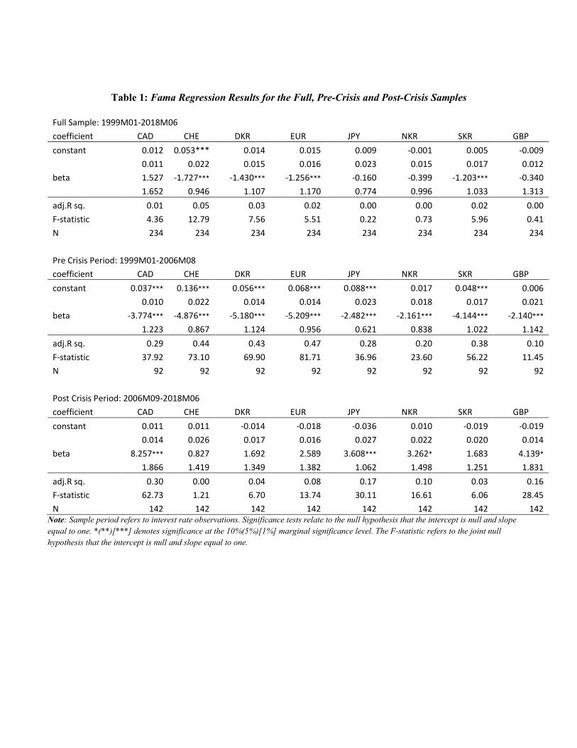
Table 1: Fama Regression Results for the Full, Pre-Crisis and Post-Crisis Samples

Full Sample: 1999M01-2018M06 coefficient CAD CHE DKR EUR JPY NKR SKR GBP

constant 0.012 0.053*** 0.014 0.015 0.009 -0.001 0.005 -0.009

0.011 0.022 0.015 0.016 0.023 0.015 0.017 0.012

beta 1.527 -1.727*** -1.430*** -1.256*** -0.160 -0.399 -1.203*** -0.340 1.652 0.946 1.107 1.170 0.774 0.996 1.033 1.313 adj.R sq. 0.01 0.05 0.03 0.02 0.00 0.00 0.02 0.00 F-statistic 4.36 12.79 7.56 5.51 0.22 0.73 5.96 0.41 N 234 234 234 234 234 234 234 234

Pre Crisis Period: 1999M01-2006M08 coefficient CAD CHE DKR EUR JPY NKR SKR GBP

constant 0.037*** 0.136*** 0.056*** 0.068*** 0.088*** 0.017 0.048*** 0.006

0.010 0.022 0.014 0.014 0.023 0.018 0.017 0.021

beta -3.774*** -4.876*** -5.180*** -5.209*** -2.482*** -2.161*** -4.144*** -2.140*** 1.223 0.867 1.124 0.956 0.621 0.838 1.022 1.142 adj.R sq. 0.29 0.44 0.43 0.47 0.28 0.20 0.38 0.10 F-statistic 37.92 73.10 69.90 81.71 36.96 23.60 56.22 11.45 N 92 92 92 92 92 92 92 92

Post Crisis Period: 2006M09-2018M06 coefficient CAD CHE DKR EUR JPY NKR SKR GBP

constant 0.011 0.011 -0.014 -0.018 -0.036 0.010 -0.019 -0.019

0.014 0.026 0.017 0.016 0.027 0.022 0.020 0.014

beta 8.257*** 0.827 1.692 2.589 3.608*** 3.262* 1.683 4.139* 1.866 1.419 1.349 1.382 1.062 1.498 1.251 1.831 adj.R sq. 0.30 0.00 0.04 0.08 0.17 0.10 0.03 0.16 F-statistic 62.73 1.21 6.70 13.74 30.11 16.61 6.06 28.45 N 142 142 142 142 142 142 142 142

Note: Sample period refers to interest rate observations. Significance tests relate to the null hypothesis that the intercept is null and slope equal to one. *(**)[***] denotes significance at the 10%(5%)[1%] marginal significance level. The F-statistic refers to the joint null hypothesis that the intercept is null and slope equal to one.

28

Table 2: Augmented Fama Regression Results Using the VIX as Proxy for the Risk Premium for the Full Sample (2000M1 – 2018M06)


constant -0.054** 0.015 0.015 0.005 -0.055 -0.063* -0.056 -0.016

0.026 0.031 0.044 0.040 0.035 0.037 0.037 0.024

beta 2.017 -1.444*** -1.436* -1.137* -0.109 0.436 -0.702 -0.280

1.584 0.996 1.323 1.273 0.792 1.234 1.095 1.305

gamma 0.003*** 0.002** 0.000 0.003*** 0.003*** 0.003 0.003 0.000 0.001 0.001 0.002 0.001 0.001 0.002 0.002 0.001 adj.R sq. 0.10 0.06 0.02 0.06 0.06 0.04 0.05 -0.01 F-statistic 14.46 8.99 3.76 7.93 7.93 5.48 7.25 0.30 N 234 234 234 234 234 234 234 234


constant 0.080** 0.160*** 0.128** 0.119* 0.025 0.247*** 0.124* 0.022

0.034 0.061 0.062 0.060 0.046 0.046 0.072 0.055

beta -4.294*** -4.997*** -5.740*** -5.503*** -2.445*** -4.782*** -4.637*** -2.164**

1.216 0.908 1.027 0.923 0.608 0.826 0.911 1.134

gamma -0.002 -0.001 -0.003 0.003 0.003 -0.012*** -0.004 -0.001 0.002 0.002 0.002 0.002 0.002 0.002 0.003 0.002 adj.R sq. 0.32 0.44 0.46 0.33 0.33 0.49 0.40 0.10 F-statistic 22.23 36.79 39.63 23.18 23.18 45.32 31.52 5.89 N 92 92 92 92 92 92 92 92


constant -0.065 -0.065 -0.101 -0.088 -0.123 -0.109 -0.126 -0.063

0.022 0.025 0.046 0.038 0.038 0.030 0.033 0.025

beta 8.357*** 1.855 3.543 3.842 4.049*** 5.347* 2.803 4.993***

1.830 1.365 1.667 1.600 0.952 1.594 1.335 1.885

gamma 0.004*** 0.003*** 0.004** 0.004*** 0.004*** 0.007*** 0.005*** 0.002** 0.001 0.001 0.002 0.001 0.001 0.001 0.001 0.001 adj.R sq. 0.44 0.08 0.12 0.28 0.28 0.32 0.17 0.20 F-statistic 56.00 7.45 10.26 28.01 28.01 33.73 15.90 18.88 N 142 142 142 142 142 142 142 142

Note: Sample period refers to interest rate observations. Significance tests relate to the null hypothesis that the intercept is null, the slope equal to one and the VIX coefficient is null. *(**)[***] denotes significance at the 10%(5%)[1%] marginal significance level. The F-statistic refers to the joint null hypothesis that the intercept is null and slope equal to one.

29

Table 3: UIP Regressions Results Using Survey Data on Exchange Rate Expectations for the Full, Pre-Crisis and Post-Crisis Samples

Full Sample: 2003M01-2018M06

coefficient CAD CHE DKR EUR JPY NKR SKR GBP constant -0.001 -0.055*** -0.017*** -0.018*** -0.061*** 0.030*** 0.020*** -0.003

0.003 0.008 0.005 0.005 0.007 0.004 0.005 0.005

beta 0.245** 2.371*** 1.083 1.272 3.048*** 1.563 1.361 0.770 0.329 0.381 0.317 0.317 0.244 0.266 0.302 0.360 adj.R sq. 0.00 0.35 0.15 0.19 0.61 0.28 0.20 0.07 F-statistic 0.78 107.21 36.58 46.17 306.76 78.87 50.97 15.46 N 198 198 198 198 198 198 198 198


constant -0.003 -0.009 0.011* 0.011 -0.019 0.025*** 0.046*** 0.003

0.005 0.013 0.006 0.006 0.014 0.006 0.007 0.007

beta -0.387*** 1.843* 1.188 1.106 2.355*** 1.161 0.707 0.465* 0.316 0.492 0.373 0.379 0.357 0.250 0.338 0.322 adj.R sq. 0.01 0.33 0.22 0.19 0.61 0.28 0.09 0.05 F-statistic 1.45 22.19 13.27 11.35 67.01 17.87 5.13 3.07 N 44 44 44 44 44 44 44 44


constant -0.001 -0.060*** -0.025*** -0.026*** -0.063*** 0.032*** 0.011** -0.007

0.004 0.007 0.005 0.005 0.008 0.005 0.006 0.005

beta 0.667 1.926*** 0.915 1.169 2.747*** 1.760** 1.460 1.072 0.544 0.355 0.381 0.361 0.338 0.378 0.347 0.535 adj.R sq. 0.01 0.28 0.12 0.17 0.50 0.26 0.21 0.08 F-statistic 2.62 58.64 21.43 31.20 148.35 52.77 40.86 13.14 N 148 148 148 148 148 148 148 148


30

Appendix Table 1: Estimated Fama Coefficients for the Full, Pre-Crisis and Post-Crisis Samples for Select Base Currencies (12 month horizon)

Full Sample: 1999M01-18M06

USD CAD CHE DKR EUR JPY NKR SKR GBP USD

1.527 -1.727*** -1.430*** -1.256 -0.160 -0.399 -1.203** -0.340

JPY -0.160 -0.377* -1.051 -0.146 -0.241

-0.255 -0.208 0.596 EUR -1.256 -0.815 -2.866*** -0.071***

-0.241 1.324 -0.221 0.826

GBP -0.340 3.411*** -0.350 0.659 0.826 0.596 0.911 0.193

Pre Crisis Period: 1999M01-2006M08

USD CAD CHE DKR EUR JPY NKR SKR GBP

USD

-3.774*** -4.876*** -5.180*** -5.209*** -2.482*** -2.161*** -4.144*** -2.140***

JPY -2.482*** 1.299 -4.224*** -1.792*** -3.029***

-0.012 0.227 1.858 EUR -5.209*** -6.544*** -7.085*** -0.258***

-3.029*** 0.802 -1.780** -3.385***

GBP -2.140*** 4.394* -2.703*** -2.811*** -3.385*** 1.858 -0.366* -3.328***

Post Crisis Period: 2006M08-2018M06

USD CAD CHE DKR EUR JPY NKR SKR GBP

USD

8.257*** 0.827 1.692 2.589 3.608*** 3.262 1.683 4.139* JPY 3.608*** 4.099 2.307 2.795 3.059

3.770 2.406 5.321***

EUR 2.589 2.290 -0.880 -0.033***

3.059 6.493*** 0.765 9.193*** GBP 4.139* 5.441*** 5.204*** 5.710*** 9.193*** 5.321*** 6.162*** 3.199*

Note: Significance tests relate to the null hypothesis that the slope equal to one. *(**)[***] denotes significance at the 10%(5%)[1%] marginal significance level.

31

Appendix Table 2: Fama Regression Results for the Full, Pre-Crisis and Post-Crisis Samples

(3 month horizon)


constant 0.012 0.053*** 0.014 0.015 0.009 -0.001 0.005 -0.009

0.011 0.022 0.015 0.016 0.023 0.015 0.017 0.012

beta 1.527 -1.727*** -1.430 -1.256 -0.160 -0.399 -1.203 -0.340 1.652 0.946 1.107 1.170 0.774 0.996 1.033 1.313 adj.R sq. 0.01 0.05 0.03 0.02 0.00 0.00 0.02 0.00 F-statistic 4.36 12.79 7.56 5.51 0.22 0.73 5.96 0.41 N 234 234 234 234 234 234 234 234


constant 0.037*** 0.136*** 0.056*** 0.068*** 0.088*** 0.017 0.048*** 0.006

0.010 0.022 0.014 0.014 0.023 0.018 0.017 0.021

beta -3.774*** -4.876*** -5.180*** -5.209*** -2.482*** -2.161*** -4.144*** -2.140*** 1.223 0.867 1.124 0.956 0.621 0.838 1.022 1.142 adj.R sq. 0.29 0.44 0.43 0.47 0.28 0.20 0.38 0.10 F-statistic 37.92 73.10 69.90 81.71 36.96 23.60 56.22 11.45 N 92 92 92 92 92 92 92 92


constant 0.020 0.026 0.001 -0.002 -0.008 0.039 0.005 -0.002

0.026 0.041 0.029 0.029 0.035 0.029 0.033 0.024

beta 8.060** 0.740 1.883 2.668 2.995 3.766 1.518 5.195 3.649 2.039 2.075 2.265 1.931 2.381 1.884 3.172 adj.R sq. 0.06 -0.01 0.01 0.02 0.03 0.04 0.00 0.06 F-statistic 10.37 0.26 2.49 3.93 5.58 6.93 1.37 10.36 N 148 148 148 148 148 148 148 148


32

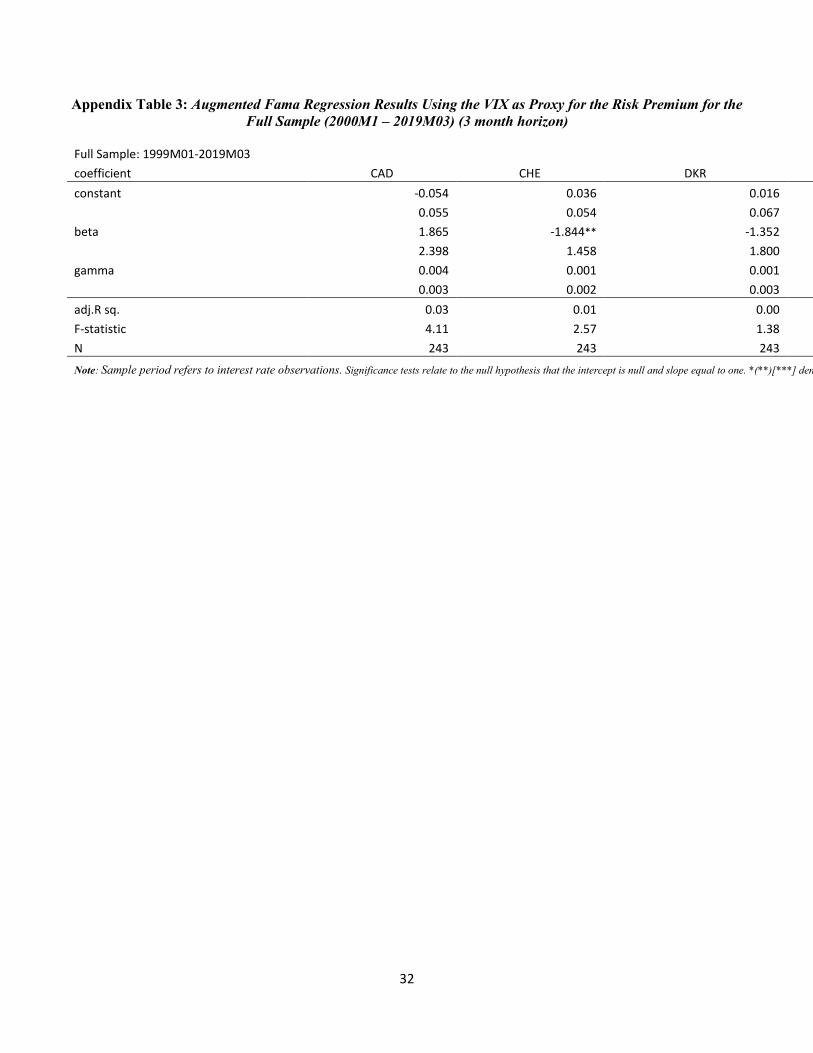
Appendix Table 3: Augmented Fama Regression Results Using the VIX as Proxy for the Risk Premium for the Full Sample (2000M1 – 2019M03) (3 month horizon)

Full Sample: 1999M01-2019M03 coefficient CAD CHE DKR

constant -0.054 0.036 0.016

0.055 0.054 0.067

beta 1.865 -1.844** -1.352

2.398 1.458 1.800

gamma 0.004 0.001 0.001 0.003 0.002 0.003 adj.R sq. 0.03 0.01 0.00 F-statistic 4.11 2.57 1.38 N 243 243 243

Note: Sample period refers to interest rate observations. Significance tests relate to the null hypothesis that the intercept is null and slope equal to one. *(**)[***] den

33

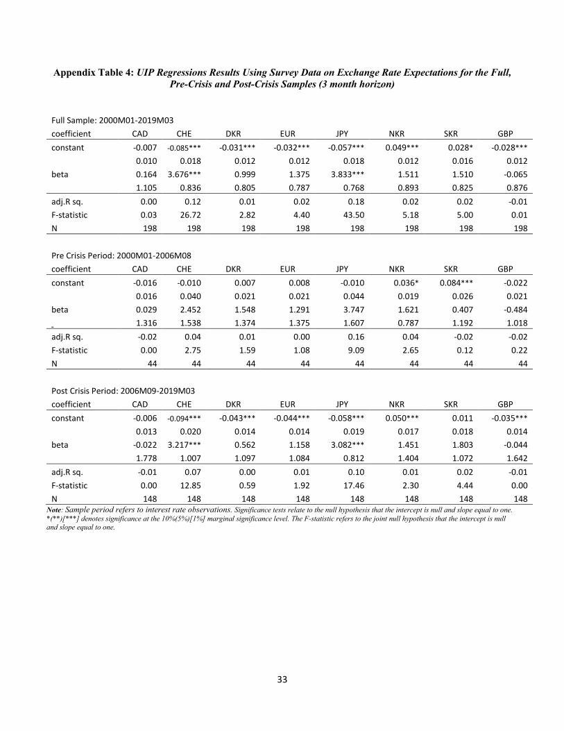
Appendix Table 4: UIP Regressions Results Using Survey Data on Exchange Rate Expectations for the Full, Pre-Crisis and Post-Crisis Samples (3 month horizon)


constant -0.007 -0.085*** -0.031*** -0.032*** -0.057*** 0.049*** 0.028* -0.028***

0.010 0.018 0.012 0.012 0.018 0.012 0.016 0.012

beta 0.164 3.676*** 0.999 1.375 3.833*** 1.511 1.510 -0.065 1.105 0.836 0.805 0.787 0.768 0.893 0.825 0.876 adj.R sq. 0.00 0.12 0.01 0.02 0.18 0.02 0.02 -0.01 F-statistic 0.03 26.72 2.82 4.40 43.50 5.18 5.00 0.01 N 198 198 198 198 198 198 198 198


constant -0.016 -0.010 0.007 0.008 -0.010 0.036* 0.084*** -0.022

0.016 0.040 0.021 0.021 0.044 0.019 0.026 0.021

beta 0.029 2.452 1.548 1.291 3.747 1.621 0.407 -0.484 1.316 1.538 1.374 1.375 1.607 0.787 1.192 1.018 adj.R sq. -0.02 0.04 0.01 0.00 0.16 0.04 -0.02 -0.02 F-statistic 0.00 2.75 1.59 1.08 9.09 2.65 0.12 0.22 N 44 44 44 44 44 44 44 44


constant -0.006 -0.094*** -0.043*** -0.044*** -0.058*** 0.050*** 0.011 -0.035***

0.013 0.020 0.014 0.014 0.019 0.017 0.018 0.014

beta -0.022 3.217*** 0.562 1.158 3.082*** 1.451 1.803 -0.044 1.778 1.007 1.097 1.084 0.812 1.404 1.072 1.642 adj.R sq. -0.01 0.07 0.00 0.01 0.10 0.01 0.02 -0.01 F-statistic 0.00 12.85 0.59 1.92 17.46 2.30 4.44 0.00 N 148 148 148 148 148 148 148 148


34

Appendix Table 5: Data Sources

Variable Source Timing Spot Exchange Rates, against U.S. Dollar

IMF, International Financial Statistics Monthly, End-of-Period, Start: 1999M1

Forward Exchange Rates (3M and 12M), against U.S. Dollar

Thomson Reuters Datastream Daily, End-of-Period, Start: 29/01/1999

Expected Exchange Rates (3M and 12M), against U.S. Dollar

Consensus Forecast Economics Inc.

Monthly, sampled at the second Monday of the month, Start: 2003M1

Eurocurrency Deposit Rates (3M and 12M)

Thomson Reuters Datastream Daily, End-of-Period, Start: 29/01/1999

Volatility S&P 500 Index (VIX) CBOE Daily, End-of-Period, Start: 29/01/1999 Note: If applicable, series are obtained for the following currencies: Canadian Dollar, Danish Krone, Euro, Japanese Yen, Norwegian Krone, Pound Sterling, Swedish Krona, Swiss Franc, United States Dollar

The New Fama Puzzle - National Bureau of Economic Research · 2018-02-15 · The New Fama Puzzle...

Documents

Transcript of The New Fama Puzzle - National Bureau of Economic Research · 2018-02-15 · The New Fama Puzzle...