The neurodynamics of choice, value-based decisions, and preference...

Chapter 13

The neurodynamics of choice,value-based decisions, andpreference reversal

Marius UsherSchool of Psychology, Birkbeck, University of London, London, UK

Anat ElhalalSchool of Psychology, Birkbeck, University of London, London, UK

James L. McClellandDepartment of Psychology, Stanford University, Palo Alto, CA, USA

A theory of choice is paramount in all the domains of cognition requiring behav-ioural output, from perceptual choice in simple psychophysical tasks to motiva-tional value-based choice, often labelled as preferential choice and which is exhibitedin daily decision-making. Until recently, these two classes of choice have been the subject of intensive but separate investigations, within different disciplines.Perceptual choice has been investigated mainly within the experimental psychologyand neuroscience disciplines, using rigorous psychophysical methods that examinebehavioural accuracy, response latencies (choice-RT), and neurophysiological data(Laming, 1968; Ratcliff & Smith, 2003; Usher & McClelland, 2001; Vickers, 1979).Preferential choice, such as when one has to choose an automobile among a set ofalternatives that differ in terms of several attributes or dimensions (e.g., quality andeconomy) has been investigated mainly within the economics and the social sciencedisciplines, using mainly reports of choice preference. Unlike in perceptual choice,where the dominant models are process models that approximate optimality (Bogaczet al., 2007; Gold & Shadlen, 2002) based on the Sequential Probability Ratio Test(SPRT; Barnard, 1946; Wald, 1947), the literature on preferential choice has empha-sised a series of major deviations from normativity (Huber et al., 1982; Kahneman &Tversky, 1979, 2000; Knetch, 1989; Simonson, 1989; Tversky, 1972; Tversky &Kahneman, 1991). This has led to the proposal that decision-makers use a set of disparate heuristics, each addressing some other aspect of these deviations

13-Charter&Oaksford-Chap13 3/5/08 11:26 AM Page 277

(LeBoef & Shafir, 2005).1 Because of this, it is difficult to compare the two types oftheories and to discuss their implications for issues related to optimality and to prin-ciples of rational choice.

Two recent types of research are providing, however, the opportunity to bridge thisgap. First, neurophysiological studies of value-based decisions have been carried outon behaving animals (Glimcher, 2004; Sugrue et al., 2004, 2005). Second, a series ofneurocomputational models of preferential choice have been developed, whichaddress the process by which preferential choice is issued (Steward, this volume; Roe et al., 2001; Usher & Mclelland, 2004). It is the synthesis of these two lines of workthat defines the new field of neuroeconomics, whose central aim is to understand theprinciples that underlie value-based decisions and the neural mechanisms throughwhich these principles are expressed in behaviour. A major insight of neuroeconomicsis that these principles can be modelled as implementing an optimising solution tosome survival/reproductive challenge in the evolutionary environment (Wikipedia).

The aim of this chapter is to review some of the neurocomputational work by con-trasting the various processing assumptions and the way they account for one of themost intriguing patterns in the choice data: contextual preference-reversal. We startwith introducing a very simple process model of choice, called the leaky competingaccumulator (LCA) model (Usher & McClelland, 2001), which has been developed toaccount for both perceptual and preferential choice data. We will then review some ofthe data on preference reversal, and on framing effects, which are the main targets of the neurocomputational theories discussed later. Then we will discuss two such theories, the decision-field theory (DFT) developed by Busemeyer and colleagues(Busemeyer & Diederich, 2002, Busemeyer & Johnson, 2003; Diederich, 1997; Roe et al., 2001) and an extension of the LCA. We examine some similarities and contrastsbetween the models that lead to a set of experimental predictions. Finally, we presentexperimental data aimed at testing these predictions and consider their implicationsfor the issue of rationality in choice.

Perceptual-choice, optimality, and the LCA modelConsider a simple task that illustrates a typical example of perceptual choice. In thistask, the observers (humans or animals) are presented with a cloud of moving dots ona computer screen (Britten et al., 1993). On each trial, a proportion of the dots aremoving coherently in one direction, while the remaining dots are moving randomly.The observer’s task is to indicate the direction of prevalent motion. The time of theresponse is either ‘up to the observer’ (and is measured as a function of the stimulusproperty and the response accuracy) or is controlled by a response signal (and theaccuracy is measured as a function of the observation time). This task presents thebasic demand the observer has to accomplish for performing the task: decide which of

THE NEURODYNAMICS OF CHOICE, VALUE-BASED DECISIONS, AND PREFERENCE REVERSAL278

1 One notable exception is work by Tversky and colleagues (e.g., Tversky, 1972; Tversky &Simonson, 1993), who developed a number of mathematically rigorous process models.

13-Charter&Oaksford-Chap13 3/5/08 11:26 AM 78

PERCEPTUAL-CHOICE, OPTIMALITY, AND THE LCA MODEL 279

a number of options match best a noisy signal. As the noise varies in time, a good wayto perform the task is to integrate the evidence from sensory neurons over time (thisis consistent with the neural data; Schall, 2001; Shadlen & Newsome, 2001). This inte-gration averages out the noise, allowing the accuracy of the choice to increase withtime. The quality of the decision (measured in terms of accuracy per time-taken tomake the response, or response-rate) depends on the response-rule and the way inwhich the evidence is integrated.

A variety of models have been proposed to account for rich data patterns thatinvolve not only accuracy and mean-RTs but also RT-distributions (Smith & Ratcliff2004). Here we will focus on one such model, the LCA (Usher & McClelland, 2001),which is framed at a neural level and yet is simple enough so that it can be mathemat-ically analysed and its parameters can be manipulated so as to optimise performance.As the main aim of this chapter is to understand value-based decisions, we will onlypresent a brief summary here, but see Bogacz et al. (2007) for a detailed and rigorousaccount.

The model assumes that for each choice option there is a response unit that accu-mulates evidence in favour of this option. Figure 13.1 illustrates the model, for thecase of binary choice. The accumulation of the evidence (or activation) is subject totemporal decay (or leak) and the various response units compete via lateral (andmutual) inhibition. The decay and the lateral inhibition (k and w) are the importantparameters that affect the network’s choice pattern and performance. In addition eachunit’s activation is truncated at zero, reflecting the biological constraint that activa-tions correspond to neuronal firing rates, which cannot be negative. This is alsoreflected in the use of the threshold-linear output function, f(x). Mathematically thiscan be formulated and simulated as:

dy ky w f y I dt c dWi i jjj i

N

i i= − − ( ) +⎛

⎝

⎜⎜⎜

⎞

⎠

⎟⎟⎟

+=≠

∑1

ii

I1±c I2±c

y1 y2...

Fig. 13.1. LCA model for binary choice. The variables y1 and y2 accumulate noisy evidence (I1, I2). The units compete due to lateral inhibition (w). To generalize for n-choice, one adds units, which compete with each other by lateral (all to all) inhibition (Usher & McClelland, 2001).


where the final term (dW) corresponds to the differential of a (stochastic) Wienerprocess (Gaussian noise of amplitude c). Finally, the response is issued when the firstof the accumulators reaches a common response criterion. This criterion is assumedto be under the control of the observer, reflecting speed-accuracy tradeoffs.

The model’s choice pattern depends essentially on the relative values of the decayand the inhibition parameters. When decay exceeds inhibition the model exhibitsrecency (it favours information that arrives late in time), but when inhibition exceedsdecay, it exhibits primacy. Neither of these results produces the highest accuracy pos-sible. However, when decay and inhibition are balanced (decay = inhibition) the net-work performs optimally. Indeed, in this case the model’s behaviour mimics theoptimal Sequential Probability Ratio Test (SPRT). This means that among all possibleprocedures for solving this choice problem, it minimizes the average decision time(DT) for a given error rate (ER).

One advantage of this neural model over other (more abstract) models such as therandom-walk, is that it is easy to generalise to choice among more than two alterna-tives. In this case, all the units representing the alternative choices race towards a com-mon response criterion, while they all simultaneously inhibit each other. This mutualinhibition allows the network choice to depend on relative evidence, without the needfor a complex readout mechanism that would depend on computing the differencebetween the activations of the most active unit and the next most active. Moreover, asdiscussed in detail in Bogacz et al. (2007), the threshold-nonlinearity (the truncationof negative activations at zero) is critical in maintaining this advantage when theinput favours only a small subset of a larger ensemble of options. The reason for thisis that with the threshold-nonlinearity, the activation of all the non-relevant units ismaintained at zero, rather than becoming negative and sending uninformative (posi-tive) input into the relevant competing units (see Bogacz et al., 2007). This feature isimportant in our application of the LCA model to value-based choice.

Value-based decisions, preference-reversal, and reference effectsAlthough we assume that both perceptual and value/motivational decisions involve acommon selection mechanism, the basis on which this selection operates differs. Theaim of this section is to review the underlying principles of value-based decisions,focusing on a series of puzzling patterns of preference reversal in multi-attributechoice (see Stewart & Simpson, this volume, for a discussion of risky choice), whichraise challenges for an optimal or normative theory of choice.

Unlike in perceptual choice, the preferential choice cannot be settled on the basis ofperceptual information alone. Rather, each alternative needs to be evaluated in rela-tion to its potential consequences and its match to internal motivations. Often, this isa complex process, where the preferences for the various alternatives are being con-structed as part of the decision process itself (Slovic, 1995). In some situations, where theconsequences are obvious or explicitly described, the process can be simplified. Consider,for example, a choice between three flats, which vary on their properties as describedon a number of dimensions (number of rooms, price, distance from work, etc).



VALUE-BASED DECISIONS, PREFERENCE-REVERSAL, AND REFERENCE EFFECTS 281

The immediate challenge facing a choice in such situations is the need to convertbetween the different currencies, associated with the various dimensions. The conceptof value is central to preferential choice, as a way to provide such a universal internalcurrency. Assuming the existence of a value function, associated with each dimension,a simple normative rule of decision-making, the expected-additive-value, seems toresult. Accordingly, one should add the values that an alternative has on each dimen-sion and compute expectation values when the consequences of the alternatives areprobabilistic. Such a rule is then bound to generate a fixed and stable preference orderfor the various alternatives. Behavioural research in decision-making indicates, how-ever, that humans and animals violate expected-value prescriptions and change theirpreferences between a set of options depending on the way the options are describedand on a set of contextual factors.

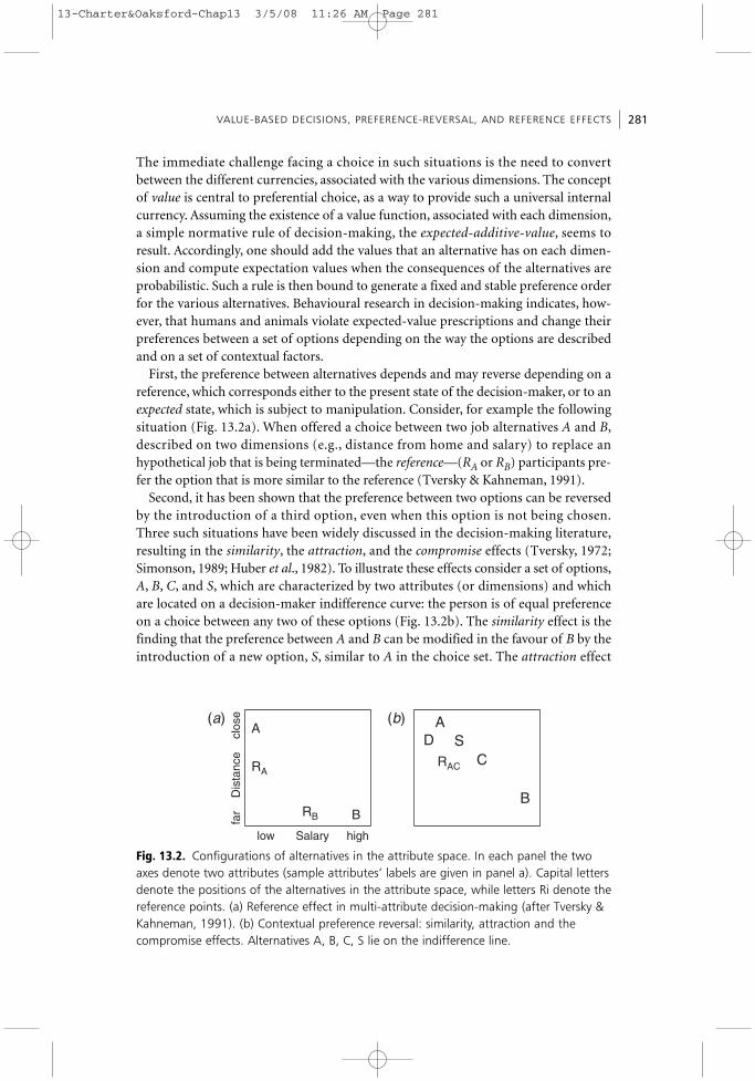
First, the preference between alternatives depends and may reverse depending on areference, which corresponds either to the present state of the decision-maker, or to anexpected state, which is subject to manipulation. Consider, for example the followingsituation (Fig. 13.2a). When offered a choice between two job alternatives A and B,described on two dimensions (e.g., distance from home and salary) to replace anhypothetical job that is being terminated—the reference—(RA or RB) participants pre-fer the option that is more similar to the reference (Tversky & Kahneman, 1991).

Second, it has been shown that the preference between two options can be reversedby the introduction of a third option, even when this option is not being chosen.Three such situations have been widely discussed in the decision-making literature,resulting in the similarity, the attraction, and the compromise effects (Tversky, 1972;Simonson, 1989; Huber et al., 1982). To illustrate these effects consider a set of options,A, B, C, and S, which are characterized by two attributes (or dimensions) and whichare located on a decision-maker indifference curve: the person is of equal preferenceon a choice between any two of these options (Fig. 13.2b). The similarity effect is thefinding that the preference between A and B can be modified in the favour of B by theintroduction of a new option, S, similar to A in the choice set. The attraction effect

BRB

B

DC

far

D

ista

nce

cl

ose(a) (b)

A

RA

SA

RAC

low Salary high

Fig. 13.2. Configurations of alternatives in the attribute space. In each panel the twoaxes denote two attributes (sample attributes’ labels are given in panel a). Capital lettersdenote the positions of the alternatives in the attribute space, while letters Ri denote thereference points. (a) Reference effect in multi-attribute decision-making (after Tversky &Kahneman, 1991). (b) Contextual preference reversal: similarity, attraction and the compromise effects. Alternatives A, B, C, S lie on the indifference line.


corresponds to the finding that, when a new option similar to A, D, and dominated byit (D is worse than A on both dimensions) is introduced into the choice set, the choicepreference is modified in favour of A (the similar option; note that while the similarityeffects favours the dissimilar option, the attraction effect favours the similar one).Finally, the compromise effect corresponds to the finding that, when a new optionsuch as B is introduced into the choice set of two options A and C, the choice is nowbiased in favour of the intermediate one, C, the compromise.

Third, a large number of studies indicate that human (and animal) observersexhibit loss-aversion. A typical illustration of loss-aversion was shown in the followingstudy (Knetch, 1989). Three groups of participants are offered a choice between twoobjects of roughly equal value (a mug and a chocolate bar), labelled here as A and B.One group is first offered the A-object and then the option to exchange it for the B-object. The second group is offered the B-object followed by the option to exchangeit for A. The control group is simply offered a choice between the two objects. Theresults reported by Knetch (1989) are striking. Whereas the control participantschose the two objects in roughly equal fractions (56% vs. 44%), 90% of the partici-pants in either of the groups that were first offered one of the objects prefer to keep itrather than exchange it for the other one (see also Samuelson & Zeckhauser, 1988).This effect is directly explained by Tversky and Kahneman by appealing to an asym-metric value-function, which is steeper in the domains of losses than in that of gains.Because losses are weighted more than gains, participants who evaluate their choiceswith the already-owned object serving as the reference point decline the exchange.[For the control participants the values may be computed either relative to the neutralreference (Tversky & Kahneman, 1991), or each option can be used as a reference forthe other options (Tversky & Simonson, 1993); in both cases, there is no referencebias, consistent with the nearly equal choice fractions in this case.]

Computational models of preferential choice and of reversal effectsRecent work on neurocomputational models on preferential choice (Busemeyer &Diederich, 2002; Busemeyer & Johnson, 2003; Roe et al., 2001; Stewart & Simpson,this volume; Usher & McClelland, 2004) may seem at odds with the emphasis onheuristics of choice that is the most common approach of the field.2 We believe, how-ever, that the two approaches are complementary (and we will discuss this further inthe Discussion section), as best suggested by the pioneering research of Amos Tversky,who in addition to his work on heuristics, was one of the first to develop formalmathematical models for preferential choice. Two of his models are the elimination by aspects (EBA; Tversky, 1972), which accounts for the similarity effect, and the


2 For example, our request for funding was rejected by the ESRC because one reviewer hasforcefully and eloquently argued that neurocomputational models are inherently opaque andthe better way to understand decision-making is via the use of heuristics.


context-dependent-advantage model, which accounts for the attraction and for thecompromise effects (Tversky & Simonson, 1993).

Interestingly, however, the properties responsible for accounting for these effectshave not been combined within a single model. Moreover, as observed by Roe et al.(2001), the context-dependent-advantage model cannot explain the preference rever-sals in similarity effect situations. The first unified account of all three reversal effectswas proposed by Roe et al. (2001), using the DFT approach. More recently, Usher &McClelland (2004) have proposed a neurocomputational account of the same find-ings, using the LCA framework extended to include some assumptions regardingnonlinearities in value functions and reference effects introduced by Tversky and col-leagues. Our approach is, in fact, a direct combination of principles used by Tverskyin his previous models, within a neurocomputational framework. Another computa-tional model, closely related to the LCA, has been proposed by Stewart (this volume).

The DFT and LCA modelsBoth theories are implemented as connectionist models, in which the decision-makerintegrates (with decay) a momentary preference towards a response criterion, for eachchoice-alternative. These theories built upon earlier work by Tversky (1972), inassuming that the decision-makers undergo a stochastic process of switching atten-tion between dimensions or attributes. We start with a brief formulation of the DFTmodel and its account of preference reversal.

The model can be viewed as a linear neural network with four layers (Fig. 13.3). Thefirst layer corresponds to the input attribute values, which feed via weights into units atlevel 2 that correspond to the two choice alternatives. An attentional mechanism sto-chastically selects between the attribute units (D1 and D2), so that only one attribute(determined randomly) provides input to level 2 at each time step. Level 3 computesvalences for each by subtracting the average level 2 activation of the two other alterna-tives from its own level 2 activation. As the attention switches between the attributes,the valences vacillate from positive to negative values. Level 4 is the choice layer, whichperforms a leaky integration of the varying preference-input from level 3. Competitionbetween the options occurs at level 4, mediated by bi-directional inhibitory connec-tions with strengths that are assumed to be distance dependent: the strengths of theinhibitory connections among units in the fourth layer decrease as the distancebetween them, in the attribute space shown in Fig. 13.2b, increases.

The LCA model is illustrated in Fig. 13.4. It shares many principles with its DFTcounterpart but also differs on some. In the DFT the strength of the lateral inhibitionis similarity-dependent (stronger for similar alternatives), while in the LCA it is simi-larity-independent. Furthermore, the DFT is a linear model, where excitation bynegated inhibition is allowed, while the LCA incorporates important non-linearities.First, the lateral inhibition is subject to a threshold at 0, so that negative activations donot produce excitation of other alternatives. Second, the LCA incorporates a convexand asymmetric utility-value function (Kahneman & Tversky, 2000).

Like the DFT model, LCA assumes a sequential and stochastic scan of the dimensions.Also like the DFT, the LCA assumes that the inputs to the choice units are (3rd layer in

COMPUTATIONAL MODELS OF PREFERENTIAL CHOICE AND OF REVERSAL EFFECTS 283



Fig. 13.4) obtained via a pre-processing stage. In the case of the LCA, however, thisinvolves the computation of relative differences between each option and each of theother options. Specifically, when faced with three alternative choices, participantsevaluate the options in relation to each other in terms of gains or losses. Accordingly,the inputs, I, to the leaking accumulators are governed by:

I1 = V(d12) + V(d13) + I0; I2 = V(d21) + V(d23) +I0; I3 = V(d31) + V(d32) + I0.

where dij is the differential (advantage or disadvantage) of option i relative to option j,computed on the dimension currently attended; V is the nonlinear advantage func-tion, and I0 is a positive constant that can be seen as promoting the available alterna-tives into the choice set. The nonlinear advantage function is chosen (Tversky &Kahneman, 1991) to provide diminishing returns for high gains or losses, and aver-sion for losses relative to the corresponding gains.3

D1

D2

A

C

B

Valence Preference

Fig. 13.3. The DFT model for reversal in multi-attribute choice (after Roe et al., 2001).Solid arrows correspond to excitation and the open ones to inhibition. Option C has astronger inhibition (double arrows) to options A and B due to the fact that the latter aremore similar with C than with each other (see Fig. 13.2). At each moment the attentionis focussed on one of the two attributes or dimensions.

3 In Usher & McClelland (2004) the value function was chosen as: v(x) = z(x) for x > 0 andv(x) = − (z(|x|) + [z(|x|)]^2 ) for x < 0, where z(x) = log(1+x).

D1

D2

A

C

B

Differences Preferences

Figure 13.4. LCA model for a choice between three options characterised by two dimen-sions, D1 and D2. The solid arrows correspond to excitation and the open ones to inhi-bition. At every time step, an attentional system stochastically selects the activateddimension (D1 in this illustration). The input-item units in the second layer representeach alternative according to its weights on both of the dimensions and project into dif-ference-input units in the 3rd layer. This layer converts the differences via an asymmetricnonlinear value function before transmitting them to choice units in the fourth layer.


COMPUTATIONAL MODELS OF PREFERENTIAL CHOICE AND OF REVERSAL EFFECTS 285

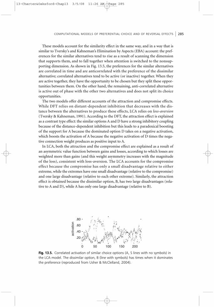
These models account for the similarity effect in the same way, and in a way that issimilar to Tversky’s and Kahneman’s Elimination by Aspects (EBA) account: the pref-erences for the similar alternatives tend to rise as a result of scanning the dimensionthat supports them, and to fall together when attention is switched to the nonsup-porting dimension. As shown in Fig. 13.5, the preferences for the similar alternativesare correlated in time and are anticorrelated with the preference of the dissimilaralternative; correlated alternatives tend to be active (or inactive) together. When theyare active together, they have the opportunity to be chosen but they split these oppor-tunities between them. On the other hand, the remaining, anti-correlated alternativeis active out of phase with the other two alternatives and does not split its choiceopportunities.

The two models offer different accounts of the attraction and compromise effects.While DFT relies on distant-dependent inhibition that decreases with the dis-tance between the alternatives to produce these effects, LCA relies on loss-aversion(Tversky & Kahneman, 1991). According to the DFT, the attraction effect is explainedas a contrast type effect: the similar options A and D have a strong inhibitory couplingbecause of the distance-dependent inhibition but this leads to a paradoxical boostingof the support for A because the dominated option D takes on a negative activation,which boosts the activation of A because the negative activation of D times the nega-tive connection weight produces as positive input to A.

In LCA, both the attraction and the compromise effect are explained as a result ofan asymmetric value function between gains and losses, according to which losses areweighted more than gains (and this weight asymmetry increases with the magnitudeof the loss), consistent with loss-aversion. The LCA accounts for the compromiseeffect because the compromise has only a small disadvantage relative to eitherextreme, while the extremes have one small disadvantage (relative to the compromise)and one large disadvantage (relative to each other extreme). Similarly, the attractioneffect is obtained because the dissimilar option, B, has two large disadvantages (rela-tive to A and D), while A has only one large disadvantage (relative to B).

0

.20

.40

.60

.80

activ

atio

n

50 100 150 200

Fig. 13.5. Correlated activation of similar choice options (A, S lines with no symbols) inthe LCA model. The dissimilar option, B (line with symbols) has times when it dominatesthe preference (reproduced from Usher & McClelland, 2004).


Discussion of computational models and further predictionsBoth of the models described in the previous section can account for the three con-textual reversal effects, promising thus to provide a unified explanation of multi-attribute preferential choice. The models also share many properties (the switch ofattention between dimensions, the leaky integration of the valences or advantages,and the lateral inhibition between the choice units). There are, however, a few basicdifferences in the process by which the reversal effects arise. We focus the discussionon these core differences before turning to a set of predictions.

Non-linearity and value functionsWhereas the DFT is a linear model, there are two types of nonlinearities in the LCAmodel. The first one is the biological constraint that activation cannot turn negative(unlike valences in DFT) and thus there is no ‘excitation by negated-inhibition’. InUsher and McClelland (2004) we have argued that this is an important biological con-straint and Busemeyer and colleagues have responded by suggesting possible biologi-cal implementations of their scheme (Busemeyer et al., 2005). Here we focus on a setof functional considerations.

In Section ‘Perceptual-choice, optimality, and the LCA model’ we reviewed theapplication of the LCA to perceptual choice, showing that its flexible generalisation tomultiple choice (allowing it to maintain high performance at large-n) relies to a largeextent on the zero-threshold nonlinearity, which makes the units that receive littlesupport drop out of the choice process. In a linear system with many options, as islikely to be the case in daily decision-making, the many options that receive little sup-port will become negatively activated and will send noninformative input into the rel-evant choice units, reducing the choice quality. This problem is likely to be exacerbatedif unavailable options are assumed to compete during the choice process, as the DFTneeds to assume to account for reference effects (see below).

The second type of nonlinearity assumed in the LCA but not in DFT involves thenature of the value or utility function. Whereas the DFT has a linear value function,and choice patterns such as loss-aversion are thought to be emergent (or derivative)from the model’s behaviour, in the version of the LCA we used, the value-function isexplicit. To illustrate this distinction, let us examine how the two approaches canaccount for one of the cornerstones of preferential choice: the framing effects (see Fig. 13.2a). In the LCA we are following Tversky in assuming that when the choiceoffers an explicit reference (a present job that is being terminated) the availableoptions are evaluated relative to that reference. Because of the logarithmic nonlinear-ity of the value function, the observers will prefer A from reference Ra, but will prefer B from reference Rb.4 To explain the reference effect, protagonists of the DFT


4 This is the case even without assuming that the value function for losses is steeper than thatfor gains (see Bogacz et al., 2007, section 5 for details). Assuming a steeper value function forlosses will further amplify the effect.


have proposed that the unavailable reference option takes part in the choice process,but is not chosen because it has a low value on a third dimension: the availability; thismakes the reference Ra, somehow similar to the dominated option D (in Fig. 13.2b)and the reference reversal effect is then explained as a contrast effect, similar to theexplanation of the attraction effect. Note, however, that by assuming that unavailableoptions compete for choice, one has to bring in every choice act a potential large set ofunattractive options. As explained above, this is likely (in a linear model) to result in areduction of the choice quality.

In addition to this consideration, we believe that there is independent evidence infavour of nonlinearities in the value function. Consider the task facing the decision-maker in choice options such as those illustrated in Fig. 13.2. To do this one has to repre-sent the magnitudes that correspond to the various alternatives. Since magnitudeevaluation is thought to involve a logarithmic representation and is subject to Weber’slaw,5 it is plausible that it also affects the value functions. This idea is not new. In fact itdates back to Daniel Bernoulli (1738/1954), who proposed a logarithmic type of nonlin-earity in the value function in response to the so-called St. Petersburg paradox, almosttwo centuries ago.6 Bernoulli’s assumption—that internal utility is logarithmicallyrelated to objective value—offers a solution to this paradox and has been included in thedominant theory of risky choice, the prospect theory (Tversky & Kahneman, 1979).Moreover, a logarithmic function, such as log(1+x) starts linearly and then is subject todiminishing returns, which is a good approximation to neuronal input–output responsefunction of neurons at low to intermediate firing rates (Usher & Niebur, 1996).7

In our recent paper (Bogacz et al., 2007) we have explored the consequences ofusing such a logarithmic value function without the assumption of the asymmetrybetween gains and losses (the value for negative x, is then defined as –log(1 – x)). Weshow there that this logarithmic assumption alone can suffice for accounting for someof the reversal effects, such as the reference effect and some aspects of the attractionand the compromise effect. We elaborate here on the latter.

DISCUSSION OF COMPUTATIONAL MODELS AND FURTHER PREDICTIONS 287

5 The Weber law states that to be able to discriminate between two magnitudes (e.g. weights),x and x+dx, the just-noticeable-difference, dx, is proportional to x itself.

6 This paradox was first noticed by the casino operators of St. Petersburg (see for exampleGlimcher, 2004, pp. 188–192 for detailed descriptions of the paradox and of Bernoulli’s solu-tion). Here is a brief description. Consider the option of entering a game, where you areallowed to repeatedly toss a fair coin until ‘head’ comes. If the ‘head’ comes in the first tossyou receive £2. If the ‘head’ comes in the second toss, you receive £4, if in the third toss, £8,and so on (with each new toss needed to obtain a ‘head’ the value is doubled). The question iswhat is the price that a person should be willing to pay for playing this game. The puzzle isthat although the expected value of the game is infinite (E = Σi=1,…, 1/2i 2i = Σi=1,…, 1 = ),as the casino operators in St. Petersburg discovered, most people are not willing to pay morethan £4 for playing the game and very few more than £25 (Hacking, 1980). Most people showrisk-aversion.

7 While neuronal firing rates saturate, it is possible that a logarithmic dependency exists on awide range of gains and losses, with an adaptive baseline and range (Tobler et al., 2005).



The nature of the compromise effectThere are a few issues to examine in understanding why people prefer compromiseoptions. The first explanation, originally offered by Simonson (1989) is that this is theresult of a conscious justification strategy: people choose the compromise becausethey have an easy way to justify it to themselves and to others. Note, however, thatexistence of such a heuristic does not imply that there are no additional factors thatcontribute to the effect. In the following we explore a number of potential contribut-ing factors (on top of the justification heuristics) that emerge from neurocomputa-tional models. The first (non-justificatory) factor, we examine, involves to the way inwhich nonlinear utilities are combined across two or more dimensions. Assuming alogarithmic value function, v(x) = log (1 + x), one can see that when summing acrosstwo dimensions, one obtains: U(x1,x2) = u(x1) + u(x2) = log[1+ (x1 + x2) + x1x2].Figure 13.6 illustrates a contour plot of this 2D utility function.

One can observe that equal preference curves are curved in the x1−x2 continuum:the compromise (0.5,0.5) has a higher utility than the (1,0) or (0,1) options. Whilethis cannot (on its own) account for the compromise effect, which requires a changein the shares of the same two options when a third option in introduced, it still leadsto an interesting prediction. Decision-makers are likely to prefer a middle-rangeoption (0.5, 0.5) to an extreme range one (1-x, x) for 0 < x < 0.5, in binary choice, andthe preference difference should increase the smaller x is (extreme options are lessattractive than middle-range options even in the absence of context). Data supportingthis prediction is presented in the following section.

Contextual contributions can further add to this tendency to choose options in themiddle of the range. Two possibilities arise from the DFT and the LCA models. Accordingto the DFT, the preference for the compromise is due to the dynamically correlated activa-tions (the choice preferences). According to the DFT the preferences of the two extremeoptions are correlated with each other but not with the compromise (because of thestronger inhibition between more similar options) and thus, they split their wins, makingthe compromise option stand out and receive a larger share of choices (Roe et al., 2001).

The process that is responsible for the effect in the LCA model is not correlational,but rather due (as Tversky suggested) to the nature of the nonlinearity and framing invalue evaluations. Consider first, the simple logarithmic nonlinearity described above(without the asymmetry for losses) and note that the value of options defined in a

Fig. 13.6. 2D logarithmicvalue-function, U(x1,x2) = u(x1)+u(x2) = log[1+ (x1+x2) + x1x2]


2D parametric space depends on a reference (see below). If this reference changeswith the choice set, a reversal effect arises. Consider, for example, a trinary choicebetween options: A = (1,0), B=(0.5,0.5), and C = (0,1) and another binary choicebetween options A = (1,0), B = (0.5,0.5). If we assume that decision makers use theminimum value on both dimensions as reference (i.e., (0,0) in the trinary choice and(0.5) in the binary choice, we obtain that decision-makers will be indifferent betweenA and B in binary choice, but they will prefer B (the compromise) in trinary choice(see, Bogacz et al., 2007). Second, the existence of an asymmetric value function,which is steeper in the domain of losses, provides another explanation, without theneed to assume that the reference changes from the binary to the trinary set. In thiscase, all we need to assume is (following Tversky & Simonson, 1993) that decision-makers use each option as a reference to each other option (i.e., they evaluate differ-ences rather than the options themselves). As shown in the previous section, this leadsto a compromise effect because the extremes (but not the compromise) have largedisadvantages that are penalised by the loss-aversive value-function.

In the following, we present some preliminary data that are aimed at testing thesepredictions. The first experiment examines binary and trinary preferences amongoptions defined over two attributes with tradeoffs, by comparing a middle option(both attribute values in middle of the range) with an extreme one (one of the attrib-utes at the high-end and the other one at the low-end). The second experiment,examines the correlational hypothesis. This is done by announcing, immediately afterthe decision-maker has chosen an extreme option, that this option is now unavailableand a speeded choice between the remaining two options has to be made.

Preliminary experimental investigations of the compromise effect

Experiment 1—A parametric study of the value of 2D trade-off optionsThe experiment was conducted on choice between options defined over two dimen-sions with values that create a tradeoff (Fig. 13.7). The aim was to compare the likeli-hood of choosing an alternative with attribute values in the middle of the range,relative to alternatives with extreme values, as a function of the distance between theextremes in the attribute space (small vs. large separation). Two groups of participantswere tested. The first group were tested on trinary choice (Experiment 1A) and thesecond group on binary choice (Experiment 1B).

MethodParticipants. Seventy-eight subjects participated in the trinary study (Experiment

1A) and 28 in the binary choice (Experiment 1B).

DesignThe experiment was within-subjects with two levels: small separation (B,C,D) or

(B,C) versus large separation (A,C,E), or (A,C) as illustrated in Fig. 13.7. The depend-ent variable was the probability of choosing the compromise and the extreme options.

PRELIMINARY EXPERIMENTAL INVESTIGATIONS OF THE COMPROMISE EFFECT 289



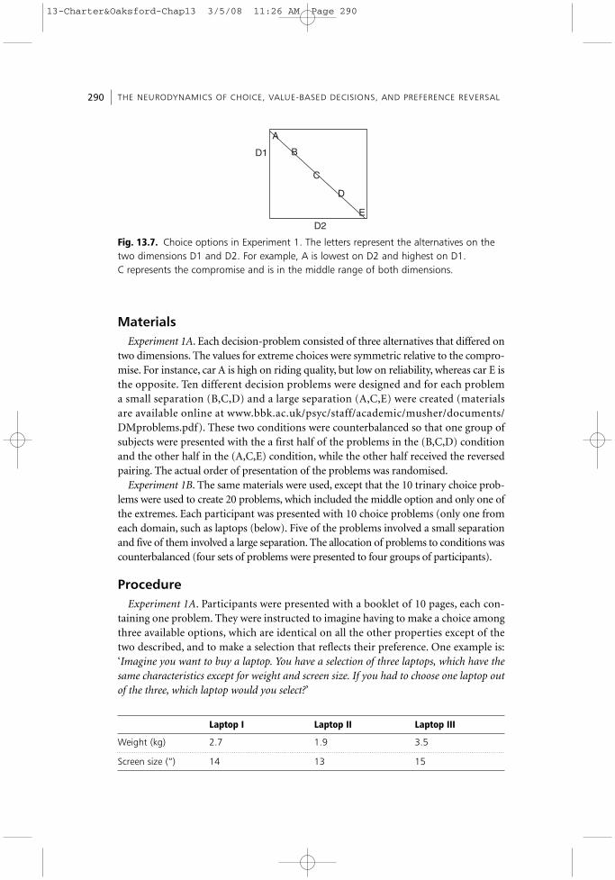
MaterialsExperiment 1A. Each decision-problem consisted of three alternatives that differed on

two dimensions. The values for extreme choices were symmetric relative to the compro-mise. For instance, car A is high on riding quality, but low on reliability, whereas car E isthe opposite. Ten different decision problems were designed and for each problem a small separation (B,C,D) and a large separation (A,C,E) were created (materials are available online at www.bbk.ac.uk/psyc/staff/academic/musher/documents/DMproblems.pdf). These two conditions were counterbalanced so that one group ofsubjects were presented with the a first half of the problems in the (B,C,D) conditionand the other half in the (A,C,E) condition, while the other half received the reversedpairing. The actual order of presentation of the problems was randomised.

Experiment 1B. The same materials were used, except that the 10 trinary choice prob-lems were used to create 20 problems, which included the middle option and only one ofthe extremes. Each participant was presented with 10 choice problems (only one fromeach domain, such as laptops (below). Five of the problems involved a small separationand five of them involved a large separation. The allocation of problems to conditions wascounterbalanced (four sets of problems were presented to four groups of participants).

ProcedureExperiment 1A. Participants were presented with a booklet of 10 pages, each con-

taining one problem. They were instructed to imagine having to make a choice amongthree available options, which are identical on all the other properties except of thetwo described, and to make a selection that reflects their preference. One example is:‘Imagine you want to buy a laptop. You have a selection of three laptops, which have thesame characteristics except for weight and screen size. If you had to choose one laptop outof the three, which laptop would you select?’

A

B

C

D

E

D1

D2

Fig. 13.7. Choice options in Experiment 1. The letters represent the alternatives on thetwo dimensions D1 and D2. For example, A is lowest on D2 and highest on D1. C represents the compromise and is in the middle range of both dimensions.

Laptop I Laptop II Laptop III

Weight (kg) 2.7 1.9 3.5

Screen size (“) 14 13 15


Experiment 1B. The procedure was identical to experiment 1A, except for the fact thatthe participants were emailed the choice problems in a Word-attachment and theysent it back with their marked responses.

ResultsThe fraction of choices for the compromise and the extreme options are shown in Fig. 13.8 (trinary choice: left panel and binary choice right panel), for the small andthe large separation conditions. [In trinary choice (left panel) the extreme conditionswere averaged, thus the normalisation is: 2P(extreme) + P(compromise) =1].

The choice probabilities in trinary choice (Experiment 1A) were analysed using a 2(extreme vs. compromise) by 2 (small vs. large separation) within subjects ANOVA.This yielded a significant main effects of compromise, F(1,77) = 69.84, p < 0.001, andof degree of separation, F(1,77) = 42.066, p < 0.001, and a highly significant interac-tion of compromise vs. degree of separation, F(1,77)=42.066, p < 0.001. This indicatesthat the compromise options receive a higher share than the extreme options and thatthis effect is larger at high separation (by 21%). Interestingly, a similar pattern isfound in the binary choice (Experiment 1B), where participants chose the option (C)(in the middle of the value range) more than the extreme option (B, C, A or E), andthis effect increases at large separations (A, E).

This suggests that the main factor that contributes to the participants’ preference ofthe compromise option is the fact that this option is within the middle of the prefer-ence range, which has a higher 2D-value (Fig. 13.6). It is possible that a further con-textual effect contributes to the compromise effect in trinary choice.8 As the presentexperiments were between-participants (and there were some differences in proce-dure), further experiments are required to evaluate accurately the magnitude of thesecontributions and their dependence on the distance between the extremes. Althoughthis experiment does not distinguish between the LCA/DFT accounts of the compromise


8 This can be computed as P3(C)/[P3(C) + P3(A)] – P2(C)/[ P2 (C) + P2(A)], where P3 and P2are the trinary and binary choice probabilities.

Small separation Large separation0

0.2

0.4

0.6

0.8

1

Small separation Large separation

Pro

bab

ility

of

cho

ice

0

0.2

0.4

0.6

0.8

1

Pro

bab

ility

of

cho

ice

Extreme choice

Compromise choice

Extreme choice

Compromise choice

Fig. 13.8. Proportion of choices in trinary (Experiment 1A; left panel) and in binarychoice (Experiment 1B; right panel). Error bars are SEM.


effect, it suggests that the nonlinearity of the value function is an important contribu-tor of the decision-makers’ preference of middle-range options.

Is the compromise a dynamic correlation effect?If the compromise effect is caused, as predicted by the DFT, by the fact that the prefer-ences of the extremes are correlated in time, it should be possible, in principle, todetect a signature of this correlation. One way to investigate this is by presenting participants with the three-choice compromise option, and in some of the cases,following the participant’s choice, announce that the option chosen is unavailable buta speeded choice is possible (under deadline) for one of the other two options. Theidea is that, if the participant chose one of the extremes in her 1st choice, and if thepreferences of the two extremes are correlated, then at the moment of the response,there should be a high likelihood that the preference of the other extreme is also high (relative to the compromise, which is not correlated). Thus one may predict that theparticipant will choose the 2nd extreme in her 2nd choice, following her 1st choice ofthe other extreme option. One caveat to this prediction is that, following theannouncement of the unavailability of her preferred choice, the participant willrestart the choice from scratch, in which case the advantage of the correlated alterna-tive becomes immaterial. Such restart, however, is expected to lead to longer choicelatencies, leading to a 2nd prediction: the choice latencies of the 2nd response shouldbe faster when the other extreme is chosen than when the compromise is chosen (as inthe latter case a restart is more likely). The LCA model makes the opposite prediction.Here the extreme options are anti-correlated (due to the scan of aspects), whichtogether with the fact that the compromise receives more activation (due to the non-linear value function) leads to a strong preference the compromise when a secondchoice is offered after the first choice (of an extreme option) is announced as unavailable.

MethodParticipants. One hundred and forty-three participants volunteered to take part in

this experiment (60% females; age-range 20–61 with a mean of 37).

MaterialsThe material consisted of 30 choice problems with three alternatives that varied on

two dimensions, of a similar type to those shown in Table 13.1. Out of these problems,25 were of the compromise form. Of those, 14 had a 2nd choice required afterannouncing the unavailability of the 1st chosen option. (The other 11 did not involveunavailable options so as not to create a strategy that prepares the two preferredoptions in advance.) A table that includes those 25 problems is available on:www.bbk.ac.uk/psyc/staff/academic/musher/documents/DMproblems.pdf

ProcedureThe experiment was run on the web, using the ‘express’ psychology experiments

package (Yule & Cooper 2003), which recorded the responses and the latencies.



The participants were instructed to imagine the situations described, as real choicesituations they encounter in daily life and to indicate their preference. They were alsoinstructed that sometimes (as in real life) an option they chose may be unavailableand that in such a case they will be able to make a 2nd choice (it was emphasized thatthis 2nd choice should be fast).

ResultsThe fraction of choices in favour of the compromise and extreme options (out

of 14) in the 1st choice made is shown in Fig. 13.9 (left panel).One can see (left panel) that, consistent with the data from Experiment 1, the par-

ticipants chose the compromise option more than they chose the extreme options(t(142) = 7.185, p < 0.001). The fraction of choices made after a first choice, whichwas an extreme option announced to be unavailable is shown in the right panel. Onecan see that in such a situation the participants chose more than 90% the compromiseoption (t(142) = 35.354, p < 0.001).

Finally, we examine the response latencies of these 2nd choices and compare thelatency of choosing the compromise over the extreme. As shown in Fig. 13.9 (right),the probability of choosing the extreme is less than 10% (only 58 participants out ofthe 143 made such choices, so we could only compare reaction time data for them).Although most of the responses were faster than 7 sec, indicating the participants fol-lowed the instructions of making a speeded response (this time includes the readingof the un-availability), there are also some slow RTs, that are as long as 30 sec.Eliminating such outliers (10 out of about 2000 in the whole data set), one finds thatthe average choice is significantly faster in the compromise 2nd choice (4.3 sec), thanin the extreme 2nd choice (6.3 sec), t(57) = 4.092, p < 0.001. The full RT density-distributions (collapsed over all the participants) for the compromise (blue) and theextreme 2nd choices is shown in Fig. 13.10 (left). One can observe that extremechoices are slower in their mode and have a longer tail. This is consistent with RT-datafrom individual participants (right panel), which show slower responses for extreme(green) than to compromise (red) 2nd choices.


0

0.2

0.4

0.6

0.8

1

Compromise Extreme

Pro

bab

ility

of

cho

ice

0

0.2

0.4

0.6

0.8

1

Pro

bab

ility

of

cho

ice

Compromise2nd choice

Fig. 13.9. The probability to choose the compromise and the extreme options in thefirst choice opportunity (left), and to choose compromise/extreme in the second choice.


This result does not support the correlational hypothesis of the compromise effect,however, one cannot totally rule out such an account, because one can explain thepreference for the compromise in the 2nd choice, within the DFT (J. Busemeyer, per-sonal communication), by assuming that once an option becomes unavailable it actsas a dominated decoy and enhances the likelihood to chose the compromise (which ismore similar with it), as in the attraction effect. Further studies, which contrast themagnitude of the compromise effect in situations where the extremes are available orunavailable, could help to test this proposal.

General discussionIn this chapter, we have examined how the LCA model, which was originally devel-oped to account for perceptual choice, can be extended to preferential choice betweenalternatives that vary on several dimensions or attributes (see Stewart & Simpson, thisvolume, for a model of risky choice that treats probability and value as independentdimensions, and makes decisions on the basis of integrated comparisons). The LCA isa neurocomputational model, from a similar family with the DFT. As such, they sharea similar approach, and vary on a number of important but secondary mechanisms.In the previous sections we discussed the differences between the LCA and the DFTaccounts to preference reversal and we suggested possible ways to examine them.9

Here we highlight their common approach by contrast with heuristic approaches(LeBoef & Shafir, 2005; Todd & Gigerenzer, 2000; Gigerenzer 2006) and we brieflyaddress some implications to the debate on rationality in human choice.

Neucomputational models vs. heuristicsIt is customary to understand choice heuristics as algorithms that are not optimal, butwhich can produce fast and reasonable choices for given situations (Gigerenzer, 2000,2006). Understood in this minimal way, neurocomputational models such as DFT and


−0.05

0

0.05

0.1

0.15

0.2

0.25

0.3

0 10 15 20 25

1000 2000

5000 10000

3000RT [ms]

RT [ms]

30

Reaction time (sec)

Pro

bab

ility

Extreme toCompromiseExtreme toExtreme

5

Fig. 13.10. Response latencies for 2nd choices in Experiment 2. Left: RT density-distribution of all responses of 58 participants; Right: RTs of two participants.

9 The LCA is more similar in its approach with the decision-by-sample model (Stewart, thisvolume), but they vary on their assumptions about the order of attentional switches (betweenattributes in the LCA) and between alternatives first, in the decision-by-sample).


LCA are heuristics, as they indeed can produce reasonable and fast choices. There is,nevertheless, a feeling that something distinguishes these models from typical heuristics.We believe that the main contrast between the two resides in the nature of the algo-rithm. While the typical heuristics involve rules that can be verbally formulated in apropositional format and which have a sequential nature, the neurocomputationalalgorithms are mathematical rather than propositional and they involve some degreeof parallel (rather than sequential) processing. This stems from the distinctionbetween parallel distributed processes (PDP) and symbolic ones, which has been dis-cussed in detail in other domains of cognition (McClelland et al., 1986; Rumelhart et al.,1986). In the light of this distinction, a number of considerations need to be addressed[see further discussion in the BBS replies to Todd and Gigerenzer (2000), in particu-lar: Chater, 2000; Cooper, 2000; Oaksford, 2000; Shanks & Lagnado, 2000].

The LCA approach relies on some elements of prospect theory, in particular theform of the value function and loss-aversion. In their recent heuristic proposal topreferential choice under risk, the priority heuristic, Brandstatter et al. (2006) argueagainst the various variants of the prospect theory on several grounds. First, theymaintain that all weighing models based on Bernoulli type corrections of the EV prin-ciple (such as prospect theory) are overly complex, as they rely on all the informationavailable and require both summations and multiplications. Second, they suggest thatheuristics, but not the prospect theory, provides a process model of preference. Third,they argue that such heuristics are ecologically rational and that, therefore, the so-called ‘violations of rationality’ are a misleading outcome of our over-reliance onunrealistic EV-type rationality norms. While we are sympathetic to the rational-ecological approach, we believe that the use of mathematically defined value func-tions (a la Bernoulli) within neurocomputational process models can achieve morethan the use of disparate verbal heuristics, on all the three grounds.

Consider simplicity considerations first. On the one hand, while weighing modelsare complex from a symbolic perspective (where one actually multiplies and adds val-ues) they are not so within a PDP one, as there is nothing more straightforward thancomputing weighted averages that implement EV (see Figs. 13.3 and 13.4)10 and aslogarithmic nonlinearities come for free (they are assumed anyway within basic psy-chophysical principles of magnitude evaluations, such as Weber’s law). On the otherhand, there is complexity hidden in the symbolic form of some heuristics, whichrequire fundamentally different computations for different problems within the samedomain. As an example, the priority heuristic (a lexicographic type heuristic) requiresdifferent computations for choices between options that differ in EV (thus some com-putation of EV needs to be done anyway) and for gains vs. losses.11 Similarly, one can

GENERAL DISCUSSION 295

10 In fact we face the inverse puzzle: what are the processes that limit a straightforward EV com-putation.

11 The rationale stated for the priority heuristic is that the first concern is the lowest possibleoutcome (i.e., the lowest gain). By this principle, the first concern in the domains of lossesshould be the highest possible loss, rather than the lowest one as the heuristics assumes toaccount for loss-aversion. In terms of complexity this assumption is not simpler thanprospect’s theory asymmetry of value functions for gains and losses.


explain the preference reversal effects in 2D attribute choice with verbal heuristics ofthe type: in a compromise choice, choose the middle option, but in a similarity situa-tion choose the different (extreme) option. As there is a continuity of choice optionsover the 2D attribute space, one has to decide when to switch from one version of theheuristic to the other; this seems thus to require a meta-model to decide on theheuristic to use. We believe that a neurocomputational approach that employs contin-uous functions has a better prospect of obtaining a unified account of preference.Moreover, in some conditions, such a model may be approximately described by a verbal heuristic. For example, the LCA has some properties in common with the EBAheuristic (the shift of attention from attribute to attribute) and one of its neural pre-cursors (Usher & Zakay, 1993) was shown to extrapolate among a large number ofheuristics in multi-attribute choice.

Second, the neural models are in essence process models, which make dynamic pre-dictions (Usher & McClelland, 2004). While such models can obtain fast and reason-able choices like the verbal heuristics, they can also do something that, paradoxically,heuristics don’t do but people (unfortunately) do: vacillate and procrastinate in theirdecision! For example, unlike lexicographic type heuristics, models such as LCA andDFT vacillate in their preferences. One interesting possibility is that neurocomputa-tional models, of the type discussed here, are at the interface between purely con-scious (rule based and capacity limited) lexicographic type of decision-making andintuitive/gut-feeling type of choices, which are not subject to the capacity limitationsof conscious thought and are able to weigh large number of attributes in parallel(Dijksterhuis & Nordgren, 2006). Finally, we examine a few considerations on opti-mality and rationality principles.

Optimality and rationalityThe domain of multi-attribute preference does not possess an external criterion forthe value (or quality) of choice. Nevertheless, some of its ingredients, the leaky inte-gration, the logarithmic value function, and the loss-aversion, can be interpreted inrelation to adaptive principles.

In Section ‘Perceptual-choice, optimality, and the LCA model’, we summarisedanalysis that indicates optimal performance in choice under stationary conditions,when leak and inhibition are perfectly balanced. Our own experiments in perceptualchoice (Usher & McClelland, 2001) and those by Hertwig et al. (2004) in feedback-driven value decisions, indicate that some participants show a recency bias (leak dom-inance) that results in suboptimality. One interesting possibility is that thissuboptimality is the cost one needs to pay for enabling agents to maintain sensitivityto changes in their environment (Daw et al., 2006)—a type of the exploitation/explo-ration tradeoff. Consider next the 2D value function (Fig. 13.6), which results in pref-erence for middle-of-the-range options. This value function involves a combinationof linear and multiplicative terms. The inclusion of a multiplicative term in the utilityoptimization is supported by a survival rationale: to survive animals need to ensurethe joined (rather than separate) possession of essential resources (like food andwater). In addition, the higher slope of the value function for losses (relative to gains)



can be justified by the ‘asymmetry between pleasure and pain’ (Tversky & Kahneman,1991). This, in turn, could be an adaptive outcome of the fact that preventing losses ismore critical for survival than getting gains (a single large loss can be critical; attain-ing large gains is not).

As task optimality is environment-dependent, an important insight is that rationalstrategies of choice require the flexibility to modify the choice parameters in responseto the environment and demands (under some situations inhibition dominance or lin-ear value function are advantageous). Such flexibility, however, may be subject to limi-tations. Unlike Gigerenzer and colleagues (but like Tversky and Kahaneman, 2000;Kahaneman, 2003), we think that contextual reversal effects of the type discussed heredemonstrate a limitation of rationality in choice preference. After all, intransitive pref-erences and contextual reversals can be used to manipulate agents’ choice and eventransform them into money pumps; even if we evolved within a different environ-ment, it is rational to do well in the present one. The notion of rationality, requiringflexible responses to the present environment/tasks, should not be diluted to a fixedrepertoire of strategies adaptive to past environments and tasks. The power of choicemodels is to account for the sources of the adaptive powers of decision-makers andtheir limitations, and equally important to quantify the degree of these limitations12

and find ways to eliminate them. A recent suggestion that requires further investigationis that one can overcome limitations in the ability to integrate across dimensions byrelying on intuitive13/implicit decion-making (Dijksterhuis, et al, 2006).

Acknowledgments Thanks are due to Claudia Sitz and Yvonne Lukaszewicz for running participants inExperiments 1–2, and to David Lagnado for a critical reading.

ReferencesBarnard, G. (1946). Sequential tests in industrial statistics. Journal of Royal Statistical Society

Supplement, 8, 1–26.296

Bernoulli, D. (1738/1954). Exposition of a new theory on the measurement of risk.Ekonometrica, 22, 23–36.

Bogacz, R., Usher, M., Zhang, J., & McClelland J. L. (2007). Extending a biologically inspiredmodel of choice: Multi-alternatives, nonlinearity and value-based multidimensional choice.Philosophical Transactions of the Royal Society, B (in press).

Brandstätter, E., Gigerenzer, G., & Hertwig, R. (2006). The priority heuristic: Making choiceswithout trade-offs. Psychological Review, 113, 409–432.

Britten, K. H., Shadlen, M. N., Newsome, W. T., & Movshon, J. A. (1993). Responses of neuronsin macaque MT to stochastic motion signals. Visual Neuroscience, 10(6), 1157–1169.

REFERENCES 297

12 In this regard, lexicographic type models are the worse off. Fortunately, only a minority of humanparticipants exhibit intransitive preferences as predicted by such models (Tversky, 1969).

13 But see Slovic et al. (2004), for an insightful discussion of the limitations and dangers of intu-itive/affective preferential choice.


Busemeyer, J. R., & Johnson, J. G. (2003). Computational models of decision making. In D. Koehler & N. Harvey (Eds.), Handbook of judgment and decision making. BlackwellPublishing Co (To appear).

Busemeyer, J. R., & Diederich, A. (2002). Survey of decision field theory. Mathematical SocialSciences, 43, 345–370.

Busemeyer, J. R., Townsend, J. T., Diederich, A., & Barkan, R. (2005). Contrast effects or lossaversion? Comment on Usher and McClelland (2004). Psychological Review, 111, 757–769.

Chater, N. (2000). How smart can simple heuristics be? Behavioural and Brain Sciences, 23,745–746.

Cooper, R. (2000). Simple heuristics could make us smart; but which heuristic do we applywhen? Behavioural and Brain Sciences, 23, 746–747.

Daw, N. D., O’Doherty, J. P., Dayan, P., Seymour, B., & Dolan, R. J. (2006). Cortical substratesfor exploratory decisions in Humans. Nature, 441, 876–879.

Diederich, A. (1997). Dynamic stochastic models for decision making under time constraints.Journal of Mathematical Psychology, 41, 260–274.

Dijksterhuis, A., Bos, M. W., Nordgren, L. F., & Baaren, R. B. (2006). On making the rightchoice: The deliberation without-attention effect. Science, 311, 1005–1007.

Dijksterhuis, A., & Nordgren, L. F. (2006). A theory of unconscious thought. Perspectives onPsychological Science, 1, 95–109.

Gigerenzer, G. (2006). Bounded and rational. In R. J. Stainton (Ed.), Contemporary debates incognitive science (pp. 115–133). Oxford, UK: Blackwell.

Glimcher, P. W. (2004). Decisions, uncertainty, and the brain: The science of neuroeconomics.Cambridge, MA: MIT Press.

Gold, J. I., & Shadlen, M. N. (2002). Banburismus and the brain: Decoding the relationshipbetween sensory stimuli, decisions, and reward. Neuron, 36(2), 299–308.

Hacking, I. (1980). Strange expectations. Philosophy of Science, 47, 562–567.

Hertwig, R., Barron, G., Weber, E. U., & Erev, I. (2004). Decisions from experience and theeffect of rare events in risky choice. Psychological Science, 15, 534–539.

Huber, J., Payne, J. W., & Puto, C. (1982). Adding asymmetrically dominated alternatives:Violations of regularity and the similarity hypothesis. Journal of Consumer Research, 9,90–98.

Kahneman, D. (2003). Maps of bounded rationality: Psychology for behavioral economics. TheAmerican Economic Review, 93, 1449–1475.

Kahneman, D., & Tversky, A. (1979). Prospect theory: An analysis of decision making underrisk. Econometrica, XLVII, 263–291.

Kahneman, D., & Tversky, A. (Eds.). (2000). Choices, values and frames. Cambridge: CambridgeUniversity Press.

Knetch, J. L. (1989). The endowment effect and evidence of nonreversible indifference curves.American Economic Review, 79, 1277–1284.

Laming, D. R. J. (1968). Information theory of choice reaction time. New York: Wiley.

LeBoef, R., & Shafir, E. B. (2005). Decision-making. In K. J. Holyoak & R. G. Morisson (Eds.),Cambridge handbook of thinking and reasoning. Cambridge: Cambridge University Press.

McClelland, J. L., Rumelhart, D. L., & the PDP Research Group. (1986). Parallel distributed processing: Explorations in the microstructure of cognition (Vol. 2). Cambridge, MA:MIT Press.

Oaksford, M. (2000). Speed, frugality and the empirical basis of take-the-best. Behavioural andBrain Sciences, 23, 760–761.



Roe, R. M., Busemeyer, J. R., & Townsend, J. T. (2001). Multi-alternative decision field theory:A dynamic connectionist model of decision-making. Psychological Review, 108, 370–392.

Rumelhart, D. L., McClelland, J. L., & the PDP Research Group. (1986). Parallel distributed processing: Explorations in the microstructure of cognition (Vol. 1). Cambridge, MA: MITPress.

Samuelson, W., & Zeckhauser, R. (1988). Status quo bias in decision making. Journal of Riskand Uncertainty, 1, 7–59.

Schall, J. D. (2001). Neural basis of deciding, choosing and acting. Nature Reviews.Neuroscience, 2(1), 33–42.

Shadlen, M. N., & Newsome, W. T. (2001). Neural basis of a perceptual decision in the parietalcortex (area LIP) of the rhesus monkey. Journal of Neurophysiology, 86(4), 1916–1936.

Shanks, D. R., & Lagnado, D. (2000). Sub-optimal reasons for rejecting optimality. Behaviouraland Brain Sciences, 23, 761–762.

Simonson, I. (1989). Choice based on reasons: The case of attraction and compromise effects.Journal of Consumer Research, 16, 158–174.

Slovic, P. (1995). The construction of preference. American Psychologist, 50, 364–371.

Slovic, P., Finucane, M. L., Peters, E., & MacGregor, D. G. (2004). Risk as analysis and risk asfeelings: Some thoughts about affect, reason, risk, and rationality. Risk Analysis, 24(2), 311–322.

Smith, P. L., & Ratcliff, R. (2004). Psychology and neurobiology of simple decisions, Trends inNeurosciences, 27(3), 161–168.

Sugrue, L. P., Corrado, G. S., & Newsome, W. T. (2004). Matching behavior and the representa-tion of value in the parietal cortex. Science, 304(5678), 1782–1787.

Sugrue, L. P., Corrado, G. S., & Newsome, W. T. (2005). Choosing the greater of two goods:neural currencies for valuation and decision making. Nature Review and Neuroscience, 6(5),363–375.

Tobler, P. N., Fiorillo, C. D., & Schultz, W. (2005). Adaptive coding of reward value bydopamine neurons. Science, 307(5715), 1642–1645.

Todd, P. M., & Gigerenzer, G. (2000). Precis of Simple heuristics that make us smart. Behavioraland Brain Sciences, 23, 727–780.

Tversky, A. (1972). Elimination by aspects: A theory of choice. Psychological Review 79, 281–299.

Tversky, A., & Kahneman, D. (1979). Prospect theory: An analysis of decision under risk.Econometrica, 47, 263–292.

Tversky, A., & Kahneman, D. (1991). Loss aversion in riskless choice: A reference-dependentmodel. The Quarterly Journal of Econometrics, 106, 1039–1061.

Tversky, A., & Simonson, I. (1993). Context-dependent preferences. Management Science, 39,1179–1189.

Usher, M., & McClelland, J. L. (2001). The time course of perceptual choice: The leaky, competingaccumulator model. Psychological Review, 108(3), 550–592.

Usher, M., & McClelland, J. L. (2004). Loss aversion and inhibition in dynamical models ofmultialternative choice. Psychological Review, 111, 759–769.

Usher, M., & Niebur, N. (1996). Modeling the temporal dynamics of it neurons in visual search:A mechanism for top-down selective attention. Journal of Cognitive Neuroscience, 8,311–327.

Usher, M., & Zakay, D. (1993). A neural network model for attribute based decisions processes.Cognitive Science, 17, 349–396.

REFERENCES 299


Yule, P., & Cooper, R. P. (2003): Express: A web-based technology to support human and computational experimentation. Behavior Research Methods, Instruments, & Computers,35, 605–613.

Vickers, D. (1979). Decision processes in perception. New York: Academic Press.

Wald, A. (1947). Sequential analysis. New York: Wiley.



The neurodynamics of choice, value-based decisions, and preference...

Documents

Transcript of The neurodynamics of choice, value-based decisions, and preference...