The Need for Causal, Explanatory Models in Risk Assessment 2 The need for causa… · The Need for...

31

2The Need for Causal, Explanatory Models in Risk Assessment

2.1 Introduction

The aim of this chapter is to show that we can address some of the core limitations of the traditional statistical approaches exposed in Chapter 1 by introducing causal explanations into the modeling process. The causal models are examples of Bayesian Networks (BNs).

Although we will not formally define BNs until Chapter 5 (because such a definition requires an understanding of Bayesian probability that we explain in Chapter 4), our intention here is to provide a flavor of their power and flexibility in handling a range of risk-assessment problems.

In Section 2.2 we use the automobile crash example from Chapter 1 to explain the need for and structure of a causal BN. In Section 2.3 we explain why popular methods of risk assessment (such as risk registers and heat maps) are insufficient to properly handle risk assessment. We describe the causal approach to risk assessment in Section 2.4, showing how it overcomes the limitations of the popular methods.

2.2 Are You More Likely to Die in an Automobile Crash When the Weather Is Good Compared to Bad?

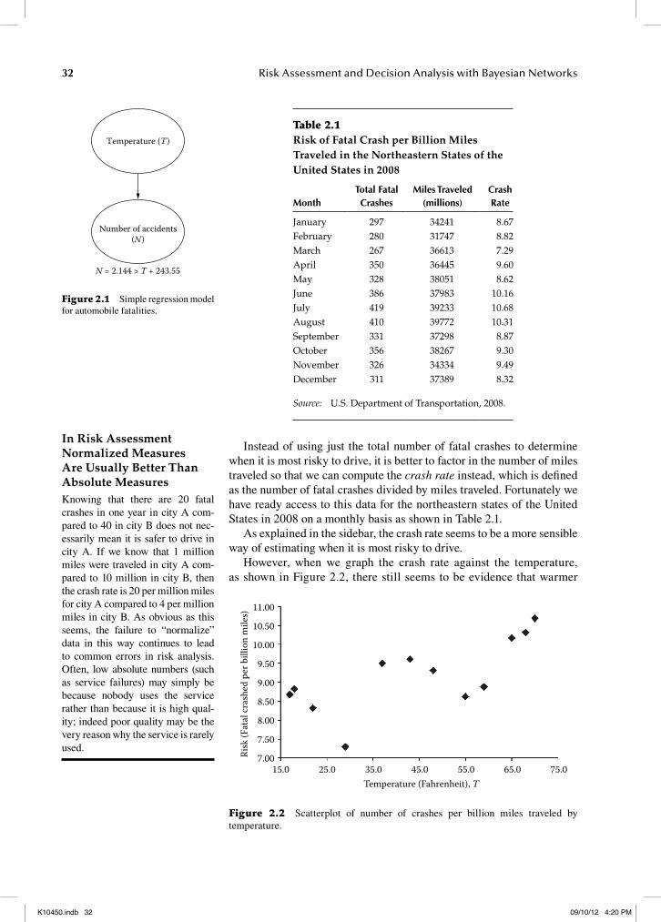
We saw in Chapter 1, Section 1.4 some data on fatal automobile accidents. The fewest fatal crashes occur when the weather is at its worst and the high-ways are at their most dangerous. Using the data alone and applying the standard statistical regression techniques to that data we ended up with the simple regression model shown in Figure 2.1.

But there is a grave danger of confusing prediction with risk assess-ment. For risk assessment and management the regression model is use-less, because it provides no explanatory power at all. In fact, from a risk perspective this model would provide irrational, and potentially danger-ous, information. It would suggest that if you want to minimize your chances of dying in an automobile crash you should do your driving when the highways are at their most dangerous, in winter.

Visit www.bayesianrisk.com for your free Bayesian network software and models in this chapter

We discuss a simplified view of risk assessment and do not cover decision and utility theory except in passing and to make the point that such theory is not enough without coherent models of the problem situation. Most other books try to present decision the-ory and risk all at once and in a very mathematical way; this can be rather overwhelming.

K10450.indb 31 09/10/12 4:20 PM

32 Risk Assessment and Decision Analysis with Bayesian Networks

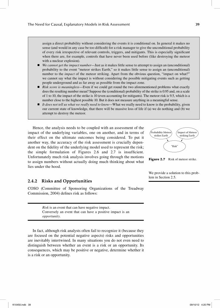
Instead of using just the total number of fatal crashes to determine when it is most risky to drive, it is better to factor in the number of miles traveled so that we can compute the crash rate instead, which is defined as the number of fatal crashes divided by miles traveled. Fortunately we have ready access to this data for the northeastern states of the United States in 2008 on a monthly basis as shown in Table 2.1.

As explained in the sidebar, the crash rate seems to be a more sensible way of estimating when it is most risky to drive.

However, when we graph the crash rate against the temperature, as shown in Figure 2.2, there still seems to be evidence that warmer

In Risk Assessment Normalized Measures Are Usually Better Than Absolute MeasuresKnowing that there are 20 fatal crashes in one year in city A com-pared to 40 in city B does not nec-essarily mean it is safer to drive in city A. If we know that 1 million miles were traveled in city A com-pared to 10 million in city B, then the crash rate is 20 per million miles for city A compared to 4 per million miles in city B. As obvious as this seems, the failure to “normalize” data in this way continues to lead to common errors in risk analysis. Often, low absolute numbers (such as service failures) may simply be because nobody uses the service rather than because it is high qual-ity; indeed poor quality may be the very reason why the service is rarely used.

Temperature (T)

Number of accidents(N)

N = 2.144 > T + 243.55

Figure 2.1 Simple regression model for automobile fatalities.

11.00

10.50

10.00

9.50

9.00

8.50

8.00

7.50

Risk

(Fat

al cr

ashe

d pe

r bill

ion

mile

s)

7.0015.0 25.0 35.0 45.0

Temperature (Fahrenheit), T55.0 65.0 75.0

Figure 2.2 Scatterplot of number of crashes per billion miles traveled by temperature.

Table 2.1Risk of Fatal Crash per Billion Miles Traveled in the Northeastern States of the United States in 2008

MonthTotal Fatal Crashes

Miles Traveled (millions)

Crash Rate

January 297 34241 8.67February 280 31747 8.82March 267 36613 7.29April 350 36445 9.60May 328 38051 8.62June 386 37983 10.16July 419 39233 10.68August 410 39772 10.31September 331 37298 8.87October 356 38267 9.30November 326 34334 9.49December 311 37389 8.32

Source: U.S. Department of Transportation, 2008.

K10450.indb 32 09/10/12 4:20 PM


weather is “riskier” (although the correlation is weaker than when we considered simply the total number of fatal crashes).

Since common sense suggests that we should expect the risk to increase during winter (when road conditions are most dangerous) we must look elsewhere for an explanation.

What we know is that, in addition to the number of miles traveled (i.e., journeys made), there are other underlying causal and influential factors that might do much to explain the apparently strange statistical observations and provide better insights into risk. With some common sense and careful reflection we can recognize the following:

◾ The temperature influences the highway conditions (they will be worse as the temperature decreases).

◾ But temperature also influences the number of journeys made; people generally make more journeys in spring and summer, and will generally drive less when weather conditions are bad. This then means the miles traveled will be less.

◾ When the highway conditions are bad people tend to reduce their speed and drive more slowly. So highway conditions influ-ence speed.

◾ The actual number of crashes is influenced not just by the number of journeys but also the speed. If relatively few people are driving and taking more care, we might expect fewer fatal crashes than we would otherwise experience.

The influence of these factors is shown in Figure 2.3, which is an example of a BN. To be precise, it is only the graphical part of a BN.

Temperature(T)

Drivingconditions (D)

Number ofaccidents (N)

Drivingspeed (S)

Number ofmiles (M)

Risk ofaccident (R)

Figure 2.3 Causal model for fatal crashes.

K10450.indb 33 09/10/12 4:20 PM


To complete the BN model we have to specify the strength of the rela-tionships between linked factors, since these relationships are gener-ally uncertain. It turns out we need probabilities to do this (we actually need a probability table for each of the nodes). The details of what this all means are left until Chapter 5. But you do not need to know such details to get a feel for the benefits of such a model. The crucial mes-sage here is that the model no longer involves a simple single causal explanation; instead it combines the statistical information available in a database (the objective factors as explained in the sidebar) with other causal subjective factors derived from careful reflection.

The objective factors and their relations are shown with solid lines and arrows in the model, and the subjective factors are shown using dot-ted lines. Furthermore, these factors now interact in a nonlinear way that helps us to arrive at an explanation for the observed results. Behavior, such as our natural caution to drive slower when faced with poor road conditions, leads to lower accident rates. Conversely, if we insist on driv-ing fast in poor road conditions then, irrespective of the temperature, the risk of an accident increases and so the model is able to capture our intuitive beliefs that were contradicted by the counterintuitive results from the simple regression model.

We could extend this process of identifying and attributing causes to help explain the change in risk to include other factors, such as increased drunk driving during the summer and other holiday seasons. This is shown in Figure 2.4.

The role played in the causal model by driving speed reflects human behavior. The fact that the data on the average speed of automobile drivers was not available in a database explains why this variable, despite

In the highway example we have information in a database about tem-perature, number of fatal crashes, and number of miles traveled. These are therefore often called objective factors. If we wish our model to include factors for which there is no readily available infor-mation in a database we may need to rely on expert judgment. Hence, these are often called subjective fac-tors. Just because the driving speed information is not easily available does not mean it should be ignored. Moreover, in practice (as we shall see in Chapter 3) the distinction between what is objective and what is subjective can be very blurred.

People are known to adapt to the perception of risk by tuning the risk to tolerable levels. For exam-ple, drivers tend to reduce their speed in response to bad weather. This is formally referred to as risk homeostasis.

Temperature(T)Driving

conditions (D)

Number ofaccidents (N)

Driving underin�uence (I)

Drivingspeed (S)

Number ofmiles (M)

Risk ofaccident (R)

Figure 2.4 Extended causal model for fatal highway crashes.

K10450.indb 34 09/10/12 4:20 PM


its apparent obviousness, did not appear in the statistical regression model.

By accepting the naïve statistical model we are asked to defy our senses and experience and actively ignore the role unobserved factors play in the model. In fact, we cannot even explain the results without recourse to fac-tors that do not appear in the database. This is a key point: With causal models we seek to dig deeper behind and underneath the data to explore richer relationships than might be admitted by oversimplistic statistical models. In doing so we gain insights into how best to control risk and uncertainty. The original regression model, based on the idea that we can predict automobile crash fatalities based on temperature, fails to answer the substantial question: How can we control or influence behavior to reduce fatalities? This at least is achievable; control of weather is not.

2.3 When Ideology and Causation Collide

One of the first things taught in an introductory statistics course is that correlation is not causation. As we have seen, a significant correlation between two factors A and B (where, for example A is yellow teeth and B is cancer) could be due to pure coincidence or to a causal mechanism such that:

a. A causes B b. B causes A c. Both A and B are caused by C (where in our example C might

be smoking) or some other set of factors.

The difference between these possible mechanisms is crucial in interpreting the data, assessing the risks to the individual and society, and setting policy based on the analysis of these risks. However, in practice causal interpretation can collide with our personal view of the world and the prevailing ideology of the organization and social group, of which we will be a part. Explanations consistent with the ideological viewpoint of the group may be deemed more worthy and valid than others, irrespective of the evidence. Discriminating between possible causal mechanisms a, b, and c can only formally be done if we can intervene to test the effects of our actions (normally by experimentation). But we can apply commonsense tests of causal interaction to, at least, reveal alternative explanations for correlations.

Box 2.1 provides an example of these issues at play in the area of social policy, specifically regarding the provision of prenatal care.

The situation whereby a statistical model is based only on available data, rather than on reality, is called conditioning on the data. This enhances convenience but at the cost of accuracy.

Box 2.1 The Effect of Prenatal Care Provision: An Example of Different Causal Explanations According to Different Ideological Viewpoints

Thomas Sowell (1987) cites a study of mothers in Washington, DC. The study found a correlation between pre-natal care provision and weight of newborn babies. Mothers receiving low levels of prenatal care were dispro-portionately black and poor. Sections of the U.S. media subsequently blamed society’s failure to provide enough prenatal care to poor black women and called for increased provision and resources. They were using a simple

K10450.indb 35 09/10/12 4:20 PM


Simplistic causal explanations (such as the liberal perspective in Box 2.1) are usually favored by the media and reported unchallenged and taken as axiomatic. This is especially so when the explanation fits the established ideology, helping to reinforce ingrained beliefs. Picking apart oversimplistic causal claims and deconstructing and reconstruct-ing them into a richer, more realistic causal model helps separate ide-ology from reality and determines whether the evidence fits reality. The richer model may also help identify more effective possible policy interventions.

Another example where ideology and causation collide is in the so-called conspiracy of optimism explained in Box 2.2.

The time spent analyzing risks must be balanced by the short-term need to take action and the magnitude of the risks involved. Therefore, we must make judgments about how deeply we model some risks and how quickly we use this analysis to inform our actions. There is a trade-off between efficiency and thoroughness here, called the efficiency-thoroughness trade-off (ETTO) (coined by Hollnagel, 2009): too much

causal explanation: lack of prenatal care provision causes low birth weight with consequent detrimental effects on infant health. However, a closer look at the data revealed that, independently of race and income, smoking and alcohol use were respectively twice and six times more prevalent among mothers who did not get prenatal care support. Sowell argues that smoking and alcohol abuse are symptoms of another factor not addressed in the study—personal responsibility. Among mothers who did not smoke or drink alcohol, there was no correlation between prenatal care provision and birth weight. A deficit in personal responsibility could explain the failure to seek prenatal care and also explain the increased propensity to smoke and drink alcohol.

Clearly ideology plays a role in these explanations. What might be characterized as the liberal perspective will tend to blame the problem on an absence of state provision of prenatal care, whereas the conservative per-spective looks for an explanation based on individual behavior and personal responsibility. Figure 2.5 shows the difference in causal model from these two perspectives.

Birth weight

(a) (b)

Prenatal careprovision

Alcohol use Smoking

Birth weight

Prenatal caretake up

Mother personalresponsibility

Prenatal careprovision

Figure 2.5 Ideological perspectives and their causal claims as applied to prenatal care provision. (a) Liberal. (b) Conservative.

K10450.indb 36 09/10/12 4:20 PM


analysis can lead to inaction and inefficiency, and too little analysis can lead to inefficient actions being undertaken.

Consider, for example, a doctor attempting a diagnosis. The doctor may be tempted to undertake many diagnostic tests, at considerable expense but for little additional certainty. In the meantime the disease may progress and kill the patient. The doctor has purchased near cer-tainty but at a devastating cost. Trade-offs such as these are made all of the time but the challenge is to be explicit about them and search for better options.

2.4 The Limitations of Common Approaches to Risk Assessment

The previous sections provided some insight into both why standard statistical techniques provide little help when it comes to risk assess-ment and why causal models (BNs) help. In this section we show that when it comes to quantifying risk, again, the traditional techniques are fundamentally flawed, while BNs provide an alternative solution. This section uses some terms from probability that we will define properly in Chapters 3 and 4, so do not worry too much if there are some things you do not fully understand on first reading. You should still get the gist of the argument.

2.4.1 Measuring Armageddon and Other Risks

By destroying the meteor in the film Armageddon, Bruce Willis saved the world. Both the chance of the meteor strike and the consequences of such a strike were so high, that nothing much else mattered except to try to prevent the strike. In popular terminology what the world was con-fronting (in the film) was a truly massive risk.

But if the NASA scientists in the film had measured the size of the risk using the standard approach in industry they would quickly have discovered such a measure was irrational, and it certainly would not have explained to Bruce Willis and his crew why their mission made sense. Bruce takes to space.

Box 2.2 The Conspiracy of OptimismThe conspiracy of optimism refers to a situation in which a can-do attitude, where action is favored to the exclusion of risk analysis, leads to the underestimation of risk. A classical example of this occurs in tender bids to supply a new system to a disengaged customer who has not taken the care to identify his needs. A bidder that points out the risks and takes a realistic approach is likely to lose the tender to a competitor that shows a positive attitude and plays down future problems. The competitor and the customer are storing up problems for later (such as higher costs, delays, and even failure), but for the winning bidder this looks a much better short-term position to be in than the realistic, but losing, bidder. The smart approach for a realistic contractor who is determined to win the tender is to structure the risk mitigants and controls in such a way that when the risks are revealed during the project the contractor is protected and the customer ends up pay-ing for them.

The flip side of the conspiracy of optimism is the conspiracy of pes-simism (or paralysis by analysis).

K10450.indb 37 09/10/12 4:20 PM


Before we explain why, let’s think about more mundane risks, like those that might hinder your next project. These could be:

◾ Some key people you were depending on become unavailable. ◾ A piece of technology you were depending on fails. ◾ You run out of funds or time.

Whether deliberate or not, you will have measured such risks. The very act of listing and then prioritizing risks, means that mentally at least you are making a decision about which risks are the biggest.

What you probably did, at least informally, is what most standard texts on risk propose. You decompose risks into two components:

◾ Probability (or likelihood) of the risk ◾ Impact (or loss) the risk can cause

Risk assessors are assumed to be at the leading edge of their pro-fession if they provide quantitative measures of both probability and impact, and combine them to give an overall measure of risk. The most common such measure is to multiply your measure of probability of the risk (however you happen to measure that) with your measure of the impact of the risk (however you happen to measure that) as in Figure 2.6.

The resulting number is the size of the risk; it is based on analogous utility measures. This type of risk measure is quite useful for priori-tizing risks (the bigger the number, the greater the risk), but it is nor-mally impractical and can be irrational when applied blindly. We are not claiming that this formulation is wrong, and indeed we cover its use in later chapters. Rather, we argue that it is normally not sufficient for decision making.

One immediate problem with the risk measure of Figure 2.6 is that, normally, you cannot directly get the numbers you need to calculate the risk without recourse to a much more detailed analysis of the vari-ables involved in the situation at hand (see Box 2.3 for the Armageddon example).

Box 2.3 Limitations of the Impact-Based Risk Measure Using the Armageddon ExampleAccording to the standard risk measure of Figure 2.6, we have a model like the one in Figure 2.7. The problems with this are:

◾ We cannot get the probability number—According to the NASA scientists in the film, the meteor was on a direct collision course with Earth. Does that make it a certainty (i.e., a 100% chance, or equivalently a probability of 1) of it striking Earth? Clearly not, because if it was then there would have been no point in sending Bruce Willis and his crew up in the space shuttle (they would have been better off spending their last few remaining days with their families). The probability of the meteor striking Earth is conditional on a number of other control events (like intervening to destroy the meteor) and trigger events (like being on a collision course with Earth). It makes no sense to

Probability Impact×=Risk

Figure 2.6 Standard impact-based risk measure.

K10450.indb 38 09/10/12 4:20 PM


Hence, the analysis needs to be coupled with an assessment of the impact of the underlying variables, one on another, and in terms of their effect on the ultimate outcomes being considered. To put it another way, the accuracy of the risk assessment is crucially depen-dent on the fidelity of the underlying model used to represent the risk; the simple formulation of Figures 2.6 and 2.7 is insufficient. Unfortunately much risk analysis involves going through the motions to assign numbers without actually doing much thinking about what lies under the hood.

2.4.2 Risks and Opportunities

COSO (Committee of Sponsoring Organizations of the Treadway Commission, 2004) defines risk as follows:

Risk is an event that can have negative impact.Conversely an event that can have a positive impact is an opportunity.

In fact, although risk analysts often fail to recognize it (because they are focused on the potential negative aspects) risks and opportunities are inevitably intertwined. In many situations you do not even need to distinguish between whether an event is a risk or an opportunity. Its consequences, which may be positive or negative, determine whether it is a risk or an opportunity.

We provide a solution to this prob-lem in Section 2.5.

assign a direct probability without considering the events it is conditional on. In general it makes no sense (and would in any case be too difficult) for a risk manager to give the unconditional probability of every risk irrespective of relevant controls, triggers, and mitigants. This is especially significant when there are, for example, controls that have never been used before (like destroying the meteor with a nuclear explosion).

◾ We cannot get the impact number—Just as it makes little sense to attempt to assign an (unconditional) probability to the event “meteor strikes Earth,” so it makes little sense to assign an (unconditional) number to the impact of the meteor striking. Apart from the obvious question, “impact on what?” we cannot say what the impact is without considering the possible mitigating events such as getting people underground and as far away as possible from the impact zone.

◾ Risk score is meaningless—Even if we could get round the two aforementioned problems what exactly does the resulting number mean? Suppose the (conditional) probability of the strike is 0.95 and, on a scale of 1 to 10, the impact of the strike is 10 (even accounting for mitigants). The meteor risk is 9.5, which is a number close to the highest possible 10. But it does not measure anything in a meaningful sense.

◾ It does not tell us what we really need to know—What we really need to know is the probability, given our current state of knowledge, that there will be massive loss of life if (a) we do nothing and (b) we attempt to destroy the meteor.

“Risk”

Probability Meteorstrikes Earth

Impact of Meteorstriking Earth

Figure 2.7 Risk of meteor strike.

K10450.indb 39 09/10/12 4:20 PM


Example 2.1

Consider the event “drive excessively fast.” According to the COSO definition, this is certainly a risk because it is an event that can have a negative impact such as “crash.” But it can also be an opportunity since its positive impact might be delivering a pregnant woman undergoing a difficult labor to hospital or making it to a life-changing business meeting.

In general, risks involving people tend to happen because people are seeking some reward (which is just another word for opportunity). Indeed, Adams (1995) argued that most government strategies to risk are fundamentally flawed because they focus purely on the negative aspects of risk while ignoring the rewards. Adams also highlights the important role of people’s risk appetite that is often ignored in these strategies. For example, as better safety measures (such as seat belts and airbags) are introduced into cars, drivers’ appetite for risk increases, since they feel the rewards of driving fast may outweigh the risks.

2.4.3 Risk Registers and Heat Maps

The obsession with focusing only on the negative aspects of risk also leads to an apparent paradox in risk management practice. Typically, risk managers prepare a risk register for a new project, business line, or process whereby each risk is scored according to a formula like in Figure 2.6. The cumulative risk score then measures the total risk. The paradox involved in such an approach is that the more carefully you think about risk (and hence the more individual risks you record in the risk register) the higher the overall risk score becomes. Since higher risk scores are assumed to indicate greater risk of failure it seems to follow that your best chance of a new project succeeding is to simply ignore or underreport any risks.

There are many additional problems with risk registers:

◾ Different projects or business divisions will assess risk dif-ferently and tend to take a localized view of their own risks and ignore that of others. This externalization of risk to oth-ers, be it the IT (information technology) department forced to accept the deadlines imposed by the marketing department or a patient who has no choice but to accept the risk of an adverse reaction to a poorly tested medication is especially easy to ignore if their interests are not represented when constructing the register.

◾ A risk register does not record opportunities or serendipity, and so does not deal with upside uncertainty, only downside. Hence, risk managers become viewed as doomsayers.

Decision TheoryClassical decision theory assumes that any event or action has one or more associated outcomes. Each outcome has an associated positive or negative utility. In general you choose the action that maximizes the total expected utility. That way you explicitly balance potential loss (risk) against potential gain (opportunity). The consequence of choosing to drive excessively fast is that it exposes you and others to increased risk (which could be mea-sured as per Figure 2.6) as probabil-ity of car crash times impact of that event (cost of injury or loss of life). In most circumstances the risks of driving excessively fast far outweigh the opportunity (generally, getting to work five minutes earlier is not going to save a life). The hard part is that in many decision-making situa-tions a specific action might expose one party to risks and a second party to opportunities. As a society we prefer not to favor untrained persons making such decisions (hence the imposition of speed limits).

K10450.indb 40 09/10/12 4:20 PM


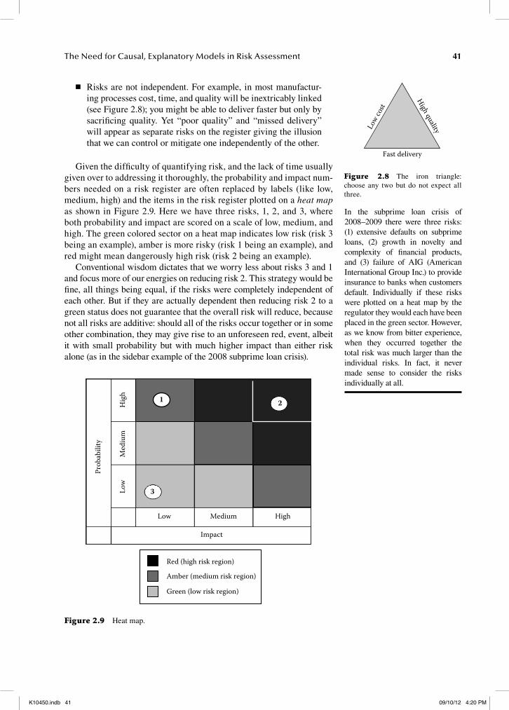
◾ Risks are not independent. For example, in most manufactur-ing processes cost, time, and quality will be inextricably linked (see Figure 2.8); you might be able to deliver faster but only by sacrificing quality. Yet “poor quality” and “missed delivery” will appear as separate risks on the register giving the illusion that we can control or mitigate one independently of the other.

Given the difficulty of quantifying risk, and the lack of time usually given over to addressing it thoroughly, the probability and impact num-bers needed on a risk register are often replaced by labels (like low, medium, high) and the items in the risk register plotted on a heat map as shown in Figure 2.9. Here we have three risks, 1, 2, and 3, where both probability and impact are scored on a scale of low, medium, and high. The green colored sector on a heat map indicates low risk (risk 3 being an example), amber is more risky (risk 1 being an example), and red might mean dangerously high risk (risk 2 being an example).

Conventional wisdom dictates that we worry less about risks 3 and 1 and focus more of our energies on reducing risk 2. This strategy would be fine, all things being equal, if the risks were completely independent of each other. But if they are actually dependent then reducing risk 2 to a green status does not guarantee that the overall risk will reduce, because not all risks are additive: should all of the risks occur together or in some other combination, they may give rise to an unforeseen red, event, albeit it with small probability but with much higher impact than either risk alone (as in the sidebar example of the 2008 subprime loan crisis).

In the subprime loan crisis of 2008–2009 there were three risks: (1) extensive defaults on subprime loans, (2) growth in novelty and complexity of financial products, and (3) failure of AIG (American International Group Inc.) to provide insurance to banks when customers default. Individually if these risks were plotted on a heat map by the regulator they would each have been placed in the green sector. However, as we know from bitter experience, when they occurred together the total risk was much larger than the individual risks. In fact, it never made sense to consider the risks individually at all.

Fast delivery

Low co

st

High quality

Figure 2.8 The iron triangle: choose any two but do not expect all three.

Hig

hLo

w

Low

Red (high risk region)

Amber (medium risk region)

Green (low risk region)

3

2

HighMedium

Impact

Med

ium

Prob

abili

ty

1

Figure 2.9 Heat map.

K10450.indb 41 09/10/12 4:20 PM


Risk is therefore a function of how closely connected events, systems, and actors in those systems might be. If you are a businessman the last thing you should do is look at the risks to your business separately using a risk register or heat map. Instead, you need to adopt a holistic outlook that embraces a causal view of interconnected events. Specifically:

To get rational measures of risk you need a causal model. Once you do this, measuring risk starts to make sense. It is much easier, though it requires an investment in time and thought.

2.5 Thinking about Risk Using Causal Analysis

It is possible to avoid all these problems and ambiguities surrounding the term risk by considering the causal context in which both risks and opportunities happen. The key thing is that a risk (and, similarly, an opportunity) is an event that can be characterized by a causal chain involving (at least):

◾ The event itself ◾ At least one consequence event that characterizes the impact

(so this will be something negative for a risk event and positive for an opportunity event)

◾ One or more trigger (i.e., initiating) events ◾ One or more control events that may stop the trigger event

from causing the risk event (for risk) or impediment events (for opportunity)

◾ One or more mitigating events that help avoid the consequence event (for risk) or impediment event (for opportunity)

This approach (which highlights the symmetry between risks and opportunities) is shown in the example of Figure 2.10.

Drivefast?

(helpsavoid riskevent)

(helps avoidnegativeconsequence)

Mitigant

Control

Speedwarnings?

Seatbelt?

Trigger

Risk event

Consequence

Crash?

Injury?

Drivefast?

(may stopopportunityevent)

(may stoppositiveconsequence)

Impediment

Impediment

Crash?

Nerves?

Trigger

Opportunityevent

Consequence

Makemeeting?

Wincontract?

(a) (b)

Figure 2.10 Causal taxonomy of risk/opportunity. (a) Causal view of risk. (b) Causal view of opportunity.

K10450.indb 42 09/10/12 4:20 PM


In practice, we would not gain the full benefits of building a causal model, unless we combine the risk events and opportunity events in a single model as in Figure 2.11.

In many situations it is actually possible to use completely neutral language (neither risk nor opportunity) as explained in the example of Box 2.4.

With this causal perspective of risk, a risk is therefore actually char-acterized not by a single event but by a set of events. These events each have a number of possible outcomes (to keep things as simple as pos-sible in the examples in this chapter we will assume each has just two outcomes: true and false). The uncertainty associated with a risk is not a separate notion (as assumed in the classic approach). Every event (and hence every object associated with risk) has uncertainty that is charac-terized by the event’s probability distribution (something we will cover in depth in Chapter 4).

Box 2.4 Using Neutral Language to Combine Risk/OpportunityCompanies undertake new projects because ultimately they feel the rewards outweigh the risks. As shown in Figure 2.12 the project delivery (whether it is late or not) and project quality are examples of key events associated with any new project. If the quality is bad or if the delivery is late then these represent risk events, whereas if the quality is good or the delivery is on time or even early, these represent opportunity events. The income is one of the conse-quence events of quality. It can be positive (in the event of a good quality project) or negative (in the event of a poor quality project). The company reputation is one of the consequences of both delivery and quality. It can be positive (if the quality is good and the delivery is on time) or negative (if either the quality is bad or the delivery is late).

Among the triggers, the risk/opportunity events have a common trigger, namely, key staff availability. If key staff become unavailable then the effect will be negative (risk), whereas if key staff are available then the effect will be positive (opportunity). The negative (positive) effect of key staff availability is controlled (impeded) by good (bad) staff incentives.

Among the mitigants/impediments there is a common factor, marketing. If the marketing is bad then even a good quality project delivered on time could lead to loss of reputation, whereas if it is good then even a poor quality project could lead to enhanced reputation.

Drivefast?

Speedwarnings?

Seatbelt?Crash?

Makemeeting?

Nerves?

Injury?

Wincontract?

Figure 2.11 Unified model with risk events and opportunity events.

K10450.indb 43 09/10/12 4:20 PM


Clearly risks in this sense depend on stakeholders and perspectives, but the benefit of this approach is that once a risk event is identified from a particular perspective, there will be little ambiguity about the concept and a clear causal structure that tells the full story. For example, consider the risk of Flood in Figure 2.13a. Because the risk event “Flood” takes the central role the perspective must be of somebody who has respon-sibility for both the associated control and mitigant. Hence, this is the perspective the local authority responsible for amenities in the village (rather than, for example, a householder in the village). A householder’s perspective of risk would be more like that shown in Figure 2.13b.

TriggersNew

requirements(many to few)

Project delivery(late to early)

Key Sta�availability

(bad to good)Managing

user expectations(bad to good)

Control/impediment Control/impedimentSta�

incentives(bad to good)

Sales sta�(bad to good)

Project quality(bad to good)

Marketing(bad to good)

Reputation(negative to

positive)

Income(negative to

positive)

Risk/opportunityevents

Mitigants/impediments

Consequences

Figure 2.12 Neutral causal taxonomy for risk/opportunity.

Dam burstsupstreamTrigger

Risk event

Consequence

Flood

Loss of life

Floodbarrier works

Rapid emergencyresponse

Control

Mitigant

Trigger

Risk event

Consequence

Flood

Loss of life

Sandbagsprotection

Adequateinsurance

House floods

Control

Mitigant

(a) (b)

Figure 2.13 Risk from different perspectives. (a) Flood risk from the local authority perspective. (b) Flood risk from the householder perspective.

K10450.indb 44 09/10/12 4:20 PM


What is intriguing is that the types of events are all completely inter-changeable depending on the perspective. Consider the example shown in Figure 2.14. The perspective here might be of the local authority lawyer. Note that:

◾ The risk event now is “Loss of life.” This was previously the consequence.

◾ “Flood” is no longer the risk event, but the trigger. ◾ “Rapid emergency response” becomes a control rather than a

mitigant.

It is not difficult to think of examples where controls and mitigants become risk events and triggers. This interchangeability stresses the symmetry and simplicity of the approach.

This ability to decompose a risk problem into chains of interrelated events and variables should make risk analysis more meaningful, prac-tical, and coherent. The causal approach can accommodate decision making as well as measures of utility but we make some simplifying assumptions to keep the material digestible:

◾ We model all variables as chance events rather than decision/actions that a participant might take.

◾ The payoffs for different decisions/actions are obvious and do not need to be assigned a utility value. So a “Law suit” or “Flood” is obviously a better outcome (of lower utility than “No law suit” or “No flood”) but we are not attempting here to mea-sure the utility in order to identify the optimum decision to take.

The Fallacy of Perfect Risk MitigationCauses of risk are viewed as uncer-tain, whereas mitigation actions to reduce impact are assumed to operate perfectly. This fallacy is widespread. Many risk management standards and guidelines assume that once a mitigation action is put in place that it will never degrade, be undermined, and hence will be invulnerable. Likewise, even sophis-ticated thinkers on risk can make the same mistake. For example, in his book The Black Swan, Taleb claims that high impact risk events cannot be readily foreseen and the only alternative answer is to mitigate or control the consequences of such risk events after the fact. How then do we guarantee perfect mitigation?

We take the view that the per-formance of mitigants is itself uncertain since they will need to be maintained and supported and if such maintenance and support is not forthcoming they will degrade.

Law suit

Trigger

Risk event

Consequence

Flood

Loss of life

Rapid emergencyresponse

Earlycompensation

offer

Control

Mitigant

Figure 2.14 Interchangeability of concepts depending on perspective.

K10450.indb 45 09/10/12 4:20 PM


2.6 Applying the Causal Framework to Armageddon

We already saw in Section 2.3.1 why the simple impact-based risk mea-sure was insufficient for risk analysis in the Armageddon scenario. In particular, we highlighted:

1. The difficulty of quantifying (in isolation) the probability of the meteor strike.

2. The difficulty of quantifying (in isolation) the impact of a strike.

3. The lack of meaning of a risk measure that is a product of (iso-lated measures of) probability and impact.

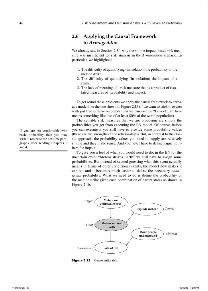
To get round these problems we apply the causal framework to arrive at a model like the one shown in Figure 2.15 (if we want to stick to events with just true or false outcomes then we can assume “Loss of life” here means something like loss of at least 80% of the world population).

The sensible risk measures that we are proposing are simply the probabilities you get from executing the BN model. Of course, before you can execute it you still have to provide some probability values (these are the strengths of the relationships). But, in contrast to the clas-sic approach, the probability values you need to supply are relatively simple and they make sense. And you never have to define vague num-bers for impact.

To give you a feel of what you would need to do, in the BN for the uncertain event “Meteor strikes Earth” we still have to assign some probabilities. But instead of second guessing what this event actually means in terms of other conditional events, the model now makes it explicit and it becomes much easier to define the necessary condi-tional probability. What we need to do is define the probability of the meteor strike given each combination of parent states as shown in Figure 2.16.

If you are not comfortable with basic probability then you may wish to return to the next few para-graphs after reading Chapters 3 and 4.

Control

Mitigant

Trigger

Event

Loss of life

Move peopleunderground

Explode meteor

Meteor oncollision course

Consequence

Meteor strikesEarth

Figure 2.15 Meteor strike risk.

K10450.indb 46 09/10/12 4:20 PM


There are some events in the BN for which we do need to assign unconditional probability values. These are represented by the nodes in the BN that have no parents; it makes sense to get unconditional proba-bilities for these because, by definition, they are not conditioned on any-thing (this is obviously a choice we make during our analysis). Such nodes can generally be only triggers, controls, or mitigants. An example, based on dialogue from the film, is shown in Figure 2.17.

The wonderful thing about BNs is that once you have supplied the initial probability values (which are called the priors) a Bayesian infer-ence engine (such as the one in AgenaRisk) will run the model and generate all the measures of risk that you need. For example, when you run the model using only the initial probabilities the model (as shown in Figure 2.18) computes the probability of the meteor striking Earth as

We are not suggesting that assign-ing the probability tables in a BN is always easy. You will generally require expert judgment or data to do it properly (this book will pro-vide a wealth of techniques to make the task as easy as possible). What is important is that it is easier than the classic alternative. At worse, when you have no data, purely subjective values can be supplied.

Meteor on collision courseExplode meteor

FalseFalse

FalseFalse

True

TrueTrue

True1.0 1.0 0.0 0.80.0 0.0 1.0 0.2

Figure 2.16 Conditional probability table for “Meteor strikes Earth.” For exam-ple, if the meteor is on a collision course then the probability of it striking the Earth is 1 if it is not destroyed, and 0.2 if it is. In completing such a table we no longer have to try to factor in any implicit conditioning events like the meteor trajectory.

FalseTrue

0.00100.999

Figure 2.17 Probability table for “Meteor on collision course with Earth.”

False

Trigger ControlMeteor on collision

Meteor strikes Earth

Explode meteor

True

0.1%

99.9%

False

True

0.899%

99.101%

False

True 1%

99%

Move peopleMitigant

Event

False

True 30%

70%

Loss of lifeConsequence

False

True 94.641%

5.359%

Figure 2.18 Initial risk of meteor strike.

K10450.indb 47 09/10/12 4:20 PM


99.1% and the probability of loss of life (meaning at least 80% of the world population) is about 94%.

In terms of the difference that Bruce Willis and his crew could make, we run two scenarios: one where the meteor is exploded and one where it is not. The results of both scenarios are shown in Figure 2.19.

Reading off the values for the probability of “Loss of life” being false we find that we jump from just over 4% (when the meteor is not exploded by Bruce) to 81% (when the meteor is exploded by Bruce). This massive increase in the chance of saving the world clearly explains why it mer-ited an attempt.

The main benefits of this approach are that

◾ Risk measurement is more meaningful in the context; the BN tells a story that makes sense. This is in stark contrast with the simple “risk equals probability times impact” approach where not one of the concepts has a clear unambiguous interpretation.

◾ Uncertainty is quantified and at any stage we can simply read off the current probability values associated with any event.

◾ It provides a visual and formal mechanism for recording and testing subjective probabilities. This is especially important for a risky event that you do not have much or any relevant data about (in the Armageddon example this was, after all, man-kind’s first mission to land on a meteorite).

False

Trigger ControlMeteor on collision

Meteor strikes Earth

Explode meteor

True

0.1%0.1%

99.9%99.9%

False

True

80.02%0.1%

19.98%99.9%

False

True

100%100%

Exploded: TrueNot Exploded: False

Move peopleMitigant

Event

False

True30%30%

70%70%

Loss of life

Consequence

False

True95.404%

19.081%

80.919%4.596%

Exploded=TrueExploded=False

Figure 2.19 The potential difference made by Bruce Willis and crew.

K10450.indb 48 09/10/12 4:20 PM


Although the approach does not explicitly provide an overall risk score and prioritization these can be grafted on in ways that are much more meaningful and rigorous. For example, we could

◾ Simply read off the probability values for each risk event given our current state of knowledge. This will rank the risks in order of probability of occurrence (this tells you which are most likely to happen given your state of knowledge of controls and triggers).

◾ Set the value of each risk event in turn to be fixed and read off the resulting probability values of appropriate consequence nodes. This will provide the probability of the consequence given that each individual risk definitively occurs. The risk prioritization can then be based on the probability values of consequence nodes.

Above all else the approach explains why Bruce Willis’s mission really was viable.

2.7 Summary

The aim of this chapter was to show that we can address some of the core limitations of the traditional statistical approaches using causal or explanatory models for risk assessment. Hopefully, the examples helped convince you that identifying, understanding, and quantifying the com-plex interrelationships underlying even seemingly simple situations can help us make sense of how risks emerge, are connected, and how we might represent our control and mitigation of them.

We have shown how the popular alternative approaches to risk mea-surement are, at worst, fundamentally flawed or, at least, limiting. By thinking about the hypothetical causal relations between events we can investigate alternative explanations, weigh the consequences of our actions, and identify unintended or (un)desirable side effects.

Of course it takes mental effort to make the problem tractable: care has to be taken to identify cause and effect, the states of variables need to be carefully defined, and probabilities need to be assigned that reflect our best knowledge. Likewise, the approach requires an analytical mindset to decompose the problem into classes of events and relationships that are granular enough to be meaningful but not too detailed that they are over-whelming. If we were omniscient we would have no need of probabili-ties; the fact that we are not gives rise to our need to model uncertainty at a level of detail that we can grasp, that is useful, and that is accurate enough for the purpose required. This is why causal modeling is as much an art (but an art based on insight and analysis) as a science.

Further ReadingAdams, J. (1995). Risk. Routledge.COSO (Committee of Sponsoring Organisations of the Treadway Commission).

(2004). Enterprise Risk Management: Integrated Framework, www.coso.org/publications.htm.

K10450.indb 49 09/10/12 4:20 PM


Fenton, N. E., and Neil, M. (2011). The use of Bayes and causal modelling in decision making, uncertainty and risk. UPGRADE, December 2011.

Hollnagel, E. (2009). The ETTO Principle: Efficiency-Thoroughness Trade-Off: Why Things That Go Right Sometimes Go Wrong. Ashgate.

Hubbard, D. W. (2009). The Failure of Risk Management: Why It’s Broken and How to Fix It, Wiley.

Sowell, T. (1987). A Conflict of Visions: Ideological Origins of Political Struggles. William Morrow.

K10450.indb 50 09/10/12 4:20 PM

The Need for Causal, Explanatory Models in Risk Assessment 2 The need for causa… · The Need for...

Documents

Transcript of The Need for Causal, Explanatory Models in Risk Assessment 2 The need for causa… · The Need for...