CHAPTER I1

THE NATURE OF EXPERIMENTAL

ERRORS IN REACTION KINETICS

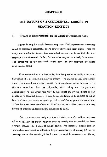
CHAPTER I1

THE NATURE OF EXPERIMENTAL ERRORS IN

REACTION KINETICS

1. Errors in Experimental Data: General Considerations.

Scientific enquiry would become very easy if all exper~mental quantities

could be measured accurately, say, to four or more significant digits There are

many uncontrollable factors that can d e c t measurements so that the true

response is not observed. In fact, the true value may never actually be observed

The deviations of the measured values from the true response are called

experimental errors.

If experimental error 1s inevitable, then the question naturally arlses as to

how much of it is tolerable in a given context The answer IS that, while errors

must be minimized to the extent possible, in circumstances where there can be no

(further) reduction, they are allowable, after ruling out c~~rnputat~onal

Irnproprletles, to the extent that they do not vitiate the system model or cast

doubts on ~ t s essential features. If they do so, the data must be rejected or put on

hold, and !he experimental des~gn improved or modlfied to permlt the acqu~s~tion

of data that meet these speclficatlons If, of course, the problem persists, one may

have to re-examme and redefine the system model ~tself.

One common reason why experimental data, even after refinement, may

refuse to fit into the model equation may be slmply that the model has been

wrongly chosen, i.e., a case of model failure. For instance, k~netic data on

intermediate concentration will refuse to give a satisfactory fit into eq. (5) for the

two-step, irreversible reaction, if the first step is reversible to some extent. Hence,

~t is of paramount importance that the system model must be exactly defined on

the basis of a close scrutiny of the data of a few prcliminq experiments,

examining especially for internal self-consistency, before designing and carrying

out a large number of them.

The distinguishing characteristics of systematic (or determinate) and

random (or indeterminate) errors are too elementary to warrant elaboration here

But certain features of these which are pertinent to reaction kinetics need be

restated to ensure that they are not overlooked under any circumstance.

The classical methods of kinetics, particularly of reactions in solution,

rested ma~nly on volumetric determinations, which are occasionally resorted to

even In modem times This necessitates the use of volumetric apparatus.

including flasks, pipettes and burettes, of balances and weights, and of chemicals

and solvents The need to calibrate carefully volumetr~c flasks, pipettes and

burettes, the last at every major graduation, by the standard procedures.

~ncorporating the buoyancy correction [16], cannot be overemphasized, for these

constitute a major source of systematic error that can be eliminated or adjusted

for Weights, particularly, fractional weights, of even A grade, have some errors,

ol[ui~ dcvclopiitg duc to wear and tcar; thcsc nccd pcr~odic calibration with NI'1.-

certified, standard weights, In order to eliminate an avoidable source of systematic

error If an electrical single-pan or an electron~c, top-loading balance is used, one

often becomes complacent ~n the bel~ef that one is employing a modem, rapid and

"accurate" instrument, and there l~es a frequent pitfall: these versat~le instruments

too require periodic recalibration of them scales, employing standard weights over

the11 entlre range, and the more sensitive an instrument is, the more prone it is to

be in error, particularly in the last decimal places of its readings As to chemicals,

one is sat~sfied to use them as such, especially if they are of a reputed brand and

of certified purity. There used to be a dictum in the classical days of the study of

reaction kinetics, that one should never take such certificates for granted: it was

mandatory to check its level of purity by analysis, before starting to use the

sample. This assay must be ustd to comct the concentration of a solution

prepared 'om a weight of the sample. Only the proper storage of a compound,

which is sensitive to air, moisture or light, can ensure the continued purity of an

assayed sample. Experimenters often carry out a perfunctory distillation of the

solvent, and use it days later; and, if the solvent is cenified to be of high purity by

the manufacturer, the inclination is to employ it as such without a d~stillat~on.

This practice can often introduce serious errors In the kinetic data, as many

organic solvents develop traces of peroxides which may promote unwanted side

react~ons

The classical methods of studying kinetics of chemical reactions, as already

noted, have shifted to the use of electronic instruments, particularly the

spectrophotometer. The advantages offered by the digital, self-recording, double-

beam, UV-visible spectrophotometer have been noted already: their availab~lity

places in the hands of the kineticist a versatile tool, capable of monitoring and

recording absorbance changes of a reaction mixture at five different wavelengths

at ~ntewals of a few seconds apart; just a few mL of the reaction mixture are

needed to study the course of the reaction, without his having to spend hours

distilling litres of the solvent, cleaning and drylng volumetric apparatus and

carrying out the kinetic run drawing aliquots of the reaction mixturc, perhaps one

every minute at the fastest, and determining the concentration of the reactant or

product in the frozenlquenched aliquot by titratlon using an ind~cator The cost of

the spectrophotometer seems worth, considering the speed ~t offers, its multt-

faceted h c t i o n s and, definitely, in terms of the time and labour saved. But it is

rarely remembered that the best of these instruments, such as those marketed by

Perk~n-Elmer or Hitachi, have a precision of i 0 002 Abs. (in terms of the

reproducibility of the readings) and an accuracy of just i 0.003 Abs. (in terms of

the absolute absorbance) in the range of 0 - 1.0 Abs. The accuracy is less than the

preclslon because the former includes systematic errors characteristic of the

indiv~dual instrument And the absolute absorbance can be guaranteed only ~f the

scale of the spbctrophotometer is calibrated over ~ t s entire range uslng carefully

prepared standard solutrons of potassium chromate in the visible reglon and of

potassium nitrate in the UV region 1171. The limitlng factor is the random

phenomenon of the Johnson shot-noise occurring in the photon counting device,

wh~ch cannot be completely eliminated even in the costliest versions [I 81.

One particular Instance of systematic error that often arises wlth

photometry and is usually ignored, is the failure of the solution to obey Bouguer-

Beer-Lambert's law, often known simply as Beer's law it is this law which

permits the use of absorbances in the place of concentrations In the system

equations. That the absorbance due to a given species at a fixed wavelength In a

cell of fixed path length varies in proportion to its concentration IS an assumption

of v~tal Importance to the use of the method. Fa~lures of the law in homogeneous

systems, i.e , solut~ons, are unknown 1191. The molecules act as absorpt~on

centres for radiat~on, and for the law to be val~d, they should act independently of

each other This restriction makes Beer's law to be a limiting law applicable to

solut~ons of concentrations less than 0.01M (of the absorb~ng species). At higher

concentrations, deviations from Beer's law occur due to the change In the

refractive index of the solution a- the concentration is changed. Bes~des,

interactions between different absorbing species, equilibria, associat~on and

dissociation can cause dev~ations from Beer's law If the deviations become

significant, very little can be done to salvage the sltuatlon

It IS essent~al that such systemalic errors be traced out 25 filr as poss~ble

and el~mlnated or adjusted for by appropriate steps In the experimental pruccdurc

or In the computations

Even when all systematic errors have been el~minated or adjusted for,

there remaln the indeterminate or random errors, wh~ch cannot be avolded

@together under any circumstance. These lead to the observed irreproduc~bll~ty

pf readings when the experiment is replicated, i.e., repeated under as far ident~cal

conditions as poss~ble. They are random in the sense that their direction and

magnitude can never be predicted. They cannot be controlled by the invest~gator

for any given experimental technique and arise when the measuring system or

lnsuument is worked at its most accurate limits. They arise as a result of a number

of unidentified or untraceable systematic errors, each of which makes a

conmbubon, whlch IS too small to be measured directly, but the11 cumulative

effect causes the replicate measurements to fluctuate randomly about the mean of

the set [20] The level of random error in an experiment, to be exactly defined in a

later sectlon, varies with the experimental procedure as well as w~th the

tn smen ta l method adopted. Thus, for example, the gravimetric methods of

estimatton of iron(11) are associated wlth smaller (random) errors than volumetric

methods; and. among various volumetric methods, titratlon w~th cerium(1V) 1s

more rel~able than titratlon w~th dichromate, uslng internal ind~cators. Th~s fact

permlts a worker to design experimental methods and choose procedures that

minimize the level of errors.

As experimental data invanably contaln errors, ~t is not possible to obtain

from them the true values of relevant parameters, such as rate coefficients, uslng

equations relating the data and the parameters. At best, only estimates of the

parameters can be calculated. The endeavour to obtain p&& estimates of the

parameters from experimental data, which contain errors, often depends on the

appltcation of correct statist~cal techniques

2. The Normal Distribution as the Law of Errors.

The term expertmental error, to the statistictan, connotes much more than

mere errors in both measurement and observation of a physical characteristic: it

cannot exclude the role of the experimenter himself and the errors of technique in

his performance of the experiment [21]: "In each particular situatton,

experimental error reflects (1) errors of experimentation, (2) errors of observation.

:3) errors of measurement, (4) the vanation of expertmental mater~al among

replications, i.e., repetitions of the same experiment, and (5) the comb~ned effect

of all extraneous factors that wuld influence the characteristics under study but

have not been singled out for attention in the current investigation."

In fact, the various ways of reducing the magnitude of experimental error

~nclude: (1) using more homogeneous experimental material or by careful

stratification of available material; (2) utilizing information provided by related

varlates. (3) using more care in conducting the experllncnt, and (4) as noted at the

end of the last section, using a more efficient expermental technique

While experimental data or observations may fall under any one of many

poss~ble distributions, such as the binomial, normal, Poisson, exponential, etc.

[21] (Ch 4), it was established by Gauss (1777-1855) that the random errors In

experimental measurement of most physical quantities have frequencies governed

by the normal distribution, which, stated simply, implies that smaller errors are

more likely than larger errors Though d~scovered by de Moivre in 1733 in

relation to the variation of some characteristic, such as heights or incomes of

~nd~viduals, which can vary continuously with no limit to the number of

ind~viduals w~ th d~rferent measurements [22], the normal d~st r~but~on 1s generally

associated with the namc of Gauss because of the latter's contributions to the

theory and methods of treatment of errors.

The normal distribution is determined by two parameters, the mean, p,

whlch locates the center of the distribution, and the standard deviation, G, which

measures the spread or variation of the ind~vidual measurements, in fact, a 1s the

scale, i.e., the unit of measurement, of the variable which is normally distributed.

It is described by the well-known bell-shaped curve. The formula for the ordinate

or height of the normal curve is

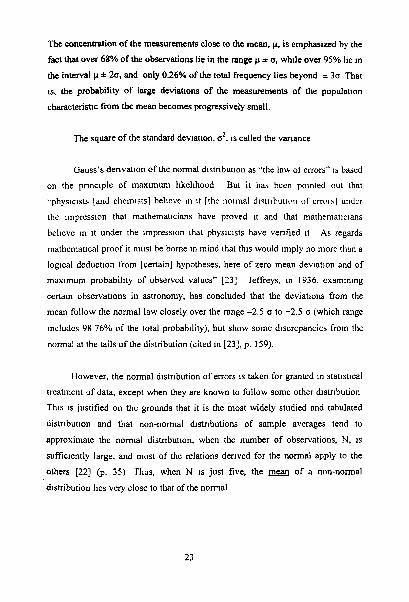
The concentration of the measurements close to the mean, p, is emphasized by the

fact that over 68% of the observations lie in the range p * a, whrle over 95% lie In

the interval p * 20, and only 0.26% of the total frequency lies beyond 3 0 That

IS, the probability of large deviations of the measurements of the populatron

characteristic from the mean becomes progressively small.

The square of the standard deviat~on, a', is called the variance

Gauss's derlvatron of the normal dlstrrbution as "the law ol errors" IS based

on the pnnc~ple of maximum likelihood But it has been polnted out that

"phys~cists [and chemlstsl hellcve In it jthc normal dlstrlhutlon of error\\ utidcr

the impression that mathematicians have proved 11 and that rnathematlcrans

believe In 11 under the impression that physlclsts have verified 11 As regards

mathematical proof it must be borne In mind that thrs would imply no more than a

logical deductron from [certain] hypotheses, here of zero mean deviation and of

maxlmum probability of observed values'' [23] Jeffreys, In 1936, examlnrng

cenaln observations in astronomy, has concluded that the deviations from the

mean follow the normal law closely over the range -2.5 o to +2.5 o (which range

~ncludcs 98 76% of the total probabrlity), but show some d~scrcpancics from the

normal at the tails of the distribution (cited in [23], p. 159).

However, the normal distr~bution of errors is taken for granted In stat~stlcal

treatment , ~ f data, except when they are known to follow some other distribution

This is justified on the grounds that it is the most widely studied and tabulated

distribution and that non-normal distr~butions of sample averages tend to

approximate the normal distnbution, when the number of observations, N, is

sufficiently large, and most of the relations derived for the normal apply to the

others 1221 (p. 35) Thus, when N is just five, the mean of a non-normal

drstribution 11es very close to that of the normal

Errors introduced during computations employing experimental data, such

as the crrors due to round-off or truncation. are of a different nature they follow

the uniform or rectangular distribution, In which every \aluc of the error has equal

probab~l~ty of occumng In the given range {a, b) Methods of deallng with such

non-normal errors, Including systematic errors that persist in the

measurementdobservations, are well-established [23] ( pp. 165-168). It 1s also

possible to accommodate unidentified systematic errors by treating them as

additional parameters to be determined by a regression technique [24]

It 1s the random, normal errors In the experimental data penainlng to

consccutlve reactions, the~r impact on the rel~abll~ty of the ratc coeffic~ents

calculated therefrom and the methods of arnvlng at better estimates of the rate

coeffic~ents, which are the main concerns of this thesis.

3. Representation of Error Levels.

If a constant or unchanging property, represented here by X, such as the

lel~gth of a plece of wire, the titre for the same volume of an a c ~ d solut~on w ~ t h a

standard base, the pH of a buffer solution, or the absorbance of a solution rn the

same cell at a given wavelength, 1s determined a number of tlmes, N, ~t will be

usually observed that these measurements or readings are all not den tical bul

differ slightly from one another in magnitude (which fact explains why the

constant quantity is here represented by X, a symbol usually reserved for

var~ables).

Assuming that all systematic errors have been el~mlnated (or adjusted for)

m d the differences are due solely to random errors inherent in all measurements,

hen, statistically, a @g estimate of the property is given by the population mean,

I, wh~le the population standard deviation, a, expresses the extent of imprecision

11 lrreproduc~bility of the measurement. These two quantities can be estimated

cxactly only whcn N -+ m, that IS, when the mcasurclncnt 1s ~cpcatcd .I g1c.11

many tlmes.

To obtaln good estrmates of the prec~sion of thc measurement of an)

characteristic, such as a tltre value or an absorbance rcadlng, 11 would rcqulre at

least thirty, preferably one hundred or more careful repetlttons of thc

~ncasurcment under idcntlcal experimental condlt~ons 1251. No aclcntlst liar thc

tune or patlence to pcrform such a large number of repl~cat~ons of an experiment

Most experiments are based on averages of SIX are less. The true mean and the

population standard deviatlon may never be known.

In real situat~ons, where the measurement is repeated only a few tlmes,

that IS, the slze of the sample (data) 1s small, one has to do w ~ t h the sample mean,

and the sample standard deviation, also known as the standard error In the

estlmate of X,

as the best estimates, respectively, of the true mean, p, and the true standard

deviatlon, a. The divisor R: - 1 ) appearing in eq (17) 1s important as ~t represents

the number of "degrees of freedom" and is equal to the number of independent

data used for calculating s, one having already been used for calculating the mean

I'hc variance, given by s2, is a measure of the prcclsron whlch IS unhlased by thc

sample size and has the desirable property of add~t lv~ty so that estlmales from

several sources of random error may be comb~ned, and it IS useful In probab~l~ty

calculations 1251.

Thus, if the titration of 10 mL of an a c ~ d solution with a standard alkal~

solution is repeated five times with a microburette, glving tltre values of 7 97,

8.02, 8.00, 7.99 and 8.02 mL, then the mean is 8.00 mL with a standard dev~at~on

of i 0.02(1) mL, a result usually expressed as 8.00 * 0.02 mL. The coefic~ent of

vanation, defined as 100(s/m), is then i 0.25%. often referred to as the

percentage error (in the estimate of the mean)

If the titratlon had been carried out with 5 mL aliquots, the mean tltre

m~ght be very close to 4.00 mL, but the standard deviation m~ght stdl be i 0 02

mL The error then becomes * 0.50%, ~f this set of titrat~ons alone IS considered

These apply when an invariant property is being estimated The tltrr values w ~ t h

both 5 and 10 mL aliquots here happen to have the same standard dev~at~on [or '1

constant vanance) Thls need not always be true In many cases. an ~nstrurnun~

exhiblts non-uniform variance at different points of its scale Thus, for e~amplc.

the Hitachi model U-2001 UV-visible spectrophotometer IS specified by the

manufacturer as having a photometric reproducibility of * 0.001 Abs In the

range 0 - 0 5 Abs., and of i 0 002 in the range 0.5-1 0 Abs

If the property being measured becomes a variant, as in the casc of the trtre

values obtained with aliquots drawn at d~fferent times from a rcactlon mlxture, or

In its photometric absorbance as the reaction progresses, the error level should be

defined relative to the hishest value observcd in the scrlc.; ofrcadinc\, hc 11 ;II thc

beginning, in the middle or towards the end of the experiment. In the parlance of

electrical (and electronic) instrumentation technology, the "nolse"(l e., the error)

level In a signal (reading) must be expressed relative to, I e., as a fractlon or

percentage of, the signal maximum (wherever ~t occurs), and not relatlve to the

local amplitude of that particular signal [26]. Again, un~form varlance of the

readings (signal amplitudes) is assumed.

The significance of this definition becomes apparent while cons~derlng the

following readings obtained in these laboratories by. Padma [27] In a particular

run in the oxidation of D-glucose with cerium(1V) in acid-sulphate medlum .

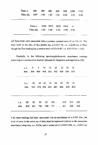
Time, s. 180 300 400 630 930 1290 1710

Titre,mL. 0.87 1.06 1.23 1 6 1 2.02 2 5 1 3 0 0

All these titres were associated with a constant standard error of i 0 01 m L The

error level in the data of thls kinetic run is 0.0115 56, i e.. 0 0018 (or 0 18%),

though the first reading has a relative error of 0.0110 87. I c , 0 01 15 (or 1 15°C)

Similarly, in the follow~ng spectromphotometric absorbance rcadlngs

pertaintng to a consecutive reaction obtained by Sargesson and reported In [2R]

t ,s . 0 5 10 15 20 25 30 35

Abs. ,844 884 908 ,923 ,932 938 ,936 ,933

t,s. 40 45 50 55 60 65 70 75

Abs. 925 .918 908 ,895 ,881 866 ,850 ,834

t ,s . 80 85 90 95 1 0 0 . . . 310 315 320

Abs. ,818 ,801 ,784 768 ,751 . .. ,411 ,408 ,406

~f all these readings had been associated with an uncertainty of 0.002 Abs , the

level of error in the entire set of data must be expressed relative to the rnaxlmum

absorbance observed, vlz., 0.938, and it works out to 0.00210.938, I e., 0.0021 (or

0.21%). Falure to grasp the sipficance of t h ~ s definition may lead to occas~onal.

gross misstatements of the error level of a serles of readings

Thus, if the absorbance of a reaction mixture changes steadily from 0 at

zero-time to 0.5 Abs. at the end of the reaction, and the readings taken In, say, a

Hitachi U-2001 spectrophotometer which has a reproducib~l~ty of i 0 001 Abs In

this region, the error works out to 100 x (* 0 001/0.5), i.e., i O 2% But, ~f the

absorbance increases from 0 to only 0.100 Abs, at the end, the error becomes

I00 x (*0.001/0.1), i.e., *1.0%, however, if the absorbance of the reactlon

mlxture is 0.400 Abs. at zero-times and increases by the same extent to 0 500

Abs. as the reaction ends, the standard error in the readings decreases to 100 x ( i

0.001/0.5), i.e.,0.2%.

In the rest of this thesis, the + sign associated with standard dev~at~ons 1s

dispensed with, but remains implied

1. W e i g h t i n g o f O b s e r v a t i o n s w h e n t h e y d i f f e r in Prec is ion .

When tllc obsc~vatlons of an cvolvlng system. such a\ thc rc;~dlilg ohta~iicd

durlng the course of a reactlon, are made w ~ t h d~fferent prec~s~ons (standard

errors), then stat~stlcally 11 makes no sense to asslgn the same or equal Importance

to all the readings obv~ously, the more preclse read~ngs have to be glven greater

Importance than the less preclse ones. This is done by attaching we~ghts to the

read~ngs commensurate with the11 preclslon.

An associated problem is the question of rejection of doubtful readings ~f

an observation has been repeated a number of times, and some of the readlngs

appears to deviate too much from rest, a s~rnple prescrlptlon is to reject those

readtngs wh~ch deviate by more than 2.5 (or, better, 3) standard dev~at~ons from

the mean of the rest of the readings, since there is, according to the normal

distribuhon, less than 1% chance that such d i n g s , known as 'outliers', are

consistent with the rest. (These are n f e m d to as 'black noise', as agalnst 'wh~te

noise', which deviate less, if the measurement has been made on an electr~cal or

electronic instrument). But when the number of replications is small, great cautlon

1s reqlured in adopting this devise. A simple Q test has been recommended for

rejection of outliers under such situations [20] @. 30-33). A detmled treatment of

outliers, including the various proposals of retaining anomalous readlngs by

we~ghting, is given in [29].

Weighting has been a vexatious problem in statlst~cs By dcfin~tlon, the

weights assigned are inversely proportional to the variances, i.e., to the squares of

the standard deviations, of the several observations [30],

where W,, IS the welght assigned to the nh reading, c: is ~ t s varlance and

CT~ = the varrance of unit weight, an arbitrary constant

If a serles of read~ngs taken In the course of an experiment 1s cons~dcred.

this necessarily irnpl~es that each reading in the series must be repl~cated, I e ,

determined a number of tunes, In order to know the standard dev~ation assoc~ated

w~ th it and asslgn the appropriate welght ([25], pp. 821-826), there 1s no polnt In

trylng to weight readlngs when the standard dev~at~on of each 1s unknown, as

happens when an experiment has been performed just once and each readlng In

the series of observations has been recorded only once Time constraints l nh~b~ t

any researcher from replicating all his experiments a number of tlrnes and ~t IS

generally considered sufficient if just a couple of expenments are run In

duplicates to ensure that the parameters, such as the rate coefficients, calculated

therefrom agree well to within certaln I~mits. Efforts to cany out more than

duplicates and to evaluate the standard deviations associated w th the different

read~ngs to enable the attachment of appropriate weights to & read~ng In the

serles, is seldom undertaken.

One way to overcome this lacuna 1s to tac~tly assume that all the read~ngs

In the experiment are all associated with the same Impreclslon, I e , standard error.

over the entlre range. This 1s a reasonable assumptlon lf the range covered IS not

very w~de and ~f the scale of the apparatus/rnstrument, I e , the burette or the

spectrophotometer, has been duly calibrated. Thus, the H~tachl model U-2001

UV-vls~ble spectrophotometer is specified by ~ t s manufacturer as havtng a

photometric reproducib~l~ty of i 0.001 Abs. In the range 0 - 0.5 Abs This can be

assumed to be constant over this range, though a particular instrument may havc

slightly d~ffering standard devrat~ons at different polnts of its scale w~thln th~s

range itself, a case of ~nstrumental idiosyncrasy.

With the assumption of uniform standard deviations (or variance), the

we~ghts to be assigned to all the readings in the range too become the same, and.

In fact, the weights can be discarded altogether

Throughout the present work, it is assumed that all rcad~ngs of an

experiment have the same, uniform variance While this situation may not obta~n

In practice when the readings extend to cover a wide range, the assumptlon does

greatly slmpllfy the calculations