The multiconfiguration time-dependent

Hartree (MCTDH) method: A highly efficient

algorithm for propagating wavepackets

M. H. Beck, A. Jackle, G. A. Worth, and H.-D. Meyer 1

Theoretische Chemie, Physikalisch-Chemisches Institut, Universitat Heidelberg,

Im Neuenheimer Feld 229, D-69120 Heidelberg, Germany

Abstract

A review is given on the multi-configuration time-dependent Hartree (MCTDH)method, which is an algorithm for propagating wavepackets. The formal derivation,numerical implementation, and performance of the method are detailed. As demon-strated by example applications, MCTDH may perform very efficiently, especiallywhen there are many (typically four to twelve, say) degrees of freedom. The largestsystem treated with MCTDH to date is the pyrazine molecule, where all 24 (!)vibrational modes were accounted for.

The particular representation of the MCTDH wavefunction requires special tech-niques for generating an initial wavepacket and for analysing the propagated wave-function. These techniques are discussed.

The full efficiency of the MCTDH method is only realised if the Hamiltonian canbe written as a sum of products of one-dimensional operators. The kinetic energy op-erator and many model potential functions already have this required structure. Forother potential functions, we describe an efficient algorithm for determining optimalfits of product form. An alternative to the product representation, the correlationdiscrete variable representation (CDVR) method, is also briefly discussed.

PACS: 31.15.Qg, 02.70.Ns

Keywords: MCTDH, multi-dimensional wavefunction propagation, quantum mo-

lecular dynamics

1 to whom correspondence should be sent(email: Hans-Dieter.Meyer@tc.pci.uni-heidelberg.de)

Preprint submitted to Elsevier 27 June 2012

Contents

1 Introduction 6

2 Time-dependent methods 9

2.1 Time-dependent versus time-independent methods 9

2.2 The standard propagation method 10

2.3 Time-dependent Hartree 11

2.4 Multi-configurational approaches 14

3 MCTDH: Theory 15

3.1 The MCTDH equations of motion 15

3.2 Choice of constraints 18

3.3 Density matrices and natural orbitals 21

3.4 Interaction picture 23

3.5 Non-adiabatic systems 24

4 MCTDH: Implementation 26

4.1 Representation of the single-particle functions 26

4.2 Product representation of the Hamiltonian 26

4.3 Time-dependent and Correlation DVR 28

4.4 Numerical scaling in brief 29

4.5 Mode combination 31

4.6 Effort of the single- and multi-set formulation 32

4.7 Complex absorbing potentials 33

4.8 Projector and density matrix 34

5 MCTDH: Integration schemes 36

5.1 The variable mean-field (VMF) integration scheme 36

5.2 The constant mean-field (CMF) integration scheme 36

6 Product representation of potential energy surfaces 48

6.1 Expansion in natural potentials 48

6.2 Contraction over one mode 50

2

6.3 Iterative optimisation 51

6.4 Separable weights 53

6.5 Error measures 54

6.6 Emulating non-separable weights 56

6.7 Concluding remarks 58

6.8 Applications 58

7 Preparation of the initial wavepacket 62

7.1 Generation of eigenstates by energy relaxation 62

7.2 Initial wavepacket correction schemes for scattering problems 63

8 Analysis 70

8.1 Matrix elements of operators 70

8.2 Difference between MCTDH wavefunctions 70

8.3 Auto-correlation function and photo-absorption spectra 72

8.4 Filter-diagonalisation and ro-vibrational spectra 74

8.5 State populations 75

8.6 Excitation and reaction probabilities computed by flux analysis 75

8.7 Run-time analysis of the accuracy of the propagation 82

9 Selected applications 86

9.1 Photo-dissociation of NOCl 86

9.2 Reactive scattering of H+D2 93

9.3 Surface scattering of N2/LiF(001) 99

9.4 Photo-excitation of pyrazine 102

10 Conclusions and outlook 109

Acknowledgements 111

A Variational principles for the time-dependent Schrodinger equation 112

B Discrete variable representation (DVR) 115

B.1 VBR and FBR representation of the potential 115

B.2 Diagonalisation DVR 117

3

B.3 Quadrature DVR 119

B.4 Examples 120

C The Lanczos and the Lanczos-Arnoldi integrator 129

D L2-error of the product representation 132

E Overview of software packages 135

E.1 The MCTDH program 135

E.2 The Potfit program 136

E.3 The Analyse programs 136

E.4 The Filter program 137

E.5 The MCTDH library 137

E.6 System requirements 137

References 139

4

List of Figures

1 Diagrammatic description of the CMF scheme 39

2 The CMF error in dependence of the error tolerance 41

3 H+D2(ν = 0, 1) reaction cross-sections 98

List of Tables

1 Errors of three product representations of collinear H+H2 60

2 Calculations to date using the MCTDH method 87

3 Computational resources for the photo-dissociation of NOCl 90

4 Computational resources for the 4-mode pyrazine model 105

5 Computational resources for the 9-mode pyrazine model 107

E.1 Platforms on which the MCTDH software has been installed 138

5

1 Introduction

During the last two decades the interest in quantum molecular dynamics hascontinuously risen [1–3]. Many new experiments, in particular those in thefield of femto-chemistry [4,5], require accompanying calculations for interpre-tation. A quantum mechanical study can be done in the time-independentpicture by diagonalisation of the Hamiltonian, or in the time-dependent pic-ture by propagation of a wavepacket. The standard method of solving theSchrodinger equation in either picture uses a representation of the wavepacketand Hamiltonian in an appropriate product basis. The method is thereby re-stricted by the computational resources required, which grow exponentiallywith the number of degrees of freedom.

As a result, for most of the above period numerically exact quantum me-chanical methods were in general restricted to tri-atomic systems. Due to theincrease in computer power and — equally important — the development ofnew efficient algorithms [6–10], the treatment of tetra-atomic systems is nowbecoming the state of the art, but studies of systems with more than six de-grees of freedom are in general still impossible. This limit has been pushedto larger dimensions by introducing special — and often problem specific —techniques, such as pre-diagonalisation of low-dimensional Hamiltonians (see[11–13] and references in the latter citation), or configuration selection byRayleigh-Schrodinger perturbation theory [14], or by wave operator methods[15].

The exponential scaling can be avoided by turning to more approximate, inparticular to semiclassical, methods. There have been new developments inthis field recently, showing impressive results [16]. We will discuss semiclassicalmethods no further and refer the reader to recent reviews [17,18].

In the time-dependent picture, on which we focus in the following, furtherapproximations have been developed which keep a fully quantum mechanicalpicture while removing the scaling problem in a more general manner. Thesemethods are exemplified by the TDH method (also known as time-dependentself-consistent field (TDSCF)) [19,20]. Here, the wavefunction is representedas a Hartree product of one-dimensional functions, resulting in a set of coupledone-dimensional equations of motion for the wavepacket (see Sec. 2.3). The ef-fort required is thus significantly reduced, but at the cost that the correlationbetween degrees of freedom is no longer correctly treated. Various schemeshave been developed to correct for this loss of correlation, e.g. by modify-ing the Hartree wavefunction by a time-dependent unitary operator [21–23],or by a multi-configurational (MC-TDSCF) approach, i.e. approximating thewavefunction by a number of Hartree products [24–26].

A particularly efficient variant of the MC-TDSCF approach is the multicon-figuration time-dependent Hartree (MCTDH) method [27–30]. The MCTDH

6

method, to which this review is devoted, combines the efficiency of a mean-fieldmethod, such as TDH, with the accuracy of a numerically exact solution. Usinga multi-configurational wavefunction ansatz, and solving the time-dependentSchrodinger equation by a variational method, leads to a set of coupled equa-tions of motion for the expansion coefficients and for the set of functions usedto build the Hartree product configurations. The latter are known as single-particle functions. As all possible configurations from the set of single-particlefunctions are build, the method is unfortunately also plagued by exponen-tial scaling. However, the base to be exponentiated is substantially smallercompared with the standard methods. This enables the treatment of largersystems by the MCTDH scheme.

In the limit of convergence with respect to the number of configurations, theresults of an MCTDH propagation are numerically exact. Even in this limitthe equations of motion, while seemingly complex, require less effort than thestandard method for large systems. An important feature of the method isthat, due to its variational character, a small set of single-particle functionscan be used to produce qualitatively good results with a minimum of effort.Internal checks using the population of the single-particle functions can thenbe used as a guide to the quality of the results.

The method has been applied successfully to a number of phenomena, suchas photodissociation [28,31–34] and photoabsorption spectra [35–38], predis-sociation [39], and reactive [40–46] and molecule-surface scattering [47–53].To demonstrate the applicability of the method to large systems, it should bementioned that converged calculations on a system with two coupled electronicstates and 24 nuclear degrees of freedom have been performed [36–38].

The purpose of this review is to provide an overview of the MCTDH theoryand the application of the method, with an emphasis on the description of thealgorithm (see Secs. 3 and 4). In App. E, a brief description of our MCTDHcomputer package is given.

A wavepacket propagation calculation can be divided into three parts:

(1) Generation of the initial wavepacket.(2) Propagation of the wavepacket.(3) Analysis of the propagated wavepacket.

These stages are described in detail.

The core of the MCTDH method is the wavepacket propagation. Here, oneimportant factor for the solution of the equations of motion is the choice of theprimitive basis used to represent the single-particle functions. In general a dis-crete variable representation (DVR) is used, and here various standard DVRsare described (see Appendix B): harmonic oscillator, Legendre, spherical har-monics, sine, and exponential, as well as the related fast Fourier transform

7

(FFT) basis. Various integration schemes are then possible. In particular, avery efficient integrator has been developed [54] which exploits the fact thatthe mean-field matrices, which correlate the motion of the single-particle func-tions, change slower in time than the single-particle functions themselves. Thisintegrator is described in Sec. 5.

The MCTDH propagation will in general be efficient only if the Hamiltonianis given in product form. The kinetic energy operator is usually in this form, asare many model potential operators, and profit has been made of this featurewhen investigating surface scattering [47–52] and vibronic coupling [35–37].When the potential does not have a product structure, one may either use therecently developed correlation DVR [55] (see Sec. 4.3), or fit the potential tothe desired form [56,57]. An algorithm accomplishing such a fit is discussed inSec. 6.

The initial form of the wavepacket must be chosen to fit the product form of theMCTDH wavefunction. A simple wavepacket may be chosen, and then mod-ified before propagation (see Sec. 7). For example, in many applications theinitial state is an eigenstate of a potential energy surface. These can be gener-ated by the method of energy relaxation (propagation in imaginary time). Forscattering problems, a Wentzel-Kramers-Brillouin (WKB) correction schemehas been developed that allows the initial wavepacket to be placed close tothe interaction region.

After the propagation has been completed, it is necessary to extract the quan-tities of interest. In this analysis step, which is addressed in Sec. 8, one againhas to take into account the particular form of the MCTDH wavefunction. Ex-amples are given for various evaluations: how to obtain a spectrum from theFourier transform of the autocorrelation function or by employing the filter-diagonalisation method, calculate the flux into a reaction channel, or monitorthe probability density along a coordinate.

Finally, in Sec. 9 examples of calculations are given to highlight the variouspoints of the algorithm, and to show how the possible choices affect the com-putational effort and accuracy of the calculation.

8

2 Time-dependent methods

In the earlier days of quantum molecular dynamics time-dependent methodswere largely ignored. Solving the time-independent Schrodinger equation wasconsidered as being significantly more efficient. This view began to changewhen Heller’s first paper on Gaussian wavepacket propagation [58] appearedin 1975. In the following years new numerical techniques were developed forsolving the time-dependent Schrodinger equation numerically exactly [7]. Inparticular, powerful integrators were invented [9], such as the split-operator[59–61], the Chebyshev [62], and the short iterative Lanczos [63] scheme. Sincethen the time-dependent approach has become popular.

2.1 Time-dependent versus time-independent methods

The quantal motion of the nuclei of a molecule or collision complex is mostnaturally described by solving the time-dependent Schrodinger equation. Ifthe Hamiltonian H is time-independent, however, the propagated wavepacketmay conveniently be expanded in the set of eigenstates of H (we use a unitsystem throughout where h = 1),

ψ(t) =∑

j

aj e−iEjtϕj , (1)

where

H ϕj = Ej ϕj and aj = 〈ϕj |ψ(0)〉 . (2)

This well-known expansion shows that the knowledge of a wavepacket ψ(t) forall times and the knowledge of all eigenstates ϕj and energies Ej are equivalent.The decision to follow the time-dependent or the time-independent approachis thus a matter of taste, and a question of numerical efficiency.

Although being formally equivalent, the time-independent approach seems tobe easier because one variable — the time — has disappeared from the equa-tions to be solved. However, in the time-independent picture one has to solvean eigenvalue problem, whereas using the time-dependent approach one isfaced with an initial value problem, which is mathematically simpler. Thispoint is of particular importance when treating scattering or half-collision(e.g. photo-dissociation) processes. In these cases the eigenstates become con-tinuum functions with complicated scattering boundary conditions. The sumin Eq. (1) has to be replaced by an integral over the continuum states. In thetime-dependent framework, on the other hand, the wavepacket remains square

9

integrable, and there is essentially no difference in propagating a wavepacketthat is a superposition of bound or continuum states.

The time-dependent picture becomes even more attractive when turning toapproximate methods. One may distinguish two classes of approximations.Methods from the first class simplify the Hamiltonian. The coupled statesapproximation [64,65] (also known as jz-conserving approximation) is a typicalexample out of this category. Approximations of this type can be employed inboth the time-independent and time-dependent framework. In both picturesthey introduce the same errors and lead to a similar reduction of the numericaleffort.

The other class is based on approximating the wavefunction. Here a typi-cal example is the Hartree approximation, which writes the multi-dimensionalwavefunction as a simple product of one-dimensional functions. This approachworks in general much better in the time-dependent picture, because a time-dependent wavepacket is usually more or less localised (in phase space), whilean eigenstate is typically rather delocalised. Hence the time-dependent ap-proach enables the use of approximations which are more efficient and moreaccurate than their time-independent counterparts.

Besides these technical advantages, a time-dependent description often leadsto a better understanding of the physical process under discussion. Finally, ifthe Hamiltonian is itself time-dependent, one must of course adopt the time-dependent picture.

2.2 The standard propagation method

The standard approach for solving the time-dependent Schrodinger equationis the numerically exact propagation of a wavepacket represented in a time-independent product basis set, i.e. the wavefunction is written as

Ψ(Q1, . . . , Qf , t) =N1∑

j1=1

. . .Nf∑

jf=1

Cj1...jf (t)f∏

κ=1

χ(κ)jκ (Qκ) , (3)

where f specifies the number of degrees of freedom, Q1, . . . , Qf are the nuclearcoordinates, the Cj1...jf denote the time-dependent expansion coefficients, and

the χ(κ)jκ are the time-independent basis functions for degree of freedom κ. To

allow an efficient and accurate evaluation of the action of the Hamiltonian Hon the wavefunction Ψ, one usually chooses the Nκ basis functions χ

(κ)jκ to be

the DVR/FBR functions of a collocation method, typified by those discussedin App. B.

10

The equations of motion for Cj1...jf (t) can be derived from the Dirac-Frenkelvariational principle [19,66]

〈δΨ |H − i∂t |Ψ〉 = 0 , (4)

where ∂t denotes the partial derivative with respect to time, leading to

iCJ =∑

L

HJLCL , (5)

where we have established the multi-index J = j1 . . . jf (and analogously

for L). HJL = 〈χ(1)j1 . . . χ

(f)jf| H | χ(1)

l1. . . χ

(f)lf〉 is the matrix representation of

the Hamiltonian given in the product basis set χ(κ)jκ . Equation (5) forms a

system of coupled linear first-order ordinary differential equations, which canbe solved by integrators explicitly designed for equations of that kind [9], suchas the split-operator [59–61], Chebyshev [62] or Lanczos [63] methods.

The computational effort of this numerically exact treatment grows exponen-tially with the number of degrees of freedom f . To see this we define the effortas the number of floating point operations to be carried out, and assume forsimplicity that the same number N = N1 = . . . = Nf of basis functions isemployed for each degree of freedom. If one utilises the fact that the kineticenergy part of H can be written in tensor form and that the potential energyis diagonal on a DVR grid, the computational effort necessary to evaluatethe right hand side of Eq. (5) is then proportional to fN f+1. Here we haveneglected the effort for computing the matrix representation of H since thishas to be done only once at the beginning of the propagation. This scalingbehaviour generally restricts the standard method to systems with not morethan five or six degrees of freedom.

2.3 Time-dependent Hartree

In order to circumvent the disadvantageous scaling behaviour of a numeri-cally exact propagation, approximate methods for solving the time-dependentSchrodinger equation have been developed. The most widely used approximatescheme is the time-dependent Hartree (TDH) method [19,20] (also knownas the time-dependent self-consistent field (TDSCF) method), which we willbriefly discuss in the following. Understanding this approach will pave the wayto understanding the MCTDH method. To keep the discussion as simple aspossible we restrict ourselves to the treatment of two degrees of freedom only.The extension to larger systems is straightforward.

11

In the TDH approximation the wavefunction is written as

Ψ(x, y, t) = a(t)ϕ1(x, t)ϕ2(y, t) , (6)

where a is a time-dependent complex number and ϕ1 and ϕ2 are known assingle-particle functions or orbitals. The product ϕ1ϕ2 is called a Hartree prod-uct.

Equation (6) does not determine the single-particle functions uniquely, sincephase and normalisation factors may be shifted from ϕ1 to ϕ2 or even to a.The introduction of the (redundant) term a(t) allows us to freely choose thephases of both ϕ1 and ϕ2. We write the constraints that fix the phases indifferential form:

〈ϕ1 | ϕ1〉 = 〈ϕ2 | ϕ2〉 = 0 . (7)

These constraints also guarantee that the norm of ϕ1 and ϕ2 does not change.Hence ϕ1 and ϕ2 will stay normalised throughout the propagation,

‖ϕ1(t)‖= ‖ϕ2(t)‖= 1 , (8)

if they are normalised initially.

The equations of motion for a(t), ϕ1(t), and ϕ2(t) are derived from the Dirac-Frenkel variational principle (4). Variation with respect to a yields

〈ϕ1ϕ2 | iaϕ1ϕ2 + iaϕ1ϕ2 + iaϕ1ϕ2 −Haϕ1ϕ2〉 = 0 (9)

or, with the aid of the constraints (7) and (8),

ia = 〈H〉a , (10)

where 〈H〉 = 〈ϕ1ϕ2 |H | ϕ1ϕ2〉. Similarly, by varying ϕ1 and ϕ2 we obtain

iϕ1 =(H(1) − 〈H〉

)ϕ1 and iϕ2 =

(H(2) − 〈H〉

)ϕ2 , (11)

with the mean-field operators

H(1) = 〈ϕ2 |H | ϕ2〉 and H(2) = 〈ϕ1 |H |ϕ1〉 . (12)

Equation (11) can be alternatively written as

iϕ1 =(1− |ϕ1〉〈ϕ1 |

)H(1)ϕ1 and iϕ2 =

(1− |ϕ2〉〈ϕ2 |

)H(2)ϕ2 , (13)

12

where | ϕ1〉〈ϕ1 | and | ϕ2〉〈ϕ2 | denote the projectors onto the state ϕ1 orϕ2, respectively. It is now obvious that the equations of motion satisfy theconstraints (7) and (8).

The TDH wavefunction can be considered as being propagated by an effectiveHamiltonian Heff ,

iΨ = Heff Ψ , (14)

with

Heff = H(1) +H(2) − 〈H〉 . (15)

To investigate the errors introduced by the TDH approximation let us assumethat the Hamiltonian has the form

H = − 1

2m1

∂2

∂x2− 1

2m2

∂2

∂y2+ V1(x) + V2(y) +W1(x)W2(y) . (16)

In this case one finds that

Heff = H −(W1 − 〈W1〉

)(W2 − 〈W2〉

), (17)

or

iΨ−HΨ = −(W1 − 〈W1〉

)(W2 − 〈W2〉

)Ψ . (18)

The right hand side of the above equation describes the error introduced bythe Hartree approximation. The error vanishes if the Hamiltonian is separable,and it becomes small if the functions W1 and W2 are almost constant over thewidth of the single-particle functions ϕ1 and ϕ2, respectively. This is whythe time-dependent Hartree method is usually more accurate than the time-independent Hartree method; the time-dependent wavepacket is likely to belocalised, whereas the eigenstates are usually very delocalised.

The TDH approximation has been intensively used by Gerber and coworkers[67–70] who have applied it to systems with very many (≈ 100) modes. Thetreatment of such large systems became possible through the development ofthe classical based separable potential (CSP) method [67], which is a veryefficient way to approximately evaluate the mean-fields. Although the use ofthe CSP method destroys the variational basis of the TDH approach, it seemsto introduce only small errors.

13

2.4 Multi-configurational approaches

As the performance of the TDH method is often rather poor, an obvioussuggestion is to improve the method by taking several configurations into ac-count. The first investigations on multi-configurational time-dependent SCF(MC-TDSCF) — as the method was called — were made by Makri and Miller[24] and by Kosloff et al. [25], both in 1987. These important early investi-gations were formulated for two degrees of freedom and two configurationsonly. As the two-dimensional case is a special case, generalisation of these ap-proaches is not obvious. The latter approach has been developed further [26],but not pursued later.

In this review we will discuss the multiconfiguration time-dependent Hartree(MCTDH) method. This algorithm, which was published in 1990 [27], is fullygeneral from its outset. The number of degrees of freedom and the number ofsingle-particle functions per degree of freedom is arbitrary. The latter featureallows MCTDH to cover the full range of quality of approximation, from TDHto numerically exact. The particular choice of constraints used in the deriva-tion of MCTDH (see Eq. (22) below) makes the working equations — albeitseemingly complex — simpler than those of their predecessors.

It should be noted that the acronym MC-TDSCF is used for the whole familyof multi-configurational approaches, while MCTDH, being uniquely defined inSec. 3.1, is a special variant of the MC-TDSCF family.

Because of the complexity of MCTDH, simplified methods have been tried.One may for instance perform a TDH calculation, diagonalise the mean-fieldsto obtain a full set of single-particle functions, and generate a correlated wave-packet via a time-dependent CI in a space of single-particle functions. Thisapproach — called TDH-CI [71–75], or TDSCF with CI corrections [76,77] —may be regarded as an approximation to MCTDH. The single-particle func-tions are obtained here in a simplified way. However, it is not important tosimplify the equations of motion of the single-particle functions, because theirsolution requires only a small fraction of the total effort when larger systemsare considered. But it is of crucial importance to have optimal single-particlefunctions in order to keep the number of configurations as small as possible.Being fully based on an variational principle, as is detailed in the followingsection, the MCTDH working equations generate optimal single-particle func-tions.

14

3 MCTDH: Theory

In this section the working equations of the MCTDH scheme [27–30] are de-rived. The MCTDH scheme is motivated by the discussion of the precedingsections 2.2 and 2.3, since MCTDH combines the benefits of the standard,numerically exact, wavefunction propagation and the time-dependent Hartreeapproaches. We also describe several modifications of the original MCTDHalgorithm that serve to further improve the efficiency and extend the applica-bility of the method.

3.1 The MCTDH equations of motion

In the MCTDH scheme the TDH approach is generalised by writing the wave-function Ψ, which describes the molecular dynamics of a system with f degreesof freedom, as a linear combination of Hartree products, i.e. the ansatz for thewavefunction becomes

Ψ(Q1, . . . , Qf , t) =n1∑

j1=1

. . .nf∑

jf=1

Aj1...jf (t)f∏

κ=1

ϕ(κ)jκ (Qκ, t) , (19)

where Q1, . . . , Qf are the nuclear coordinates, the Aj1...jf denote the MCTDH

expansion coefficients, and the ϕ(κ)jκ are the nκ expansion functions for each

degree of freedom κ, known as single-particle functions. Setting n1 = . . . =nf = 1 one arrives at the TDH wavefunction. TDH is thus contained in MC-TDH as a limiting case. As the numbers nκ are increased, the more accuratethe propagation of the wavefunction becomes, and the MCTDH wavefunctionmonotonically converges towards the numerically exact one, Eq. (3), as nκ

approaches Nκ. The computational labour, however, increases strongly withincreasing values of nκ. We will later provide some guidelines as to how tochoose the numerical values of the nκ consistently, in order to achieve somedesired level of accuracy (see Sec. 8.7). Here we note that the nκ should obey[27]

n2κ ≤

f∏

κ′=1

nκ′ , (20)

otherwise there will be redundant configurations. For two dimensions the con-dition n1 = n2 follows, but for higher dimensions Eq. (20) usually does notpose a constraint.

As in the case of the TDH approximation, the MCTDH wavefunction rep-resentation (19) is not unique, one may linearly transform the single-particle

15

functions and the expansion coefficients while still representing the same wave-function. These redundancies prohibit singularity-free well-defined equationsof motion. Uniquely defined propagation is obtained by imposing the con-straints

〈ϕ(κ)j (0) |ϕ(κ)

l (0)〉 = δjl (21)

and

〈ϕ(κ)j (t) | ϕ(κ)

l (t)〉 = −i 〈ϕ(κ)j (t) |g(κ) |ϕ(κ)

l (t)〉 (22)

on the single-particle functions. Here the constraint operator g(κ) is a Hermi-tian, but otherwise arbitrary, operator acting exclusively on the κth degree offreedom. The constraints (21) and (22) imply that the initially orthonormalsingle-particle functions remain orthonormal for all times.

Before presenting the MCTDH working equations we simplify the notation byestablishing the composite index J and the configurations ΦJ :

AJ = Aj1...jf and ΦJ =f∏

κ=1

ϕ(κ)jκ . (23)

We also introduce the projector on the space spanned by the single-particlefunctions for the κth degree of freedom:

P (κ) =nκ∑

j=1

|ϕ(κ)j 〉〈ϕ(κ)

j | . (24)

The single-hole functions Ψ(κ)l are defined as the linear combination of Hartree

products of (f − 1) single-particle functions that do not contain the single-particle functions for the coordinate Qκ,

Ψ(κ)l =

∑

j1

. . .∑

jκ−1

∑

jκ+1

. . .∑

jf

Aj1...jκ−1ljκ+1...jfϕ(1)j1 . . . ϕ

(κ−1)jκ−1

ϕ(κ+1)jκ+1

. . . ϕ(f)jf

=∑

J

κAJκ

lϕ(1)j1 . . . ϕ

(κ−1)jκ−1

ϕ(κ+1)jκ+1

. . . ϕ(f)jf, (25)

where in the last line Jκl denotes a composite index J with the κth entry set

at l, and∑κ

J is the sum over the indices for all degrees of freedom excludingthe κth.

The single-hole functions enable us to define the mean-fields

〈H〉(κ)jl = 〈Ψ(κ)j |H |Ψ(κ)

l 〉 (26)

16

and density matrices

ρ(κ)jl = 〈Ψ(κ)

j |Ψ(κ)l 〉

=∑

j1

. . .∑

jκ−1

∑

jκ+1

. . .∑

jf

A∗j1...jκ−1jjκ+1...jf

Aj1...jκ−1ljκ+1...jf (27)

=∑

J

κA∗

JκjAJκ

l.

In Sec. 3.3 a discussion on the density matrix is given. Note that 〈H〉(κ)jl is an

operator acting on the κth degree of freedom, and that the trace of ρ(κ) equals‖ Ψ ‖2 due to the orthonormality of the single-particle functions.

Using the notation introduced above, we may express Ψ, Ψ, and the variationδΨ as

Ψ=∑

J

AJΦJ =nκ∑

j=1

ϕ(κ)j Ψ

(κ)j , (28)

Ψ=f∑

κ=1

nκ∑

j=1

ϕ(κ)j Ψ

(κ)j +

∑

J

AJΦJ , (29)

δΨ

δAJ

=ΦJ andδΨ

δϕ(κ)j

= Ψ(κ)j . (30)

With the aid of the variational principle (4) (see also App. A) and the con-straints (21) and (22) one finds when varying the coefficients:

〈ΦJ |H |Ψ〉 − i〈ΦJ |Ψ〉 = 0 (31)

and hence

iAJ = 〈ΦJ |H |Ψ〉 −f∑

κ=1

nκ∑

l=1

g(κ)jκlAJκ

l, (32)

where g(κ)jl = 〈ϕ(κ)

j |g(κ) |ϕ(κ)l 〉.

Varying with respect to the single-particle functions yields

〈Ψ(κ)j |H |Ψ〉 = i〈Ψ(κ)

j |f∑

κ′=1

nκ′∑

l=1

ϕ(κ′)l Ψ

(κ′)l 〉+ i

∑

J

〈Ψ(κ)j |ΦJ〉AJ . (33)

From this one obtains

17

inκ∑

l=1

ρ(κ)jl ϕ

(κ)l = 〈Ψ(κ)

j |H |Ψ〉 −∑

J

〈Ψ(κ)j |ΦJ〉 〈ΦJ |H |Ψ〉

+nκ∑

k,l=1

ρ(κ)jk g

(κ)lk ϕ

(κ)l . (34)

Noticing that

∑

J

〈Ψ(κ)j |ΦJ〉 〈ΦJ | = P (κ)〈Ψ(κ)

j | (35)

and

〈Ψ(κ)j |H |Ψ〉 =

nκ∑

l=1

〈H〉(κ)jl ϕ(κ)l , (36)

and after some rearrangement, one finally arrives at the MCTDH workingequations

iAJ =∑

L

〈ΦJ |H |ΦL〉AL −f∑

κ=1

nκ∑

l=1

g(κ)jκlAJκ

l, (37)

iϕ(κ)= g(κ)1nκϕ(κ) +

(1− P (κ)

) [(ρ(κ)

)−1〈H〉(κ) − g(κ)1nκ

]ϕ(κ) , (38)

where a vector notation has been adopted for the single-particle functions with

ϕ(κ) =(ϕ(κ)1 , . . . , ϕ(κ)

nκ

)T, (39)

ρ(κ) the density matrix, 〈H〉(κ) the matrix of mean field operators, and 1nκ

the nκ × nκ unit matrix. The choice of the constraint operator, g(κ), can thenbe used to change the final form of the equations of motion, either to simplifythem, or to highlight different aspects of the dynamics. This problem will beaddressed in detail in Sec. 3.2.

We close this section by emphasising that the MCTDH equations conserve thenorm and, for time-independent Hamiltonians, the total energy. This followsdirectly from the variational principle (cf. App. A).

3.2 Choice of constraints

In the previous section 3.1, the MCTDH equations of motion were derivedwithout explicitly defining the constraint single-particle operator, g(κ). Thechoice of this operator is arbitrary, and it does not affect the quality of the

18

MCTDH wavefunction. It does however affect the numerical performance ofthe integration of the equations of motion, as it is possible to transfer the workfrom the integration of the equations of motion for the coefficients to thosefor the single-particle functions. Here we describe some of the possible choicesfor this constraint operator.

The simplest choice is to set g(κ) = 0 for all degrees of freedom. When this isdone, the MCTDH equations of motion read

iAJ =∑

L

〈ΦJ |H |ΦL〉AL , (40)

iϕ(κ)=(1− P (κ)

) (ρ(κ)

)−1〈H〉(κ)ϕ(κ) . (41)

The relationship to the standard method equations of motion, Eq. (5), is hereclear. When nκ = Nκ the single-particle function basis is complete, and so theright-hand side of Eq. (41) is zero, resulting in a time-independent basis.

A second possibility is to use the fact that the Hamiltonian may contain certainterms that operate only on one degree of freedom. Denoting these separableterms by h(κ) the Hamiltonian can then be written

H =f∑

κ=1

h(κ) +HR , (42)

where the residual part, HR, includes all the correlations between the degreesof freedom. If the constraints g(κ) = h(κ) are now taken, the MCTDH equationsof motion change to

iAJ =∑

L

〈ΦJ |HR |ΦL〉AL , (43)

iϕ(κ)=[h(κ)1nκ

+(1− P (κ)

) (ρ(κ)

)−1〈HR〉(κ)]ϕ(κ) , (44)

where the matrix elements 〈ΦJ | HR | ΦL〉 and mean-fields 〈HR〉(κ)jl are nowevaluated using only the residual part of the Hamiltonian.

Compared to Eq. (43), the working equation (40) has the disadvantage thatthe full Hamiltonian H instead of the residual Hamiltonian HR is employed inthe propagation of the MCTDH coefficients, which is computationally moreexpensive. While it seems that Eq. (44) also gains over the working equation(41) by using only the residual Hamiltonian to build the mean fields, in practicethis is not the case, as Eq. (41) can be rewritten to also take advantage of theseparable parts of the Hamiltonian:

iϕ(κ) =(1− P (κ)

) [h(κ)1nκ

+(ρ(κ)

)−1〈HR〉(κ)]ϕ(κ) . (45)

19

In many cases the different amount of work required to propagate the MCTDHcoefficients can make a noticeable difference to the required computer time.For example, in the case of the 4-mode model for the photo-excitation of thepyrazine molecule [35], a calculation employing Eqs. (40) and (45) is 8% slowercompared with one using Eqs. (43) and (44).

The use of Eq. (41) or (45) however implies that the motion of the single-particle functions is minimised, because the projector exclusively allows mo-tions in directions perpendicular to the space spanned by the single-particlefunctions. Reducing the motion of the single-particle functions to a minimummay be favourable for some integrators. This is for example the case whenusing the constant-mean-field integrator described below in Sec. 5.2, whichhas been developed to optimally integrate the MCTDH equations of motion.

It is important to note that these two sets of equations are connected by asimilarity transformation:

ϕ(κ)j =

∑

l

ϕ(κ)l U

(κ)lj , (46)

Aj1...jf =∑

l1

. . .∑

lf

(U (1)†

)j1l1. . .(U (f)†

)jf lf

Al1...lf , (47)

where, if A and ϕ are the coefficients and single-particle functions from Eqs.(40) and (41), and A and ϕ are those from Eqs. (43) and (44), then U (κ) =

exp(ih(κ)t), with h(κ)jl = 〈ϕ(κ)

j |h(κ) |ϕ(κ)l 〉. Similar transformations connect the

basis functions propagated using any two constraint operators, replacing h(κ)

in the unitary transformation operator with the difference between the con-straint operators. This underlines the fact the constraints make no differenceto the accuracy of the representation of the wavefunction.

One last possibility for the choice of constraints will be mentioned here. AHermitian operator can be chosen that is completely described within thesingle-particle basis, i.e.

g(κ) =nκ∑

l,j=1

|ϕ(κ)l 〉 g

(κ)lj 〈ϕ

(κ)j | . (48)

The constraint operator to the right of the projector in Eq. (38) then disap-pears, and the equations of motion read

iAJ =∑

L

〈ΦJ |H |ΦL〉AL −f∑

κ=1

nκ∑

l=1

g(κ)jκlAJκ

l, (49)

iϕ(κ)=(g(κ)

)Tϕ(κ) +

(1− P (κ)

) (ρ(κ)

)−1〈H〉(κ)ϕ(κ) , (50)

20

where g(κ) is the constraint operator matrix with elements g(κ)lj (see Eq. (48)).

(Eq. (50) holds generally, as it may be derived directly from Eq. (34)). Itis of course also possible to add the separable Hamiltonian terms to theseconstraints, replacing H by HR, and replacing g(κ)

T

by h(κ)1nκ+ g(κ)

T

.

Constraint operators of this type are time-dependent, and the matrix repre-sentation must be recalculated at each step. They may be used to enforce thesingle-particle functions to retain a particular property. An example is givenbelow in Sec. 3.3, where constraints of this form are developed so that thesingle-particle functions are the natural orbitals of the system, i.e. the densitymatrices remain diagonal.

3.3 Density matrices and natural orbitals

So far we have said nothing about the physical meaning of the density matrixρ(κ) defined in Eq. (27). For an interpretation of ρ(κ) we turn to the relateddensity operator. Using the definitions (25) and (27) we express the densityoperator as

ρ(κ)(Qκ, Q′κ)=

nκ∑

j,l=1

ϕ(κ)j (Qκ) ρ

(κ)lj ϕ

(κ)∗

l (Q′κ) (51)

=∫Ψ∗(Q1, . . . , Q

′κ, . . . , Qf )Ψ(Q1, . . . , Qκ, . . . , Qf )

× dQ1 . . . dQκ−1 dQκ+1 . . . dQf .

This shows that ρ(κ) is similar to the well-known one-particle density of elec-tronic structure theory [78], and related to a reduced density matrix [79]. (Notethat our density matrix is the transposed of the matrix representation of thedensity operator in the set of the single-particle functions.) Diagonalising theoperator ρ(κ) yields the natural populations and natural orbitals [27,28,47,80],defined as the eigenvalues and eigenvectors of ρ(κ). Since we are dealing withdistinguishable particles we have a separate density matrix for each degree offreedom.

In contrast to the single-particle functions, the natural orbitals are uniquelydefined. The former depend on the choice of the single-particle constraint op-erators g(κ) (see Sec. 3.2), as well as on the chosen set of initial single-particlefunctions. Replacing the single-particle functions of ansatz (19) by the natu-ral orbitals we arrive at a unique MCTDH representation of the wavefunction.Furthermore, the natural populations characterise the contribution of the re-lated natural orbitals to the representation of the wavefunction. Small naturalpopulations indicate that the MCTDH expansion converges, and this providesan important internal check on the quality of the computed solution. (See for

21

instance Refs. [28,31,34,39,40,47,50–52] for examples.) For very small or evenvanishing eigenvalues, the Hermitian and positive semi-definite density matrixwill become singular. This numerical problem is addressed in Sec. 4.8.

As mentioned above in Sec. 3.2, it is possible to define a set of constraintoperators, g(κ), using Eq. (48) such that the single-particle functions retainthe “natural” form, i.e. the density matrices remain diagonal during the prop-agation [80]. Using Eqs. (25), (27), (28), and (37) one may write the time-derivative of the density matrix as

iρ(κ)jl = 〈Ψ(κ)

j ϕ(κ)l |H |Ψ〉 − 〈Ψ |H |Ψ

(κ)l ϕ

(κ)j 〉

−nκ∑

k=1

(ρ(κ)jk g

(κ)lk − ρ

(κ)kl g

(κ)kj

)(52)

+f∑

κ′ 6=κ

(〈Ψ |g(κ′) |Ψ(κ)

l ϕ(κ)j 〉 − 〈Ψ(κ)

j ϕ(κ)l |g(κ

′) |Ψ〉),

where g(κ)lk is as before the matrix representation of the constraint operator in

the single-particle function basis. Since

〈Ψ |g(κ′) |Ψ(κ)l ϕ

(κ)j 〉 = 〈Ψ(κ)

j ϕ(κ)l |g(κ

′) |Ψ〉 , (53)

the last sum in Eq. (52) vanishes.

We now require that

ρ(κ)jl = δjl ρ

(κ)ll (54)

and thus in particular that

ρ(κ)jl = 0 for j 6= l . (55)

According to Eq. (52) this condition holds if one chooses

g(κ)jl =

〈Ψ |H |Ψ(κ)j ϕ

(κ)l 〉 − 〈Ψ

(κ)l ϕ

(κ)j |H |Ψ〉

ρ(κ)jj − ρ(κ)ll

, j 6= l . (56)

The diagonal elements g(κ)jj are not determined by the requirement (55) and

may be chosen arbitrarily. Usually they are set to zero. Note that if the popu-lations of different natural orbital are similar Eq. (56) becomes singular. Thisintroduces the need to regularise the operator matrix (see Sec. 4.8).

Using these constraint operator matrices, Eqs. (49) and (50) become the nat-ural orbital equations of motion [80]. Note that the single-particle operators

22

are now time-dependent, and must be recalculated at every time step of thepropagation. If the Hamiltonian is in the form of products of one-dimensionaloperators (see Sec. 4.2), as is required for the efficient use of the MCTDHalgorithm, the work to build these operator matrices is minimal: the matrixis formed from products of the mean-field matrices with the one-dimensionaloperator matrices, both of which are required anyway.

We emphasise again that all three sets of equations of motion derived above us-ing different constraint operators, Eqs. (40,41), (43,44), and (49,50), generatethe same propagated wavefunction Ψ(t). Its representation, and the numericalperformance of the algorithm however differ. The attraction of using naturalorbitals comes from the idea that a wavefunction represented in this basis setoptimally converges with respect to the number of configurations required.In the MCTDH theory however, this quicker convergence is not achieved, asthe propagated natural orbitals and other single-particle functions span thesame space. We have performed some test calculations with natural orbitalpropagation and found no advantage (see e.g. Sec. 9.4). However, propagationin natural orbitals has been reported in Refs. [47,50,51,53].

3.4 Interaction picture

In some cases a significant increase in efficiency can be found by moving fromthe normal, Schrodinger, picture to an interaction picture for the propagationof the single-particle functions. For this, the single-particle function ϕ

(κ)j (t) is

back-transformed in time to ζ(κ)j (t) by the unitary transformation

ζ(κ)j (t) = exp

(ih(κ)t

)ϕ(κ)j (t) , (57)

where h(κ) is the single-particle operator introduced in Eq. (42). The exponen-tiation of these operators is accomplished by diagonalising their DVR matrixrepresentation. When these new orbitals are substituted into Eq. (44), a newset of equations of motion for the interaction picture orbitals,

iζ(κ)

= exp(ih(κ)t

) (1− P (κ)

) (ρ(κ)

)−1〈HR〉(κ) exp(−ih(κ)t

)ζ(κ) , (58)

is obtained.

At each time t, a transformation is therefore required between the interactionpicture and the Schrodinger picture orbitals. The propagation of the interac-tion picture orbitals however only includes the residual HamiltonianHR. Whenthe residual terms are small, the equations of motion are smoother in the in-teraction than in the Schrodinger picture, so that larger integration steps arepossible. For example, in a calculation of the absorption spectrum of pyrazine,

23

the step size in the interaction picture was typically two to three times largerthan in the Schrodinger picture [35]. A less dramatic increase was observed ina study on the collinear reactive scattering H+H2 → H2+H. When this systemwas represented in Jacobian coordinates, the use of the interaction picture ledto an increase of step size by 30%. In binding coordinates, however, the stepsize was only 6% larger than in the Schrodinger picture, and the reduction ofthe numerical effort incident to it was completely compensated by the effortfor the transformation between the two pictures [81].

The increase of step size due to the use of the interaction picture implies thatthe single-particle functions have limited the integration steps in all theseexamples. This indicates that the single-particle functions often change morerapidly than the MCTDH expansion coefficients.

3.5 Non-adiabatic systems

The motion of the molecular nuclei is often determined by a single Born-Oppenheimer potential energy surface. This situation was implicitly assumedin the discussion so far. However, applications like photo-absorption or photo-dissociation involve electronically excited states, and there one must frequentlyaccount for the non-adiabatic coupling to another, or even several other, elec-tronic states.

The MCTDH algorithm can also be applied to systems where more than oneelectronic state is included. One possibility to accomplish this is to chooseone extra degree of freedom, the κeth say, to represent the electronic manifold[32,33]. The coordinate Qκe

then labels the electronic states, taking only dis-crete values Qκe

= 1, 2, . . . , σ, where σ is the number of electronic states underconsideration. The number of single-particle functions for such an electronicmode is set to the number of states, i.e. nκe

= σ. The equations of motion(37) and (38) remain unchanged, treating nuclear and electronic modes on thesame footing. This is called the single-set formulation, since only one set ofsingle-particle functions is used for all the electronic states.

Contrary to this, the multi-set formulation employs different sets of single-particle functions for each electronic state [48,35]. In this formulation thewavefunction Ψ and the Hamiltonian H are expanded in the set | α〉 ofelectronic states:

|Ψ〉 =σ∑

α=1

Ψ(α) |α〉 (59)

and

H =σ∑

α,β=1

|α〉H(αβ)〈β | , (60)

24

where each state function Ψ(α) is expanded in MCTDH form (19). The deriva-tion of the equations of motion corresponds to the single-set formalism detailedin Sec. 3.1, except that extra state labels have to be introduced on the vari-ous quantities such as constraint operators, mean fields and density matrices.Selecting the constraint operators g(α,κ) = 0 for simplicity, the equations ofmotion read

iA(α)J =

σ∑

β=1

∑

L

〈Φ(α)J |H(αβ) |Φ(β)

L 〉A(β)L , (61)

iϕ(α,κ) =(1− P (α,κ)

) (ρ(α,κ)

)−1σ∑

β=1

〈H〉(αβ,κ)ϕ(β,κ) , (62)

with mean-fields

〈H〉(αβ,κ)jl = 〈Ψ(α,κ)j |H(αβ) |Ψ(β,κ)

l 〉 . (63)

The superscripts α and β denote to which electronic state the functions andoperators belong. Other constraints such as g(α,κ) = h(α,κ), where h(α,κ) is theseparable part of the Hamiltonian for the αth electronic state, can be chosenanalogously to the single-set formalism, discussed in Sec. 3.2.

A fuller derivation of these equations is given in Ref. [35]. In Sec. 4.6 thecomputational effort of the single- and multi-set approach is compared (seealso Ref. [54]).

25

4 MCTDH: Implementation

While in the preceding Sec. 3 we concentrated on the theory underlying theMCTDH approach, this part now focuses on the concrete implementation ofthe MCTDH algorithm. The computational effort of the MCTDH scheme isalso discussed and compared with the standard method.

4.1 Representation of the single-particle functions

In order to implement the MCTDH working equations, the single-particlefunctions have to be represented by a finite set of numbers. Expanding thesingle-particle functions in a set of primitive (i.e. time-independent) basis func-tions is a straightforward way to generate such a representation. For treatingpolar angles (θ, φ) such an approach has in fact been used [52]. In that worktwo-dimensional single-particle functions were expanded in a set of sphericalharmonics Ylm(θ, φ).

In other cases the single-particle functions are represented pointwise by em-ploying a collocation scheme of the fast Fourier transform (FFT) [7,82] or thediscrete variable representation (DVR) [83–86] type. The basic idea of a DVRis to use a primitive basis which is based on a set of orthogonal polynomials.By diagonalising the position operator, Q, in this basis, a set of DVR basisfunctions, |χα〉, and grid points, Qα, are obtained, where the αth functionis an approximation to a delta function on the αth point. Operators local incoordinate space, e.g. the potential energy operator, are now taken as diago-nal on the DVR points. Non-local operators, such as kinetic energy operators,are expressed as a matrix, evaluating the matrix elements analytically in thepolynomial basis before transforming to the DVR basis. Examples for DVRrepresentations are harmonic oscillator (or Hermite), Legendre, sine and ex-ponential DVR. For more details on FFT and DVR representations we referthe reader to App. B.

4.2 Product representation of the Hamiltonian

For the MCTDH algorithm to be efficient, one has to avoid the direct eval-uation of the Hamiltonian matrix elements 〈ΦJ | H | ΦL〉 and mean-fields

〈HR〉(κ)jl = 〈Ψ(κ)j |HR | Ψ(κ)

l 〉 occurring in the equations of motion, since thiswould require f -fold and (f − 1)-fold integrations, respectively. These multi-dimensional integrations can be circumvented if the residual Hamiltonian HR

is written as a sum of products of single-particle operators,

HR =s∑

r=1

cr

f∏

κ=1

h(κ)r , (64)

26

with expansion coefficients cr.

The kinetic energy operator normally has the required form (64). Often, how-ever, the potential energy operator does not have the necessary structure, andit must be fitted to the product form. A convenient, systematic, and efficientapproach to obtain an optimal product representation is described in Sec. 6.

Using Eq. (64) the matrix elements can be expanded as

〈ΦJ |H |ΦL〉 =f∑

κ=1

〈ϕ(κ)jκ |h(κ) |ϕ

(κ)lκ〉+

s∑

r=1

cr

f∏

κ=1

〈ϕ(κ)jκ |h(κ)r |ϕ

(κ)lκ〉 . (65)

Again the h(κ) and h(κ)r denote the single-particle operators building up theseparable and the residual part of the Hamiltonian, respectively. The mean-field operators now read

〈HR〉(κ)jl =s∑

r=1

H(κ)rjlh

(κ)r , (66)

where the mean-field matrix H(κ)r has elements

H(κ)rjl = cr

∑

J

κA∗

Jκj

∑

l1

〈ϕ(1)j1 |h(1)r |ϕ

(1)l1〉 . . .

∑

lf

〈ϕ(f)jf|h(f)r |ϕ

(f)lf〉ALκ

l. (67)

Note that “. . .” does not contain a sum over lκ.

The time-derivative of the MCTDH coefficients, Eq. (37), can now be writtenas

iAJ =f∑

κ=1

nκ∑

l=1

〈ϕ(κ)jκ |h(κ) − g(κ) |ϕ

(κ)l 〉AJκ

l

+s∑

r=1

cr∑

l1

〈ϕ(1)j1 |h(1)r |ϕ

(1)l1〉 . . .

∑

lf

〈ϕ(f)jf|h(f)r |ϕ

(f)lf〉AL (68)

=∑

L

KJLAL ,

where we have implicitly defined the Hamiltonian matrix K. (Contrary to Eq.(67), here “. . .” does contain lκ.) Note that due to the product form of theHamiltonian, the action of K on A requires only sfnf+1 operations ratherthan n2f . Moreover, the evaluation of all the matrix elements of the single-particle operators h(κ)r takes only sfn2N operations, whereas a direct multi-dimensional integration would require N f operations (see Sec. 4.3). Thesenumbers emphasise the importance of the product representation.

27

Also recognise that K depends on the single-particle functions, which in turndepend on the MCTDH coefficients, making Eq. (68) non-linear. The workingequations for the single-particle functions, Eq. (38), are also non-linear, amongother reasons because of the projection operator P (κ).

4.3 Time-dependent and Correlation DVR

Rather than expanding the Hamiltonian into a sum of products of single-particle operators, as described in Sec. 4.2, it is of course also possible todirectly evaluate the matrix elements 〈ΦJ |V |ΦL〉, using the fact that the po-tential energy operator V (Q(1), . . . , Q(f)) is taken as diagonal in the primitiveDVR basis χ(κ)

α (Q(κ)) ,

〈χ(1)α1. . . χ(f)

αf|V |χ(1)

β1. . . χ

(f)βf〉 = V

(Q(1)

α1, . . . , Q(f)

αf

)δα1β1

. . . δαfβf. (69)

(See App. B for the definition of χ(κ)ακ

.) Thus the potential energy matrix can begenerated by transforming from the single-particle function basis to the DVRbasis, multiplying by the potential energy function at the grid points, andtransforming back. This transformation however means that N f evaluationsneed to be made to evaluate the integrals required for the mean-fields andA-coefficient equations of motion.

A method has therefore been introduced where the basic idea of a DVR ba-sis is used, but instead of using the N f points of the primitive DVR grid, asmaller set of time-dependent DVR (TDDVR) points is used. These points are

obtained from the eigenvalues x(κ)j and eigenfunctions X

(κ)j (Q(κ)) of the posi-

tion operator Q(κ) in the time-dependent basis of the single-particle functions[28,87],

〈ϕ(κ)j |Q(κ) |ϕ(κ)

l 〉 =nκ∑

k=1

〈ϕ(κ)j |X(κ)

k 〉 xk 〈X(κ)k |ϕ

(κ)l 〉 . (70)

Assuming that the potential operator is also diagonal on the product gridx(1)j1 , . . . , x

(f)jf

, these points can be used in place of the primitive DVR grid

points Q(1)α1, . . . , Q(f)

αf. Matrix elements of the potential are then computed as

〈X(1)j1 . . . X

(f)jf|V |X(1)

l1. . . X

(f)lf〉 = V

(x(1)j1 , . . . , x

(f)jf

)δj1l1 . . . δjf lf . (71)

As a result, after transformation from the single-particle basis to the TDDVRbasis |Xj〉 , only nf evaluations are required.

Unfortunately, this method can result in inaccurate evaluation of the inte-gral (69) due to the small number of points used. In particular, analysis by

28

Manthe has shown that separable parts of the potential energy function arepoorly represented by this scheme. This analysis lead to the introduction ofthe correlated DVR (CDVR) scheme [55]. Here, an additional correction term

f∑

κ=1

∆Vκ δj1l1 . . . δjκ−1lκ−1δjκ+1lκ+1

. . . δjf lf (72)

is added to the right hand side of Eq. (71), where

∆Vκ = 〈X(κ)jκ |V

(x(1)j1 , . . . , x

(κ−1)jκ−1 , Q

(κ), x(κ+1)jκ+1 , . . . , x

(f)jf

)|X(κ)

lκ〉

− V(x(1)j1 , . . . , x

(f)jf

)δjκlκ . (73)

This term in effect corrects for the finite width of the TDDVR basis functions,and separable parts of the potential energy operator are treated accurately.Even so, the method suffers from the disadvantage that it is not possible toknow the error that is being made in the integration.

Our experience with the CDVR method is rather mixed. For some systems itperformed excellently (see Sec. 9.1), for others it did not work at all well. Wehence ceased using it. However, when the propagation time is comparativelysmall and high accuracy is not required CDVR has found to work satisfactorily[43]. We consider the development of CDVR as a very important contributionsince it removes the requirement that the Hamiltonian is given in product form.We hope that CDVR can be further developed to become more accurate andin particular to contain an error estimating control. As a final note, CDVRunfortunately cannot be used when there are multi-mode single-particle func-tions (see Sec. 4.5), because there is in general no multi-dimensional DVR.This excludes the use of CDVR when treating larger systems (f > 10, say).

4.4 Numerical scaling in brief

Although the MCTDH working equations are rather complicated, their useis in general advantageous because there are fewer differential equations tobe solved compared with the standard method described in Sec. 2.2. To seethis let us investigate the computational effort required to evaluate the righthand side of the working equations (37) and (38). We define the effort asthe number of floating point operations to be carried out and consider onlythe most important terms. In the following we will assume for simplicity thatthe single-particle functions are represented on a DVR grid. We also assumethat the number of grid points or primitive basis functions, N , as well asthe number of single-particle functions, n, does not depend on the particulardegree of freedom κ. Alternatively, one may consider N and n as the geometric

29

means of the Nκ and nκ, respectively. Notice that in the MCTDH applicationsN is typically much larger than n.

The effort of the MCTDH algorithm can be split up into two parts with dif-ferent scaling behaviour. For small values of n and f , that is for systems withcomparatively little correlation and few degrees of freedom, the dominant con-tribution to the computational effort stems from the calculation of the actionof the single-particle operators h(κ)r on the single-particle functions ϕ

(κ)j . This

effort grows linearly with the number of degrees of freedom and is proportionalto sfnN2, where s is the number of terms in the Hamiltonian expansion (64).

For systems where n and f are large, the calculation of the derivative of theMCTDH coefficients and in particular the mean-field matrices determines thenumerical cost, which scales exponentially with the number of modes f . Theeffort for computing the mean-field matrices is proportional to sf 2nf+1. Thecost to determine the time-derivative (68) of the MCTDH coefficients scaleswith sfnf+1. Note, however, that the right hand side of Eq. (68) is evaluated

in almost the same way as the mean-field matrix elements H(κ)rjl , Eq. (67),

which allows the computation of iA as a by-product of the calculation of themean-field matrices with only little additional cost. Combining the two terms,the total numerical effort is therefore

effort ≈ c1sfnN2 + c2sf

2nf+1 , (74)

using coefficients of proportionality, c1 and c2.

For comparison, in the standard method discussed in Sec. 2.2 the effort is pro-portional to fN f+1. For systems with large values of n and f , the gain factorof the MCTDH scheme with respect to the standard method is hence propor-tional to s−1f−1(N/n)f+1. Consequently, the MCTDH scheme is superior tothe standard method if the number of degrees of freedom as well as the con-traction efficiencies Nκ/nκ, and in particular the mean contraction efficiencyN/n, are sufficiently large.

For calculations of large systems, a more important factor than numericalefficiency is the computer memory required. This is dominated by the numberof values needed to describe the wavefunction. Hence the memory required bythe standard method is proportional to N f . In contrast, memory needed bythe MCTDH method scales as

memory ∼ fnN + nf , (75)

where the first term is due to the (single-mode) single-particle function rep-resentation, and the second term the wavefunction coefficient vector A. Asn < N , often by a factor of five or more, the MCTDH method needs much lessmemory than the standard method, so allowing larger systems to be treated.

30

4.5 Mode combination

The importance of the memory requirements for large systems can be eas-ily seen by looking at what would be needed for studying the dynamics ofthe pyrazine molecule (C4H4N2). This system has 25 degrees of freedom (24vibrational modes and a set of electronic states). Although in a study wehave performed [36] the mean grid length for the degrees of freedom was onlyN ≈ 7.4, the corresponding direct product grid consists of about 1021 pointsmaking the use of the standard method totally infeasible. Unfortunately, theMCTDH method as presented above, using a set of single-particle functionsper degree of freedom, is also unable to treat this system: the program requiresmemory equivalent to approximately 12 vectors of the length specified in Eq.(75), double precision complex, and so with only 2 single-particle functionsper mode the calculation would need 225 × 12× 16 Bytes ≈ 6.1 GB.

The memory requirements can however be reduced if single-particle functionsare used that describe a set of degrees of freedom, rather than just one. Thewavefunction ansatz, Eq. (19), is then rewritten as a multi-configuration overp generalised “particles”,

Ψ(q1, . . . , qp, t) =n1∑

j1=1

. . .np∑

jp=1

Aj1...jp(t)p∏

κ=1

ϕ(κ)jκ (qκ, t) , (76)

where qκ = (Qi, Qj, . . .) is the set of coordinates combined together in a singleparticle, described by nκ functions, termed multi-mode single-particle func-tions to distinguish them from the usual single-mode single-particle functions.

By combining d degrees of freedom together to form a set of p = f/d particles,the memory requirement changes to

memory ∼ pnNd + np , (77)

where n is the number of multi-mode functions needed for the new particles.For large systems, the second term dominates this equation. Thus if

n < nd, (78)

i.e. the number of multi-mode functions is less for a multi-dimensional particlethan the product of single-mode functions needed for the separate degrees offreedom, there can be a large saving in memory required.

The inequality (78) will in general be true. This comes from the fact thatthe number of single-particle functions required is related to the strength ofcoupling between the particle and the rest of the system. By combining modes,

31

this coupling is reduced as the coupling between the combined degrees offreedom is now treated within the single-particle functions for the combinedmode. Consider a system with a set of coupled modes. The coupling will leadto a wavefunction which is poorly described by a Hartree product, and manysingle-mode functions would be needed. In contrast, combining all the degreesof freedom together into one particle, only one single-particle function will berequired: the standard numerically exact wavefunction.

To summarise, if only single-mode functions are used, i.e. d = 1, the memoryrequirement, Eq. (77), is dominated by the number of A-coefficients, nf . Bycombining degrees of freedom together this number can be reduced, but atthe expense of longer product grids required to describe the now multi-modesingle-particle functions. At the extreme of all degrees of freedom combinedtogether, the first term in Eq. (77) then dominates as N f . Between these twoextremes however, there is an optimally small amount of memory required.

At the same time, by combining modes, the effort equation is changed fromEq. (74) to

effort ≈ c1spdnNd+1 + c2sp

2np+1 , (79)

where the first term is larger than before, while the second term is smaller.Again one sees the penalty of combining modes: the extra effort needed dueto the longer single-particle function grids. For this reason combining modesis not recommended for small systems, unless two degrees of freedom are verystrongly coupled [52]. For large systems however, the effect is significant, andenables the 25 degree of freedom pyrazine system to be studied [36–38].

4.6 Effort of the single- and multi-set formulation

In our discussion in Sec. 4.4 on the numerical scaling of the MCTDH schemewe have implicitly assumed a system which involves only a single potentialenergy surface. Now we shall compare the effort of the single- and multi-setapproaches introduced in Sec. 3.5. In order to understand which of the twoformalisms is computationally more efficient, it is necessary to know how theexpansion (64) of the residual Hamiltonian looks like in each formulation. Inthe multi-set formalism the single-particle operator h(αβ,κ)r depends explicitlyon the initial electronic state β the operator acts on, as well as on the finalstate α the result belongs to. Therefore, if two products h(αβ,1)r · . . . ·h(αβ,f)r andh(α

′β′,1)r · . . . · h(α′β′,f)

r of single-particle operators are equal but couple differentinitial or final states, i.e. α 6= α′ or β 6= β′, as is for example typically thecase for a kinetic energy term, both must be listed in the expansion of theresidual Hamiltonian. This is different for the single-set formalism, where theκeth mode labels the σ electronic states. The corresponding single-particle

32

operator h(κe)r is then a σ × σ matrix the diagonal elements of which specify

on which states the rth expansion term acts, while the off-diagonal elementsdefine which states are being coupled. By setting more than one matrix elementunequal to zero it is possible to combine into one single-set expansion termthose multi-set terms that refer to different initial or final electronic states butare otherwise equal.

Comparing both formalisms, one finds that the multi-set formulation has thedisadvantages that σ sets of single-particle functions (rather than just one)must be propagated, that — as we have just seen — the number of Hamilto-nian expansion terms is generally larger, and that more mean-field matriceshave to be determined for each term r and mode κ, namely σ2 instead of onlyone. The multi-set formulation has, on the other hand, two important advan-tages. First, since a separate set of functions is used for each electronic state,the number of single-particle functions per state that is required for conver-gence is typically smaller than in the single-set formulation. This is becauseeach set of single-particle functions individually adapts itself to the wavepacketof the corresponding state. Note that the number of single-particle functionsper state contributes to the exponentially growing effort of the MCTDH algo-rithm, while the number of sets only affects the linearly scaling parts (see Sec.4.4). The second advantage results from the computation of the mean-fieldmatrices and the time-derivative of the MCTDH coefficients, Eqs. (67) and(68). In the single-set formulation the 〈ϕ(κ) | h(κ)r | ϕ(κ)〉 matrices have to bemultiplied for each expansion term with the full A-vector, i.e. the vector thatcontains the MCTDH coefficients of all electronic states, whereas in the multi-set formulation only the shorter A(α)-vector (see Eqs. (61) and (63)) of the αthstate is involved in this multiplication. These advantages favour the multi-setapproach in many cases [35–37,54], which is thus the preferable method whennon-adiabatic systems are investigated within the MCTDH scheme.

4.7 Complex absorbing potentials

To motivate the use of complex absorbing potentials, let us consider a scat-tering event in one dimension. One part of the wavepacket has already leftthe interaction region and is in free motion. The other part is still in thestrong interaction region. When the first part of the wavepacket reaches theend of the grid it will be reflected (or it enters the other side of the grid whenperiodic boundary conditions are assumed, e.g. if an FFT primitive basis isused), and hence the description of the relevant part of the wavefunction willbe deteriorated. To avoid the use of extremely long grids one may annihilatethe free part of the wavepacket just before it reaches the end of the grid. Forthis purpose Leforestier and Wyatt [88], and later Kosloff and Kosloff [89],established complex absorbing potentials (CAPs). In the following decade theuse of CAPs became more and more widespread. CAPs have been used to

33

compute the complex Siegert eigenenergies of resonance states by diagonal-ising the CAP augmented Hamiltonian [90–92]. Neuhauser and Baer [93–95]introduced CAPs into the field of reactive scattering. Here CAPs are particu-larly useful because they enable the use of the reactant coordinate set alonethroughout the calculation. Seideman and Miller [96,97] have used CAPs tocompute Green’s functions. Note that CAPs are also known under the namesnegative imaginary potential (NIP), absorbing boundary condition (ABC) or(somewhat misleadingly) optical potential.

The introduction of a CAP is an artificial change of the Hamiltonian and onemust be careful to ensure that this modification does not change the relevantphysics. In fact, a CAP does not only annihilate the wavefunction but alsoproduces (unwanted) reflections. These reflections can be kept negligibly smallby making the CAP sufficiently weak and long. The performance of CAPs hasbeen carefully analysed in Refs. [92,98–100], and here we merely note thatwithin MCTDH monomial CAPs have been used exclusively, i.e. CAPs of theform

−iW (Q) = −i η (Q−Qc)b θ(Q−Qc) , (80)

where the exponent is usually set to b = 2 or b = 3. The symbol θ(x) denotesHeaviside’s step function and Qc is the point where the CAP is switched on,i.e. Qc and the end of the grid determine the length of the CAP. The CAPstrength η and the CAP length are chosen according to the rules given in Ref.[99]. The CAP −iW (Qκ) is then added to the Hamiltonian, typically to theseparable part h(κ) (see Eq. (42)). If however the constraint g(κ) = h(κ) is used(cf. Sec. 3.2), the CAP has to be included in the residual part HR. This isbecause the g(κ) must be Hermitian operators.

CAPs have been found to be very useful in MCTDH calculations despite thefact that the computational labour of an MCTDH calculation is relativelyinsensitive to the grid lengths. They have been used in MCTDH calculationsnot only to keep the grid lengths small, but also to analyse the wavepacketand to determine cross-sections. This is discussed in Sec. 8.6.

4.8 Projector and density matrix

The MCTDH equations of motion as derived in Sec. 3.1 have to be slightlymodified for numerical reasons. The first change concerns the projection oper-ator P (κ). This projector ensures the constraints (21) and (22) and preservesthe orthonormality of the single-particle functions during the propagation. Ifthe single-particle functions however become non-orthonormal due to inaccu-racies of the integration, P (κ), as defined by Eq. (24), ceases to be a projector,

34

and even an exact solution of Eq. (38) will then further destroy the orthonor-mality. A cure to this numerical problem is to define the projector as

P (κ) =nκ∑

j,l=1

|ϕ(κ)j 〉

((O

(κ))−1

)

jl〈ϕ(κ)

l | , (81)

where O(κ)jl = 〈ϕ(κ)

j |ϕ(κ)l 〉 is the overlap matrix of the single-particle functions.

Equation (81) defines an orthonormal projector as long as the single-particlefunctions are linearly independent; their orthonormality is not required.

The second modification refers to the density matrix ρ(κ), Eq. (27). The eigen-values or natural populations (see Sec. 3.3) of ρ(κ) characterise the importanceof the corresponding eigenfunctions or natural orbitals. If there is a naturalorbital (i.e. a linear combination of the single-particle functions) that doesnot contribute to the MCTDH wavefunction, the density matrix will becomesingular and may be replaced by a regularised one, such as

ρ(κ)reg = ρ

(κ) + ε exp(−ρ(κ)/ε

), (82)

with ε being a small number. (The setting of ε is not very critical. Reasonablevalues range from ε = 10−8 to ε = 10−14, depending on the chosen accu-racy of the integrator.) When complex absorbing potentials (see Sec. 4.7) areemployed, the wavefunction vanishes for large times. To compensate for this,ε is weighted with the squared norm of the wavefunction, i.e. ε is replacedby ε tr(ρ(κ)). Note that the regularisation changes only the time evolution ofthose natural orbitals that are very weakly populated; the time evolution ofthe natural orbitals important for the description of the wavefunction remainsunchanged. A regularisation similar to the one discussed has to be applied toEq. (52) when propagating in natural orbitals.

35

5 MCTDH: Integration schemes

The efficiency and accuracy of the MCTDH method strongly depends on thealgorithm used for solving the equations of motion (37) and (38) introducedin Sec. 3.1. This section therefore addresses the integration of the MCTDHworking equations. 2

5.1 The variable mean-field (VMF) integration scheme

As noted in Sec. 4.2, the MCTDH equations of motion (37) and (38) forma system of coupled non-linear ordinary differential equations of first order.The non-linearity of the equations inhibits their integration by such powerfulintegrators as the Chebyshev [62] or short iterative Lanczos [63] scheme. Astraightforward and easy to implement way to solve this problem is to employan all-purpose integration method [101,102] instead. To distinguish this ap-proach from that described below, it is called the variable mean-field (VMF)scheme. In the VMF scheme, of all the integrators that have been tested anAdams-Bashforth-Moulton (ABM) predictor-corrector turned out to performmost efficiently in integrating the complete set (37) and (38) of differentialequations. The VMF approach has been applied in the majority of calcula-tions to date.

The VMF scheme is not the optimal method for solving the MCTDH equa-tions, because the wavefunction — i.e. the A-vector and the single-particlefunctions — contains components that are highly oscillatory in time. Thiseventually enforces small integration steps, at each of which the density andmean-field matrices have to be computed. For larger systems the frequentcalculation of these quantities contributes to the dominant part to the com-putational effort, since the effort for these calculations grows exponentiallywith the number of degrees of freedom (see Sec. 4.4). One therefore expectsa significant speed-up of the MCTDH algorithm by employing an integrationscheme that is specifically tailored to the solution of the MCTDH equationsof motion. Such a method is discussed in the subsequent Sec. 5.2.

5.2 The constant mean-field (CMF) integration scheme

An integration scheme which has proved to be both efficient and robust insolving the MCTDH working equations is known as the constant mean-field(CMF) integrator [54].

2 Parts of the text and all figures of this chapter have been reprinted from Ref.[54] with kind permission of Springer-Verlag, Heidelberg, who holds the copyrightof that reference.

36

5.2.1 The concept behind CMF

The motivation behind the CMF integration scheme is that the matrix ele-ments KJL = 〈ΦJ |H | ΦL〉, and the product of the inverse density and the

mean-field matrices,(ρ(κ)

)−1H

(κ)r , generally change much slower in time than

the MCTDH coefficients and the single-particle functions. For that reason it ispossible to use a wider meshed time discretisation for the propagation of theformer quantities than for the latter ones with only a minor loss of accuracy.In other words, during the integration of the equations of motion (37) and (38)one may hold the Hamiltonian matrix elements, the density matrices, and themean-field matrices constant for some time τ (hence the name).

This concept shall now be discussed in more detail. For the sake of simplicitywe first consider a simplified variant that already demonstrates most of theproperties and advantages of the integrator. The actual integration schemeis somewhat more subtle and is described in the subsequent Sec. 5.2.2. Anintegration step in this simplified variant begins with the initial values A(t0)and ϕ(κ)(t0) being employed to determine the Hamiltonian matrix K(t0) (Eq.(68)), the regularised density matrices ρ(κ)(t0) (Eqs. (27) and (82)), and themean-field matrices H

(κ)r (t0) (Eq. (67)). With these matrices kept constant,

the wavefunction is then propagated from t0 to t1 = t0 + τ . The propagatedvalues A(t1) and ϕ

(κ)(t1) are used to compute K(t1), ρ(κ)(t1), and H

(κ)r (t1).

This procedure is re-iterated until the desired final point of time is reached.

Using for simplicity the constraint operators g(κ) = 0 (see Sec. 3.2) and thesingle-set formulation (see Sec. 3.5) the CMF equations of motion then read

iAJ(t)=∑

L

KJLAL(t) (83)

iϕ(1)j (t)=

(1− P (1)

)h(1)ϕ(1)

j (t) +n1∑

k,l=1

(ρ(1)

−1)jk

s∑

r=1

H(1)rklh

(1)r ϕ

(1)l (t)

...... (84)

iϕ(f)j (t)=

(1− P (f)

)h(f)ϕ(f)

j (t) +nf∑

k,l=1

(ρ(f)

−1)jk

s∑

r=1

H(f)rklh

(f)r ϕ

(f)l (t)

.

The bar indicates that the corresponding term is evaluated at the time tm =t0 + mτ , with m being the number of steps made so far, and is then heldconstant over the CMF integration step tm ≤ t ≤ tm+1. Analogous equationshold for the multi-set formulation and other constraint operators.

Supposing that a comparatively large step size τ can be chosen, the CMF inte-gration scheme has several advantages. First of all, the density and mean-fieldmatrices have to be set up less frequently. Since for systems with many config-urations (23) and a long expansion of the Hamiltonian (64) the calculation of

37

the mean-field matrices dominates the numerical effort, the CMF integratorcan significantly reduce the computation time. The overhead created by theproduct form (64) of the Hamiltonian is also diminished.

Another important characteristic of the CMF scheme lies in the simplifiedstructure of the system of differential equations. While the MCTDH equations(37) and (38) are coupled, the CMF equations (83) and (84) separate into f+1disjoined subsystems. One of these subsystems is for the MCTDH coefficients,the others are for each of the f single-particle vectors ϕ(κ), Eq. (39). Splittinga large system of differential equations into smaller ones generally lessens thecomputational effort because the step size can then be adapted independentlyfor each subsystem; if one subsystem requires small integration steps, the oth-ers remain unaffected. Furthermore, the decoupling of the working equationsallows the integration of each subsystem with a different accuracy. For ex-ample, since for molecules with many degrees of freedom the effort for thepropagation of the single-particle functions can often be neglected, one mightintegrate the set of equations (84) with high precision, while demanding onlya moderate accuracy for the expensive integration of the MCTDH expansioncoefficients, Eq. (83).

Finally, we point out that the working equation (83) for the A-vector is linearwith constant coefficients, which permits its solution by integrators explicitlydesigned for equations of that kind [9], such as the Chebyshev [62] or Lanczos[63] method. This further enlarges the efficiency of the CMF approach. The setof equations (84) for the single-particle functions is, however, still non-lineardue to the projection operator P (κ).

5.2.2 The second-order CMF scheme

Despite all its advantages, the simplified variant of the CMF integrationscheme depicted in the previous Sec. 5.2.1 has to be improved further in orderto be competitive. One reason is that in its current form the method defines— analogous to Euler’s rule — a first-order integrator, which is known to per-form quite poorly. Another reason is that the above scheme lacks a means ofestimating the discretisation error and adjusting the step size τ . The followingmodifications of the method eliminate these shortcomings.

The actual CMF integration scheme is depicted in Fig. 1. This diagram dis-plays a step of size τ from time t = 0 to t = τ . K(t), ρ−1(t), and H(t) denotethe Hamiltonian matrix, the inverse density and the mean-field matrices, re-spectively, evaluated at the time t and held constant during the integrationstep (we have dropped the superscript κ for simplicity). First, the wavefunc-tion at time t = 0 is used to determine K(0), ρ−1(0), and H(0). Then boththe MCTDH coefficients (step 1 in the figure) and the single-particle func-tions (step 2) are propagated from t = 0 to t = τ/2 according to Eqs. (83)

38

1

2

3

4

5

6

-

t = 0 t = τ/2 t = τ

t

-

-

-

-

-

A(τ/2)

A(0)

ϕ(τ/2)

ϕ(0)

ϕ(0)

A(0)

A(τ)

A(τ/2)

ϕ(τ)

ϕ(τ/2)

ϕ(τ/2)

A(τ/2)

K(τ)

K(τ)

ρ−1(τ/2) , H(τ/2)

ρ−1(τ/2) , H(τ/2)

ρ−1(0) , H(0)

K(0)

Fig. 1. Diagrammatic description of the second-order CMF scheme. See Sec. 5.2.2for details.

and (84), yielding A(τ/2) and ϕ(τ/2). With this propagated wavefunctionthe advanced ρ−1(τ/2) and H(τ/2) are computed and employed in a secondpropagation of the single-particle functions from t = 0 to t = τ/2 (step 3),resulting in ϕ(τ/2). The difference between ϕ(τ/2) and ϕ(τ/2) measures theerror of the single-particle functions caused by the discretisation. We will soonaddress this error in detail, but for the moment it is sufficient to know that ifthis error is too large, the integration step made so far is rejected and repeatedwith a smaller step size τ , otherwise the step is accepted and ϕ is propagatedto the end of the interval, t = τ , (step 4). The knowledge of ϕ(τ) allows thecalculation of the Hamiltonian matrix K(τ). To obtain an error estimate forthe MCTDH coefficients, A(τ/2) is then propagated backwards in time fromt = τ/2 to t = 0 employing K(τ) (step 5), leading to A(0). Again, the differ-ence between the initial A(0) and A(0) is linked to the error of the coefficientsand is used to decide whether to reject or accept the integration step. In thelatter case, A(τ/2) is propagated over the second half of the interval (step 6),yielding A(τ). The step is completed by the calculation of ρ−1(τ) and H(τ).

The CMF equations of motion (83,84) were derived using the constraint op-erators g(κ) = 0. As has been outlined in Sec. 3.2, this implies that the motionof the single-particle functions is minimised. Alternatively, one may employthe constraints g(κ) = h(κ), where h(κ) is the separable part of the Hamilto-

39

nian, Eq. (42). However, the resulting set of equations of motion, i.e. the CMFformulation of Eqs. (43) and (44), has been found empirically to be often lessefficient than the one presented here [54]. It has, on the other hand, the ad-vantage that the separable part of the Hamiltonian, h(κ), is treated exactly, incontrast to Eqs. (83) and (84). This may favour the use of these constraintsin some cases.

5.2.3 Error estimate and step size control

In this section we will outline how the error estimate and the step size controlare implemented in the CMF scheme. For a comprehensive discussion of thissubject we refer the reader to Ref. [54].

Controlling the CMF step size requires the knowledge of how the differences∆A = A − A and ∆ϕ(κ) = ϕ(κ) − ϕ(κ) are connected to the error of thewavefunction. Let Ψ and Ψ denote two MCTDH wavefunctions, Eq. (19).Expanding the difference between Ψ and Ψ, one obtains (after some algebra)in lowest order

‖Ψ− Ψ‖2 = ‖∆A‖2 +f∑

κ=1

tr(∆O

(κ)ρ(κ) T), (85)

with ∆O(κ)jl = 〈∆ϕ(κ)

j | ∆ϕ(κ)l 〉. Setting ∆ϕ = ϕ(τ/2) − ϕ(τ/2) and ∆A =

A(0) − A(0) one can thus define the CMF discretisation error δ, which isessentially given by Eq. (85), of the MCTDH wavefunction. To devise anautomatic step size control one computes this error estimate δ after each CMFstep and sets the new CMF step size τnew to

τnew = τ 4

√ǫ/δ , (86)

where τ is the current step size and ǫ is a suitable error tolerance. The fourthroot is due to the fact that the CMF scheme defines a second-order integrationmethod, i.e. ‖Ψ− Ψ‖ ∼ τ 2.

A detailed study of the CMF step size control has been performed in Ref. [54].In that work both the VMF and the CMF integrator were applied to the photo-dissociation process of methyl iodide, modeled by a system with five degreesof freedom evolving on three vibronically coupled diabatic potential energysurfaces. The error of the CMF scheme was determined by comparing thewavefunction obtained at the end of the propagation with that obtained usingthe VMF scheme. The result for five different error tolerances ǫ is displayedin Fig. 2. One finds that the error introduced by the CMF method is almostproportional to ǫ over a wide range of error tolerances . A similar correlationhas also been observed for other systems. The automatic step size control

40

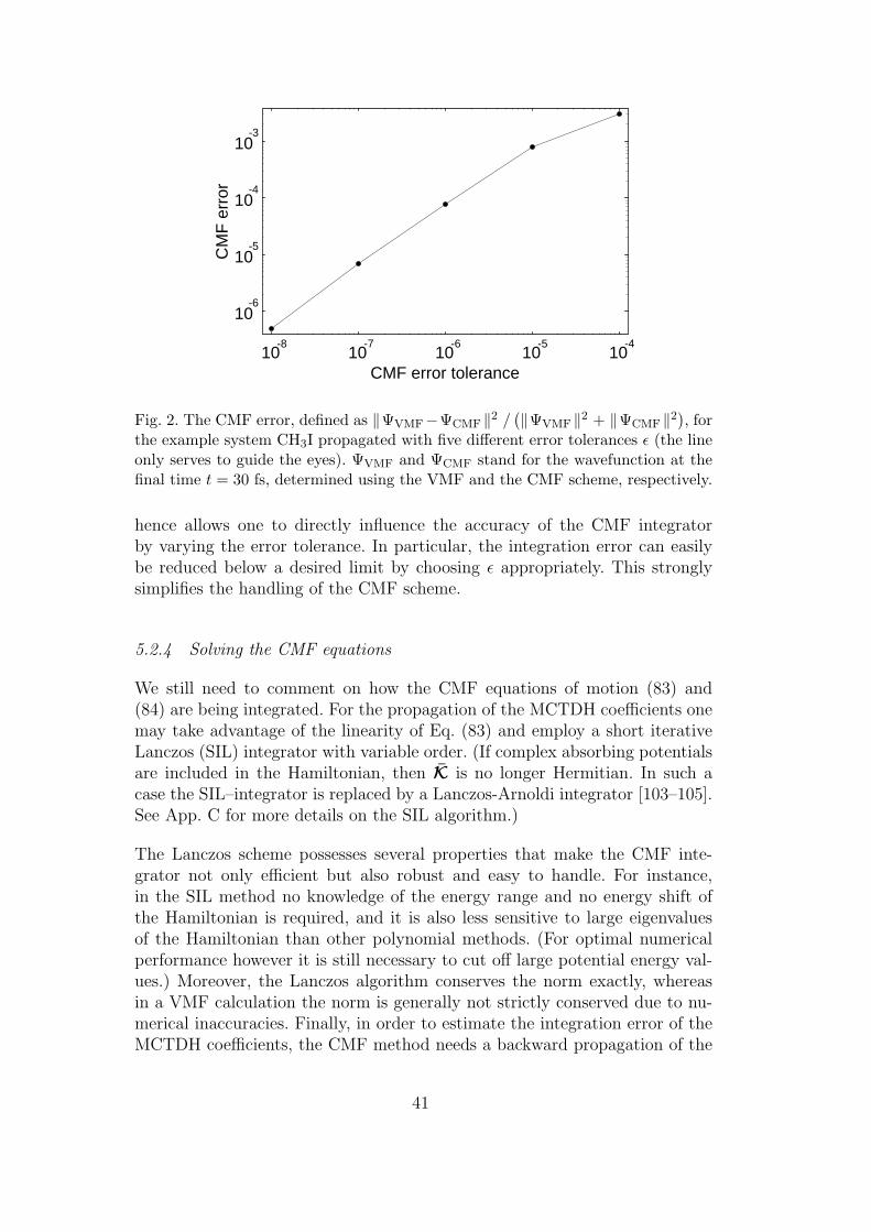
-8 10

-7 10

-6 10

-5 10

-4 10

CMF error tolerance

-6 10

-5 10

-4 10

-3 10

CM

F e

rror

Fig. 2. The CMF error, defined as ‖ΨVMF−ΨCMF ‖2 /(‖ΨVMF ‖2 + ‖ΨCMF ‖2

), for

the example system CH3I propagated with five different error tolerances ǫ (the lineonly serves to guide the eyes). ΨVMF and ΨCMF stand for the wavefunction at thefinal time t = 30 fs, determined using the VMF and the CMF scheme, respectively.

hence allows one to directly influence the accuracy of the CMF integratorby varying the error tolerance. In particular, the integration error can easilybe reduced below a desired limit by choosing ǫ appropriately. This stronglysimplifies the handling of the CMF scheme.

5.2.4 Solving the CMF equations

We still need to comment on how the CMF equations of motion (83) and(84) are being integrated. For the propagation of the MCTDH coefficients onemay take advantage of the linearity of Eq. (83) and employ a short iterativeLanczos (SIL) integrator with variable order. (If complex absorbing potentialsare included in the Hamiltonian, then K is no longer Hermitian. In such acase the SIL–integrator is replaced by a Lanczos-Arnoldi integrator [103–105].See App. C for more details on the SIL algorithm.)

The Lanczos scheme possesses several properties that make the CMF inte-grator not only efficient but also robust and easy to handle. For instance,in the SIL method no knowledge of the energy range and no energy shift ofthe Hamiltonian is required, and it is also less sensitive to large eigenvaluesof the Hamiltonian than other polynomial methods. (For optimal numericalperformance however it is still necessary to cut off large potential energy val-ues.) Moreover, the Lanczos algorithm conserves the norm exactly, whereasin a VMF calculation the norm is generally not strictly conserved due to nu-merical inaccuracies. Finally, in order to estimate the integration error of theMCTDH coefficients, the CMF method needs a backward propagation of the

41

A-vector (step 5 in Fig. 1). The SIL–integrator permits the estimation of thiserror almost for free, as the Krylov space that has to be built for this back-propagation can also be used in the subsequent forward propagation (step6).

Since Eq. (84) is non-linear, the Lanczos method cannot be applied to thesingle-particle functions. The predictor-corrector method used in the VMFscheme (see Sec. 5.1) is not very appropriate to the CMF scheme, becauseas a multistep method it must be restarted twice within each CMF step. Tointegrate Eq. (84) a Bulirsch-Stoer extrapolation method with variable orderand step size, and polynomial extrapolation [102], has been recommended [54].

In addition to the various benefits of the simplified version of the CMF schemeunderlined in Sec. 5.2.1, the second-order CMF method offers two furtheradvantages. First, the CMF integrator enables one to control the discretisationerror and adjust the step size. Without such an internal error control it wouldhardly be possible to apply the integrator to realistic problems where nothingis known about the exact solution. The second important improvement lies inincreasing the order of the error term and thus allowing larger CMF steps.

The major disadvantage of the CMF strategy compared with the simplifiedscheme discussed in Sec. 5.2.1 is the one and a half fold increase in the effortof propagating the single-particle functions. For large systems however (i.e. fornf ≫ N2) most of the computation time is typically spent on the propagationof the MCTDH coefficients, so that this additional cost is negligible.

We close this section in emphasising that the CMF integration scheme con-verges for n→ N towards the standard method (see Sec. 2.2), since for n = Nboth the single-particle functions and the mean-fields are constant. Moreover,the CMF integrator conserves the norm exactly.

5.2.5 Computational details

Attention to two numerical details significantly enhances the efficient imple-mentation of the CMF integrator.

The first one concerns the propagation of the single-particle functions accord-ing to Eq. (84). As pointed out in Sec. 4.4 this dominates the numerical cost

for small systems. Although the matrices H(κ)r are constant, the sum

s∑

r=1

H(κ)rklh

(κ)r ϕ

(κ)l (87)

still has to be computed at each evaluation of the right hand side of Eq. (84).To see how one can avoid this summation we examine the value of the vector

42

(87) at the αth (α = 1, . . . , Nκ) grid point. Let |χ(κ)α 〉 denote the correspond-

ing DVR function (see App. B). Projecting (87) onto |χ(κ)α 〉 and using the

(numerical) completeness of the set of DVR functions, we obtain

〈χ(κ)α |

s∑

r=1

H(κ)rklh

(κ)r |ϕ

(κ)l 〉 =

Nκ∑

β=1

(s∑

r=1

H(κ)rkl〈χ(κ)

α |h(κ)r |χ(κ)β 〉

)〈χ(κ)

β |ϕ(κ)l 〉 . (88)

The number in brackets could in principal be determined for all κ, α, β, k andl only once at the beginning of each CMF step and then taken from memory.However, this would require the storage of fn2N2 complex numbers. Sincemost of the single-particle operators are potential terms and hence diagonal,it seems reasonable to save only these terms and continue treating the non-diagonal ones as before. For simplicity, let us assume that the Hamiltonianexpansion terms are arranged such that the first sκ are diagonal, i.e. 〈χ(κ)

α |h(κ)r |χ

(κ)β 〉 = 〈χ(κ)

α |h(κ)r |χ(κ)α 〉δαβ, whereas the other s− sκ are represented by

full matrices. Expression (88) then reads

〈χ(κ)α |

s∑

r=1

H(κ)rklh

(κ)r |ϕ

(κ)l 〉=M

(κ)klα〈χ(κ)

α |ϕ(κ)l 〉

+s∑

r=sκ+1

H(κ)rkl〈χ(κ)

α |h(κ)r |ϕ(κ)l 〉 , (89)

with

M(κ)klα =

sκ∑

r=1

H(κ)rkl〈χ(κ)

α |h(κ)r |χ(κ)α 〉 . (90)

Since H is constant, M needs to be computed only initially at each CMF(half-) step. The numerical effort of calculating the diagonal part of sum (88)is then reduced by a factor of sκ for each degree of freedom κ, diminishing theoverhead due to the product form (64) of the residual Hamiltonian.

The second item refers to the adaptation of the step size. When the CMFintegrator is applied to realistic problems, where the interest lies in calculat-ing observable quantities, one usually needs the wavefunction Ψ at certain(typically equidistant) times tm. According to the uncertainty principle, thedistance ∆t = tm+1−tm between two neighbouring points must be chosen suffi-ciently small to resolve the full energy range. Since the step size τ is limited byτ ≤ ∆t, this might affect the length of the CMF steps and hence reduce the in-tegrator’s efficiency. In those cases where the observables are determined usingthe auto-correlation function, a simple trick exists that enables one to doublethe output interval ∆t. The preferable way to compute the auto-correlationfunction is given by Eq. (167). However, the auto-correlation function is then

43

known solely at the times 2m∆t instead of m∆t (m = 0, 1, . . .). At the inter-mediate points (2m−1)∆t the auto-correlation function can be obtained fromc((2m− 1)∆t) = 〈Ψ∗((m− 1)∆t) |Ψ(m∆t)〉, if Ψ((m− 1)∆t) has been storedin memory. This permits the choice of a ∆t which is twice as large as before.

5.2.6 Numerical effort

Having described the CMF integration scheme in detail, we shall estimate theexpected speed-up of a CMF calculation compared with a VMF calculation.We restrict our discussion to large systems (i.e. nf ≫ N2), where the dominantcontribution to the numerical effort is caused by the computation of the mean-field matrices and the time-derivative of the MCTDH coefficients. We assumethat in the VMF scheme the equations of motion are solved using a predictor-corrector routine that evaluates the differential equation twice in each step.As outlined in Sec. 4.4, this requires 2c1sf

2nf+1 floating point operations perstep, where c1 is a proportionality constant. In a CMF calculation with aLanczos integrator of mean order l used for the propagation of the MCTDHcoefficients, 2c1sf

2nf+1 + 2c2lsfnf+1 floating point operations are needed for

the two CMF half-steps. In our implementation of the code the constants c1and c2 fulfil the relation c2 ≈ 2c1. The gain of a CMF calculation with respectto a VMF calculation can hence be approximated by

gain(CMF/VMF) ≈ f

f + 2l

τCMF

τVMF

, (91)

with τCMF and τVMF being the mean CMF and VMF (i.e. predictor-corrector)step sizes, respectively. In the limit f → ∞ the gain is exclusively given bythe ratio of the CMF and the VMF step size.

We also want to estimate the gain of the CMF scheme with respect to the stan-dard method discussed in Sec. 2.2. To this end we assume that the equationsof motion of the standard method are solved employing a Lanczos integrator.The SIL step size in the standard method will then be comparable to the sizeof a CMF half-step, and the mean SIL order l will also be similar in bothschemes. (This is a rather conservative assumption since the matrix K used inthe CMF scheme generally has a smaller spectral range than the Hamiltonianmatrix employed in the standard method. This is because K is set up in thesingle-particle basis, which is better adapted to the potential than the primi-tive basis used in the standard method to represent the Hamiltonian matrix.)In the standard method the effort for each SIL step is given by c3lfN

f+1, withc3 ≈ c2. Thus one approximately obtains for the gain of a CMF calculationwith respect to the standard method:

gain(CMF/standard) ≈ 2l

f + 2l

1

s

(N

n

)f+1

. (92)

44

A more careful analysis shows that the expression nf+1 should be interpretedas f−1(

∑κ nκ)(

∏κ nκ) (and similarly for N f+1), and s should be taken as the

number of non-separable Hamiltonian terms plus f−1 times the number ofseparable one-dimensional terms.

We see that the CMF scheme is superior — with regard to the computationaleffort — to the standard method provided that the number of modes f andthe contraction efficiencies Nκ/nκ are sufficiently large. A realistic examplesystem with f = 6, N = 30, n = 5, s = 50, and l = 10 shall illustratethis. For this system a calculation using the (brute force) standard methodcan be expected to take 4300 times longer than a CMF calculation. If theCMF run requires for this system, say, two hours of CPU time, the standardmethod would then need about one year! This shows that MCTDH can makeinvestigations feasible that are impossible within the standard approach.

To complete our discussion we shall also compare the memory requirementsof both MCTDH versions (VMF and CMF) and the standard method. Sincefor small systems the memory requirements usually do not pose a problem,we confine ourselves again to large systems (i.e. nf ≫ fN2, when memory isconcerned) where the only important contribution to the memory comes fromthe A-vectors.

In the VMF scheme the predictor-corrector routine we usually use is drivenwith a fixed order P . An overall number of (P + 6) A-vectors must then beheld in memory (including all auxiliary vectors), yielding (P + 6)nf complexnumbers. Taking into account all A-vectors employed in the propagation, thestep size control, the additional output of the auto-correlation function, as wellas all auxiliary vectors, the CMF method requires the storage of (L + 6)nf

complex numbers, where L is the maximum Lanczos order needed to integratethe intervals of length τ/2. Typical values for the integration order are P = 6and L = 5 to L = 25.

On the other hand, in the standard approach with a Chebyshev integrator[62] taken for the propagation, four wavefunctions, i.e. 4N f complex numbers,must be stored in memory. So the memory gain of the MCTDH scheme withrespect to the standard method, defined as the ratio between the memoryrequirements, ranges from about 1/8 (N/n)f to 1/3 (N/n)f . Typically, n isabout three to ten times smaller than N , leading to impressive memory gainfactors if f is comparatively large.

For the above example system — assuming double precision arithmetics —the standard method would require the storage of 43 Gigabytes of data, whichwould by far exceed the memory of even the largest (single processor) machinesavailable today. On the contrary, the MCTDH algorithm with, say, L = 20needs merely 6 Megabytes, allowing to do the same calculation on a smallworkstation or even a personal computer!

45

5.2.7 Experiences with the CMF scheme

In order to illuminate the characteristics of the CMF integrator, let us sum-marise the experiences that have been made so far with the CMF scheme.These experiences are based on studies on the photo-dissociation of NOCl[106] and CH3I [54], the reactive scattering of H + H2 and H + D2 [45,46],the photo-absorption of pyrazine [36,37], and the scattering of N2 on an LiFsurface [107]. A detailed investigation of the CMF method can be found inRef. [54].

In these calculations the CMF error control was found to adjust the step sizevery reasonably. One aspect that has been examined is the accuracy of theCMF integrator in dependence of the chosen error tolerance ǫ. The findingwas more or less the same for all the systems mentioned above: one typicallyobtains a good, excellent, and perfect agreement between the CMF and theVMF results for ǫ = 10−5, ǫ = 10−6, and ǫ = 10−7, respectively. This consider-ably simplifies the usage of the CMF integrator since it allows one to predictquite reliably the error tolerance necessary for a desired accuracy. The numberof steps that had to be repeated because of a too large error was small in allthese calculations.

In one study [54] the CMF error was monitored during the propagation andfound to grow almost linearly with the propagation time. The CMF error wasalso compared with the MCTDH error, i.e. the error of the MCTDH schemewith respect to the standard method (see Sec. 2.2). The CMF error was slightlysmaller than the MCTDH error when ǫ = 10−6 was used, and negligible forǫ = 10−7. Furthermore, in all calculations with a Hermitian Hamiltonian theCMF method conserves the norm very strictly, because the SIL integratorexplicitly constructs a normalised solution. Employing the VMF scheme, onthe other hand, generally leads to a slight loss of norm due to numericalinaccuracies.

Another interesting property is of course the gain of the CMF over the VMFscheme. As explained in Sec. 5.2.6 one can expect a considerable reductionof the CPU time for systems for which the computation of the mean-fieldsis expensive, i.e. for systems with many degrees of freedom f (or particlesp when modes are combined, see Sec. 4.5), many single-particle functions n,and a large number of Hamiltonian expansion terms s. In several studies thisgain amounted to about a factor of ten, with virtually no loss of accuracy[54,45,46]. For the 24-mode pyrazine system [36,37] it is not manageable toperform a VMF run over the full propagation time, so the integration schemeswere compared over only a short initial time segment; gain factors between 10and 20 were then obtained. The CMF method was even for the rather smallNOCl system (f = 3, n = 5, s = 22) about three times faster than the VMFscheme (see Sec. 9.1). The memory requirement of the CMF calculations,

46

which mainly depends on the maximum Lanczos order, was nearly alwayscomparable to that of the VMF method.

So far only one example — the scattering of N2 on an LiF surface — hasbeen found where the use of the CMF integrator led to only an insignificantreduction of the computation time, so that the VMF method was preferred[107]. In that study the spherical harmonics FBR was employed (cf. App.B.4.6) yielding non-diagonal potential matrices. This disables the summationof potential terms as discussed in Sec. 5.2.5, making the CMF scheme lessefficient for this special case.

The studies that have been performed to date indicate that for sufficientlylarge systems the CMF integration scheme usually reduces the computationaleffort by one order of magnitude. Therefore, the CMF scheme has turned outto be the favoured integrator for large systems.

47

6 Product representation of potential energy surfaces

The knowledge of the electronic potential energy surface (PES) of the molec-ular system under consideration is a necessary prerequisite when investigatingmolecular dynamics. The PES may be given on a grid of, e.g. ab initio, points,or there may exist an analytical fit or a model potential which representsthe PES. These representations are, by their nature, multi-dimensional andnon-separable. The MCTDH algorithm, however, requires the potential to berepresented as a linear combination of products of one-dimensional functions(except when employing the CDVR method, see Sec. 4.3).

In this section algorithms are discussed that allow the generation of suchproduct representations. The product representation should converge fast, i.e.should require only a small number of expansion terms for representing thepotential within some error bound. For more detailed discussions on productrepresentation algorithms see Refs. [40,56,57].

6.1 Expansion in natural potentials

Given a real and continuous function of two variables the Approximationsthe-orem of Schmidt defines a constructive scheme to approximate this functionas a sum of products of one-dimensional functions [108]. This approximationis proven to be optimal in the L2-sense. The approximation procedure requiresthe computation of the eigenvalues and eigenfunctions of an integral kernel ofa homogeneous integral equation. Extending this ansatz to an arbitrary num-ber of degrees of freedom is the basis of the product representation schemewhich is outlined in the following.

First, the potential energy values Vi1...if are assumed to be given on a productgrid,

V(Q

(1)i1 , . . . , Q

(f)if

)≡ Vi1...if , (93)

where f denotes the number of degrees of freedom considered and Q(κ) thecoordinate of the κth degree of freedom. Finally, Q

(κ)iκ denotes the iκth grid

point of the κth one-dimensional grid with 1 ≤ iκ ≤ Nκ. The grids are preciselythe grids used in the subsequent MCTDH calculation.

Next, symmetric positive semi-definite potential density matrices (κ) are de-fined:

(κ)jl =

N1∑

i1=1

. . .Nκ−1∑

iκ−1=1

Nκ+1∑

iκ+1=1

. . .Nf∑

if=1

Vi1...iκ−1jiκ+1...ifVi1...iκ−1liκ+1...if . (94)

48

The orthonormal eigenvectors v(κ)j (with components v

(κ)ij ) and the eigenval-

ues λ(κ)j of the potential density matrix (κ) are called natural potentials and

natural potential populations, respectively. The natural populations are as-sumed to be in decreasing order, λ

(κ)j ≥ λ

(κ)j+1, and it is convenient to introduce

the notation v(κ)j (Q

(κ)i ) := v

(κ)ij . This notation interprets the eigenvectors v

(κ)j

as one-dimensional functions which, however, are defined on the set of gridpoints Q(κ)

i only. Choosing a set of expansion orders mκ one may nowapproximate the potential

V(Q

(1)i1 , . . . , Q

(f)if

)≈V app

(Q

(1)i1 , . . . , Q

(f)if

)

=m1∑

j1=1

. . .mf∑

jf=1

Cj1...jf v(1)j1

(Q

(1)i1

). . . v

(f)jf

(Q

(f)if

). (95)

The expansion coefficients Cj1...jf are determined by the overlaps between thepotential and the natural potentials,

Cj1...jf =N1∑

i1=1

. . .Nf∑

if=1

Vi1...ifv(1)i1j1 . . . v

(f)if jf

. (96)

Since the orthonormal product basis set is complete over the grid points,we find that the approximated and the exact potential are identical at thegrid points, if the expansion orders and the number of grid points are equal,i.e, V app → V for mκ → Nκ. Note that the expansion coefficients areindependent of the expansion orders.

The two-dimensional case is a special one. Here, the two potential densitymatrices have identical eigenvalues (except for possibly a different number ofzero eigenvalues). The coefficient matrix is diagonal [27,29],

Cij = ±δij√λi , (97)

and the expansion is optimal, i.e. the L2-error of the approximation is minimal(see Approximationstheorem by E. Schmidt [108]).

The L2-error ∆2 is defined as the sum of the squares of the moduli of the fiterrors on all product grid points,

∆2 =N1∑

i1=1

. . .Nf∑

if=1

(Vi1...if − V app

i1...if

)2. (98)

For an arbitrary number of degrees of freedom it is shown in App. D that theL2-error ∆2 can be expressed in terms of the expansion coefficients,

49

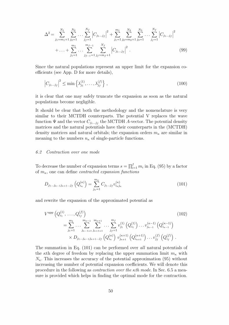
∆2 =N1∑

j1=m1+1

N2∑

j2=1

. . .Nf∑

jf=1

∣∣∣Cj1...jf

∣∣∣2+

m1∑

j1=1

N2∑

j2=m2+1

N3∑

j3=1

. . .Nf∑

jf=1

∣∣∣Cj1...jf

∣∣∣2

+ . . .+m1∑

j1=1

. . .mf−1∑

jf−1=1

Nf∑

jf=mf+1

∣∣∣Cj1...jf

∣∣∣2. (99)

Since the natural populations represent an upper limit for the expansion co-efficients (see App. D for more details),

∣∣∣Cj1...jf

∣∣∣2 ≤ min

λ(1)j1 , . . . , λ

(f)jf

, (100)

it is clear that one may safely truncate the expansion as soon as the naturalpopulations become negligible.

It should be clear that both the methodology and the nomenclature is verysimilar to their MCTDH counterparts. The potential V replaces the wavefunction Ψ and the vector Cj1...jf the MCTDH A-vector. The potential densitymatrices and the natural potentials have their counterparts in the (MCTDH)density matrices and natural orbitals; the expansion orders mκ are similar inmeaning to the numbers nκ of single-particle functions.

6.2 Contraction over one mode

To decrease the number of expansion terms s =∏f

i=1mi in Eq. (95) by a factorof mκ, one can define contracted expansion functions

Dj1...jκ−1jκ+1...jf

(Q

(κ)iκ

)=

mκ∑

jκ=1

Cj1...jfv(κ)iκjκ (101)

and rewrite the expansion of the approximated potential as

V app(Q

(1)i1 , . . . , Q

(f)if

)(102)

=m1∑

j1=1

. . .mκ−1∑

jκ−1=1

mκ+1∑

jκ+1=1

. . .mf∑

jf=1

v(1)j1

(Q

(1)i1

). . . v

(κ−1)jκ−1

(Q

(κ−1)iκ−1

)

×Dj1...jκ−1jκ+1...jf

(Q

(κ)iκ

)v(κ+1)jκ+1

(Q

(κ+1)iκ+1

). . . v

(f)jf

(Q

(f)if

).

The summation in Eq. (101) can be performed over all natural potentials ofthe κth degree of freedom by replacing the upper summation limit mκ withNκ. This increases the accuracy of the potential approximation (95) withoutincreasing the number of potential expansion coefficients. We will denote thisprocedure in the following as contraction over the κth mode. In Sec. 6.5 a mea-sure is provided which helps in finding the optimal mode for the contraction.

50

6.3 Iterative optimisation

In contrast to the two-dimensional case the expansion (95) is in general notoptimal for more than two degrees of freedom, and there may exist anotherproduct basis for which the L2-error may be smaller for the same set of ex-pansion orders mκ. In order to arrive at these optimal potential functionsone may iteratively improve the natural potentials by a multi-dimensionaloptimisation procedure.

Since the natural potentials form a complete set in which to represent thepotential on the grid points, one can define the following ansatz for improvedvectors v

(κ)j of the κth degree of freedom,

v(κ)j = v

(κ)j +

Nκ∑

l=mκ+1

µ(κ)jl v

(κ)l , j = 1, 2, . . . ,mκ , (103)

where v(κ)j denotes the natural potentials obtained by diagonalisation of the

density matrix (κ) (see Eq. (94)) and where mκ and Nκ are the expansionorder and the number of grid points for the κth degree of freedom, respectively.

The parameters µ(κ)jl may be understood as the unknown model parameters of

a merit function χ2,

χ2(µ) =N1∑

i1=1

. . .Nf∑

if=1

(Vi1...if − V app

i1...if

)2, (104)

which is to be minimised with respect to µ, where µ denotes the setµ(κ)

of

µ-matrices for each degree of freedom. The new representation of the potentialin the basis of the new fit vectors is then given by

V appi1...if

=m1∑

j1=1

. . .mf∑

jf=1

Cj1...jf v(1)i1j1 . . . v

(f)if jf

, (105)

with the expansion coefficients Cj1...jf defined as in Eq. (96) by the overlaps

of the improved (and re-orthonormalised) vectors v(κ)j with the potential V .

This nonlinear optimisation problem may be written as a set of linear equa-tions for the parameters µ(κ) involving the calculation of the gradient andof the Hessian matrix of χ2 with respect to µ(κ). The solution of this set oflinear equations defines improved vectors according to Eq. (103) which can be

iteratively optimised repeating the same procedure until the µ(κ)jl coefficients

become sufficiently small (for further details see Ref. [102]).

51

We prefer a different approach to iteratively improve the natural potentials,and thereby to minimise the L2-error of the approximated potential energysurface as given by Eq. (99). The iteration scheme described in the followingcan be shown to be equivalent to the above-mentioned procedure, but webelieve it is more stable and easier to implement.

Before the iteration scheme is outlined, modified potential density matrices˜(κ) are introduced:

˜(κ)jl =

m1∑

j1=1

. . .mκ−1∑

jκ−1=1

mκ+1∑

jκ+1=1

. . .mf∑

jf=1

Cj1...jκ−1jjκ+1...jfCj1...jκ−1ljκ+1...jf . (106)

The indices j and l run from 1 to Nκ such that the short potential coefficientvector Cj1...jf of Eq. (95), where 1 ≤ jκ ≤ mκ, is replaced by a long coefficientvector without index restriction. Note that in contrast to Eq. (94) the uppersummation limits are the potential expansion orders mκ and not the numberof grid points Nκ. If the potential expansion orders mκ equal the number ofgrid points Nκ in each degree of freedom, then the modified potential densitymatrix ˜(κ) becomes identical to the diagonalised form of the original potentialdensity matrix (κ), i.e. ˜

(κ)ij → δijλ

(κ)j for mκ → Nκ. By diagonalising the

modified potential density matrix ˜(κ) one arrives at an L2-optimal separationbetween the κth degree of freedom and the rest as currently approximated.Running through all the degrees of freedom one will eventually converge to aglobal L2-optimal product representation.

The individual steps of the iteration scheme can now be summarised:

(1) Start of iteration: For each degree of freedom the potential density matri-

ces (κ) are diagonalised, and all natural potentials v(κ)jκ (1 ≤ jκ ≤ Nκ) are

computed.(2) For each degree of freedom the natural potentials are copied according to

vold,(κ)jκ := v

(κ)jκ .

All following steps are performed successively for each degree of freedom κ.(3) The long vector of coefficients Cj1...jf , with 1 ≤ jκ ≤ Nκ, is computed as the

overlap of the old potential vectors with the potential V (see Eq. (96))

Cj1...jf =N1∑

i1=1

. . .Nf∑

if=1

Vi1...ifvold,(1)i1j1 . . . v

old,(f)if jf

. (107)

(4) The modified potential density matrices ˜(κ) are computed according to Eq.(106) and diagonalised:

˜(κ)diag = U

(κ)T ˜(κ)U (κ) . (108)

U (κ) denotes the orthogonal matrix of eigenvectors of the κth degree offreedom.

52

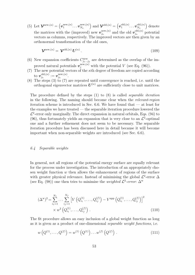
(5) Let Vnew,(κ) =(vnew,(κ)1 . . .v

new,(κ)Nκ

)and V

old,(κ) =(vold,(κ)1 . . .v

old,(κ)Nκ

)denote

the matrices with the (improved) new vnew,(κ)jκ and the old v

old,(κ)jκ potential

vectors as columns, respectively. The improved vectors are then given by anorthonormal transformation of the old ones,

Vnew,(κ) = V

old,(κ)U (κ) . (109)

(6) New expansion coefficients Cnewj1...jf

are determined as the overlap of the im-

proved natural potentials vnew,(κ)j with the potential V (see Eq. (96)).

(7) The new potential vectors of the κth degree of freedom are copied according

to vold,(κ)jκ := v

new,(κ)jκ .

(8) The steps (3) to (7) are repeated until convergence is reached, i.e. until theorthogonal eigenvector matrices U (κ) are sufficiently close to unit matrices.

The procedure defined by the steps (1) to (8) is called separable iterationin the following. The naming should become clear when the relevant-regioniteration scheme is introduced in Sec. 6.6. We have found that — at least forthe examples we have treated — the separable iteration procedure lowered theL2-error only marginally. The direct expansion in natural orbitals, Eqs. (94) to(96), thus fortunately yields an expansion that is very close to an L2-optimalone and a further refinement does not seem to be necessary. The separableiteration procedure has been discussed here in detail because it will becomeimportant when non-separable weights are introduced (see Sec. 6.6).

6.4 Separable weights

In general, not all regions of the potential energy surface are equally relevantfor the process under investigation. The introduction of an appropriately cho-sen weight function w then allows the enhancement of regions of the surfacewith greater physical relevance. Instead of minimising the global L2-error ∆(see Eq. (98)) one then tries to minimise the weighted L2-error: ∆w

(∆w)2 =N1∑

i1=1

. . .Nf∑

if=1

[V(Q

(1)i1 , . . . , Q

(f)if

)− V app

(Q

(1)i1 , . . . , Q

(f)if

)]2

× w2(Q

(1)i1 , . . . , Q

(f)if

). (110)

The fit procedure allows an easy inclusion of a global weight function as longas it is given as a product of one-dimensional separable weight functions, i.e.

w(Q(1), . . . , Q(f)

)= w(1)

(Q(1)

). . . w(f)

(Q(f)

). (111)

53

The variational problem (110) is then equivalent to a global L2-error minimi-sation of the weighted potential energy surface

V wi1...if

= V(Q

(1)i1 , . . . , Q

(f)if

)· w(1)

(Q

(1)i1

). . . w(f)

(Q

(f)if

), (112)

which can be expanded in a natural potential basis as defined by Eq. (95).The approximated potential surface then reads as

V appi1...if

=m1∑

j1=1

. . .mf∑

jf=1

Cwj1...jf

(vw,(1)i1j1 /w

(1)i1

). . .(vw,(f)if jf

/w(f)if

), (113)

where vw,(κ) and Cwj1...jf

denote the natural potentials and expansion coeffi-

cients derived from the weighted potential energy surface V w, Eq. (112), and

where w(κ)j = w(κ)(Q

(κ)j ).

Separable weights have been successfully applied in the product representationof the S1-surface of NOCl. There an appropriate choice of the separable weightsled to a reduction of the number of necessary expansion terms by a factor ofabout five [56].

6.5 Error measures

So far we have defined the quality of a potential fit by its (global) L2-error.After weights have been introduced more refined error measures are necessary.

By ∆wrms we denote a weighted root-mean-square (rms) error which is defined

as

∆wrms =

√√√√√S−1N1∑

i1=1

. . .Nf∑

if=1

(Vi1...if − V app

i1...if

)2w

(1)2

i1 . . . w(f)2

if, (114)

where

S =N1∑

i1=1

. . .Nf∑

if=1

w(1)2

i1 . . . w(f)2

if. (115)

Introducing reduced natural populations,

λred = λ/S , (116)

54

both the reduced natural populations λred and the weighted rms-error ∆wrms

are invariant with respect to a multiplication of the weight functions by aconstant scale factor.

If all weights equal 1, i.e. w(κ)i ≡ 1, S equals the number of grid points Ntot =∏f

κ=1Nκ and ∆wrms reduces to the (common) global rms-error

∆rms =

√√√√√N−1tot

N1∑

i1=1

. . .Nf∑

if=1

(Vi1...if − V app

i1...if

)2. (117)

The reduced natural populations and the weighted rms-error are closely re-lated. If one removes from a complete expansion (i.e. mκ = Nκ) in one degreeof freedom exactly those m natural potentials which correspond to the m low-est natural potential populations, one can immediately specify the resultingweighted rms-error [56]:

∆wrms =

√√√√√Nκ∑

j=Nκ−m

λred,(κ)j . (118)

Equation (118) may be generalised by summing over all those reduced nat-ural populations corresponding to those natural potentials which have beenremoved from the expansion (95). This quantity still provides a good estimatefor the resulting rms-error,

∆wrms ≈

√√√√√f∑

κ=1

Nκ∑

jκ=mκ+1

λred,(κ)jκ . (119)

This estimate is very helpful when choosing the potential orders, mκ.

For two dimensions the approximation error can be expressed exactly, sincethe coefficient matrix of the product expansion in this case is diagonal (seeEq. (97)). Employing Eq. (118) one obtains in this case

∆wrms =

√√√√√min (N1,N2)∑

j=s+1

λredj , (120)

where s = m1 = m2 denotes the expansion order and N1 and N2 the numberof grid points of the first and second degree of freedom, respectively.

Since the approximation error for given expansion order s in general is notindependent of the degree of freedom over which the contraction (see Eq.

55

(102)) is performed it is important to choose the optimal degree of freedomfor contraction. The reduced natural potential populations, as defined in Eq.(116), provide good criteria for choosing the optimal degree of freedom forcontraction. Following the lines which led to the estimation Eq. (119) theoptimal degree of freedom for contraction is that for which the measure

(∆(κ)

)2=

f∑

κ′=1

κ′ 6=κ

Nκ′∑

j=mκ′+1

λred,(κ′)j (121)

is minimal.

6.6 Emulating non-separable weights

More efficient than separable weights are of course general non-separableweights. The direct application of non-separable weights (see, e.g., chapter15.5 of Ref. [102]), however, results in (often unsolvable) large coupled sys-tems of linear equations. To circumvent this problem we emulate non-separableweights by modifying the potential to be approximated. To this end an f -dimensional function ω is introduced which assigns every potential value onthe product grid a weight between 0 and 1,

0 ≤ ωi1...if ≡ ω(Q

(1)i1 , . . . , Q

(f)if

)≤ 1 . (122)

All physically relevant points are given the weight 1 and all physically less oreven irrelevant points are given smaller weights or even the weight 0.

Having defined ω, the separable iteration procedure of Sec. 6.3 can be modifiedand extended in such a way that f -dimensional non-separable weight functionscan be simulated. The concept and the individual steps of this relevant regioniteration are described in the following.

To begin with, the exact potential V is expanded in the standard manner in aproduct basis of natural potentials according to Eq. (95), yielding V app. Thena modified reference potential V is defined as a linear combination of the exactpotential V and of the potential fit V app,

Vi1...if = ωi1...ifVi1...if + (1− ωi1...if )Vappi1...if

. (123)

The modified reference potential V equals the exact potential at points whereω = 1, and becomes the fit-potential V app when ω = 0. In the following themodified reference potential V serves as the new reference potential whichis to be approximated. To this end a single iteration step, as described in

56

detail in Sec. 6.3 is performed. As a result of this iteration step, improvedone-dimensional potential vectors and corresponding potential expansion co-efficients are determined. Improved means that the L2-error over the relevantregion is reduced.

The individual steps of the relevant region iteration procedure can be repeateduntil some break-off criterion is satisfied. After each step the representationof the exact potential energy surface in the relevant region is improved.

Schematically the relevant region iteration procedure can be summarised asfollows:

(0) Initialisation:• The relevant regions and therewith the f -dimensional function ω are defined.• The exact potential V is expanded in a product basis of natural potentialsaccording to Eq. (95), yielding V app.

• The counter is set to k = 0, and V(0),appi1...if

= V appi1...if

.(1) The modified reference potential is defined:

V(k+1)i1...if

= ωi1...ifVi1...if + (1− ωi1...if )V(k),appi1...if

. (124)

(2) One separable iteration step as defined in Sec. 6.3 is performed. The onlymodification is that the exact potential V is replaced by the modified ref-erence potential V (k+1). V (k+1),app then denotes the product representationof V (k+1).

(3) The step counter is increased by one: k ← k + 1.(4) The steps (1) to (3) are repeated until some break-off criterion is satisfied.

The interpretation of the f -dimensional function ω (see Eq. (122)) can besubstantially extended assuming that the relevant region iteration converges.In fact, in all examples investigated so far the relevant region iteration con-verged (as long as ω > 0) even though the convergence property has not yetbeen proven in a strict mathematical sense. In the limit of convergence boththe modified reference potential and the approximated potential by definitionstay constant, i.e. limk→∞ V (k+1) = V and limk→∞ V (k),app = V app hold.

For these converged quantities it follows immediately from Eq. (124) that

Vi1...if − V appi1...if

= ωi1...if

(Vi1...if − V app

i1...if

). (125)

Since the iteration procedure minimises the difference (in L2-sense) betweenthe approximated potential V app and the modified reference potential V , itminimises the weighted difference appearing on the right hand side of Eq.(125). Thus, it minimises the weighted L2-error ∆w defined by Eq. (110) fora general multi-dimensional weight function with ω replacing w.

57

Since we may now consider ω as a general weight function, the use of separa-ble weights seems to be redundant. However, we prefer to keep the separableweights. Their use allows ω to be defined by a simple, vivid, and convenientprocedure, namely by defining relevant regions where ω = 1. Since the refer-ence potential is not changed over the relevant region, the iteration procedureconverges faster than in cases where ω takes on a complicated form. Addi-tionally, the use of separable weights, with the aid of Eq. (119), provides aconvenient tool for determining the optimal expansion orders mκ.

To monitor the performance of the relevant-region iteration procedure addi-tional error measures are introduced. The relevant rms-error ∆r

rms and therelevant and weighted rms-error ∆rw

rms are defined similarly to Eqs. (117) and(114) but the summations now run only over the relevant grid points, i.e. thosepoints for which ωi1...if = 1 holds.

6.7 Concluding remarks

The product representation scheme of potential energy surfaces outlined in thepreceding sections has been mainly developed in order to represent (analyti-cally) given potential energy surfaces in an MCTDH adapted product form.It should be noted though that the procedure itself is general, and is by nomeans restricted to being employed in connection with MCTDH.

In cases where the potential energy surface is not given analytically, but thepotential values are provided on a product grid (i.e. as a set of ab initiopoints) the product representation scheme can also be used to interpolatemulti-dimensional potential energy surfaces (see Ref. [56] for more details).

Another point worth mentioning is that exploiting the underlying symmetry ofthe potential under consideration can substantially reduce the computationaleffort in terms of CPU time and memory. This has been shown in Ref. [56] inthe example of a Coulomb potential.

6.8 Applications

In order to illustrate the product representation scheme of potential energysurfaces, we will give some example calculations. The first one treats the S1-potential energy surface used for the photo-dissociation process of NOCl [56].The product representation scheme has also been extensively employed todescribe two- and three-dimensional reactive scattering of H+H2 and its iso-topic variants in binding [40,109], Jacobian [45,46,57,109], and hyperspherical[41,42] coordinates. We will review some of these studies.

58

6.8.1 The S1-surface of NOCl

The product representation of the three-dimensional S1-potential energy sur-face of NOCl served as one of the first realistic examples [56]. The potentialenergy surface of Schinke et al. [110] was used which is given as a cubic-splinefit to more than 600 ab initio points.

To check the quality of different product representations, MCTDH photo-dissociation calculations were performed and photo-absorption spectra weredetermined [56]. Without using weights, about 100 expansion coefficients werenecessary in order to accurately reproduce the spectra obtained by propagationon the Schinke surface [56]. Here, the contraction (see Sec. 6.2) was performedover the angular degree of freedom.

Employing separable weights as defined in Sec. 6.4 the number of expansioncoefficients could be reduced. Only 20 expansion coefficients were then found tobe necessary. Note that this reduction of the number of expansion coefficientsby a factor of five speeds up the MCTDH calculation by almost the samefactor.

The choice of the separable weights was straightforward and intuitive. For ex-plicit parameters and functional forms of the separable weight functions thereader is referred to Ref. [56]. The parameters presented in that reference justserve as an example, and can be varied without causing drastic changes. Theweight function for the dissociative degree of freedom reduces the importanceof the high energy repulsive part of the surface corresponding to small dis-tances of the dissociative coordinate. The two other weight functions furtherpronounce those regions of the potential energy surface which the wavepacketvisits during the photo-dissociation process.

6.8.2 The collinear LSTH-surface

The product representation of the collinear Liu-Siegbahn-Truhlar-Horowitz(LSTH) surface [111–113] was studied in both Jacobian and binding coordi-nates. This example demonstrates that the choice of the coordinate systemmay strongly influence the rate of convergence of the product representation.

A second point studied here is the relevant region iteration procedure describedin Sec. 6.6. By separating the coordinate space into regions of minor and majorphysical relevance the surface is no longer globally optimised, but specificallyoptimised in the regions of major physical relevance.

The definition of the relevant regions is not only dependent on the surfacebut also on the process to be described. The energy distribution of the ini-tial wavepacket defines those regions of the potential energy surface which areenergetically accessible for the propagated wavepacket. Thus, for all potential

59

binding coordinates Jacobian coordinates

Error- s = 10 s = 20 s = 10

measures sep. weight rel. reg. sep. weight rel. reg. sep. weight rel. reg.

∆rwrms 0.13 0.04 0.05 0.01 15.4 3.65

∆rrms 0.44 0.14 0.18 0.04 53.1 12.7

∆rms 1.08 2.91 0.26 0.34 83.0 111

∆rmax 1.90 0.70 1.37 0.35 428 97.8

∆max 4.54 13.8 1.95 2.62 857 1083

Table 1Errors in meV of three product representations of the collinear LSTH-surface. Theerror measures are defined by Eqs. (114) to (117). ∆max denotes the maximum en-ergy difference over all grid points. The upper index r indicates that the error ∆is evaluated over the relevant region only. The number of potential terms includedis denoted by s and the labels “sep. weight” and “rel. reg.” denote that separa-ble weights only and separable weights plus relevant region iteration have beenemployed, respectively.

regions with energies greater than some energy Erel, the function ω (Eq. (122))takes small or even zero values. Additionally, in regions covered by complexabsorbing potentials (CAPs), the wavepacket is absorbed artificially and thepotential there does not need to be represented as accurately as in the inter-action region. The thus defined relevant region [81] covers about 30% of allgrid points.

The relevant region iteration procedure impressively improves the represen-tation of the surface in the relevant region. Some numbers may highlight theimprovements obtained after about 20 to 50 iteration steps. For both coordi-nate systems all relevant error measures (∆rw

rms, ∆rrms, ∆

rmax) are reduced by

about a factor of 3 to 5. At the same time the representation in the regions ofminor relevance remained acceptable (see Tab. 1).

We now discuss the impact of the chosen coordinate system on the convergenceof the product representation. This impact is indeed considerable. For the sameexpansion order the error for the representation in Jacobian coordinates isabout two orders of magnitude larger. For 10 expansion coefficients, for exam-ple, the relevant and weighted rms-errors of the representation in binding andin Jacobian coordinates accounts to ∆rw

rms = 0.04 meV and ∆rwrms = 3.65 meV,

respectively. The latter number drops to 0.01 meV when 20 expansion coeffi-cients are employed. A representation in Jacobian coordinates hence requiresabout twice as many expansion coefficients as a representation in binding co-ordinates. Finally, Tab. 1 compiles the values of the different error measures

60

for the various cases. Reference [81] provides a more detailed discussion on theproduct representation of the collinear LSTH surface.

6.8.3 The 3D LSTH surface

The influence of product expansions of differing accuracy on the quality ofthree-dimensional H+H2 reactive scattering calculations for total angular mo-mentum J = 0 has been investigated in detail in Ref. [57]. There reactionprobabilities obtained from MCTDH wavepacket propagation calculations ondifferent surfaces are compared with numerically exact results of Zhang et al.[114].

The definition of the relevant regions followed the lines given in the precedingsection. On satisfying the constraints defined in Ref. [57], again about 30% ofall grid points are located in the relevant potential region. Separable weightswhich pronounce the reaction channels and collinear configurations were em-ployed. The contraction was performed over the dissociative degree of freedomafter analysing the measure ∆(κ) (see Eq. (121)).

For an expansion with 240 terms the relevant and weighted rms-error, ∆rwrms, is

reduced from 5.3 to 1.0 meV after 30 iteration steps. A very accurate represen-tation is thus generated. Only 60 expansion terms were found to be required toobtain converged H+H2(ν=j=J=0) reaction probabilities for total energiesup to 2 eV. Only 108 expansion coefficients were needed for H+D2 coupledstates calculations of initial state-selected reaction cross-sections [46]. Some ofthese coupled states results are presented in Sec. 9.2.

The numerical effort required for determining the product representation iscomparatively small. It took about two minutes on an AIX RS/6000 power2workstation to compute the 240-terms potential approximation. This timingincludes all iteration steps and the (comparatively time consuming) calculationof the different error measures after each iteration.

61

7 Preparation of the initial wavepacket

As outlined in the introduction, solving the time-dependent Schrodinger equa-tion by a wavepacket propagation method requires the generation of an initialstate. The definition of the initial state depends on the physical process underconsideration, whereas its representation must fit the form of the MCTDHwavefunction (19). In some cases the initial wavefunction has a simple prod-uct form, e.g. a Hartree product, and can therefore be used directly. In othercases it is necessary to generate a complicated initial wavefunction. In the fol-lowing sections two methods are described which generate commonly needed,complicated initial wavefunctions.

7.1 Generation of eigenstates by energy relaxation

In many processes the initial state is the eigenfunction of a potential en-ergy surface. For example, in applications which involve a transition fromthe electronic ground to an excited state, the initial function is the ground-state eigenfunction of the system placed on an excited electronic state energysurface. Such an eigenfunction can be generated by applying the method ofenergy relaxation to a guess function [115]. In this method the wavefunc-tion is propagated in imaginary time t = −iτ . In Eq. (1) the exponentialexp(−iEjt) is thus replaced by exp(−Ejτ), and the high energy contributionsof the wavefunction are damped out. Performing this relaxation using the MC-TDH method automatically generates the eigenfunction in the desired form.Energy relaxation was hence the method of choice in the MCTDH studies onthe photo-dissociation of NOCl [28], NO2 [31], and CH3I [32,33,54].

Conventionally, during relaxation the wavefunction must be regularly renor-malised to compensate for the loss of norm. When a relaxation calculation isperformed within the MCTDH framework, the constraint g(κ) = 0 is used andit is sufficient to renormalise the MCTDH coefficients AJ only. This is becausethe single-particle functions remain orthonormalised even for imaginary timesdue to the position of the projection operator in Eq. (41). For the A-vectorone has to employ the equation of motion (68) and imaginary times or, equiv-alently, to use the equation A = −KA and real times. However, we foundit convenient to slightly modify this working equation and use the non-linearequation

A = − (K− E1)A with E =〈A | K | A〉〈A | A〉 (126)

instead. The wavefunction then still converges to the lowest eigenfunction ofthe Hamiltonian, but automatically stays normalised.

62

The main advantage of performing a relaxation calculation in this manner is atechnical one: renormalisation is somewhat tricky when using a multistep inte-gration routine, as is typically used in the VMF integration scheme (Sec. 5.1),because the wavefunctions at previous times have to be modified accordingly.

Note that since Eq. (126) is non-linear it cannot be solved with the SIL scheme,which is the preferable integrator in the CMF approach (Sec. 5.2). When theLanczos scheme is employed in the relaxation of the MCTDH coefficients wetherefore compute E only before each SIL step and renormalise A afterwards.

7.2 Initial wavepacket correction schemes for scattering problems

In scattering calculations the initial wavepacket can often be written as aHartree product undergoing free motion in the reactant asymptotic region ofthe potential energy surface. This region is however often far away from thescattering centre, and long propagation times are then required. Here, cor-rection schemes are detailed which enable the initial wavepacket to be movedcloser to the centre, while retaining the product form required by the MCTDHmethod. The schemes have been used in a study on the H+H2 (D2) reactivescattering system [45,46]. Although having been developed for MCTDH, thesecorrections can be useful for other propagation schemes as well.

7.2.1 Preliminaries

Before the correction schemes are detailed, some definitions and concepts arebriefly reviewed. A coordinate system is assumed where R denotes the distancebetween the two scattering fragments and x collectively denotes all the othercoordinates. The Hamiltonian of the scattering system is then written as

H = H0 + VI , (127)

where VI = VI(R,x) denotes the interaction potential which may contain acentrifugal term. It vanishes for large values of R,

limR→∞

VI(R,x) = 0 . (128)

The free Hamiltonian

H0 = TR +Hint (129)

is the sum of the kinetic energy of the relative motion of the fragments,TR = −(2µR)

−1∂2/∂R2, and the internal Hamiltonian Hint that operates on

63

the internal coordinates x only. The spectrum of the internal Hamiltonian isassumed to be discrete,

Hint ξν(x) = Eν ξν(x) . (130)

The index ν collectively accounts for all internal (e.g. ro-vibrational) quantumnumbers.

Next, energy normalised free scattering wavefunctions are introduced. Theseare eigenfunctions of H0, and are defined as a product of an incoming oroutgoing wave, and an L2-normalised eigenfunction of Hint,

Φ±Eν(R,x) = χ±

Eν(R) ξν(x) , (131)

where

χ±Eν(R) =

õR

2πpνe±ipνR , (132)

and pν =√2µR(E − Eν).

Finally, Ψ+Eν denotes the exact, time-independent, and energy normalised scat-

tering wavefunction,

H Ψ+Eν = EΨ+

Eν , (133)

satisfying the outgoing boundary condition

Ψ+Eν(R,x)

R→∞−→ Φ−Eν(R,x) −

∑

ν′Sν′,ν(E) Φ

+Eν′(R,x) (134)

with scattering matrix elements Sν′,ν . The scattering matrix elements are thusdefined by the asymptotic behaviour of the time-independent scattering wave-function.

Since the time-dependent Schrodinger equation is to be solved, a connec-tion between the time-independent scattering wavefunction Ψ+

Eν and a time-dependent wavepacket must be created. Formally, a stationary scattering ei-genfunction can be obtained by an energy-time Fourier transform of an ap-propriately chosen initial wave packet Ψ0 which has been propagated by thesystem’s Hamiltonian H,

|Ψ+Eν〉 =

1

2π∆(E)

∞∫

−∞

e−i(H−E)t |Ψ0〉 dt . (135)

64

The coefficient ∆(E) describes the energy distribution of the initial wavepacketΨ0.

The conditions that must be fulfilled by an appropriately chosen initial wave-packet are now to be specified in some more detail. The initial wavepacketΨ0 is assumed to be L2-normalised. It is defined as the product of a wave-packet in the translational coordinate, χ0(R), and an eigenstate of the internalHamiltonian,

Ψ0(R,x) = χ0(R) ξν(x) . (136)

In order to satisfy the asymptotic boundary condition (134), the functionχ0(R) must not contain outgoing momenta contributions. Therefore the Fou-rier transform of χ0 must vanish for momenta pointing away from the scat-tering centre (denoted in the following as positive momenta). Otherwise theFourier integral (135) still defines an eigenfunction of H, but not necessarilyone satisfying the outgoing boundary condition (134). Furthermore, the initialwavepacket Ψ0 is assumed to be located in the asymptotic region, i.e.

VI(R,x)Ψ0(R,x) ≈ 0 . (137)

For negative times the propagator exp(−iHt) can then approximately be re-placed in Eq. (135) by exp(−iH0t). In contrast to the full Hamiltonian H thefree Hamiltonian H0 cannot induce transitions among the eigenstates. For allnegative times the wavepacket (136) thus remains exactly in that eigenstateξν of the internal Hamiltonian in which it was prepared for t = 0.

We now turn to the discussion of the energy distribution ∆(E) of the initialwavepacket. Since the stationary scattering wavefunction was assumed to beenergy normalised, one obtains

δ(E − E ′)= 〈Ψ+E′ν |Ψ+

Eν〉

=1

2π∆(E)

∞∫

−∞

〈Ψ+E′ν |e−i(H−E)t |Ψ0〉 dt (138)

=1

2π∆(E)〈Ψ+

E′ν |Ψ0〉∞∫

−∞

e−i(E′−E)t dt .

The last integral is a representation of the δ-distribution, and the energydistribution of the initial wavepacket can be written as

∆(E) = 〈Ψ+Eν |Ψ0〉 . (139)

Because the initial wavepacket Ψ0 is located in the asymptotic region, theknowledge of the asymptotic form of the stationary scattering wavefunction

65

(134) is sufficient in order to determine the energy distribution of the initialwavepacket employing Eq. (139). Since it was required that the initial wave-packet Ψ0 does not contain positive momenta, 〈Φ+

Eν |Ψ0〉 = 0 holds, and theenergy distribution of the initial wavepacket reads [116,117]

∆(E) = 〈Φ−Eν |Ψ0〉 =

õR

2πpν

∞∫

0

χ0(R) eipνR dR . (140)

The energy distribution of the initial wavepacket is therewith given as acoordinate-momentum Fourier transform of the wavepacket in the transla-tional coordinate χ0(R). The knowledge of the energy distribution ∆(E) isessential when evaluating cross-sections, reaction probabilities, etc. (see Sec.8.6).

7.2.2 Wentzel-Kramers-Brillouin (WKB) correction of energy distribution

In the case when the interaction potential VI falls off slowly it becomes increas-ingly difficult to satisfy Eq. (137). In the following, modifications are intro-duced which allow the initial wavepacket to be moved closer to the scatteringcentre as long as the interaction potential does not induce transitions betweeninternal states, i.e. as long as the product form of the initial wavepacket (cf.Eq. (136)) remains essentially exact.

Moving the initial wavepacket towards the scattering centre, the interactionpotential becomes non-negligible and the exact scattering wavefunction can nolonger be replaced by Φ−

Eν . However, the validity of Eq. (134) can be extendedto considerably smaller R-values if the free wave χ−

Eν (cf. Eqs. (131,132)) isreplaced by a distorted wave which is the scattering solution of the (diabatic)mean-field potential

Vν(R) = 〈ξν |H − TR |ξν〉 = 〈ξν |VI |ξν〉+ Eν . (141)

Since the mean-field potential is weak and smooth in the region where χ0(R) islocalised, the distorted wave can be computed to a good approximation usingthe WKB method. Hence we set

Φ−Eν(R,x) = χWKB

Eν (R) ξν(x) , (142)

where

χWKBEν (R) =

õR

2πk(R)−1/2 exp

−i

R∫k(x) dx

, (143)

66

with the local momenta

k(R) =√2µR (E − Vν(R)) (144)

being defined via the mean-field (141).

For the energy distribution of the initial wavepacket Ψ0 (136) one thus obtains

∆(E)= 〈χWKBEν ξν |Ψ0〉

=

õR

2π

∞∫

0

k(R)−1/2 exp

i

R∫k(x) dx

χ0(R) dR . (145)

Note that Eq. (140) is recovered if Vν(R) → 0. The initial state is left un-changed by the correction but the computation of its energy distribution nowaccounts for the presence of an interaction potential. To distinguish this cor-rection scheme from the adiabatic one to be discussed next, we call it thediabatic correction.

7.2.3 Adiabatic initial state

The range of validity of a separable Hartree-type initial state (cf. Eq. (136))can be extended if one turns from the diabatic to the adiabatic representation[81] of the internal states. To avoid confusion the set of initial internal quantumnumbers will be called ν0 (rather than ν) in the following.

The adiabatic correction is based on following considerations:

• The representation Eq. (134) of the exact scattering wavefunction is valid(to a very good approximation) for all values of the translational coordi-nate R for which the interaction potential has dropped to negligible smallvalues. The range of validity of Eq. (134) can be extended to substantiallysmaller values of the translational coordinate R if the energy normalisedfree wavefunctions Φ±

Eν0are replaced by their adiabatic counterparts:

Φ±,adEν0

(R,x) = χ±,adEν0

(R) ξadν0 (x;R) , (146)

where ξadν0 (x;R) is an eigenfunction of an adiabatic internal Hamiltonian(see Eq. (148)). It depends parametrically on R, and in the limit R →∞ it approaches the diabatic eigenfunction ξν0(x) defined by Eq. (130).The functions χ±,ad

Eν0(R) are the scattering solutions of the adiabatic mean-

field potential V adν0

(R) and converge towards the free waves χ±Eν0

(R) forR → ∞. The WKB approximation is assumed to be sufficiently accuratefor computing χ±,ad

Eν0.

67

• Similarly, the initial wavepacket Ψ0 is written as a product of a localisedfunction χ0(R), and an adiabatic internal eigenfunction ξadν0 (x;R),

Ψ0(R,x) = χ0(R) ξadν0(x;R) . (147)

This initial wavepacket may be placed close to the scattering centre providedthe internal state ξadν0 is not changed by the interaction. Since the adiabaticcoupling is usually smaller than the diabatic one, the adiabatic correctionscheme is preferable to the diabatic one.

In order to determine the adiabatic eigenfunctions ξadν0 (x;R) and the adiabaticpotentials V ad

ν0(R), the adiabatic mean-field Hamiltonian, depending paramet-

rically on the translational coordinate R, is introduced,

Had(x;R) = H − TR = Hint + VI(R,x) , (148)

represented in the basis of the (diabatic) internal eigenfunctions ξν,

(Had)νν′ = 〈ξν |Had |ξν′〉 = Eν δνν′ + 〈ξν |VI |ξν′〉 , (149)

and diagonalised,

Had(x;R) ξadν (x;R) = V adν (R) ξadν (x;R) . (150)

In the limit R → ∞ the adiabatic potentials V adν (R) converge towards the

corresponding internal energies Eν of the free fragments. Using the componentscν = 〈ξν | ξadν0 〉, i.e. the eigenvectors of the matrix (149), Eq. (147) can bereformulated:

Ψ0(R,x) = χ0(R)νmax∑

ν=0

cν(R) ξν(x) . (151)

The representation of the wavepacket in Eq. (151) is not yet in the productform (19) required by a MCTDH wavefunction. (The internal wavefunctions ξνare assumed to be already in product form.) Choosing the χk as a set of single-particle functions which are orthonormal to χ0, the MCTDH wavefunction canbe expanded in this basis,

Ψ0(R,x) =kmax∑

k=0

νmax∑

ν=0

Akν χk(R) ξν(x) . (152)

Taking χ0(R) as a Gaussian wavepacket

χ0(R) =(√

2π σR)−1/2

exp(−(R−R0

2σR

)2)e−ip0(R−R0) , (153)

68

all remaining single-particle functions χk(R) are conveniently defined as

χk(R) = Rkχ0(R) , (154)

and then Schmidt-orthonormalised. Equating equations (151) and (152), mul-tiplying to the left by χ∗

k′ξ∗ν′ , integrating over x and R, and renaming the

indices gives the MCTDH expansion coefficients of the adiabatically correctedinitial wavepacket,

Akν = 〈χk ξν |Ψ0〉

=

∞∫

0

χ∗k(R)χ0(R) cν(R) dR . (155)

Defining the local WKB momenta by the adiabatic potential

k(R) =

√2µR

(E − V ad

ν0(R)

), (156)

one obtains for the WKB-corrected energy distribution of the adiabatic initialwavepacket Ψ0, Eq. (147):

∆(E)= 〈χWKBEν0

ξadν0 |Ψ0〉

=

õR

2π

∞∫

0

k(R)−1/2 exp

i

R∫k(x) dx

χ0(R) dR . (157)

The energy distributions of the diabatic and of the adiabatic initial wavepack-ets — see Eqs. (145) and (157) — are formally identical, but differ in the def-inition of their local WKB momenta (see Eqs. (144) and (156)). Whereas thediabatic correction only changes the energy distribution ∆(E), the adiabaticcorrection additionally modifies the form of the initial wavepacket comparedwith the free state (136).

A more comprehensive discussion of the correction scheme can be found inRefs. [45,109] where (reactive) atom–diatom scattering is considered. For col-linear H+H2 reactive scattering it was found that the centre of the initialwavepacket had to be placed at R0 = 6.78 a.u., R0 = 4.76 a.u., or R0 =4.12 a.u., when no, diabatic, or adiabatic correction is used [109]. A similarreduction from 7.5 a.u (no correction) to 4.5 a.u. (adiabatic correction) wasfound in 3D (J = 0) calculations [45]. The correction becomes essential whengoing to larger total angular momenta [46].

69

8 Analysis

The propagated wavefunction contains all the information necessary to deter-mine the observable quantities of interest. In the analysis step these quantitiesare extracted from the wavefunction. To be applicable to an MCTDH calcu-lation, an analysis method has to be compatible with the particular form ofthe wavefunction (19). For an approximate method like MCTDH it is alsoimportant to monitor the accuracy of a calculation after, or better during, thepropagation.

8.1 Matrix elements of operators

When extracting observable quantities from an MCTDH calculation, one oftenhas to take into account the fact that two MCTDH wavefunctions, either atdifferent times or from different calculations, are in general formed in differentbasis sets, because the single-particle functions are time-dependent. This, forexample, prohibits the simple summation of MCTDH wavefunctions. Hence,Fourier transforming Ψ(t) is a difficult task.

In general, use is made of the fact that matrix elements of operators in productform can be evaluated very quickly. Let Ψ =

∑J AJΦJ and Ψ =

∑L ALΦL be

two MCTDH wavefunctions, and let Ω =∑M

r cr ω(1)r · · · ω(f)

r be an operatorgiven in product form, then

〈Ψ | Ω |Ψ〉=M∑

r=1

cr∑

j1

. . .∑

jf

A∗j1...jf

×∑

l1

〈ϕ(1)j1 | ω(1)

r | ϕ(1)l1〉 . . .

∑

lf

〈ϕ(f)jf| ω(f)

r | ϕ(f)lf〉Al1... lf . (158)

Only one-dimensional integrals are thus required.

In the following subsections, the single-set formulation is used to simplify thenotation. Extension to the multi-set formalism, important for non-adiabaticcalculations can be made, remembering that the single-particle function setsof the various electronic states are not orthonormal to each other.

8.2 Difference between MCTDH wavefunctions

A useful quantity that shows the accuracy of a calculation is the time evolutionof the difference between wavefunctions propagated under different conditions,e.g. different numbers of single-particle functions, different integrators, or the

70

comparison of a numerically exact wavefunction with an MCTDH one. By areformulation of the problem, sums and differences of MCTDH wavefunctionscan be simply evaluated.

For example the straightforward difference between two wavefunctions,

∆ = ‖Ψ− Ψ‖ , (159)

can be evaluated using the relationship

‖Ψ− Ψ‖2 = ‖Ψ‖2 + ‖Ψ‖2 − 2Re 〈Ψ |Ψ〉 , (160)

and use then made of Eq. (158), with ω(κ)s = 1, to write the overlap 〈Ψ | Ψ〉

as a sum of one-dimensional overlaps of the single-particle functions.

For the analysis of the difference between two wavefunctions it is also infor-mative to calculate the phase error

φ = arctan

(Im 〈Ψ |Ψ〉Re 〈Ψ |Ψ〉

). (161)

This may then be used to define the phase corrected error

∆2 = ‖Ψ− e−iφΨ‖2= ‖Ψ‖2 + ‖Ψ‖2 − 2 | 〈Ψ |Ψ〉 | . (162)

Note that ∆ is computed without explicitly knowing φ. It is clear that ∆ ≤ ∆holds. If ∆ ≪ ∆ one should suspect large phase errors caused, for example,by an inconsistent definition of the zero points of the potential energies.

A further useful quantity is the Hilbert-space angle:

ϑ = arccos

(| 〈Ψ |Ψ〉 |‖Ψ‖ ‖Ψ‖

). (163)

This error measure is sensitive to the form of the wavefunction only; it isinsensitive to both phase and norm errors.

71

8.3 Auto-correlation function and photo-absorption spectra

Auto- and cross-correlation functions are simple overlaps between wavefunc-tions. They are thus easy to evaluate with the aid of Eq. (158) by setting Ω = 1.Of particular interest is the auto-correlation function because it contains allinformation necessary for determining absorption spectra.

The auto-correlation function c(t) is defined as the overlap between the initialand the propagated wavefunction, i.e.

c(t) = 〈Ψ(0) |Ψ(t)〉 . (164)

If the Hamiltonian is Hermitian it fulfils the relation

c(−t) = c∗(t) . (165)

Fortunately, this relation remains true for a CAP augmented Hamiltonian,because one has to switch the sign of the CAP for negative times to ensurethat the wavepacket is absorbed for t→ −∞ as well.

Furthermore, as

〈Ψ(0) |exp(−iHt)|Ψ(0)〉 (166)

=⟨(

exp(−iH†∗t/2)Ψ∗(0))∗ |exp(−iHt/2)Ψ(0)

⟩,

the following very useful relation is obtained [31,118,119] if the initial stateΨ(0) is real and the Hamiltonian is symmetric (i.e. H = HT ≡ H†∗) :

c(t) = 〈Ψ∗(t/2) |Ψ(t/2)〉 . (167)

The Hamiltonians we are dealing with are usually real symmetric and thusboth Eqs. (165) and (167) hold even when a CAP is augmented. Because Eq.(167) allows the propagation of the wavefunction Ψ over only half the timefor which the auto-correlation function is needed, this is the preferable wayto compute c(t). Note that for an approximate propagation method the twoexpressions above are not strictly equivalent. In general, Eq. (167) is the moreaccurate one because wavefunctions at earlier times contain smaller errors.

The auto-correlation function can be utilised in the computation of photo-dissociation or photo-absorption spectra. Let Ψi(Q, 0) denote the nuclearwavefunction of the initial electronic state, with Q being the vector of thenuclear coordinates Q1, . . . , Qf . The nuclear wavefunction of the excited elec-tronic state is then determined by Ψf (Q, 0) = e ·µfi(Q)Ψi(Q, 0), where e

72

specifies a unit vector in the direction of the electric field and µfi is the transi-tion dipole moment vector. (Within the Condon approximation, the transitiondipole moment is assumed to be independent of the nuclear coordinates Q,implying a vertical transition from the initial to the excited state.) Propagat-ing Ψf (Q, 0) in time on the excited potential energy surface yields Ψf (Q, t)and the corresponding auto-correlation function c(t). From this one obtainsthe total absorption cross-section at photon energy E by

σ(E) ∼ E

+∞∫

−∞

c(t) ei(E+Ei)t dt = 2E

∞∫

0

Re(c(t) ei(E+Ei)t

)dt , (168)

i.e. the Fourier transform of the auto-correlation function (see e.g. Ref. [2] fora derivation). Here Ei is the energy of the initial state.

The auto-correlation function c(t) vanishes for increasing t when the systemis dissociating. For bound systems, however, c(t) does not vanish and oneintroduces an approximation if one replaces the upper limit of integrationin Eq. (168) by some finite time T . (Remember that due to Eq. (167) thepropagation can be stopped at T/2.) The thus computed spectrum is theexact one convoluted with the resolution function

g0(E) = 2 sin (ET ) /E . (169)

This convolution broadens the computed spectrum and introduces spuriousstructures into the spectrum (Gibbs phenomenon) because of the long oscil-lating tails of g0. This spurious cut-off effect can be weakened (at the priceof a slightly larger broadening) by multiplying the auto-correlation functionwith some appropriate damping function g(t). A convenient choice is

g(t) = cos(πt

2T

)θ (1− |t|/T ) , (170)

where θ(x) denotes Heaviside’s step function. Multiplying c(t) with g(t) isequivalent to convoluting the spectrum with the Fourier transform of g(t),which in this case reads

g(E) =4πT cos(ET )

(π − 2ET ) (π + 2ET ). (171)

Note that g falls off with E−2 for large detunings E, whereas g0 falls off onlywith E−1. The negative parts of g are also much smaller than those of g0.The full width at half maximum (FWHM) is ∆E = 2.5 eV · fs/T for g0 and∆E = 3.4 eV·fs/T for g.

73

8.4 Filter-diagonalisation and ro-vibrational spectra

Equation (168) of the previous section can be employed in the computationof continuous spectra, as found in photo-dissociation processes, or quasicon-tinuous spectra, as found in photo-absorption processes of bound systems inwhich the ro-vibrational energy levels are extremely numerous and dense. Ifone is however interested in fully resolving the ro-vibrational spectrum of abound system, the Fourier technique is not a suitable method, since it wouldrequire impracticable long propagation times to determine the discrete energylevels.

A very efficient and accurate time-dependent approach to such applications isthe filter-diagonalisation (FD) method [120–122]. In the FD scheme a short-time wavefunction propagation is used to construct a finite basis set thatcovers the space spanned by those eigenfunctions of the Hamiltonian that rep-resent a given energy range. Hereby the contributions of distant eigenstatesare removed. Contributions of closely lying states are then eliminated by diag-onalising a small Hamiltonian matrix, formed in these basis functions, to yieldthe eigenvalues in the given energy window. If desired, the entire spectrum canbe determined by employing different windows. The FD algorithm can also beapplied to the extraction of energies and widths of resonant states [123–125].

When an approximate propagation method like MCTDH is combined withthe FD method, higher order auto-correlation functions

c(k)(t) = 〈Ψ(0) |Hk |Ψ(t)〉 , k = 0, 1, 2 , (172)

can be utilised to increase the accuracy of the results [126]. For a real initialstate these functions can again be computed more efficiently via

c(k)(t) = 〈Ψ∗(t/2) |Hk |Ψ(t/2)〉 . (173)

The relation c(k)(−t) = c(k)∗(t) also holds.

The efficiency and accuracy of the FD framework can be further increased byusing cross- rather than auto-correlation functions [121,127,128]. Instead ofpropagating a single wavepacket and determining its auto-correlation function,one then evolves S initial wavepackets, Ψ1(0), . . . ,ΨS(0), and computes thecross-correlation matrices

c(k)αβ (t) = 〈Ψα(0) |Hk |Ψβ(t)〉 ; k = 0, 1, 2 ; α, β = 1, . . . , S . (174)

(The analogue of Eq. (173) is also valid.) As the informational content ofthe cross-correlation matrices is by about a factor S larger than that of the

74

single auto-correlation function, one obtains a similar accuracy of the resultswith a propagation time that is shorter by a factor of S. Since approximatepropagation methods are more accurate for short time evolution, the use ofcross-correlation functions is favourable within the MCTDH scheme.

Up to now no calculations have been performed that combine an MCTDHwavefunction propagation with the filter-diagonalisation method. However,having in mind the accuracy and efficiency of both the MCTDH and the FDmethod, this hybrid approach seems very promising to us. If our expecta-tions are fulfilled, this would open a new field of applications for the MCTDHmethod. Work on this is in progress.

8.5 State populations

For systems which involve more than one electronic state, a quantity of par-ticular interest is of course the population pα(t) of each state α as a functionof time t. The evaluation of the state population depends on whether one usesthe single- or multi-set formulation (see Sec. 3.5). In the multi-set approach,the state population is simply given by the norm of the corresponding statefunction, i.e.

pα(t) = ‖Ψ(α)(t)‖2 , (175)

with Ψ(α) defined as in Eq. (59). In the single-set formulation, the state pop-ulation can be computed with the aid of the density matrix, Eq. (27), as

pα(t) = ρ(κe)αα (t) , (176)

where κe denotes the electronic degree of freedom.

8.6 Excitation and reaction probabilities computed by flux analysis

When investigating scattering processes through wavepacket propagation onefinally has to determine the S-matrix elements from the knowledge of thetime-dependent wavepacket. A straightforward way to compute S-matrix ele-ments is to propagate the wavepacket well into the asymptotic region of theproduct arrangement channel and than project it onto the free asymptoticstates [129–131,33], i.e. onto a product of a free wave in the dissociative co-ordinate and an eigenstate of the internal product channel Hamiltonian. Notethat the projection onto a free wave is equivalent to a position-momentum(R, p)-Fourier transform.

75

A second class of algorithms makes use of an energy-time (E, t)-Fourier trans-form to (formally) generate the time-independent energy-normalised scatter-ing solution with outgoing boundary conditions Ψ+

E (see Eqs. (133) to (135)).One may then evaluate [132] the T -matrix elements by the well-known ex-pression Tfi = 〈ΦE,f |V |ΨE,i〉. This, however, requires that the wavepacket isFourier transformed at every grid point.

A more efficient procedure is to evaluate the S-matrix elements by inspectingthe asymptotic behaviour of Ψ+

E. This method, developed by Balint-Kurtiet al. [133,134], requires the (E, t)-Fourier transform of the wavepacket (oroverlaps thereof) only at the surface R = Rc, where Rc is chosen such that theinteraction potential can be considered to vanish for all R ≥ Rc (R denotesthe coordinate leading to dissociation).

The more recent treatment of Tannor and Weeks [116,117,135] is very similarto that of Balint-Kurti’s approach, although the derivations of the two meth-ods look quite different. In fact the Tannor and Weeks approach becomesequivalent to the Balint-Kurti formalism when the final wavepacket is chosento be a product of the δ-function δ(R−Rc) with an eigenstate of the internalchannel Hamiltonian.

An important advantage of the two latter methods is that the wavefunction isno longer needed for R > Rc. One may hence remove it in this region with theaid of a complex absorbing potential (CAP) (see Sec. 4.7). This allows shortergrids to be used than in the projection method mentioned above.

The fourth method to be discussed makes use of the flux operator to determineexcitation or reaction probabilities, i.e. modulo squares of S-matrix elements,or even of sums of these. The first extensive use of flux operators was made byMiller, Schwartz and Tromp [136], when they derived formally exact expres-sions for quantum mechanical rate constants. Later this work was extended tocompute rate constants and cumulative [96,97] as well as state specific [137]reaction probabilities within a time-independent formalism.

In the time-dependent picture of reactive scattering, Neuhauser et al. [138,139]were the first to employ flux operators to extract total as well as state specificreaction probabilities from the time-dependent wavepacket. This has sincebecome the standard method [140–143].

In the following, the latter approach will be extended and a convenient andefficient formula for evaluating reaction probabilities will be derived [109]. Ourformalism does not require the derivative (with respect to the dissociativecoordinate) of the wavepacket. More importantly, it avoids the need to (E, t)-Fourier transform the wavepacket at every grid point on the dividing surface(or equivalently to (E, t)-Fourier transform every overlap of the wavepacket atthe dividing surface with a (complete) set of internal functions). Only Fourierintegrals over matrix elements are required. This feature makes the proposed

76

method particularly well suited for analysing wavepackets that are propagatedwith MCTDH.

8.6.1 Coordinate systems and arrangement channels

In a similar manner to Sec. 7.2 we distinguish a translational coordinate Rfrom the internal coordinates x. However, when turning to reactive scatteringthere are different arrangement channels because the system can fragmentinto different subsystems (e.g. into AB+C, AC+B, or BC+A in the case of atriatomic system). Hence each channel has its own separation into translationaland internal coordinates and the coordinates, wavefunctions and operatorsmust now be characterised by an additional channel index. In the followingwe will denote the initial (reactant) channel by α and a general arrangementchannel by γ. The equations in Sec. 7.2.1 then generalise to

H = Hγ0 + V γ

I (177)

Hγ0 = T γ

R +Hγint (178)

Hγint ξγν(xγ) = Eγν ξγν(xγ) (179)

Φ±Eγν(Rγ,xγ) = χ±

Eγν(Rγ) ξγν(xγ) (180)

Ψ+Eαν(Rγ,xγ)

Rγ→∞−→ Φ−Eαν(Rα,xα) δαγ

−∑

ν′

Sγν′,αν(E) Φ+Eγν′(Rγ,xγ) (181)

Ψ0(Rα,xα) = χ0(Rα) ξαν(xα) . (182)

Remember that Φ±Eγν and Ψ+

Eαν are eigenfunctions of Hγ0 and H, respectively,

with eigenenergy E. The initial state Ψ0 is L2-normalised. Additionally, Eqs.(132) and (135) have to be generalised to include the arrangement channelindex γ.

8.6.2 Flux operator and scattering matrix

Let Θγ be a characteristic function in the asymptotic part of arrangementchannel γ, i.e. Θγ is 1 there and 0 everywhere else. The occupation of thisregion changes according to

d

dt〈Ψ |Θγ |Ψ〉 = i 〈Ψ | [H,Θγ] |Ψ〉 . (183)

Since this time derivative of the occupation is the flux going into arrangementchannel γ, one defines the flux operator by

Fγ = i [H,Θγ ] . (184)

77

An obvious choice for Θγ is given by

Θγ = θ (Rγ −Rγc) , (185)

where θ denotes Heaviside’s step function, and where Rγc is chosen to besufficiently large to ensure asymptotic motion for all Rγ ≥ Rγc.

Since this Θγ commutes with the interaction potential and with Hγint, one

arrives at

Fγ =−i2µRγ

(∂

∂Rγ

δ(Rγ −Rγc) + δ(Rγ −Rγc)∂

∂Rγ

). (186)

It is now easy to compute the expectation value of this operator. With the aidof Eqs. (132), (180), and (181) it follows for γ 6= α that

〈Ψ+Eαν |Fγ |Ψ+

Eαν〉 =1

2π

∑

ν′|Sγν′,αν(E)|2 . (187)

The sum over the internal states may be removed by employing projectorsonto these states,

Pγν = |ξγν〉〈ξγν | , (188)

yielding

〈Ψ+Eαν |Pγν′FγPγν′ |Ψ+

Eαν〉 =1

2π|Sγν′,αν(E) |2 . (189)

The flux through a surface is independent of the detailed shape of the surface.This is an important point because it allows us to choose the dividing surface(i.e. the surface where Θγ jumps from zero to one) quite arbitrarily as longas it separates the arrangement channel γ from the rest. Equations (187) and(189) remain valid for any such dividing surface.

8.6.3 Flux analysis via complex absorbing potentials

Having introduced the notation, we are ready to derive an expression for thecalculation of initial-state selected reaction probabilities and state-to-state in-elastic reaction probabilities from a time-dependent wavepacket utilising com-plex absorbing potentials (CAPs) [109].

CAPs were introduced originally [88,89] in order to artificially damp thoseparts of the wavefunction which penetrate the outer regions of the grid (see

78

Sec. 4.7). This ensures that the amplitude of the wavefunction remains zero atthe edges and thus allows smaller grid sizes. As demonstrated by Neuhauser etal. (see Ref. [144] and references therein) CAPs can also effectively decouplescattering into any particular arrangement channel from that into others andtherefore allow the propagation of the initial wavepacket solely in the reagentarrangement channel coordinates. Here we show that CAPs cannot only beused for these purposes, but also for an efficient calculation of the flux andhence of reaction or excitation probabilities [109].

In order to derive the working equations we replace the system’s HamiltonianH by (the no longer Hermitian) Hamiltonian H,

H = H − iW , (190)

where −iW is a complex absorbing potential which can be split with respectto the different arrangement channels,

W = Wα +Wβ + . . . . (191)

Here the Wγ (γ = α, β, . . .) are real non-negative potential functions thatvanish outside the region characterised by Θγ, i.e.

ΘγW = ΘγWγ = Wγ . (192)

To give an example: When Θγ is given by Eq. (185), then one may choose Wγ

to be

Wγ(Rγ ,xγ) = ηγ (Rγ −Rγc)2 θ(Rγ −Rγc) , (193)

where ηγ denotes an appropriately chosen strength parameter. However, asemphasised above, more general forms of Θγ and Wγ are possible.

If the CAP is non-reflecting — this can essentially be achieved by makingthe CAP strengths ηγ sufficiently small — then one may propagate the initialwave packet Ψ0 by H rather than by H without changing the values of thepropagated wavefunction at points where the CAP vanishes.

Thus propagating with H and employing Eqs. (135) and (182) one may writethe reactive flux going into product arrangement channel γ 6= α as

〈Ψ+Eαν |Fγ | Ψ+

Eαν〉 (194)

=1

(2π)2 |∆(E) |2∞∫

−∞

dt

∞∫

−∞

dt′ 〈Ψ0 |ei(H†−E)tFγ e

−i(H−E)t′ |Ψ0〉 .

79

The initial wavepacket Ψ0 is located in the reagent arrangement channel α butoutside the CAP. It can reach the product arrangement channel γ 6= α onlyfor positive times because of its particular momentum distribution. Hence wemay safely replace the two lower integral limits by zero. Moreover, the fluxoperator Fγ, defined as the commutator of the system’s Hamiltonian and ofan appropriately chosen characteristic function, can be written as (see Eqs.(190) to (192))

Fγ ≡ i[H,Θγ] = i[H,Θγ ] = 2Wγ + i(H† − E)Θγ − iΘγ(H − E) . (195)

Inserting the last expression into Eq. (194) leads to

〈Ψ+Eαν |Fγ | Ψ+

Eαν〉 (196)

=1

(2π)2 |∆(E) |2∞∫

0

dt

∞∫

0

dt′[2 〈Ψ0 |ei(H

†−E)tWγ e−i(H−E)t′ |Ψ0〉

+

(d

dt+

d

dt′

)〈Ψ0 |ei(H

†−E)t Θγ e−i(H−E)t′ |Ψ0〉

].

This expression can be further simplified. Because ΘγΨ0 = 0 and e−iHtΨ0 → 0for t→∞ due to the CAPs, the integral over the time-derivatives vanishes.

Defining Ψ(t) = e−iHtΨ0 and using Eq. (187) we arrive at the desired result

∑

ν′|Sγν′,αν(E) |2=

1

π |∆(E) |2∞∫

0

dt

∞∫

0

dt′ 〈Ψ(t) |Wγ |Ψ(t′)〉 e−iE(t−t′) . (197)

In order to obtain an expression which can be evaluated more efficiently, Eq.(197) is reformulated:

∑

ν′|Sγν′,αν(E) |2=

2

π |∆(E) |2 Re

∞∫

0

g(τ) eiEτ dτ , (198)

where

g(τ) =

∞∫

0

dt 〈Ψ(t) |Wγ |Ψ(t+ τ)〉 . (199)

Equations (198) and (199) are the working equations. They relate the time-evolution of the initial wavepacket Ψ0, via the product arrangement channelCAPWγ, to the desired initial-state selected reaction probabilities. The energydistribution ∆(E) of the initial wavepacket determines the energy range for

80

which the reaction probabilities can be computed in one step from a singlepropagation.

When state-to-state transition probabilities are required, one may adopt Eq.(189) to obtain

|Sγν′,αν(E) |2=2

π |∆(E) |2 Re

∞∫

0

gγν′(τ) eiEτ dτ , (200)

with gγν′ defined as

gγν′(τ) =

∞∫

0

dt 〈Ψ(t) |Pγν′WγPγν′ |Ψ(t+ τ)〉 . (201)

Here it is appropriate to add several remarks:

• Since the wavepacket is absorbed with increasing time, the integrals (197)to (201) converge rapidly, and their upper limit can safely be replaced by afinite time.• For the sake of simplicity we have assumed that Wγ is real. In the casewhen one is using a complex function, or even a general operator (thatmust however commute with Θγ), one should replace Wγ in Eqs. (197),(199), and (201) by (W †

γ +Wγ)/2.• We have always assumed γ 6= α. However, one can show that the workingequations (197) to (201) remain valid for γ = α.• Since we are propagating only forward in time, a backward moving part inΨ0 (i.e. a contribution from positive momenta) is not harmful. The backwardmoving part gets immediately absorbed by Wα and plays no further role.Hence in this respect there is no need to carefully design Ψ0. However, ifnon-reactive or elastic scattering is considered, (γ = α in Eqs. (198) and(199) or γ = α and ν = ν ′ in Eqs. (200) and (201)) Ψ0 must not contain abackwards moving contribution.• The propagation of the wavepacket and the evaluation of the matrix ele-ments of Wγ (cf. Eqs. (197) and (199)) may be performed in any suitablecoordinate system. The projector Pγν , however, can be expressed conve-niently only in the Jacobian coordinates of the arrangement channel γ.Equations (200) and (201) are thus particularly useful when inelastic non-reactive scattering is considered.• So far it has been assumed that the dividing surface and therewith theproduct CAP are placed in the asymptotic region of the product channel,where the interaction potential is negligible. This constraint can be relaxed.It is possible to move the dividing surface closer to the scattering centre, aslong as the interaction potential remains too weak to change the directionof parts of the flux from reactive to non-reactive, or — in cases when Eq.(200) is used — to cause transitions among the internal states ν ′.

81

8.6.4 Numerical considerations

In order to roughly estimate the numerical effort, let us assume that the wave-function depends on f coordinates and is represented on a product grid con-sisting of N points in each of the f dimensions. The wavefunction is thusrepresented by N f points. The absorbing potential Wγ vanishes at most ofthe grid points; it is non-zero on mN f−1 points with m ≪ N . Let T denotethe number of time-quadrature points, i.e. times at which Ψ(t) is known.

The numerical effort of the proposed method lies almost entirely in evaluatingthe matrix elements Wtt′ = 〈Ψ(t) |Wγ |Ψ(t′)〉 which — because of the t ↔ t′

exchange symmetry — requires 12T 2mN f−1 operations. Employing, for exam-

ple, the flux operator approach developed by Neuhauser et al. (see Ref. [144]and references therein) one must perform a time-energy Fourier transform ofthe wavepacket and of its spatial derivative on the (f − 1)-dimensional hyper-surface that separates the arrangement channels. The numerical effort thusamounts to approximately 2N f+1T log2 T , which in fact is preferable to thescaling mentioned above.

The effort of calculating the matrix elements Wtt′ is drastically reduced whenpropagating the wavepacket within the MCTDH scheme. The CAP is an op-erator which is in MCTDH product form (cf. Eq. (158)) consisting usuallyof only a single term. Assuming that there are n single-particle functions foreach degree of freedom one finds that the effort scales with 1

2T 2f(nf+1+n2N).

Since n is typically 3 to 20 times smaller than N , the latter effort may beconsiderably smaller than the above one, in particular when treating manydegrees of freedom. More importantly, Eqs. (197) and (201) can make use ofthe MCTDH form of the wavepacket. This ensures that the size of the memoryrequired stays comparatively small (≈ 2nf + 2fnN complex numbers). Theconventional flux method [144] requires the storage of at least N f−1 complexnumbers, which may become a difficult task for large f .

8.7 Run-time analysis of the accuracy of the propagation

Due to the approximate nature of MCTDH, it is important to have internalrun-time checks on the accuracy of the calculation.

The simplest check made on a calculation is that, unless CAPs are included inthe Hamiltonian, the norm and the energy remain constant. Using Eq. (158)with Ψ = Ψ and Ω = 1, and assuming that the single-particle functions remainorthonormal, one obtains a simple expression for the norm:

‖Ψ‖=√〈Ψ |Ψ〉 =

∑

j1

. . .∑

jf

A∗j1...jf

Aj1...jf

1/2

. (202)

82

For a more detailed analysis, loss of orthonormality must also be considered,and Eq. (158) must be used, i.e. the overlap matrices of the single-particlefunctions are to be included.

To efficiently evaluate the energy during the propagation, use can be madeof the relationship between the time-derivative of the A-coefficients and theHamiltonian (Eq. (40) or Eq. (43)) to avoid the re-evaluation of the non-separable part of the Hamiltonian in the single-particle function basis.

An important criterion for the quality of an MCTDH calculation is the con-vergence with respect to the single-particle function basis set. A measure ofthis is given by the natural populations (see Sec. 3.3). The population of thenatural orbitals reflect their importance in the representation of the wave-function. If the highest natural orbital thus has a small population, and as theaddition of further single-particle functions will have an even smaller effect,the calculation can be taken as being converged.

Unfortunately, different properties have different sensitivities to changes in thewavefunction, and the natural populations do not provide an absolute measureof convergence. For example the wavefunction required for the calculation ofan auto-correlation function does not seem to be as sensitive as that requiredto calculate transition probabilities. In our experience, for the former naturalorbitals with a population less than 10−3 can be ignored, while in the latterall natural orbitals with a population greater than 10−5 are required.

A more direct measure of convergence can be obtained by looking at the effectof the highest natural orbital on the property of interest. After transformingthe basis functions, ϕ, to natural orbitals, ϕ, the wavefunction can be writtenin terms of the natural orbitals for the κth particle as

Ψ(t) =nκ∑

j=1

√ρ(κ)j ϕ

(κ)j Ψ

(κ)j , (203)

where ρ(κ)j is the jth eigenvalue of the density matrix ρ(κ), and Ψ

(κ)j is a nor-

malised single-hole function, analogous to Eq. (25), using the natural orbitalsas single-particle functions. We now define the wavefunction ignoring the leastpopulated natural orbital,

ψ(κ)(n−1) =

nκ−1∑

j=1

√ρ(κ)j ϕ

(κ)j Ψ

(κ)j (204)

and estimate the change in the property on removing this natural orbital. Forexample, for the auto-correlation function:

83

∆(κ)(t)= |C(t)− C(t) |2

= | 〈Ψ(0) |Ψ(t)〉 − 〈Ψ(0) |ψ(n−1)κ (t)〉 |2 (205)

= ρ(κ)nκ| 〈Ψ(0) | ϕ(κ)

nκΨ(κ)

nκ〉 |2 .

From this equation it is clear that the convergence of the auto-correlationfunction is related to the natural populations. By comparing the value of∆(κ)(t) for each degree of freedom, it is possible to see how complete thevarious sets of single-particle functions are, and where more single-particlefunctions are required. Experience has shown that it is important to use abalanced basis set, i.e. all the degrees of freedom are converged to the samedegree.

A measure for the convergence of the calculation is then obtained by calculat-ing the value

∆(t) = | 〈Ψ(0) |Ψ(t)〉 − 〈Ψ(0) |Ψ′(t)〉 |2 , (206)

where Ψ′(t) is the wavefunction ignoring the least populated natural orbitalof all degrees of freedom. Unfortunately, due to the error accumulated duringpropagation, ∆(t) is not an upper bound of the error but is less than the truedifference between a calculation and the related calculation made with oneless single-particle function per degree of freedom. It is still however a usefulfunction for the reason that the value of real interest is that for the additionof a single-particle function, which will be less than that for the removal of afunction. In practice, it was found that when ∆(t) remains under 10−3, changesto the auto-correlation function on adding an extra single-particle functionto each particle are indeed negligible, and the calculation is considered asconverged.

The last important check to be made is that the primitive basis set is largeenough. By monitoring the expectation values of the mean and standard de-viation of the one-dimensional position operators it is possible to see whetherthe grid is wide enough. These expectation values can be evaluated from thediagonal elements of the density operator in the DVR basis (see Sec. 4.1 forthe nomenclature),

ρ(κ)(Qα, Qα) = 〈χ(κ)α |Ψ〉〈Ψ |χ(κ)

α 〉 =nκ∑

j=1

ρ(κ)j | ϕ(κ)

j (Qα) |2 , (207)

from which the quantities

〈Q(κ)〉=Nκ∑

α=1

Qαρ(κ)(Qα, Qα) (208)

84

〈(Q(κ))2〉=Nκ∑

α=1

Q2αρ

(κ)(Qα, Qα) (209)

∆Q(κ) =(〈(Q(κ))2〉 − 〈Q(κ)〉2

)1/2(210)

are derived. For a DVR basis similar expressions for the average occupationnumber, and spread over the occupancies, are obtained after transforming thesingle-particle functions to the FBR representation. This enables one to checkthat enough FBR functions have been included. (See App. B for a definition ofthe acronyms DVR and FBR). For an FFT basis, the average momentum, andthe standard deviation around this average, are obtained after transformationto the momentum picture. This again provides a check on the grid parameters:the width of the grid in momentum space is related to the grid spacing incoordinate space. All these quantities, as well as the natural populations aremonitored throughout the MCTDH calculation.

A more detailed analysis on the primitive basis set convergence can be madeby monitoring the population of the first and last grid point as a functionof time. This analysis can be made in coordinate space as well as in FBR ormomentum space.

85

9 Selected applications

Since the first paper announcing the MCTDH method appeared in 1990 [27],over 25 papers have been published, applying the method to 15 different sys-tems. The systems treated include photo-dissociation [28,31–34,145,146], dis-sociation of an absorbate on a metal surface [47–50,145], vibrational predis-sociation [39,145], inelastic surface scattering [51–53], bi-molecular reactivescattering [40,45,42,43,46], and photo-excitation [35–37]. Tab. 2 summarisesthe calculations made to date using the MCTDH method.

The majority of these studies obtain properties directly from the propagation,using the auto-correlation function. The method has also been incorporatedinto ways to calculate directly reaction-rate constants [42] and resonance Ra-man spectroscopy [146].

There are various problems that need to be addressed in order to successfullyapply the MCTDH method to a system of interest:

(1) The form of the Hamiltonian.(2) The primitive basis (DVR) to be used to describe the various degrees of

freedom.(3) The choice of single-set or multi-set representation, if more than one

electronic state is included.(4) The combination scheme to be used, i.e. whether to treat degrees of free-

dom using single- or multi-mode single-particle functions.(5) The integration scheme and integrators to be used.(6) The initial wavepacket required.(7) The evaluation of data from the propagation to extract the quantities of

interest.

In the following sections these questions will be addressed for four typicalexamples, highlighting the effect different choices make. The systems exam-ined include photo-dissociation, reactive scattering, surface scattering, and thephoto-excitation of a molecule with a conical intersection between the excitedstates.

9.1 Photo-dissociation of NOCl

The first realistic problem that was investigated with the MCTDH approachwas the photo-dissociation of NOCl [28]. The NOCl system consists (for totalangular momentum J = 0) of f = 3 internal degrees of freedom. In Jacobiancoordinates these are the (vibrational) N–O distance r, the (dissociative) dis-tance R between the Cl atom and the centre of mass of the N–O diatom, and

86

Table 2. Calculations to date using the MCTDH method. The year quoted is for the first publication. The size of the system is thenumber of nuclear degrees of freedom, with the number of electronic states in parenthesis

System Type Size Main property calculated Year Ref.

Henon-Heiles Model 2 (1) None 1990 [27]

NOCl Photo-dissociation 3 (1) Absorption spectrum 1992 [28]

NO2 Photo-dissociation 3 (1) Absorption spectrum 1992 [31]

CH3I Photo-dissociation 5 (3) Absorption spectrum 1993 [32,33]

H2 / Metal surface Adsorbate dissociation 2 (1) Dissociation probability 1993 [47]

CH3I / MgO surface Adsorbate photo-dissociation 2 (2) Electronic state populations 1994 [48]

CH3I / MgO surface Adsorbate photo-dissociation 4 (2) Fragment angular distribution 1995 [49,145]

Cl2Ne Vibrational predissociation 3 (1) State lifetimes 1995 [39,145]

ICN Photo-dissociation 2 (2) Absorption spectrum 1995 [34,145]

H + H2 Reactive scattering 2 (1) Reaction probability 1995 [40,109]

CH4 / Ni surface Adsorbate dissociation 2 (1) Dissociation probability 1995 [50]

Pyrazine (C4H4N2) Photo-excitation 24 (2) Absorption spectrum 1996 [35–38]

H2 / LiF surface Inelastic scattering 4 (1) State transition probabilities 1996 [51]

N2 / LiF surface Inelastic scattering 5 (1) State transition probabilities 1996 [52]

CH3I Photo-dissociation 4 (2) Resonance Raman spectrum 1997 [146]

H + H2 Reactive scattering 3 (1) Thermal rate constants 1997 [42]

CH4 / Ni surface Inelastic scattering 10 (1) Excitation probabilities 1998 [53]

H + H2 (D2) Reactive scattering 3 (1) Reaction probability 1998 [45,46]

H2 (D2) + OH Reactive scattering 6 (1) Thermal rate constants 1998 [43]

87

the angle θ between the two corresponding axes. This rather small applica-tion already reveals many properties of the MCTDH scheme. It can also beregarded as a typical representative of the class of photo-dissociation phenom-ena. We will therefore discuss this process in some detail.

A photo-dissociation process is initiated by photo-excitation of a moleculefrom a lower electronic state — typically the ground state — to a higher one(or several higher vibronically coupled states). In the case of NOCl this excita-tion takes place from the electronic ground state S0 to the S1 state. Assumingzero temperature, the molecule is found in the lowest vibrational state of theS0 surface before excitation. The corresponding nuclear wavefunction can beobtained with the MCTDH method by energy relaxation, as described in Sec.7.1. The initial wavefunction for the relaxation can in principle be arbitrary,but to achieve a fast convergence one usually approximates the energy surfacearound its minimum by a harmonic oscillator potential, and takes the cor-responding lowest eigenstate, i.e. a simple Hartree product of Gaussians, asa starting point. During the relaxation one monitors the energy expectationvalue and stops when it remains constant within the desired accuracy.

Employing the Condon approximation explained in Sec. 8.3, the wavepacketis then vertically shifted from the ground to the excited electronic state. Prop-agating this Ψ(0) in time on the excited potential energy surface, i.e. S1 forNOCl, yields Ψ(t) and the corresponding auto-correlation function c(t). Fromthis, one can extract the total absorption cross-section by using Eq. (168).

After these rather general statements we now detail, for the NOCl example,how a concrete photo-dissociation calculation can be performed within theMCTDH scheme. First, the Hamiltonian H describing the system has to bedefined. We split the Hamiltonian into a kinetic and potential part,H = T+V .The kinetic part is the same for both relaxation and propagation. For J = 0it reads

T = − 1

2µR

∂2

∂R2− 1

2µr

∂2

∂r2− 1

2Iθ sin θ

∂

∂θsin θ

∂

∂θ, (211)

where µR = (1/(mN +mO) + 1/mCl)−1 and µr = (1/mN + 1/mO)

−1 are thereduced masses, and Iθ = (1/(µRR

2) + 1/(µr r2))

−1specifies the moment of

inertia. As usual, the wavefunction is divided by rR in order to simplify boththe kinetic energy and the volume element.

The S0 and S1 potential energy surfaces are taken from Refs. [147] and [110],respectively. Neither of these potentials has the required product form (64) inthe coordinates chosen. These surfaces can be incorporated into an MCTDHcalculation in different ways. First, one may construct an analytical expressionthat satisfies the product form and fit it to the potential. This was done in theoriginal work of Manthe et al. [28]. A second possibility is to use the CDVR

88

approach described in Sec. 4.3. Finally, an expansion in natural potentials (cf.Sec. 6) can be determined. The performance of these methods is discussedbelow.

In order to represent the Hamiltonian and the wavefunction, one has to selecta DVR basis for the single-particle functions. The dissociative coordinate Rwas set up in a sine DVR basis with NR = 96 grid points, spanning the rangefrom 3.8 to 8.3 a.u. For the vibrational degree of freedom r a Hermite DVRemploying Nr = 24 harmonic oscillator functions was used, with the centrechosen to be at the equilibrium geometry of the NO diatom, and the widthto correspond to the vibrational frequency of NO. The angular coordinate θwas described by a Legendre DVR including Nθ = 60 rotor functions. Theconvergence with respect to the numbers of grid points was checked accordingto the criterions given in Sec. 8.7. The chosen DVR basis defines the matrixrepresentation of the Hamiltonian terms. We refer the reader to App. B formore information.

The number of grid points necessary to describe the dissociative motion can bereduced to NR = 36 with no deterioration of the results by adding a complexabsorbing potential (see Sec. 4.7) to the S1 surface. The CAP we used is ofthe monomial form given by Eq. (80). The strength η = 0.357 a.u., the orderb = 3, and the initial point Rc = 5.0 a.u. were chosen according to Ref. [99] insuch a way that the sum of the reflection from and the transmission throughthe CAP is minimised. The upper boundary of R can then be replaced by5.6 a.u. The introduction of this CAP reduced the computation time for thepropagation on the S1 surface by about one third. (The precise result dependson the particular choices for the integrators, constraints, etc.) In the followingwe will therefore discuss only propagation calculations involving a complexabsorbing potential.

To examine the influence of the various choices on CPU time, memory, andaccuracy we have performed a series of calculations, the results of which arecompiled in Tab. 3. The first column enumerates the calculations made. In thesecond column the calculation type, i.e. propagation or relaxation, is given.Column three defines the potential energy surface used. We take as a bench-mark a calculation where the S1 potential of Ref. [110] was included as a non-separable 3-dimensional function, i.e. the matrix elements 〈ΦJ |H | ΦL〉 andmean-fields 〈HR〉(κ)jl = 〈Ψ(κ)

j |HR |Ψ(κ)l 〉 were determined by f -fold and (f −1)-

fold integrations, respectively (“3D function”). This calculation is comparedwith an expansion in natural potentials with expansion orders mR = mr = 15,i.e. 15 × 15 = 225 terms (“nat. pot. I”), a natural potential expansion withmR = 5 and mr = 4 (“nat. pot. II”), the above-mentioned fit of Manthe et al.(“prod. fit”), and the CDVR method. (For the natural potential expansions(see Sec. 6), we contracted over the θ-mode, and used the relevant region iter-ation scheme.) The integrator column specifies whether the standard methodof Sec. 2.2 (“exact”), the VMF (Sec. 5.1), or the CMF (Sec. 5.2) integration

89

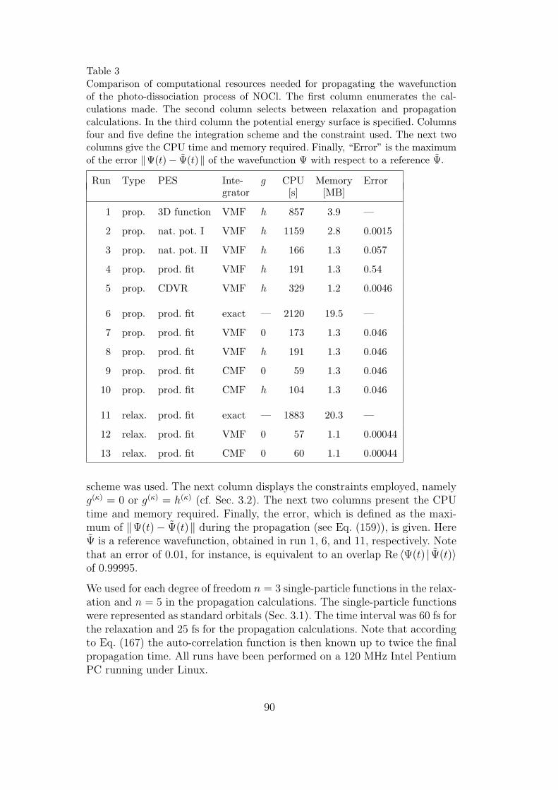
Table 3Comparison of computational resources needed for propagating the wavefunctionof the photo-dissociation process of NOCl. The first column enumerates the cal-culations made. The second column selects between relaxation and propagationcalculations. In the third column the potential energy surface is specified. Columnsfour and five define the integration scheme and the constraint used. The next twocolumns give the CPU time and memory required. Finally, “Error” is the maximumof the error ‖Ψ(t)− Ψ(t)‖ of the wavefunction Ψ with respect to a reference Ψ.

Run Type PES Inte- g CPU Memory Errorgrator [s] [MB]

1 prop. 3D function VMF h 857 3.9 —

2 prop. nat. pot. I VMF h 1159 2.8 0.0015

3 prop. nat. pot. II VMF h 166 1.3 0.057

4 prop. prod. fit VMF h 191 1.3 0.54

5 prop. CDVR VMF h 329 1.2 0.0046

6 prop. prod. fit exact — 2120 19.5 —

7 prop. prod. fit VMF 0 173 1.3 0.046

8 prop. prod. fit VMF h 191 1.3 0.046

9 prop. prod. fit CMF 0 59 1.3 0.046

10 prop. prod. fit CMF h 104 1.3 0.046

11 relax. prod. fit exact — 1883 20.3 —

12 relax. prod. fit VMF 0 57 1.1 0.00044

13 relax. prod. fit CMF 0 60 1.1 0.00044

scheme was used. The next column displays the constraints employed, namelyg(κ) = 0 or g(κ) = h(κ) (cf. Sec. 3.2). The next two columns present the CPUtime and memory required. Finally, the error, which is defined as the maxi-mum of ‖Ψ(t)− Ψ(t)‖ during the propagation (see Eq. (159)), is given. HereΨ is a reference wavefunction, obtained in run 1, 6, and 11, respectively. Notethat an error of 0.01, for instance, is equivalent to an overlap Re 〈Ψ(t) | Ψ(t)〉of 0.99995.

We used for each degree of freedom n = 3 single-particle functions in the relax-ation and n = 5 in the propagation calculations. The single-particle functionswere represented as standard orbitals (Sec. 3.1). The time interval was 60 fs forthe relaxation and 25 fs for the propagation calculations. Note that accordingto Eq. (167) the auto-correlation function is then known up to twice the finalpropagation time. All runs have been performed on a 120 MHz Intel PentiumPC running under Linux.

90

With runs 1 to 5 we want to judge the quality of the possible ways of includingthe S1 surface in an MCTDH propagation. The reference calculation, run1, where the potential matrix elements and mean-fields were determined bymulti-dimensional integration, is rather slow and requires about one third ofthe CPU time of the numerically exact calculation, run 6. This underlines theimportance of representing the potential in product form. Run 2 shows that thenatural potential expansion is able to represent the potential very accurately,however at the price that many expansion terms are needed, which slowsdown the calculation. Note that the accuracy of this potential representationis much higher than necessary for determining observable quantities, such asabsorption spectra. Due to the smallness of the system, including the potentialas a 3-dimensional function is faster than the high-accuracy natural potentialexpansion. For larger systems, however, this will not be the case.

Calculations more typical for MCTDH applications are given in runs 3 to 5. Inruns 3 and 4 the potential energy was approximated by natural potentials andthe fit of Manthe et al., respectively. Note that the number of non-separablepotential terms of the natural potential expansion is 20, and thus the sameas in the fit. The natural potential expansion is noticeable faster and at thesame time considerably more precise than the fit done “by hand”. The higheraccuracy of the natural potentials is not surprising as they are optimal in aweighted L2-sense. The error of the product fit, i.e. the norm of the differencebetween the wavefunctions of runs 1 and 4, is rather large. The spectra com-puted from these wavefunctions, however, agree reasonably well, because theauto-correlation function from which the spectra are generated is insensitiveto errors in the wavefunction that are orthogonal to Ψ(0).

In the particular case of NOCl the CDVR approach gives remarkably preciseresults, though at the price of a CPU time two times larger than with naturalpotentials. Unfortunately, we have found that this high accuracy of CDVR isgenerally not reached for other systems. (See also our comment on CDVR atthe end of Sec. 4.3.) The memory requirements were very similar for the threemethods.

Calculations 6 to 10 compare both the available integration schemes and theinfluence of the constraints. The error tolerances of the VMF and CMF inte-grators were chosen such that the integrator errors were small compared withthe MCTDH error, i.e. the convergence with respect to the single-particlefunctions. The most efficient MCTDH calculation, run 9, is 36 times faster,and needs 15 times less memory than the standard method. When employingthe constraint g(κ) = 0 the CMF scheme is about three times faster than theVMF scheme. This is a comparatively small gain, but this was to be expectedfor such a small system (In the VMF run, only 36% of the CPU time resultsfrom the computation of the mean-fields). In all MCTDH calculations thesame amount of memory was necessary.

91

It is illuminating to compare the measured gain of the CMF scheme withrespect to the standard method with the predicted gain of Eq. (92). Usingthe parameters given above, as well as an effective s = 23 (see the discussionbelow Eq. (92)), and l = 5, one obtains a gain of 111. However, NOCl is asmall system and the effort of propagating the single-particle functions is notnegligible, as assumed when deriving Eq. (92), but amounts to 73% of thetotal effort. Thus the predicted gain must be multiplied with 0.27, yielding again of 30. This value is in fact close to the measured one of 36, demonstratingthe reliability of Eq. (92).

We want to point out that it was necessary to cut large potential energy valueswhen using the standard method. This is because the potential fit of Mantheet al. shows large negative values in an unphysical region, which force theintegrator of the standard method to take small steps. Due to this, a largegain factor of 150 was reported in an earlier publication [28]. The MCTDHalgorithm, on the other hand, is less sensitive to large potential energy values.Cutting the potential thus speeds up the exact calculation and lets the gainfactor drop to the value presented here.

The influence of the constraints g(κ) = 0 and g(κ) = h(κ) in a VMF runis demonstrated in runs 7 and 8. While generally it is advantageous to setg(κ) = h(κ), since then only the residual Hamiltonian (42) is involved in thepropagation of the MCTDH coefficients, this is not the case for the NOClsystem. The reasons are that the A-vector is short (nf = 125), and that thereare merely 4 out of 26 Hamiltonian terms that are separable. On the otherhand, using the constraint g(κ) = h(κ) causes the single-particle functions tochange more rapidly, which enforces smaller integration steps. For NOCl thelatter effect dominates. In the CMF scheme, this effect is typically much moredramatic, as can be seen from runs 9 and 10. Therefore, the constraint g(κ) = 0is generally used when the CMF scheme is applied.

Our last study concerns the influence of the different integration schemes in arelaxation calculation, runs 11 to 13. A numerically exact calculation using thestandard method needs more than 30 times more CPU time, and almost 20times more memory than an MCTDH calculation. Comparing the VMF andCMF schemes, one finds that a VMF run is slightly faster. This surprising out-come is due to the smallness of the system. Since merely nf = 27 configurationsare involved, almost all computational effort is spent for the propagation ofthe single-particle functions. The error estimate of the CMF scheme, which re-quires the single-particle functions to be propagated one and a half times, thennegates all other savings. For larger systems, however, the CMF method per-forms very well in relaxation calculations, as the wavefunction soon becomesnearly converged, allowing the mean-fields to be kept constant for rather longtime steps. Reference [54] gives an example.

92

The above calculations demonstrate that even for small systems the use ofthe MCTDH scheme can lead to a considerable reduction of the computa-tional resources compared with the standard method of Sec. 2.2. The resultsalso show that the natural potential expansion offers a convenient, efficientand accurate way to incorporate the NOCl potential energy surface into anMCTDH calculation. Finally, for the example under consideration the CMFalgorithm turns out to be advantageous to the VMF integrator, even thoughthe system is small.

9.2 Reactive scattering of H+D2

The H+H2 reaction and its isotopic variants are probably the elementary re-actions most extensively studied during the last decade. They are thus oftenconsidered as typical examples of elementary bimolecular reactions, by exper-imentalists as well as by theoreticians [148,149]. From the theoretical point ofview, the resolution of this scattering problem is not as trivial as the small sizeof the system might suggest. Even thermal rate constants, which are averagedquantities, have been shown to be highly dependent on the accuracy of boththe electronic potential energy surface and the method of nuclear dynamicsused for the calculation [150–152].

Turning to MCTDH it should be noted that H3 is a rather small system. Itconsists of light atoms, and is defined by only three (internal) coordinates. Onthe other hand — like any reactive system — its motion is highly correlatedas the products are represented in the Jacobian coordinates of the reactants.Additionally, the complicated potential energy surface has to be representedin product form, requiring many expansion terms.

Hence, H+H2 reactive scattering is a problem not particularly suitable for MC-TDH. Being a small system, N and f are small, but being highly correlated,n is comparatively large. In addition to that, there is a rather large number, s,of Hamiltonian terms. (Compare with Secs. 4.4 and 5.2.6). However, as shownbelow, the H+H2 reactive scattering system has been successfully treated byMCTDH. It is thus to be expected that MCTDH will perform very efficientlywhen turning to larger reactive scattering systems, e.g. four atom systems.

In order to profit at least a little from the favourable MCTDH scaling, weshall concentrate in the following on the isotopic variant H+D2 and considertranslational energies up to the rather large value of 2.5 eV, computing cumu-lative initial-state selected cross-sections for the H+D2(ν, j)→HD+D reaction[46]. To compare with experimental results [153–155], these cross-sections arethermally averaged over a room-temperature Boltzmann distribution of theD2 rotational states. The D2 molecule is taken to be in the vibrational groundor first excited state. To our knowledge, these are the first calculations onvibrationally excited, ν=1, D2 target molecules.

93

Denoting the D–D bond distance by r, the distance from the H atom to thecentre-of-mass of the D2-molecule by R, and the angle between these axes byθ, the total Hamiltonian in the body-fixed frame within the coupled statesapproximation can be written as [64,65,156]

HJK(R, r, θ) = TR + Tr + Tθ + VLSTH(R, r, θ) +J(J+1)− 2K2

2µRR2, (212)

where

TR =− 1

2µR

∂2

∂R2, (213)

Tr =−1

2µr

∂2

∂r2, (214)

Tθ =

(1

2µRR2+

1

2µrr2

)2 , (215)

and

2 =−(

1

sin θ

∂

∂θsin θ

∂

∂θ− K2

sin2 θ

). (216)

Here µR denotes the reduced mass of the H atom and the D2-diatom, and µr

the reduced mass of the two D atoms. Within the coupled states approxima-tion not only the total angular momentum quantum number J , but also thequantum number K denoting the projection of the total angular momentumonto the body-fixed axis R are conserved, i.e. remain unchanged during thereaction process. VLSTH denotes the Liu-Siegbahn-Truhlar-Horowitz (LSTH)potential energy surface for the H3 system in its lowest electronic state [111–113].

For an efficient implementation of the MCTDH algorithm, it is necessary forthe system’s Hamiltonian to be in a product form (see Sec. 4.2). On inspectionof Eqs. (212) to (216) this is the case for the kinetic energy and centrifugalpotential terms. The LSTH potential energy surface, VLSTH(R, r, θ), can beexpanded in a product basis employing the product representation schemediscussed in Sec. 6. Instead of expanding the entire LSTH surface the interac-tion potential

V JKI (R, r, θ) = VI(R, r, θ) +

J(J + 1)− 2K2

2µRR2

≈mr∑

i=1

mθ∑

j=1

Dij(R) v(r)i (r) v

(θ)j (θ) (217)

94

was expanded in a product basis of natural potentials. The first term on theright hand side of Eq. (217) is defined as the difference between the LSTH-potential VLSTH and the potential VD2

of the free diatom D2,

VI(R, r, θ) = VLSTH(R, r, θ)− VD2(r) , (218)

which vanishes for sufficiently large values of the translational coordinate R.

In order to avoid a decrease in integrator step size due to high potentialvalues, an energy cut-off has been applied to the potential V JK

I before itwas expanded. This is the reason why the centrifugal term is included in theexpansion. To reduce the number of expansion coefficients, a contraction overthe translational degree of freedom R proved to be the most advantageous(see Eq. (121)). For the definition of the relevant regions the reader is referredto Ref. [57].

The interaction potential V JKI (Eq. (217)) was expanded for each set of quan-

tum numbers (J,K). The expansion orders were taken asmr = 12 andmθ = 9,resulting in 108 expansion coefficients. The computational effort for the de-termination of the product expansion was negligible: it took less than 2 minon an IBM RS/6000 power2 workstation to compute one expansion.

The initial wavepacket Ψ0 = Ψ(t = 0) is defined as the product of a Gaussianwavepacket χ0 (Eq. (153)), a vibrational eigenfunction ϕj0ν0 (Eq. (220)), anda L2-normalised associated Legendre polynomial PK

j0(Eq. (222)),

Ψ0(R, r, θ) = χ0(R)ϕj0ν0(r) PKj0(cos θ) . (219)

The vibrational functions are defined as the eigenfunctions,

H0,j(r)ϕjν(r) = Ejν ϕjν(r) , (220)

of the internal channel Hamiltonian corresponding to the rotational quantumnumber j,

H0,j(r) = Tr + VD2(r) +

j(j + 1)

2µrr2. (221)

The L2-normalised associated Legendre polynomials

PKj (cos θ) =

√√√√2j + 1

2

(j −K)!

(j +K)!PKj (cos θ) (222)

are eigenfunctions of the 2-operator (see Eq. (216)) with eigenvalues j(j+1).

95

The initial wavepacket, Ψ0, (if uncorrected) must be located in the asymptoticregion of the reactant channel,

(VI(R, r, θ) +

j(j + 1)

2µRR2+J(J + 1)− 2K2

2µRR2

)Ψ0(R, r, θ) ≈ 0 . (223)

This equation can always be satisfied by choosing the centre of the wavepacket,R0, large enough. However, inspection of Eq. (223) shows that the higher thetotal rotational quantum number J , the slower the centrifugal potential fallsoff, and the further away from the scattering centre the initial wavepacket hasto be placed. This results in larger grid sizes and longer propagation times.For example, for total angular momentum quantum number Jmax = 40, andvanishing quantum number K = 0, the centrifugal potential at the outer edgeof the translational grid, Rmax = 10 a.u., takes on considerable values:

Jmax(Jmax + 1)

2µRR2max

≈ 0.15 eV . (224)

Instead of placing the initial wavepacket Ψ0 far out in the asymptotic region ofthe educt channel, the adiabatic correction scheme was employed, which allowsthe initial wavepacket to be moved close to the scattering centre. The adiabaticcorrection follows the lines presented in Sec. 7.2, but only the vibrational statewas corrected adiabatically; the rotational state was treated diabatically [46].This is reasonable because the rotational motion is slow compared with thetranslational one.

Initial momentum p0 = −8.76 (−7.00) a.u. and width σR = 0.18 a.u. ofthe Gaussian wavepacket χ0 (Eq. (153)) were chosen in accordance with thedesired initial energy distribution ∆(E) (Eq. (157)). The value in bracketscorresponds to vibrationally excited H+D2(ν = 1) calculations. The initialwavepackets were placed quite close to the interaction region: the centre of thewavepacket was placed at R0 = 4.5 a.u. for the D2-molecule in its vibrationalground state, which for the vibrationally excited D2 had to be moved to R0 =5.5 a.u. to account for the larger spatial extension of the ϕj0ν=1 vibrationaleigenfunction compared with the spatial extension of the ground-state ϕj0ν=0

eigenfunction.

Without the adiabatic correction scheme it would have been necessary tolocate the initial wavepacket much further away from the scattering centre.For vanishing total angular momentum J = 0, and initial j = 0, ν = 0, a valueof R0 = 7.5 a.u. was found to be necessary [45].

For each set of quantum numbers (ν0, j0, J,K), the adiabatically corrected

96

initial wavepacket is provided in an MCTDH-compatible product basis of ap-propriately chosen single-particle functions,

Ψ0(R, r, θ) =nR−1∑

k=0

nr−1∑

ν=0

Akνj0 χk(R)ϕj0ν(r) PKj0(cos θ) . (225)

The single-particle functions of the dissociative degree of freedom χk(R) aredefined according to Eq. (154), Schmidt-orthonormalised, and are orthogonalto the Gaussian wavepacket χ0 (Eq. (153)). The ϕj0ν are vibrational eigenfunc-tions of the internal channel Hamiltonian H0,j0 (Eq. (221)), corresponding tothe initial rotational quantum number j0. The vibrational eigenfunctions ϕj0ν

for fixed rotational quantum number j0 were determined by diagonalisationof the diabatic channel Hamiltonian (Eq. (221)) represented by sine DVR (cf.App. B.4.4).

The single-particle functions of the dissociative and of the vibrational de-gree of freedom were represented on an equidistant grid by sine DVR. Thesingle-particle functions of the rotational degree of freedom were representedby symmetrised Legendre DVR, exploiting the underlying potential symmetrydue to the homonuclear diatom. Employing symmetrised Legendre DVR thenumber of grid points is halved (see App. B.4.3 for more details). The num-bers of single-particle functions used were nR = 16 (18), nr = 12 (14), andnθ = 12. Values in brackets correspond to vibrationally excited H+D2(ν = 1)calculations.

The wavepackets were propagated using the constant mean-field integrationscheme (see Sec. 5.2). The use of the constant mean-field integrator reducedthe computational effort by about an order of magnitude compared with thevariable mean-field integration scheme (see Sec. 5.1). This was accomplishedwithout a deterioration of the accuracy, and with stable self-regulation of theintegrator step size.

Initial-state selected reaction probabilities, P JKνj (E), were determined for a

broad energy range by analysing the reactive flux into the configuration chan-nel of the products. To this end the combined flux operator/complex absorbingpotential approach of Sec. 8.6 was employed.

The complex absorbing potential −iW was defined as a sum of two one-dimen-sional potentials of monomial form given by Eq. (80):

W (R, r) = WR(R) +Wr(r) . (226)

The strength parameters ηR = ηr = 0.003 a.u., the starting points Rc =6.04 (7.00) a.u. and rc = 3.24 a.u., and the orders bR = br = 3 were chosen ac-cording to the rules given in Ref. [99]. Again, the value in brackets correspondsto the vibrationally excited H+D2(ν = 1) calculation.

97

0

0.5

1

1.5

2

0.5 1 1.5 2 2.5

T=300K =0;1[ A2 ]Etrans

Fig. 3. Comparison of experimental and theoretical reaction cross-sections as a func-tion of the translational energy for the H+D2(ν = 0) and H+D2(ν = 1) reaction.The cross-sections are rotationally Boltzmann averaged for T = 300 K. The solidlines show the results of MCTDH calculations [46]. The lower curve represents theν = 0 and the upper curve the ν = 1 cross-sections. Experimental cross-sections ofBrownsword et al. [155], Levene et al. [154], and Johnston et al. [153] are depicted byfilled circles, squares, and triangles, respectively. The error-boxes and the error-barsshow the errors as given by Johnston et al. and Levene et al., respectively. Theerrors of the Brownsword et al. cross-sections are comparable to those of Johnstonet al. For reasons of clarity they are not shown. The results of rotationally averagedcoupled states calculations employing a recently developed Toeplitz approach ofCharutz et al. [157] are represented by open circles. The Charutz values are takenfrom Fig. 9 of Ref. [157]. This figure has been reprinted from Ref. [46].

The initial-state selected reaction probabilities are related to the interactionof the time evolved wavepacket Ψ(t) with the product arrangement channelCAP Wr. The energy distribution ∆(E) of the initial wavepacket determinesthe energy range for which the reaction probabilities can be computed inone step by a single propagation. To obtain room temperature rotationally-averaged reaction cross-sections σT=300K

ν=0,1 (E) for translational energies up to2.5 eV, wavepacket propagations are performed with initial quantum numbersup to jmax = 4 and Jmax = 40. As K takes values from 0 to j, 600 separatewavepacket propagations had to be performed for each initial vibrational state.

Figure 3 shows the results of MCTDH calculations [46], and compares thesewith experimental [153–155] and theoretical [157] values determined by othergroups. Depicted are rotationally averaged (T = 300 K) reaction cross-sectionsfor the H+D2(ν = 0) and H+D2(ν = 1) reaction as a function of the relativetranslational energy. The solid lines show the results of the MCTDH calcula-

98

tions. The lower curve represents the ν = 0, and the upper curve the ν = 1cross-sections.

For ν = 0, the MCTDH results are compared with the theoretical values (opencircles) of Charutz et al. [157]. The Charutz values are results of rotationallyaveraged coupled states calculations employing a Toeplitz operator approach.Charutz et al. computed reaction cross-sections for six energy values, and theMCTDH results are in excellent agreement with these data. The experimentalν = 0 values of Brownsword et al. [155], Levene et al. [154], and Johnstonet al. [153] are also depicted. Within the experimental errors there is excellentagreement between the MCTDH values and the experimental measurements.

Computational speed is of importance, since 600 independent wavepacketpropagations have to be performed for a given initial vibrational state. Eachsingle calculation is specified by a set of initial quantum numbers (ν, j, J,K).Total angular momentum values up to Jmax = 40 were necessary to obtain con-verged results in the energy range under investigation. The computational costfor a single calculation on a 400 MHz Dec-alpha workstation varies between60 and 90 minutes CPU time, depending on the initial quantum numbers.This is fast but the CPU times are comparable with those of other optimisedwavepacket propagation methods. If one takes into account that H+D2 is asmall but strongly coupled system, this fact is very encouraging. When turn-ing to larger systems we therefore expect MCTDH to perform considerablyfaster than standard wavepacket propagation. Note that the MCTDH memoryrequirements are always low. The present calculations need only 5 MB RAM.

9.3 Surface scattering of N2/LiF(001)

Several molecule-surface scattering problems have been studied using the MC-TDH method [47–53]. Here we consider the scattering of a diatom from acorrugated rigid surface. The three Cartesian coordinates (x, y, z) define theposition of the centre of mass of the molecule with the z-axis being perpen-dicular to the surface. The orientation of the diatom is described by the polarand azimuthal angles (θ, φ) with respect to the z-axis. Treating the moleculeas a rigid-rotor there are thus five degrees of freedom. The Hamiltonian reads

H = − 1

2M

(∂2

∂x2+

∂2

∂y2+

∂2

∂z2

)+Hrot(θ, φ) + V (x, y, z, θ, φ) , (227)

where

Hrot = −1

2µr2

[1

sin θ

∂

∂θsin θ

∂

∂θ+

1

sin2 θ

∂2

∂φ2

](228)

99

denotes the operator of rotational energy and where M and µ are the totaland reduced mass of the diatom, respectively.

The molecule-surface interaction potential is the surface-dumbbell model [158]

V (x, y, z, θ, φ) = 2A exp(−αz)[cosh

(αr2cos θ

)

+ β cosh(αr2cos θ

)cos

(2πxa

)cos

(πrasin θ cosφ

)

+cos(2πyb

)cos

(πrbsin θ sinφ

)

+ β sinh(αr2cos θ

)sin

(2πxa

)sin

(πrasin θ cosφ

)

+sin(2πyb

)sin

(πrbsin θ sinφ

)].

(229)

The potential parameters can be chosen to model the N2/LiF(001) interactionby taking the potential range, corrugation, internuclear distance of the rigidrotor, and lattice constants as α = 1.9012 a.u., β = 0.1, r = 2.0673 a.u.,and a = b = 5.3669 a.u., respectively. The potential strength parameter Ais arbitrary as it merely shifts the potential along the z-axis. Note that thismodel potential satisfies the MCTDH product form requirement, Eq. (64).

The angular degrees of freedom θ and φ are strongly coupled through the termsin−2 θ ∂2/∂φ2 which appears in Hrot. This coupling, in fact, becomes singularfor θ → 0 or θ → π. It thus causes numerical problems and slows down theconvergence when treated as separable. The singularity is removed by com-bining the two angular degrees of freedom (see Sec. 4.5) and representing theresulting two-mode single-particle functions by spherical harmonics Yjmj

(θ, φ).In this primitive basis Hrot is diagonal with diagonal elements j(j + 1)/2µr2.

The z-degree of freedom describes the distance from the surface and requiresrather many grid points. It is thus convenient to represent it by FFT. Themotion parallel to the surface needs to be represented only over one latticeconstant because of the periodicity of the interaction. Periodic boundary con-ditions are then required and FFT is thus the obvious choice for representingthe x and y degrees of freedom. Since these degrees of freedom require a com-paratively small number of grid points, it is of advantage to combine themand treat them as one particle (see Sec. 4.5 and 9.4). The five-dimensionalproblem is thus treated as a three particle one, two of the particles beingtwo-dimensional.

The N2/LiF(001) surface scattering problem has been investigated by the MC-TDH scheme [52], and by other methods [159,160], for scattering energies up

100

to 100 meV. We recently returned to this problem and studied it over an ex-tended energy range of 60 to 300 meV [107]. The recent technical advances,such as the correction scheme (see Sec. 7.2.2) and the use of CAPs (see Sec.4.7) combined with the flux analysis (see Sec. 8.6), allowed the z-grid lengthto be shortened by roughly a factor of three. However, because of the higherenergy the grid spacings must now be finer, making the problem much largerthan the one studied previously [52,159,160]. A converged calculation requires(Nx, Ny, Nz, Nθφ) = (24,24,108,223) grid points or primitive basis functions(jmax = 36, mj,max = 6, and taking only even j’s leads to 223 spherical har-monics as basis functions). The numbers of single-particle functions requiredare (nxy, nz, nθφ) = (35,17,70). A single wavefunction represented in the prim-itive basis needs 210 MB storage, making the standard method (see Sec. 2.2)very difficult, if not infeasible, for this problem. A MCTDH wavefunction, onthe other hand, requires merely 1.2 MB and the MCTDH calculation takesabout 15 MB, being feasible even on small computers.

For a large system like the present one with several ten thousand open states,it is no longer useful to investigate state-to-state transition probabilities. Av-eraged quantities like the average rotational energy transfer (ARET) or theaverage parallel energy transfer (APET) are often more meaningful. The fluxanalysis method is very well suited for the calculation of averaged quantities.The totally averaged rotational energy transfer is e.g. given by

ARET(E) =2

π |∆(E) |2 Re

∞∫

0

grot(τ) eiEτ dτ , (230)

where the correlation function grot is defined as

grot(τ) =

∞∫

0

dt 〈Ψ(t) |HrotW |Ψ(t+ τ)〉 (231)

(compare with Eqs. (198) to (201)). Note that the CAPW depends on z aloneand thus commutes with Hrot.

The diffraction channel-specific ARET is defined similarly by replacing grotwith gnm,rot where

gnm,rot(τ) =

∞∫

0

dt 〈Ψ(t) |PnmHrotW |Ψ(t+ τ)〉 . (232)

Here Pnm = |nm〉〈nm| is the projector on the nmth diffraction channel and

〈xy |nm〉 = (ab)−1/2 exp(2πinx/a+ 2πimy/b) (233)

101

is the nmth eigenfunction of parallel motion (normal incidence is assumed).Note that Pnm, Hrot and W mutually commute. The APET is defined analo-gously by exchanging Hrot with the expression for the parallel energy and Pnm

with the projector on a specific rotational state Pjmj. Finally, ifHrot is removed

from Eq. (232) such that only PnmW (or alternatively PjmjW ) remains, one

computes the rotationally averaged transition probability to the nmth diffrac-tion channel (or the diffraction channel averaged transition probability to thejmj rotational state). The use of the operator PnmPjmj

W eventually providesstate-to-state transition probabilities.

The totally averaged ARET shows a very simple course: ARET(E) = 0.095E.Thus 9.5% of the initial kinetic energy is transferred to rotational energy,almost independently of the kinetic energy. This finding is for the initial ro-tational state j = 0 and normal incidence. The diffraction channel averagedtransition probability to final rotational states depicts a strong rotational rain-bow structure in particular for jfinal ≥ 10 and E ≥100 meV. More details onresults may be found in [52,159] and in a forthcoming publication [107].

9.4 Photo-excitation of pyrazine

The photo-excitation of the pyrazine molecule (C4H4N2) has been extensivelyinvestigated, both experimentally and theoretically. The UV-absorption spec-trum [161,162] shows two bands close in energy. The most important featureis that while the lower energy, S1, band shows a set of discrete lines, theupper, S2, band is broad with very little structure. This lack of structure isattributed to a conical intersection between the two states, resulting in a fastradiationless transition from the upper to lower state.

For such a set of vibronically coupled states, a model Hamiltonian has beendeveloped [163]. The excited states are taken in a diabatic representation,and the Hamiltonian thus has a matrix form where the matrix indices referto the diabatic states. The diabatic potential energy surfaces, expressed inthe ground-state normal modes, are expanded in a Taylor series around theground-state equilibrium position:

H =H0 +H1 +H2 + . . . . (234)

The zeroth order expansion term is the ground-state potential energy surfaceand a term for the energy splitting between the states,

H0 =∑

i

ωi

2

(− ∂2

∂Q2i

+Q2i

)1 0

0 1

+

−∆ 0

0 ∆

, (235)

102

where ωi is the frequency of the ith normal mode with dimensionless coor-dinate Qi. The splitting between the two potential energy surfaces at theequilibrium position, Q = 0, is 2∆.

The first order terms are then linear in the normal mode coordinates, whilethe second order terms are quadratic and bi-linear,

H1 =∑

i∈G1

κ(1)i 0

0 κ(2)i

Qi +

∑

i∈G3

0 λi

λi 0

Qi , (236)

H2 =∑

(i,j)∈G2

aij 0

0 bij

QiQj +

∑

(i,j)∈G4

0 cij

cij 0

QiQj . (237)

Here, symmetry considerations play a major role. The pyrazine molecule hasthe point group D2h, and the S1 and S2 states have symmetry B3u and B2u

respectively. The first order off-diagonal coupling elements are thus non-zeroonly for modes with B1g symmetry, and the set G3 contains only the ν10a mode.The linear on-diagonal coupling elements are non-zero for vibrational modeswhich are totally symmetric, and the set G1 contains the five Ag modes: ν6a, ν1,ν9a, ν8a, and ν2. The non-zero second order coupling elements are governed bythe symmetry of products of modes. The set G4 comprises products of modeswith resulting B1g symmetry, while the set G2 products with Ag symmetry.For more details see Ref. [37].

Previous theoretical studies have shown [164,165] that the experimental spec-trum can be qualitatively reproduced when the Hamiltonian is expanded tofirst order, i.e. only coupling matrix elements linear in the normal mode coor-dinates are included. Thus only the modes in sets G1 and G3 are relevant. Ig-noring two totally symmetric modes which have very weak coupling constantsleads to a 4-mode model with the modes ν10a, ν6a, ν1, and ν9a. A phenomeno-logical broadening of the spectrum from this model is then used to accountfor the remaining 20 modes.

It thus seems reasonable to turn the problem into a system-bath interactionstudy, and replace these 20 modes by a heat bath [166]. A simple form for abath is a set of harmonic oscillators coupled linearly to the electronic states,i.e.

Hbath =nbath∑

b=1

ωb

2

(− ∂2

∂Q2b

+Q2b

)1 0

0 1

+

κ(1)b 0

0 κ(2)b

Qb , (238)

where nbath is the number of bath modes. The full Hamiltonian is then H =H0 +H1 +Hbath.

103

This is a much simpler problem than if the symmetries of the 20 less impor-tant vibrational modes are correctly taken into account. Treating the pyrazinemolecule in a more realistic manner, and expanding the Hamiltonian to sec-ond order results in a large number of terms correlating the various modes,and a much more complicated potential energy surface topology. This systemhas also been examined successfully [37], but here the simpler 4-mode systemcoupled to the bath model (238) will be used to demonstrate the applicationof the MCTDH method to a large system exhibiting a conical intersection.

The property of interest is the absorption spectrum. This can be obtainedfrom the auto-correlation function of the system (see Sec. 8.3), propagatingthe ground-state wavefunction on the excited surfaces. In this system theground state is a set of harmonic oscillators, and so the initial wavefunctionis a product of Gaussian functions.

The model Hamiltonian described above is immediately in the product formrequired for the efficient implementation of the MCTDH method, and thusit can be used without further thought. The choice of primitive DVR basisis also straightforward: the degrees of freedom are all bound oscillators, andso a harmonic oscillator DVR is the most efficient. In particular, if the DVRfunctions are generated using the ground-state normal mode frequencies andthe ground-state equilibrium position, the initial wavefunction can be exactlyrepresented.

There are three basic choices that still need to be made: the representationof the electronic basis, the choice of integrator, and how to treat such a largenumber of degrees of freedom. An idea of the optimal choices can be obtainedfrom studying the 4-mode model of pyrazine described above, i.e. includingonly significant linear coupling terms.

The first step is to find the optimal number of primitive grid points. This canbe achieved using a series of calculations, which do not need to be convergedwith respect to the number of single-particle functions. By analysing the pop-ulation at the ends of the one-dimensional grids, and monitoring changes inthe auto-correlation function, the effect of the basis size can be observed. Aprimitive basis with 22, 32, 21, and 12 grid points for the modes ν10a, ν6a, ν1,and ν9a, respectively, was found to be sufficient.

The next step is to obtain convergence with respect to the single-particlefunction basis. This was done by monitoring the auto-correlation function,using the analysis procedure described in Sec. 8.7 to show where more func-tions are required. Tab. 4 describes the memory and CPU time required forconverged MCTDH calculations, propagating the wavepacket for 120 fs usingvarious propagation methods. A calculation using the standard method withthe SIL integrator is given as a comparison.

104

Table 4Comparison of computational resources needed for the propagation of pyrazine in-cluding 4 modes. The first column enumerates the calculations made. The secondcolumn selects between the integration schemes. The label “exact” refers to thestandard method, Sec. 2.2. In the third column the type of single-particle functionbasis with respect to the electronic degree of freedom is specified (see Sec. 3.5).Column four defines whether standard, interaction picture, or natural orbitals wereused. The next two columns give the CPU time and memory required on an IBMRS/6000 power2 workstation. Finally, “Error” is the maximum error of the calcula-tion with respect to the standard method calculation, i.e. ‖ Ψ−Ψexact ‖. Note thatan error of 0.01 is equivalent to an overlap of 0.99995 (see Eq. (160)).

Run Inte- Basis Orbitals CPU Memory Errorgrator type [s] [MB]

1 exact — — 6565 67.3 —

2 VMF single-set standard 1421 6.1 0.042

3 VMF multi-set standard 820 3.0 0.034

4 VMF multi-set int. pic. 580 3.1 0.035

5 VMF multi-set natural 877 3.1 0.057

6 CMF multi-set standard 370 3.3 0.035

The required resources listed in Tab. 4 again demonstrate a large gain factorfor all MCTDH calculations with respect to the standard method calculation:the fastest calculation using the CMF integrator and multi-set formulationwas a factor of 18 times faster and required 20 times less memory. Note thatthis gain in CPU time is in good agreement with the estimated gain of 16,Eq. (92). The efficiency of the MCTDH method is especially pleasing whenone considers that the problem studied here is a system demonstrating chaoticdynamics, i.e. the wavepacket does not remain localised as in the case of thephoto-dissociation of NOCl (see Sec. 9.1). As a result, rather a large numberof single-particle functions is required.

In the single-set formulation a single-particle function basis set of (nν10a , nν6a ,nν1 , nν9a) = (16, 15, 8, 7) was required for convergence, where the notationdescribes the number of functions required for each degree of freedom re-spectively. Thus although the factor N/n is not very large the compact formof the wavefunction results in highly efficient propagation. The number ofsingle-particle functions required for the different degrees of freedom reflectsthe relative strengths of the coupling constants.

In the multi-set formulation, a basis set of (nν10a , nν6a , nν1 , nν9a) = S1(9, 15,8, 6), S2(9, 13, 7, 5) was required, where S1 and S2 denote the sets used forthe wavepackets for the respective electronic states. Comparing calculations2 and 3 shows that, despite the increase in single-particle functions required,

105

this formulation is more efficient than the single-set formulation. The reasonfor this is that by using this formulation the number of expansion coefficientshas been reduced from 26 880 to 10 575 (remember that in the single-set for-mulation there is an electronic “degree of freedom” with 2 basis functions).

On comparing calculations 3, 4, and 6 the required CPU time for the propa-gation is seen to decrease on using the more efficient interaction picture andCMF integration schemes. Calculation 5 demonstrates that there is no gain inusing the natural orbital picture over the standard single-particle functions.In fact this calculation required more time and the accuracy was lower thancalculation 3. This is due to the extra numerical inaccuracies introduced inusing the natural orbital constraints (see Eq. (56)).

The error, the maximum difference between the standard method and theMCTDH wavefunctions during the propagation, demonstrates another advan-tage of the method. The error in the MCTDH wavefunction is between 3-6%,yet the property of interest, the auto-correlation function is converged. Thuseffort is not wasted in representing unimportant parts of the wavefunction.

Having obtained a feel for the behaviour of the MCTDH method for the treat-ment of the 4-mode model, we now turn to treating a system which is impos-sible to treat using the standard method: the 4-mode system coupled to thestrongest 5 bath modes. The coupling constants are listed in Tab. 1 of Ref.[36]. The bath modes included here are numbers b1 to b5.

After some small calculations it was decided that 6 primitive basis functionsare sufficient for the bath modes. Thus, keeping the primitive basis size asbefore, a primitive basis set of (Nν10a , Nν6a , Nν1 , Nν9a , Nb1 , Nb2 , Nb3 , Nb4 ,Nb5) = (22, 32, 21, 12, 6, 6, 6, 6, 6) was used. This is a total of 1.38 × 109

functions, and a single standard method wavefunction would require 21 GBof memory.

This 9-mode system is a good demonstration of the use of combined modesto reduce the computational resources needed for large calculations (see Sec.4.5). Tab. 5 lists three calculations using different combination schemes. Againthe propagation time was 120 fs and, after the results from the 4-mode calcu-lations, the multi-set formulation was used with the CMF integration scheme.

The first is a straightforward 9-mode MCTDH calculation, i.e. no modes arecombined. The single-particle basis set is listed in the table, and despite thelarge number of expansion coefficients, 3 253 248, the calculation is feasible,although over 7 days of computer time were required. It is interesting to notethat the four pyrazine sub-system modes required fewer single-particle func-tions than in the calculations without the bath modes. This is due to the fasterrelaxation in the larger system, leading to a simplification of the dynamics.

For the second calculation a combination scheme was used in which the 4sub-system degrees of freedom were treated as two 2-dimensional particles,

106

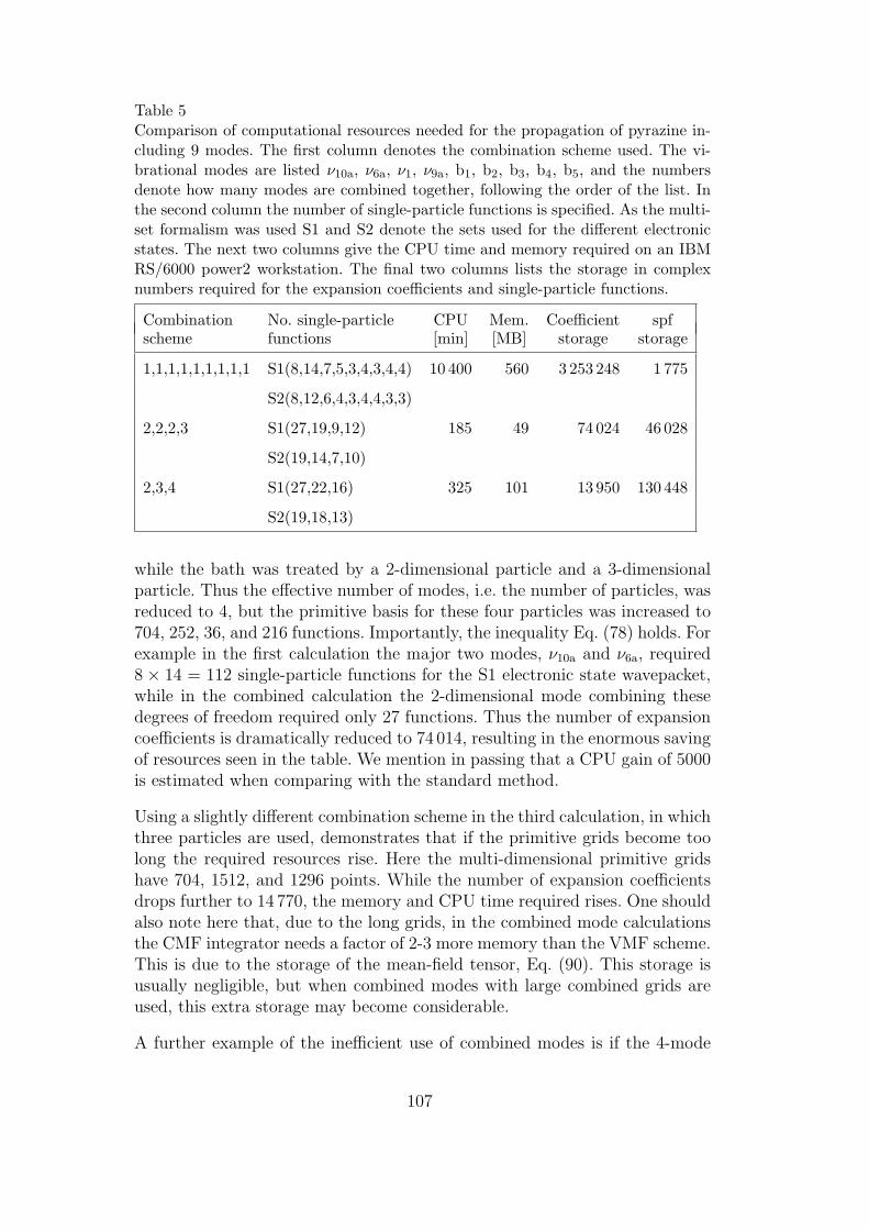
Table 5Comparison of computational resources needed for the propagation of pyrazine in-cluding 9 modes. The first column denotes the combination scheme used. The vi-brational modes are listed ν10a, ν6a, ν1, ν9a, b1, b2, b3, b4, b5, and the numbersdenote how many modes are combined together, following the order of the list. Inthe second column the number of single-particle functions is specified. As the multi-set formalism was used S1 and S2 denote the sets used for the different electronicstates. The next two columns give the CPU time and memory required on an IBMRS/6000 power2 workstation. The final two columns lists the storage in complexnumbers required for the expansion coefficients and single-particle functions.

Combination No. single-particle CPU Mem. Coefficient spfscheme functions [min] [MB] storage storage

1,1,1,1,1,1,1,1,1 S1(8,14,7,5,3,4,3,4,4) 10 400 560 3 253 248 1 775

S2(8,12,6,4,3,4,4,3,3)

2,2,2,3 S1(27,19,9,12) 185 49 74 024 46 028

S2(19,14,7,10)

2,3,4 S1(27,22,16) 325 101 13 950 130 448

S2(19,18,13)

while the bath was treated by a 2-dimensional particle and a 3-dimensionalparticle. Thus the effective number of modes, i.e. the number of particles, wasreduced to 4, but the primitive basis for these four particles was increased to704, 252, 36, and 216 functions. Importantly, the inequality Eq. (78) holds. Forexample in the first calculation the major two modes, ν10a and ν6a, required8 × 14 = 112 single-particle functions for the S1 electronic state wavepacket,while in the combined calculation the 2-dimensional mode combining thesedegrees of freedom required only 27 functions. Thus the number of expansioncoefficients is dramatically reduced to 74 014, resulting in the enormous savingof resources seen in the table. We mention in passing that a CPU gain of 5000is estimated when comparing with the standard method.

Using a slightly different combination scheme in the third calculation, in whichthree particles are used, demonstrates that if the primitive grids become toolong the required resources rise. Here the multi-dimensional primitive gridshave 704, 1512, and 1296 points. While the number of expansion coefficientsdrops further to 14 770, the memory and CPU time required rises. One shouldalso note here that, due to the long grids, in the combined mode calculationsthe CMF integrator needs a factor of 2-3 more memory than the VMF scheme.This is due to the storage of the mean-field tensor, Eq. (90). This storage isusually negligible, but when combined modes with large combined grids areused, this extra storage may become considerable.

A further example of the inefficient use of combined modes is if the 4-mode

107

model calculation is made using two 2-dimensional particles. The single-partic-le function basis required for convergence is S1(20,20), S2(15,15). Comparingthis calculation to calculation 6 in Tab. 4, the number of expansion coefficientsis reduced to 697. The memory and CPU time requirements however rise from3.3 MB and 370 seconds to 27 MB and 5480 seconds.

Thus a balance of combining degrees of freedom together to reduce the num-ber of expansion coefficients, while taking care not to produce long multi-dimensional grids for the single-particle function representations, can result inthe treatment of large systems. As a rule of thumb we note that the number ofparticles, p, should in general satisfy p ≈ d+2, or equivalently p ≈

√f + 1+1.

The power of this approach is clear, and a carefully chosen combination schemeenabled the accurate study of the full 24-dimensional pyrazine-bath problemoutlined here [36,38], as well as the realistic 24-dimensional pyrazine systemincluding linear and bi-linear coupling terms [37].

108

10 Conclusions and outlook

With the accurate treatment of the dynamics of the pyrazine molecule afterphoto-excitation (see Ref. [36–38] and Sec. 9.4), a system with 24 degrees offreedom and 2 strongly coupled, and thus highly anharmonic potential energysurfaces, it can be claimed that the MCTDH method has come of age. Thisachievement demonstrates conclusively that the method can live up to its earlypromise of being capable of treating many degrees of freedom at an affordablecost.

Since the original formulation of the MCTDH equations of motion ten yearsago, the techniques needed to implement and use the method have developed along way. Focusing on typical examples from photo-dissociation, reactive scat-tering, surface scattering, and photo-excitation, emphasis has been placed onmaking the method general, able to treat a wide range of dynamical phenom-ena. In particular, much work has been invested in using the special, extremelycompact, form of the MCTDH wavefunction.

Technical developments, such as the CMF integration scheme (see Sec. 5.2),have optimised the efficiency of the algorithm used to solve the equations ofmotion. Combined with the increase in hardware performance, this has led toa reduction in the CPU time required for the study of the photo-dissociation ofNOCl (see Sec. 9.1) from 58 minutes [28] to 8 seconds on a modern workstation.At the same time, the use of combined modes (see Sec. 4.5), has reduced thememory requirements for large systems. The automatic fitting of potentialenergy surfaces to a product form (see Sec. 6) has also enabled the efficientstudy of a variety of systems.

Looking ahead, there are still a number of possibilities that would bring fur-ther improvements to the method. The development of new DVRs will enableother types of motion, particularly rotational, to be efficiently included in acalculation. Ways of using multi-dimensional potential energy functions canalso be improved, with the CDVR method (see Sec. 4.3) providing a possiblebasis for this. For the study of large systems it is also essential to furtherreduce the memory and CPU requirements. A possible strategy is the selec-tion of important configurations. This would break the exponential growth ofthe method with the number of degrees of freedom, at the price of reducedaccuracy.

Another goal is the study of solvated systems. Here, the relevant sub-systemmay be represented by a reduced density matrix [79] and the influence of thesolvent is then accounted for by dissipative operators of the Redfield [167]or Lindblad [168] type. Such an approach requires the extension of MCTDHto density matrices [169]. An alternative route is to retain the wavefunctionpicture and account for only a finite number (10 to 30 say) of solvent atoms.

109

There are thus many solvent degrees of freedom, but the solvation dynamicsmay be very simple, so allowing an approximate, e.g. semi-classical, treatmentof the solvent dynamics. Both these extensions of the MCTDH approach arecurrently under investigation.

In conclusion, the MCTDHmethod opens up the possibility to study moleculardynamics in a general and efficient manner. It is therefore likely to play a majorrole in the theoretical study of the dynamics of molecules in the years ahead.

110

Acknowledgements

There are several people who over the years contributed to the research pre-sented here. The first one to mention is U. Manthe who wrote the very firstMCTDH program and performed the first applications as part of his PhD-thesis. We then like to thank our former post-docs M. Ehara and M.-C. Heitz,as well as A. Raab and U. V. Riss for their contributions to the MCTDHproject and for many lively discussions. Last but not least we like to thankL. S. Cederbaum for his continuous interest in and his strong support of theMCTDH project.

This work has been financially supported by the Deutsche Forschungsgemein-schaft, partly through the Schwerpunktprogramm Zeitabhangige Phanomeneund Methoden in Quantensystemen der Physik und Chemie. This support isvery gratefully acknowledged.

111

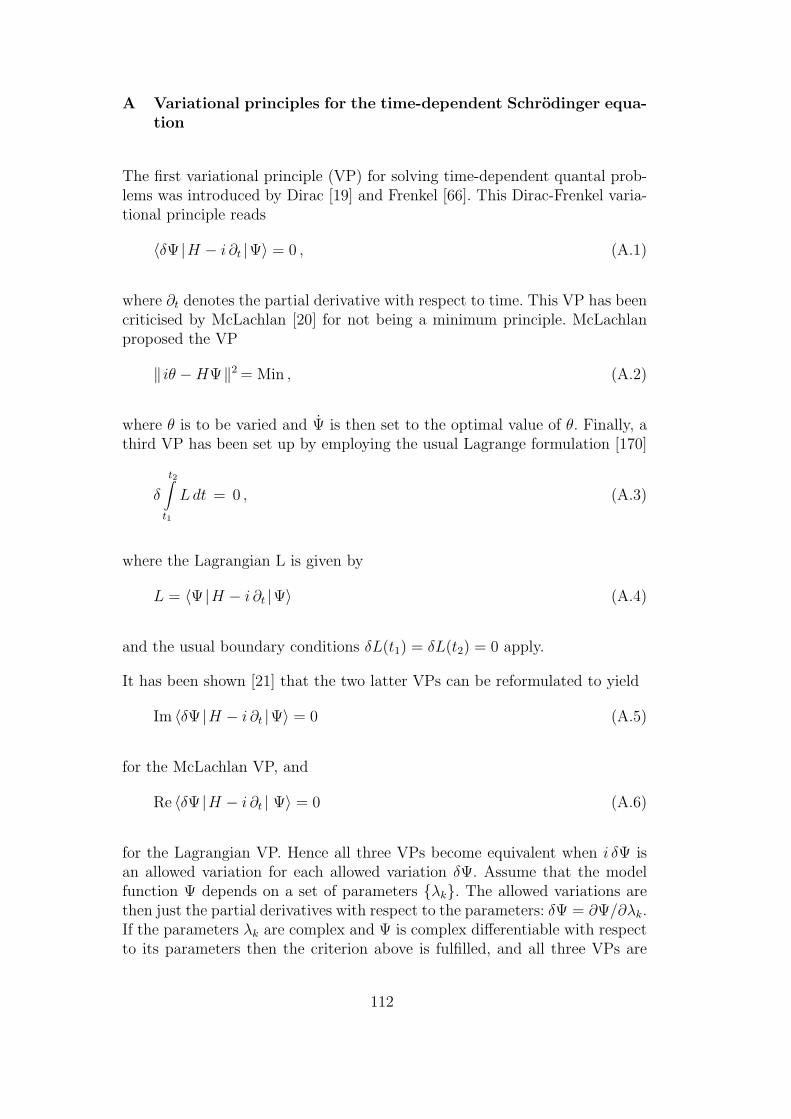
A Variational principles for the time-dependent Schrodinger equa-tion

The first variational principle (VP) for solving time-dependent quantal prob-lems was introduced by Dirac [19] and Frenkel [66]. This Dirac-Frenkel varia-tional principle reads

〈δΨ |H − i ∂t |Ψ〉 = 0 , (A.1)

where ∂t denotes the partial derivative with respect to time. This VP has beencriticised by McLachlan [20] for not being a minimum principle. McLachlanproposed the VP

‖ iθ −HΨ‖2= Min , (A.2)

where θ is to be varied and Ψ is then set to the optimal value of θ. Finally, athird VP has been set up by employing the usual Lagrange formulation [170]

δ

t2∫

t1

Ldt = 0 , (A.3)

where the Lagrangian L is given by

L = 〈Ψ |H − i ∂t |Ψ〉 (A.4)

and the usual boundary conditions δL(t1) = δL(t2) = 0 apply.

It has been shown [21] that the two latter VPs can be reformulated to yield

Im 〈δΨ |H − i ∂t |Ψ〉 = 0 (A.5)

for the McLachlan VP, and

Re 〈δΨ |H − i ∂t | Ψ〉 = 0 (A.6)

for the Lagrangian VP. Hence all three VPs become equivalent when i δΨ isan allowed variation for each allowed variation δΨ. Assume that the modelfunction Ψ depends on a set of parameters λk. The allowed variations arethen just the partial derivatives with respect to the parameters: δΨ = ∂Ψ/∂λk.If the parameters λk are complex and Ψ is complex differentiable with respectto its parameters then the criterion above is fulfilled, and all three VPs are

112

equivalent. In this case one should use the Dirac-Frenkel VP because it is thesimplest of the three.

The space of allowed variations, δΨ, is the space built by all linear com-binations of the partial derivatives ∂Ψ/∂λk where, however, only real coeffi-cients are allowed if the parameters λk are real. For later reference we notethat Ψ ∈ δΨ always holds because Ψ =

∑λk ∂Ψ/∂λk. On the other hand,

Ψ ∈ δΨ does not necessarily hold. It is true if the length of the vector Ψcan be varied, e.g. if the parameters are linear.

The parameters to be varied in case of an MCTDH model wavefunction arethe coefficients Aj1...jf and the single-particle functions ϕ

(κ)jκ . These parameters

are complex and it is sufficient to use the Dirac-Frenkel VP. The space of allallowed variations, δΨ, is thus the complex linear space

δΨ = spanΦJ ,Ψ

(κ)lκχ(κ)

, (A.7)

where “span” denotes the complex linear space spanned by the arguments.Ψ

(κ)lκ

denotes a single-hole function as defined in Sec. 3.1, χ(κ) denotes anarbitrary square-integrable function and the indices J , κ and lκ run over theirusual sets. Ψ ∈ δΨ holds for MCTDH wavefunctions because Ψ =

∑AJ ΦJ .

TheoremThe equations of motion derived from the Dirac-Frenkel variational princi-ple conserve both norm and energy, if the Hamiltonian is explicitly time-independent, ∂tH = 0, and if the model wavefunction Ψ itself is containedin the space of the allowed variations: Ψ ∈ δΨ.

In order to prove this theorem, first an expression for the time derivative ofthe expectation value of the nth moment of the Hamiltonian is derived:

d

dt〈Ψ |Hn |Ψ〉= 〈Ψ |Hn |Ψ〉+ 〈Ψ |Hn |Ψ〉

=2Re 〈Ψ |Hn |Ψ〉=−2 Im 〈HnΨ |−i ∂t |Ψ〉=−2 Im 〈HnΨ |H − i ∂t |Ψ〉 . (A.8)

The transformation of the last line was performed by addition of the realexpectation value 〈Ψ |Hn+1 |Ψ〉.

For n = 0 Eq. (A.8) proves the conservation of norm:

d

dt〈Ψ |1 |Ψ〉 = −2 Im 〈Ψ |H − i ∂t |Ψ〉 = 0 , (A.9)

113

as Eq. (A.1) ensures that 〈Ψ | H − i ∂t | Ψ〉 vanishes because δΨ = Ψ is anallowed variation by assumption.

The case n = 1 demonstrates the conservation of energy:

d

dt〈Ψ |H |Ψ〉=−2 Im 〈HΨ |H − i ∂t |Ψ〉

=−2 Im[〈(H − i ∂t)Ψ |(H − i ∂t)Ψ〉+ 〈i ∂tΨ |H − i ∂t |Ψ〉

]

=2Re 〈∂tΨ |H − i ∂t |Ψ〉=0 , (A.10)

since δΨ = ∂tΨ is always an allowed variation (see above).

Finally, n = 2 yields the energy deviation:

d

dt〈Ψ |H2 |Ψ〉=−2 Im 〈H2Ψ |H − i ∂t |Ψ〉

=−2 Im[〈(H − i ∂t)Ψ |H |(H − i ∂t)Ψ〉 (A.11)

+ 〈i ∂tΨ |H (H − i ∂t) |Ψ〉]

=−2 Im 〈i ∂tΨ |H (H − i ∂t) |Ψ〉=2Re 〈H ∂tΨ |H − i ∂t |Ψ〉6=0 in general , (A.12)

since, in general, δΨ = H ∂tΨ is not an allowed variation.

114

B Discrete variable representation (DVR)

The discrete variable representation (DVR) is a powerful method for rep-resenting wavefunctions and operators. It is a general approach which is ofinterest on its own and is only loosely connected to MCTDH. We thereforefind it convenient to adopt here a notation that is well suited for the followingdiscussion, but is slightly different from the one used elsewhere in this review.The coordinate is now called x (rather than Q), and ϕ denotes a basis functionwhich must not be confused with a single-particle function. To clearly distin-guish operators from their matrix representation and eigenvalues, we indicatean operator by a hat (ˆ), and mark vectors and matrices by bold face type.

B.1 VBR and FBR representation of the potential

We consider a one-dimensional problem and choose a complete square-inte-grable basis set

ϕj(x)∞j=1 , (B.1)

where xϕj(x) and ϕ′j(x) = dϕj/dx are also square-integrable. It is further

assumed that the matrix elements

Qjk = 〈ϕj | x |ϕk〉 (B.2)

D(1)jk = 〈ϕj |d/dx |ϕk〉 (B.3)

D(2)jk = 〈ϕj |d2/dx2 |ϕk〉 (B.4)

can be evaluated analytically. We truncate the basis set to its first N members,ϕj(x)Nj=1, and introduce the projector onto the finite basis set,

P =N∑

j=1

|ϕj〉〈ϕj | , (B.5)

as well as the N×N matrices Q,D(1) andD(2), the matrix elements of whichare given by Eqs. (B.2), (B.3), and (B.4).

As a result, as the matrices D(1) and D(2) are known, there is no problem inevaluating the kinetic energy when computing matrix elements of the Hamil-tonian H = T + V . The evaluation of matrix elements of the potential,

V VBRjk = 〈ϕj | V |ϕk〉 , (B.6)

115

is however in general non-trivial. In fact, the computation of these matrixelements by accurate numerical integration may take considerable more com-putational time than the full diagonalisation of the Hamilton matrix. Thesuperscript VBR appearing in the above equation stands for variational basis-set representation. This naming [85] emphasises that the eigenvalues of thethus obtained Hamiltonian matrix are variational upper bounds to the exactones.

The potential operator V can be considered as a real function V of the positionoperator x, i.e. V = V (x). Turning from operators to their matrix represen-tation one may consider the potential matrix as a function of the positionmatrix Q, i.e.

V FBR = V (Q) , (B.7)

where the superscript FBR stands for finite basis-set representation.

Equation (B.7) would be exact (i.e. V FBR would equal V VBR) if the basisset were complete. Since we are using a truncated basis set, however, we areintroducing an error. This can be most easily seen by considering the quadraticpotential V (x) = x2. Then

V VBR = P V P = P x2P (B.8)

and

V FBR = V(P xP

)= P xP xP . (B.9)

However, Eq. (B.7) is a useful approximation. To evaluate it one diagonalisesQ,

Q = UXU † , (B.10)

where U denotes the eigenvector matrix and X is the diagonal matrix ofeigenvalues xα, i.e. Xαβ = xα δαβ. (Note that we are numbering the basisfunctions by Latin letters j, k, . . . and the grid points, xα, by Greek lettersα, β, . . .) The potential matrix elements in the finite basis-set representationare then given by

V FBRjk =

N∑

α=1

Ujα V (xα)U∗kα . (B.11)

This idea of evaluating potential matrix elements by diagonalisation of theposition operator goes back to Harris et al. [83].

116

It is instructive to investigate the relationship between Eq. (B.11) and aquadrature formula,

V quadjk =

N∑

α=1

wα ϕ∗j(xα)V (xα)ϕk(xα) , (B.12)

where wα are the weights of the quadrature. Equating V FBR with V quad yields

w1/2α = U∗

kα/ϕk(xα) , (B.13)

which implies that U∗kα/ϕk(xα) must be independent of k, but there is no rea-

son why this should hold in general. However, for tridiagonal representationsof the position operator Dickinson and Certain [84] were able to show thatthe FBR representation (B.7) and (B.11) is equivalent to a Gaussian quadra-ture. Provided Q is tridiagonal for all N , Eq. (B.13) holds and its right handside is independent of k. Moreover, the Gaussian quality (see Sec. B.3) of thequadrature ensures that the overlap integrals as well as the matrix elementsof the position operator are then given exactly by quadrature:

N∑

α=1

wα ϕ∗j(xα)ϕk(xα)= 〈ϕj |ϕk〉 = δjk , (B.14)

N∑

α=1

wα ϕ∗j(xα) xα ϕk(xα)= 〈ϕj | x |ϕk〉 = Qjk . (B.15)

One therefore expects that the FBR is more accurate when using basis func-tions ϕj that tridiagonalise x, e.g. harmonic oscillator functions.

B.2 Diagonalisation DVR

We have introduced the FBR approach in order to efficiently (but approxi-mately) evaluate potential matrix elements. To this end the eigenvalues xα andthe eigenvector matrix U of the position operator were needed. The knowl-edge of the unitary matrix U allows us to perform a conceptually new step:the matrix U is used to unitarily transform the FBR to the discrete variablerepresentation (DVR). To this end we establish the DVR functions

χα(x) =N∑

j=1

ϕj(x)Ujα . (B.16)

117

These functions are orthonormal, 〈χα |χβ〉 = δαβ, and diagonalise — by con-struction — the position operator 〈χα | x |χβ〉 = xα δαβ. From the last equationfollows:

x χα(x) = xα χα(x) + rα(x) , (B.17)

where the residual term rα is orthogonal to the basis, i.e. P rα = 0. If rαvanished, χα would necessarily be proportional to δ(x − xα). Hence χα actslike a δ-function within the space spanned by the basis set.

Next we transform the Hamiltonian, i.e. the kinetic energy T and the potentialV , to the DVR:

TDVR =U † T U , (B.18)

V DVR =U † V FBRU , (B.19)

with Tjk = 〈ϕj | T |ϕk〉. Note that TDVRαβ = 〈χα | T |χβ〉 is an exact expression,

while V DVRαβ = 〈χα | V | χβ〉 holds only approximately because the FBR ap-

proximation has been adopted. Using Eqs. (B.11) and (B.19) one immediatelyfinds that

V DVRαβ = V (xα) δαβ . (B.20)

It is this relation what makes the DVR so attractive.

It has been discussed in the previous section that the FBR approximation isrelated to a Gaussian quadrature if the representation of the position operatoris tridiagonal. If the DVR is based on such an FBR we will speak of a properDVR, and of an improper DVR if the matrix Q is not tridiagonal. In thefollowing we shall concentrate on proper DVRs, but note that the CDVRmethod of Sec. 4.3 is based on an improper DVR.

For a proper DVR it is not difficult to prove that the following results hold:discrete orthonormality,

N∑

α=1

wα ϕ∗j(xα)ϕk(xα) = δjk , (B.21)

discrete completeness,

N∑

j=1

(wαwβ)1/2 ϕ∗

j(xα)ϕj(xβ) = δαβ , (B.22)

118

discrete δ-property,

χα(xβ) = w−1/2α δαβ (B.23)

and

〈χα |ψ〉 = w1/2α ψ(xα) , (B.24)

where the last equation is only valid if ψ lies entirely in the basis set, i.e.Pψ = ψ. Equation (B.24) turns a (proper) DVR into a collocation method.The wavefunction is no longer represented by its overlaps with basis functions,but by its values on grid points xα, i.e.

ψ(x)→ ψ =(w

1/21 ψ(x1), w

1/22 ψ(x2), . . . , w

1/2N ψ(xN)

)T. (B.25)

As a final remark we note that it is sometimes advantageous not to diagonalisethe position operator x but some real, invertable function of it, ˆx = g(x).Such a change of variables may be necessary in order to arrive at a tridiagonalrepresentation (see Secs. B.4.2, B.4.3, B.4.4 and B.4.5). The grid points arethen given by xα = g−1(xα), where the xα are the eigenvalues of the matrixrepresentation of ˆx.

B.3 Quadrature DVR

A (proper) DVR may be alternatively derived from a Gaussian quadrature,circumventing the diagonalisation of the position operator. This route wasfollowed by Light and coworkers [85,86,171,172], who coined the abbreviationsVBR, FBR and DVR.

Assume that there are a non-negative weight function w(x) and polynomi-als pj(x), (j = 0, 1, . . .) of degree j, which are orthogonal to each otherwith respect to the weight function w(x). (For example, the Hermite poly-nomials are orthogonal to each other with respect to the weight functionw(x) = exp(−x2).) Then there exists a Gaussian quadrature formula [102]with weights wα and nodes xα such that

∫w(x) f(x) dx =

N∑

α=1

wα f(xα) (B.26)

holds exactly for all polynomials of degree lower or equal to 2N − 1.

119

Next one defines the basis functions ϕj as

ϕj(x) = Aj w1/2(x) pj−1(x) , j = 1, . . . , N , (B.27)

where Aj is a normalisation constant. This is an orthonormal basis set byconstruction. Because the Gaussian quadrature rule (B.26) is exact for allpolynomials up to (2N − 1)th degree, one finds that all overlap integrals andall matrix elements of the position operator are exactly reproduced by thequadrature formula, i.e. Eqs. (B.14) and (B.15) hold.

Following Light et al. [85] we introduce a transformation matrix

Yαj = w1/2α ϕj(xα) (B.28)

and find that this matrix is unitary,

(Y † Y

)jk

=N∑

α=1

wα ϕ∗j(xα)ϕk(xα) = δjk . (B.29)

The unitarity of Y implies that(Y Y †

)αβ

= δαβ also holds, which — when

inserting Eq. (B.28) — proves discrete completeness, Eq. (B.22). Introducingthe DVR functions

χα(x) =N∑

j=1

Y ∗αj ϕj(x) =

N∑

j=1

w1/2α ϕ∗

j(xα)ϕj(x) , (B.30)

it is easy to show that these functions satisfy the δ-property, Eqs. (B.23) and(B.24). (Set x = xβ in the last equation and use discrete completeness.) Allpotential matrix elements are evaluated by the Gaussian quadrature rule. Thisand the δ-property leads to the DVR formula (B.20) for the potential.

Finally, when comparing Eq. (B.13) with Eq. (B.28), one finds that Y = U †

holds, showing that a quadrature DVR and a (proper) diagonalisation DVRare equivalent. (There is no improper quadrature DVR.) As discussed in theprevious section it may be advantageous to transform the variable x to x =g(x), because there may be a Gaussian quadrature rule only when integratingover the new variable x. See Secs. B.4.2, B.4.3, B.4.4, and B.4.5 for examples.

B.4 Examples

In the following sections some particular DVRs and related representationswill be discussed.

120

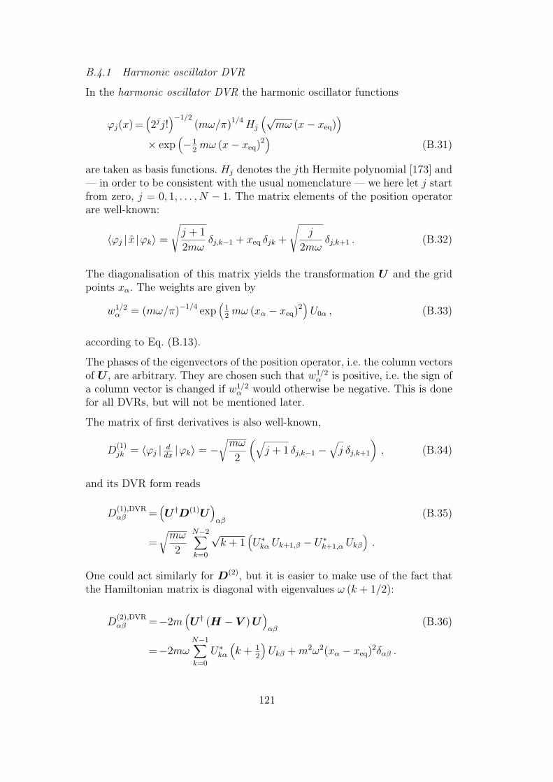
B.4.1 Harmonic oscillator DVR

In the harmonic oscillator DVR the harmonic oscillator functions

ϕj(x)=(2jj!

)−1/2(mω/π)1/4Hj

(√mω (x− xeq)

)

× exp(−1

2mω (x− xeq)2

)(B.31)

are taken as basis functions. Hj denotes the jth Hermite polynomial [173] and— in order to be consistent with the usual nomenclature — we here let j startfrom zero, j = 0, 1, . . . , N − 1. The matrix elements of the position operatorare well-known:

〈ϕj | x |ϕk〉 =√j + 1

2mωδj,k−1 + xeq δjk +

√j

2mωδj,k+1 . (B.32)

The diagonalisation of this matrix yields the transformation U and the gridpoints xα. The weights are given by

w1/2α = (mω/π)−1/4 exp

(12mω (xα − xeq)2

)U0α , (B.33)

according to Eq. (B.13).

The phases of the eigenvectors of the position operator, i.e. the column vectorsof U , are arbitrary. They are chosen such that w1/2

α is positive, i.e. the sign ofa column vector is changed if w1/2

α would otherwise be negative. This is donefor all DVRs, but will not be mentioned later.

The matrix of first derivatives is also well-known,

D(1)jk = 〈ϕj | d

dx|ϕk〉 = −

√mω

2

(√j + 1 δj,k−1 −

√j δj,k+1

), (B.34)

and its DVR form reads

D(1),DVRαβ =

(U †D(1)U

)αβ

(B.35)

=

√mω

2

N−2∑

k=0

√k + 1

(U∗kα Uk+1,β − U∗

k+1,α Ukβ

).

One could act similarly for D(2), but it is easier to make use of the fact thatthe Hamiltonian matrix is diagonal with eigenvalues ω (k + 1/2):

D(2),DVRαβ =−2m

(U † (H − V )U

)αβ

(B.36)

=−2mωN−1∑

k=0

U∗kα

(k + 1

2

)Ukβ +m2ω2(xα − xeq)2δαβ .

121

B.4.2 Radial harmonic oscillator DVR

The radial harmonic oscillator DVR is an appropriate DVR when the wave-function is defined on a half-axis [x0,∞[ only, and satisfies the boundary con-dition ψ(x0) = 0. The odd harmonic oscillator functions are chosen as basis:

ϕj(x) =√2ϕHO

2j−1(x) , (B.37)

where j = 1, . . . , N , and where ϕHO denotes a harmonic oscillator functionas defined by Eq. (B.31), but with xeq replaced by x0 for convenience. Thenormalisation factor

√2 appears because one now considers only a half-axis.

The position operator does not have a tridiagonal representation in this basis,but the transformed variable z = (x− x0)2 does:

Qjk = 〈ϕj | z |ϕk〉 , (B.38)

=

√2j (2j + 1)

2mωδj,k−1 +

4j − 1

2mωδj,k +

√(2j − 1)(2j − 2)

2mωδj,k+1 .

The DVR grid points and weights are obtained after diagonalisation of thismatrix:

xα =√zα + x0 (B.39)

w1/2α = π1/4 (mω)−3/4 (x− x0)−1 exp

(12mω (xα − xeq)2

)U1α , (B.40)

where zα denotes an eigenvalue of the (transformed) position operator matrix(B.38).

The matrix elements of d/dx are not analytically given in the radial harmonicoscillator basis, one uses the operator 1

2((x− x0) d/dx+ d/dx (x− x0)) in-

stead. This first derivative operator has the matrix elements

D(1)jk =

1

2〈ϕj |(x− x0)

d

dx+

d

dx(x− x0) |ϕk〉

=−√2j (2j + 1) δj,k−1 +

√(2j − 1)(2j − 2) δj,k+1 . (B.41)

The matrix of second derivatives, D(2), has matrix elements similar to Eq.(B.38), but with negative off-diagonal elements and with 1/(mω) replaced bymω. The transformation of the derivative matrices to DVR form is similarto Eqs. (B.35) and (B.36) but with

√mω/2

√k + 1 replaced by

√2k (2k + 1),

and with (k + 1/2) replaced by (2k − 1/2), respectively. The sums run nowfrom 1 to N .

122

B.4.3 Legendre DVR

A Legendre DVR is employed for angular degrees of freedom because the as-sociated Legendre functions Pm

l (cos θ) are eigenfunctions of the angular mo-mentum operator

l2 = − 1

sin θ

d

dθsin θ

d

dθ+

m2

sin2 θ, (B.42)

where the magnetic quantum number m is treated as a fixed parameter. Thebasis functions are thus the L2-normalised associated Legendre functions,

ϕl−m+1(θ) = Pml (θ) = (−1)m

√√√√2 l + 1

2

(l −m)!

(l +m)!Pml (cos θ) , (B.43)

with m ≥ 0 and l restricted to m ≤ l ≤ m + N − 1. These functions areclosely related to the spherical harmonics: Ylm(θ, φ) = (2π)−1/2Pm

l (cos θ) eimφ

for m ≥ 0.

From the recurrence relation of the Legendre polynomials [173] follows therecursion

cl+1Pml+1(x)− xPm

l (x) + clPml−1(x) = 0 , (B.44)

with

cl =

√l2 −m2

4 l2 − 1(B.45)

and

x = cos θ . (B.46)

It is now obvious that in the present case one should not diagonalise the matrixrepresentation of the coordinate θ — this would not lead to a tridiagonalmatrix — but diagonalise the representation of the transformed coordinatex = cos θ. The matrix representation of x follows directly from Eq. (B.44)since the polynomials Pm

l are orthonormal.

In the case of a Legendre DVR it is convenient to replace the derivative oper-ator d/dθ by d/dθ sin θ. (Multiplying the latter operator with the imaginary

123

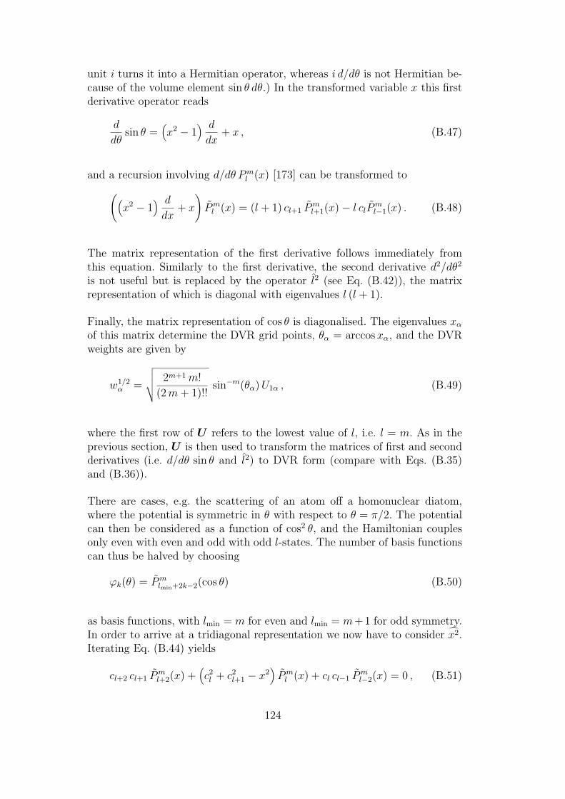
unit i turns it into a Hermitian operator, whereas i d/dθ is not Hermitian be-cause of the volume element sin θ dθ.) In the transformed variable x this firstderivative operator reads

d

dθsin θ =

(x2 − 1

) d

dx+ x , (B.47)

and a recursion involving d/dθ Pml (x) [173] can be transformed to

((x2 − 1

) d

dx+ x

)Pml (x) = (l + 1) cl+1 P

ml+1(x)− l clPm

l−1(x) . (B.48)

The matrix representation of the first derivative follows immediately fromthis equation. Similarly to the first derivative, the second derivative d2/dθ2

is not useful but is replaced by the operator l2 (see Eq. (B.42)), the matrixrepresentation of which is diagonal with eigenvalues l (l + 1).

Finally, the matrix representation of cos θ is diagonalised. The eigenvalues xαof this matrix determine the DVR grid points, θα = arccos xα, and the DVRweights are given by

w1/2α =

√√√√ 2m+1m!

(2m+ 1)!!sin−m(θα)U1α , (B.49)

where the first row of U refers to the lowest value of l, i.e. l = m. As in theprevious section, U is then used to transform the matrices of first and secondderivatives (i.e. d/dθ sin θ and l2) to DVR form (compare with Eqs. (B.35)and (B.36)).

There are cases, e.g. the scattering of an atom off a homonuclear diatom,where the potential is symmetric in θ with respect to θ = π/2. The potentialcan then be considered as a function of cos2 θ, and the Hamiltonian couplesonly even with even and odd with odd l-states. The number of basis functionscan thus be halved by choosing

ϕk(θ) = Pmlmin+2k−2(cos θ) (B.50)

as basis functions, with lmin = m for even and lmin = m+1 for odd symmetry.In order to arrive at a tridiagonal representation we now have to consider x2.Iterating Eq. (B.44) yields

cl+2 cl+1 Pml+2(x) +

(c2l + c2l+1 − x2

)Pml (x) + cl cl−1 P

ml−2(x) = 0 , (B.51)

124

which shows that the matrix representation of x2 is tridiagonal. The resultingeigenvalues are called x2α, and the grid points θα = arccos(xα) lie in the interval]0, π/2[, whereas they are distributed over ]− π/2, π/2[ when no symmetry isused.

The expression (B.49) for the weights remains unchanged for even symmetry(lmin = m), but is to be replaced by

w1/2α =

√√√√ 2m+1m!

(2m+ 3)!!(cos θα sinm θα)

−1 U1α (B.52)

for odd symmetry (lmin = m+ 1). As the first derivative we now define

1

2

(d

dθsin θ cos θ + cos θ

d

dθsin θ

)=

3x2 − 1

2+ x

(x2 − 1

) d

dx, (B.53)

the matrix elements of which can be deduced from the recursion

(3x2 − 1

2+ x

(x2 − 1

) d

dx

)Pml (x) = (B.54)

(l +

3

2

)cl+1 cl+2 P

ml+2(x)−

(l − 1

2

)cl cl−1 P

ml−2(x) .

Otherwise the procedure remains unchanged.

B.4.4 Sine DVR

The sine DVR uses the particle-in-a-box eigenfunctions as a basis. The boxboundaries are x0 and xN+1, and L = xN+1 − x0 denotes the length of thebox. The basis functions are thus

ϕj(x) =

√2Lsin (jπ(x− x0)/L) for x0 ≤ x ≤ xN+1

0 else. (B.55)

The derivative matrices are very simple:

D(1)jk = 〈ϕj |

d

dx|ϕk〉 = mod(j − k, 2) 4

L

jk

j2 − k2 , j 6= k , (B.56)

D(2)jk = 〈ϕj |

d2

dx2|ϕk〉 = −δjk (jπ/L)2 , (B.57)

125

where mod(j − k, 2) is zero if j − k is even, and one otherwise. D(1)jk vanishes

for j = k.

The matrix representation of the position operator x, however, is not tridiag-onal. To arrive at a tridiagonal form the transformed variable

z = cos (π(x− x0)/L) (B.58)

is introduced. The position operator matrix then reads

Qjk = 〈ϕj | z |ϕk〉 =1

2(δj,k+1 + δj,k−1) . (B.59)

This matrix is particularly simple and — in fact — can be diagonalised ana-lytically! The eigenvectors and eigenvalues of Q are

Ujα =

√2

N + 1sin

(jαπ

N + 1

)(B.60)

and

zα = cos(

απ

N + 1

). (B.61)

This leads to the DVR grid points

xα = x0 +L

πarccos(zα) = x0 + α

L

N + 1= x0 + α∆x . (B.62)

The grid is thus equidistantly spaced with the spacing ∆x = L/(N + 1). Itnow becomes clear why the box boundaries have been called x0 and xN+1.Note that these points do not belong to the grid; the wavefunction vanishesthere by construction.

An evenly spaced grid should lead to constant weights, and indeed one finds

w1/2α = Ujα/ϕj(xα) =

√∆x . (B.63)

The transformation of the first derivative matrix to DVR form is done numer-ically,

D(1),DVRαβ =

N∑

j,k=1

U∗jαD

(1)jk Ukβ , (B.64)

126

but the transformation of the second derivative matrix can be done analyti-cally:

D(2),DVRαβ = −

(π∆x

)2

13+ 1

6 (N+1)2− 1

2 (N+1)2 sin2( απN+1)

, α = β

2 (−1)α−β

(N+1)2sin( απ

N+1) sin(βπ

N+1)(cos( απ

N+1)−cos( βπ

N+1))2 , α 6= β

. (B.65)

Some final remarks are appropriate. The basis functions (B.55) may be writtenas (2/L)1/2 sin (j arccos(z)). This shows that they are related to the Chebyshevpolynomials of the second kind [173]. The sine DVR is therefore also known asChebyshev DVR. The sine DVR has recently been discussed by Colbert andMiller [174] who generalised it (by introducing an additional approximation)to arrive at a “universal” DVR.

B.4.5 Exponential DVR

The exponential DVR is equivalent to FFT. It is our experience that theexponential DVR performs faster than FFT for small grids (N <

∼ 16), butFFT is considerably faster for large grids (N >

∼ 100). Since the exponentialDVR is, on the one hand, rather well-documented in the literature [174–176]and, on the other hand, similar to the sine DVR, we will discuss it here onlybriefly.

When deriving the exponential DVR it is convenient to concentrate on an oddnumber of basis functions. We hence set N = 2n + 1 and let the index j runbetween −n and n rather than 1 and N . The basis functions are written as

ϕj(x) = L−1/2 exp (2iπj(x− x0)/L) , −n ≤ j ≤ n . (B.66)

They are obviously periodic,

ϕj(x) = ϕj(x+ L) , (B.67)

but we consider ϕj as being defined only on the interval [x0, xN ] with L = xN−x0. The wavefunctions to be represented satisfy periodic boundary conditions,ψ(x0) = ψ(xN).

As in the sine DVR one has to use the transformed variable z = cos(π(x −x0)/L) in order to arrive at a tridiagonal representation of the (transformed)position operator. This matrix is again given by Eq. (B.59). All subsequentmanipulations can be done analytically, yielding

127

∆x=L/N , (B.68)

xα = x0 + α∆x , (B.69)

wα =∆x . (B.70)

The derivative matrices read

D(1),DVRαβ =

0 , if α = βπ

L(−1)α−β 1

sin (π(α− β)/N), if α 6= β

, (B.71)

D(2),DVRαβ =

− π2

3L2(N2 − 1) , if α = β

−2π2

L2(−1)α−β cos (π(α− β)/N)

sin2 (π(α− β)/N), if α 6= β

. (B.72)

B.4.6 Spherical harmonics FBR

The spherical harmonics FBR is the appropriate choice when there is rota-tional motion which must be described by two angles, θ and φ. The sphericalharmonics Yjm(θ, φ) serve as basis functions. The matrix elements of the angu-lar momentum operators j2, j+, j−, and jz are then given by simple formulas.These are well-discussed in textbooks [177,178] and need not to be reportedhere. The potential matrix elements

Vjmj′m′ = 〈Yjm |V (θ, φ) |Yj′m′〉 (B.73)

can be evaluated by Gauss quadrature. The θ-nodes and -weights are takento be those of the Legendre DVR for m = 0, and the φ-nodes and -weightsare taken to be those of the exponential DVR. In the actual calculationswe usually take more nodes than there are basis functions, which makes therepresentation more VBR like.

B.4.7 Fast Fourier transform (FFT)

The Fast Fourier transform (FFT) method may be considered as an exponen-tial DVR where, however, the derivative matrices are not built but the actionof them on the wavefunction is evaluated by two FFTs. The FFT method iswell-documented in the literature [7,82,179], and there is no need to discussit here any further. We only remark that we use a Temperton FFT [180–182]which allows us to use grids the length of which can be factorised into powersof 2, 3, and 5, i.e.

N = 2j3k5l , (B.74)

where j, k, l are non-negative integers. This gives us sufficient flexibility whenchoosing the grid length.

128

C The Lanczos and the Lanczos-Arnoldi integrator

In this appendix we briefly review the short iterative Lanczos (SIL) integrationscheme [63], and discuss two different error estimates for the SIL method. Areliable error estimate and step size control for the SIL integrator is importantfor the efficiency of the CMF scheme detailed in Sec. 5.2. We consider here thecomplex Lanczos, or Lanczos-Arnoldi, algorithm [103–105], since it includesthe Hermitian Lanczos as a special case.

In the Lanczos scheme the exact Hamiltonian H is approximated by the re-duced Hamiltonian HL = PLHPL, where PL denotes the projector on theKrylov space spanned by the set of vectorsHkψ(t), k = 0, . . . , L. The Lanczos-Arnoldi recursion,

χ(0)j+1=Hψj (C.1)

for i = 0, . . . , j : χ(i+1)j+1 =χ

(i)j+1 − βijψi with βij = 〈ψi |χ(i)

j+1〉ψj+1=χ

(j+1)j+1 /βj+1,j with βj+1,j = ‖χ(j+1)

j+1 ‖ ,

constructs an orthonormal basis ψ0, . . . , ψL, starting from a normalised stateψ0, in which the reduced Hamiltonian HL is a complex upper Hessenbergmatrix:

〈ψj |HL |ψk〉 =

βjk for j ≤ k + 1

0 else, j, k = 0, . . . , L . (C.2)

(If H is Hermitian, then matrix (C.2) becomes symmetric, i.e. tridiagonal.)The Lanczos-Arnoldi algorithm requires L+ 1 evaluations of H |ψ〉.

The SIL integrator approximates the propagated wavefunction ψ(t+ τ) by

|ψ(t+ τ)〉 = e−iHLτ |ψ(t)〉 =L∑

k=0

a(L)k |ψk〉 (C.3)

with

a(L)k =

L∑

j=0

Tkj e−iλjτ

(T−1

)j0

(C.4)

and ψ0 = ψ(t)/‖ψ(t)‖. The λj specify the eigenvalues and T the eigenvectormatrix of the small, and hence easy to diagonalise, upper Hessenberg matrix(C.2).

129

The Lanczos recurrence in its standard form is in so far inefficient as thevector ψL+1 as well as the matrix element βL+1,L are determined but neverused. A slight modification of the SIL algorithm can circumvent this. As hasbeen suggested by Manthe et al. [183] one may increase the SIL order toL′ = L+ 1 by adding a further, approximate, column to the Lanczos matrix.To this end we set βL′L′ = βLL, βL,L′ = βL′,L, and βj,L′ = 0 for j < L. Theupper Hessenberg matrix is then an L′×L′ matrix, and the summation in Eqs.(C.3) and (C.4) extends to L′ rather than L. The wavefunction propagatedwith this modified algorithm is correct up to an order τL

′

, while it is onlyaccurate up to an order τL in the conventional Lanczos scheme.

For the conventional SIL integrator there exists a very convenient estimate forthe difference ∆ψ of the propagated and the exact wavefunction [63], namely

‖∆ψ‖≈ β10 . . . βL+1,L

(L+ 1)!τL+1 , (C.5)

which may be used to adjust either the step size τ or the order L. For themodified SIL integrator one could use the same formula but replace L by L′.However, βL′+1,L′ is unknown, and instead of estimating it we prefer to useEq. (C.5) as it is. Since for any one-step method, such as Lanczos, the orderof the global discretisation error is a power one lower than that of the localerror [101], the error estimate therefore controls the global rather than thelocal error.

Turning again to the conventional Lanczos integrator we note that the errorestimate (C.5) is correct to an order of L+ 1, yet the true error also containscontributions from higher orders of τ . These contributions depend not onlyon the sub-diagonal but on all elements of matrix (C.2). Despite these highercontributions, the error formula (C.5) is remarkably accurate for small stepsizes. However, it may grossly overestimate the error when the integrator isrunning at high order and thus taking large step sizes [54].

A more reliable error estimate for the (modified) Lanczos integrator is givenby [54]

‖∆ψ‖ = ‖a(L′) − a(L′−1) ‖ , (C.6)

where a zero is appended to the shorter of the two vectors, a(L′−1). Thiscriterion thus takes as an error estimate the norm of the difference betweenthe wavefunctions propagated by the SIL method of order L′ and L′ − 1. Theaccuracy of the propagation can be controlled by increasing the SIL orderL′ until the predicted error (C.6) becomes smaller than the prescribed errortolerance.

130

The improved error estimate is predominantly determined by the error of thesolution obtained with an order of L′− 1. Hence the propagated wavefunctionis one order in τ more accurate than the error estimate indicates. This is verymuch in the spirit of what has been discussed above, namely using Eq. (C.5)for the modified Lanczos integrator as well. Equation (C.6) seems to be rathercostly because it requires the diagonalisation of matrix (C.2) after each SILiteration. However, for large systems the evaluation of H |ψ〉 needs so muchnumerical effort that the effort for the error estimation remains negligible. Forlarge step sizes the improved error measure (C.6) estimates the SIL integrationerror more accurately than the standard estimate (C.5), while for small stepsizes both estimates are equally accurate [54].

131

D L2-error of the product representation

In the following the L2-error of the potential representation (see Eq. (95))

V appI =

m∑

J

CJ vIJ (D.1)

is determined, and an estimation of the error is given. Here I = (i1, . . . , if )is a multi-index. The upper summation index m denotes the set of potentialexpansion orders mκ, vIJ =

∏fκ=1 viκjκ denotes a configuration of natural

potentials, and the multi-index I represents all product grid points. If foreach degree of freedom the potential expansion orders, mκ, and the numberof product grid points, Nκ, are equal, then the potential representation isexact:

VI =N∑

J

CJ vIJ . (D.2)

Having introduced this nomenclature, the L2-error (see Eq. (99)) can be de-termined:

∆2≡N1∑

i1=1

. . .Nf∑

if=1

(Vi1...if − V app

i1...if

)2

=N∑

I

[(N∑

L

CLvILN∑

M

CMvIM

)

︸ ︷︷ ︸V 2I

+

(m∑

L

CLvILm∑

M

CMvIM

)

︸ ︷︷ ︸(V app

I)2

−(

N∑

L

CLvILm∑

M

CMvIM

)−(

m∑

L

CLvILN∑

M

CMvIM

)]

=N∑

I

[V 2I + (V app

I )2]− 2

N∑

L

m∑

M

CLCM

N∑

I

vILvIM

︸ ︷︷ ︸δLM︸ ︷︷ ︸∑

I(V app

I)2

=N1∑

i1=1

. . .Nf∑

if=1

[(Vi1...if

)2 −(V appi1...if

)2]

=N1∑

i1=1

. . .Nf∑

if=1

∣∣∣Ci1...if

∣∣∣2 −

m1∑

j1=1

. . .mf∑

jf=1

∣∣∣Cj1...jf

∣∣∣2

(D.3)

=N1∑

j1=m1+1

N2∑

j2=1

. . .Nf∑

jf=1

∣∣∣Cj1...jf

∣∣∣2+

m1∑

j1=1

N2∑

j2=m2+1

N3∑

j3=1

. . .Nf∑

jf=1

∣∣∣Cj1...jf

∣∣∣2+

132

. . .+m1∑

j1=1

. . .mf−1∑

jf−1=1

Nf∑

jf=mf+1

∣∣∣Cj1...jf

∣∣∣2. (D.4)

The last transformation can be proven by induction. Introducing the notation

aκ =mκ∑

iκ=1

and bκ =Nκ∑

iκ=mκ+1

, i.e. aκ + bκ =Nκ∑

iκ=1

, (D.5)

the summation over all indices may be alternatively written as

N1∑

i1=1

. . .Nf∑

if=1

=f∏

κ=1

(aκ + bκ) . (D.6)

Adding the second term of Eq. (D.3) to the equations (D.3) and (D.4), theinduction hypothesis in the new nomenclature reads

f∏

κ=1

(aκ + bκ) = (D.7)

b1 (a2 + b2) (a3 + b3) · · · (af−1 + bf−1) (af + bf )

+ a1 b2 (a3 + b3) · · · (af−1 + bf−1) (af + bf )

+ a1 a2 b3 · · · (af−1 + bf−1) (af + bf )...

+ a1 a2 a3 · · · af−1 bf

+ a1 a2 a3 · · · af−1 af

f + 1

summation

terms .

For f = 1 the induction hypothesis is obviously satisfied

1∏

κ=1

(aκ + bκ) = b1 + a1 .

Performing one induction step one obtains the induction hypothesis for f + 1

f+1∏

κ=1

(aκ + bκ) =

f∏

κ=1

(aκ + bκ)

(af+1 + bf+1) (D.8)

133

=

b1 (a2 + b2) (a3 + b3) · · · (af + bf ) (af+1 + bf+1)

+ a1 b2 (a3 + b3) · · · (af + bf ) (af+1 + bf+1)

+ a1 a2 b3 · · · (af + bf ) (af+1 + bf+1)...

+ a1 a2 a3 · · · af bf+1

+ a1 a2 a3 · · · af af+1

f + 2

summation

terms ,

proving the validity of the induction hypothesis.

Having determined the L2-error of the product expansion (D.4) as a functionof the expansion coefficients Cj1...jf , an error estimation as a function of the

natural populations λ(κ)jκ is derived as follows.

The potential density matrices (κ), defined according to Eq. (94), are diago-

nal in the basis of their eigenvectors, the natural potentials v(κ)jκ , and can be

expressed in terms of the potential expansion coefficients Cj1...jf as follows:

diag,(κ)αβ =

N1∑

j1=1

. . .Nκ−1∑

jκ−1=1

Nκ+1∑

jκ+1=1

. . .Nf∑

jf=1

Cj1...α...jfCj1...β...jf = δαβλ(κ)α . (D.9)

Thus, the natural populations λ(κ)jκ define an upper limit for the square of the

modulus of the potential expansion coefficients,

|Cj1...jf |2≤ minλ(1)j1 , . . . , λ

(f)jf

. (D.10)

Comparing this inequality with the L2-error of the product expansion (D.4)shows that the potential expansion can be safely truncated if the correspondingnatural populations are sufficiently small.

134

E Overview of software packages

In this appendix the MCTDH program package will be briefly described. Theprograms are written mainly in standard Fortran 77. Particular care hasbeen taken to make the program user friendly, both with respect to usageand development. The structure is modular, with information being passedbetween the modules using read-write files and common blocks contained ininclude files. Documentation is in Html format.

The package has been implemented on a number of different platforms, andApp. E.6 gives some information on the installation of the code. This set ofprograms will be made available on request to the authors.

E.1 The MCTDH program

The MCTDH program creates an initial wavepacket and propagates it in time,i.e. it solves the MCTDH equations of motion (see Sec. 3.1). The program con-tains four sequential sections which reflect the stages of the calculation: prim-itive basis (DVR) generation; representation of the operator in the primitivebasis; generation of the initial wavefunction; propagation of the wavefunction.

Desired options and input parameters can be comfortably specified in an inputfile with the aid of keywords and arguments. If a parameter is not specified areasonable default is taken. Conversion factors are built in, so that data canbe input in a variety of units.

For the primitive basis functions, the FFT and DVR schemes of App. B areavailable.

The Hamiltonian is specified in a text file which is translated by the program.The program is capable of parsing a variety of mathematical expressions, whichoften allows the Hamiltonian to be implemented in terms of an analytic for-mula, avoiding the need to write a routine for that purpose. More complicatedfunctions can be added to the library of functions. If a potential does nothave an analytic product form (64), one can use the natural potential fit (Sec.6.1), determined by the Potfit program (see below). Alternatively, the multi-dimensional potential can be used with the CDVR method (Sec. 4.3). Complexabsorbing potentials (Sec. 4.7) may also be included in the Hamiltonian.

The initial wavepacket can be set up by employing the methods described inSec. 7. Multi-mode single-particle functions, recommended for large systemsor for strongly coupled degrees of freedom (Sec. 4.5), can be simply defined.Non-adiabatic systems can be treated within both the single- and the multi-setformulation (Sec. 3.5).

135

The wavepacket may be propagated using the VMF or the CMF integrationscheme (Sec. 5). In addition to the standard single-particle functions, theprogram allows the use of natural (Sec. 3.3) and interaction picture (Sec. 3.4)orbitals. The program can also be used to propagate wavepackets employingthe standard or the TDH method (Sec. 2.2 and 2.3).

E.2 The Potfit program

The Potfit program comprises all the features presented in Sec. 6. Havinggiven the potential energy values of an arbitrarily chosen surface on a productgrid, the potential energy surface is expanded in a set of natural potentials.The input parameters (e.g. the set of expansion orders mκ, the contractionmode, the energy cut-off, the number of iteration steps) are specified in thesame manner as the MCTDH input parameters, i.e. using keywords in aninput file. The product grid points can be generated employing the same FFTand DVR schemes used for the representation of the single-particle functionsof the subsequent MCTDH calculation. The potential data generated can thenbe used directly by the MCTDH program.

E.3 The Analyse programs

The Analyse suite of programs serves to extract observable quantities fromthe data produced during the propagation, e.g. the wavefunction or auto-correlation function. In principle there is a library of routines to read andextract data from the files produced by the MCTDH program. The variousAnalyse programs then manipulate this data to extract the quantity of inter-est. The library of routines thus provides an interface to the MCTDH program,easing the development of new Analyse programs.

The programs enable one, for example, to determine and display photo-ab-sorption and photo-dissociation spectra (see Sec. 8.3), reaction probabilities(Sec. 8.6), state populations (Sec. 8.5), and adiabatically corrected energydistributions (Sec. 7.2).

Programs also exist to check the accuracy of a calculation. The convergence ofa calculation with respect to the number of single-particle functions can be ex-amined by computing the natural populations (Sec. 3.3), estimating the errorof the auto-correlation function (Sec. 8.7), or comparing two wavefunctionswith different numbers of single-particle functions (Sec. 8.2). One may alsodetect numerical inaccuracies by checking the orthonormality of the single-particle functions, or the conservation of the norm of the wavefunction. Fi-nally, the step-sizes of the VMF and CMF integration scheme (Sec. 5) can beanalysed.

136

Standard plot programs, such as GnuPlot or Xmgr, can then be used tovisualise these results. TheMathematica program, driven by script files, canalso be used to automatically produce graphical output from the programs.This is particularly useful for animation graphics, such as the evolution of thedensity along a coordinate with time.

E.4 The Filter program

With the aid of the Filter program one may determine ro-vibrational spectraof molecules or clusters using the filter-diagonalisation method (see Sec. 8.4).A Mathematica routine for plotting the obtained line spectrum also exists.Different damping functions, variational principles, and error estimates areavailable (see Ref. [126] for details). As in the MCTDH program, the input isbased on keywords.

E.5 The MCTDH library

In the above-mentioned programs a variety of standard mathematical prob-lems have to be solved. We have stored the corresponding routines in a librarywhich can also be used independently of the MCTDH package. The librarycontains efficient routines for many operations involving vectors, matrices andtensors (multiplication, inversion, etc.), solvers for several kinds of linear equa-tions and eigenvalue problems, fast Fourier transformation, spline interpola-tion, and string manipulation. Furthermore, the library includes a number ofintegrators for ordinary differential equations, such as an Adams-Bashforth-Moulton predictor-corrector, a Bulirsch-Stoer extrapolation scheme, a shortiterative Lanczos and Lanczos-Arnoldi method, and a second-order differenc-ing integrator.

E.6 System requirements

Our MCTDH software package has been installed on a variety of platforms,ranging from personal computers through various workstations to large vectormachines. Tab. E.1 offers an overview of the platforms on which our code hasrun so far. The compilation of the program is very easy: a shell-script recog-nises the architecture being used and automatically chooses the appropriatecompiler options and settings. The system requirements are quite small. Forthe automatic compilation a C-shell is needed, as well as a Posix-make. A fewroutines are written in C and require an Ansi-C compiler. An Html browser(e.g. Netscape) is needed for reading the program documentation. In orderto visualise the results computed with the Analyse programs (see App. E.3),

137

Table E.1The platforms on which our MCTDH software package has been installed so far.The first two columns specify the machine type. In the third column the operatingsystem is given. The fourth column denotes the compiler that has been used.

Machine Architecture Operating Compilersystem

CRAY J90 Unicos f90

T90

DEC alpha Ultrix f77

HP 9000/755 HP UX fort77

IBM powerPC AIX xlf

power

power2

PC pentium Linux g77

SGI mips2 Irix f77

Sun sparc20 SunOS f77

Mathematica is recommended. Note that no commercial libraries, such asImsl, Essl or Nag, are necessary. On all machines listed in Tab. E.1, withthe exception of CRAY, shared libraries are supported.

138

References

[1] Time-dependent methods for quantum dynamics, edited by K. C. Kulander(Elsevier, Amsterdam, 1991).

[2] R. Schinke, Photodissociation Dynamics (Cambridge University Press,Cambridge, 1993).

[3] Dynamics of Molecules and Chemical Reactions, edited by R. E. Wyatt andJ. Z. H. Zhang (Marcel Dekker, New York, 1996).

[4] M. Manz and L. Woste, Femtosecond Chemistry (Wiley-VCH, Weinheim,1994).

[5] Femtochemistry, edited by M. Chergui (World Scientific, Singapore, 1996).

[6] R. B. Gerber, R. Kosloff, and M. Berman, Computer Phys. Rep. 5, 59 (1986).

[7] R. Kosloff, J. Phys. Chem. 92, 2087 (1988).

[8] Numerical Grid Methods and their Application to Schrodinger’s Equation,edited by C. Cerjan (Kluwer Academic Publishers, Dordrecht, 1993).

[9] C. Leforestier, R. H. Bisseling, C. Cerjan, M. D. Feit, R. Friesner, A.Guldenberg, A. Hammerich, G. Jolicard, W. Karrlein, H.-D. Meyer, N. Lipkin,O. Roncero, and R. Kosloff, J. Comp. Phys. 94, 59 (1991).

[10] R. Kosloff, Ann. Rev. Phys. Chem. 45, 145 (1994).

[11] Z. Bacic and J. C. Light, J. Chem. Phys. 85, 4594 (1986).

[12] Z. Bacic and J. C. Light, J. Chem. Phys. 86, 3065 (1987).

[13] S. Liu, Z. Bacic, J. W. Moskowitz, and K. E. Schmidt, J. Chem. Phys. 103,1829 (1995).

[14] M. Warken and V. Bonacic-Koutecky, Chem. Phys. Lett. 272, 284 (1997).

[15] R. E. Wyatt, C. Iung, and C. Leforestier, J. Chem. Phys. 97, 3458 (1992).

[16] M. L. Brewer, J. S. Hulme, and D. E. Manolopoulos, J. Chem. Phys. 106,4832 (1997).

[17] M. F. Hermann, Ann. Rev. Phys. Chem. 45, 83 (1994).

[18] M. A. Sepulveda and F. Grossmann, Adv. Chem. Phys. 96, 191 (1996).

[19] P. A. M. Dirac, Proc. Cambridge Philos. Soc. 26, 376 (1930).

[20] A. D. McLachlan, Mol. Phys. 8, 39 (1964).

[21] J. Kucar, H.-D. Meyer, and L. Cederbaum, Chem. Phys. Lett. 140, 525 (1987).

[22] H.-D. Meyer, J. Kucar, and L. Cederbaum, J. Math. Phys. 29, 1417 (1988).

139

[23] J. Kucar and H.-D. Meyer, Z. Phys. D 18, 325 (1991).

[24] N. Makri and W. H. Miller, J. Chem. Phys. 87, 5781 (1987).

[25] R. Kosloff, A. D. Hammerich, and M. A. Ratner, in Large finite systems:

Proceedings of the twentieth Jerusalem Symposium of Quantum Chemistry and

Biochemistry, edited by J. Jortner and B. Pullman (Reidel, Dordrecht, 1987).

[26] A. D. Hammerich, R. Kosloff, and M. A. Ratner, Chem. Phys. Lett. 171, 97(1990).

[27] H.-D. Meyer, U. Manthe, and L. S. Cederbaum, Chem. Phys. Lett. 165, 73(1990).

[28] U. Manthe, H.-D. Meyer, and L. S. Cederbaum, J. Chem. Phys. 97, 3199(1992).

[29] H.-D. Meyer, U. Manthe, and L. S. Cederbaum, in Numerical Grid Methods

and their Application to Schrodinger’s Equation, edited by C. Cerjan (KluwerAcademic Publishers, Dordrecht, 1993), pp. 141–152.

[30] H.-D. Meyer, in The Encyclopedia of Computational Chemistry, edited by P.v. R. Schleyer, N. L. Allinger, T. Clark, J. Gasteiger, P. A. Kollman, H. F.Schaefer III, and P. R. Schreiner (John Wiley and Sons, Chichester, 1998),pp. 3011–3018.

[31] U. Manthe, H.-D. Meyer, and L. S. Cederbaum, J. Chem. Phys. 97, 9062(1992).

[32] U. Manthe and A. D. Hammerich, Chem. Phys. Lett. 211, 7 (1993).

[33] A. D. Hammerich, U. Manthe, R. Kosloff, H.-D. Meyer, and L. S. Cederbaum,J. Chem. Phys. 101, 5623 (1994).

[34] L. Liu, J.-Y. Fang, and H. Guo, J. Chem. Phys. 102, 2404 (1995).

[35] G. Worth, H.-D. Meyer, and L. S. Cederbaum, J. Chem. Phys. 105, 4412(1996).

[36] G. Worth, H.-D. Meyer, and L. S. Cederbaum, J. Chem. Phys. 109, 3518(1998).

[37] A. Raab, G. Worth, H.-D. Meyer, and L. S. Cederbaum, J. Chem. Phys. 110,936 (1999).

[38] G. Worth, H.-D. Meyer, and L. S. Cederbaum, Chem. Phys. Lett. 299, 451(1999).

[39] J.-Y. Fang and H. Guo, J. Chem. Phys. 102, 1944 (1995).

[40] A. Jackle and H.-D. Meyer, J. Chem. Phys. 102, 5605 (1995).

[41] U. Manthe and F. Matzkies, Chem. Phys. Lett. 252, 71 (1996).

[42] F. Matzkies and U. Manthe, J. Chem. Phys. 106, 2646 (1997).

140

[43] F. Matzkies and U. Manthe, J. Chem. Phys. 108, 4828 (1998).

[44] F. Matzkies and U. Manthe, J. Chem. Phys. 110, 88 (1999).

[45] A. Jackle and H.-D. Meyer, J. Chem. Phys. 109, 2614 (1998).

[46] A. Jackle, M.-C. Heitz, and H.-D. Meyer, J. Chem. Phys. 110, 241 (1999).

[47] A. P. J. Jansen, J. Chem. Phys. 99, 4055 (1993).

[48] J.-Y. Fang and H. Guo, J. Chem. Phys. 101, 5831 (1994).

[49] J.-Y. Fang and H. Guo, Chem. Phys. Lett. 235, 341 (1995).

[50] A. P. J. Jansen and H. Burghgraef, Surf. Sci. 344, 149 (1995).

[51] A. Capellini and A. P. J. Jansen, J. Chem. Phys. 104, 3366 (1996).

[52] M. Ehara, H.-D. Meyer, and L. S. Cederbaum, J. Chem. Phys. 105, 8865(1996).

[53] R. Milot and A. P. J. Jansen, J. Chem. Phys. 109, 1966 (1998).

[54] M. H. Beck and H.-D. Meyer, Z. Phys. D 42, 113 (1997).

[55] U. Manthe, J. Chem. Phys. 105, 6989 (1996).

[56] A. Jackle and H.-D. Meyer, J. Chem. Phys. 104, 7974 (1996).

[57] A. Jackle and H.-D. Meyer, J. Chem. Phys. 109, 3772 (1998).

[58] E. J. Heller, J. Chem. Phys. 62, 1544 (1975).

[59] M. D. Feit, J. A. Fleck Jr., and A. Steiger, J. Comp. Phys. 47, 412 (1982).

[60] M. D. Feit and J. A. Fleck Jr., J. Chem. Phys. 78, 301 (1983).

[61] M. D. Feit and J. A. Fleck Jr., J. Chem. Phys. 80, 2578 (1984).

[62] H. Tal-Ezer and R. Kosloff, J. Chem. Phys. 81, 3967 (1984).

[63] T. J. Park and J. C. Light, J. Chem. Phys. 85, 5870 (1986).

[64] P. McGuire and D. J. Kouri, J. Chem. Phys. 60, 2488 (1974).

[65] R. T. Pack, J. Chem. Phys. 60, 633 (1974).

[66] J. Frenkel, Wave Mechanics (Clarendon Press, Oxford, 1934).

[67] P. Jungwirth and R. B. Gerber, J. Chem. Phys. 102, 6046 (1995).

[68] P. Jungwirth and R. B. Gerber, J. Chem. Phys. 102, 8855 (1995).

[69] P. Jungwirth, E. Fredj, and R. B. Gerber, J. Chem. Phys. 104, 9332 (1996).

[70] Modern Methods for Multidimensional Dynamics Computations in Chemistry,edited by R. B. Gerber, P. Jungwirth, E. Fredj, A. Rom, and D. L. Thompson(World Scientific, Singapore, 1998).

141

[71] R. D. Coalson, Chem. Phys. Lett. 165, 443 (1990).

[72] J. Campos-Martinez and R. D. Coalson, J. Chem. Phys. 93, 4740 (1990).

[73] J. Campos-Martinez and R. D. Coalson, J. Chem. Phys. 99, 9629 (1993).

[74] J. R. Waldeck, J. Campos-Martinez, and R. D. Coalson, J. Chem. Phys. 94,2773 (1991).

[75] E. Camona-Novillo, D. Calloto, and J. Campos-Martinez, J. Chem. Phys. 104,8016 (1996).

[76] P. Jungwirth and B. Schmidt, Chem. Phys. Lett. 275, 127 (1997).

[77] P. Jungwirth, E. Fredj, and R. B. Gerber, J. Chem. Phys. 107, 8963 (1997).

[78] R. McWeeny, Methods of Molecular Quantum Mechanics (Academic Press,London, 1989).

[79] K. Blum, Density matrix theory and applications (Plenum Press, New York,1981).

[80] U. Manthe, J. Chem. Phys. 101, 2652 (1994).

[81] A. Jackle, Ph.D. thesis, Universitat Heidelberg, 1997.

[82] D. Kosloff and R. Kosloff, J. Comp. Phys. 52, 35 (1983).

[83] D. O. Harris, G. G. Engerholm, and G. W. Gwinn, J. Chem. Phys. 43, 1515(1965).

[84] A. S. Dickinson and P. R. Certain, J. Chem. Phys. 49, 4209 (1968).

[85] J. C. Light, I. P. Hamilton, and J. V. Lill, J. Chem. Phys. 82, 1400 (1985).

[86] J. C. Light, in Time-Dependent Quantum Molecular Dynamics, edited by J.Broeckhove and L. Lathouwers (Plenum, New York, 1992), pp. 185–199.

[87] E. Sim and N. Makri, J. Chem. Phys. 102, 5616 (1995).

[88] C. Leforestier and R. E. Wyatt, J. Chem. Phys. 78, 2334 (1983).

[89] R. Kosloff and D. Kosloff, J. Comp. Phys. 63, 363 (1986).

[90] G. Jolicard and E. Austin, Chem. Phys. Lett. 121, 106 (1985).

[91] G. Jolicard, C. Leforestier, and E. Austin, J. Chem. Phys. 88, 1026 (1988).

[92] U. V. Riss and H.-D. Meyer, J. Phys. B 26, 4503 (1993).

[93] D. Neuhauser and M. Baer, J. Chem. Phys. 90, 4351 (1989).

[94] D. Neuhauser and M. Baer, J. Chem. Phys. 91, 4651 (1989).

[95] I. Last, A. Baram, H. Szichman, and M. Baer, J. Phys. Chem. 97, 7040 (1993).

[96] T. Seideman and W. H. Miller, J. Chem. Phys. 96, 4412 (1992).

142

[97] T. Seideman and W. H. Miller, J. Chem. Phys. 97, 2499 (1992).

[98] U. V. Riss and H.-D. Meyer, J. Phys. B 28, 1475 (1995).

[99] U. V. Riss and H.-D. Meyer, J. Chem. Phys. 105, 1409 (1996).

[100] A. Vibok and G. G. Balint-Kurti, J. Chem. Phys. 96, 7615 (1992).

[101] C. W. Gear, Numerical Initial Value Problems in Ordinary Differential

Equations (Prentice-Hall, Englewood Cliffs, New Jersey, 1971).

[102] W. H. Press, S. A. Teukolsky, W. T. Vetterling, and B. P. Flannery, Numerical

Recipes (Cambridge University Press, Cambridge, 1992).

[103] W. E. Arnoldi, Q. Appl. Math. 9, 17 (1951).

[104] Y. Saad, Lin. Alg. Appl. 34, 269 (1980).

[105] R. A. Friesner, L. S. Tuckerman, B. C. Dornblaser, and T. V. Russo, J. Sci.Comp. 4, 327 (1989).

[106] M. H. Beck and H.-D. Meyer, unpublished results.

[107] M.-C. Heitz and H.-D. Meyer, unpublished results.

[108] E. Schmidt, Math. Ann. 63, 433 (1906).

[109] A. Jackle and H.-D. Meyer, J. Chem. Phys. 105, 6778 (1996).

[110] R. Schinke, M. Nonella, H. U. Suter, and J. R. Huber, J. Chem. Phys. 93,1098 (1990).

[111] P. Siegbahn and B. Liu, J. Chem. Phys. 68, 2457 (1978).

[112] D. G. Truhlar and C. J. Horowitz, J. Chem. Phys. 68, 2466 (1978).

[113] D. G. Truhlar and C. J. Horowitz, J. Chem. Phys. 71, 1514 (1979).

[114] J. Z. H. Zhang, D. J. Kouri, K. Haug, D. W. Schwenke, Y. Shima, and D. G.Truhlar, J. Chem. Phys. 88, 2492 (1988).

[115] R. Kosloff and H. Tal-Ezer, Chem. Phys. Lett. 127, 223 (1986).

[116] D. J. Tannor and D. E. Weeks, J. Chem. Phys. 98, 3884 (1993).

[117] D. E. Weeks and D. J. Tannor, Chem. Phys. Lett. 207, 301 (1993).

[118] U. Manthe, Ph.D. thesis, Universitat Heidelberg, 1991.

[119] V. Engel, Chem. Phys. Lett. 189, 76 (1992).

[120] D. Neuhauser, J. Chem. Phys. 93, 2611 (1990).

[121] M. R. Wall and D. Neuhauser, J. Chem. Phys. 102, 8011 (1995).

[122] V. A. Mandelshtam and H. S. Taylor, J. Chem. Phys. 107, 6756 (1997).

143

[123] T. P. Grozdanov, V. A. Mandelshtam, and H. S. Taylor, J. Chem. Phys. 103,7990 (1995).

[124] V. A. Mandelshtam, T. P. Grozdanov, and H. S. Taylor, J. Chem. Phys. 103,10074 (1995).

[125] G.-J. Kroes, M. R. Wall, J. W. Pang, and D. Neuhauser, J. Chem. Phys. 106,1800 (1997).

[126] M. H. Beck and H.-D. Meyer, J. Chem. Phys. 109, 3730 (1998).

[127] E. Narevicius, D. Neuhauser, H. J. Korsch, and N. Moiseyev, Chem. Phys.Lett. 276, 250 (1997).

[128] V. A. Mandelshtam, J. Chem. Phys. 108, 9999 (1998).

[129] K. C. Kulander and E. J. Heller, J. Chem. Phys. 69, 2439 (1978).

[130] R. C. Mowrey and D. J. Kouri, J. Chem. Phys. 84, 6466 (1986).

[131] Y. Sun, R. C. Mowrey, and D. J. Kouri, J. Chem. Phys. 87, 339 (1987).

[132] D. Neuhauser, J. Chem. Phys. 93, 7836 (1990).

[133] G. G. Balint-Kurti, R. N. Dixon, and C. C. Marston, J. Chem. Soc., FaradayTrans. 86, 1741 (1990).

[134] G. G. Balint-Kurti, R. N. Dixon, C. C. Marston, and A. J. Mulholland,Computer Phys. Comm. 63, 126 (1991).

[135] D. E. Weeks and D. J. Tannor, Chem. Phys. Lett. 224, 451 (1994).

[136] W. H. Miller, S. D. Schwartz, and J. W. Tromp, J. Chem. Phys. 79, 4889(1983).

[137] W. H. Thompson and W. H. Miller, Chem. Phys. Lett. 206, 123 (1993).

[138] D. Neuhauser and M. Baer, J. Phys. Chem. 94, 185 (1990).

[139] D. Neuhauser, M. Baer, R. S. Judson, and D. J. Kouri, J. Chem. Phys. 93,312 (1990).

[140] D. E. Manolopoulos and M. H. Alexander, J. Chem. Phys. 97, 2527 (1992).

[141] D. H. Zhang, Q. Wu, and J. Z. H. Zhang, J. Chem. Phys. 102, 124 (1995).

[142] N. Balakrishnan and N. Sathyamurthy, Chem. Phys. Lett. 240, 119 (1995).

[143] T. Peng, D. H. Zhang, J. Z. H. Zhang, and R. Schinke, Chem. Phys. Lett. 248,37 (1996).

[144] D. Neuhauser, M. Baer, R. S. Judson, and D. J. Kouri, Computer Phys. Comm.63, 460 (1991).

[145] J.-Y. Fang and H. Guo, J. Mol. Struct. (Theochem) 341, 201 (1995).

144

[146] T. Gerdts and U. Manthe, J. Chem. Phys. 107, 6584 (1997).

[147] J. K. McDonald, J. A. Merrit, V. F. Kalasinksky, H. L. Heusel, and J. R.During, J. Mol. Spec. 117, 69 (1986).

[148] H. Buchenau, J. P. Toennies, J. Arnold, and J. Wolfrum, Ber. Bunsenges.Phys. Chem. 94, 1231 (1990).

[149] G. C. Schatz, J. Phys. Chem. 100, 12839 (1996).

[150] S. M. Auerbach and W. H. Miller, J. Chem. Phys. 100, 1103 (1994).

[151] S. L. Mielke, G. C. Lynch, D. G. Truhlar, and D. W. Schwenke, J. Phys. Chem.98, 8000 (1994).

[152] F. J. Aoiz, L. Banares, T. Dıez-Rojo, V. J. Herrero, and V. Saez Rabanos,J. Phys. Chem. 100, 4071 (1996).

[153] G. W. Johnston, B. Katz, K. Tsukiyama, and R. Bersohn, J. Phys. Chem. 91,5445 (1987).

[154] H. B. Levene, D. L. Phillips, J.-C. Nieh, D. P. Gerrity, and J. J. Valentini,Chem. Phys. Lett. 143, 317 (1988).

[155] R. A. Brownsword, M. Hillenkamp, T. Laurent, H.-R. Volpp, J. Wolfrum, R.K. Vatsa, and H.-S. Yoo, J. Phys. Chem. A 101, 6448 (1998).

[156] A. Baram, I. Last, and M. Baer, Chem. Phys. Lett. 212, 649 (1993).

[157] D. M. Charutz, I. Last, and M. Baer, J. Chem. Phys. 106, 7654 (1997).

[158] R. B. Gerber, L. H. Beard, and D. J. Kouri, J. Chem. Phys. 74, 4709 (1981).

[159] H. F. Bowen, D. J. Kouri, R. C. Mowrey, A. T. Yinnon, and R. B. Gerber,J. Chem. Phys. 99, 704 (1993).

[160] D. Lemoine, J. Chem. Phys. 101, 10526 (1994).

[161] I. Yamazaki, T. Murao, T. Yamanaka, and K. Yoshihara, Faraday Discuss.Chem. Soc. 75, 395 (1983).

[162] K. K. Innes, I. G. Ross, and W. R. Moonaw, J. Mol. Spec. 132, 492 (1988).

[163] H. Koppel, W. Domcke, and L. S. Cederbaum, Adv. Chem. Phys. 57, 59(1984).

[164] L. Seidner, G. Stock, A. L. Sobolewski, and W. Domcke, J. Chem. Phys. 96,5298 (1992).

[165] C. Woywood, W. Domcke, A. L. Sobolewski, and H.-J. Werner, J. Chem. Phys.100, 1400 (1994).

[166] S. Krempl, M. Winterstetter, H. Plohn, and W. Domcke, J. Chem. Phys. 100,926 (1994).

[167] A. G. Redfield, Adv. Magn. Reson. 1, 1 (1965).

145

[168] G. Lindblad, Commun. Math. Phys. 48, 119 (1976).

[169] T. Gerdts and U. Manthe, J. Chem. Phys. 106, 3017 (1997).

[170] P. Kramer and M. Saraceno, Geometry of the time-dependent variational

principle (Springer, Berlin, 1981).

[171] J. V. Lill, G. A. Parker, and J. C. Light, J. Chem. Phys. 85, 900 (1986).

[172] J. V. Lill, G. A. Parker, and J. C. Light, Chem. Phys. Lett. 89, 493 (1982).

[173] M. Abramowitz and I. A. Stegun, Handbook of mathematical functions. (DoverPublications, New York, 1972).

[174] D. T. Colbert and W. H. Miller, J. Chem. Phys. 96, 1982 (1992).

[175] R. Meyer, J. Chem. Phys. 52, 2053 (1970).

[176] C. C. Marston and G. G. Balint-Kurti, J. Chem. Phys. 91, 357 (1989).

[177] A. R. Edmonds, Angular momentum in quantum mechanics. (PrincetonUniversity Press, Princeton, New Jersey, 1957).

[178] R. N. Zare, Angular Momentum, Understanding spatial effects in Chemistry

and Physics. (John Wiley and Sons, New York, 1988).

[179] R. Kosloff, in Dynamics of Molecules and Chemical Reactions, edited by R. E.Wyatt and J. Z. H. Zhang (Marcel Dekker, New York, 1996), pp. 185–230.

[180] C. J. Temperton, J. Comp. Phys. 52, 1 (1983).

[181] C. J. Temperton, J. Comp. Phys. 52, 198 (1983).

[182] C. J. Temperton, J. Comp. Phys. 52, 340 (1983).

[183] U. Manthe, H. Koppel, and L. S. Cederbaum, J. Chem. Phys. 95, 1708 (1991).

146