THE MORPHOLOGY OF THE “WELL-DESIGNED CAMPUS” …
215
THE MORPHOLOGY OF THE “WELL-DESIGNED CAMPUS” CAMPUS DESIGN FOR A SUSTAINABLE AND LIVABLE LEARNING ENVIRONMENT by Amir Hossein Hajrasouliha A dissertation submitted to the faculty of The University of Utah in partial fulfillment of the requirements for the degree of Doctor of Philosophy in Metropolitan Planning, Policy, and Design Department of City and Metropolitan Planning The University of Utah August 2015
Transcript of THE MORPHOLOGY OF THE “WELL-DESIGNED CAMPUS” …

THE MORPHOLOGY OF THE “WELL-DESIGNED CAMPUS”
CAMPUS DESIGN FOR A SUSTAINABLE AND
LIVABLE LEARNING ENVIRONMENT
by
Amir Hossein Hajrasouliha
A dissertation submitted to the faculty of The University of Utah
in partial fulfillment of the requirements for the degree of
Doctor of Philosophy
in
Metropolitan Planning, Policy, and Design
Department o f City and Metropolitan Planning
The University o f Utah
August 2015

Copyright © Amir Hossein Hajrasouliha 2015
All Rights Reserved

The U n i v e r s i t y o f Ut ah G r a d u a t e S c h o o l
STATEMENT OF DISSERTATION APPROVAL
The dissertation of ____________ Amir Hossein Hajrasouliha
has been approved by the following supervisory committee members:
Reid Ewing__________________ , Co-Chair May 6, 2015Date Approved
Nan Ellin , Co-Chair
Arthur C. Nelson , MemberDate Approved
Jonathan Butner_______________ , Member May 6, 2015Date Approved
Sarah Jack Hinners______________ , Member May 6, 2015Date Approved
and by _______________ Keith Diaz Moore_______________ , Chair/Dean of
the Department/College/School o f ____________ Architecture + Planning
and by David B. Kieda, Dean of The Graduate School.
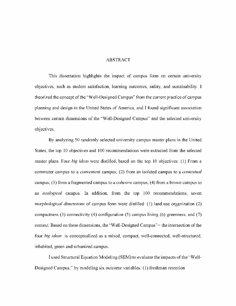
ABSTRACT
This dissertation highlights the impact of campus form on certain university
objectives, such as student satisfaction, learning outcomes, safety, and sustainability. I
theorized the concept of the “Well-Designed Campus” from the current practice of campus
planning and design in the United States of America, and I found significant association
between certain dimensions of the “Well-Designed Campus” and the selected university
objectives.
By analyzing 50 randomly selected university campus master plans in the United
States, the top 10 objectives and 100 recommendations were extracted from the selected
master plans. Four big ideas were distilled, based on the top 10 objectives: (1) From a
commuter campus to a convenient campus; (2) from an isolated campus to a contextual
campus; (3) from a fragmented campus to a cohesive campus; (4) from a brown campus to
an ecological campus. In addition, from the top 100 recommendations, seven
morphological dimensions of campus form were distilled: (1) land use organization (2)
compactness (3) connectivity (4) configuration (5) campus living (6) greenness, and (7)
context. Based on these dimensions, the “Well-Designed Campus”- the intersection of the
four big ideas-is conceptualized as a mixed, compact, well-connected, well-structured,
inhabited, green and urbanized campus.
I used Structural Equation Modeling (SEM) to evaluate the impacts of the “Well-
Designed Campus,” by modeling six outcome variables: (1) freshman retention

rate as a proxy for overall satisfaction with college life, (2) 6-year graduation rate as a
proxy for learning outcome, (3) crime rate as a proxy for safety, (4) STARS as a proxy
for sustainability, (5) students’ commuting behavior, and (6) employees’ commuting
behavior. The statistical population was universities with high research activities in the
United States of America. The hypothesized structural equation models displayed
significant association between three campus form dimensions of urbanism (a composite
variable from the three morphological dimensions of compactness, connectivity, and
context), greenness and campus living with most of the outcome variables considering
control variables. Moreover, the “Well-Designed Campus” can provide a theoretical
framework for future empirical research on either accepting or rejecting common actions
and policies related to campus design.
iv

To my parents and my wife Mahsa

ABSTRACT............................................................................................................................ iii
LIST OF TABLES............................................................................................................... viii
LIST OF FIGURES................................................................................................................ x
ACKNOWLEDGMENTS...................................................................................................xiv
Chapters
1 INTRODUCTION............................................................................................................... 1
1.1 Purpose.....................................................................................................................41.2 Research Questions.................................................................................................51.3 Literature Review....................................................................................................5
1.3.1 Campus Planning and Design in the United States......................................51.3.2 Educating by Design....................................................................................... 71.3.3 Measuring University Quality....................................................................... 9
2 HYPOTHESIS-GENERATING....................................................................................... 16
2.1 The Content Analysis of Campus Master Plans................................................. 162.2 Four “Big Ideas” in Campus Design................................................................... 20
2.2.1 From Commuter Campus to Convenient Campus......................................202.2.2 From Isolated Campus to Contextual Campus...........................................212.2.3 From Fragmented Campus to Cohesive Campus.......................................222.2.4 From Brown Campus to Ecological Campus............................................. 23
2.3 Well-Designed Campus........................................................................................ 24
3 HYPOTHESIS-TESTING.................................................................................................44
3.1 Methodology......................................................................................................... 443.1.1 Sample........................................................................................................... 443.1.2 Data and Measures....................................................................................... 453.1.3 Research Steps and Analytical Methods.................................................... 47
3.2 Results....................................................................................................................503.2.1 Morphological Measures..............................................................................503.2.2 Modeling Campus Form...............................................................................54
TABLE OF CONTENTS

3.2.3 Students’ Satisfaction, Learning Outcome, and Campus Form ................563.2.4 Campus Score................................................................................................593.2.5 Campus Safety and Campus Form ..............................................................623.2.6 Campus Sustainability and Campus Form ................................................. 643.2.7 Students’ Commuting Behavior and Campus Form...................................663.2.8 Employees’ Commuting Behavior and Campus Form.............................. 68
4 SUMMARY AND PERSPECTIVES.............................................................................110
4.1 The Main Findings of the Hypothesis-Generating Phase................................ 1114.2 The Main Findings of the Hypothesis-Testing Phase......................................1124.3 Limitations of Study........................................................................................... 1194.4 Future Research...................................................................................................120
Appendices
A: THE TOP 100 CAMPUS MASTER PLAN RECOMMENDATIONS....................122
B: ANALYTICAL MAPS FOR SELECTED CAMPUSES...........................................130
SELECTED BIBLIOGRAPHY......................................................................................... 191
vii
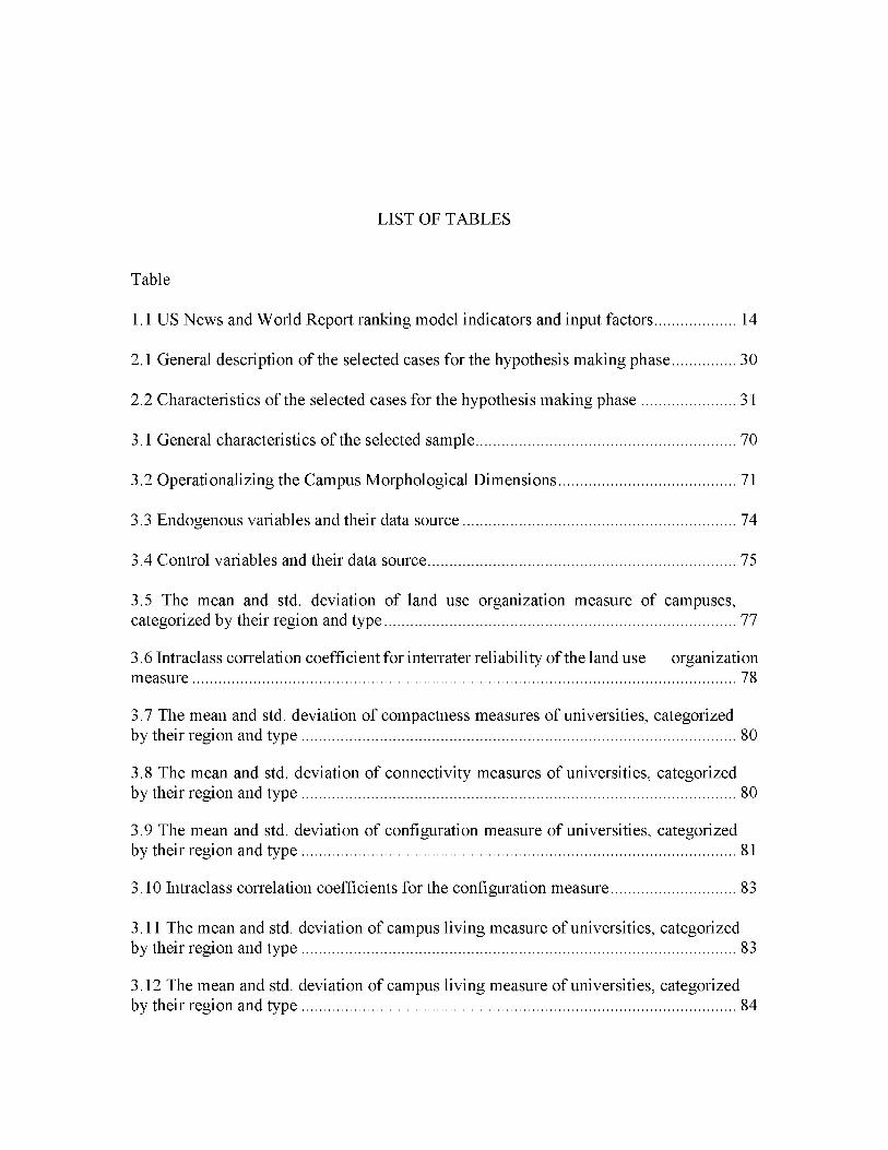
LIST OF TABLES
Table
1.1 US News and World Report ranking model indicators and input factors...................14
2.1 General description of the selected cases for the hypothesis making phase...............30
2.2 Characteristics of the selected cases for the hypothesis making phase......................31
3.1 General characteristics of the selected sample..............................................................70
3.2 Operationalizing the Campus Morphological Dimensions..........................................71
3.3 Endogenous variables and their data source................................................................. 74
3.4 Control variables and their data source..........................................................................75
3.5 The mean and std. deviation of land use organization measure of campuses, categorized by their region and type.................................................................................... 77
3.6 Intraclass correlation coefficient for interrater reliability of the land use organization measure.................................................................................................................................. 78
3.7 The mean and std. deviation of compactness measures of universities, categorized by their region and type........................................................................................................80
3.8 The mean and std. deviation of connectivity measures of universities, categorized by their region and type........................................................................................................80
3.9 The mean and std. deviation of configuration measure of universities, categorized by their region and type........................................................................................................81
3.10 Intraclass correlation coefficients for the configuration measure............................. 83
3.11 The mean and std. deviation of campus living measure of universities, categorized by their region and type........................................................................................................ 83
3.12 The mean and std. deviation of campus living measure of universities, categorized by their region and type........................................................................................................ 84

3.13 The mean and std. deviation of campus living measure of universities, categorize by their region and type........................................................................................................ 85
3.14 The regression weights (ML and Bayesian) in modeling campus form ...................86
3.15 The regression weights (ML and Bayesian) in modeling students’ satisfaction and learning outcome....................................................................................................................87
3.16 The total effects of exogenous variables on 6-year graduation rate..........................88
3.17 Ranking universities based on their campus score.................................................... 91
3.18 The regression weights (ML and Bayesian) in modeling campus crime..................94
3.19 The regression weights (ML and Bayesian) in modeling students’ commuting behavior.................................................................................................................................. 95
3.20 The regression weights (ML and Bayesian) in modeling employees’ commuting behavior.................................................................................................................................. 96
ix

LIST OF FIGURES
Figure
1.1 Research flowchart.......................................................................................................... 13
2.1 The top challenges in front of university campuses..................................................... 32
2.2 Ten most common objectives in the reviewed campus plans......................................33
2.3 The share of each objective from the top recommendations.......................................34
2.4 Design concept of convenient campus...........................................................................35
2.5 University of Michigan, Ann Arbor...............................................................................36
2.6 Concept diagram of contextual campus........................................................................ 37
2.7 Campus map. Left: Yale University; Right: New Mexico State University...............38
2.8 Concept diagram of cohesive campus............................................................................39
2.9 Campus map. Left: University of Washington; Right: University of Utah................40
2.10 Concept diagram of ecological campus...................................................................... 41
2.11 Princeton University.....................................................................................................42
2.12 Morphological dimensions of university campus.......................................................43
3.1 Connectivity map.............................................................................................................97
3.2 Configuration map. The spatial configuration of Yale University............................. 98
3.3 Modeling Campus Form................................................................................................. 99
3.4 Scatter plot. X: Green Score, Y: Living Score............................................................100
3.5 Scatter plot. X: Green Score, Y: Urban Score.............................................................101
3.6 Scatter plot. X: Living Score, Y: Urban Score............................................................102
3.7 Modeling students’ satisfaction and learning outcome.............................................. 103
3.8 Means of Campus Score for each census region and university type....................... 104
3.9 Scatter plot. X: Campus Score, Y: Freshman Retention Rate. R2=0.530 ................ 105
3.10 Scatter plot. X: Campus Score, Y: 6-Year Graduation Rate. R2=0.663................. 106
3.11 Modeling campus crime rate...................................................................................... 107
3.12 Modeling students’ commuting behavior.................................................................. 107
3.13 Modeling employees’ commuting behavior..............................................................109
B.1 Figure ground map, Oklahoma State University........................................................131
B.2 Pervious open space, Oklahoma State University..................................................... 132
B.3 The intensity of tree canopy, Oklahoma State University........................................136
B.4 Figure ground map, University of Alabama............................................................... 134
B.5 Pervious open space, University of Alabama.............................................................135
B.6 The intensity of tree canopy, University of Alabama............................................... 136
B.7 Figure ground map, University of Albany, SUNY................................................... 137
B.8 Pervious open space, University of Albany, SUNY................................................. 138
B.9 The intensity of tree canopy, University of Albany, SUNY.....................................139
B.10 Figure ground map, University of Massachusetts Amherst....................................140
B.11 Pervious open space, University of Massachusetts Amherst..................................141
B.12 The intensity of tree canopy, University of Massachusetts Amherst.....................142
B.13 Figure ground map, Arizona State University, Tempe...........................................143
B.14 Pervious open space, Arizona State University, Tempe.........................................144
B.15 The intensity of tree canopy, Arizona State University, Tempe............................ 145
xi
B.16 Figure ground map, University of Texas at Arlington............................................ 146
B.17 Pervious open, University of Texas at Arlington.................................................... 147
B.18 The intensity of tree canopy, University of Texas at Arlington............................. 148
B.19 Figure ground map of Auburn University................................................................ 149
B.20 Pervious open space, Auburn University................................................................. 150
B.21 The intensity of tree canopy, Auburn University.................................................... 151
B.22 Figure ground map, University of Colorado, Boulder............................................ 152
B.23 Pervious open space, University of Colorado, Boulder..........................................153
B.24 The intensity of tree canopy, University of Colorado, Boulder............................. 154
B.25 Figure ground map, Binghamton University............................................................155
B.26 Pervious open space, Binghamton University..........................................................156
B.27 The intensity of tree canopy, Binghamton University............................................ 157
B.28 Figure ground map, Carnegie Melon University.................................................... 158
B.29 Pervious open space, Carnegie Melon University.................................................. 159
B.30 The intensity of tree canopy, Carnegie Melon University......................................160
B.31 Figure ground map, Case Western Reserve University..........................................161
B.32 Pervious open space, Case Western Reserve University........................................162
B.33 The intensity of tree canopy, Case Western Reserve University........................... 163
B.34 Figure ground map, University of Colorado Denver.............................................. 164
B.35 Pervious open space, University of Colorado Denver............................................ 165
B.36 The intensity of tree canopy, University of Colorado Denver............................... 166
B.37 Figure ground map, Colorado State University.......................................................167
B.38 Pervious open space, Colorado State University.................................................... 168
xii

B.39 The intensity of tree canopy, Colorado State University........................................169
B.40 Figure ground map, University of Connecticut........................................................170
B.41 Pervious open space, University of Connecticut..................................................... 171
B.42 The intensity of tree canopy, University of Connecticut........................................172
B.43 Figure ground map, Cornell University................................................................... 173
B.44 Pervious open space, Cornell University................................................................. 174
B.45 The intensity of tree, Cornell University.................................................................. 175
B.46 Figure ground map, Duke University....................................................................... 175
B.47 Pervious open space, Duke University..................................................................... 177
B.48 The intensity of tree canopy, Duke University........................................................178
B.49 Figure ground map, University of Louisville...........................................................179
B.50 Pervious open space, University of Louisville.........................................................180
B.51 The intensity of tree canopy, University of Louisville............................................ 181
B.52 Figure ground map, University of Nevada............................................................... 182
B.53 Pervious open space, University of Nevada.............................................................183
B.54 The intensity of tree canopy, University of Nevada................................................ 184
B.55 Figure ground map, Oregon State University..........................................................185
B.56 Pervious open space, Oregon State University........................................................186
B.57 The intensity of tree canopy, Oregon State University...........................................187
B.58 Figure ground map, University of Tennessee..........................................................188
B.59 Pervious open space, University of Tennessee........................................................189
B.60 The intensity of tree canopy, University of Tennessee...........................................190
xiii

ACKNOWLEDGMENTS
I would like to give a heartfelt thanks to Dr. Reid Ewing. He was not only my co
chair, but has become my mentor and father figure. His patience, flexibility, genuine caring
and concern, and faith in me during the dissertation process enabled me to complete this
dissertation. I am forever grateful.
I would also like to give special thanks to Dr. Nan Ellin who was also my co-chair
and helped me throughout my dissertation. She has been motivating, encouraging, and
enlightening. I am always touched by her kind and insightful words.
Thirdly, I am very grateful to the other members o f my dissertation committee, Dr.
Arthur C. Nelson, Dr. Jonathan Butner, and Dr. Sarah Hinners. Their academic support and
input greatly appreciated.
In addition, I would like to thank my colleagues and friends, Allison Spain, David
Profit, Shima Hamidi, Andrea Garfinkel Castro, Philip Stoker, Katherine Kittrell, Matt
Miller, Keuntae Kim and the other doctoral students for their support, and for the many
precious memories along the way.
Last, but not least, the successful completion of this dissertation research would
have not been possible without the support o f my family and my wife, Mahsa. I would like
to express my deep love and appreciation to them.
CHAPTER 1
INTRODUCTION
My dissertation research began from a curiosity, an interest, and a demand. Four
university campuses, two in Iran and two in the United States, have been my home and
sanctuary for the last 14 years. Looking back, I can clearly see how each university has
enriched my life not just through academic education, but mainly through nonacademic
experiences and background activities associated with college life. I have established
friendships, developed social skills, and made numerous lasting memories. Of course, each
university was unique. At Shahid Beheshti University, I found my lifetime friends sitting
on campus grass. At the University of Tehran, I rediscovered my hometown finding all the
“cool” places around the campus. In Ann Arbor, Michigan I felt what it means to be part
of an academic community/village for the first time. And I will leave the University of
Utah with the memory of its astonishing mountain views. Overall, I appreciate how each
campus reinforces the unique quality of its institution, and I regret the presence of
unfulfilled potentials. As an urban designer and planner, I’m curious to know more about
the potential contributions of campuses to universities’ eminence.
Evaluating urban design concepts with various analytical methods is my primary
research interest. The application of spatial and GIS analysis techniques, typo-
morphological approaches and statistical modeling tools for the creation and assessment of
urban design conceptual frameworks is intriguing to me. This dissertation is an opportunity

for me to perform an in-depth study of the interactions between analytical techniques and
macroscale design concepts.
Campus design can be applied to both microscale (specific college and university
projects) and macroscale designs (organizing the campus, or campus sector, as a functional
and visual unit). Campus designers used to follow a few macroscale ideas or formal
typologies before World War II, such as the quadrangle, Beaux-Arts, pastoral/picturesque,
or a hybrid of these types. With the unprecedented expansion of university campuses in the
United States of America in the post-WWII era, the main focus of campus leaders was
towards individual buildings rather than master plans. Today, the result of that practice is
the fuzziness o f the big picture o f contemporary campus design. The lack of a macroscale
design idea and concentration on individual buildings produced drive-through, sprawling,
fragmented, and isolated campuses (Coulson et al., 2010; Turner, 1984). Some may argue
that with the complexity and diversity of modern universities’ challenges, missions, and
policies, it is less relevant to think about a common “big idea” for campus master plans.
To some extent, that may be true. However, for practitioners, the main advantage of
knowing about the common “big ideas” is to be more conscious and cautious about
adopting or rejecting one of these design norms. And for campus scholars, it can provide a
theoretical framework to assess the impacts o f common practice.
Ultimately, the purpose of this research is to propose and evaluate the concept of
the “Well-Designed Campus” as the overlap of various macroscale design concepts for
creating a sustainable and livable learning environment. My dissertation research has two
main stages (see Figure 1.1): (1) hypothesis making - qualitative approach, (2) hypothesis
testing - quantitative approach. In the first stage, I conceptualized a normative theory from
2

3
current campus planning and design practice and introduced the concept of the “Well-
Designed Campus.” In the second stage, I assessed the impact of the proposed macroscale
design concept on the desired outcomes, such as overall student satisfaction, learning
environment, safety and sustainability.
I started this research by visiting various great university campuses in the United
States of America and reviewing relevant literature on the subject, which helped me refine
my research question. The next step was the content analysis of 50 randomly selected
campus master plans in the United States. I extracted the top common objectives and most
frequent recommendations from the selected campus master plans. From the most frequent
recommendations, I conceptualized seven macroscale morphological dimensions for
university campuses: (1) Land use organization: How mixed is the distribution of sport,
research, residence, and different academic facilities? (2) Compactness: the degree of
campus density and relative proximity of buildings; (3) Connectivity: the degree of street
network connectivity within the campus and to the surrounding area; (4) Configuration:
the strength of campus spatial organization; (5) Campus living: the degree of on campus
living; (6) Greenness: the degree of naturalness/greenness; and (7) Context: the degree of
urbanism of the surrounding area.
From a literature review, I confirmed the importance of the seven morphological
dimensions for campus quality. Also, from the literature review I operationalized
morphological dimensions, and selected six outcome variables: (1) freshman retention rate
as a proxy for overall satisfaction with college life,1 (2) graduation rate as a proxy for
1 About one in three 1st-year students won't make it back for sophomore year. The reasons range from personal problems and loneliness to academic struggles and expenses (Roberts, & Styron, 2010).
learning environment, (3) crime rate as a proxy for safety, (4) sustainability rate/STARS
as a proxy for sustainability, (5) students’ commuting behavior, and (6) employees’
commuting behavior.
For the hypothesis testing phase, I measured seven morphological dimensions for
103 university campuses with high research activities in the United States (the total
population is 206, according to the Carnegie classification 2010). I measured five
dimensions quantitatively, but had to rate two dimensions - Land use organization and
Configuration - qualitatively. My hypothesis (based on the current campus design practice)
is that a mixed, compact, well-connected, well-structured, inhabited, green, and urbanized
campus is a “Well-Designed Campus.” Using Structural Equation Models, I modeled the
four outcome variables in terms of the measured morphological dimension and an overall
campus-score while considering control variables.
1.1 Purpose
Designers and planners believe that design matters and plans are helpful. That is
why campus master plans, generally, recommend a set of design and planning actions to
fulfill university goals and objectives as higher education institutions. The review of
different campus master plans demonstrates undeniable similarities among their
recommendations. However, the validity of the proposed recommendations has not been
tested. Most publications about campus planning/design are by practitioners (Chapman,
2006; Coulson, Roberts & Taylor, 2010; Dober, 1996; Kenney, Dumont, & Kenney, 2005;
Toor, & Havlick; 2004) and few academic studies verify the default assumptions of campus
planning practice. As Dober (1996) observed, “Lacking an organized body of research or
theory, campus planning is likely to be continued on a pragmatic basis” (p. 12). This
4

research is an attempt to provide a theoretical framework for evaluating common “big
ideas” in contemporary campus planning and design practice.
1.2 Research Questions
Main question:
• What are the principal features of contemporary university campus planning
and design, and when implemented, are they correlated with university
objectives such as student success and satisfaction, and campus safety and
sustainability?
Other questions:
• What are the most common challenges, obj ectives, and recommendations in the
campus master plans of the U.S.?
• How can the physical form of university campuses best be analyzed?
• How can the research universities be rated and ranked based on their campus
quality?
1.3 Literature Review
1.3.1 Campus Planning and Design in the United States
The roots of campus planning and design go back to medieval Europe (see Coulson
et al., 2010; Dober, 1996; Turner, 1984), but it was mainly in America where modern
university campuses evolved. One of the significant periods in the evolution of campus
form was when Thomas Jefferson, the third president of the United States and founder of
the University of Virginia, embraced ideals of the Enlightenment and wanted to express
these same sentiments of freedom and openness of mind through the built form of a
5

university campus. The traditional quadrangles and built form of the universities found in
the United Kingdom and Europe were reformed by architects and planners in the United
States (Turner, 1984). American architects and planners adopted certain architectural styles
and features from European and Oxbridge models; however the visual presence of the
buildings - their connection with the landscape, a university’s mission, and its connection
with the broader community - were designed so as to communicate a symbolic departure
from English aristocratic and medieval ways of thought (Steinmetz, 2009).
The evolution of campus form is a continuous process, and in each era it faces its
unique challenges. Today, throughout North America, college and university campuses
have experienced growth in numbers of students, staff, and faculty over the last 40 years.
Per capita automobile use and ownership have increased significantly to the point where
almost every urban campus faces serious impacts from car traffic and parking shortages.
Discrete boundaries between the university and the neighborhood can create an isolated
campus. Unaffordable housing can make students commute long distances. A low density
campus, low quality of housing, inappropriate zoning, hostile town and gown relationships,
reputation as a “party school,” social injustice, the shifts in learning practices and in the
global education market are also potential threats to university campuses (Chapman, 2006;
Coulson, Roberts, & Taylor, 2010; Coulson, Roberts, & Taylor, 2014; Dober, 1996;
Kenney et al., 2005; Mitchell & Vest, 2007; Strange & Banning, 2001; Turner, 1984).
Campus projects can address this wide range of problems and concerns in different
ways. Coulson, Roberts, and Taylor (2014) discuss “trends” in contemporary campus
design. These trends are adaptive reuse of buildings and facilities, starchitecture, hub
buildings, interdisciplinary science research buildings, commercial urban development,
6

7
large-scale campus expansions, and revitalizing master plans. This research will be focused
on the last o f these. Master plans express the idea or vision of institution, guide growth and
change, and reinforce the strategic plan (Dober, 1996). Therefore, the scope of campus
plans can be vast and diverse. But according to Kenney, Dumont, and Kenney (2005) a
comprehensive campus plan should follow these nine principles:
• Giving precedence to the overall plan over individual buildings and spaces
• Using compactness (density) and mixing campus uses to create vitality and
interaction
• Creating a language of landscape elements that expresses the campus’s
individuality and relationship to its regional context
• Embracing environmental considerations
• Taming the automobile
• Utilizing campus architecture to further placemaking
• Integrating technology
• Creating a beneficial physical relationship with the neighborhood
• Bringing meaning and beauty to the special places on campus
In the next chapter, the hypothesis making phase, I will show which of these
principles are more commonly used in master plans and how practitioners address them.
1.3.2 Educating by Design
Can the physical form of universities help universities achieve their missions and
objectives? The influence of physical environment on academic and nonacademic
objectives o f universities is an established research topic among higher education and
environmental psychology scholars (Boyer, 1987; Cox & Orehovec, 2007; Griffith, 1994;

8
Jessup-Anger, 2012; Long, 2014; Pope et al., 2014; Schuetz, 2005; Strange & Banning,
2001; Temple, 2008; Thelin & Yankovich, 1987). The physical form of campuses is often
among the most important factors in creating a positive first impression of an institution
among prospective students (Boyer, 1987; Griffith, 1994; Stuner, 1973; Thelin &
Yankovixh, 1987). The basic layout of the campus, the quality of open spaces, the
accessibility of parking lots, and the design of buildings, such as residence halls, libraries,
or student unions, can shape initial attitudes in subtle ways.
The impact of physical environment on behavior can be conceptualized as
possibilism or probabilism (Lang, 2005). The physical environment can be the source of
opportunities or can impact the probability of certain behaviors. For example, the presence
of a convenient and attractive gathering space within the core of campus enhances the
opportunity for students to socialize on campus; or having sport facilities far from campus
can decrease the probability of the facilities being used. Strange and Banning (2001) argue
that “although features of the (campus) physical environment lend themselves theoretically
to all possibilities, the layout, location, and arrangement of space and facilities render some
behaviors much more likely, and thus more probable, than others” (p. 56).
The impact of university campus design can be understood by examining the
campus from the view point of a pedestrian (Banning, 1993). A good campus not only
provides a safe, convenient, and pleasurable walk for pedestrians, but also adds “sense of
inclusion,” “sense of place,” and “learning” to the walking experience (Strange & Banning,
2001). For example, crossing an active quadrangle, or a plaza can create an opportunity for
students to socialize and feel the sense of belonging and inclusion (Banning & Bartels,
1993). Harmony in the architectural design of buildings and the landscaping of campus can
enhance the “sense of place.” In addition, a legible campus spatial structure can increase
the probability of students becoming engaged in various intellectual activities across the
campus. Perhaps locating the main library on the main pedestrian pathway with a
welcoming entrance can encourage students to enter the library and use its resources.
However, among the many methods employed to foster learning, the use of physical
environment is perhaps the most neglected aspect.
1.3.3 Measuring University Quality
To identify common measures of universities’ quality, I conducted a literature
review. This literature review helped me select measurable and valid outcomes and control
variables for the hypothesis testing phase. Brooks (2005) classified the assessment of
university quality in three research areas: reputation, faculty research, and student
experience. The most widely cited and the first reputational study was in 1925 by the
president of Miami University of Ohio, which was the ranking of the 38 top Ph.D.-granting
institutions out of the 65 institutions at that time (Hughes, 1925).
Many contemporary reputational assessments are in the form of rankings and
ratings designed by commercial media, driven by profit motives. U.S. News and World
Report is one of the private institutions that produces college rankings every year. Their
ranking is mainly based on the survey data coming from the colleges and universities
themselves. Their other sources of data include (1) the American Association of University
Professors (faculty salaries), (2) the National Collegiate Athletic Association (graduation
rates), (3) the Council for Aid to Education (alumni giving rates) and (4) the U.S.
Department of Education's National Center for Education Statistics (information on
financial resources, faculty, SAT and ACT admissions test scores, acceptance rates and
9
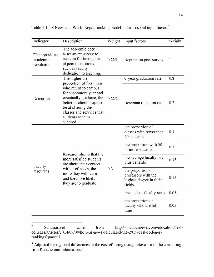
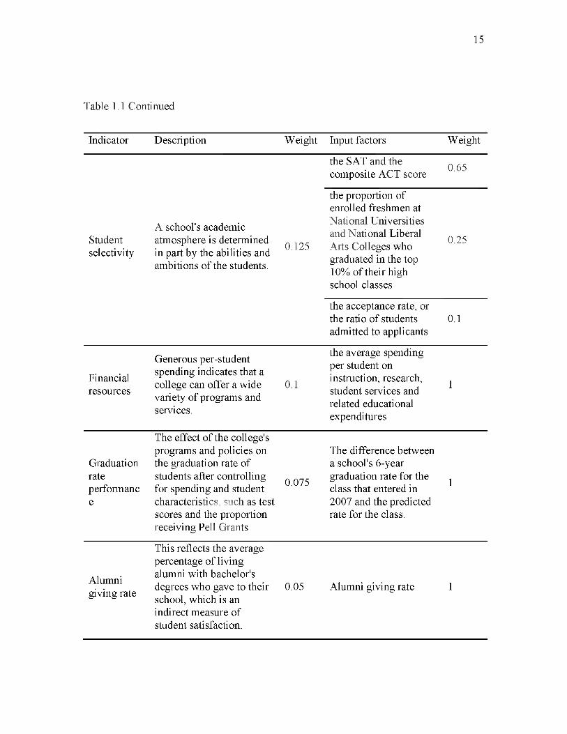
graduation and retention rates). Table 1.1 shows their ranking model indicators, their
weights and input factors. Other commercial rating systems, such as College Factual, use
very similar variables in their ratings.
Brooks (2005) classified all student experience measures into four main categories:
program characteristics, program effectiveness, student outcomes, and student satisfaction.
The last category can be better linked with students’ campus life experiences. One of the
most comprehensive research studies in this field has been conducted by the Indiana
University Center for Postsecondary Research. Partnering with the Carnegie Foundation
for the Advancement o f Teaching and the Association of American Colleges and
Universities, they annually conduct the National Survey of Student Engagement (NSSE).
NSSE measures the extent of student engagement with faculty, with each other, and with
their studies in educationally effective activities. Unfortunately, it is not possible to use this
dataset in this research because, under the terms of their institutional participation
agreement, institutionally identified data cannot be provided to other researchers.
Pike (2004) has found that NSSE data do not have a strong relationship to U.S.
News rankings, indicating that student impressions of their educational experiences vary
irrespective of institutional characteristics. That can also suggest that cross-institutional
comparisons of survey data, such as NSSE, must be made with caution, since students may
have different expectations o f different institutions.
University quality is a growing topic in the economics literature. Existing studies
o f the effects o f university quality on wages typically rely on few proxy variables for
university quality (Bacolod et al., 2009; Belfield et al., 2011; Black et al., 2005; Black &
Smith 2004; Black & Smith, 2006; Daniel et al. 1997; Fitzgerald & Burns, 2000; Long,
10

2008; Monks, 2000; Zhang, 2005). In this field of research, university quality measurement
typically includes three aspects of quality: student selectivity, faculty resources, and
students’ satisfaction. The most common variables to estimate these aspects (factors) are
faculty-student ratio, rejection rate, freshman retention rate, mean SAT score, and mean
faculty salaries (Bacolod et al., 2009; Belfield et al., 2011; Black & Smith 2004; Black et
al., 2005; Black & Smith, 2006; Daniel et al. 1997; Fitzgerald & Burns, 2000; Monks,
2000; Long, 2008; Zhang, 2005).
The only available data on campus sustainability are from the Sustainability
Tracking and Assessment Rating System (STARS). STARS is “a transparent, self
reporting framework for colleges and universities to measure their sustainability
performance” (STARS website, stars.aashe.org). STARS was developed by the
Association for the Advancement of Sustainability in Higher Education (AASHE). STARS
participants pursue credits and may earn points in order to achieve a STARS Bronze,
Silver, Gold or Platinum rating. The rating criteria are organized into four categories:
Academics, Engagement, Operations, and Planning and Administration. Since STARS
launched in 2010, 406 institutions have submitted STARS reports. About 40% of them are
doctoral institutions in the United States of America. From the total participants, 8% of
institutions choose not to participate in the rating; 22% earned Bronze, 49% Silver, and
21% Gold ratings.
Measuring university qualities is not an easy task, but as described, different proxy
variables have been used for this purpose. However, quantifying physical campus qualities
has no precedent in the literature. In the next chapter, through the content analysis of 50
campus master plans, I theorized seven morphological dimensions of campus form that can
11
12
contribute to a “Well-Designed Campus.” This would be an essential step for measuring
campus qualities.

13
F indings and discussions
an in terest, a curiosity , and a question
Figure 1.1 Research flowchart
14
Table 1.1 US News and World Report ranking model indicators and input factors2
Indicator Description Weight Input factors Weight
Undergraduateacademicreputation
The academic peer assessment survey to account for intangibles at peer institutions, such as faculty dedication to teaching.
0.225 Reputation peer survey 1
The higher the proportion of freshmen who return to campus for sophomore year and eventually graduate, the better a school is apt to be at offering the classes and services that students need to succeed.
6-year graduation rate 0.8
Retention 0.225freshman retention rate 0.2
the proportion of classes with fewer than 20 students
0.3
Research shows that the more satisfied students are about their contact
the proportion with 50 or more students 0.1
Facultyresources 0.2
the average faculty pay, plus benefits3 0.35
with professors, the more they will learn and the more likely they are to graduate.
the proportion of professors with the highest degree in their fields
0.15
the student-faculty ratio 0.05
the proportion of faculty who are full time
0.05
2 Summarized table from http://www.usnews.com/education/best- colleges/articles/2014/09/08/how-us-news-calculated-the-2015-best-colleges- rankings?page=1
3 Adjusted for regional differences in the cost of living using indexes from the consulting firm Runzheimer International
15
Table 1.1 Continued
Indicator Description Weight Input factors Weight
the SAT and the composite ACT score 0.65
Studentselectivity
A school's academic atmosphere is determined in part by the abilities and ambitions of the students.
0.125
the proportion of enrolled freshmen at National Universities and National Liberal Arts Colleges who graduated in the top 10% of their high school classes
0.25
the acceptance rate, or the ratio of students admitted to applicants
0.1
Financialresources
Generous per-student spending indicates that a college can offer a wide variety of programs and services.
0.1
the average spending per student on instruction, research, student services and related educational expenditures
1
Graduationrateperformance
The effect of the college's programs and policies on the graduation rate of students after controlling for spending and student characteristics, such as test scores and the proportion receiving Pell Grants
0.075
The difference between a school's 6-year graduation rate for the class that entered in 2007 and the predicted rate for the class.
1
Alumni giving rate
This reflects the average percentage of living alumni with bachelor's degrees who gave to their school, which is an indirect measure of student satisfaction.
0.05 Alumni giving rate 1

CHAPTER 2
HYPOTHESIS-GENERATING
2.1 The Content Analysis o f Campus Master Plans
“No two campuses are alike, nor would we want them to be. The genius loci o f the U.S. campus is embodied in the enormous variety o f geographic, cultural, and climatic circumstances in which campuses have evolved.” (Chapman, 2006, p. 30)
If each campus is unique, should we expect unique recommendations on their
campus plans as well? Or should we expect some level of similarity between the
challenges, objectives and recommendations? To answer this question, I reviewed 50
university campus master plans. They have been selected randomly through a web search
for the keywords of “university campus master plan.”4 I had two criteria for selecting my
case:
4 Selected universities are Auburn University, Boise State University, Brown University, Bucknell University, Carnegie Mellon University, Clemson University, Coastal Carolina University, Cornell University, Drexel University, Duke University, Indiana University, Kansas State University, Lehigh University, Longwood University, Princeton University, Purdue University at Calumet, Purdue University at West Lafayette, Radford University, South Dakota State University, Southern Oregon University, Stanford University, University o f Alaska at Anchorage, University o f California at Berkeley, University of Colorado at Boulder, University o f Delaware, University o f Illinois at Chicago, University o f Iowa, University o f Maine, University o f Massachusetts at Amherst, University of Memphis, University o f Michigan, University o f New Hampshire, University o f North Carolina at Charlotte, University o f North Florida, University o f Richmond, University o f South Alabama, University of South Carolina, University of Tennessee, University of Texas at Arlington, University o f Texas at Austin, University o f Utah, University of Vermont, University of Washington at Seattle, University of Wisconsin at La Crosse, University of Wisconsin at Milwaukee, Valparaiso University, Villanova University, Wake Forest University, Western Illinois University, and Yale.

(1) The master plan should be produced in 2000 or later, and (2) the challenges,
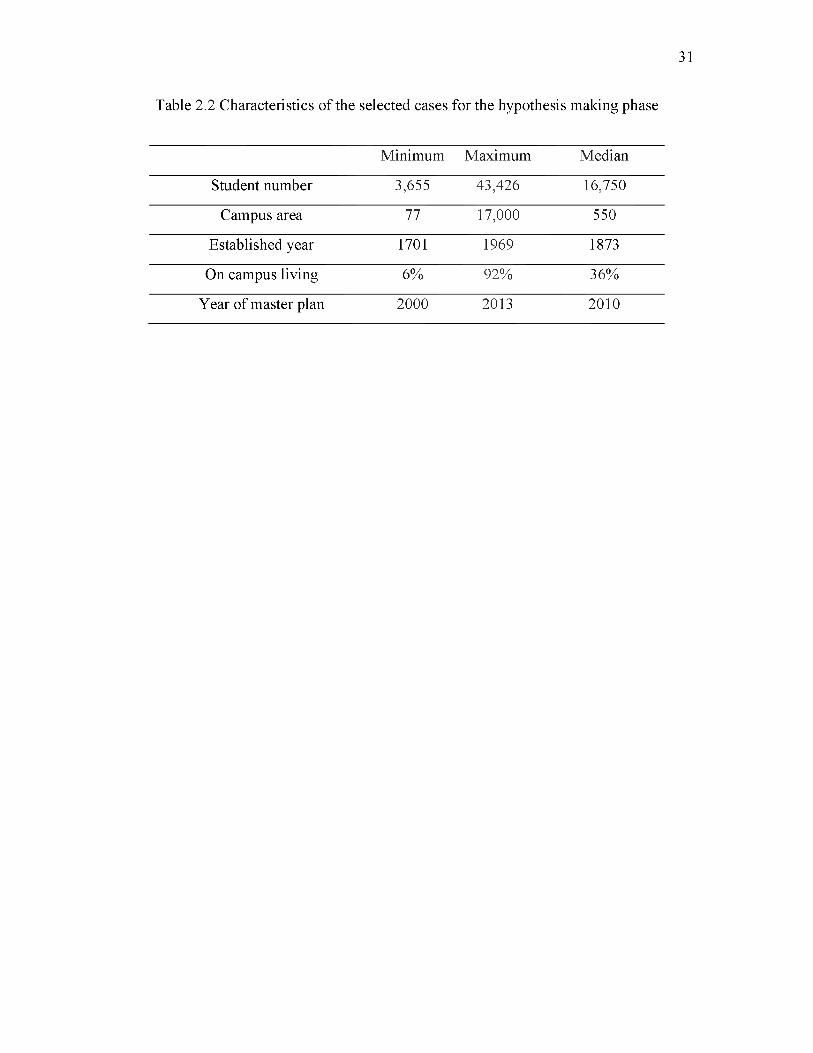
objectives and recommendations should be clearly stated. Table 2.1 and 2.2 show some
characteristics of the selected universities. Of the selected universities, 72% are public;
28% are land-grant universities; 72% are located in an urban setting. The campuses range
in size from 77 to 17,000 acres, with a median size of 550 acres. The master plans for these
universities were last updated and adopted in 2010, on average.
The survey shows that there are significant similarities between universities in
terms of challenges, objectives, and recommendations. This doesn’t mean that generic
recommendations are acceptable; it just indicates that despite all the differences,
universities share related challenges and objectives. This review shows that the top
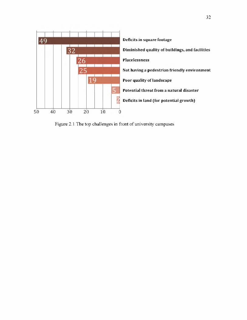
challenges for university campuses are:
1. Deficits in square footage.
2. Diminished quality of buildings and educational facilities, and infrastructure.
3. Disconnected campus from its context and students’ life (Placelessness).
4. Drive-through campus (uninterrupted parking areas and pedestrian unfriendly
environment).
5. Poor quality of landscape.
6. Potential threat or recovering from a natural disaster.
7. Deficits in land (for potential growth).
This finding shows that almost all campuses have to solve their “deficits in square
footage,” but only two have “deficits in land” as a main challenge (see Figure 2.1).
Remarkably, although 72% of these campuses are in urban settings, they still have enough
space on campus for additional infill projects. The other finding is that four of these
17

challenges (2 to 5), are about the quality of infrastructure, buildings, landscaping, and
campus open spaces. However, quality is such a broad term and needs to be
operationalized.
Looking at the common objectives of master plans can better define which qualities
are more likely to be at the center of campus planners/designers’ interest. The most
common objectives in the reviewed campus plans are:
1. Walkability: Redefining the movement systems throughout the campus to be
functional, safe, and legible.
2. Sense of community: Reinforcing a sense of community within campus by
encouraging student engagement in campus activities and inspiring learning
and collaboration outside the classroom.
3. Livability and safety: Expanding student housing and providing quality
physical facilities and a healthy and secure environment.
4. Environmental sustainability: Planning and building in an environmentally
sustainable manner.
5. Landscaping: Preserving and strengthening the identity of the campus with its
natural features and maintaining a high quality memorable landscape.
6. Town-gown relationship: Integrating the campus with the surrounding
neighborhoods.
7. Identity: Strengthening the identity of the campus as a continuously evolving
environment while respecting campus history.
8. Imageability: Creating a memorable and beautiful campus.
18

9. Partnering: Partnering with private developers and communities to support
local and regional prosperity and secure the University’s financial future.
10. Learning environment: Cultivating a learning environment that supports
intellectual curiosity, academic achievement, interdisciplinary research, and
teaching and personal growth.
Figure 2.2 shows the frequency of each objective in the reviewed campus plans. At
first, it is unexpected to see walkability and sense o f community on the top and cultivating
learning environment at the bottom of this list. However, two reasons can be imagined for
this ranking. First, these objectives are not totally independent. For example, to create a
better learning environment, we can promote livability and sense of community on campus.
In other words, some objectives can be nested in the others. Second, there are not many
physical interventions in a campus environment that can directly address learning
outcomes. Therefore, promoting walkability, for example, can be more practical than
improving learning through campus planning.
Appendix A lists the 100 most common recommendations in the reviewed campus
plans. These recommendations are categorized based on the common objectives in campus
plans. Instead of categorizing based on the 10 most common objectives, I used nine
categories. “Learning environment” is not used as a category, because of its overlap with
other objectives. Figure 2.3 shows the share of each objective from the top 100
recommendations, and the total number of recommendations repeated in all 50 master plans
which is 2,508 cases. For example, the number of recommendations addressing
environmental sustainability is only 7 out of 100; however, the frequency of these
recommendations in all cases is much higher. 13% of all recommendations in all 50 master
19
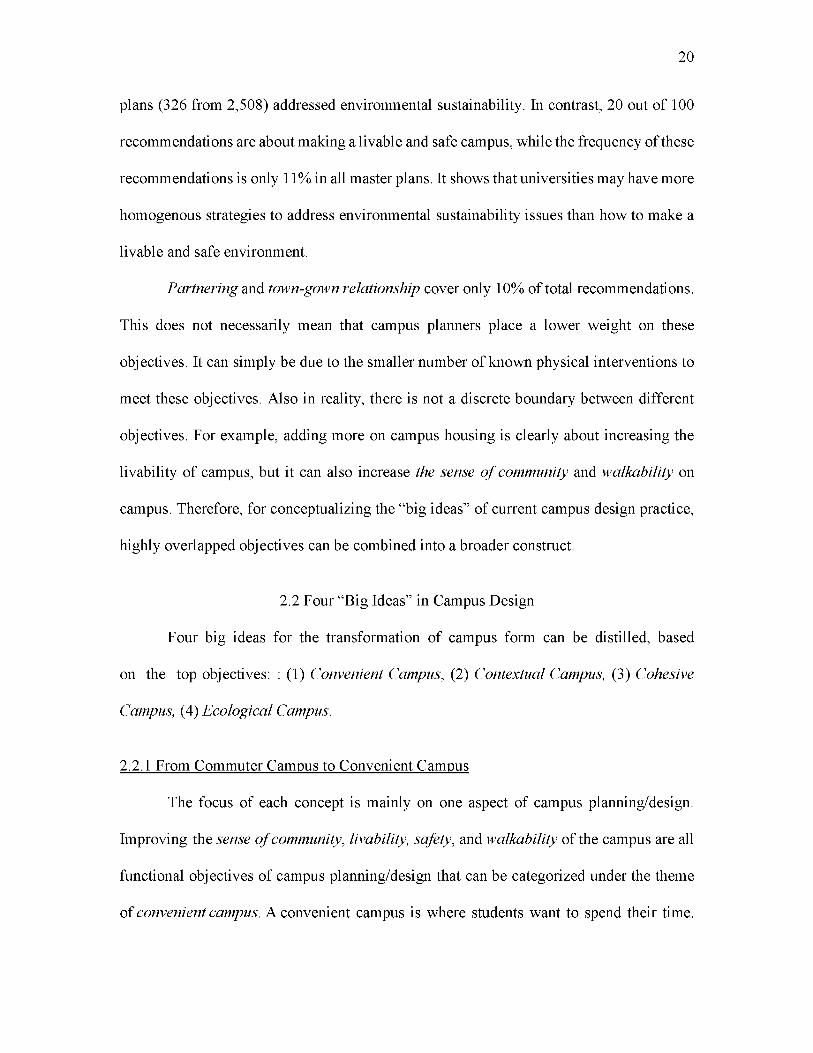
plans (326 from 2,508) addressed environmental sustainability. In contrast, 20 out of 100
recommendations are about making a livable and safe campus, while the frequency of these
recommendations is only 11% in all master plans. It shows that universities may have more
homogenous strategies to address environmental sustainability issues than how to make a
livable and safe environment.
Partnering and town-gown relationship cover only 10% of total recommendations.
This does not necessarily mean that campus planners place a lower weight on these
objectives. It can simply be due to the smaller number of known physical interventions to
meet these objectives. Also in reality, there is not a discrete boundary between different
objectives. For example, adding more on campus housing is clearly about increasing the
livability of campus, but it can also increase the sense o f community and walkability on
campus. Therefore, for conceptualizing the “big ideas” of current campus design practice,
highly overlapped objectives can be combined into a broader construct.
2.2 Four “Big Ideas” in Campus Design
Four big ideas for the transformation of campus form can be distilled, based
on the top objectives: : (1) Convenient Campus, (2) Contextual Campus, (3) Cohesive
Campus, (4) Ecological Campus.
2.2.1 From Commuter Campus to Convenient Campus
The focus of each concept is mainly on one aspect of campus planning/design.
Improving the sense o f community, livability, safety, and walkability of the campus are all
functional objectives of campus planning/design that can be categorized under the theme
of convenient campus. A convenient campus is where students want to spend their time.
20
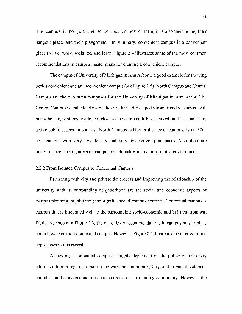
The campus is not just their school, but for most of them, it is also their home, their
hangout place, and their playground. In summary, convenient campus is a convenient
place to live, work, socialize, and learn. Figure 2.4 illustrates some of the most common
recommendations in campus master plans for creating a convenient campus.
The campus of University of Michigan in Ann Arbor is a good example for showing
both a convenient and an inconvenient campus (see Figure 2.5). North Campus and Central
Campus are the two main campuses for the University of Michigan in Ann Arbor. The
Central Campus is embedded inside the city. It is a dense, pedestrian friendly campus, with
many housing options inside and close to the campus. It has a mixed land uses and very
active public spaces. In contrast, North Campus, which is the newer campus, is an 800-
acre campus with very low density and very few active open spaces. Also, there are
many surface parking areas on campus which makes it an auto-oriented environment.
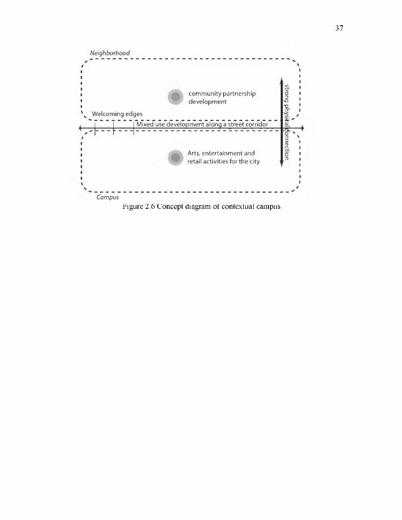
2.2.2 From Isolated Campus to Contextual Campus
Partnering with city and private developers and improving the relationship of the
university with its surrounding neighborhood are the social and economic aspects of
campus planning, highlighting the significance of campus context. Contextual campus is
campus that is integrated well to the surrounding socio-economic and built environment
fabric. As shown in Figure 2.3, there are fewer recommendations in campus master plans
about how to create a contextual campus. However, Figure 2.6 illustrates the most common
approaches in this regard.
Achieving a contextual campus is highly dependent on the policy of university
administration in regards to partnering with the community, City, and private developers,
and also on the socioeconomic characteristics of surrounding community. However, the
21

physical campus can also be planned and designed in such a way that it either promotes or
weakens the potential interactions between campus and its context.
For example, the central campus of Yale University like the central campus of
University of Michigan is embedded inside a small city. The spatial structure of campus is
the natural extension of New Haven’s spatial structure. Its public spaces are highly
accessible for the surrounding community, and also the retail services of neighborhood are
very accessible for campus residents. In contrast, New Mexico State University is
surrounded by highways, and therefore deprived of meaningful interaction with the
“outside world” (see Figure 2.7).
2.2.3 From Fragmented Campus to Cohesive Campus
The physical and more artistic goals of campus planning/design are improving the
legibility, imageability and identity of campus. This set of objectives can create the third
theme of transformation termed cohesive campus. Cohesive campus is similar to what
Chapman (2006) described as “a designed place, deliberately conceived by its builders to
impart a distinct aesthetic effect,” (p. 67) or “the campus as a work of art” (p. 4).
Traditionally a big portion of campus master plans has focused on this aspect by
establishing design guidelines and design codes. Figure 2.8 illustrates the most common
recommendations in this regard.
Because of the rich history of campus design and planning in the U.S., there are
many good examples of cohesive campus all around the country. University of Washington
in Seattle is one of them (see Figure 2.9). The main asset of the campus is its well-designed
spatial structure that has beautifully organized the entire campus. Moreover, the well-
designed sequence of spaces leads to a pleasant walk on campus. The other significant
22
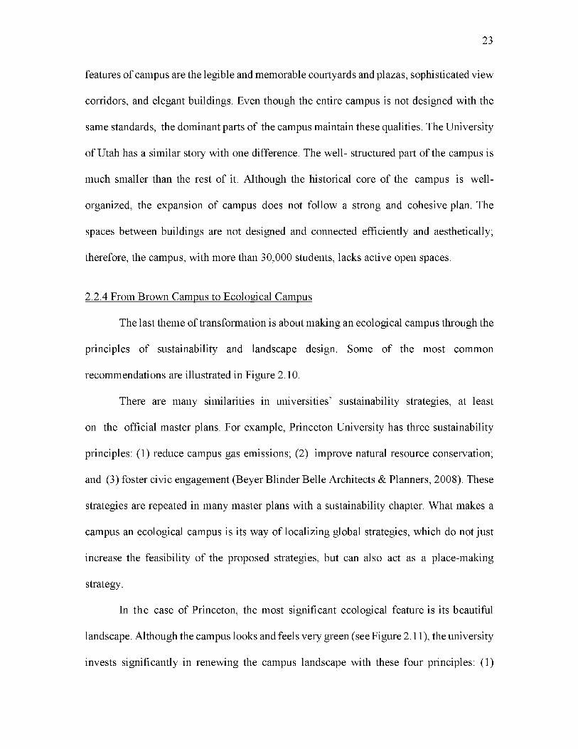
features of campus are the legible and memorable courtyards and plazas, sophisticated view
corridors, and elegant buildings. Even though the entire campus is not designed with the
same standards, the dominant parts of the campus maintain these qualities. The University
of Utah has a similar story with one difference. The well- structured part of the campus is
much smaller than the rest of it. Although the historical core of the campus is well-
organized, the expansion of campus does not follow a strong and cohesive plan. The
spaces between buildings are not designed and connected efficiently and aesthetically;
therefore, the campus, with more than 30,000 students, lacks active open spaces.
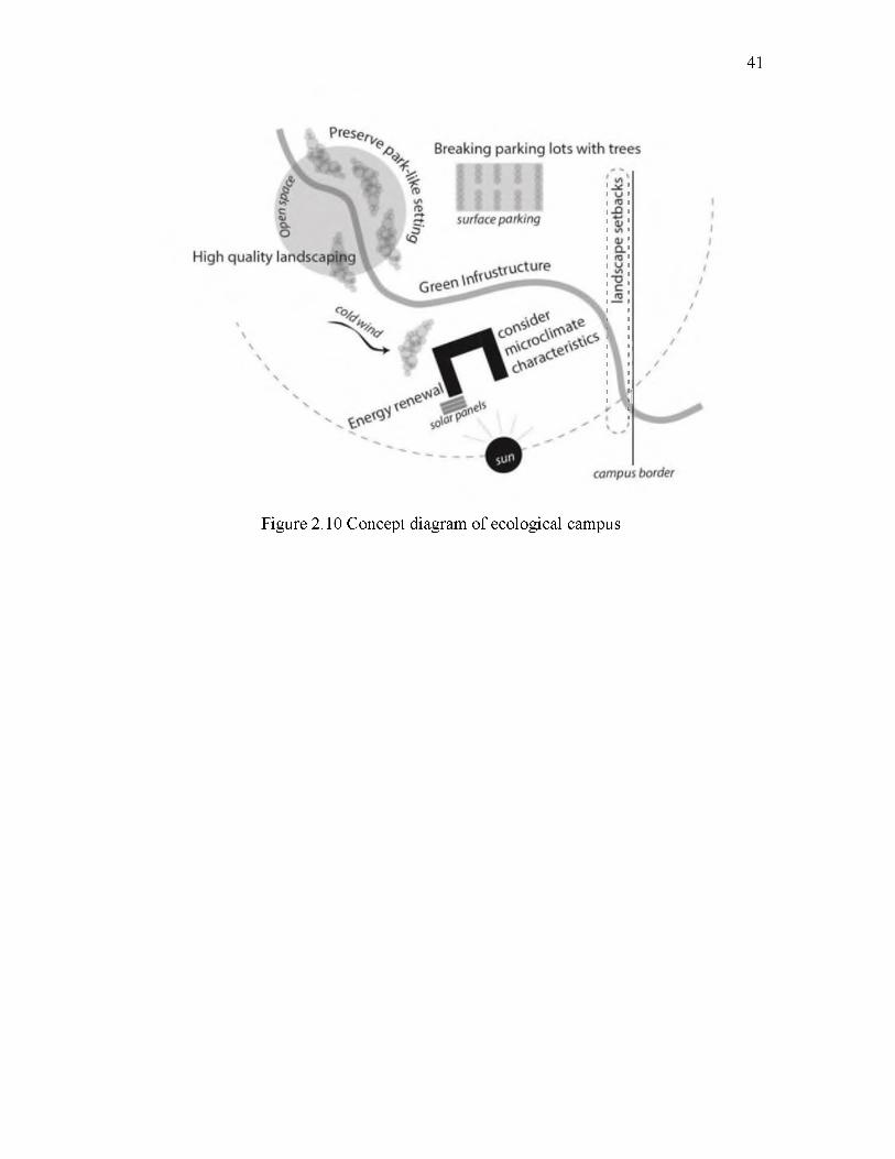
2.2.4 From Brown Campus to Ecological Campus
The last theme of transformation is about making an ecological campus through the
principles of sustainability and landscape design. Some of the most common
recommendations are illustrated in Figure 2.10.
There are many similarities in universities’ sustainability strategies, at least
on the official master plans. For example, Princeton University has three sustainability
principles: (1) reduce campus gas emissions; (2) improve natural resource conservation;
and (3) foster civic engagement (Beyer Blinder Belle Architects & Planners, 2008). These
strategies are repeated in many master plans with a sustainability chapter. What makes a
campus an ecological campus is its way of localizing global strategies, which do not just
increase the feasibility of the proposed strategies, but can also act as a place-making
strategy.
In the case of Princeton, the most significant ecological feature is its beautiful
landscape. Although the campus looks and feels very green (see Figure 2.11), the university
invests significantly in renewing the campus landscape with these four principles: (1)
23
24
invent within the traditional pattern of campus-making; (2) translate the typography into
campus form; (3) reassert the presence of the woodland threshold; (4) anticipate the impact
of increased land management and environmental pressures (Beyer Blinder Belle
Architects & Planners, 2008). With this investment, Princeton not only maintains its unique
asset (the landscape), it can address a range of sustainability objectives such as promoting
walking and biking on campus, improving water quality through green storm water
management systems, creating a student run organic garden, and preserving the
biodiversity of natural and cultivated landscapes.
2.3 Well-Designed Campus
Can we extract a single macroscale design concept from the current practice of
campus planning/design? The first step to hypothesize such a construct, termed a “Well-
Designed Campus,” is identifying the attributes of campus form (morphological
dimensions) that are claimed to have impact on the most common objectives of campus
planning and design.
I conceptualized the morphological dimensions from the most common campus
master plan recommendations. I also confirmed the significance of these concepts by
reference to the campus design literature. These morphological dimensions are:
(1) Land Use Organization: the degree to which sport, research, residence, and
different academic facilities are mixed. Common campus recommendations for
this attribute are:
• Integrating academic and research activities in shared facilities,
• Recognizing distinct communities of disciplines,
• Intensifying the overlap and magnitude of campus workplace, residential,
and activities
• Relocating low-intensity land uses like athletic fields, greenhouses and
barns from the campus core.
According to Kenny et al. (2005), the social, academic, and fiscal benefits of mixing
campus uses include: 1) increased collegiality and community, 2) enhanced learning, 3)
safety, 4) competitive admissions, and 5) flexibility for growth. Kenny et al. (2005),
however, mention three factors that work against the idea of mixed use campus: 1) desire
for organizational clarity, 2) academic competition and the drive for program identity, 3)
separate ownership of facilities.
(2) Compactness: the density of campus and proximity of buildings. The idea of a
compact campus can be very controversial, especially for those institutions that
admire their pastoral campus. However, compactness is frequently encouraged by
practitioners with recommendations such as:
• Locating as many university functions as possible on or close to the center
of campus (without compromising the highly valued open space),
• Limiting expansion and using infill development where possible,
• Emphasizing close relationships and short travel times between related
programs to encourage cross-disciplinary collaboration.
Kenny et al. (2005) argue that the “physical compactness allows students and
faculty to walk more easily from one place to another, encouraging interaction and
community, and reinforcing a sense of place and institutional identity” (p. 105).
25
(3) Connectivity: the degree of street network connectivity within campus and
between campus and the surrounding area. Connectivity is frequently encouraged
by practitioners with recommendations such as:
• Developing new paths, walks and passages to provide clear pedestrian
routes and shorten distances between key activities and destinations;
• Creating (linear) (green) corridors to connect different parts o f campus such
as river fronts, boulevards, or mixed streets or main pedestrian pathways;
• Developing strong physical connections between the neighborhoods and the
campus;
• Providing additional campus entries (with identifiable gateways that reflect
a similar character and composition).
Street network connectivity can have an impact on the walkability of campus, the
sense of community within campus, and the town-gown relationship.
(4) Configuration: the strength of campus spatial structure. There are various
recommendations in this regard:
• Emphasizing constructing new buildings along the main spatial structure of
campus,
• Creating semienclosed space, with many entrances,
• Creating a focal point at the end of the pedestrian axis,
• Placing towers and other prominent building elements at the ends of key
streets and prominent view corridors,
• Providing changes in scale and design of outdoor rooms to emphasize
passage between different spaces on campus,
26

• Undertaking a series of open space proj ects to help clarify pedestrian routes;
• Creating a hierarchy of open spaces, from formal to informal, from large to
small,
• Preserving and enhancing views to and from character defining features.
A campus with weak spatial structure has buildings that were designed as
essentially free-standing objects. In contrast, a campus with strong spatial structure has
buildings that were visualized as being situated in some larger and articulated setting. Not
all buildings need to have great architecture, but they can all be part of a great campus.
There is no aesthetic rule that fits all campuses. The campus plan can be formal or informal.
The campus may have various architectural styles. However, the campus should be
designed and planned as a unified whole. Organizing the spatial structure of campus is a
common place-making strategy.
(5) Campus living: the degree of on campus living. The most common
recommendations in this regard are:
• Increasing residential housing on campus,
• Instead of creating purely residential districts, mixing them with
multidisciplinary academic facilities and having them in the core campus,
• Broadening and diversifying housing options on campus.
The “living and learning” concept has always been present in higher education
institutions. Yet, the essence of “living and learning” has evolved from just homing
bachelor teenagers far from home to more specialized types of housing such as Mary
Hufoord Hall, Texas Women’s University, a traditional dormitory reconstructed for family
housing, serving single mothers with children (Dober, 1996). Campus living has not only
27

been impacted by demographic changes on higher education, but also new pedagogical
strategies and new students’ expectations encouraging new types of on campus housing.
Increasing on campus housing can have impact on learning, livability, the sense of
community, and also campus sustainability by reducing students’ commutes.
(6) Greenness: the degree of naturalness/greenness. Some of the most common
recommendations to bring and preserve nature on campus include:
• Landscaping to create lively open spaces,
• Preserving park-like setting of campus,
• Providing generous landscape setbacks and moats between buildings and
city streets,
• Breaking parking lots with (native) trees to create more manageable parking
rooms and to perform ecological functions,
• Integrating the native vegetation within future campus landscape
development.
Coulson et al. (2010) explain that “recognized both for its beauty and uplifting
potency, nature became one of the most compelling considerations in the location and
planning of American colleges in the nineteenth-century... the natural environment was
popularly held as beneficial to students’ wellbeing and moral character” (p.13).
Considering campus as a ‘green rural neighborhood’ is still a popular notion among many
university leaders. Although there is no doubt about the benefits of naturalness and
greenness on campus, this factor competes with some other important objectives such as
compactness and clustering. It is critical to find a balance between these competing
objectives.
28

(7) Context: the degree of urbanism in the surrounding area. Common
recommendations in this regard include:
• Forming an alliance with the City to create a mixed-use campus town along
a street corridor,
• Responding to community partnership opportunities, including: student
convocation centers, student dining, student unions, theaters, and alumni
centers,
• Encouraging private development and investment,
• Considering campus as a destination for the public.
This dimension, unlike the other six, is not subject to design by university planners.
In other words, this dimension is beyond the control of campus designers. However,
locating in an urban setting versus a rural setting may provide certain opportunities, such
as city and community partnerships. Having a vital neighborhood close to campus can
increase students’ satisfaction with their college life (see Harr, 2011). Also, urban
campuses may have more chance for applying sustainability principles (see Gilderbloom
& Mullins, 2005). On the other hand, safety can be an issue for urban campuses (see
Bradley, 2009; Etienne, 2012).
In Figure 2.12, I have illustrated all seven morphological dimensions with the
related campus classifications to clarify these concepts. Based on these morphological
dimensions, I will theorize the “Well-Designed Campus” as a campus that is (1) mixed, (2)
dense, (3) well-connected, (4) well-structured, (5) inhabited, (6) green, and (7) urbanized.
The hypothesis is that the “Well-Designed Campus” supports a sustainable, livable
learning environment.
29

30
Table 2.1 General description of the selected cases for the hypothesis making phase
Public universities 72%
Land Grant university 28%
Urban setting 72%
Master plan by private consultant 80%
31
Table 2.2 Characteristics of the selected cases for the hypothesis making phase
Minimum Maximum Median
Student number 3,655 43,426 16,750
Campus area 77 17,000 550
Established year 1701 1969 1873
On campus living 6% 92% 36%
Year of master plan 2000 2013 2010
32
50 40 30
Deficits in square footage
Diminished quality of buildings, and facilities
Placelessness
Not having a pedestrian friendly environment
Poor quality of landscape
Potential threat from a natural disaster
Deficits in land (for potential growth)
10
Figure 2.1 The top challenges in front of university campuses

33
Figure 2.2 Ten most common objectives in the reviewed campus plans

34
Town Gown Partnering
Legibility and
imageability
16%
Town-Gown
Safety Environmental11% Sustainability
13%
Figure 2.3 The share of each objective from the top recommendations. Left: The share of each objective from the top 100 recommendations; Right: The share of each objective from
the total number of recommendations repeated in all cases

35
Figure 2.4 Design concept of convenient campus
^//
dp
sip
p
savt
f

Figure 2.5 University o f Michigan, Ann Arbor. North Campus is north o f the river and Central Campus is south of the river
37
Neighborhood
1i a com m unity partnership 1 ^ development
' N Welcom ing edges
, i & i o 1 £ ■TJ 1 I T |
'
i------ Mixed use development along a street corridor Q>
✓/1
o '3 \3 1n i1
1 Arts, entertainment and O 11 retail activities for the city ’
3 |
Campusfigure 2.6 Concept diagram ot contextual campus

38
Figure 2.7 Campus map. Left: Yale University; Right: New Mexico State University

39
Figure 2.8 Concept diagram of cohesive campus

40
41
Figure 2.10 Concept diagram of ecological campus

42
Figure 2.11 Princeton University

43
Figure 2.12 Morphological dimensions of university campus

CHAPTER 3
HYPOTHESIS-TESTING
3.1 Methodology
To test my hypothesis, I modeled certain qualities of universities such as students’
satisfaction, learning outcome, safety, and sustainability in terms of the campus
morphological dimensions, accounting for a set of control variables.
3.1.1 Sample
This research is on universities in the United States with high or very high research
activities according to the 2010 Carnegie Classification. The total number is 206
universities. I randomly selected 103 campuses for this research, stratified by census
regions: Northeast, South, Midwest, and West and their type: Research I (very high
research activity), and Research II (high research activity). Universities that have more
than one campus and whose campuses are formally very different were not selected. The
University of Michigan in Ann Arbor was the only case with this quality in the sample, and
therefore, it was replaced by another university.
Table 3.1 describes the selected sample. On average, the total enrollment in 2013
was 24,809 students, and the campus size is 797 acre. The median founding year is 1875,
and 76% are public universities.

3.1.2 Data and Measures
I operationalized the morphological dimensions of campus as described in Table
3.2. Five dimensions were operationalized quantitatively with one or more variables.
However, I had to rate two, land use organization and configuration, qualitatively. To test
the reliability of qualitative measures, two persons rated 40 campuses according to the
described principles at Table 3.2. I used intraclass correlation coefficients (ICCs),
representing the ratio of between-group variance to total variance of counts, to test for
interrater reliability.
The first step for measuring morphological dimensions is mapping the figure-
ground of all 103 campuses in ArcGIS. I used the base-maps of OpenStreetMap in ArcGIS
to map main physical features, such as building footprints, campus boundary, surface
parking, pitches, paths and roads. I refined the maps according to the Google Earth images
to increase the accuracy of the base-maps. I used spatial statistic tools in ArcGIS, Space
Syntax software (for more information on Space Syntax see Hillier and Hanson, 1984;
Hillier, 2007), and other techniques (described in Table 3.2) to measure morphological
dimensions. Overall, creating different analytical maps for each campus was the
fundamental stage in measuring morphological dimensions of campus. These maps were
produced for all 103 cases. As examples, the analytical maps of 20 universities are
presented in the appendix (see Figure B.1 to B.60).
Table 3.3 shows endogenous (outcome) variables and their data source. The
underlying assumption is that the physical form of the campus can affect these outcomes,
after controlling for other influential variables. I used the common proxy variables in the
literature to quantify the chosen outcome variables. Freshman retention rate is a proxy for
45
student satisfaction with college experience, and 6-year graduation rate is a proxy for
learning outcomes (Belfield et al., 2011; Black et al., 2005; Black & Smith 2004; Black &
Smith, 2006; Daniel et al. 1997). The total on campus crimes divided by total enrollment
is a proxy for safety (Fisher & Sloan, 2014; Fox & Hellman, 1985; Hughes, 2011; Sloan,
1994). And the STARS rating is a proxy for campus sustainability (Fonseca et al. 2011;
Saadatian et al., 2011; Wigmore & Ruiz, 2010). I also investigated the impact of campus
form on students and employees’ community behavior through six variables: The
percentage of institution’s students/employees5 who walk, bicycle, or use other
nonmotorized means as their primary means of transportation; the percentage of
institution’s students/employees who commute with only the driver in the vehicle
(excluding motorcycles and scooters) as their primary means of transportation; and the
percentage of institution’s students/employees who take a campus shuttle or public
transportation as their primary means of transportation.
Table 3.4 shows the control variables that I considered in testing the hypothesis.
For quantifying the quality of universities, I took into account student selectivity and
university resources. As proxy variables, I used the most common measures in the
literature, which are percentage o f classes with fewer than 20 students, the average faculty
pay, and the average SAT score (Belfield et al., 2011; Black & Smith 2004; Black et al.,
2005; Black & Smith, 2006; Daniel et al. 1997). To control for institutional characteristics,
I considered seven variables: age o f university, campus size, research type (Research I=1,
Research II=0); university type (dummies for Public, Private for-Profit, Private not-for-
46
5 As separate variables

profit); enrollment profile classification from Carnegie Classification 2010; percentage of
undergraduate enrollment; and average total indebtedness o f 2013 graduating class from
US News and World Report to control for affordability of institutions.
I also considered three variables to control for the contextual differences among
universities: The median household income 2009-2013 at city level from Census Bureau
to control for socioeconomic status of cities; heating and cooling day index from NOAA’s
National Climatic Data Center to control for climate; and crime rate of cities in 2013 from
FBI, Uniform Crime Reports.
3.1.3 Research Steps and Analytical Methods
The hypothesis testing phase has three main steps in this research: first, computing
the seven morphological dimensions of 103 university campuses and data collection of
outcome and control variables; second, using Structural Equation Modeling (SEM) to
identify the interactions among the morphological dimensions; third, using SEM to
evaluate the influence o f campus form on the desired outcomes.
All the analytical methods used at step one have been explained in Table 3.2. The
only method that requires further elaboration is Space Syntax technique for connectivity
dimension. After a brief description of Space Syntax technique, I will present a brief
definition of Structure Equation Modeling (SEM) and its application to this research.
3.1.3.1 Space Syntax
Space syntax is a set o f theories and techniques for measuring the spatial
configuration of street networks. By focusing on street networks rather than buildings or
parcels to describe the built environment, space syntax analysis considers spatial properties
47

of physical space (Hillier, 2007). The basic element in space syntax is the street segment
between intersections, which can be derived from road center line data with the help o f
Depthmap software, developed by Space Syntax Limited (Turner, 2007). The street
segments can be translated into a graph, in which segments and their connections turn into
nodes and links. Based on this topological representation, space syntax uses two different
definitions of the distance between each segment and its neighbors, and calculates two
measures. Two distance definitions are: 1) metric-based, “the distance in meters between
the center of a segment and the center of a neighboring segment”; and 2) geometric-based:
“the degree of the angular change of direction between a segment and a neighbor” (e.g.,
right angle turn is counted as 1 turn; 45 degree angle is counted as 0.5 turn, and so on.)
(Hillier, 2009, p. 3). Shortest path maps can be generated using the metric definition of
distance, and least angle change maps can be generated using the geometrical definition.
The most commonly used space syntax measure is known as integration, which measures
how close each segment is to all others under each definition of distance (Hillier, 2009, p.
3). This measure can be analyzed at a local scale or global scale. The radius of locality,
which is the number o f turns departing from each segment, can also be computed in either
geometric or metric distance. In case of a geometric radius of 3, for instance, only 3
complete turns are counted departing from each street segment.
There are few morphological studies on university campuses using Space Syntax
measures, and correlating them to campus safety, vitality, and even sustainability (da Silva
and Heitor, 2014; Greene & Penn, 1997; Thilagam, 2015; Yaylali-Yildiz et al., 2014).
However, previous studies mostly relied on one case study. Therefore, these findings
should be generalized with caution. To the best of my knowledge, this dissertation has one
48

49
of the largest sample sizes in Space Syntax studies. To be consistent with the body of
literature, I used one of the most common measures, the geometric integration measure
with radius o f 3, which is shown to be positively correlated with pedestrian movement (see
Hajrasouliha & Yin, 2014; Hillier & Iida, 2005).
3.1.3.2 Structural Equation Modeling
I used Structural Equation Modeling to test my hypothesis. In the field of urban
planning, this statistical technique is becoming more popular (Aditjandra et al. 2012; Cao
et al., 2007; Cervero & Murakami, 2010; De Nisco & Warnaby, 2014; Ewing et al., 2014a;
Ewing et al., 2014b; Liu, 2012; Liu & Shen, 2011; Martinez et al. 2011; Marzbali et al.,
2012; Rutt & Coleman, 2005), because it can account for complex interrelationships among
variables where some variables are both cause and effect. Byrne (2010) explained the term
structural equation modelling based on two important aspects of the procedure:
(a) that the causal processes under study are represented by a series of structural (i.e. regression) equations, and (b) that these structural relations can be modelled pictorially to enable a clearer conceptualization of the theory under study. The hypothesized model can then be tested statistically in a simultaneous analysis of the entire system of variables to determine the extent to which it is consistent with the data. If goodness-of-fit is adequate, the model argues for the plausibility of postulated relations among variables; if it is inadequate, the tenability of such relations is rejected. (p. 3)
Figure 3.3 shows the causal path diagram of one of the SEM models that were
estimated in this research. Causal paths are represented by straight lines with an arrowhead
pointing from the cause toward the effect. Curved lines with arrowheads at both ends
represent correlations. Rectangles represent observed variables. Ovals represent latent
variables: variables that are not measured directly, but are estimated in the model from
several measured variables. Some latent variables, such as Campus Living, have only one
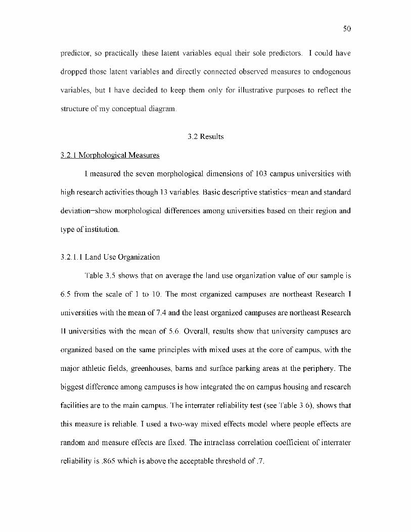
predictor, so practically these latent variables equal their sole predictors. I could have
dropped those latent variables and directly connected observed measures to endogenous
variables, but I have decided to keep them only for illustrative purposes to reflect the
structure of my conceptual diagram.
3.2 Results
3.2.1 Morphological Measures
I measured the seven morphological dimensions of 103 campus universities with
high research activities though 13 variables. Basic descriptive statistics-mean and standard
deviation-show morphological differences among universities based on their region and
type of institution.
3.2.1.1 Land Use Organization
Table 3.5 shows that on average the land use organization value of our sample is
6.5 from the scale of 1 to 10. The most organized campuses are northeast Research I
universities with the mean of 7.4 and the least organized campuses are northeast Research
II universities with the mean of 5.6. Overall, results show that university campuses are
organized based on the same principles with mixed uses at the core of campus, with the
major athletic fields, greenhouses, barns and surface parking areas at the periphery. The
biggest difference among campuses is how integrated the on campus housing and research
facilities are to the main campus. The interrater reliability test (see Table 3.6), shows that
this measure is reliable. I used a two-way mixed effects model where people effects are
random and measure effects are fixed. The intraclass correlation coefficient of interrater
reliability is .865 which is above the acceptable threshold of .7.
50

3.2.1.2 Compactness
Table 3.7 shows that on average the mass-space proportion of campuses is 1 to 4.
In other words, around 20% of campus grounds are covered with buildings. In addition, on
average, around 10% of campus grounds are covered with surface parking areas; 24% of
campus grounds are covered with pervious open spaces; and the average nearest distance
between campus buildings is 236.90 feet.
Table 3.7 also indicates that the Research I universities at Northeast region have
the densest campuses with around 25% mass density, 193 ft. building proximity, and less
than 6% surface parking areas. The Research II universities at South region are the most
sprawling campuses with around 17% mass density, 281 ft. building proximity, and 14.5%
surface parking areas. The Northeast Research II universities have the largest percentage
of pervious open spaces with 33% and the West Research II universities have the smallest
percentage of pervious open spaces with 15%.
3.2.1.3 Connectivity
Table 3.8 shows that on average campus connectivity (the local integration value
of campus street network weighted by segment length) is .3. There are major differences
among universities in regard to this dimension. While the average campus connectivity is
only .11 for South Research II universities with a small standard deviation of .07, the
average of campus connectivity for Northeast Research I universities is .5 with a large
standard deviation of .97. These differences can be explained by the type of urbanism at
each region. Campuses in more sprawling cities tend to have less street connectivity.
Campus connectivity relative to county connectivity is a measure of how integrated
the campus street network is to its county. A value of more than one indicates that the
51
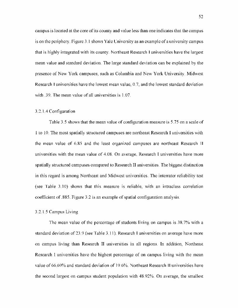
campus is located at the core of its county and value less than one indicates that the campus
is on the periphery. Figure 3.1 shows Yale University as an example of a university campus
that is highly integrated with its county. Northeast Research I universities have the largest
mean value and standard deviation. The large standard deviation can be explained by the
presence of New York campuses, such as Columbia and New York University. Midwest
Research I universities have the lowest mean value, 0.7, and the lowest standard deviation
with .39. The mean value of all universities is 1.07.
3.2.1.4 Configuration
Table 3.5 shows that the mean value of configuration measure is 5.75 on a scale of
1 to 10. The most spatially structured campuses are northeast Research I universities with
the mean value of 6.85 and the least organized campuses are northeast Research II
universities with the mean value of 4.08. On average, Research I universities have more
spatially structured campuses compared to Research II universities. The biggest distinction
in this regard is among Northeast and Midwest universities. The interrater reliability test
(see Table 3.10) shows that this measure is reliable, with an intraclass correlation
coefficient of .885. Figure 3.2 is an example of spatial configuration analysis.
3.2.1.5 Campus Living
The mean value of the percentage of students living on campus is 38.7% with a
standard deviation of 23.9 (see Table 3.11). Research I universities on average have more
on campus living than Research II universities in all regions. In addition, Northeast
Research I universities have the highest percentage of on campus living with the mean
value of 66.69% and standard deviation of 19.6%. Northeast Research II universities have
the second largest on campus student population with 48.92%. On average, the smallest
52

percentage of campus living is at West Research II universities with only 20.5% and the
standard deviation of 12.9%. South Research II universities have the second lowest
percentage of on campus living with 26.36% and standard deviation of 18.9%.
3.2.1.6 Greenness
Greenness dimension has three indicators: the percentage of tree canopy, the
percentage of pervious open spaces, and the percentage of parking surface areas. The last
two indicators are shared and discussed with the compactness dimension.
Table 3.12 shows that on average 13.7% of campus grounds are covered by tree
canopy. Northeast Research II universities have the highest average of tree canopy with
21.5%. Overall, campuses located at Northeast and South regions are more covered with
tree canopy than Midwest and West campuses. West Research II universities have the
lowest average percentage of tree canopy of only 6% with standard deviation of 4%.
3.2.1.7 Context
Table 3.13 shows that on average census tracts surrounding campuses have an
activity density of 12,5786, with land use entropy of .74, and intersection density of 110.
Activity density and intersection density vary substantially among regions, but not so much
in terms of land use entropy. Northeast universities have the highest activity density and
intersection density surrounding their campuses. South Research II universities have the
lowest activity and intersection densities. On average, South Research II universities have
the activity density of 4,213 with a standard deviation of 2,420, and an intersection density
53
6 The total population and employment per square mile.

54
of 70 with standard deviation of 35. Although entropy does not show substantial variation
among regions and university types, it is positively correlated with activity density and
intersection density at the significance level of .05.
3.2.2 Modeling Campus Form
The interaction among different morphological variables of university campuses
has not been explored in prior studies. I used Structural Equation Modeling software, Amos
22, to model campus morphological dimensions with the observed variables described at
Table 3.2. I created latent variables to represent morphological dimensions based on the
proposed hypothesis. I had to slightly modify my original hypothesis, to generate the best
model (in terms of goodness of fit indices and the significance of coefficient estimates).
First, I had to drop the proximity variable, because it did not show significant interaction
with other compactness variables. Second, I found significant interaction among
compactness, connectivity, and context dimensions. Instead of creating three distinct latent
variables, all related observed variables can be loaded on a broader latent variable that can
represent the degree of urbanism of campus. The other option that I had was creating a
second order latent variable of urbanism based on the three latent variables of compactness,
connectivity, and context. However, the first option- directly loading observed variables
on the urbanism latent variable-had a better model fit.
Some latent variables, such as campus living, have only one predictor, so practically
these latent variables equal their sole predictors. I could have dropped those latent variables
and directly correlated observed measures with the other latent variables, but I decided to
keep them only for illustrative purposes to show the clear structure of my conceptual
diagram.

Figure 3.3 shows the path diagram of my proposed hypothesis.7 On the left side,
the interaction of all dimensions is presented. However, I found no significant interaction
between two morphological dimensions and any of the outcome variables (which will be
discussed in the next sections). These two dimensions are the two qualitatively rated
dimensions: configuration and land use organization. Therefore, I have decided to model
campus form without these two dimensions. On the right side of Figure 3.3, the path
diagram of the remaining three latent variables is presented.
I used maximum likelihood procedures for estimation and to evaluate model
goodness-of-fit. Because of the relatively small number of sampled universities, I also
conducted Bayesian estimates (Riginos & Grace, 2008) using Amos for confirmatory
purposes, since these estimates do not depend on large-sample theory. This model
generates a good model fit by maximum likelihood estimation, but only gets a good model
fit with Bayesian estimates when the outliers were removed from the sample.8
The following results were obtained by removing outliers: The structural equation
model obtained through maximum likelihood estimation had 29 degrees of freedom and a
X2 value of 18.80 with a P value of 0.926. This P value along with all model fit indicators
(CFI is 1 and RMSEA is .000) indicate good model fit. In Bayesian estimation, the
Posterior Predictive P value has to be close to 0.5 to have a good model fit. This model had
the Posterior Predictive P value of 0.51, which indicates good model fit.
7 Dropping the correlations among error terms changes the coefficients very little, and does not change their signs and the significance levels of campus form variables; however, decreases the goodness of fit of the model. Chi-square= 29.119, Degrees of freedom=31, Probability level= .5638 Seven cases had leverage value more than 2: Columbia University, Temple University, Fordham University, Boston University, Brandeis University, New York University, and Miami University.
55

Table 3.14 shows the regression weights in maximum likelihood and Bayesian
estimation, P value of maximum likelihood estimates and 95% credible intervals for
Bayesian estimates. All regression paths possessed coefficients with significance level of
0.05 or beyond in both maximum likelihood and Bayesian estimations. Coefficient
estimates were close to each other with both techniques, which confirm the model. In
addition, the signs of coefficients were in accordance with the hypothesis. For example,
the percentage of pervious open space was positively loaded on greenness and negatively
loaded on urbanism. Also, the percentage of surface parking areas is negatively loaded on
both greenness and urbanism latent variables. The degree of campus living was positively
correlated with the degree of greenness at the significance level of <.001 (Figure 3.4). The
degree o f urbanism was negatively correlated with the degree o f greenness at the
significance level of <.001, which means more urbanized campuses are generally less green
(Figure 3.5). The degree of campus living and urbanism were not correlated (Figure 3.6).
3.2.3 Students’ Satisfaction, Learning Outcome, and Campus Form
After modeling campus form through three distinct latent variables, I investigated
the relationship between campus form, students’ satisfaction and learning outcomes. Figure
3.7 shows the path diagram of my model. The three latent variables, the degree of urbanism,
greenness and campus living, were generated from 10 observed variables, according to the
confirmed model in the previous step. Similar to the previous step, I used the marker-
variable strategy to specify the scale of latent variables based on one observed variable.
The latent variables are fixed to have means of 0, but their variances are not fixed.
The hypothesis is that the morphological dimensions (latent variables) can have
direct impacts on students’ satisfaction with their college experience and their overall
56
academic performance (learning outcomes). Also, students’ satisfaction with their college
experience can have a direct impact on their learning outcomes. I considered four control
variables for this model: (1) the total number of undergraduate enrollment to control for
the size of university; (2) the average SAT score to control for the student selectivity of
university; (3) the percentage of classes with fewer than 20 students to control for the
faculty resources of university; (4) the Research I or Research II university dummy variable
to control for the level of research activities. I also tested other control variables, such as
enrollment profile, university type (private or public), climate, crime rate, and the average
total indebtedness of graduates, but they had no significant impact on either endogenous
variables. In addition, I assumed that the exogenous variables are not orthogonal.
Therefore, I estimated the covariance between all exogenous variables.
Because my sample size is relatively small, similar to the previous step, I estimated
my model with both maximum likelihood and Bayesian estimations to support my
conclusions. The structural equation model obtained through maximum likelihood
estimation had 71 degrees of freedom and a x2 value of 70.206 with a P value of 0.504.
This P value along with all model fit indicators (CFI is 1 and RMSEA is .000) indicate
good model fit. The structural equation model obtained through Bayesian estimation had
the Posterior Predictive P value of 0.45, which indicates good model fit as well.
Table 3.15 shows the direct regression weights with both maximum likelihood and
Bayesian estimations. The results show that all three campus form variables have
significant positive correlation with freshman retention rate. To the best of my knowledge,
this is the first time that a significant correlation between the morphology of university
campuses and students’ satisfaction has been reported. One unit increase in the urbanism
57

latent variable (with the range of 1.90), is associated with the increase of the freshman
retention by 4.8%. One unit increase in the greenness latent variable (with the range of
37.75) is associated with the increase of the freshman retention by 0.2%. Also, 1% increase
in on campus residents is associated with the increase o f freshman retention by almost
0.1%. Note that even 1% increase of freshman retention rate is an important impact,
considering the fact that it may change the future of 200 people per year in a university
with 20,000 students.
All other control variables have significant correlation with freshman retention rate
as well in both maximum likelihood and Bayesian estimations. Studying at a Research I
university (with very high research activities) can have positive impact on students’
satisfaction compared to being a student at a Research II university (with high research
activities). Studying at a Research II university instead of Research I university is
associated with the decrease of the freshman retention about 2.8%. In addition, universities
which are more selective in giving admission have more chance to have higher freshman
retention rate. One hundred points more on the average of SAT score is associated with the
increase of the freshman retention rates 4.6%. The number of undergraduate students can
also have significant positive correlation. However, it requires 10,000 more undergraduate
enrollments to increase freshman retention only 1.6%. The percentage of classes with less
than 20 students had significant negative correlation with freshman retention rate. Ten
percent increase in the number o f classes with less than 20 students can decrease freshman
retention by 1.35%. This result may be explained by the fact that universities with smaller
classes tend to have a more rigorous education system and, therefore, to be more
58

demanding academically. This may cause students with lower academic abilities to drop
out of school after their freshman year.
The impact of the freshman retention rate on the 6-year graduation rate is very
strong and significant. One percent increase for freshman retention can increase the 6-year
graduation rate by 1.355% increase. Since all variables (3 latent variables and 4 control
variables) showed significant impact on the freshman retention rate, and the freshman
retention rate has a significant impact on the 6-year graduation rate, we can conclude that
all variables have a significant indirect impact on 6-year graduation rate. However, only
two variables (greenness, and campus living) other than freshman retention rate show a
significant direct impact on 6-year graduation rate. The total standardized effect of campus
living on the graduation rate is .315 and the total standardized effect of greenness is .292
(see Figure 3.16). Ten percent increase of on campus residents is associated with the
increase of the 6-year graduation rate by 2.43%, considering both direct and indirect
effects. Also, a 10-unit increase in the greenness measure is associated with the increase of
the 6-year graduation rate by 5.58%, again considering both direct and indirect effects.
3.2.4 Campus Score
In order to rank universities based on the quality of their campuses, I developed a
composite score from the three latent variable of urbanism, greenness, and campus living.
First, I standardized these three latent variables with the mean of 0 and the standard
deviation of 1. The composite score is generated with the following formula:
Score= .177XUrban+.215 XGreen+.251 X Living
59
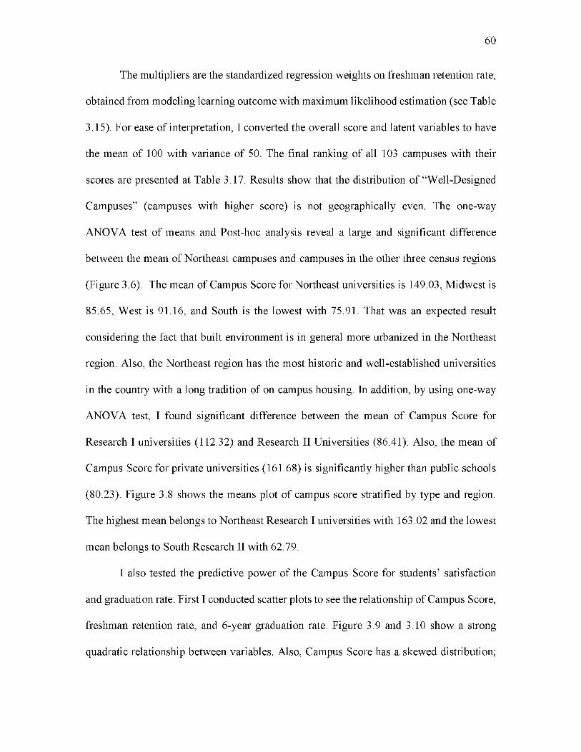
The multipliers are the standardized regression weights on freshman retention rate,
obtained from modeling learning outcome with maximum likelihood estimation (see Table
3.15). For ease of interpretation, I converted the overall score and latent variables to have
the mean of 100 with variance of 50. The final ranking of all 103 campuses with their
scores are presented at Table 3.17. Results show that the distribution of “Well-Designed
Campuses” (campuses with higher score) is not geographically even. The one-way
ANOVA test of means and Post-hoc analysis reveal a large and significant difference
between the mean of Northeast campuses and campuses in the other three census regions
(Figure 3.6). The mean of Campus Score for Northeast universities is 149.03, Midwest is
85.65, West is 91.16, and South is the lowest with 75.91. That was an expected result
considering the fact that built environment is in general more urbanized in the Northeast
region. Also, the Northeast region has the most historic and well-established universities
in the country with a long tradition of on campus housing. In addition, by using one-way
ANOVA test, I found significant difference between the mean of Campus Score for
Research I universities (112.32) and Research II Universities (86.41). Also, the mean of
Campus Score for private universities (161.68) is significantly higher than public schools
(80.23). Figure 3.8 shows the means plot of campus score stratified by type and region.
The highest mean belongs to Northeast Research I universities with 163.02 and the lowest
mean belongs to South Research II with 62.79.
I also tested the predictive power of the Campus Score for students’ satisfaction
and graduation rate. First I conducted scatter plots to see the relationship of Campus Score,
freshman retention rate, and 6-year graduation rate. Figure 3.9 and 3.10 show a strong
quadratic relationship between variables. Also, Campus Score has a skewed distribution;
60

therefore I conducted natural log transformation on Campus Score, before exploring its
predictive power.
I conducted two linear regression analyses. First, I modeled the freshman retention
rate with the natural log transformed Campus Score, average SAT score, the percentage of
classes with less than 20 students, university type (Research I or II), and the total number
of undergraduates.9 Second, I modeled the 6-year graduation rate with the freshman
retention rate and the natural log transformed Campus Score. None of the other control
variables was significant in this model. No multicollinearity nor outlier impact has been
detected in these models.
The first model had the adjusted R2 of 0.802, and all coefficient estimates were at
the significance level of 0.05 or beyond. The general findings were consistent with the
SEM model. The difference was having a single composite variable instead of using three
distinct latent variables in the model. The unstandardized coefficient of Campus Score was
6.893, and the standardized coefficient was 0.414. This means 1% increase in Campus
Score can increase the freshman retention rate by 0.0689.
The second model had the adjusted R2 of 0.917, and all coefficient estimates were
at the significance level of less than .001. The unstandardized coefficient of the freshman
retention rate was 1.483 and standardized coefficient was .745. The unstandardized
coefficient of the natural log transformed Campus Score was 8.989 and standardized
coefficient was .271. This means 1% increase in Campus Score can increase the 6-year
graduation rate by 0.0899.
61
9 Same control variables as the SEM model

3.2.5 Campus Safety and Campus Form
I also investigated the relationship between campus form and campus crime. Figure
3.11 shows the path diagram of my model. Similar to the previous steps, I used the three
latent variables, the degree o f urbanism, greenness and campus living, to represent campus
morphological dimensions. The hypothesis is that the morphological dimensions can have
impact on campus crime rate after controlling for the following variables: (1) the
percentage o f undergraduate students from the total enrollment to control for the academic
profile of university; (2) the average SAT score to control for the student selectivity of
university; (3) the percentage of classes with fewer than 20 students to control for the
faculty resources o f university; (4) the median income o f city to control for the socio
economic status of city; (5) the sum of total cooling and heating days in city to control for
climate. I also tested other control variables, such as university type (private or public),
crime rate of city, research type and the average total indebtedness of graduates, but they
had no significant impact on the endogenous variable. Similar to the previous models, I
assumed that the exogenous variables are not orthogonal, and I estimated the covariance
between all exogenous variables.
Similar to the previous steps, I estimated my model with both maximum likelihood
and Bayesian estimations to support my conclusions. The structural equation model
obtained through maximum likelihood estimation had 71 degrees of freedom and a x2 value
of 68.173 with a P value of 0.573. This P value along with all model fit indicators (CFI is
1 and RMSEA is .000) indicate good model fit. The structural equation model obtained
through Bayesian estimation had the Posterior Predictive P value of 0.51, which indicates
good model fit.
62

Table 3.18 shows the regression weights with both maximum likelihood and
Bayesian estimations. The results show that the degree of urbanism and greenness are
negatively correlated with the crime rate. However, the coefficient estimate of greenness
is not significant at .05 level. One unit degree increase in urbanism (with the range of 1.9)
can decrease the campus crime rate by 5.671 units (the number of criminal offenses per
10,000 students is the unit). The third morphological variable, campus living, is positively
correlated with campus crime rate at the 0.05 significance level. One unit increase in the
percentage of on campus living can increase the campus crime rate by 0.063. This is not a
very strong impact, since it requires 16% increase on campus residents to only change one
unit of campus crime rate.
All control variables had significant correlation with the campus crime rate. A ten
thousand dollar increase in the median income of households in the city can increase the
crime rate by 0.53. Also, 100-point increase on the average of SAT score can decrease the
crime rate 0.9. In other words, being more selective on admissions means less crime on
campus. One unit increase on the percentage of undergraduate students can decrease crime
rate -0.105. One unit increase in the percentage of classes with less than 20 students can
increase crime rate by .086. The last two facts are suggesting that universities with high
graduate/professional students and smaller classes have higher crime rates. This result,
which is to some extent unexpected, can be explained by the fact that universities with
small classes and high portion of graduate students normally have fewer students;
therefore, although they may have less crime on their campus, they can have more crimes
per capita. In addition, although the victims are generally affiliated with the university, not
all offenders necessarily are. Finally, 1,000 units increase in the climate index (with the
63

rage of 10,500) can decrease crime rate by 1 unit. This is an interesting finding to know
that there are higher crime rates at campuses with moderate climates than severe climates.
This can be explained by the fact that students in moderate climates are outside more and
therefore have more exposure to crime.
I also tested the predictive power of the Campus Score (generated at section 3.2.4)
on campus crime using a linear regression. The results showed that the Campus Score has
no significant correlation with campus crime rate, considering other control variables. This
was an expected result, since the three latent variables had different signs of correlation
with campus crime rate.
3.2.6 Campus Sustainability and Campus Form
Sustainability is a very broad concept. Therefore, defining sustainable campus form
can be a multifaceted and exceptionally complex task. One of the most comprehensive
attempts to assess and rate sustainability for university campuses has been done by the
Association for the Advancement of Sustainability in Higher Education (AASHE), known
as the Sustainability Tracking, Assessment & Rating System™ (STARS). I investigated
the predictive power of campus form (as measured in this research) on the sustainability
ratings of STARS.
From my 103 campus sample, 61 universities (59.2%) have participated in STARS
program and have unexpired ratings. Twenty-eight campuses have Gold ratings, 31 have
Silver ratings, and only 2 campuses have Bronze ratings. I created a dummy variable with
1 equals Gold and 0 equals non-Gold ratings. The total sample has 40.8% missing values.
When missing values are present, it is essential to estimate means and intercepts (which is
not the default in Amos). Amos uses full information maximum likelihood (FIML)
64

estimation which requires using all information of the observed data unlike listwise or
pairwise deletion methods.10 In Amos, modeling binary outcome variables requires the use
of Markov Chain Monte Carlo (MCMC) option. In addition, Amos uses a probit model for
ordered-categorical outcomes. This means regression weights specify the effect of one unit
change in the exogenous variables on the probability of observing 1 for the outcome
variable.
I tested the interaction among the three morphological latent variables (the degree
of urbanism, greenness and campus living) with the STARS ratings. I did not detect any
significant correlation between the campus form measures and STARS rating. I also did
not detect any significant correlation between other variables, such as the climate index,
university type, or enrollment profile with STARS. In SPSS, I also used a binary logistic
model with the Campus Score as the predictive variable; but I found no significant
interaction between the Campus Score and STARS rating. STARS has a very complex
credit checklist and it is heavily weighted toward sustainability programs and policies of
universities. STARS credit checklist is organized under the four categories of (1)
academics, (2) engagement, (3) operations, and (4) planning and administration with 18
subcategories.11
Another explanation can be that university programs and policies regarding
sustainability do not necessarily correlate with the sustainability of the physical campus.
In order to test the impact of campus form on sustainability issues it is better to be more
10 See FIML estimation by Jim Arbuckle in the edited volume by Marcoulides and Schumacker (2013)
11 See STARS 2.0 Credit Checklist at:http://www.aashe.org/files/documents/STARS/2.0/stars 2.0 credit checklist 1.pdf
65

specific about defining sustainability. Therefore, in the next section, I investigate the
impact o f campus form on the commuting behaviors o f students and staff as one aspect o f
sustainability.
3.2.7 Students’ Commuting Behavior and Campus Form
Figure 3.12 shows the path diagram of my model. The hypothesis is that the
morphological dimensions can have impact on students’ commuting behavior after
controlling for the following variables: (1) the urbanism degree of setting; (2) the
enrollment profile classification; and (3) the university type. This model had three
endogenous variables (the percentage o f students who walk or bike, the percentage o f
students who commute with only the driver in the vehicle, and the percentage o f students
who take a campus shuttle or public transportation as their primary method o f
transportation) that are highly correlated; therefore, their covariances were estimated. Note
that the sum of these three variables is not necessarily 100%. For example, those who
carpool were not included in any o f these categories. These data are self-reported data by
institution from STARS. Therefore, the issue of missing data applies for these data as well.
The missing values are 30% of all cases. However, because Amos uses full information
maximum likelihood (FIML), all 103 cases contribute information to the model.
I estimated my model with both maximum likelihood and Bayesian estimations.
The structural equation model obtained through maximum likelihood estimation had 71
degrees of freedom and a x2 value of 71.792 with a P value of 0.451. This P value along
with all model fit indicators (CFI is 0.999 and RMSEA is .010) indicate good model fit.
The structural equation model obtained through Bayesian estimation had the Posterior
Predictive P value of perfect 0.5, which indicates good model fit.
66

Table 3.19 shows the regression weights with both maximum likelihood and
Bayesian estimations. The results of both estimations show that the only correlated variable
(at the 0.05 significance level) with the percentage o f students who walk or bike is the
percentage o f on campus residents. One unit change in the percentage o f campus residents
can increase the outcome variable by 0.336. With maximum likelihood estimation, all
exogenous variables are correlated with the percentage o f students who commute with only
the driver in the vehicle at the 0.05 significance level, except for the enrollment profile.
However, Bayesian estimation just confirmed the significance of three estimates: the
degree o f urbanism o f campus, the degree o f greenness, and the university type.
One unit change in the urbanism degree (with the range of 1.9) can decrease the
percentage of students who drive alone by 24.068. The relationship between car usage and
campus greenness can be hypothesized in both causal ways: Either less use o f cars by
students can make campus greener, or greener campuses can encourage students to use less
cars. I assumed the latter in my model. One unit change in the greenness degree (with the
range of 37.75) can decrease the percentage of students who drive alone by 1.055, which
is also very substantial. In addition, being at a Research II university instead of Research I
university can increase the percentage of students who drive alone by 12.5.
The degree o f urbanism and the degree o f greenness have significant positive
impact on the percentage of students using transit. One unit change in the urbanism degree
can increase the percentage of students using transit by 27.702. One unit change in the
greenness degree can increase the same percentage by .883. In the maximum likelihood
estimation, the degree of urbanism of setting showed significant positive correlation with
67

the percentage of students who use transit. However, the Bayesian estimation did not
confirm the significance of this correlation at the 0.05 level.
3.2.8 Employees’ Commuting Behavior and Campus Form
Figure 3.13 shows the path diagram of employees’ commuting behavior as a
function of morphological measures of campus design, considering these control variables:
(1) the urbanism degree of setting; (2) the enrollment profile classification; and (3) the
university type. This model also had three endogenous variables (the percentage of
employees who walk or bike, the percentage of employees who commute with only the
driver in the vehicle, and the percentage of employees who take a campus shuttle or public
transportation as their primary method of transportation). This information was not
available for 33% of cases.
The structural equation model obtained through maximum likelihood estimation
had 71 degrees of freedom and a x2 value of 72.544 with a P value of 0.427. This P value
along with all model fit indicators (CFI is 0.998 and RMSEA is .015) indicate good model
fit. The structural equation model obtained through Bayesian estimation had the Posterior
Predictive P value of perfect 0.5, which indicates good model fit.
Table 3.20 shows the regression weights with both maximum likelihood and
Bayesian estimations. The results of both estimations showed that none of the three
morphological measures had a significant correlation with the percentage o f employees
who walk or bike. However, both estimations showed significant negative correlation
between the urbanism degree of campus and the percentage o f employees who commute
with only the driver in the vehicle at the 0.05 significance level. One unit increase in the
urbanism degree can decrease the percentage of employee who drive alone by 34.545 units.
68

Also, working at a Research II institution instead of a Research I can increase the
percentage of employees who drive alone by 13.29%. This finding can be explained by the
fact that Research I universities (which generally have more financial resources) may have
invested more on the alternative transit modes, such as expanding their shuttle bus service,
or master planning bicycle routes. In addition, the degree of urbanism and the degree of
greenness of campus have significant positive impacts on the percentage of employees
using transit. One unit increase in the urbanism latent variable can increase the percentage
of employees using transit by 40.684. Also, one unit change in the greenness latent variable
can increase that same percentage by .688.
69
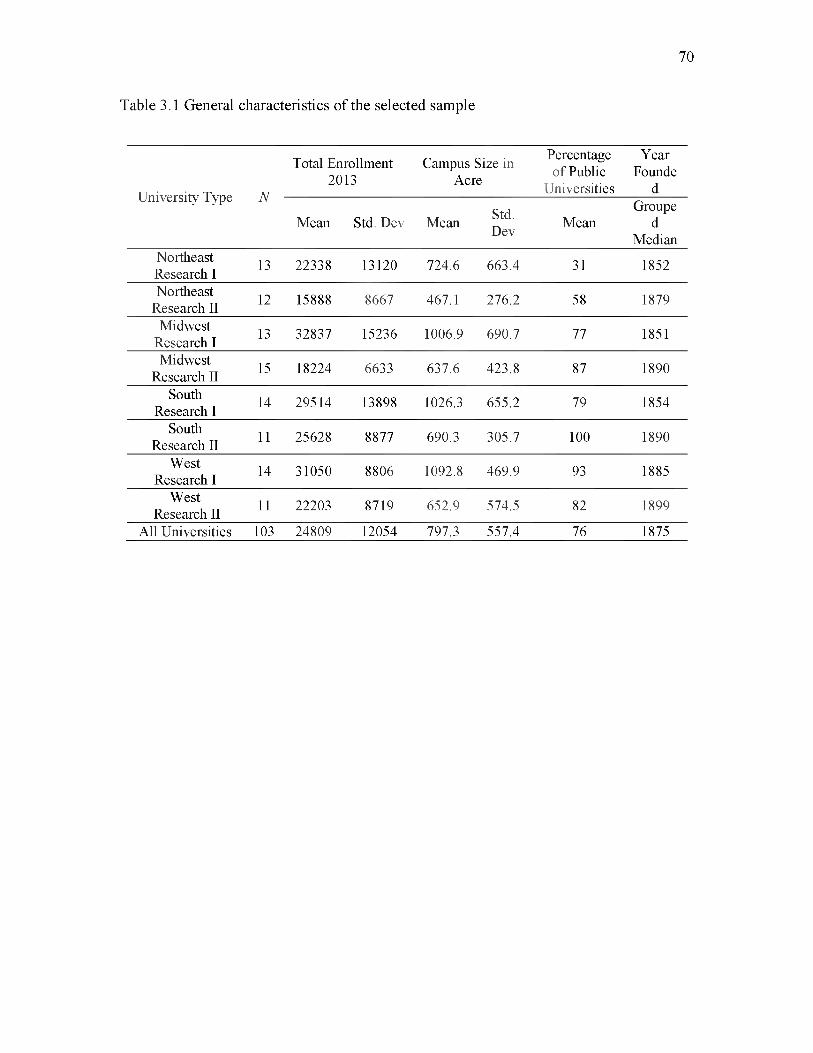
70
Table 3.1 General characteristics of the selected sample
Total Enrollment 2013
Campus Size in Acre
Percentage of Public
YearFounde
University Type N Universities d
Mean Std. Dev Mean Std.Dev Mean
Grouped
MedianNortheast Research I 13 22338 13120 724.6 663.4 31 1852
Northeast Research II 12 15888 8667 467.1 276.2 58 1879
Midwest Research I 13 32837 15236 1006.9 690.7 77 1851
Midwest Research II 15 18224 6633 637.6 423.8 87 1890
South Research I 14 29514 13898 1026.3 655.2 79 1854
South Research II 11 25628 8877 690.3 305.7 100 1890
West Research I 14 31050 8806 1092.8 469.9 93 1885
West Research II 11 22203 8719 652.9 574.5 82 1899
All Universities 103 24809 12054 797.3 557.4 76 1875
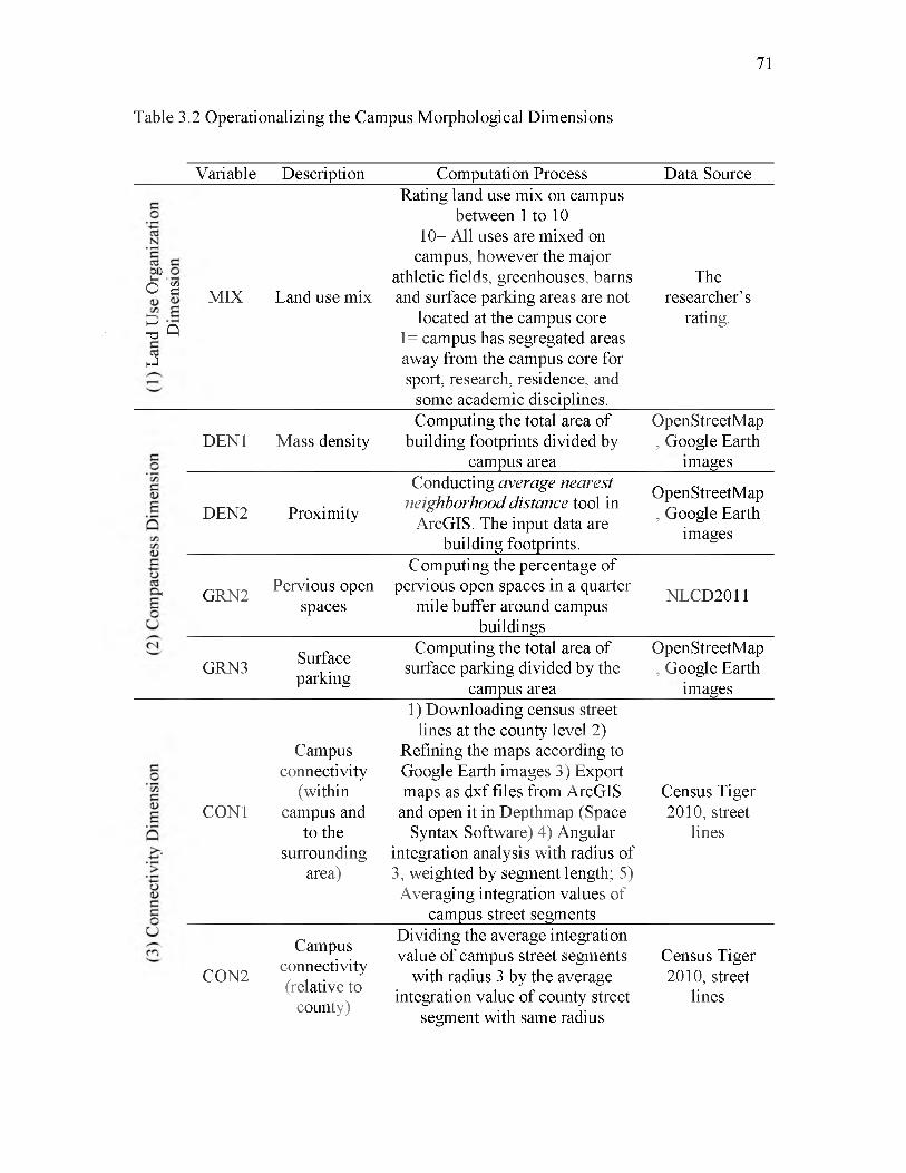
71
Table 3.2 Operationalizing the Campus Morphological Dimensions
Variable Description________ Computation Process_________ Data Source
noi
Rating land use mix on campus between 1 to 10tia
iznia ng o
O £e e
£ QnahJ
10= All uses are mixed on
MIX Land use mix
campus, however the major athletic fields, greenhouses, barns and surface parking areas are not
Theresearcher’s
located at the campus core 1= campus has segregated areas away from the campus core for sport, research, residence, and
some academic disciplines.
rating.
nioDEN1 Mass density
Computing the total area o f building footprints divided by
OpenStreetMap , Google Earth
campus area imagesisneimeDisse
DEN2 Proximity
Conducting average nearest neighborhood distance tool in
ArcGIS. The input data are building footprints.
OpenStreetMap , Google Earth
imagesntcapmoC
GRN2 Pervious open spaces
Computing the percentage o f pervious open spaces in a quarter
mile buffer around campus buildings
NLCD2011
(2)
GRN3 Surfaceparking
Computing the total area o f surface parking divided by the
OpenStreetMap , Google Earth
campus area images
niosineimDi
viiticenno
CON1
Campus connectivity
(within campus and
to the surrounding
area)
1) Downloading census street lines at the county level 2)
Refining the maps according to Google Earth images 3) Export maps as dxf files from ArcGIS
and open it in Depthmap (Space Syntax Software) 4) Angular
integration analysis with radius o f 3, weighted by segment length; 5) Averaging integration values o f
Census Tiger 2010, street
lines
campus street segmentsC(3)
CON2
Campus connectivity (relative to
county)
Dividing the average integration value o f campus street segments
with radius 3 by the average integration value o f county street
segment with same radius
Census Tiger 2010, street
lines

72
Table 3.2 Continued
Variable Description Computation Process Data Source
niosine
no'Srugfi
noC
STRU campus spatial structure
Rating the strength of campus spatial structure from 1 to 10.
10= The entire campus has organized around most of these
principles: Buildings are defining open spaces. Campus spaces are connected through main corridors, courtyards, or
quads. Campus has a main central space such as a plaza or
a lawn, long view corridors with a land mark at the focal point, enclosed open spaces, and the entire master plan is
relatively symmetric and geometric.
1= The campus has a _____ disorganized layout._____
Theresearcher’s
rating.
g ni
s si a sE E a i
C D
INHB On campus Computing the percentage of living students living on campus
US News and World Report
se n C .2<U (U
O .E(o' ®
GRN1
GRN2
GRN3
tree canopy
Computing the average percentage of tree canopy in a
quarter mile buffer around campus buildings
Pervious open spaces12
NLCD2011
Described under compactness dimension
Surfaceparking13 Described under compactness dimension
12 “Pervious open spaces ” is a shared variable among greenness and compactness dimension, but with different loading sign. More pervious open space means more greenness, but less compactness.
13 “Surface parking’ is a shared variable among greenness and compactness dimension, with same loading sign. More surface parking areas means less greenness and compactness.
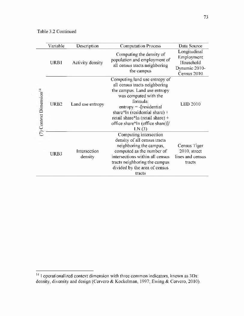
73
Table 3.2 Continued
Variable Description Computation Process Data Source
URB1 Activity density
Computing the density of population and employment of all census tracts neighboring
the campus
Longitudinal Employment Household
Dynamic 2010- Census 2010
URB2 Land use entropy
Computing land use entropy of all census tracts neighboring
the campus. Land use entropy was computed with the
formula: entropy = -[residential LED 2010
share*ln (residential share) + retail share*ln (retail share) + office share*ln (office share)]/
LN (3)
niosineme
xetnoC7)
URB3
Computing intersection density of all census tracts neighboring the campus,
Intersection computed as the number ofdensity intersections within all census
tracts neighboring the campus divided by the area of census
tracts
Census Tiger 2010, street
lines and census tracts
14 I operationalized context dimension with three common indicators, known as 3Ds: density, diversity and design (Cervero & Kockelman, 1997; Ewing & Cervero, 2010).

74
Table 3.3 Endogenous variables and their data source
Variable Proxy Variable Data Source
Student satisfaction with college experience
freshmen retention rate CollegeNavigator
Learningoutcome
6-year graduation rate CollegeNavigator
The Campus
Safety Total criminal offenses on campus from 2011 to 2013, divided by total enrollments 2011-2013
Safety and Security Data Analysis Cutting Tool
Sustainability STAR scores
TheSustainability Tracking, Assessment & Rating System
The percentage of institution’s students who walk, bicycle, or use other nonmotorized means as their primary means of transportation.
Students’commutingbehavior
The percentage of institution’s students who commute with only the driver in the vehicle (excluding motorcycles and scooters) as their primary means of transportation.
The percentage of institution’s students who take a campus shuttle or public transportation as their primary means of transportation.
TheSustainabilityTracking,
The percentage of institution’s employees who walk, bicycle, or use other nonmotorized means as their primary means of transportation.
Assessment & Rating System
Employees’commutingbehavior
The percentage of institution’s employees who commute with only the driver in the vehicle (excluding motorcycles and scooters) as their primary means of transportation.
The percentage of institution’s employees who take a campus shuttle or public transportation as their primary means of transportation.
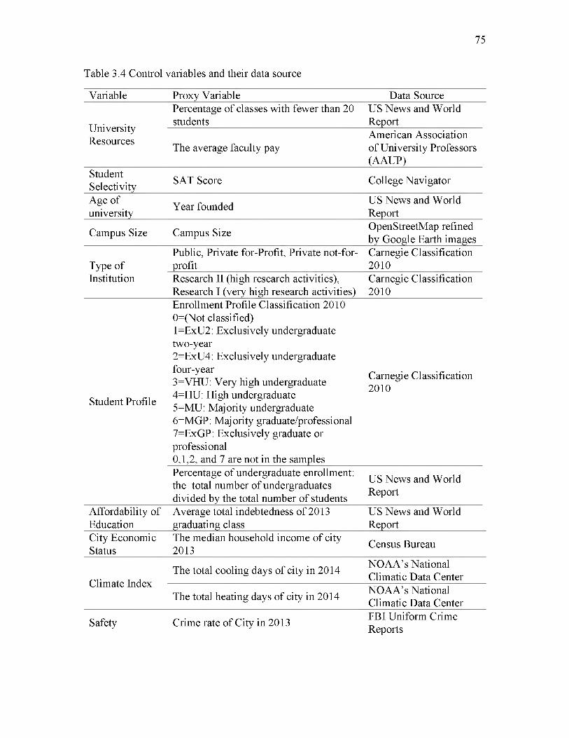
75
Table 3.4 Control variables and their data source
Variable Proxy Variable Data SourcePercentage of classes with fewer than 20 US News and World
UniversityResources
students ReportAmerican Association
The average faculty pay of University Professors (AAUP)
StudentSelectivity SAT Score College Navigator
Age of university Year founded US News and World
Report
Campus Size Campus Size OpenStreetMap refined by Google Earth images
Public, Private for-Profit, Private not-for- Carnegie ClassificationType of profit 2010Institution Research II (high research activities),
Research I (very high research activities)Carnegie Classification 2010
Enrollment Profile Classification 20100=(Not classified)1=ExU2: Exclusively undergraduate
Student Profile
two-year2=ExU4: Exclusively undergraduate four-year3=VHU: Very high undergraduate 4=HU: High undergraduate 5=MU: Majority undergraduate 6=MGP: Majority graduate/professional 7=ExGP: Exclusively graduate or professional0,1,2, and 7 are not in the samples
Carnegie Classification 2010
Percentage of undergraduate enrollment: the total number of undergraduates divided by the total number of students
US News and World Report
Affordability of Average total indebtedness of 2013 US News and WorldEducation graduating class ReportCity Economic Status
The median household income of city 2013 Census Bureau
Climate IndexThe total cooling days of city in 2014 NOAA’s National
Climatic Data Center
The total heating days of city in 2014 NOAA’s National Climatic Data Center
Safety Crime rate of City in 2013 FBI Uniform Crime Reports

76
Table 3.4 Continued
Variable Proxy Variable Data Source
The degree of urbanism of setting
4=City3=Suburban2=Town1=Rural
Carnegie Classification 2010
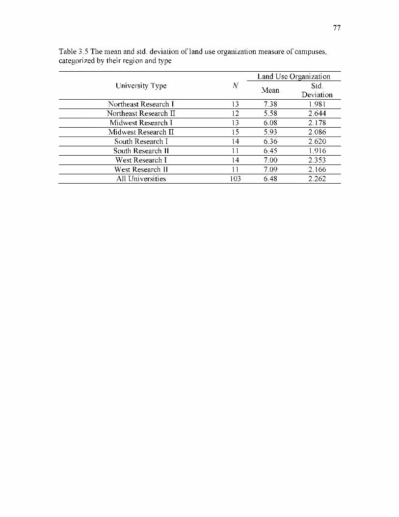
77
Table 3.5 The mean and std. deviation of land use organization measure of campuses,categorized by their region and type
Land Use OrganizationUniversity Type N Mean Std.
DeviationNortheast Research I 13 7.38 1.981Northeast Research II 12 5.58 2.644Midwest Research I 13 6.08 2.178Midwest Research II 15 5.93 2.086
South Research I 14 6.36 2.620South Research II 11 6.45 1.916West Research I 14 7.00 2.353West Research II 11 7.09 2.166All Universities 103 6.48 2.262
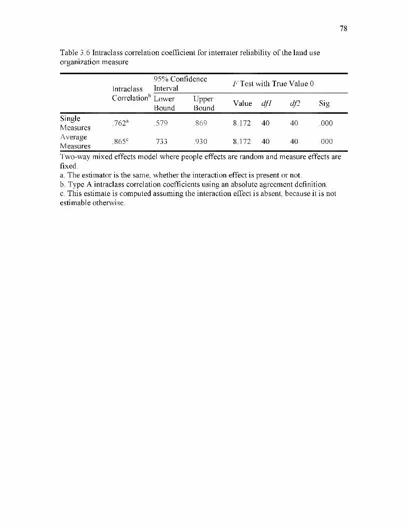
78
Table 3.6 Intraclass correlation coefficient for interrater reliability of the land use organization measure
Intraclass95% Confidence Interval F Test with True Value 0
Correlation13LowerBound
UpperBound Value df1 df2 Sig
SingleMeasures .762a .579 .869 8.172 40 40 .000
AverageMeasures .865c .733 .930 8.172 40 40 .000
Two-way mixed effects model where people effects are random and measure effects are fixed.a. The estimator is the same, whether the interaction effect is present or not.b. Type A intraclass correlation coefficients using an absolute agreement definition.c. This estimate is computed assuming the interaction effect is absent, because it is not estimable otherwise.

79
Table 3.7 The mean and std. deviation of compactness measures of universities,categorized by their region and type
University Type N
MassDensity
Proximity (in feet)
Percentage o f pervious open spaces
Percentage o f surface
parking area
Mean Std.D Mean Std.
D Mean Std.D Mean Std.
DNortheast Research I 13 .247 .128 193 59 28 21 5.96 3.87Northeast Research II 12 .201 .092 239 51 33 25 8.90 3.65Midwest Research I 13 .208 .079 253 48 19 15 8.45 3.13Midwest Research II 15 .180 .092 292 41 16 12 9.42 4.81
South Research I 14 .195 .067 205 51 27 20 10.36 4.29South Research II 11 .170 .053 234 59 29 15 14.42 6.26West Research I 14 .213 .055 198 44 27 10 11.25 4.57West Research II 11 .230 .065 281 95 15 11 13.42 5.60All Universities 103 .205 .083 236 65 24 17 10.14 5.06

80
Table 3.8 The mean and std. deviation of connectivity measures of universities,categorized by their region and type
University Type NCampus connectivity
Campus connectivity relative to county
connectivity
Mean Std.Deviation Mean Std.
DeviationNortheast Research I 13 .50 .97 1.56 1.75Northeast Research II 12 .41 .73 1.00 .90Midwest Research I 13 .39 .59 .70 .39Midwest Research II 15 .34 .39 .93 .92
South Research I 14 .14 .22 .87 .67South Research II 11 .11 .07 .99 .62West Research I 14 .19 .26 1.41 2.35West Research II 11 .27 .30 1.16 .67All Universities 103 .30 .52 1.07 1.21
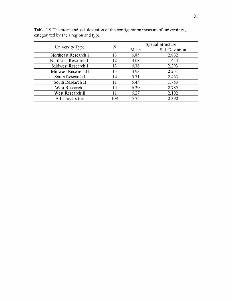
81
Table 3.9 The mean and std. deviation of the configuration measure of universities,categorized by their region and type
University Type N ■ Spatial StructureMean Std. Deviation
Northeast Research I 13 6.85 2.882Northeast Research II 12 4.08 1.443Midwest Research I 13 6.38 2.293Midwest Research II 15 4.93 2.251
South Research I 14 5.71 2.463South Research II 11 5.45 1.753West Research I 14 6.29 2.785West Research II 11 6.27 2.102All Universities 103 5.75 2.392

82
Table 3.10 Intraclass correlation coefficients for the configuration measure
Intraclass95% Confidence Interval F Test with True Value 0
Correlation13LowerBound
UpperBound Value df1 df2 Sig
SingleMeasures .793a .609 .890 10.042 40 40 .000
AverageMeasures .885c .757 .942 10.042 40 40 .000
Two-way mixed effects model where people effects are random and measure effects are fixed.a. The estimator is the same, whether the interaction effect is present or not.b. Type A intraclass correlation coefficients using an absolute agreement definition.c. This estimate is computed assuming the interaction effect is absent, because it is not estimable otherwise.

83
Table 3.11 The mean and std. deviation of campus living measure of universities,categorized by their region and type
University Type N Percentage of students Mean
living on campus Std. Deviation
Northeast Research I 13 66.69 19.653Northeast Research II 12 48.92 22.633Midwest Research I 13 38.23 26.768Midwest Research II 15 30.33 20.056
South Research I 14 40.29 20.398South Research II 11 26.36 18.917West Research I 14 33.14 19.159West Research II 915 20.56 12.943All Universities 101 38.70 23.915
15 Idaho State University and Portland State University were the missing data.

84
Table 3.12 The mean and std. deviation of campus living measure of universities,categorized by their region and type
University Type NThe average percentage o f tree
canopy Mean Std. Deviation
Northeast Research I 13 18.03 10.13Northeast Research II 12 21.48 16.11Midwest Research I 13 8.78 5.24Midwest Research II 15 10.33 8.56
South Research I 14 19.29 17.09South Research II 11 19.43 14.15West Research I 14 6.64 4.44West Research II 11 5.99 4.12All Universities 103 13.71 12.26

85
Table 3.13 The mean and std. deviation of campus living measure of universities,categorized by their region and type
University Type N Activity Density Entropy Intersection Density
Mean Std. D. Mean Std. D. Mean Std. D.Northeast Research I 13 21833 23045 .74 .14 132 90Northeast Research
II 12 17628 18723 .71 .18 138 125
Midwest Research I 13 12848 6428 .72 .11 131 32Midwest Research II 15 10275 9650 .76 .12 104 47
South Research I 14 10195 9196 .75 .12 108 50South Research II 11 4213 2420 .72 .11 70 35West Research I 14 9106 3507 .79 .06 98 34West Research II 11 14767 16168 .75 .13 99 50All Universities 103 12578 13479 .74 .12 110 66

86
Table 3.14 The regression weights (ML and Bayesian) in modeling campus form
Maximum Likelihood Bayesian
RegressionWeights
Pvalue
RegressionWeights
95%Lowerbound
95% Lower bound o f
GRN1 <— Green 1.000 1.000GRN3 <— Green -.286 .000 -.295 -0.467 -0.154GRN2 <— Green 1.149 .000 1.159 0.771 1.649CON1 <— Urban 1.000 1.000CON2 <— Urban .878 .020 1.050 0.271 1.845URB1 <— Urban 34.132 .000 37.117 27.220 51.123URB2 <— Urban .117 .048 .129 0.044 0.233URB3 <— Urban 150.570 .000 164.637 117.294 232.034DEN1 <— Urban 20.385 .000 22.356 16.391 30.852GRN3 <— Urban -10.127 .002 -11.241 -17.536 -6.538GRN2 <— Urban -15.798 .002 -17.271 -30.207 -5.286

87
Table 3.15 The regression weights (ML and Bayesian) in modeling students’ satisfaction and learning outcome16
Maximum Likelihood Bayesian
RegressionWeights
Standardized Regression P value
Weights
RegressionWeights
95%Lowerbound
95%Lowerbound
ofFRR <-- Urban 4.809 .177 .034 5.101 .393 10.877FRR <-- Green .206 .215 .023 .208 0.429 0.449FRR <-- Living .097 .251 .004 .097 0.026 0.167FRR <-- Research -2.773 -.151 .022 -2.827 -5.364 -0.339FRR <-- Faculty -.135 -.199 .005 -.134 -0.235 -0.034FRR <-- SAT .046 .629 *** .045 0.031 0.059FRR <-- UnderGr .162 .169 .015 .164 0.023 0.305
GRA6 <-- FRR 1.355 .068 *** 1.365 1.084 1.640GRA6 <-- Urban 3.662 .146 .210 3.848 -2.415 11.651GRA6 <-- Green .278 .144 .023 .276 0.022 0.583GRA6 <-- Living .111 .007 .010 .111 0.018 0.203GRA6 <-- SAT .017 .036 .094 .016 -0.004 0.037GRA6 <-- Research .252 .116 .871 .281 -3.012 3.494GRA6 <-- Faculty .048 .078 .442 .051 -0.085 0.180GRA6 <-- UnderGr .148 .681 .082 .152 -0.027 0.335
16 Dropping the covariates/control variables increases the coefficients, but does not change their signs and the significance levels of campus form variables. The coefficient estimates would be: Urban -> FRR: 9.764; Green -> FRR .376; Living -> FRR .168; Urban ->4.50; Green -> GRA6: .285; Living -> GRA6: .106.

88
Table 3.16 The total effects of exogenous variables on 6-year graduation rate.
Maximum Likelihood Bayesian
Total Effects Standardized Total Effects
TotalEffects
Standardized Total Effects
Urban 10.181 .189 10.754 .189Green .558 .292 .558 .291Living .243 .315 .245 .315
Research -3.507 -.096 -3.575 -.098Faculty -.135 -.100 -.132 -.097
SAT .078 .544 .078 .542UnderGr .367 .193 .377 .198
FRR 1.355 .681 1.365 .685
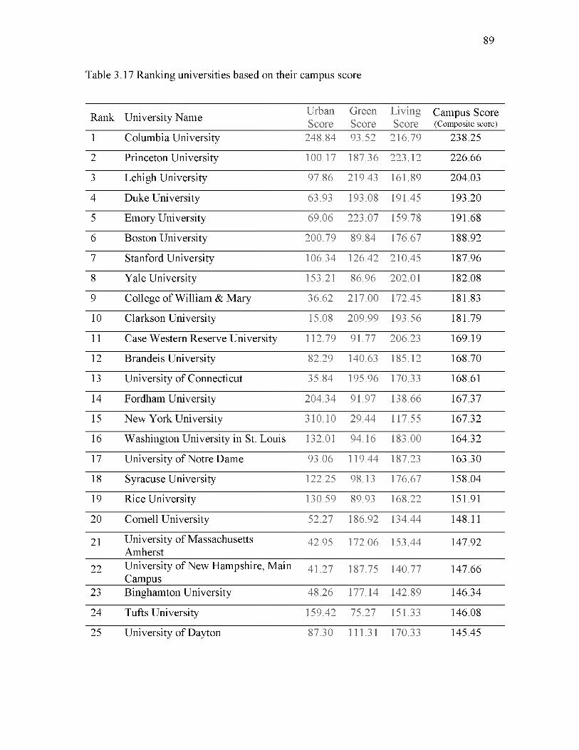
89
Table 3.17 Ranking universities based on their campus score
Rank University Name UrbanScore
GreenScore
LivingScore
Campus Score(Composite score)
1 Columbia University 248.84 93.52 216.79 238.25
2 Princeton University 100.17 187.36 223.12 226.66
3 Lehigh University 97.86 219.43 161.89 204.03
4 Duke University 63.93 193.08 191.45 193.20
5 Emory University 69.06 223.07 159.78 191.68
6 Boston University 200.79 89.84 176.67 188.92
7 Stanford University 106.34 126.42 210.45 187.96
8 Yale University 153.21 86.96 202.01 182.08
9 College of William & Mary 36.62 217.00 172.45 181.83
10 Clarkson University 15.08 209.99 193.56 181.79
11 Case Western Reserve University 112.79 91.77 206.23 169.19
12 Brandeis University 82.29 140.63 185.12 168.70
13 University o f Connecticut 35.84 195.96 170.33 168.61
14 Fordham University 204.34 91.97 138.66 167.37
15 New York University 310.10 29.44 117.55 167.32
16 Washington University in St. Louis 132.01 94.16 183.00 164.32
17 University o f Notre Dame 93.06 119.44 187.23 163.30
18 Syracuse University 122.25 98.13 176.67 158.04
19 Rice University 130.59 89.93 168.22 151.91
20 Cornell University 52.27 186.92 134.44 148.11
21 University o f Massachusetts Amherst
42.95 172.06 153.44 147.92
22 University of New Hampshire, Main Campus
41.27 187.75 140.77 147.66
23 Binghamton University 48.26 177.14 142.89 146.34
24 Tufts University 159.42 75.27 151.33 146.08
25 University o f Dayton 87.30 111.31 170.33 145.45

90
Table 3.17 continued
Rank University Name UrbanScore
GreenScore
LivingScore
Campus Score(Composite score)
26 University of Virginia, Main Campus
72.44 178.72 104.88 133.81
27 University of Vermont 81.49 135.88 123.88 126.58
28 University of California, Los Angeles
137.01 108.46 100.66 121.74
29 University at Albany, SUNY 55.85 124.54 142.89 120.96
30 University of Rhode Island 38.80 174.15 111.21 120.19
31 Miami University 68.41 139.63 117.55 118.68
32 Illinois Institute of Technology 134.05 51.03 142.89 115.95
33 Georgia Institute of Technology 151.54 51.06 128.11 114.41
34 University of California, Santa Barbara
75.58 147.91 98.54 114.30
35 Carnegie Mellon University 149.96 85.60 98.54 113.71
36 University of Denver 129.23 84.81 113.32 113.38
37 University of Maryland, College Park
75.96 130.28 111.21 112.92
38 University of Illinois at Urbana Champaign
102.53 91.64 123.88 111.83
39 University of Maine 33.93 162.83 102.77 106.39
40 North Carolina State University 55.92 170.70 75.32 103.07
41 Pennsylvania State University 77.73 126.18 96.43 102.02
42 University of Florida 69.70 166.82 66.87 101.75
43 University of California, San Jose 82.61 98.25 113.32 99.72
44 George Mason University 53.84 161.37 75.32 97.02
45 University of California, Irvine 90.93 90.51 109.10 96.53
46 Indiana University Bloomington 87.43 129.61 77.43 96.12
47 Ball State University 77.55 105.58 104.88 96.05
48 Portland State University 157.20 47.12 98.54 95.89
49 University of North Carolina at Greensboro
120.11 91.80 85.88 95.54

91
Table 3.17 continued
Rank University Name UrbanScore
GreenScore
LivingScore
Campus Score(Composite score)
50 University of Wisconsin, Madison 104.34 119.54 71.10 94.18
51 Missouri University of Science 76.43 95.94 109.10 92.96
52 Drexel University 194.81 38.92 73.21 92.16
53 Oklahoma State University, Stillwater
84.26 80.41 113.32 90.69
54 Bowling Green State University 69.46 90.64 111.21 88.27
55 Temple University 216.54 33.31 56.31 88.09
56 University of Washington, Seattle 118.37 99.23 68.98 88.03
57 University of California, Davis 90.52 113.24 71.10 84.49
58 San Diego State University 176.84 61.56 52.09 82.96
59 University of Tennessee 96.20 75.07 96.43 82.35
60 University of Cincinnati, Main Campus
144.93 69.69 62.65 79.77
61 Texas A&M University 70.97 119.06 71.10 78.87
62 University of Iowa 72.43 114.62 71.10 77.09
63 Ohio State University, Main Campus 128.05 65.56 73.21 76.65
64 Southern Illinois University 28.34 134.80 83.76 76.37
65 University of Kansas 65.95 114.80 71.10 74.27
66 University of Oregon 116.40 83.78 60.54 73.27
67 University of Alabama 71.37 105.51 73.21 72.97
68 Virginia Commonwealth University 157.57 34.70 71.10 71.71
69 University of Colorado Boulder 84.91 83.43 77.43 69.69
70 University of Memphis 63.79 134.88 45.76 68.09
71 Rutgers-N ewark 193.58 37.36 37.31 67.80
72 Kansas State University 71.47 96.94 71.10 66.97
73 University of California, Riverside 73.78 79.83 83.76 66.75
74 University of Wyoming 78.16 94.71 66.87 66.07
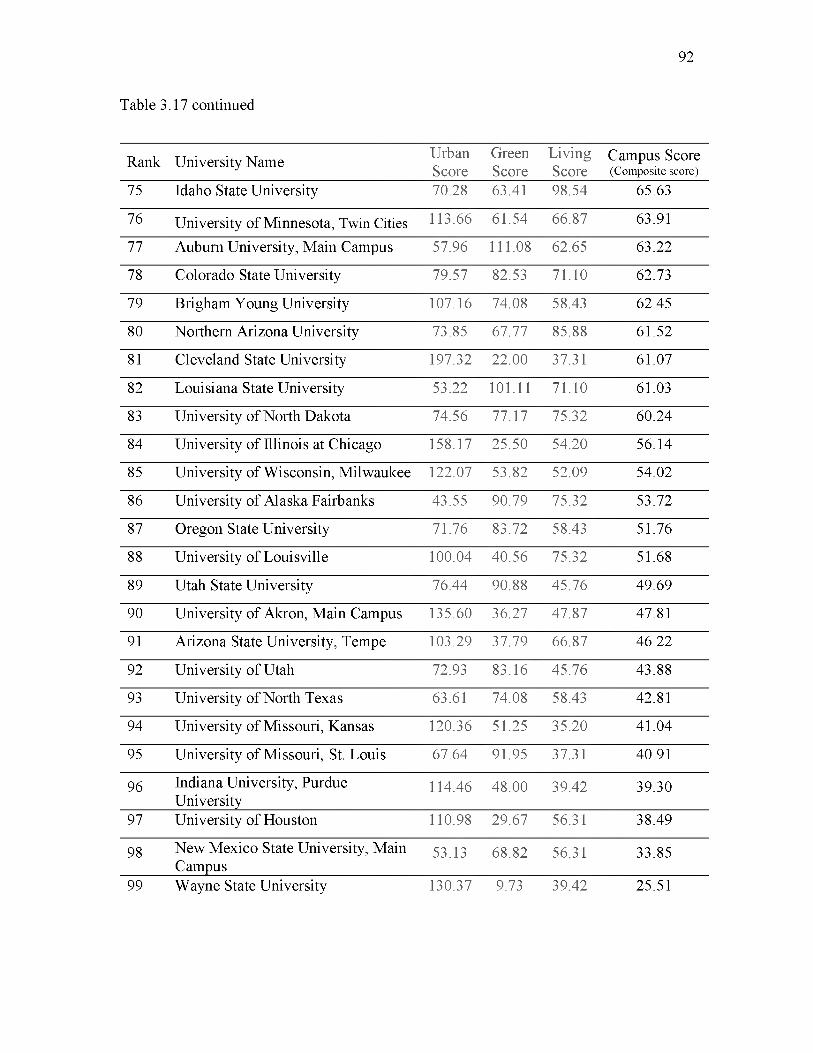
92
Table 3.17 continued
Rank University Name UrbanScore
GreenScore
LivingScore
Campus Score(Composite score)
75 Idaho State University 70.28 63.41 98.54 65.63
76 University of Minnesota, Twin Cities 113.66 61.54 66.87 63.91
77 Auburn University, Main Campus 57.96 111.08 62.65 63.22
78 Colorado State University 79.57 82.53 71.10 62.73
79 Brigham Young University 107.16 74.08 58.43 62.45
80 Northern Arizona University 73.85 67.77 85.88 61.52
81 Cleveland State University 197.32 22.00 37.31 61.07
82 Louisiana State University 53.22 101.11 71.10 61.03
83 University o f North Dakota 74.56 77.17 75.32 60.24
84 University o f Illinois at Chicago 158.17 25.50 54.20 56.14
85 University o f Wisconsin, Milwaukee 122.07 53.82 52.09 54.02
86 University of Alaska Fairbanks 43.55 90.79 75.32 53.72
87 Oregon State University 71.76 83.72 58.43 51.76
88 University o f Louisville 100.04 40.56 75.32 51.68
89 Utah State University 76.44 90.88 45.76 49.69
90 University o f Akron, Main Campus 135.60 36.27 47.87 47.81
91 Arizona State University, Tempe 103.29 37.79 66.87 46.22
92 University o f Utah 72.93 83.16 45.76 43.88
93 University o f North Texas 63.61 74.08 58.43 42.81
94 University of Missouri, Kansas 120.36 51.25 35.20 41.04
95 University of Missouri, St. Louis 67.64 91.95 37.31 40.91
96 Indiana University, Purdue University
114.46 48.00 39.42 39.30
97 University of Houston 110.98 29.67 56.31 38.49
98 New Mexico State University, Main Campus
53.13 68.82 56.31 33.85
99 Wayne State University 130.37 9.73 39.42 25.51

93
Table 3.17 continued
Rank University Name UrbanScore
GreenScore
LivingScore
Campus Score(Composite score)
100 University of Texas at San Antonio 32.94 101.29 28.87 24.98
101 University of Texas at Arlington 78.95 41.56 41.53 21.11
102 University of Colorado Denver 118.89 22.05 28.87 20.33
103 University of Nevada, Las Vegas 121.34 17.87 28.87 19.15

94
Table 3.18 The regression weights (ML and Bayesian) in modeling campus crime17
Maximum Likelihood Bayesian
Reg.Weights
St. Reg. Weights
Pvalue
Reg.Weights
95%Lowerbound
95%Upperbound
GRN1 <-- Green 1.000 .796 1.000GRN2 <-- Green 1.168 .661 *** 1.116 0.748 1.578GRN3 <-- Green -.300 -.575 *** -0.282 -0.441 -0.149CON1 <-- Urban 1.000 .665 1.000CON2 <-- Urban .853 .245 .012 0.856 0.130 1.584URB1 <-- Urban 33.160 .854 *** 33.695 25.58 45.11URB2 <-- Urban .113 .306 .004 0.115 0.038 0.201URB3 <-- Urban 149.479 .785 *** 151.877 112.5 205.4DEN1 <-- Urban 19.881 .825 *** 20.187 15.18 27.13GRN3 <-- Urban -10.144 -.696 *** -10.031 -15.23 -6.050GRN2 <-- Urban -16.148 -.327 .001 -17.110 -28.04 -6.460INHB <-- Living 1.000 1.000 1.000
CrimeRate <-- SAT -.009 -.290 .033 -0.009 -0.018 0.000CrimeRate <-- Profile -.105 -.341 .011 -0.106 -0.193 -0.020CrimeRate <-- Faculty .086 .286 .015 0.086 0.012 0.160CrimeRate <-- Urban -5.671 -.487 .002 -5.740 -10.25 -2.032CrimeRate <-- Green -.089 -.214 .164 -0.084 -0.228 0.042CrimeRate <-- Living .063 .371 .005 0.062 0.017 0.110CrimeRate <-- Climate -.001 -.216 .018 -0.001 -0.001 0.000CrimeRate <-- Income .053 .211 .017 0.054 0.012 0.124
17 Dropping the covariates/control variables changes the coefficients, but does not change their signs and the significance levels of campus form variables. The coefficient estimates would be: Urban: -2.912; Green: -.081; Living: 0.90

95
Table 3.19 The regression weights (ML and Bayesian) in modeling students’ commutingbehavior18
Maximum Likelihood Bayesian
Reg.Weights
Std.Reg.
Weights
Pvalue
Reg.Weights
95%Lowerbound
95%Upperbound
Walk Student<--Urban 3.477 .057 .737 4.493 -21.54 32.701Walk Student<--Green .309 .140 .467 .336 -.695 1.478Walk Student<--Living .367 .416 .008 .364 .046 .672Walk Student<--Locale .224 .007 .951 .263 -9.402 10.040Walk Student<--Profile -4.738 -.151 .278 -4.742 -14.06 4.661Walk Student<--Research -8.550 -.205 .071 -8.524 -19.39 2.407Car Student<--Urban -24.068 -.382 .022 -27.560 -58.73 -2.828Car Student<--Green -1.055 -.460 .012 -1.113 -2.346 -.129Car Student<--Living -.294 -.321 .025 -.288 -.578 .025Car Student<--Locale -6.951 -.221 .042 -6.956 -16.19 2.154Car Student<--Profile 7.970 .245 .053 7.953 -.912 16.757Car Student<--Research 12.499 .289 .005 12.567 2.168 22.892Transit Student<--Urban 27.702 .571 .003 30.985 9.699 58.426Transit Student<--Green .883 .500 .015 .921 .082 1.953Transit Student <--Living -.055 -.078 .628 -.059 -.326 0.192Transit Student <--Locale 6.836 .281 .021 6.802 -1.095 14.876Transit Student <--Profile -3.646 -.145 .305 -3.608 -11.20 4.049Transit_Student<--Research -4.787 -.143 .215 -4.879 -13.85 4.157
18 Dropping the covariates/control variables changes the coefficients, but does not change their signs and the significance levels of campus form variables, except for two. The coefficient estimates of “percentage of students living on campus” on “percentage of students who drive alone”, and “the degree of greenness” on “percentage of students who use transit” are not significant after dropping the covariates. The coefficient estimates would be: Urban -> Walk_Student: 1.599; Green-> Walk_Student: .333; Living -> Walk_Student: .342; Urban -> Car_Student: -24.380; Green-> Car_Student: -1.035; Living -> Car_Student: -1.93; Urban -> Transit_Student: 24.018; Green-> Transit_Student: .670; Living -> Transit_Student: -.056.

96
Table 3.20 The regression weights (ML and Bayesian) in modeling employees’ commuting behavior19
Maximum Likelihood Bayesian
Reg.Weight
Std.Reg.
Weight
Pvalue
Reg.Weight
95%Lowerbound
95%Upperbound
Walk Employee <--Urban -.179 -.007 .967 0.021 -11.16 11.306Walk Employee <--Green -.225 -.276 .176 -0.210 -0.653 0.249Walk Employee <--Living .077 .217 .215 0.074 -0.068 0.216Walk Employee <--Locale -.824 -.067 .615 -0.758 -5.275 3.778Walk Employee <--Profile -3.429 -.271 .083 -3.447 -7.838 0.907Walk_Employee<-Research -4.600 -.273 .032 -4.590 -9.505 0.346Car Employee <--Urban -34.545 -.609 .000 -38.400 -66.10 -16.11Car Employee <--Green -.358 -.185 .284 -0.401 -1.355 0.428Car Employee <--Living -.126 -.149 .312 -0.120 -0.400 0.168Car Employee <--Locale -1.824 -.063 .580 -1.839 -10.50 6.893Car Employee <--Profile 7.011 .234 .078 6.811 -1.936 15.624Car_ Employee <--Research 13.295 .333 .002 13.084 3.179 23.100Transit Employee <--Urban 40.684 .865 .000 44.977 27.423 69.174Transit Employee <--Green .688 .429 .008 0.721 0.120 1.458Transit Employee<--Living .050 .071 .587 0.047 -0.168 0.249Transit Employee<--Locale 1.715 .071 .470 1.643 -4.850 8.105Transit Employee<--Profile -1.867 -.075 .514 -1.618 -8.105 4.786Transit_Employe<-Research -5.142 -.155 .097 -4.919 -12.21 2.384
19 Dropping the covariates/control variables changes the coefficients, but does not change their signs and the significance levels of campus form variables. The coefficient estimates would be: Urban -> Walk_Employee: -1.972; Green-> Walk_Employee: -.207; Living -> Walk_Employee: .053; Urban -> Car_ Employee: -35.088; Green-> Car_ Employee: - 4.75; Living -> Car_ Employee: -.059; Urban -> Transit_ Employee: 40.326; Green-> Transit_ Employee: .670; Living -> Transit_ Employee: .043.

97
Figure 3.1 Connectivity map. The Integration R3 measure of street network of NewHaven County

98
Figure 3.2 Configuration map. The spatial configuration of Yale University

99
Figure 3.3 Modeling Campus Form. Left: the interaction of all dimensions, Right: all dimensions without land use organization and configuration. The remaining latent variables are: Urban= the degree of urbanization, Green= the degree of greenness, and Living= the degree of campus living
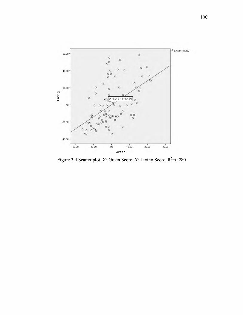
Livi
ng
100
Green
Figure 3.4 Scatter plot. X: Green Score, Y: Living Score. R2=0.280

Urb
an
101
Green
Figure 3.5 Scatter plot. X: Green Score, Y: Urban Score. R2=0.377

Urb
an
102
Living
3.061 E-4
Figure 3.6 Scatter plot. X: Living Score, Y: Urban Score. R2=0

103
Figure 3.7 Modeling students’ satisfaction and learning outcome. FRR: freshman retention rate; GRA6: percentage of students graduating in 6 years; UnderGrad: the total number of undergraduate enrollment (1 equals 1000 students); SAT: average SAT score; Faculty: percentage of classes with fewer than 20 students; Research: Type of university (Research I or Research II)

Mean
of
Cam
pus
Scor
e
104
Northeast Northeast M idwest Midwest West West South SouthResearch I Research 11 Research 1 Research II Research 1 Research II Research I Research II
Figure 3.8 Means of Campus Score for each census region and university type.

FRR
105
CScore
Figure 3.9 Scatter plot. X: Campus Score, Y: Freshman Retention Rate. R2=0.530
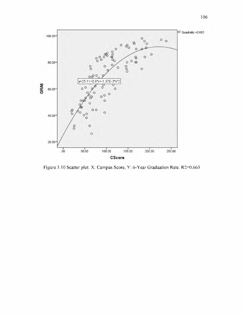
106
Figure 3.10 Scatter plot. X: Campus Score, Y: 6-Year Graduation Rate. R2=0.663

107
Figure 3.11 Modeling campus crime rate. Profile: the percentage of undergrad students, SAT: Average of SAT score, Faculty: the percentage of classes with fewer than 20 students, Income: the median household income of city; Climate: sum of cooling and heating days index

108
o.
Figure 3.12 Modeling students’ commuting behavior. Locale: the degree of urbanism of location, Profile: Enrollment profile classification, Research: Research I or Research II
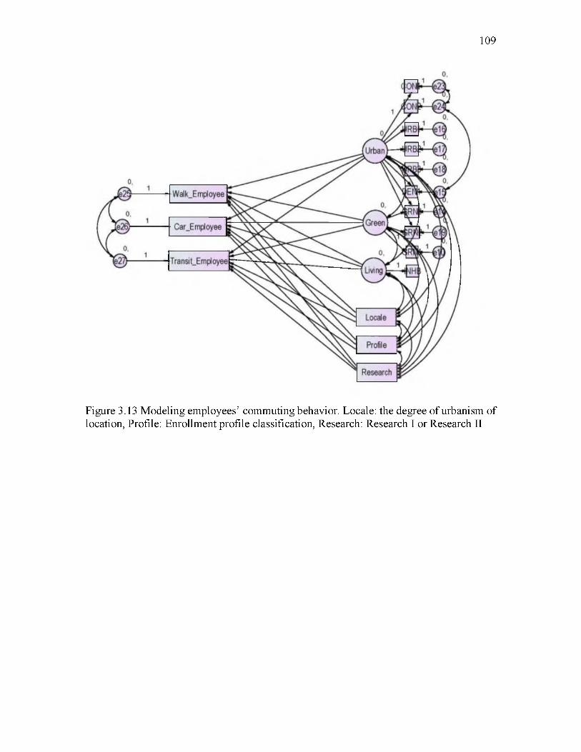
109
Figure 3.13 Modeling employees’ commuting behavior. Locale: the degree of urbanism of location, Profile: Enrollment profile classification, Research: Research I or Research II

CHAPTER 4
SUMMARY AND PERSPECTIVES
The United States of America has a rich history of campus planning and design.
Some of the best university campuses in U.S. were almost fully developed in the 19th
century and early 20th century. Before World War II, campus designers would follow
certain formal typologies such as quadrangle campus (e.g., University of Washington in
Seattle), picturesque campus (e.g., University of Vermont), or Beaux-Arts campus (e.g.,
Columbia University). After World War II, with the vast expansion of university campuses,
the emphasis was more on the design o f freestanding buildings than on campus master
plans. In recent years, most universities re-embraced the idea of campus master plans to
address their institutional objectives, such as attracting more prospective students,
increasing the quality o f life o f current students and faculty, promoting a learning and
research environment, creating a sustainable environment, and benefiting the surrounding
communities.
It became clear from the literature review that although campus planning and design
have received extensive attention in the profession in recent years, this field is understudied
in academia. In this research, I distilled a normative theory about the morphological
dimensions of the “Well-Designed Campus” through the content analysis of 50 randomly
selected campus plans, and also evaluated this theory quantitatively, using structural
equation modeling. In other words, I conceptualized the “well-designed” campus—in the

111
hypothesis-generating phase—to answer my first research question: What are the principal
features o f contemporary university campus planning and design? I then evaluated the
“well-designed” campus—in the hypothesis-testing phase—to answer my second research
question: And when implemented, are they correlated with university objectives such as
student success and satisfaction, campus safety and sustainability?
In this section, I summarize and discuss the main findings of both phases. In
addition, I briefly describe the limitations of study and the future research projects that can
be initiated based on the theoretical framework of this dissertation.
4.1 The Main Findings of the Hypothesis-Generating Phase
My first observation was the high degree of similarities between the challenges,
objectives, and recommendations of the reviewed master plans, which was surprising.
These similarities point to certain threats and opportunities for campus planning and design
practice. First, it may suggest that most campus planners have reached a shared, though
unstated, normative theory in their practice. I have distilled four big ideas from the most
common recommendations: 1) transition from a commuter campus to a convenient campus;
2) from an isolated campus to a contextual campus; 3) from a segregated campus to a
cohesive campus; and 4) from a brown campus to a green campus. However, due to the
scope of these similarities, the biggest challenge facing campus planners is the
predictability of the master plans. Campuses may lose their distinct character and identity
if they only adopt generic recommendations. The most successful campuses would be those
that keep the element of uniqueness and sense of place in their master plans, while
simultaneously following the common norms of practice.

Another key lesson from the content analysis of master plans is the high chance of
infill development over campus expansion, at least in the near future. While almost all
campus plans pointed out the deficits in square footage as their top challenge, only four
percent o f campus plans mentioned the deficits in land for potential growth in their
documents. In addition, it was unexpected that promoting walkability was a shared
objective in all reviewed master plans, while promoting a learning environment was
mentioned in less than half of the plans. This finding indicates that campus planners may
not fully treat the physical campus as an asset to enhance learning, or there are fewer known
physical interventions at the campus level that can address this objective.
In order to avoid a subjective definition o f what constitutes a “well-designed”
campus, I referred to the most common recommendation in the selected master plans.
Therefore, one o f the biggest contributions to this dissertation research is providing a
theoretical framework to study campus form through the lens o f practitioners. To evaluate
campus form, seven dimensions are suggested: land use organization, compactness,
connectivity, configuration, campus living, greenness, and context. These dimensions are
measurable; therefore, it was possible to test their relationship to the desired outcomes
quantitatively.
4.2 The Main Findings o f the Hypothesis-Testing Phase
Exploring the relationships between campus form and the desired outcomes, such
as students’ satisfaction, safety, and campus sustainability, gives campus planners fresh
insight into the possible consequences of their actions. In addition, quantifying dimensions
o f campus form can inform campus planners about the norms o f campus design for
different university types in different census regions. For example, the percentage of
112

surface parking areas or the percentage of pervious surfaces of one campus can be
compared to the mean value of these variables for similar institutions. Furthermore,
mapping 103 campuses in ArcGIS (half of the total research universities in the U.S.), a
main step in the quantifying process, can be a valuable source of information for those who
want to study campus plans at the national level.
Three dimensions are highly correlated to each other: compactness, connectivity,
and context. I could generate more stable models by creating a new latent variable from
these three dimensions. This latent variable is measuring “the degree of urbanism” of a
campus. In other words, campuses that are more compact, better connected internally and
to their surroundings, and are located in a more urban context, have a higher degree of
urbanism. I found this latent variable, along with “the degree of greenness” and “campus
living,” to have significant association with more than one of the outcome variables. The
tested models did not show any significant association between two campus form
dimensions— configuration and land use organization— and the outcome variables. These
two dimensions were the only dimensions that I had to rate subjectively. Therefore,
although I tested for the reliability of these measurements, the possibility of a substantial
measurement error as a contributing factor for the observed results is likely. However, the
fact that these factors have truly no significant association with the outcome variables is
also very much possible.
One of the interesting findings of this research is that although greenness and
urbanism are negatively correlated to each other, both are positively associated with
students’ satisfaction with their college experience, controlling for the other university
qualities. This finding can shed light on a classic debate among campus planners and
113

designers about the dichotomy of a green and pastoral campus versus an urban campus.
The results show that campuses must have a fair amount of both qualities to get a high
design score. It is important to note that greenness is measured in a quarter mile buffer
around campus buildings and not just on the campus ground, since accessibility is more
important than ownership. Therefore, universities that are located in an urban setting
should be sensitive not just about the greenness of their campus, but also the accessibility
to local parks and green spaces. Likewise, universities with rural and suburban campuses
should plan for and support more activities in their adjacent urban areas.
Another major finding is the strong association of on campus living with student
satisfaction and graduation rate, after controlling for other influential factors. As described
in the result section, a 10% increase in on campus residents is associated with the increase
of the 6-year graduation rate of 2.43%. This finding suggests that campus housing may not
just provide a convenient residence for students, but it can also largely impact the quality
of life and education. Most importantly, improvement in this aspect of campus form is
more feasible and economical than greenness or urbanism. I should note that while the
number of students living on campus is important, their quality of living is even more so.
I did not measure the quality of students’ living in university housing of the selected
campuses, but in the reviewed master plans, certain qualities were highlighted. For
example, student housing should be close enough to the campus core to make it convenient
for students to walk or bike to major destinations on campus. Students should also have
reasonable housing choices in respect to housing type, style, and cost. In addition,
universities should pursue innovative housing typologies. For example, the University of
Utah launched an ambitious plan to recruit the “400 best student entrepreneurs” to live in
114

a $45 million residential building starting Fall 2016. The goal is to create a place where
student entrepreneurs “live, create, launch.”20
Based on the qualities of urbanism, greenness, and campus living, I ranked my
sample population (103 campuses). I developed a composite score— Campus Score—from
the following formula: 0.177 X Urban+0.215 XGreen+0.251 X Living. The three latent
variables were standardized with the mean of 0 and standard deviation of 1. The multipliers
are adopted from the standardized regression weights of the freshman retention rate model.
Columbia University, Princeton University, Lehigh University, Duke University, and
Emory University had the highest Campus Scores and University of Nevada at Las Vegas,
University of Colorado at Denver, University of Texas at Arlington, University of Texas
at San Antonio, and Wayne State University had the lowest Campus Scores.
The ANOVA test for the Campus Score of each census region and university type
reveals that there is a significant difference between different categories. Private
universities have significantly higher mean scores than public schools, Research I
universities have significantly higher mean scores than Research II universities, and
universities in the Northeast census region have significantly higher mean scores than
universities in other census regions. This finding may raise certain questions, such as
whether campus form has any true influence on freshman retention rate and 6-year
graduation rate, or is it simply that better institutions have better campuses, and physical
campus has no true influence on students’ overall satisfaction and graduation rate.
115
20 For more information about this project go to http://lassonde.utah.edu/u-of-utah- recruiting-the-400-best-student-entrepreneurs/
To answer this question I controlled for all the main control variables in the
literature for measuring university qualities, such as average SAT score as a proxy for
student selectivity, the percentage of classes with fewer than 20 students as a proxy for
faculty resources, a dummy variable for Research I or Research II universities as a proxy
for research capacity, and finally the total number o f undergraduate students as a proxy for
the size o f the institution. After controlling for these factors, campus form factors still have
significant association with freshman retention rate and 6-year graduation rate. There might
be a simple explanation for these relationships. Although it is hard to imagine that one
student decides not to continue his or her education solely due to the campus qualities, it is
much more likely that a green, urban, and livable campus provides such an enriching
experience that students are convinced to pursue their education against all the potential
negative factors, such as financial or academic issues.
The fact that the universities in the northeast region have higher Campus Scores is
not just because of the eminence of their institutions in general; it can also be due to the
type o f urbanism in that region and, most importantly, the age o f the campuses. Most
campuses in that region were almost fully developed before the mid-20th century when
campus planning was following certain established formal typologies rather than being
dominated by auto-oriented development patterns and star architects. In addition, not all
universities in the northeast region have high Campus Score. For example, Rutgers campus
ranking is 71. Also, from the top 20 campuses, seven of them are not in the northeast:
Emory University (rank 5), Stanford University (rank 7), College of William & Mary (rank
9), Case Western Reserve University (rank 11), Washington University in St. Louis (rank
16), University of Notre Dame (rank 17), and Rice University (rank 19).
116

The most interesting lesson from studying the relationship of campus safety and
campus form was that more urbanized campuses are actually associated with less crime on
campus, not more crime. This finding can be explained by the concept of “eyes on the
street” coined by Jane Jacobs in her classic book, The Death and Life o f Great American
Cities. More activities surrounding a campus mean more potential witnesses or interveners,
which can enhance the level of safety. On the other hand, one of the challenges with a
higher percentage of students living on campus is potentially more crime on campus. This
may seem to counter the “eyes on the street” argument, but it can be justified by the fact
that it is more difficult to provide security for a large population than a small one. The
important and logical lesson for university administrators is the necessity of providing
adequate security services if a large percentage of students live on campus.
One of the benefits of a higher percentage of students living on campus, however,
is the opportunity for more sustainable modes of transit, such as a higher percentage of
students who walk or bike to class and a lower percentage of students who commute with
only the driver in the vehicle.
The degree of campus greenness and urbanism are also both associated with more
sustainable modes of travel. There are explanations to justify these associations. First,
turning surface parking areas into green spaces or new buildings can increase the degree of
campus greenness, and also make finding parking spaces harder and probably more costly
for students and employees; therefore, they may find alternative modes of transportation to
be more convenient.21 In addition, there are more housing opportunities surrounding an
117
21 This is a concept similar to the “reduced demand” phenomenon (the opposite of “induced demand”) in transportation: decreasing road capacity increases the cost of travel so demand is reduced (Cervero and Hansen, 2002).
urban campus, and probably more transit opportunities; therefore, a lower percentage of
students and employees may choose to commute by their own vehicles. Finally, a greener
campus can provide a more pleasant walking and biking experience, and therefore, can
increase the probability of walking and biking. For example, a 15-minute walk across
parking lots and unplanted sidewalks can be undesirable, while a 15-minute walk across a
green campus can become a pleasant daily ritual.
Overall, I theorized the “Well-Designed Campus” as a campus that is mixed,
dense, well-connected, well-structured, inhabited, green, with an urbanized setting. The
hypothesis was that the “Well-Design Campus” supports sustainable, livable learning
environment. From the Structural Equation Models, I concluded that certain
morphological aspects of “Well-Designed Campus” are significantly associated with the
selected university objectives. It is important to understand that I evaluated a common
big concept in the practice of campus design, not any specific recommendation. For
example, this research does not specifically assess the validity of a recommendation such
as “encouraging mixed-use development along a street corridor at the campus border”;
however, this recommendation may increase the degree of urbanism of campus, which is
proved to be a positive quality. Although, I extracted 100 recommendations from the
reviewed campus plans, clearly they don’t have the same power and impact on campus
quality. If I want to further translate my findings into lessons for practitioners, I should
stress those recommendations that are most crucial for creating a “Well-Designed
Campus.” The first and foremost recommendation would be to increase on campus
housing. The second recommendation would be to decrease surface parking areas. And
the third recommendation depends on the campus setting. For the urban campuses, the
118

third recommendation would be to invest in green spaces on and adjacent to campus. For
suburban and rural campuses, the third recommendation would be to encourage infill and
mixed-use development on and adjacent to campus.
4.3 Limitations of Study
The biggest limitation of this research is data availability. Although data on
institutional characteristics are diverse and relatively accessible, very little information on
the built environment characteristics of university campuses is available. Information such
as building height and architectural quality of campus buildings is not available and
therefore, not included in this research. The lack of data availability is the main limitation
for operationalizing morphological constructs, such as land use organization and
configuration.
Although this study provides a theoretical framework for analyzing normative
dimensions of campus form, testing the validity of these dimensions requires more research
on measuring outcome variables, such as livability, sustainability and learning outcomes.
For this dissertation, I have had to rely on the available proxy variables. For example, the
validity of STARS can be a problem because this index has been produced through a self
report survey by universities without any inspection or validation by AASHE. Measuring
control variables is also challenging. For example, a key control factor— administrative
policy—is missing in this study. The administrative policy of universities can have a
critical impact on achieving different institutional objectives. Proxies such as “type of
institution” or “enrollment profile” cannot fully represent the complexity of administrative
policies in addressing institutional missions. The final limitation relates to the unit of
119

120
analysis o f this research. Because o f data availability, I have to use the campus as the unit
o f analysis, which is a highly aggregated unit.
4.4 Future Research
As Brenda Scheer (2010) described:
It is easy to see that a campus is a very different construct than a piece o f a city. It mimics only the look, not any o f the other urban qualities or conditions that provide the resilience of naturally evolved places and types. Those qualities include regular and divided lot patterns, public streets, relatively simple building types situated individually on lots, and multiple connections to surrounding fabrics (p. 46).
Overall, a campus is not a city, a neighborhood, or a block. Therefore, describing and
analyzing the morphology o f a campus should be different from other aspects o f the built
environment. This study, for the first time, has proposed seven morphological dimensions
for analyzing campus form. The proposed theoretical framework can be related to different
research topics in regards to university campuses.
Based on the proposed morphological dimensions, it is possible to propose the
typology o f university campuses. Understanding the typology o f university campuses can
inform campus planners and university administrators about the potential challenges and
opportunities that are associated with their specific campus type. In addition, proposing a
campus typology is a key step in investigating the potential relationship between different
campus types and the institutional identity o f universities. Finally, the typology o f
university campuses can shed light on the dynamics of town-gown relationships.
Research on the impact of university interventions on surrounding neighborhoods
is limited. There are some detailed case studies on campus expansion and neighborhood
revitalization in the past decades; some of them were successful projects, some of them
were not. However, we don’t really know if the morphology of the campus and
neighborhood and their physical interaction are the influential factors for the success of
university interventions. To conduct systematic research in this area, the proposed
theoretical framework for analyzing campus form is critical.
Other possibilities for related future research include exploring the relationships
between campus scare and various university rankings such as U.S. news and world report,
Times Higher Education, and Shanghai rankings; applying the same basic methodology to
nonresearch institutions such as community colleges and regional universities; applying
the technique of propensity score matching to see if it is campus design or “the northeast
effect” that causes schools such as the Ivy Leagues to score so high in terms of outcomes.
121

APPENDIX A
THE TOP 100 CAMPUS MASTER PLAN RECOMMENDATIONS

123
Recommendations for transforming university campuses, sorted by their theme, objective,
and frequency: * =1-9 cases, **=10-19 cases, ***=20-29 cases, ****=30-39 cases,
*****=40-50 cases.
CONVENIENT CAMPUS
LIVABILITY
1
2
4
5
7
8
10
11
12
13
**
Increase residential housing on campus.
Locate as many university functions as possible on or close to Central Campus (without compromising the highly valued sense of openness in some cases).
Increase recreational and cultural amenities like fitness-exercise facilities, performing arts center, and visual arts facilities.
Increase and Improve gathering spaces (with quality furniture).
Enhance the quality of the campus environment by including quality public art that reflects the spirit and creativity of University.
Encourage mixed-use development and buildings with active ground- level uses.
Broaden and diversifying housing options on campus.
Dining services will be distributed throughout the campus. Introduce smaller food venues within the academic core.
Install lighting in parking lots and garages, for comfort and security, but with minimal glare to the immediate surroundings.
Reasonable accommodations for students with physical disabilities; Installing ADA compliant ramps • Making curb cuts in sidewalks and entrances • Widening doors • Installing offset hinges to widen doorways • Installing accessible door hardware.
Designated zones on campus, selected on the basis of location, proximity of resources and amenities, and safety, will host a range of academic and social activities during extended hours to encourage activities 24/7.
SENSE OF COMMUNITY
Create an academic neighborhood hub by providing a central space for student-focused and student-led activities.
Integrate academic and research activities in shared facilities.
3
6
9

124
14
15
16
17
18
19
20
21
22
23
24
25
26
27
28
29
30
**
**
**
Instead of creating pure residential districts, mix them with multidisciplinary academic facilities and have them on the core campus.
Recognize and support distinct communities of disciplines within the context of the larger University.
Emphasize close relationships and short travel times between related programs to encourage cross-disciplinary collaboration.
Creating a more transparent addition along the pedestrian path - so that building users and passersby can “see and be seen.”
Creates a system of internal circulation corridors with learning/social spaces.
Consolidate undergraduate academic divisions, as well as the facilities of individual professional schools as much as possible, to increase efficiency and maximize convenience for both faculty and students.
Intensify the overlap and magnitude of campus, workplace, residential, and amenity activities to foster creative innovation with a mix of people engaged in living, working, learning, and relaxing.
Protect and enhance outdoor teaching and research facilities.
WALKABILITY
Limiting expansion and using infill development where possible.
Changing some surface parking areas (mainly at the core of campus) into parking structures or other utilities.
Promote the use of alternative modes of transportation including shuttle and bicycles to reduce vehicular traffic.
Creating car-free zone -reducing vehicular through-traffic on campus.
Locate new parking to intercept traffic at the campus edge to reduce internal traffic and the need for shuttles.
Incorporate comprehensive bike network. Provide dedicated bike lanes, in both directions, on campus streets that are contiguous and easily understood by cyclists.
Plan and advocate for potential future regional passenger rail service and locate a future station to support campus circulation patterns.
Selectively redistribute parking capacity to be closer to high demand areas in and around the campus core and projected development areas.
Concentrate development around transit nodes.
*
*
*
*
*
*
*

125
31
32
33
34
35
36
37
38
39
40
41
42
43
Improving parking area efficiencies, maintenance and appearance through consolidation and screening.
Price parking to ensure financial sustainability and to encourage alternative mode use.
Reposition select campus bus stops to better align with primary pedestrian circulation routes and major roadway intersections.
The introduction of a car-share program to the university. This could provide options for resident students without cars to make trips to the grocery store or to frequent off-campus retail destinations.
Support efforts to make streets narrower to slow traffic and minimize the crosswalk distance.
Consolidate and reorganize service access routes to reduce potential pedestrian/vehicle conflicts.
Make the most efficient use of parking supply by locating facilities in places that support complementary uses during evenings and weekends. Also develop a hierarchy of parking as it applies to hourly commuters, daily commuters and residential customers.
Locate support structures, such as physical plant and grounds maintenance, at the perimeter of the campus, where they can meet functional and circulation needs more easily.
Align and simplify many existing pedestrian movements to ease navigation and to improve safety.
Increasing campus safety through separation of vehicles from many heavily-used pedestrian areas.
CONTEXTUAL CAMPUS
PARTNERING
Respond to community partnership opportunities, including: student convocation center, student dining, student union, theater, large banquet space, and alumni center.
An alliance with the City to create a mixed-use campus town along a street corridor which will provide both additional residential beds and needed retail services like restaurants, coffee shops, and potentially the university book.
Provides educational access opportunities throughout the region by establishing multiple locations.
*
*
*
*
*
*
*
*
*
*
44 * Provide community input where appropriate into the University Campus Master Plan process.
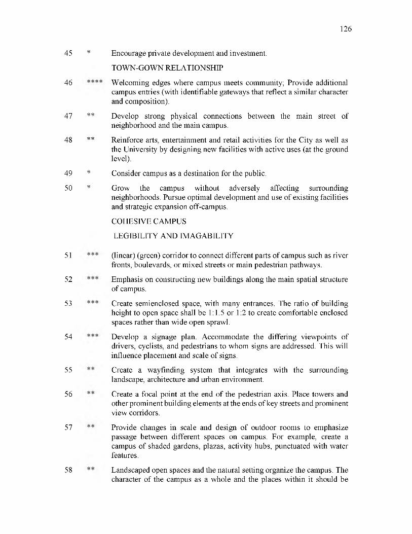
45
46
47
48
49
50
51
52
53
54
55
56
57
58
126
**
**
Encourage private development and investment.
TOWN-GOWN RELATIONSHIP
Welcoming edges where campus meets community; Provide additional campus entries (with identifiable gateways that reflect a similar character and composition).
Develop strong physical connections between the main street of neighborhood and the main campus.
Reinforce arts, entertainment and retail activities for the City as well as the University by designing new facilities with active uses (at the ground level).
Consider campus as a destination for the public.
Grow the campus without adversely affecting surrounding neighborhoods. Pursue optimal development and use of existing facilities and strategic expansion off-campus.
COHESIVE CAMPUS
LEGIBILITY AND IMAGABILITY
*
*
*
(linear) (green) corridor to connect different parts of campus such as river fronts, boulevards, or mixed streets or main pedestrian pathways.
Emphasis on constructing new buildings along the main spatial structure of campus.
Create semienclosed space, with many entrances. The ratio of building height to open space shall be 1:1.5 or 1:2 to create comfortable enclosed spaces rather than wide open sprawl.
Develop a signage plan. Accommodate the differing viewpoints of drivers, cyclists, and pedestrians to whom signs are addressed. This will influence placement and scale of signs.
Create a wayfinding system that integrates with the surrounding landscape, architecture and urban environment.
Create a focal point at the end of the pedestrian axis. Place towers and other prominent building elements at the ends of key streets and prominent view corridors.
Provide changes in scale and design of outdoor rooms to emphasize passage between different spaces on campus. For example, create a campus of shaded gardens, plazas, activity hubs, punctuated with water features.
Landscaped open spaces and the natural setting organize the campus. The character of the campus as a whole and the places within it should be
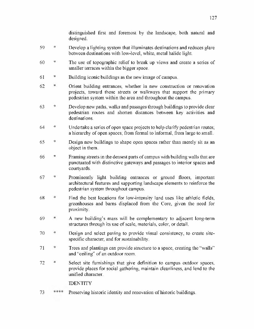
59
60
61
62
63
64
65
66
67
68
69
70
71
72
73
127
distinguished first and foremost by the landscape, both natural and designed.
Develop a lighting system that illuminates destinations and reduces glare between destinations with low-level, white, metal halide light.
The use o f topographic relief to break up views and create a series o f smaller terraces within the bigger space.
Building iconic buildings as the new image o f campus.
Orient building entrances, whether in new construction or renovation projects, toward those streets or walkways that support the primary pedestrian system within the area and throughout the campus.
Develop new paths, walks and passages through buildings to provide clear pedestrian routes and shorten distances between key activities and destinations.
Undertake a series o f open space projects to help clarify pedestrian routes; a hierarchy of open spaces; from formal to informal, from large to small.
Design new buildings to shape open spaces rather than merely sit as an object in them.
Framing streets in the densest parts o f campus with building walls that are punctuated with distinctive gateways and passages to interior spaces and courtyards.
Prominently light building entrances or ground floors, important architectural features and supporting landscape elements to reinforce the pedestrian system throughout campus.
Find the best locations for low-intensity land uses like athletic fields, greenhouses and barns displaced from the Core, given the need for proximity.
A new building’s mass will be complementary to adjacent long-term structures through its use of scale, materials, color, or detail.
Design and select paving to provide visual consistency, to create site- specific character, and for sustainability.
Trees and plantings can provide structure to a space, creating the “walls” and “ceiling” of an outdoor room.
Select site furnishings that give definition to campus outdoor spaces, provide places for social gathering, maintain cleanliness, and lend to the unified character.
IDENTITY
Preserving historic identity and renovation o f historic buildings.
*
*
*
*
*
*
*
*
*
*
*
*
*
*

128
74
75
76
77
78
79
80
81
82
83
84
85
86
87
88
89
**
**
**
**
Preserve and enhance views to and from character defining features.
Extend the formal pattern of quads, and courts as the character of campus.
Select materials that are consistent with campus standards.
Proposing design guidelines (based on typological studies of existing buildings and campus features such as benches, trash and recycling receptacles, tables, bicycle racks, fences, fighting, pavements, signage, emergency telephones).
Avoiding rectangular corporate looking buildings on campus.
Consider opportunities to demolishing old and small buildings and constructing more efficient buildings, in harmony with the campus character.
Develop at a higher density outside the core to preserve the historical character of core campus.
GREEN CAMPUS
ENVIRONMENTAL SUSTAINABILITY
Develop a green infrastructure from an ecological and aesthetic perspective, as well as engineering.
Site buildings and plant materials for microclimate characteristics such as cooling summer breezes, protection against winter winds, sunlight, and shade.
Promote on-site renewable energy from sources such as biomass and solar power to meet energy demand.
Orient (and pitch) roofs for solar thermal and photovoltaic applications (immediate or future).
Support long-term utilities planning and life cycle costing.
Technology is implemented in transportation including: clean fuels and vehicles; traffic operation systems that manage traffic flow and reduce delay and congestion on nearby roadways; advanced and accessible traveler information.
Easing campus maintenance through better unified and longer lasting amenities.
Plan campus growth on the most suitable sites possible, avoiding unnecessary environmental impacts to existing campus open space and natural resources.
Provide site lighting that is sensitive to light pollution of the night sky and minimizes impacts on nocturnal environments.
*
*
*
*
*
*
*
*
*

129
90
91
92
93
94
95
96
97
98
99
100
**
**
Reduce potable water consumption associated with landscape irrigation.
Create a campus-wide network of small scale storm water measures, such as constructing check-dams in forested swales; establishing rain gardens and bio retention; installing permeable pavements.
Use passive strategies such as insulation and shading to minimize energy demand.
Optimize buildings’ energy performance by using efficient mechanical and electrical systems.
LANDSCAPING
Addition of high-quality landscaping and site furnishings to create comfortable and lively open spaces.
Preserve park-like setting of campus.
Generously landscape setbacks and moats between buildings and city streets.
Breaking parking lots with (native) trees to create more manageable parking rooms and to perform ecological functions.
Be open to its natural features-a river or a hill-and remove obstacles to seamless integration. Integrate the planned and natural environments more fully with one another.
Integrate the native vegetation within future campus landscape development.
Setbacks and buffers from water bodies, streams, and wetlands to protect wildlife corridors, sensitive riparian zones, and water quality. Setbacks and buffers generally range from 25 feet to 100 feet.
*
*
*
*
*
*
*

APPENDIX B
ANALYTICAL MAPS FOR SELECTED CAMPUSES

131
, | T !/V W . / -/-/ / WWV'/V
i l l
♦
KM
l i
- n
• r w * 1tt ■
»# [ ^ 4
1̂ miijn ■ - 'j\ m~ i 1 Ii c : " " ci j o j a h m h. t i 1
-*-Sc: . -m' « i<
iE 3 f f i►
»_ —^ ~ —
N
A0 0.25 0.5 1
Figure B.1 Figure ground map, Oklahoma State University

132
Figure B.2 Pervious open space, Oklahoma State University22
In all “pervious open space” maps, black is impervious space.

133
Figure B.3 The intensity of tree canopy, Oklahoma State University
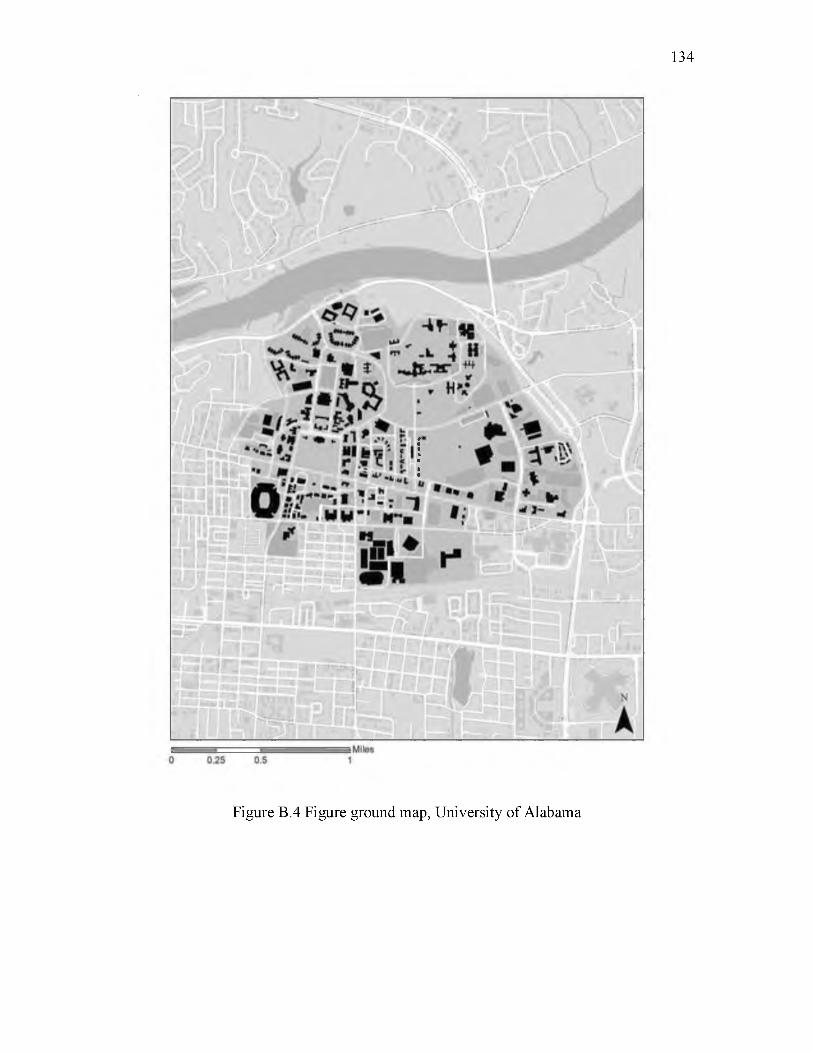
134
Figure B.4 Figure ground map, University of Alabama

135

136
Figure B.6 The intensity of tree canopy, University of Alabama

137
Figure B.7 Figure ground map, University of Albany, SUNY

138

139
Figure B.9 The intensity of tree canopy, University of Albany, SUNY

140
Figure B.10 Figure ground map, University of Massachusetts Amherst

141
Figure B.11 Pervious open space, University of Massachusetts Amherst

142
0 0.25 0.5 1
Figure B.12 The intensity of tree canopy, University of Massachusetts Amherst
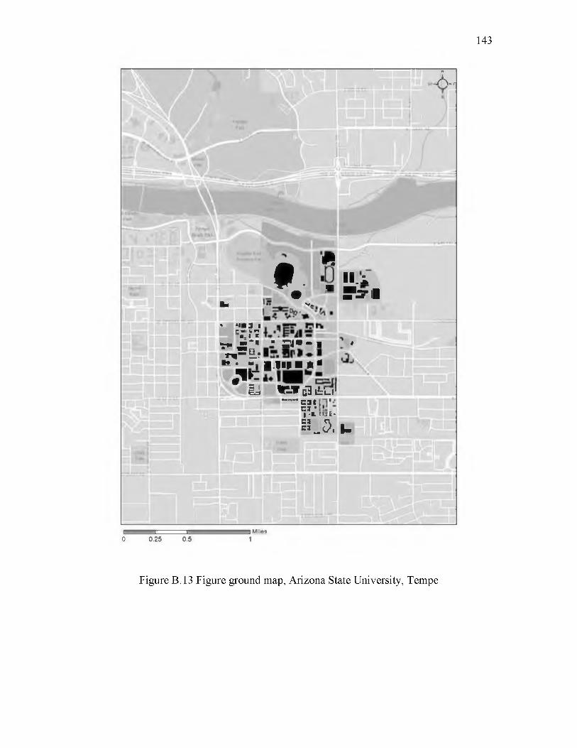
143
.A m
f . " H i
k
a■ • V.
f f j i
* MBS ■ r hi * **■_i c^ m ~ 9
V,= 3.r■ a « - i #
H • a.
3 kl.liia *■
WcllirU1
J* yEd
— cat« : E| -U. M3t*C3 a c * „ 0 , I.
Ctari j
' ' ■ - i M ila s0 0.25 0.5 1
Figure B.13 Figure ground map, Arizona State University, Tempe

144
Figure B.14 Pervious open space, Arizona State University, Tempe
145
Figure B.15 The intensity of tree canopy, Arizona State University, Tempe
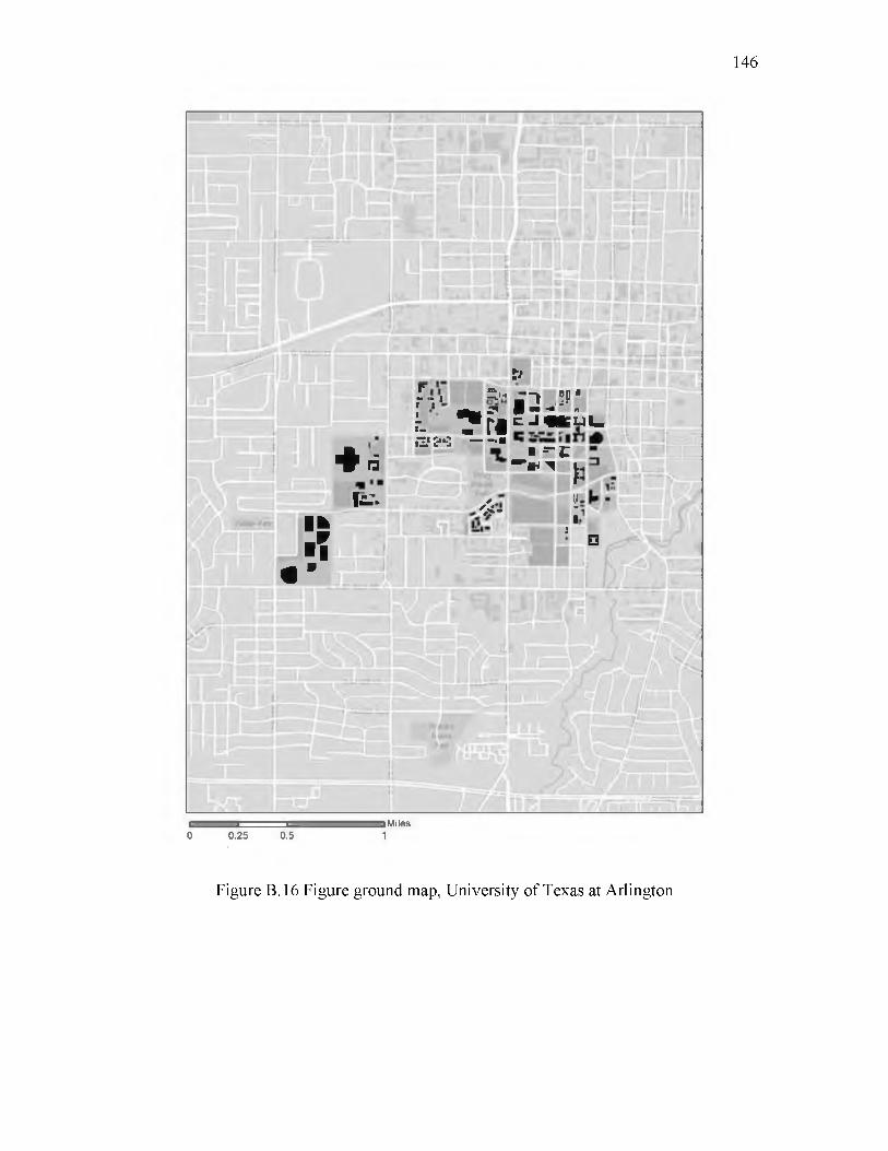
146
&rr■
- 1 1 ^
£>«i f . ■ 2 J ! :
c J fKLJl_
+ 6
la:.
r.ii1oo -C J n—■■
■ ="C
'U~
■"IK 1 | |
lj*■91
: ?
12 □m
*
1
5^5» < I —i Milns0 0.25 0.5 1
Figure B.16 Figure ground map, University of Texas at Arlington

147
Figure B.17 Pervious open space, University of Texas at Arlington

148
0 0.25 0.5 1
Figure B.18 The intensity of tree canopy, University of Texas at Arlington

149
Figure B.19 Figure ground map of Auburn University

150
Figure B.20 Pervious open space, Auburn University
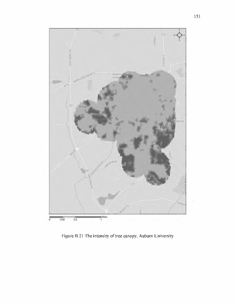
151
Figure B.21 The intensity of tree canopy, Auburn University

152
Figure B.22 Figure ground map, University of Colorado, Boulder
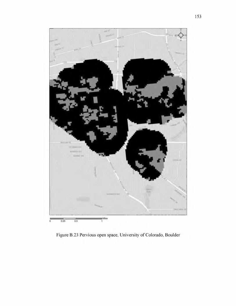
153

154
N
w-<VE
0 025 0.5 1
Figure B.24 The intensity of tree canopy, University of Colorado, Boulder

155
Figure B.25 Figure ground map, Binghamton University

156
Figure B.26 Pervious open space, Binghamton University

157
Figure B.27 The intensity of tree canopy, Binghamton University

158
Figure B.28 Figure ground map, Carnegie Melon University

159
Figure B.29 Pervious open space, Carnegie Melon University

160
Figure B.30 The intensity of tree canopy, Carnegie Melon University
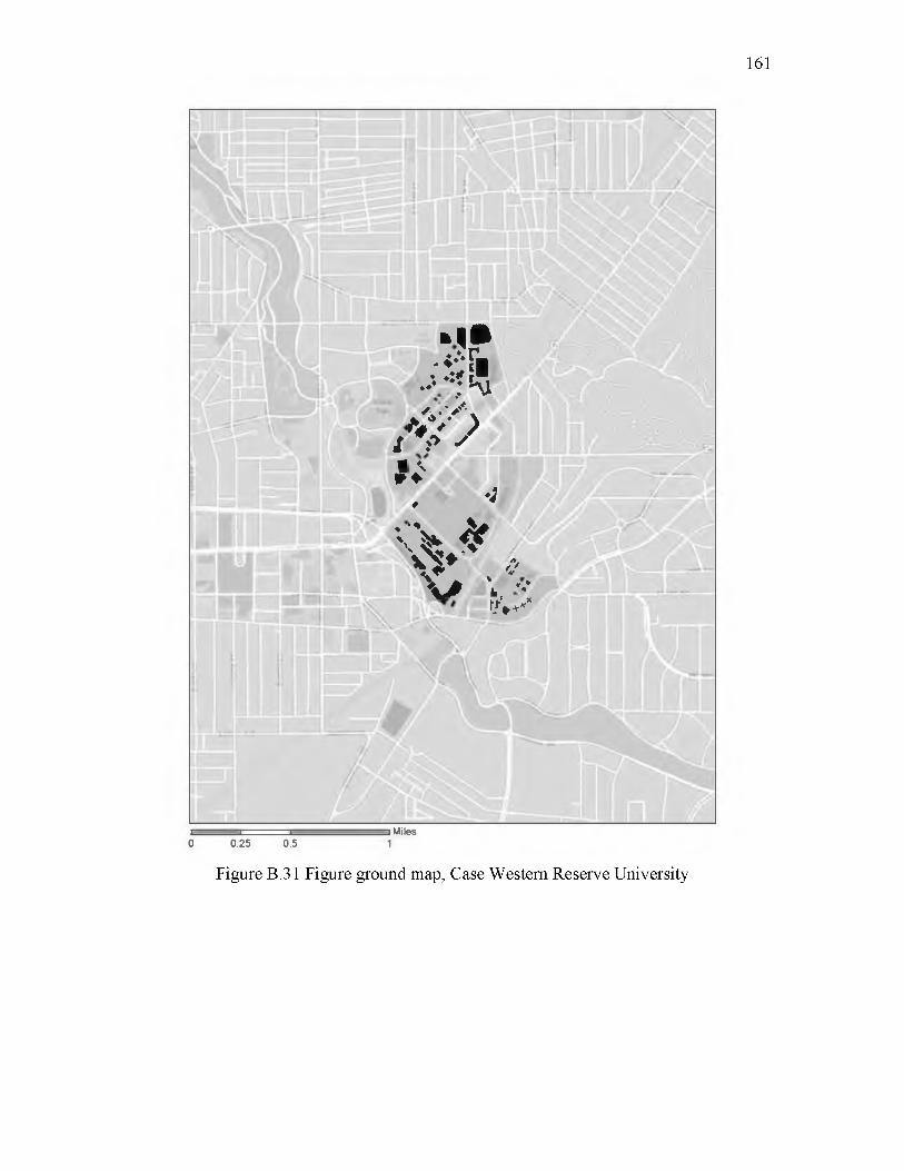
161
J
• L »: £ [ ■ ••• ; KiA.*/.
* V >s > y %
1 *, •;
♦\; v *v> . « Y > * •••
j-a 'i~
iln ?! ~s,̂ <vvr/V+*x
i i i ~i Mi l es0 0.25 0.5 1
Figure B.31 Figure ground map, Case Western Reserve University

162
i i i ~i Miles0 0.25 0.5 1
Figure B.32 Pervious open space, Case Western Reserve University
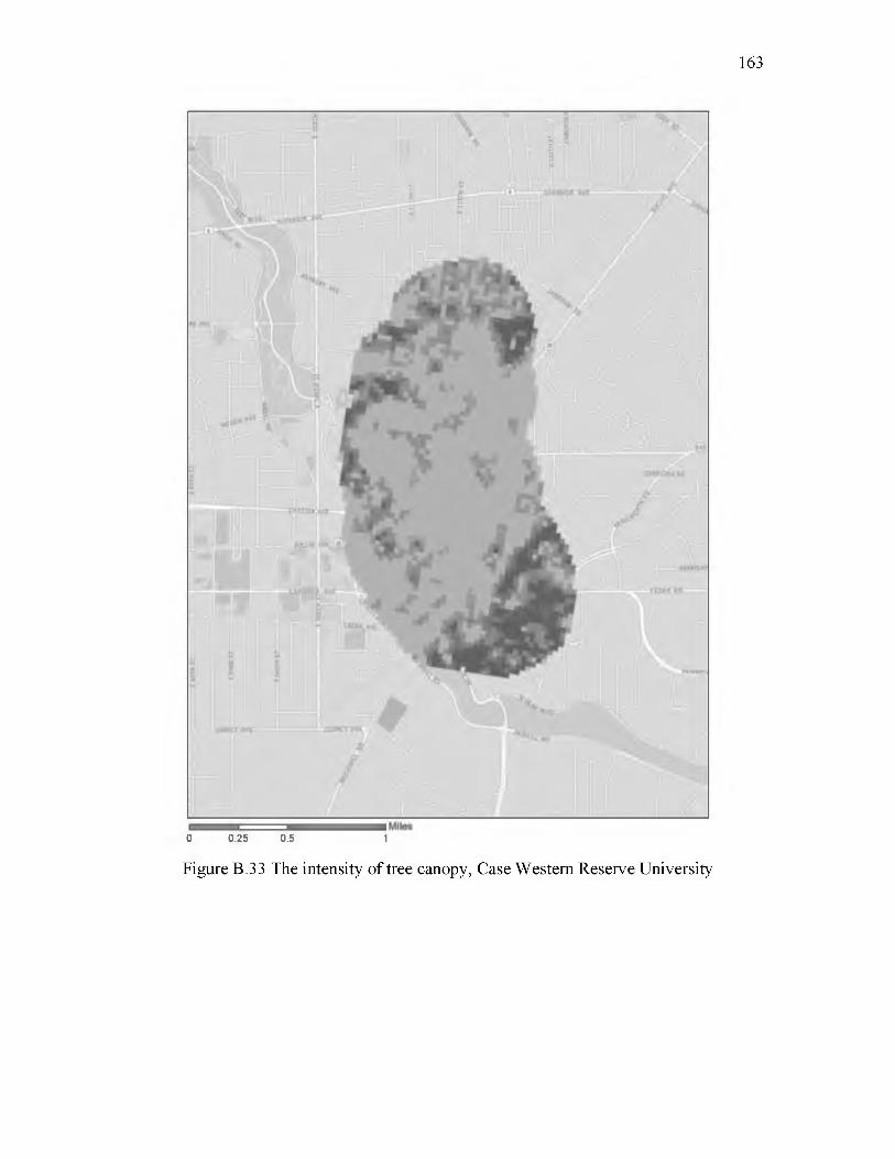
163
0 0.25 0.5 1
Figure B.33 The intensity of tree canopy, Case Western Reserve University

164
% \ * f ■>
' * * ♦&>i ISF*
' i i — i Mi l f i S
0 0.25 0.5 1
Figure B.34 Figure ground map, University of Colorado Denver

165
• 1118 M l
Figure B.35 Pervious open space, University of Colorado Denver

166
Figure B.36 The intensity of tree canopy, University of Colorado Denver

167
1■ “ ̂I-' ~! ■ J L~- ■ ).r
|W 8Pill-.' 1 l|l» l\m r&a■ - t jr r - i .L * £ -""JS . .. « | i ■■ H*»il • tl
■5 2.s 1
nnri iii":ill'll'! .m
Mi l es0 0.2S 0.5 1
Figure B.37 Figure ground map, Colorado State University
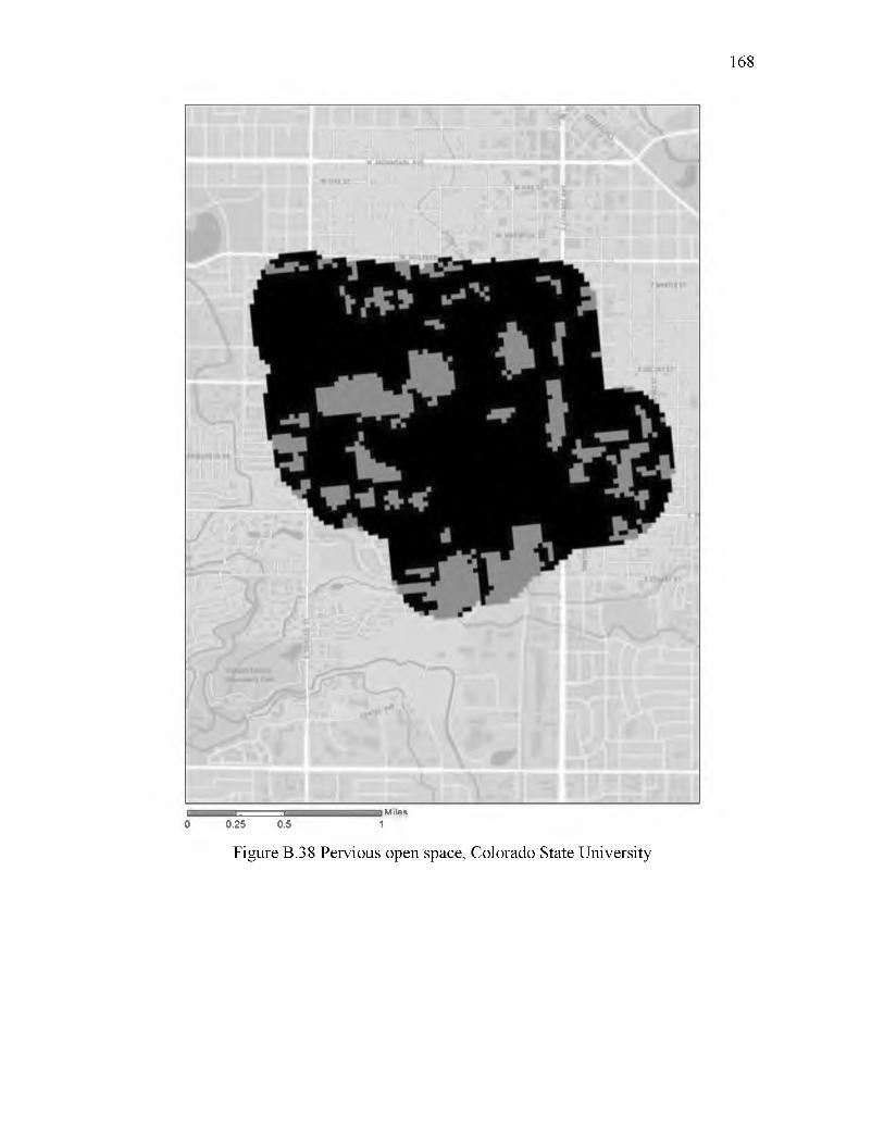
168
' i i — i M ila s
0 0.25 0.5 1
Figure B.38 Pervious open space, Colorado State University

169
Mi l es0 0.25 0.5 1
Figure B.39 The intensity of tree canopy, Colorado State University

170
i i i 1 Mi l es0 0.25 0.5 1
Figure B.40 Figure ground map, University of Connecticut

171
i i i -i Miles0 0.25 0.5 1
Figure B.41 Pervious open space, University of Connecticut
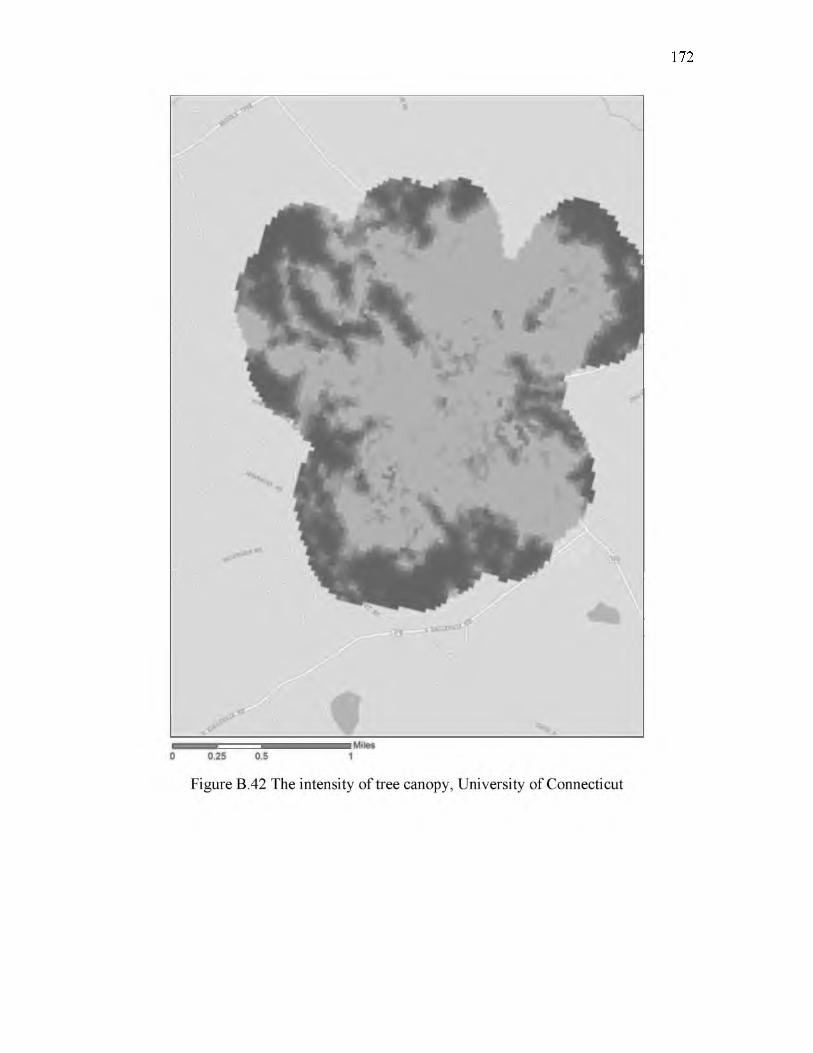
172

173
Figure B.43 Figure ground map, Cornell University
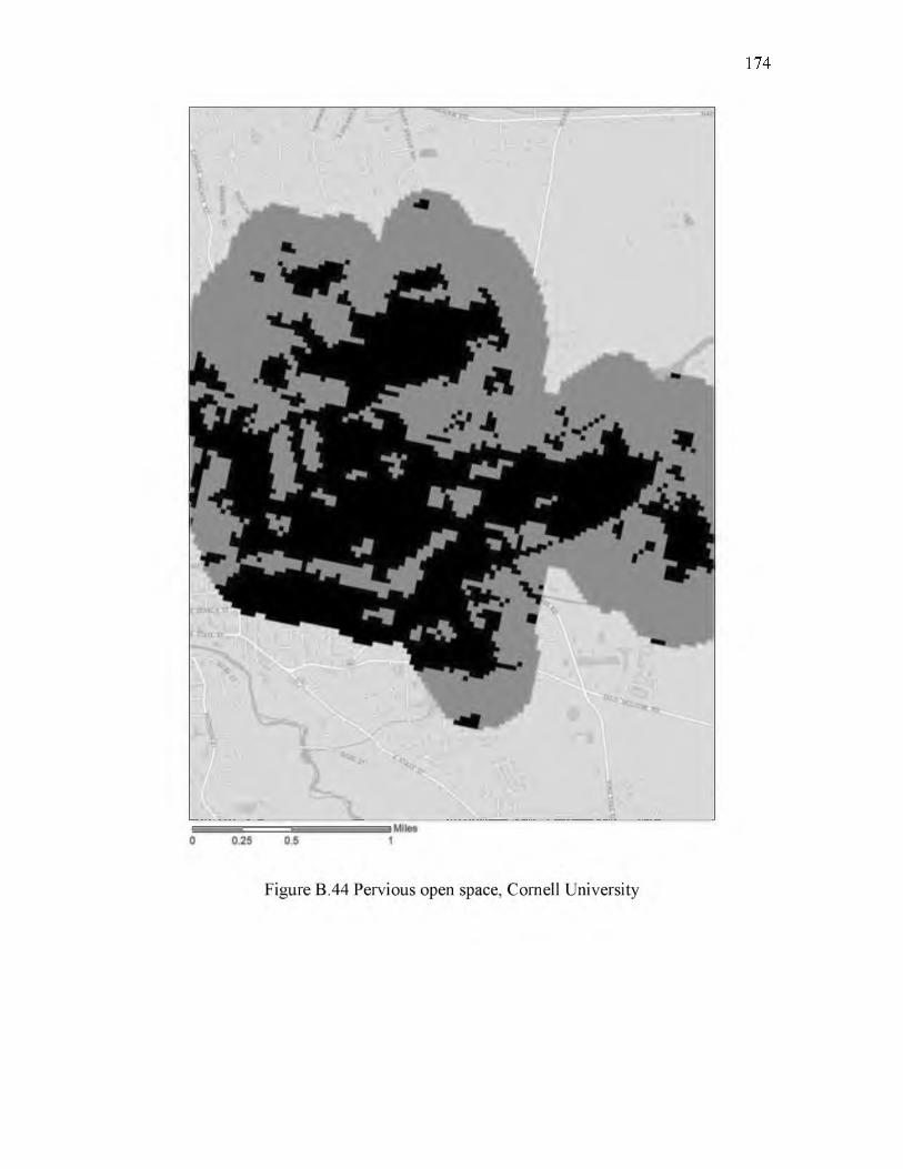
174

175
Figure B.45 The intensity of tree canopy, Cornell University

176
Figure B.46 Figure ground map, Duke University

177
Figure B.47 Pervious open space, Duke University

178
Figure B.48 The intensity of tree canopy, Duke University

179
Figure B.49 Figure ground map, University of Louisville
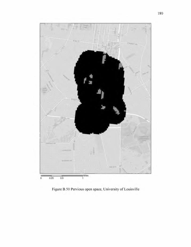
180
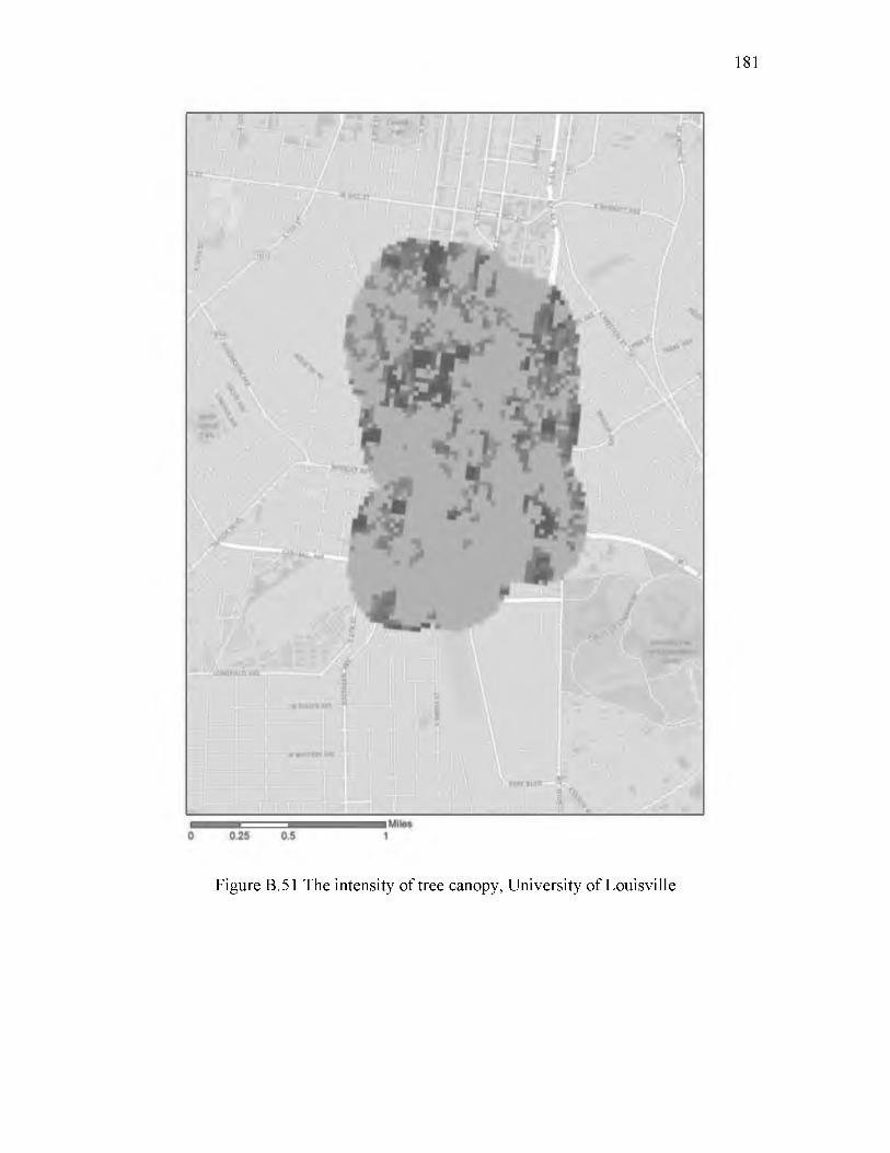
181
Figure B.51 The intensity of tree canopy, University of Louisville

182
ZTWl
!«!•i r'
- 1-•* * f->.AiI J*-<'■-••IT /
1 -r *r 1V $lv*
n'r *
0 0.25 0.5 1
Figure B.52 Figure ground map, University of Nevada
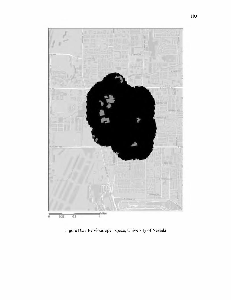
183
Figure B.53 Pervious open space, University of Nevada

184
Figure B.54 The intensity of tree canopy, University of Nevada
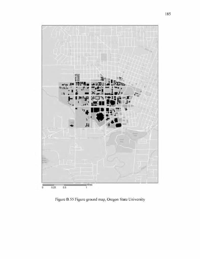
185
Figure B.55 Figure ground map, Oregon State University

186
t ■ ■ ----- 1 M ilA g
0 0.25 0.5 1
Figure B.56 Pervious open space, Oregon State University

187
Figure B.57 The intensity of tree canopy, Oregon State University

188
0.25 0.5
Figure B.58 Figure ground map, University of Tennessee
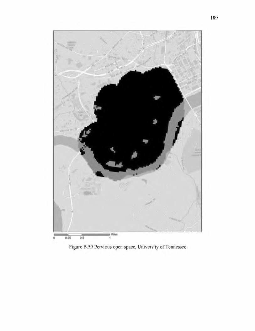
189

190
Figure B.60 The intensity of tree canopy, University of Tennessee
SELECTED BIBLIOGRAPHY
Aditjandra, P. T., Cao, X. J., & Mulley, C. (2012). Understanding neighbourhood design impact on travel behaviour: An application of structural equations model to a British metropolitan data. Transportation Research Part A: Policy and Practice, 46(1), 22-32.
Alexander, C., Ishikawa, S., & Silverstein, M. (1977). A pattern language: Towns, buildings, construction (Vol. 2). New York: Oxford University Press.
Alexander, C. (Ed.). (1987). A new theory o f urban design (Vol. 6). New York: Oxford University Press.
Alexander, C. (1979). The timeless way o f building (Vol. 1). New York: Oxford University Press.
Ariga, T. (2005). Morphology, sustainable evolution of inner-urban neighborhoods in San Francisco. Journal o f Asian Architecture and Building Engineering, 4(1), 143-150.
Atherton, A., & Giurco, D. (2011). Campus sustainability: Climate change, transport and paper reduction. International Journal o f Sustainability in Higher Education, 12(3), 269279.
Bacolod, M., Blum, B. S., & Strange, W. C. (2009). Skills in the city. Journal o f Urban Economics, 65(2), 136-153.
Banning, J. H. (1993). The pedestrian’s visual experience on campus: Informal learning of cultural messages. The Campus Ecologist, 11(1), 1-3.
Banning, J., & Bartels, S. (1993). A taxonomy for physical artifacts: Understanding campus multiculturalism. The Campus Ecologist, 11(3), 2-3.
Beatley, T. (1997). The ecology o f place: Planning for environment, economy, and community. Washington, DC: Island Press.
Belfield, C. R., & Bailey, T. (2011). The benefits of attending community college: A review of the evidence. Community College Review, 39(1), 46-68.
Bender, T. (Ed.). (1988). The university and the city: From medieval origins to the present. Oxford: Oxford University Press.
Beyer Blinder Belle Architects & Planners, (2008). Princeton Campus Plan, the Next 10 Years and Beyond. Retrieved from http://campusplan.princeton.edu/sites/campusplan.

192
Black, D. A., & Smith, J. A. (2004). How robust is the evidence on the effects of college quality? Evidence from matching. Journal o f Econometrics, 121(1), 99-124.
Black, D. A., & Smith, J. A. (2006). Estimating the returns to college quality with multiple proxies for quality. Journal o f Labor Economics, 24(3), 701-728.
Black, D., Smith, J., & Daniel, K. (2005). College quality and wages in the United States. German Economic Review, 6(3), 415-443.
Bollen, K. A. (1998). Structural equation models. In P. Armitage & T. Colton (Eds.), Encyclopedia o f biostatistics (pp. 4363-4372). Sussex, UK: John Wiley.
Bowen, N. K., & Guo, S. (2011). Structural equation modeling. Oxford: Oxford University Press.
Bowen, W. G., & Shapiro, H. T. (Eds.). (1998). Universities and their leadership. Princeton, NJ: Princeton University Press.
Boyer, E. L. (1987). College: The undergraduate experience in America. New York: Harper & Row, Publishers, Inc.
Bradley, S. M. (2009). Harlem vs. Columbia University: Black student power in the late 1960s. Urbana, IL: University of Illinois Press.
Brooks, R. (2005). Measuring university quality. The Review o f Higher Education, 29(1), 1-21.
Byrne, B. M. (2010). Structural equation modeling with AMOS: Basic concepts, applications, and programming. New York: Routledge, Tylor & Francis Group.
Cao, X., Mokhtarian, P. L., & Handy, S. L. (2007). Do changes in neighborhood characteristics lead to changes in travel behavior? A structural equations modeling approach. Transportation, 34(5), 535-556.
Casey, E. S. (2013). The fate o f place: A philosophical history. Berkeley, CA: University of California Press.
Cervero, R., & Hansen, M. (2002). Induced travel demand and induced road investment: A simultaneous equation analysis. Journal o f Transport Economics and Policy, 469-490.
Cervero, R., & Kockelman, K. (1997). Travel demand and the 3Ds: Density, diversity, and design. Transportation Research Part D: Transport and Environment, 2(3), 199-219.
Cervero, R., & Murakami, J. (2010). Effects of built environments on vehicle miles traveled: Evidence from 370 US urbanized areas. Environment and Planning A, 42(2), 400-418.
Chapman, M. P. (2006). American places: In search o f the twenty-first century campus. Westport, CT: Praeger.

193
Coltman, T., Devinney, T. M., Midgley, D. F., & Venaik, S. (2008). Formative versus reflective measurement models: Two applications of formative measurement. Journal of Business Research, 61(12), 1250-1262.
Cortes, I. C. P. (2006). Morphological analysis of the contemporary urban territory: Is it still a relevant approach?. Urban Transformations and Sustainability: Progress of Research Issues in Urbanism 2005, 95.
Coulson, J., Roberts, P., & Taylor, I. (2010). University planning and architecture: The search for perfection. Abingdon, UK: Routledge.
Coulson, J., Roberts, P., & Taylor, I. (2014). University Trends: Contemporary Campus Design. Abingdon, UK: Routledge.
Cox, B. E., & Orehovec, E. (2007). Faculty-student interaction outside the classroom: A typology from a residential college. The Review o f Higher Education, 30(4), 343-362.
Cullen, G. (1971). The concise townscape. New York: Van Nostrand Reinhold Co.
da Silva, l. C., & Heitor, t. V. (2014). Campus as a city, city as a campus: University precincts in urban context. The 7th knowledge cities world summit, 10. Estonia: Tallinn.
Daniel, K., Black, D., & Smith, J. (1997). College quality and the wages o f young men. Department of Economics, University of Western Ontario.
Darin, M. (1998). The study of urban form in France. Urban Morphology, 2(2), 63-76.
De Nisco, A., & Warnaby, G. (2014). Urban design and tenant variety influences on consumers' emotions and approach behavior. Journal o f Business Research, 67(2), 211217.
Delbanco, A. (2014). College: What it was, is, and should be. Princeton, NJ: Princeton University Press.
Disterheft, A., Caeiro, S., Azeiteiro, U. M., & Leal Filho, W. (2014). Sustainable universities-a study of critical success factors for participatory approaches. Journal of Cleaner Production, 1-11.
Dober, R. P. (1996). Campus planning. New York: Reinhold Publishing Corporation.
Duderstadt, J. J. (2000). A university for the 21st century. Ann Arbor, MI: University of Michigan Press.
Elin, N. (2012). Good urbanism: Six steps to creating prosperous communities. New York: Island Press.
Etienne, H. F. (2012). Pushing back the gates: Neighborhood perspectives on university- driven revitalization in West Philadelphia. Philadelphia, PA: Temple University Press.

194
Ewing, R., & Cervero, R. (2010). Travel and the built environment: A meta-analysis. Journal o f the American Planning Association, 76(3), 265-294.
Ewing, R., Hamidi, S., & Grace, J. B. (2014b). Urban sprawl as a risk factor in motor vehicle crashes. Urban Studies, 0042098014562331.
Ewing, R., Hamidi, S., Gallivan, F., Nelson, A. C., & Grace, J. B. (2014a). Structural equation models of VMT growth in US urbanised areas. Urban Studies, 0042098013516521.
Farr, D. (2012). Sustainable urbanism: Urban design with nature. Hoboken, NJ: John Wiley & Sons.
Fisher, B. S., & Sloan III, J. J. (Eds.). (2014). Campus crime: Legal, social, and policy perspectives. Springfield, IL: Charles C. Thomas Publisher.
Fitzgerald, R. A. & Burns, S. (2000). College Quality and the Earnings o f Recent College Graduates. Washington, DC: US Dept. of Education, Office of Educational Research and Improvement.
Fonseca, A., Macdonald, A., Dandy, E., & Valenti, P. (2011). The state of sustainability reporting at Canadian universities. International Journal o f Sustainability in Higher Education, 12(1), 22-40.
Fox, J. A., & Hellman, D. A. (1985). Location and other correlates of campus crime. Journal o f Criminal Justice, 13(5), 429-444.
Frampton, K. (1983). Prospects for a critical regionalism. Perspecta: The Yale Architectural Journal, 20, 147-162.
Franck, K. A., & Schneekloth, L. H. (Eds.). (1994). Ordering space: Types in architecture and design (Vol. 135). New York: Van Nostrand Reinhold.
Gaines, T. A. (1991). The campus as a work o f art. New York: Praeger Publishers.
Gehl, J. (1987). Life between buildings: Using public space. New York: Van Nostrand Reinhold.
Gil, J., Beirao, J. N., Montenegro, N., & Duarte, J. P. (2012). On the discovery of urban typologies: Data mining the many dimensions of urban form. Urban Morphology, 16(1), 27.
Gilderbloom, J. I., & Mullins, R. L. (2005). Promise and betrayal: Universities and the battle for sustainable urban neighborhoods. Albany, N Y : SUNY Press.
Grant, G., & Riesman, D. (1978). The perpetual dream. Reform and experiment in the American college. Chicago, IL: University of Chicago Press.

195
Greene, M., & Penn, A. (1997). Socio-spatial analysis of four university campuses: The implications of spatial configuration on creation and transmission of knowledge. In: (Proceedings) Space Syntax First International Symposium. London, UK.
Griffith, J. C. (1994). Open space preservation: An imperative for quality campus environments. The Journal o f Higher Education, 65(6), 645-669.
Haar, S. (2011). The city as campus: Urbanism and higher education in Chicago. Minneapolis, MN: University of Minnesota Press.
Hajrasouliha, A., & Yin, L. (2014). The impact of street network connectivity on pedestrian volume. Urban Studies, doi: 10.1177/0042098014544763.
Hancock, R., & Mueller, O. (Eds.). (2013). Structural equation modeling: A second course. Greenwich, CT: IAP.
Haskins, C. H. (1957). The rise o f universities, Ithaca, NY: Cornell Press.
Hillier, B. (2007). Space is the machine: A configurational theory o f architecture. Cambridge: Cambridge University Press.
Hillier, B. (2009). Spatial sustainability in cities: Organic patterns and sustainable forms. In D. Koch, L. Marcus, & J. Steen (Eds.), Proceedings of the 7th international Space Syntax symposium. Stockholm, Sweden.
Hillier, B., & Hanson, J. (1984). The social logic o f space. Cambridge: Cambridge University Press.
Hillier, B., & Iida, S. (2005). Network and psychological effects in urban movement. Spatial Information Theory, 3693(1), 475-490.
Hough, M. (1984). City form and natural process: Towards a new urban vernacular. New York: Croom Helm.
Hughes, E. (2011). Issues in Illinois college campus safety: Trends in campus crime at four-year institutions, 2005-2008. Illinois Criminal Justice Information Authority.
Hughes, R. M. (1925). A study o f the graduate schools o f America. Oxford, OH: Miami University.
Jacobs, J. (1961). The death and life o f great American cities. New York: Vintage.
Janin, H. (2008). The university in medieval life, 1179-1499. Jefferson, NC: McFarland.
Jessup-Anger, J. E. (2012). Examining how residential college environments inspire the life of the mind. The Review o f Higher Education, 35(3), 431-462.
Kenney, D. R., Dumont, R., & Kenney, G. S. (2005). Mission and place: Strengthening learning and community through campus design. Westport, CT: Praeger Publishers.
196
Kerr, C. (2001). The uses o f the university. Cambridge, MA: Harvard University Press.
Kline, R. B. (2011). Principles and practice o f structural equation modeling. New York: Guilford press.
Krier, L. (2009). The architecture o f community. Washington DC: Island Press.
Krier, R. (1979). Urban Space. London: Academy Editions.
Kubat, A. S. (2010). The study of urban form in Turkey. Urban Morphology, 14(1), 3148.
Lang, J. T. (2005). Urban design: A typology o f procedures and products. Oxford: Elsevier/Architectural Press.
Lau, L. K. (2003). Institutional factors affecting student retention. Education- Indianapolis then Chula Vista-, 124(1), 126-136.
Lefebvre, H. (1991). The production o f space. (D. Nicholson-Smith, Trans.) Oxford: Blackwell. (Original work published 1991)
Levy, A. (1999). Urban morphology and the problem of the modern urban fabric: Some questions for research. Urban Morphology, 3, 79-85.
Liu, C. (2012). Exploring the influence o f urban form on travel and energy consumption, using structural equation modeling (Doctoral dissertation). University of Maryland, College Park.
Liu, C., & Shen, Q. (2011). An empirical analysis of the influence of urban form on household travel and energy consumption. Computers, Environment and Urban Systems, 35(5), 347-357.
Long, L. D. (2014). Does it matter where college students live? Differences in satisfaction and outcomes as a function of students’ living arrangement and gender. The Journal o f College and University Student Housing, 40(2), 66-85.
Long, M. C. (2008). College quality and early adult outcomes. Economics o f Education Review, 27(5), 588-602.
Lynch, K. (1960). The image o f the city (Vol. 11). Cambridge, MA: MIT press.
Lynch, K. (1984). Good city form. Cambridge, MA: MIT press.
Marcoulides, G. A., & Schumacker, R. E. (Eds.). (2013). Advanced structural equation modeling: Issues and techniques. Oxford: Psychology Press.
Martinez, S. M., Arredondo, E. M., Roesch, S., Patrick, K., Ayala, G. X., & Elder, J. P. (2011). Walking for transportation among Latino adults in San Diego County: who meets physical activity guidelines? Journal o f Physical Activity & Health, 8(7), 898.
197
Marzbali, M. H., Abdullah, A., Razak, N. A., & Tilaki, M. J. M. (2012). Validating crime prevention through environmental design construct through checklist using structural equation modelling. International Journal o f Law, Crime and Justice, 40(2), 82-99.
Mitchell, W. J., & Vest, C. M. (2007). Imagining MIT: Designing a campus for the twenty-first century. Cambridge, MA: MIT Press.
Monks, J. (2000). The returns to individual and college characteristics: Evidence from the National Longitudinal Survey of Youth. Economics o f Education Review, 19(3), 279-289.
Moor, M., & Rowland, J. (Eds.). (2006). Urban design futures. London: Routledge.
Moudon, A. V. (1997). Urban morphology as an emerging interdisciplinary field. Urban Morphology, 1(1), 3-10.
National Survey of Student Engagement. (2013). A fresh look at student engagement. NSSE 2013 Report. Retrieved September 2015, fromhttp://nsse.iub.edu/NSSE_2013_Results/pdf/NSSE_2013_Annual_Results.pdf#page=36.
Nesbitt, K. (Ed.). (1996). Theorizing a new agenda for architecture: An anthology of architectural theory 1965-1995. Princeton, NJ: Princeton Architectural Press.
Newman, P., & Kenworthy, J. (1999). Sustainability and cities: Overcoming automobile dependence. New York: Island Press.
Norberg-Schulz, C. (1976). The phenomenon of place. In M. Larice (Ed.), Urban design reader (pp. 125-137). London: Routledge.
Oldenburg, R. (1999). The great good place: Cafes, coffee shops, bookstores, bars, hair salons, and other hangouts at the heart o f a community. New York: Marlowe.
Ostriker, J. P., Holland, P. W., Kuh, C. V., & Voytuk, J. A. (2010). A data-based assessment o f research-doctorate programs in the United States. Washington, DC: National Academies Press.
Pedersen, O. (1997). The first universities: Studium generals and the origins o f university education in Europe. Cambridge: Cambridge University Press.
Perry, D. C., & Wiewel, W. (Eds.). (2005). The university as urban developer: Case studies and analysis. Armonk, NY: ME Sharpe.
Pike, G. R. (2004). Measuring quality: A comparison of US News rankings and NSSE benchmarks. Research in Higher Education, 45(2), 193-208.
Pope, R. L., Reynolds, A. L., & Mueller, J. A. (2014). Creating multicultural change on campus. New York: John Wiley & Sons.
Ravenscroft, N. (2000). The vitality and viability of town centers. Urban Studies, 37(13), 2533-2549.

198
Raykov, T. (2000). On sensitivity of structural equation modeling to latent relation misspecifications. Structural Equation Modeling, 7(4), 596-607.
Relph, E. (1976). Place and placelessness (Vol. 67). London: Pion.
Rhodes, F. H. T. (2001). The creation o f the future: The role o f the American university. Ithaca, NY: Cornell University Press.
Riginos, C., & Grace, J. B. (2008). Savanna tree density, herbivores, and the herbaceous community: Bottom-up vs. top-down effects. Ecology, 89(8), 2228-2238.
Roberts, J., & Styron, R. (2010). Student satisfaction and persistence: Factors vital to student retention. Research in Higher Education Journal, 6(3), 1-18.
Rodin, J. (2007). The university and urban revival: Out o f the ivory tower and into the streets. Philadelphia, PA: University of Pennsylvania Press.
Rossi, A., & Eisenman, P. (1982). The architecture o f the city. Cambridge, MA: MIT Press.
Rutt, C. D., & Coleman, K. J. (2005). Examining the relationships among built environment, physical activity, and body mass index in El Paso, TX. Preventive Medicine, 40(6), 831-841.
Rowe, C., & Koetter, F. (1983). Collage city. Cambridge, MA: MIT press.
Saadatian, O., Dola, K., Salleh, E., & Tahir, O. M. (2011). Identifying strength and weakness of sustainable higher educational assessment approaches. International Journal of Business and Social Science, 2(3), 137-146.
Scheer, B. C. (2010). The evolution o f urban form: Typology for planners and architects. Chicago, IL: APA Planners Press.
Schuetz, P. (2005). UCLA community college review: Campus environment: A missing link in studies of community college attrition. Community College Review, 32(4), 60.
Sima, Y., & Zhang, D. (2009). Comparative precedents on the study of urban morphology. In Proceedings o f the 7th International Space Syntax Symposium,Stockholm: KTH (pp. 103-1).
Sloan, J. J. (1994). The correlates of campus crime: An analysis of reported crimes on college and university campuses. Journal o f Criminal Justice, 22(1), 51-61.
Spirn, A. W. (1985). The granite garden: Urban nature and human design. New York: Basic Books.
Steiner, F. (2011). Landscape ecological urbanism: Origins and trajectories. Landscape and Urban Planning, 100(4), 333-337.

199
Steinmetz, C. A. (2009). Universities as place: An intergenerational perspective on the experience o f Australian university students (Doctoral dissertation), University of New South Wales Sydney, Australia.
Strange, C. C., & Banning, J. H. (2001). Education by design: Creating campus learning environments that work. San Francisco, CA: Jossey-Bass.
Stuart, D. L. (1995). Reputational rankings: Background and development. New Directions for Institutional Research, 1995(88), 13-20.
Temple, P. (2008). Learning spaces in higher education: An under-researched topic. London Review o f Education, 6(3), 229-241.
Thelin, J. R., & Yankovich, J. (1987). Bricks and mortar: Architecture and the study of higher education. Higher education: Handbook o f theory and research, 3(1), 57-83.
Thilagam, N. L. (2015). Integrated land use development for green campus. In W. Leal Filho, N. Muthu, G. Edwin, & M. Sima (Eds.), Implementing campus greening initiatives (pp. 203-214). Switzerland: Springer.
Toor, W., & Havlick, S. (2004). Transportation and sustainable campus communities: Issues, examples, solutions. New York: Island Press.
Trache, H. (2001). Promoting urban design in development plans: Typo-morphological approaches in Montreuil, France. Urban Design International, 6(3), 157-172.
Trancik, R. (1986). Finding lost space: theories o f urban design. New York: John Wiley & Sons.
Turner, A. (2007). From axial to road-center lines: A new representation for space syntax and a new model of route choice for transport network analysis. Environment and Planning B: Planning and Design, 34(3), 539-555.
Turner, P. V. (1984). Campus: An American planning tradition. Cambridge, MA: MIT Press.
Turner, T. (2005). Garden history: Philosophy and design 2000 BC-2000 AD. London: Routledge.
U.S. News & World Report (2015). How U.S. News Calculated the 2015 Best Colleges Rankings. Retrieved September 2015, from http://www.usnews.com/education/best- colleges/articles/2014/09/08/how-us-news-calculated-the-2015-best-colleges- rankings?page=1
Ullman, J. B., & Bentler, P. M. (2003). Structural equation modeling. New York: John Wiley & Sons, Inc.

200
Wigmore, A., & Ruiz, M. (2010). Sustainability assessment in higher education institutions. The stars system. Ramon Llull Journal o f Applied Ethics, 1(1), 25.
Yaylali-Yildiz, B., Czerkauer-Yamu, C., & £il, E. (2014). Exploring the effects of spatial and social segregation in university campuses, IZTECH as a case study. Urban Design International, 19(2), 125-143.