The Monetary Sector under a Currency Board Arrangement ... · The Monetary Sector under a Currency...

The Monetary Sector under a Currency BoardArrangement: Specification and Estimation

of a Model with Estonian Data*

Rasmus Pikkani**

Tallinn 2000

Modelling work on Estonian data indicates that external financing of the privatesector has strong impact on domestic demand, which implies that valuable insightsmay be gained in this case from understanding the behavioural relationships in themonetary sector. The current paper provides a theoretical analysis of the monetarysector under a currency board regime and applies specification tests to Estonian data.As a final product, empirical equations for average lending rate, loans provided to theprivate sector and money demand are estimated. While estimations herein usemonthly data, quarterly modifications of the model will be inserted into Eesti Pank’squarterly macromodel in the future.

*This study has been partially conducted during the author’s stay at the Bank of Finland,Institute for Economies in Transition (BOFIT) and was first published in the BOFIT Onlineseries.

**I would like to thank Iikka Korhonen, Jukka Pirttilä and Martti Randveer for their help andvaluable recommendations. Comments on the present text are welcome.

Author’s e-mail address: [email protected]

The views expressed are those of the author and do not necessarily represent the officialview of Eesti Pank.

Contents

1. Introduction ____________________________________________________ 3

2. Overview of an orthodox currency board arrangement and Estonia’smonetary system ________________________________________________ 5

3. Specification of the Estonian model’s structure ________________________ 6

Demand for bank credit ________________________________________ 12

Supply of bank lending_________________________________________ 13

Money demand _______________________________________________ 14

4. Empirical estimation ____________________________________________ 15

Background__________________________________________________ 15

Estimation results _____________________________________________ 19

5. Concluding remarks_____________________________________________ 23

Glossary __________________________________________________________ 25

Appendix I. Evolution of Eesti Pank’s monetary policy operational framework___ 27

Appendix II. Results from Granger Causality Test and VAR regressions ________ 29

Appendix III. Figures ________________________________________________ 33

Appendix IV. Statistical protocols ______________________________________ 37

References_________________________________________________________ 47

3

1. Introduction

Over eight years ago, Estonia introduced its own currency, the kroon. It has conductedindependent monetary policy ever since. At the time of the currency reform in 1992,Estonia had 42 commercial banks.1 Today, bankruptcies and intense consolidationhave winnowed the field to six banks and a branch office of a foreign bank. The twolargest banks control over 80% of the market. This consolidation occurred inanticipation of major market expansion, and indeed, between 1993 and 1999, totaldeposits rose from EEK 2.5 billion to EEK 28 billion, while loans provided to theprivate sector rose from EEK 1.3 billion to EEK 27 billion. Nominal GDP,meanwhile, increased only 2.5 times, which reflects high growth rates in monetisationof the economy and relaxation of liquidity constraints in the real sector of theeconomy.

The banking sector has likely played an important role in generating domestic demandby relaxing liquidity constraints faced by the private sector. This assumption findssupport in demand-side models of the Estonian data. These models often reveal thatthe amount of loans provided to the private sector or domestic lending rates have asignificant impact on variables reflecting domestic demand and propensities toimport.2

The objective of the current paper, therefore, is to develop an econometric model ofthe Estonian monetary sector. In the future, the estimated model will be modified tobe used in the aggregated quarterly macroeconometric model currently underconstruction by economists at Eesti Pank, Estonia’s central bank. Nevertheless, theobjective of the current work is not merely to generate empirical estimates, but also toanalyse developments in the monetary sector to get a reliable specification of themodel. Thus, monthly data are used in the current analysis. Moreover, the currentquarterly time series (23 observations from the beginning of 1994 until Q3 1999) istoo short to provide meaningful empirical estimates. The samples from 1994 and early1995 also fall into an unstable period when annual inflation exceeded 30% and outputcontracted.

Because Estonia uses a currency board arrangement (CBA) and therefore lacksindependence in determining its monetary policy, foreign impacts deserve specialdiscussion. Herein, two alternative specifications for foreign capital supply regimeswill be tested.

Macroeconomists earlier found little reason to analyse factors determining bank creditdemand (Fase 1995, Rother 1999), since they are mainly interested in overalleconomic activity. They devote effort to discerning how financial intermediationpromotes growth, rather than how economic activity (or expectations) affect demandfor external financing. Thus, it is difficult to find a widely accepted economic theoryon which to base the current modelling exercise.

1 Eesti Pank (1999a, p. 44)2 Sepp, Pikkani and Rell (1999); Sepp (1999)

4

Fortunately, there are several ad hoc works analysing the monetary sector and theseprovide great help in specifying equations for domestic loans market.

Olexa (1998) has estimated a monetary sub-model for the Slovak Republic using astructure of dependent variables quite similar to the one used in the current paper.Although he gives no theoretical foundation for his reasoning, he does estimate thenominal amount of bank credit provided to the private sector as a function of nominalGDP, the real interest rate on credit (deflated with current investment price deflator)and credit provided to government. The credit function is estimated as a functionseparate from interest rates and the money stock and assumes no simultaneity.

Catao (1997) specifies supply and demand equations for bank credit using Argentinedata to determine whether demand or supply-side factors caused a contraction indomestic bank lending. His work is particularly relevant as it concerns the monetarysector under a currency board arrangement. He specifies the long-run supply equationas a function of lending capacity (defined as deposits – liquidity requirements – cashin vault + own capital + net foreign liabilities) and the average lending rate. Indynamic equations, supply is defined as a function of change in lending capacity,change in interest rate and change in the share of problematic loans in bank portfolios.The long-run demand of bank credit is estimated as a function of nominal GDP andthe average lending rate. The change in demand is specified as a function of theexpected change in nominal GDP, change in lending rate, and the level of structuralunemployment. Both dynamic supply and demand equations were accompanied witherror-correction terms derived from the long-run equations. The estimated functionsreveal that the slow recovery in banking credit in Argentina was caused mainly by thebehaviour of the domestic non-banking sector, not supply-side restrictions.

The paper is structured as follows. In section 2 we briefly discuss an orthodoxcurrency board arrangement and contrast it with the system used in Estonia. Section 3gives possible specifications of the monetary sector model’s structure withspeculation on possible changes in foreign debt capital supply regimes. Section 4presents tests for accuracy of various specifications and an empirical estimation of themodel. Section 5 concludes and offers some future perspectives.

5

2. Overview of an orthodox currency board arrangement andEstonia’s monetary system

Before attempting an analysis of Estonia’s monetary sector, we require a briefcomparison of the differences between orthodox currency board systems and theEstonian system. An orthodox currency board arrangement (CBA) is an exchange ratearrangement whereby the monetary authority stands ready to exchange local currencyfor another (anchor) currency at a fixed exchange rate without quantitative limits.(Korhonen 1999). To be reliably ready to supply any amount of foreign currency ondemand, orthodox currency boards call for a 100% backing of emitted domesticcurrency (or the total domestic liabilities of the domestic monetary authority) withforeign exchange reserves. 100% backing implies 100% technical or non-politicalcredibility of the stated peg, since there is no possibility that the monetary authoritywill run out of reserves. Of course, if the monetary authority is not 100% politicallyindependent or is concerned with issues other than foreign exchange operations at astated exchange rate, the possibility that the peg will not hold arises.3 To avoid thisrisk, a politically independent monetary authority runs the CBA and is invested withthe sole responsibility of carrying out demanded foreign exchange operations. Fullbacking of the domestic base money and full convertibility at a fixed exchange rateassures a totally endogenous base money supply. This basic specification of themonetary system under an orthodox CBA assures automatic sterilisation of excessliquidity. Assuming a credible exchange rate peg, any changes in money demand(other things being equal) will be accompanied by changes in base money and bycorresponding changes in foreign exchange reserves.

With the CBA and 100% backing, use of one of the most common monetary policyinstruments is restricted to excess reserves, ie the amount of reserves exceeding themonetary base at the disposal of the monetary authority. Typically, this means theautomatic lender-of-last-resort facility or discount window.

The currency board system in 1992 was introduced in conjunction with a newcurrency. The Estonian kroon (EEK) was pegged to the Deutsche Mark (DEM) at arate of one mark to eight kroons. As a result, Eesti Pank’s main monetary policyinstrument is continuous and immediate participation in the spot foreign exchangemarket at the fixed exchange rate (Lättemäe and Randveer 2000). To support smoothoperation of the foreign exchange market, there are no restrictions on capital accounttransactions. This can be interpreted as an unlimited foreign exchange window wheretransactions of buying and selling foreign currencies against reserve currencies areinitiated by commercial banks (Lepik 1999).4

3 This includes concern over the real sectors’ ability to cope with external shocks. In the event of asharp decline in international competitiveness caused by irresponsible fiscal policy or a foreignproductivity shock, adjustments through prices can take a long time and carry great costs. A politicallydependent monetary authority may find devaluation an expedient means to speed up recovery fromsuch a shock.4 There are no spreads between buying and selling rates of euro or other EMU currencies.

6

Eesti Pank also uses several other monetary policy instruments, which is why its CBAis sometimes referred to as a “currency board-like” system. The most importantmonetary policy instrument here is the required reserves ratio.5 A fixed exchange rateand reserve requirement influence the monetary sector indirectly through increasedcosts of financial intermediation.6 Eesti Pank’s other instruments include remunerateddeposit facilities for commercial banks and auctions of certificates of deposits.7 EestiPank also conducts banking supervision, bank licensing, acts as an interbank clearingand settlement centre, and provides the organisational and legal framework for theinterbank money market.

The CBA framework bars Eesti Pank from effective conduct of monetary policy tosmooth shocks in the monetary sector. The central bank can help the Estonian bankingsector by improving the legal framework and market mechanisms to better enable thebanking sector to cope with large external and internal shocks.

3. Specification of the Estonian model’s structure

In recent decades, economists have been engaged in an active debate on theendogeneity of the money stock. Endogenous money theories vary widely withrespect to the period of analysis, as well as with respect to factors determining theendogeneity of money, the degree of endogeneity, and the nature of direction ofcausality between economic activity, bank lending, price levels, and the money stock(Niggle 1991).

In Estonia’s case, the fundamental cause of endogeneity in monetary sectoraggregates is the currency board arrangement and its consequent lack of control overforeign capital flows. If we assume perfect information, then domestic interest ratesunder a credibly pegged exchange rate should converge with anchor currency rates.Interest rate convergence reflects higher integration of international financial marketswhere different financial assets become better substitutes and capital tends to seek outthe highest possible risk-adjusted returns (Fase 1999, pp 83–95).

Under a currency board arrangement, domestic interest rates should theoreticallyequal foreign interest rates plus domestic economy risk premium. If the domesticeconomy is small in relation to overseas economies and has low accumulated(foreign) debt, we can assume that in the long-run risk premium for foreign credit willnot depend on amounts lent and all reasonable amounts demanded will be offered at arate equal to foreign interest rates plus a risk premium. That risk premium, in turn, is afunction of domestic fundamental variables that reflect the risk of the domesticeconomy. Intuitively, this premium is likely to be fairly stable over the short run.

5 Also composition of liabilities facing reserve requirements, composition of reserves assets andremuneration.6 And not directly through reduction of banking sector lending resources as is commonly claimed instandard textbook discussions on closed economies.7 A table describing the evolution of Eesti Pank monetary policy is presented in Appendix I.

7

An alternative, and perhaps more elegant, way to explain formation of domesticinterest rates applies the concept of uncovered interest rate parity, equalising risk-adjusted expected returns across countries. Here the difference between domestic andinternational nominal interest rates equals foreign interest rates plus expecteddevaluation plus risk premium. This risk premium, in turn, can be divided into twoparts: (1) the premium covering exchange rate risks, and (2) the country-specific riskpremium covering risks from possible lack of liquidity in the system, term structureand default risk (Fase 1999, pp 83–95).

It is reasonable to assume that over the long run the above descriptions hold and thatforeign capital is elastic. However, historical data are also likely to show that theabove descriptions do not hold over a shorter period of time and that in the short runthe foreign capital supply can sometimes be non-elastic. Now consider the Estoniancase. Estonia is a tiny country and any amounts borrowed from international financialinstitutions most likely constitute a tiny share of a large lender’s total loan portfolio.In the event of financial turmoil in emerging markets, international institutions mayfind it more expedient and cheaper to simply freeze lending to small countries, ratherthan bother to analyze possible linkages between turmoil elsewhere in the world andthe local economy. This effect may be amplified by the fact that countries are oftengrouped together rather than considered by individual states. Moreover, some foreigninstitutions may forego analysis altogether and simply copy the actions of others withgood records.

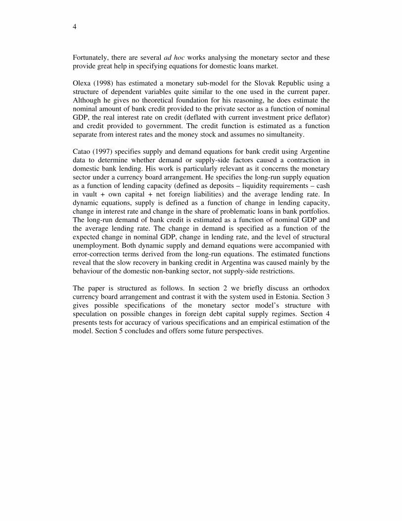
Figure 1 indicates periods of non-elastic foreign capital supply. It should bementioned here, however, that after the banking sector consolidation and the radicalchange in ownership of domestic banks during summer 1998, credible interbankmoney market rates were scarce.8 After consolidation, the country’s two largest bankscontrolled around 80% of the domestic banking sector and the new owner structureassured credible credit channels outside the domestic interbank money market. This iseasily notable in the decline in overnight interbank lending amounts to nearly zeroafter summer 1998. An obvious indicator of the interbank money market is the TallinnInterbank Offer Rate (TALIBOR), but it has problems similar to overnight moneymarket and the time series are limited.9 Moreover, TALIBOR rates are not theaverage price of money actually lent, but the market average of quotations on whatbanks on the market are obliged to supply to others on the market. From Figure 1 itcan be seen that the sharp increase in overnight money market rates in 1997 coincidedwith a rise in the TALIBOR. This gives us some confidence to assume thatmovements in overnight interest rates over the period with low turnover may beaccurate, as these movements are consistent with TALIBOR movements.

8 For detailed information about banking sector consolidation see Eesti Pank (1999b, p 40–41).9 Eesti Pank started fixing TALIBOR and TALIBID quotations after January 9, 1996. The five largestbanks on the market were listed and periods quoted were 1 week, 1 month and 3 months (Eesti Pank1996 p 7–8). After September 1998, because banking sector consolidation had reduced the number ofbanks to three and maximum sum banks had to deliver on quoted rates had increased from EEK 1million to EEK 10 million (Eesti Pank 1998 p 5). In February 1999, Svenska Handelsbanken andMerita Bank Plc. Tallinn branch were added to the list and a new time-structure of quotation wasintroduced. New periods quoted are 1 month, 2 months, 3 months, 6 months, 9 months and 12 months(Eesti Pank 1999c p 6).

8

Figure 1. Key market rates and turnover on overnight interbank money market.

-10%

-5%

0%

5%

10%

15%

20%

25%

94:01 94:07 95:01 95:07 96:01 96:07 97:01 97:07 98:01 98:07 99:01 99:07 00:01

0

1000

2000

3000

4000

5000

6000

7000

8000turnover on overnight money market (mln kroon, right scale)LIBOR_DEM_3MTALIBOR_3Minterbank overnight

Nevertheless, it remains tricky to specify from that figure exactly when the supply offoreign capital was restricted. Some additional figures may help this decision. Figure2 presents a plot of the difference between the average domestic lending rate (IL_AV)and the 3month London Interbank Deutsche Mark Offer Rate (LIBOR_DEM_3M).The trend should present a possible proxy for developments in total domestic riskpremia (including country risk, banking sector risk and entrepreneur’s risk). There isan observable clear decline in the long run as compared to the temporary upwardpressures between the end of 1997 and beginning of 1999. As the overall long-rundecline becomes more pronounced, the exact period of temporary upward pressure isharder to detect.

Figure 3 presents the difference between average domestic deposit rate (ID_AV) andLIBOR_DEM_3M. This difference should reflect the additional price commercialbanks are ready to pay to attract domestic deposits. A sharp increase in this difference,therefore, should reflect higher competition for domestic deposits, which in turnshould indicate restrictions on foreign capital supply. Competition for domesticdeposits can increase deposit rates to abnormally high levels only in situationsinvolving problems with external financing (otherwise, banks will resort to cheapersources abroad).10 The long-run decline is easily noticeable here, but the increase indomestic interest rates at the end of 1997 is even more distinct. Figure 2 broadlysupports Figure 1 findings using overnight and interbank 3month offer rates.

These figures present the period between September 1997 and April 1999 whendomestic financial institutions found it hard to attract foreign capital in the amountsdemanded. During this period, domestic interest rates were driven not only by foreigninterest rates and reasonable risk premium, but also by adjustments in the supply anddemand of domestic bank credit. Precise determination here is problematic. Forexample, a broad determination may include periods when constrained foreign capital

10 Another possibility is heavy competition between Hansapank and Ühispank for the title of the largestcommercial bank in Estonia.

9

supply had upward pressure while low bank credit demand placed a downwardpressure on interest rates. The sum effect would then be close to zero.

Figure 2. Difference between lending rate and 3month DEM LIBOR.

0.05

0.10

0.15

0.20

0.25

1994 1995 1996 1997 1998 1999 2000

IL_AV-LIBOR_DEM_3M

0.4643352599-0.08654128303*LOG(@TREND)

Figure 3. Difference between deposit rate and 3month DEM LIBOR.

0.00

0.02

0.04

0.06

0.08

1994 1995 1996 1997 1998 1999 2000

ID_AV-LIBOR_DEM_3M

-0.03026006974*LOG(@TREND)+0.1433581047

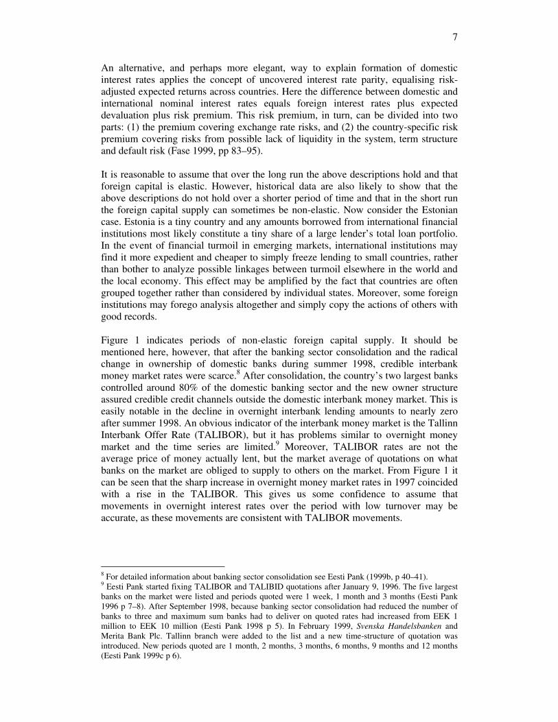
The figures may also reflect domestic constraints on foreign capital flows. Forexample, it is reasonable that commercial banks might find it relatively more time-consuming and costly to expand equity than to attract (foreign) debt flows. If thisassumption holds, then banks may find it hard to expand foreign liabilities in line withincrease in credit demand because of the required capital adequacy ratio. Figure 4,however, shows that even during the period of fastest loan portfolio growth (growthrates reaching 100% per year!) commercial banks found ways to expand equity almostin the line with the loans outstanding. The banking sector’s average capital adequacyconsistently stood more than 2 percentage points above the required level.

10

Figure 4. Capital adequacy and loan portfolio growth rates.

-0.2

0.0

0.2

0.4

0.6

0.8

1.0

1.2

0.06

0.08

0.10

0.12

0.14

0.16

0.18

96:01 96:07 97:01 97:07 98:01 98:07 99:01 99:07 00:01

loan portfolio growth (annual)capital adequacy (right scale)capital adequacy normative (right scale)

According to analysis of changes in the nature of foreign capital supply, the modelmust be specified for two periods, the first covering the theoretically more convenientlong-run condition with perfectly elastic foreign capital supply and the second forperiods with restrictions on foreign debt capital supply. There may also exist a third,intermediate period, where foreign debt capital supply is not zero and when the priceasked depends positively on the amounts lent. It seems more likely, however, thatentrance to the environment with a constrained foreign capital supply is faster andsharper than movement back to elastic supply. These possible movements of curves offoreign debt capital supply related to entrance or exit from crisis situations arepresented in Figure 5.

Before further specification, it is important to point out that, if, in the long run, thereis no intuitive difference between the supply of foreign debt capital and loan supplyfrom the domestic banking sector, then a difference arises with constrained foreigncapital supply. Let’s consider a “normal” situation, wherein all amounts of creditdemanded by the non-banking sector will be supplied by commercial banks or directlyfrom abroad at interest rates determined by anchor currency interest rates and riskpremia. In this situation, the banking sector will have no problem financing lendingby foreign debt flows. Competition, moreover, will assure proper domestic interestrates for private sector.

11

Figure 5. Supply of foreign debt capital during normal and restricted periods.

0

5

10

15

20

5 10 15 20 25 30 35 40

Foreign debt / foreign capital supply

Inte

restra

tes

Supply 1Supply 2

Demand

Supply 3

In the case of shocks, the supply of foreign debt capital can be seriously constrainedso the supply of new foreign loans to domestic financial intermediaries can get closeto zero. In these situations, the supply of foreign debt capital (essentially zero) andbank credit supply are two clearly distinguishable functions. Here, the traditionalmodel of a small open economy is inappropriate. An information problem may violatethe assumption of free and effective capital movements.

In the event of shocks (assuming no changes in bank credit demand), banks will findthemselves in a situation where they are involved in intermediation of a good that isscarce in the economy. Here the usual market forces kick into action so the amount ofloans with corresponding interest rates will be derived by the supply and demandfunction. The supply of bank credit will not be necessarily frozen, however, as bankscan optimise their asset structures to earn extra profit. Here, different monetarytransmission channels will be more pronounced (especially “credit channels”)11 asmost of them are related to problems with information. Indeed, the informationproblem becomes more critical as interest rates increase.

Without specifying the exact form and content of supply and demand equations, long-run (or normal situation) relationships may be specified as follows:12

(1.1) ( ),...F,,,..., * ririii =(1.2) ( ),...,...,..., YiLLL DDS ==(1.3) ( ),...,...,,..., YiMM DD π=

Under this specification domestic interest rates do not depend on demand variablesand bank credit demand interest rates are given exogenously.

11 For a closer description of monetary transmission channels, see Mishkin (1996) or Bernanke andGertler (1995).12 See Glossary.

12

For the periods with restricted supply of foreign capital, interest rates belong to thesame system with supply and demand equations as the adoption variable. The systemcan be specified as follows:

(2.1) ( ),......,iLL SS =(2.2) ( ),...,...,..., YiLL DD =(2.3) DS LL =(2.4) ( ),...,...,,..., YiMM DD π=

For explicit specification of the system, the motivation underlying supply and demandof different monetary aggregates needs explaining.

Demand for bank creditDemand for bank credit is the outcome of several economic indicators and estimatedfuture developments. Most are related to expected future developments in profits andcash flows. For example, if an increased demand for a firm’s production is expected,additional investments will be needed. One way to finance investment, obviously, isbank credit. Also, according to simple life cycle models for households, if estimatesabout future incomes change, the optimal consumption path will change and the needto consume during the current period will change as well. To increase consumptiontoday in correspondence with expected future incomes, external financing is needed.

It is generally difficult to find good time series for expected developments in incomesor turnovers, so the current economic situation must be used as possible indicator ofattitudes on future developments. Available indicators that reflect the currenteconomic situation, macroeconomic stability and certainty are GDP, inflation,unemployment, and the proportion of non-performing loans (a higher proportionreflects current problems in the economy or an overestimation of growth prospects inthe past).13

Long-run demand for real bank credit will be specified as a function of real GDP(scale variable), real lending rate (ir) (or separately nominal lending rate (i) andinflation (π) or inflation expectation (πe))14 and the open vector of variables reflectingconfidence and certainty σ.

( )σπ ,,, RGDPiLL DD =

In the short run, the demand for bank credit should depend broadly on the samevariables. Additionally, a certain amount of asymmetry of processes may also beintroduced. The appropriate way to introduce short-run asymmetry is througheconomic activity when we wish to estimate stock of loans outstanding (as opposed tonew loans provided), because loans are usually non-recallable in the short run. During

13 Figures with developments in most important variables are presented in Appendix V.14 During rapidly falling inflation, accurate estimates of real interest rates are hard to derive. Realinterest rates are determined by deflating nominal rates according to inflation expectations.

13

a period of rapid economic growth, demand for stock of loans outstanding willincrease faster than it is possible to reduce the stock of loans outstanding during aneconomic recession.

There are also additional restrictions on borrowing by households. As we live in aworld with asymmetric information, private agents are likely to have betterinformation about their future prospects than commercial banks. To cope with thisproblem, clients must provide additional information. If the client is a private person,the information used to determine creditworthiness is typically current wage income.This does not mean that wage income is the sole supply-side factor. Actually, it is alsoa demand-side factor, because repayment of a loan starts usually shortly afterborrowing and needs extra funds from personal budget.

Supply of bank lendingIn “normal” cases, bank credit supply is assumed to be totally elastic meaning that allamounts demanded by non-banking sector at a given price will be supplied. Thisrelationship relies on assumption of totally passive banking sector, which can attractforeign debt capital in all reasonable amounts at given interest rates and risk premia.

During the periods of constrained foreign capital supply, however, banks cannotafford to be totally passive, because they must supply a good that is scarce. In thesecases, the limited amount of available credit (or purchasing power) in the economyallows banks to raise their lending rates and earn extra profit. Another motivation forbanking sector activity during these periods is the fact that during financial distressother problems with the economy are likely to emerge. For example, asset prices maycollapse over uncertainty about the future or clients may have problems with loanrepayment. To avoid or minimise losses from loans related to projects with increaseduncertainty, banks must temporarily alter their normal lending behaviour.

Under situations of restricted supply of foreign debt capital, the supply of bank creditcan be specified as function of interest rates (i) and (constrained or fixed) resourcesfor lending activity (LR). Additional information about the quality loan portfolios φcan be used as well.

( )φ,, LRiLL SS =

Specification of the variable reflecting resources for lending activity during a foreigndebt capital supply shock is quite crucial. If we assume that money demand dependspositively on deposit rates, then money supply (which is fully determined by demandfor money under a CBA) should be included into the simultaneous system ofequations. It will have a role in determining the equilibrium interest rate during shockperiods as it is a component of lending resources (LR). There are several argumentsagainst this in the Estonian case and they will be introduced in the next section.

In any case, if we assume that money has to be included into this system, then theonly dynamics in LR during shock periods will come from money supply. In themeantime, however, this dynamic will depend on interest rates, which, in turn, dependon the bank credit supply function. Here, changes in the money supply during a shock

14

period can originate from the current account (as we still have free trade) or frominvestments from capital account (as we assume constraints on the supply of foreigndebt capital only).

Money demandAs mentioned, the functional form of money demand is crucial in specification of thefull system. Works dealing with money demand usually assume that economic agentscan choose between at least two types of liquid assets.15 One, of course, is money andthe second is usually securities. The underlying idea is that if the return from moneygets too low (or holding of money gets too costly), it may be profitable to changemoney savings to securities or just decrease average money holdings to buy securities.This specification needs to fulfil two conditions. First, there must exist alternativeassets that are highly liquid, but carry low risk, eg government bonds. Second, thetransaction cost of switching assets must be low. In the Estonian case, there are noclose substitutes for money. The closest asset alternative to money is perhaps equity,16

but even so, equity carries higher risk in exchange for a potentially higher averageexpected return. In this sense, equity is not a very close substitute for money.

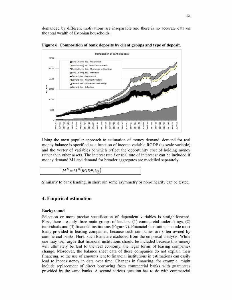
A lack of close substitutes for money may cause a situation where aggregate moneydemand ceases to depend on interest rates, because there are no alternative ways toaccumulate wealth other than time or savings deposits. A change in interest rates mayresult shifts between money aggregates (demand, time and savings deposits) or micro-level changes between banks as a result of competition, but not necessarily shiftsbetween money and other assets. The composition of domestic bank deposits ispresented in Figure 6. Note that the importance of time deposits grows constantly. Inthe beginning of 1993 M117 made up close to 90% of M2.18 At end-1999, M1 was lessthan 60% of M2 (see also Appendix III).

According to the above, there are many different processes going on simultaneouslybehind formation of aggregate money demand. It follows that demand for money canbe divided roughly into two (quantitatively indistinguishable) parts. The first is thestandard demand for money as demand for means of exchange and carrier ofpurchasing power. The second motivation is demand for money as an asset allowingaccumulation of wealth.19 If processes from the first motivation are theoretically easyto model, modelling the second motivation is far harder, since the quantities of money

15 Laidler 1993 and Sriram 1999 provide excellent coverage of developments in money theory.16 This holds for an average economic agent. Several money mutual funds exist, but entry barriers arequite high and earnings do not differ significantly from time deposit rates. Once Estonia had numerousopen investment funds, but most cancelled operations after the near-collapse of the Tallinn stockexchange at the end of 1997. A third alternative is to deposit money abroad, but this is out of the scopeof an average domestic economic agent (ie individuals and small business are put off by the hightransaction costs, but larger companies routinely use foreign deposit accounts for liquidity managementand similar purposes).17 Defined as sum of cash in economy and demand deposits in commercial banks.18 Defined as M1 + time and saving deposits.19 According to the Statistical Office of Estonia, the average total income per member of household in1999 was 2,000 kroons. At the same time, the average amount of demand deposits per residentaveraged around 3,700 kroons. The amount of time and saving deposits averaged around 2,700 kroons,or 3.2 times the monthly average income (in 1998, respectively, 1,900 kroons, 3,100 kroons, 2,500kroons and 2.9 times).

15

demanded by different motivations are inseparable and there is no accurate data onthe total wealth of Estonian households.

Figure 6. Composition of bank deposits by client groups and type of deposit.

Composition of bank deposits

0

5000

10000

15000

20000

25000

3000031

.01.

93

30.0

4.93

31.0

7.93

31.1

0.93

31.0

1.94

30.0

4.94

31.0

7.94

31.1

0.94

31.0

1.95

30.0

4.95

31.0

7.95

31.1

0.95

31.0

1.96

30.0

4.96

31.0

7.96

31.1

0.96

31.0

1.97

30.0

4.97

31.0

7.97

31.1

0.97

31.0

1.98

30.0

4.98

31.0

7.98

31.1

0.98

31.0

1.99

30.0

4.99

31.0

7.99

31.1

0.99

31.0

1.00

30.0

4.00

mln

.EE

K

Time & Saving dep. - Government

Time & Saving dep. - Financial Institutions

Time & Saving dep. - Commercial undertakings

Time & Saving dep. - Individuals

Demand dep. - Government

Demand dep. - Financial Institutions

Demand dep. - Commercial undertakings

Demand dep. - Individuals

Using the most popular approach to estimation of money demand, demand for realmoney balance is specified as a function of income variable RGDP (as scale variable)and the vector of variables γ, which reflect the opportunity cost of holding moneyrather than other assets. The interest rate i or real rate of interest ir can be included ifmoney demand M1 and demand for broader aggregates are modelled separately.

( )γ,,iRGDPMM DD =

Similarly to bank lending, in short run some asymmetry or non-linearity can be tested.

4. Empirical estimation

BackgroundSelection or more precise specification of dependent variables is straightforward.First, there are only three main groups of lenders: (1) commercial undertakings, (2)individuals and (3) financial institutions (Figure 7). Financial institutions include mostloans provided to leasing companies, because such companies are often owned bycommercial banks. Here, such loans are excluded from the empirical analysis. Whileone may well argue that financial institutions should be included because this moneywill ultimately be lent to the real economy, the legal forms of leasing companieschange. Moreover, the balance sheet data of these companies do not explain theirfinancing, so the use of amounts lent to financial institutions in estimations can easilylead to inconsistency in data over time. Changes in financing, for example, mightinclude replacement of direct borrowing from commercial banks with guaranteesprovided by the same banks. A second serious question has to do with commercial

16

undertakings owned by the local or central government. It is reasonable to believe thatmany of these loans are backed by state guarantees, so again they may bias ourestimation. At the same time, most of these enterprises have now been privatised andchanges on commercial banks’ balance sheets can occur without any real changes inlending activity. Thus, these loans should be added to the analysis.

Figure 7. Composition of commercial bank’s loan portfolio by client groups.

Composition of loan portfolio

0

5 000

10 000

15 000

20 000

25 000

30 000

31.0

1.93

30.0

4.93

31.0

7.93

31.1

0.93

31.0

1.94

30.0

4.94

31.0

7.94

31.1

0.94

31.0

1.95

30.0

4.95

31.0

7.95

31.1

0.95

31.0

1.96

30.0

4.96

31.0

7.96

31.1

0.96

31.0

1.97

30.0

4.97

31.0

7.97

31.1

0.97

31.0

1.98

30.0

4.98

31.0

7.98

31.1

0.98

31.0

1.99

30.0

4.99

31.0

7.99

31.1

0.99

31.0

1.00

30.0

4.00

mln

.EE

K

Loans to non-profit associations

Loans to government

Claims on financial institutions

Loans to commercial undertakings of state and local governments

Loans to other commercial undertakings

Loans to individuals

The next decision involves whether to use the amount of new loans provided or thestock of loans outstanding. The first may cause problems due to possible refinancingof old loans with new loans with better conditions. Rolling over old loans withoutcorresponding cash flows can easily occur on the account of new loans. Further, thereport form for commercial banks concerning new loans has changed. Prior to 1997,the forms failed to distinguish among commercial undertakings, financial institutionsand the government. Balance sheet reports are available without serious modificationsfrom the beginning of 1993, but here the problem is that loan provisions aresubtracted from the stock of loans outstanding. This balance sheet area is notoriousfor “creative accounting.” Our decision to use stock of loans outstanding rather thannew loans provided stems from our goal of estimating long-term relationships. It isreasonable to believe that there exists some kind of long-term relationship betweenstock of loans outstanding and economic activity rather than between much morevolatile amounts of new loans and economic activity. The last reason for using stockof loans outstanding is the pragmatic fact that the macroeconometric model coveringthe real sector of Estonian economy uses input stock of loans outstanding. Thus,estimation of new loans provided calls for some additional equations connecting themodel of monetary sector with the real economy.

For interest rates, the average lending rate reflecting same client group as definedabove is used. Money demand is calculated as the sum of cash circulating in theeconomy plus all deposits in commercial banks (with no restrictions on residency ofthe holder or denomination of a currency deposit). Only amounts deposited by othercommercial banks are excluded from the empirical estimations.

17

Before proceeding with the empirical estimation, a few questions are appropriate.First, are the two regimes/periods proposed in the last section merely a convenientfiction? It may be, after all, that an observed increase in interest rates arises becauseof corresponding changes in fundamental variables and not restrictions on foreigndebt capital supply.

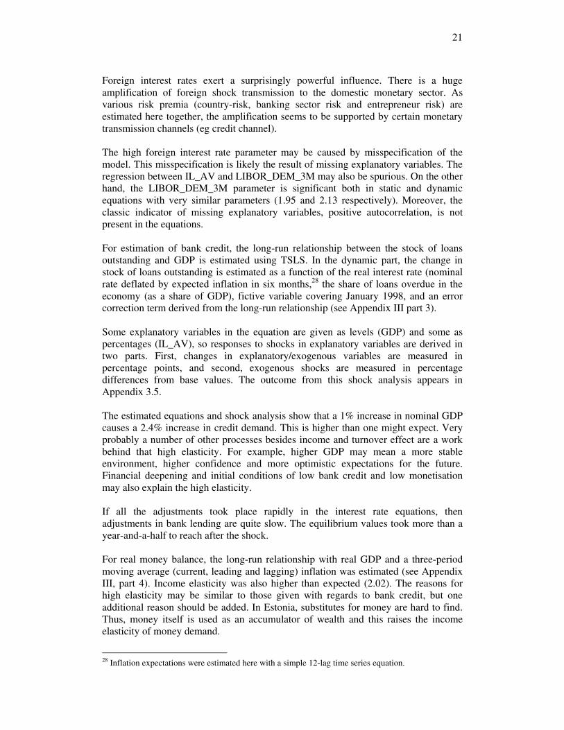
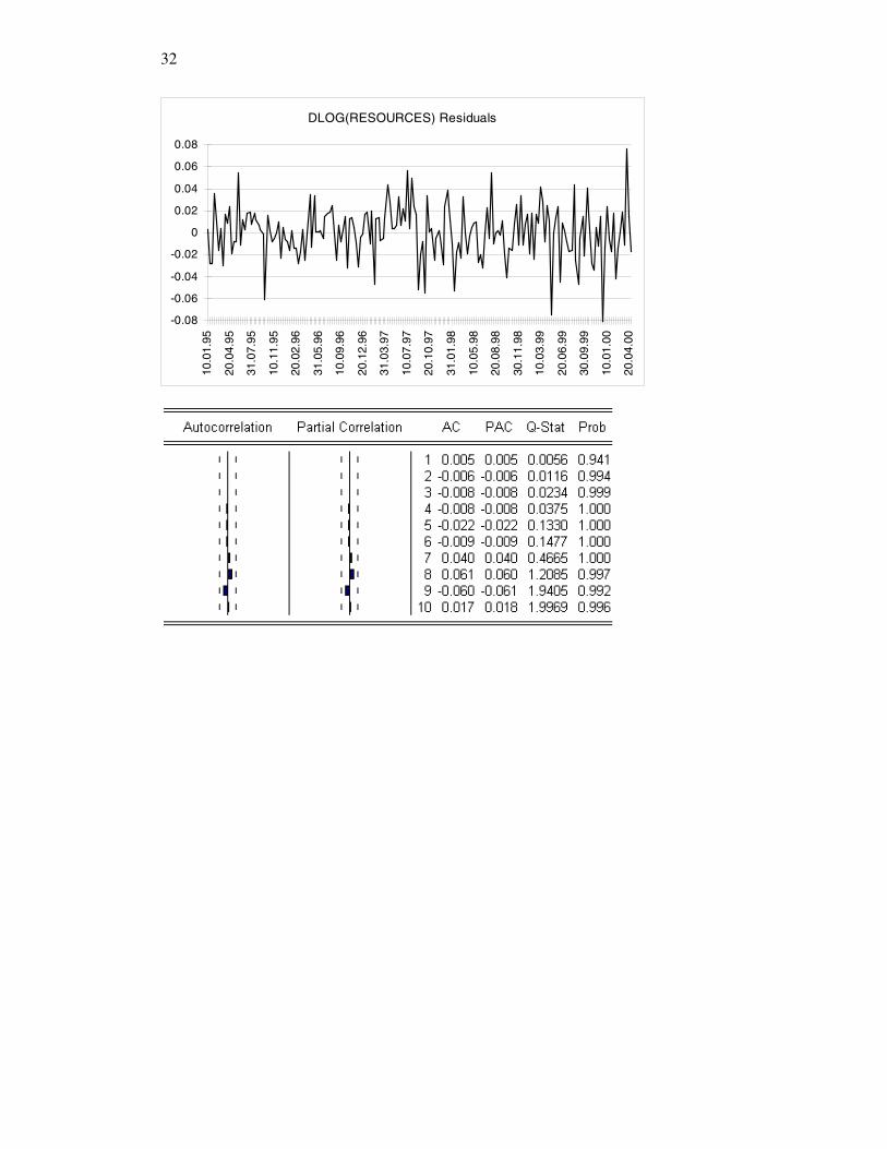
To test which model specification holds on empirical data, first causality betweencredit provided to private sector and resources of commercial banks20 was tested usingthe Granger causality test.21 As commercial banks can most likely adjust their assetsand liabilities rapidly, tests were performed on data with monthly and 10dayfrequencies.22 The test results were similar regardless of frequency, rejecting the zerohypothesis of growth in commercial bank resources being not caused by changes inbank lending (test with residuals from corresponding VARs are reported in AppendixI). A stability test of estimated VAR parameters was also performed. The resultsshowed that parameters of the function with bank resources on the left side were farmore stable over time than the parameters of the function with loans on the left side(at both monthly and 10day frequencies). In the estimated function explainingchanges in lending resources, there was a temporary shock to the parameters at theend of 1997. Eventually, the parameters return to their original path. Both of theseanalyses reject the hypothesis that there have been long-lasting (over two months)restrictions on the supply of foreign debt capital and show that causality hasconsistently run from loans to bank resources. The assumption of possible long-lasting (over a year) restrictions on the supply foreign debt capital was brought up byanalysis of domestic interest rates in section dealing with monetary sector under aCBA. We have already noted that shocks are clearly reflected in domestic moneymarket rates, but changes and possible causes of changes in lending rates are not soclear.

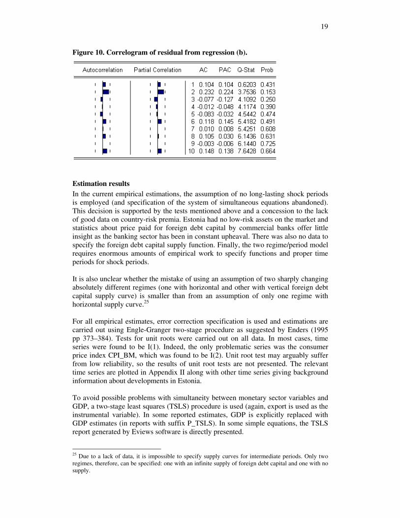
The next test determines error correction from equations for lending rate using twotime samples. The first (regression a) was estimated for the period from 1995m3 to1999m8. The second (regression b) excludes all observations between 1997m9 to1999m3 (suspect for shock). The interest rate equation was specified as function ofbase interest rate (London Interbank 3month Deutsche Mark Offer Rate), inflation,and real economic growth23 (actually a proxy estimated from real export) asfundamental variables.24 Residuals from these two regressions are plotted in Figure 8with correlograms in Figures 9 and 10. One can see that the regression excludingpossible shock period underestimates interest rates during the period excluded from

20 Credit provided to the private sector is defined as the sum of loans outstanding and the amount ofbought domestic debt securities. Commercial banks’ resources are defined as the sum of amounts owedto customers; amounts owed to foreign credit institutions; issued debt securities and share capital minusthe sum of claims on the central bank, foreign debt securities held by foreign residents and other assets.21 Appropriate lag length was derived by estimating VAR between same variables and minimizingAkaike info criterion. As there is no proper test to decide whether one VAR is significantly better thanother one with slightly different lag length, causality tests were also carried out with lag lengths closeto one with minimal Akaike info criterion and test results were very similar to the ones reported.22 Commercial banks balance sheets are reported approximately every 10 days.23 There are no official data about monthly GDP, so a simple interpolation was carried out (both forreal and nominal GDP). Quarterly GDP was first divided equally between corresponding months, thenthese series were smoothed with a three-period moving average (current, leading and lagging).24 The reasoning behind the equation is provided with empirical estimates of interest rate equation.

18

the estimates. Nevertheless, this difference is relatively small, so one might argue thattime period left out from regression b is the only period of serious economic recessionduring the sample and estimations excluding period of recession will not averageasymmetry effect over movements to the both sides. This argument is supported bythe beautifully distributed residual from regression a, which shows no signs of shockslasting longer than the shaded time period. Also there are no signs of positiveautocorrelation that might indicate a systematic error in the ex-post simulations.

Figure 8. Ex-post simulation errors from lending rate equation.

-0.02

-0.01

0.00

0.01

0.02

95:07 96:01 96:07 97:01 97:07 98:01 98:07 99:01 99:07

Residuals from regression (a) Residuals from regression (b)

Figure 9. Correlogram of residual from regression (a).

19

Figure 10. Correlogram of residual from regression (b).

Estimation resultsIn the current empirical estimations, the assumption of no long-lasting shock periodsis employed (and specification of the system of simultaneous equations abandoned).This decision is supported by the tests mentioned above and a concession to the lackof good data on country-risk premia. Estonia had no low-risk assets on the market andstatistics about price paid for foreign debt capital by commercial banks offer littleinsight as the banking sector has been in constant upheaval. There was also no data tospecify the foreign debt capital supply function. Finally, the two regime/period modelrequires enormous amounts of empirical work to specify functions and proper timeperiods for shock periods.

It is also unclear whether the mistake of using an assumption of two sharply changingabsolutely different regimes (one with horizontal and other with vertical foreign debtcapital supply curve) is smaller than from an assumption of only one regime withhorizontal supply curve.25

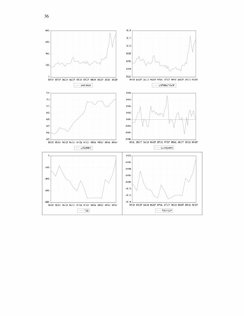
For all empirical estimates, error correction specification is used and estimations arecarried out using Engle-Granger two-stage procedure as suggested by Enders (1995pp 373–384). Tests for unit roots were carried out on all data. In most cases, timeseries were found to be I(1). Indeed, the only problematic series was the consumerprice index CPI_BM, which was found to be I(2). Unit root test may arguably sufferfrom low reliability, so the results of unit root tests are not presented. The relevanttime series are plotted in Appendix II along with other time series giving backgroundinformation about developments in Estonia.

To avoid possible problems with simultaneity between monetary sector variables andGDP, a two-stage least squares (TSLS) procedure is used (again, export is used as theinstrumental variable). In some reported estimates, GDP is explicitly replaced withGDP estimates (in reports with suffix P_TSLS). In some simple equations, the TSLSreport generated by Eviews software is directly presented.

25 Due to a lack of data, it is impossible to specify supply curves for intermediate periods. Only tworegimes, therefore, can be specified: one with an infinite supply of foreign debt capital and one with nosupply.

20

For lending rate, two equations are estimated. The first ignores changes in costs facedby commercial banks coming from Eesti Pank monetary policy exercises with reserverequirement and remuneration rate (specification 1). The second estimates directly thetotal risk premium (including country risk, banking sector risk and lender risk) againstthe average lending rate and London Interbank Offer Rate (specification 2). From thatdifference, the directly derived cost coming from reserve requirement is subtracted.26

There is the slightly problematic assumption that costs faced from reserverequirements equal to London Interbank Offer Rate. Here it seems reasonable thatsuch money is probably lent at slightly higher rates. Also there are few dynamics frommonetary policy exercises as there are only two changes in variable irr as reserverequirement and remuneration rates both changed only once (see Appendix II.Evolution of Eesti Pank monetary policy operational framework), which makes theoutcomes of both estimation approaches quite similar.

In both cases, the lending rate is specified as a function of the 3month LondonInterbank Deutsche Mark Offer Rate (LIBOR_DEM_3M), inflation (CPI_12M), andreal economic growth (RGDP_12M). LIBOR_DEM_3M presents international (base)interest rate and inflation with economic growth represents fundamental variablesaffecting risk premia asked. Problems with simultaneity also led to exclusion of thecurrent account balance (TSB/GDP). The current account balance may have an impacton risk premia asked by foreign debt capital suppliers, but lower interest rates willhave a direct negative impact on the current account balance. Preliminary testsindicated no clear relationship between domestic interest rates and the current accountbalance.

Estimation results with most primary statistics are presented in Appendix IV, parts 1and 2. Also included are plotted residuals from dynamic regression, ex-postsimulation and responses to changes in explanatory variables.27 As indicated by highvalues in the error-correction term in dynamic equations, the long-run levels afterexogenous shocks are attained within a few periods. The long-run influences(depending on equation specification) are as follows:

LIBOR_DEM_3M CPI_12M RGDP_12M R IR_REMSpecification 1 1.951 0.152 -0.122 0.000 0.000Specification 2 1.932 0.157 -0.130 0.050 -0.149

26 If we assume that the banking sector is competitive, we also must assume that the price of bankcredit equals the price of foreign liabilities plus costs related to lending business. As amounts held onrequired reserve accounts do not bear interest (or the rate is well above the market average), additionalreserve requirements are also additional costs for commercial banks. Under assumed conditions, wecan derive an equation for the price of bank credit:

δ-r

riii

r*

+⋅−=)(1

where i is price of credit form costs side, i* price of money commercial banks have to pay to foreignfinancial institutions (includes country and domestic banking sector risk premium), δ is cost related tolending activity, ir is interest paid by central bank from reserves (remunerator) and r is legal reserverequirement. If we assume that demand for bank loans is a negative function of the lending rate andthat the supply of foreign capital is elastic, then increased reserve requirements (r) will reduce bankloans outstanding and an increased remunerator (ir) will have a positive impact on lending activity.27 It is important to note that as model tested here is partial and covers only the monetary sector. Theresponse tests only describe properties of estimated equations, not absorption of shocks by theaggregate economy.

21

Foreign interest rates exert a surprisingly powerful influence. There is a hugeamplification of foreign shock transmission to the domestic monetary sector. Asvarious risk premia (country-risk, banking sector risk and entrepreneur risk) areestimated here together, the amplification seems to be supported by certain monetarytransmission channels (eg credit channel).

The high foreign interest rate parameter may be caused by misspecification of themodel. This misspecification is likely the result of missing explanatory variables. Theregression between IL_AV and LIBOR_DEM_3M may also be spurious. On the otherhand, the LIBOR_DEM_3M parameter is significant both in static and dynamicequations with very similar parameters (1.95 and 2.13 respectively). Moreover, theclassic indicator of missing explanatory variables, positive autocorrelation, is notpresent in the equations.

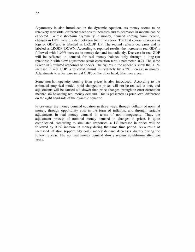
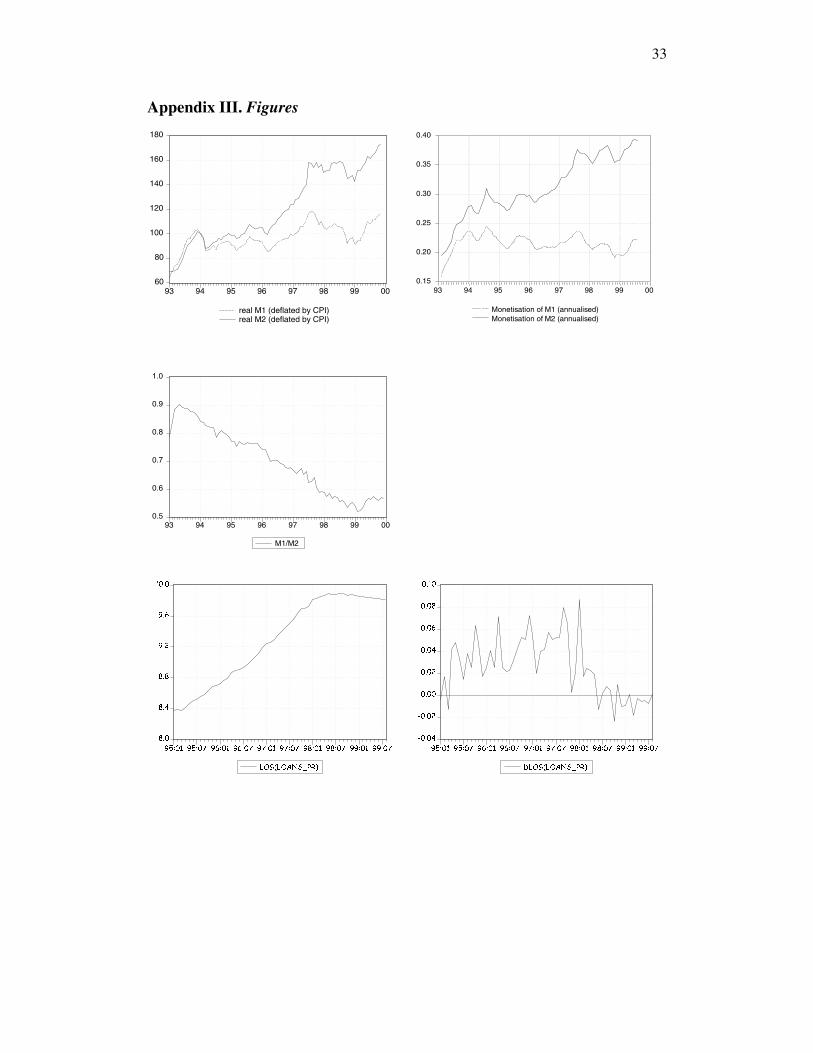
For estimation of bank credit, the long-run relationship between the stock of loansoutstanding and GDP is estimated using TSLS. In the dynamic part, the change instock of loans outstanding is estimated as a function of the real interest rate (nominalrate deflated by expected inflation in six months,28 the share of loans overdue in theeconomy (as a share of GDP), fictive variable covering January 1998, and an errorcorrection term derived from the long-run relationship (see Appendix III part 3).

Some explanatory variables in the equation are given as levels (GDP) and some aspercentages (IL_AV), so responses to shocks in explanatory variables are derived intwo parts. First, changes in explanatory/exogenous variables are measured inpercentage points, and second, exogenous shocks are measured in percentagedifferences from base values. The outcome from this shock analysis appears inAppendix 3.5.

The estimated equations and shock analysis show that a 1% increase in nominal GDPcauses a 2.4% increase in credit demand. This is higher than one might expect. Veryprobably a number of other processes besides income and turnover effect are a workbehind that high elasticity. For example, higher GDP may mean a more stableenvironment, higher confidence and more optimistic expectations for the future.Financial deepening and initial conditions of low bank credit and low monetisationmay also explain the high elasticity.

If all the adjustments took place rapidly in the interest rate equations, thenadjustments in bank lending are quite slow. The equilibrium values took more than ayear-and-a-half to reach after the shock.

For real money balance, the long-run relationship with real GDP and a three-periodmoving average (current, leading and lagging) inflation was estimated (see AppendixIII, part 4). Income elasticity was also higher than expected (2.02). The reasons forhigh elasticity may be similar to those given with regards to bank credit, but oneadditional reason should be added. In Estonia, substitutes for money are hard to find.Thus, money itself is used as an accumulator of wealth and this raises the incomeelasticity of money demand.

28 Inflation expectations were estimated here with a simple 12-lag time series equation.

22

Asymmetry is also introduced in the dynamic equation. As money seems to berelatively inflexible, different reactions to increases and to decreases in income can beexpected. To test short-run asymmetry in money, demand coming from income,changes in GDP were divided between two time series. The first covers increases inlogs of GDP and is labelled as LRGDP_UP. The second reflects decreases and islabeled as LRGDP_DOWN. According to reported results, the increase in real GDP isfollowed with 1.96% increase in money demand immediately. Decrease in real GDPwill be reflected in demand for real money balance only through a long-runrelationship with slow adjustment (error correction term’s parameter -0.2). The sameis seen in simulated responses to shocks. The figures in the appendix show that a 1%increase in real GDP is followed almost immediately by a 2% increase in money.Adjustments to a decrease in real GDP, on the other hand, take over a year.

Some non-homogeneity coming from prices is also introduced. According to theestimated empirical model, rapid changes in prices will not be realised at once andadjustments will be carried out slower than price changes through an error correctionmechanism balancing real money demand. This is presented as price level differenceon the right hand side of the dynamic equation.

Prices enter the money demand equation in three ways: through deflator of nominalmoney, through opportunity cost in the form of inflation, and through variableadjustments in real money demand in terms of non-homogeneity. Thus, theadjustment process of nominal money demand to changes in prices is quitecomplicated. According to simulated responses, a 1% increase in prices will befollowed by 0.6% increase in money during the same time period. As a result ofincreased inflation (opportunity cost), money demand decreases slightly during thefollowing year. The nominal money demand slowly regains equilibrium after twoyears.

23

5. Concluding remarks

Two alternative hypotheses about relationships in the monetary sector can beproposed. First, we can assume a close-to-perfect world and a currency boardarrangement with reliable peg. Prices in the monetary sector are set according to costsand amounts by demand at given prices. The alternative hypothesis is that close-to-perfect conditions apply most of the time, but there are also periods of seriousdisturbances in the supply of foreign capital. As we are unable to distinguish theextent to which changes in commercial banks’ liabilities are restricted by the supplyof foreign capital and by changes in demand, these alternative hypotheses are difficultto test. Thus, a visual inspection of domestic interest rates was made and two testswere performed. Figures showed that at the end of 1997, following the crisis on theTallinn Stock Exchange, some domestic interest rates increased sharply (overnightand deposit rates) while for some rates shocks were less pronounced (eg lendingrates). As a more quantitative test, the causality between bank credit to private sectorand resources of commercial banks was also tested. Tests were carried out on datawith one-month and 10day frequencies. Both test results suggested that it is morelikely that causality runs from bank credit to bank resources rather than the reverse.For the second test, an equation for lending rate was estimated and behaviour ofresiduals was inspected over the possible shock period and tested for signs of positiveautocorrelation. Positive autocorrelation would indicate that during shock periodscertain important explanatory variables are missing. Moreover, the missing part isvery likely related to constraints on supply. It turned out that residuals behaved overthe suspected shock period rather well and all changes in lending rate could beexplained with base rate and fundamentals (reflecting a part of risk premia).

According to the test results, a model for the Estonian monetary sector was developedand estimated from the demand side only. Behavioural equations were estimated fordomestic lending rates, loans provided to private sector and money demand. Thelending rate was estimated dependent on the foreign base rate and fundamentalsreflecting domestic risk premium with no impact from demand variables makingspecification consistent with assumed infinite foreign capital supply function. Forempirical estimations, specification of error correction model was employed.Estimation results were complemented with ex-post forecasts and figures presentingresponses from changes in explanatory variables over time.

The current monthly model found surprisingly high income (GDP used here as proxyfor income) elasticities of money demand and bank credit. Also impacts coming frominternational interest rates were larger than expected. The high income elasticity maybe explained by other processes that accompany the increase in GDP. These hiddenprocesses can be increased confidence, optimistic expectations about the future,higher accumulated wealth, quite possibly financial deepening etc. At the same time,model users must beware of the possibility that this elasticities may decline in thefuture.

Looking ahead, we plan to modify this model of the monetary sector to fit quarterlydata. It will be inserted into Eesti Pank’s quarterly aggregated macromodel of the

24

Estonian economy. This macromodel is used for forecast exercises (currently bankcredit is determined as exogenous variable) and hopefully will be modified soon tosuit simulation exercises as well. Additionally, equations for money multiplier will beused in estimating changes in reserves.

25

Glossary

Theoretical model specifications

δ cost margin related to lending activityπ opportunity costf banking sector’s cash (liquidity) preference ratioF vector of fundamental variablesi domestic interest ratei* foreign interest rateir required reserve’s remuneratorir real interest rateL lendingLR commercial banks resourcesM money stockP price levelr required reserve requirement ratioY output, GDPφ vector of variables reflecting information about loan portfolio

qualityγ vector of variables reflecting opportunity cost from holding

moneyσ vector of variables reflecting confidence and certainty

Empirical estimations

CPI_12M 12month inflation [CPI_12M = CPI_BM/CPI_BM(-12)-1]CPI_12MF(6) 12month inflation expectations for 6 monthsCPI_BM price level, base indexGDP gross domestic productGDPP_TSLS estimated proxy for GDP using exportID_AV average deposit rateIL_AV average lending rateIR_REM required reserve’s remuneratorLIBOR_DEM_3M from 3month London Interbank Deutsche Mark Offer RateLOANS_PR amount of banking loans provided to private sectorM2 money stock M2OVERDUE amount of loans with repayment arrearsR reserve requirement ratioREG_U registered unemploymentRGDP gross domestic product on real valuesRGDP_12M 12month growth rate for real GDP [RGDP_12M =

RGDP_BM/RGDP_BM(-12)-1]

RGDP_12MP_TSLS estimated proxy for RGDP 12month growth rates using realexports

RGDPP_TSLS estimated proxy for RGDP using real exportsRM2 real money stock M2 (RM2 = M2/CPI_BM)U unemployment (according to ILO standards)

26

Mathematical functions

LOG(x) natural logarithm of variable xD(x) first difference of variable xDLOG(x) first difference from natural logarithm of variable x@MOVAV(x,n) n period moving average of variable x

27

Appendix I. Evolution of Eesti Pank monetary policy operational framework29

Table 1 Evolution of Eesti Pank monetary policy operational framework

29 Eesti Pank 1999b, p 50

28

Table 1 (continued)

29

Appendix II. Results from Granger Causality Test and VAR regressions

Causality test using monthly dataPairwise Granger Causality Tests Sample: Jan. 1995 to Apr. 2000 Lags: 3

Null Hypothesis: Obs F-Statistic Probability

DLOG(RESOURCES) does not Granger Cause DLOG(LOANS_PR+ASSETS_01_RES)

62 0.87679 0.45881

DLOG(LOANS_PR+ASSETS_01_RES) does not Granger Cause DLOG(RESOURCES)

5.65263 0.00189

Residuals from corresponding VAR(3)

DLOG(LOANS_PR+ASSETS_01_RES) Residuals

-0.08

-0.06

-0.04

-0.02

0

0.02

0.04

0.06

0.08

31.0

1.95

30.0

4.95

31.0

7.95

31.1

0.95

31.0

1.96

30.0

4.96

31.0

7.96

31.1

0.96

31.0

1.97

30.0

4.97

31.0

7.97

31.1

0.97

31.0

1.98

30.0

4.98

31.0

7.98

31.1

0.98

31.0

1.99

30.0

4.99

31.0

7.99

31.1

0.99

31.0

1.00

30

DLOG(RESOURCES) Residuals

-0.08

-0.06

-0.04

-0.02

0

0.02

0.04

0.06

0.08

31.0

1.95

30.0

4.95

31.0

7.95

31.1

0.95

31.0

1.96

30.0

4.96

31.0

7.96

31.1

0.96

31.0

1.97

30.0

4.97

31.0

7.97

31.1

0.97

31.0

1.98

30.0

4.98

31.0

7.98

31.1

0.98

31.0

1.99

30.0

4.99

31.0

7.99

31.1

0.99

31.0

1.00

31

Causality test Using 10 day dataPairwise Granger Causality Tests Sample: 10 Jan. 1995 to 30 Apr. 2000 Lags: 9

Null Hypothesis: Obs F-Statistic Probability

DLOG(RESOURCES) does not Granger Cause DLOG(LOANS_PR+ASSETS_01_RES)

192 1.65831 0.10247

DLOG(LOANS_PR+ASSETS_01_RES) does not Granger Cause DLOG(RESOURCES)

2.22086 0.02282

Residuals from corresponding VAR(9)

DLOG(LOANS_PR+ASSETS_01_RES) Residuals

-0.08

-0.06

-0.04

-0.02

0

0.02

0.04

0.06

0.08

10.0

1.95

20.0

4.95

31.0

7.95

10.1

1.95

20.0

2.96

31.0

5.96

10.0

9.96

20.1

2.96

31.0

3.97

10.0

7.97

20.1

0.97

31.0

1.98

10.0

5.98

20.0

8.98

30.1

1.98

10.0

3.99

20.0

6.99

30.0

9.99

10.0

1.00

20.0

4.00

32

DLOG(RESOURCES) Residuals

-0.08

-0.06

-0.04

-0.02

0

0.02

0.04

0.06

0.08

10.0

1.95

20.0

4.95

31.0

7.95

10.1

1.95

20.0

2.96

31.0

5.96

10.0

9.96

20.1

2.96

31.0

3.97

10.0

7.97

20.1

0.97

31.0

1.98

10.0

5.98

20.0

8.98

30.1

1.98

10.0

3.99

20.0

6.99

30.0

9.99

10.0

1.00

20.0

4.00

33

Appendix III. Figures

60

80

100

120

140

160

180

93 94 95 96 97 98 99 00

real M1 (deflated by CPI)real M2 (deflated by CPI)

0.15

0.20

0.25

0.30

0.35

0.40

93 94 95 96 97 98 99 00

Monetisation of M1 (annualised)Monetisation of M2 (annualised)

0.5

0.6

0.7

0.8

0.9

1.0

93 94 95 96 97 98 99 00

M1/M2

8.0

8.4

8.8

9.2

9.6

10.0

95:01 95:07 96:01 96:07 97:01 97:07 98:01 98:07 99:01 99:07

LOG(LOANS_PR)

-0.04

-0.02

0.00

0.02

0.04

0.06

0.08

0.10

95:01 95:07 96:01 96:07 97:01 97:07 98:01 98:07 99:01 99:07

DLOG(LOANS_PR)

34

8.10

8.15

8.20

8.25

8.30

8.35

95:01 95:07 96:01 96:07 97:01 97:07 98:01 98:07 99:01 99:07

LOG(RGDP)

-0.02

-0.01

0.00

0.01

0.02

95:01 95:07 96:01 96:07 97:01 97:07 98:01 98:07 99:01 99:07

DLOG(RGDP)

0.00

0.02

0.04

0.06

0.08

0.10

0.12

0.14

93 94 95 96 97 98 99 00

REG_U REG_U_SA U

0.010

0.015

0.020

0.025

0.030

0.035

0.040

93 94 95 96 97 98 99 00

REG_U_SA REG_U

-0.10

-0.05

0.00

0.05

0.10

0.15

95:01 95:07 96:01 96:07 97:01 97:07 98:01 98:07 99:01 99:07

RGDP_12M

-0.03

-0.02

-0.01

0.00

0.01

0.02

0.03

95:01 95:07 96:01 96:07 97:01 97:07 98:01 98:07 99:01 99:07

D(RGDP_12M)

7.8

8.0

8.2

8.4

8.6

8.8

95:01 95:07 96:01 96:07 97:01 97:07 98:01 98:07 99:01 99:07

LOG(GDP)

-0.01

0.00

0.01

0.02

0.03

0.04

95:01 95:07 96:01 96:07 97:01 97:07 98:01 98:07 99:01 99:07

DLOG(GDP)

35

4.6

4.7

4.8

4.9

5.0

5.1

5.2

95:01 95:07 96:01 96:07 97:01 97:07 98:01 98:07 99:01 99:07

LOG(CPI_BM)

-0.01

0.00

0.01

0.02

0.03

0.04

95:01 95:07 96:01 96:07 97:01 97:07 98:01 98:07 99:01 99:07

DLOG(CPI_BM)

0.0

0.1

0.2

0.3

0.4

95:01 95:07 96:01 96:07 97:01 97:07 98:01 98:07 99:01 99:07

CPI_12M

-0.10

-0.08

-0.06

-0.04

-0.02

0.00

0.02

0.04

95:01 95:07 96:01 96:07 97:01 97:07 98:01 98:07 99:01 99:07

D(CPI_12M)

0.025

0.030

0.035

0.040

0.045

0.050

0.055

95:01 95:07 96:01 96:07 97:01 97:07 98:01 98:07 99:01 99:07

LIBOR_DEM_3M

-0.004

-0.002

0.000

0.002

0.004

95:01 95:07 96:01 96:07 97:01 97:07 98:01 98:07 99:01 99:07

D(LIBOR_DEM_3M)

0.08

0.10

0.12

0.14

0.16

0.18

0.20

0.22

95:01 95:07 96:01 96:07 97:01 97:07 98:01 98:07 99:01 99:07

IL_AV

-0.03

-0.02

-0.01

0.00

0.01

0.02

0.03

95:01 95:07 96:01 96:07 97:01 97:07 98:01 98:07 99:01 99:07

D(IL_AV)

36

0

200

400

600

800

95:01 95:07 96:01 96:07 97:01 97:07 98:01 98:07 99:01 99:07

OVERDUE

0.02

0.04

0.06

0.08

0.10

0.12

0.14

95:01 95:07 96:01 96:07 97:01 97:07 98:01 98:07 99:01 99:07

OVERDUE/GDP

4.5

4.6

4.7

4.8

4.9

5.0

5.1

5.2

95:01 95:07 96:01 96:07 97:01 97:07 98:01 98:07 99:01 99:07

LOG(RM2)

-0.06

-0.04

-0.02

0.00

0.02

0.04

0.06

0.08

95:01 95:07 96:01 96:07 97:01 97:07 98:01 98:07 99:01 99:07

DLOG(RM2)

-800

-600

-400

-200

0

95:01 95:07 96:01 96:07 97:01 97:07 98:01 98:07 99:01 99:07

TSB

-0.14

-0.12

-0.10

-0.08

-0.06

-0.04

-0.02

0.00

95:01 95:07 96:01 96:07 97:01 97:07 98:01 98:07 99:01 99:07

TSB/GDP

37

Appendix IV. Statistical protocols1. Statistical protocols for lending rate equation (without costs from reserves)

1.1. Johansen test for cointegrationSample: Mar 1995 to Aug 1999 Included observations: 54 Test assumption: No deterministic trend in the data Series: IL_AV LIBOR_DEM_3M CPI_12M RGDP_12MP_TSLS Lags interval: 1 to 1

Likelihood 5 Percent 1 Percent Hypothesised Eigenvalue Ratio Critical Value Critical Value No. of CE(s)

0.478724 59.32361 53.12 60.16 None * 0.223497 24.14393 34.91 41.07 At most 1 0.142235 10.48438 19.96 24.60 At most 2 0.039911 2.199403 9.24 12.97 At most 3

*(**) denotes rejection of the hypothesis at 5% (1%) significance level L.R. test indicates 1 cointegrating equation(s) at 5% significance level Normalised Cointegrating Coefficients: 1 Cointegrating Equation(s)

IL_AV LIBOR_DEM_3M CPI_12M RGDP_12MP_TSLS C 1.000000 -1.704298 -0.166623 0.178427 -0.064704

(0.17647) (0.01090) (0.02137) (0.00517)

1.2. Long-run relationshipDependent Variable: IL_AV Method: Least Squares Sample: 1995:03 1999:08 Included observations: 54

Variable Coefficient Std. Error t-Statistic Prob.

LIBOR_DEM_3M 1.951061 0.212686 9.173417 0.0000 CPI_12M 0.151774 0.012952 11.71867 0.0000

RGDP_12MP_TSLS -0.122031 0.019556 -6.240224 0.0000 C 0.053387 0.006285 8.494333 0.0000

R-squared 0.94001 Mean dependent var 0.14082 Adjusted R-squared 0.93641 S.D. dependent var 0.02403 S.E. of regression 0.00606 Akaike info criterion -7.30278 Sum squared resid 0.00183 Schwarz criterion -7.15545 Log likelihood 201.175 F-statistic 261.180 Durbin-Watson stat 1.87671 Prob(F-statistic) 0.00000

1.3. Error-correction modelDependent Variable: D(IL_AV) Method: Least Squares Sample: 1995:04 1999:08 Included observations: 53


ECT_il_av(-1) -0.999581 0.146810 -6.808663 0.0000 D(CPI_12M) 0.182934 0.064261 2.846746 0.0064

D(RGDP_12MP_TSLS) -0.237346 0.095719 -2.479614 0.0166 D(LIBOR_DEM_3M) 2.129417 0.706248 3.015112 0.0041

R-squared 0.56455 Mean dependent var -0.00162 Adjusted R-squared 0.53789 S.D. dependent var 0.00877 S.E. of regression 0.00595 Akaike info criterion -7.33524 Sum squared resid 0.00174 Schwarz criterion -7.18654 Log likelihood 198.383 Durbin-Watson stat 2.00303

38

1.4. Residuals from error-correction model and ex-post simulation results

-0.02

-0.01

0.00

0.01

0.02

-0.03

-0.02

-0.01

0.00

0.01

0.02

95:07 96:01 96:07 97:01 97:07 98:01 98:07 99:01 99:07

Residual Actual Fitted

-0.02

-0.01

0.00

0.01

0.02

0.08

0.10

0.12

0.14

0.16

0.18

0.20

95:07 96:01 96:07 97:01 97:07 98:01 98:07 99:01 99:07

Residual IL_AV IL_AVF

39

1.5. Simulated responses (in pp) to 1 pp permanent innovation in independentvariables (shock moment 01:2000)

0.00

0.05

0.10

0.15

0.20

1999 2000 2001 2002 2003 2004 2005

innovation in CPI_12M

-0.25

-0.20

-0.15

-0.10

-0.05

0.00

1999 2000 2001 2002 2003 2004 2005

innovation in RGDP_12M

-1.0

-0.5

0.0

0.5

1.0

1999 2000 2001 2002 2003 2004 2005

innovation in IR_REM

-1.0

-0.5

0.0

0.5

1.0

1999 2000 2001 2002 2003 2004 2005

innovation in R

0.0

0.5

1.0

1.5

2.0

2.5

1999 2000 2001 2002 2003 2004 2005

innovation in LIBOR_DEM_3M

2. Statistical protocols for lending rate equation (using costs from reserves)

2.1. Johansen test for cointegrationSample: Mar 1995 to Aug 1999 Included observations: 54 Test assumption: No deterministic trend in the data Series: IL_AV-(LIBOR_DEM_3M-IR_REM*R)/(1-R) CPI_12M RGDP_12MP_TSLS LIBOR_DEM_3M Lags interval: 1 to 1

Likelihood 5 Percent 1 Percent Hypothesized Eigenvalue Ratio Critical Value Critical Value No. of CE(s)

0.516856 62.46058 53.12 60.16 None ** 0.218081 23.17880 34.91 41.07 At most 1 0.131309 9.894613 19.96 24.60 At most 2 0.041576 2.293124 9.24 12.97 At most 3

*(**) denotes rejection of the hypothesis at 5% (1%) significance level L.R. test indicates 1 cointegrating equation(s) at 5% significance level

Normalised Cointegrating Coefficients: 1 Cointegrating Equation(s)

IL_AV- (LIBOR_DEM_3M-IR_REM*R) /(1-R)

CPI_12M RGDP_12MP_TSLS LIBOR_DEM_3M C

1.000000 -0.170710 0.180881 -0.550725 -0.065338 (0.01020) (0.02034) (0.16557) (0.00485)

40

2.2. Long-run relationshipDependent Variable: IL_AV-(LIBOR_DEM_3M-IR_REM*R)/(1-R) Method: Least Squares Sample: 1995:03 1999:08 Included observations: 54


CPI_12M 0.156919 0.013170 11.91525 0.0000 RGDP_12MP_TSLS -0.130328 0.019885 -6.554156 0.0000

C 0.054917 0.006391 8.593089 0.0000 LIBOR_DEM_3M 0.782160 0.216268 3.616623 0.0007


2.3. Error-correction modelDependent Variable: D(IL_AV-(LIBOR_DEM_3M-IR_REM*R)/(1-R)) Method: Least Squares Sample: Apr 1995 to Aug 1999 Included observations: 53


ECT_il_av(-1) -1.072484 0.144932 -7.399934 0.0000 D(CPI_12M) 0.215619 0.065268 3.303619 0.0018

D(RGDP_12MP_TSLS) -0.190008 0.094196 -2.017147 0.0491

R-squared 0.53579 Mean dependent var -0.00107 Adjusted R-squared 0.51722 S.D. dependent var 0.00874 S.E. of regression 0.00608 Akaike info criterion -7.31421 Sum squared resid 0.00185 Schwarz criterion -7.20269 Log likelihood 196.827 Durbin-Watson stat 1.89791


-0.02

-0.01

0.00

0.01

0.02

-0.03

-0.02

-0.01

0.00

0.01

0.02

95:07 96:01 96:07 97:01 97:07 98:01 98:07 99:01 99:07


41

-0.02

-0.01

0.00

0.01

0.02

0.08

0.10

0.12

0.14

0.16

0.18

0.20

95:07 96:01 96:07 97:01 97:07 98:01 98:07 99:01 99:07

IL_AV-IL_AVF IL_AV IL_AVF

2.5. Simulated responses (in pp) to 1 pp permanent innovation in independentvariables (shock moment 01:2000)

0.00

0.05

0.10

0.15

0.20

0.25

1999 2000 2001 2002 2003 2004 2005

innovation in CPI_12M

-0.20

-0.15

-0.10

-0.05

0.00

1999 2000 2001 2002 2003 2004 2005

innovation in RGDP_12M

-0.16

-0.12

-0.08

-0.04

0.00

1999 2000 2001 2002 2003 2004 2005

innovation in IR_REM

0.00

0.01

0.02

0.03

0.04

0.05

0.06

1999 2000 2001 2002 2003 2004 2005

innovation in R

0.0

0.5

1.0

1.5

2.0

2.5

1999 2000 2001 2002 2003 2004 2005

innovation in LIBOR_DEM_3M

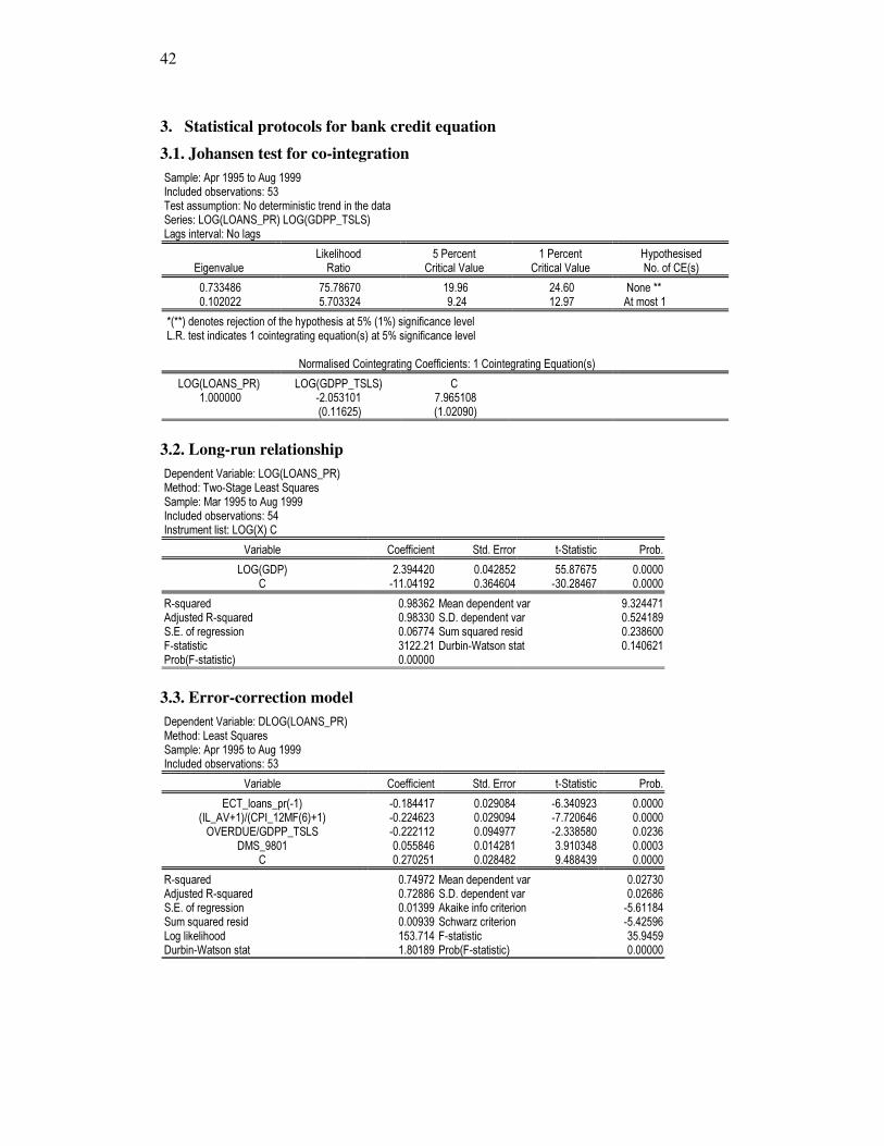
42

3. Statistical protocols for bank credit equation

3.1. Johansen test for co-integrationSample: Apr 1995 to Aug 1999 Included observations: 53 Test assumption: No deterministic trend in the data Series: LOG(LOANS_PR) LOG(GDPP_TSLS) Lags interval: No lags


0.733486 75.78670 19.96 24.60 None ** 0.102022 5.703324 9.24 12.97 At most 1



LOG(LOANS_PR) LOG(GDPP_TSLS) C 1.000000 -2.053101 7.965108

(0.11625) (1.02090)

3.2. Long-run relationshipDependent Variable: LOG(LOANS_PR) Method: Two-Stage Least Squares Sample: Mar 1995 to Aug 1999 Included observations: 54 Instrument list: LOG(X) C


LOG(GDP) 2.394420 0.042852 55.87675 0.0000 C -11.04192 0.364604 -30.28467 0.0000

R-squared 0.98362 Mean dependent var 9.324471 Adjusted R-squared 0.98330 S.D. dependent var 0.524189 S.E. of regression 0.06774 Sum squared resid 0.238600 F-statistic 3122.21 Durbin-Watson stat 0.140621 Prob(F-statistic) 0.00000

3.3. Error-correction modelDependent Variable: DLOG(LOANS_PR) Method: Least Squares Sample: Apr 1995 to Aug 1999 Included observations: 53


ECT_loans_pr(-1) -0.184417 0.029084 -6.340923 0.0000 (IL_AV+1)/(CPI_12MF(6)+1) -0.224623 0.029094 -7.720646 0.0000

OVERDUE/GDPP_TSLS -0.222112 0.094977 -2.338580 0.0236 DMS_9801 0.055846 0.014281 3.910348 0.0003

C 0.270251 0.028482 9.488439 0.0000


43


-0.04

-0.02

0.00

0.02

0.04

-0.05

0.00

0.05

0.10

95:07 96:01 96:07 97:01 97:07 98:01 98:07 99:01 99:07


-0.06

-0.04

-0.02

0.00

0.02

0.04

0.06

0

5000

10000

15000

20000

25000

95:07 96:01 96:07 97:01 97:07 98:01 98:07 99:01 99:07

Residual (%) LOANS_PR LOANS_PRF

44

3.5. Simulated responses (in %) to 1% / 1 pp permanent innovation inindependent variables (shock moment 01:2000)

-0.08

-0.06

-0.04

-0.02

0.00

1999 2000 2001 2002 2003 2004 2005

1% innovation in OVERDUE

0.0

0.5

1.0

1.5

2.0

2.5

3.0

1999 2000 2001 2002 2003 2004 2005

1 % innovation in GDP

-1.2

-1.0

-0.8

-0.6

-0.4

-0.2

0.0

1999 2000 2001 2002 2003 2004 2005

1 pp. innovation in IL_AV

0.0

0.2

0.4

0.6

0.8

1.0

1.2

1.4

1999 2000 2001 2002 2003 2004 2005

1 pp. innovation in CPI_12M6

4. Statistical protocols for real money demand equation

4.1. Johansen test for cointegrationSample: Mar 1995 to Aug 1999 Included observations: 54 Test assumption: No deterministic trend in the data Series: LOG(RM2) LOG(RGDP) @MOVAV(CPI_12M(1),3) Lags interval: No lags


0.486283 47.81774 34.91 41.07 None ** 0.141412 11.84928 19.96 24.60 At most 1 0.064773 3.616137 9.24 12.97 At most 2



LOG(RM2) LOG(RGDP) @MOVAV(CPI_12M(1),3) C 1.000000 -1.008819 1.033102 3.177488

(0.62820) (0.41797) (5.26369)

45

4.2. Long-run relationshipDependent Variable: LOG(RM2) Method: Least Squares Sample(adjusted): Apr 1995 to Nov 1999 Included observations: 56 after adjusting endpoints


LOG(RGDP) 2.022336 0.110420 18.31494 0.0000 @MOVAV(CPI_12M(1),3) -0.483480 0.087057 -5.553629 0.0000

C -11.68384 0.920825 -12.68844 0.0000


4.3. Error-correction modelDependent Variable: DLOG(RM2) Method: Least Squares Sample: Mar 1995 to Aug 1999 Included observations: 54


ECT_m2(-1) -0.209706 0.069634 -3.011558 0.0041 DLOG(CPI_BM) -0.366105 0.162252 -2.256405 0.0286

LRGDP_UP 1.963785 0.315525 6.223864 0.0000 DMS_9707 0.047940 0.013702 3.498732 0.0010 DMS_9708 0.042820 0.013582 3.152699 0.0028 DMS_9810 -0.041540 0.013237 -3.138241 0.0029

R-squared 0.64232 Mean dependent var 0.00951 Adjusted R-squared 0.60506 S.D. dependent var 0.02105 S.E. of regression 0.01323 Akaike info criterion -5.70804 Sum squared resid 0.00840 Schwarz criterion -5.48704 Log likelihood 160.117 Durbin-Watson stat 1.29890


-0.04

-0.02

0.00

0.02

0.04

-0.05

0.00

0.05

0.10

95:07 96:01 96:07 97:01 97:07 98:01 98:07 99:01 99:07


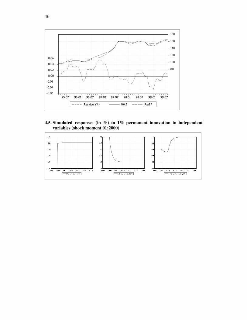
46

-0.06

-0.04

-0.02

0.00

0.02

0.04

0.06

80

100

120

140

160

180

95:07 96:01 96:07 97:01 97:07 98:01 98:07 99:01 99:07

Residual (%) RM2 RM2F

4.5. Simulated responses (in %) to 1% permanent innovation in independentvariables (shock moment 01:2000)

0.0

0.5

1.0

1.5

2.0

2.5

1999 2000 2001 2002 2003 2004 2005

1 % increase in RGDP

-2.5

-2.0

-1.5

-1.0

-0.5

0.0

1999 2000 2001 2002 2003 2004 2005

1 % decrease in RGDP

0.0

0.2

0.4

0.6

0.8

1.0

1999 2000 2001 2002 2003 2004 2005

1 % innovation in CPI_BM

47

References

Bernanke, Ben S. and Gertler, Mark (1995), Inside the Black Box: The Credit Channelof Monetary Policy Transmission, The Journal of Economic Perspectives, 9, Fall

Catao, Luis (1997), Bank Credit in Argentina in the Aftermath of the Mexican Crisis:Supply or Demand Constrained?, IMF Working Paper No WP/97/32

Eesti Pank (1996), Eesti Pank Bulletin, No 1, 1996

Eesti Pank (1998), Eesti Pank Bulletin, No 5 (40), 1998(also accessible from http://www.ee/epbe/en/publication.html)

Eesti Pank (1999a), Eesti Pank 1919–1999, Tallinn, 1999

Eesti Pank (1999b), Eesti Pank Annual Report 1998(also accessible from http://www.ee/epbe/1999/eng/)

Eesti Pank (1999c), Eesti Pank Bulletin, No 1 (43), 1999

Enders, Walter (1995), Applied Econometric Time Series. John Wiley & Sons, Inc

Engle, F. R., Granger, C. W. J. (1987) Co-Integration and Error Correction:Representation, Estimation and Testing, Econometrica 55: pp 251–276

Fase, M.M.G. (1995), The demand for commercial bank loans and the lending rate,European Economic Review 39, pp 99–115

Fase, Martin M.G. (1999), On Interest Rates and Asset Prices in Europe. The selectedEssays of Martin M. G. Fase, Edward Elgar Publishing Limited, UK

Korhonen, Iikka (1999), Currency Boards in the Baltic Countries: What Have WeLearned?, BOFIT Discussion Papers No 6/999

Laidler, David. E. W. (1993) The Demand for Money: Theories, Evidence andProblems. 4th ed New York: HarperCollins College Publishers

Lepik, Ilmar (1999), Basic Features of the Estonian Currency Board: Convertibility andLiquidity Management, Prepared for the International Workshop on CurrencyBoards, Hong Kong Baptist University, October 1999

Lättemäe, Raoul and Randveer, Martti (2000), Currency boards versus flexibleexchange rate regimes, Global And International Tendencies in the Banking Sector,Warsaw, National Bank of Poland, April 2000, pp 36–40

Mishkin, Frederic S. (1996), The Channels of Monetary Transmission: Lessons forMonetary Policy, NBER Working Paper Series, Working Paper No 5464

48

Niggle, Christopher J. (1991), The Endogenous Money Supply Theory: AnInstitutionalist Appraisal, Journal of Economic Issues, Vol. XXV, No 1 March, pp137–51

Olexa, Michal (1998), Analysis and Econometric Modelling of the Monetary Sector inthe Slovak Republic, Institute for Advanced Studies, Transition Economies SeriesNo 1

Rother, Philipp (1999), Explaining the Behavior of Financial Intermediation – Evidencefrom Transition Economies, IMF Working Paper No WP/99/36

Sepp, Urmas, Pikkani, Rasmus and Rell, Mari (1999), Eesti majanduse makromudel.Lühitutvustus, Eesti Panga Toimetised nr 2, 1999

Sepp, Urmas (1999), Factors of Trade-Deficit Convergence in Estonia, Working Papersof Eesti Pank No 1, 1999

Sriram, Subramanian (1999), Survey of Literature on Demand for Money: Theoreticaland Empirical Work with Special, IMF Working Paper WP/99/64

The Monetary Sector under a Currency Board Arrangement ... · The Monetary Sector under a Currency...

Documents

Transcript of The Monetary Sector under a Currency Board Arrangement ... · The Monetary Sector under a Currency...