The Modeling Power of the Periodic Event Scheduling...
38
The Modeling Power of the Periodic Event Scheduling Problem: Railway Timetables — and Beyond Christian Liebchen and Rolf H. M¨ ohring TU Berlin, Institut f¨ ur Mathematik, Straße des 17. Juni 136, D-10623 Berlin {liebchen,moehring}@math.tu-berlin.de Abstract. In the planning process of railway companies, we propose to integrate important decisions of network planning, line planning, and vehicle scheduling into the task of periodic timetabling. From such an integration, we expect to achieve an additional potential for optimization. Models for periodic timetabling are commonly based on the Periodic Event Scheduling Problem (PESP). We show that, for our purpose of this integration, the PESP has to be extended by only two features, namely a linear objective function and a symmetry requirement. These extensions of the PESP do not really impose new types of constraints. Indeed, prac- titioners have already required them even when only planning timetables autonomously without interaction with other planning steps. Even more important, we only suggest extensions that can be formulated by mixed integer linear programs. Moreover, in a selfcontained presentation we summarize the tradi- tional PESP modeling capabilities for railway timetabling. For the first time, also special practical requirements are considered that we proove not being expressible in terms of the PESP. 1 Introduction Traditionally, the planning process of railway companies is subdivided into sev- eral tasks. From the strategic level down to the operational level, the most promi- nent subtasks are network planning, line planning, timetable generation, vehicle scheduling, crew scheduling, and crew rostering, see Figure 1. For a detailed description of these planning steps, as well as for an overview of solution approaches, we refer to Bussieck, Winter, and Zimmermann [4]. Notice that network planning and line planning are of course part of the strategic plan- ning process of public transportation companies. In contrast, vehicle scheduling and crew scheduling are of operational nature. In between, timetabling forms the linkage between service and operation. An important reason for the divi- sion into at least five subtasks is the high complexity of the overall planning process ([4], [7]). Supported by the DFG Research Center “Mathematics for key technologies” in Berlin. F. Geraets et al. (Eds.): Railway Optimization 2004, LNCS 4359, pp. 3–40, 2007. c Springer-Verlag Berlin Heidelberg 2007
Transcript of The Modeling Power of the Periodic Event Scheduling...
The Modeling Power of thePeriodic Event Scheduling Problem:Railway Timetables — and Beyond�
Christian Liebchen and Rolf H. Mohring
TU Berlin, Institut fur Mathematik, Straße des 17. Juni 136, D-10623 Berlin{liebchen,moehring}@math.tu-berlin.de
Abstract. In the planning process of railway companies, we proposeto integrate important decisions of network planning, line planning, andvehicle scheduling into the task of periodic timetabling. From such anintegration, we expect to achieve an additional potential for optimization.
Models for periodic timetabling are commonly based on the PeriodicEvent Scheduling Problem (PESP). We show that, for our purpose of thisintegration, the PESP has to be extended by only two features, namely alinear objective function and a symmetry requirement. These extensionsof the PESP do not really impose new types of constraints. Indeed, prac-titioners have already required them even when only planning timetablesautonomously without interaction with other planning steps. Even moreimportant, we only suggest extensions that can be formulated by mixedinteger linear programs.
Moreover, in a selfcontained presentation we summarize the tradi-tional PESP modeling capabilities for railway timetabling. For the firsttime, also special practical requirements are considered that we proovenot being expressible in terms of the PESP.
1 Introduction
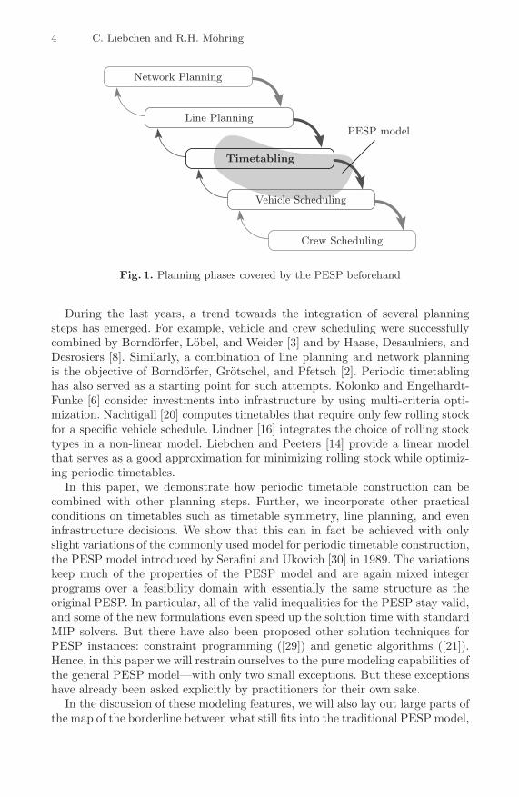
Traditionally, the planning process of railway companies is subdivided into sev-eral tasks. From the strategic level down to the operational level, the most promi-nent subtasks are network planning, line planning, timetable generation, vehiclescheduling, crew scheduling, and crew rostering, see Figure 1.
For a detailed description of these planning steps, as well as for an overview ofsolution approaches, we refer to Bussieck, Winter, and Zimmermann [4]. Noticethat network planning and line planning are of course part of the strategic plan-ning process of public transportation companies. In contrast, vehicle schedulingand crew scheduling are of operational nature. In between, timetabling formsthe linkage between service and operation. An important reason for the divi-sion into at least five subtasks is the high complexity of the overall planningprocess ([4], [7]).
� Supported by the DFG Research Center “Mathematics for key technologies”in Berlin.
F. Geraets et al. (Eds.): Railway Optimization 2004, LNCS 4359, pp. 3–40, 2007.c© Springer-Verlag Berlin Heidelberg 2007
4 C. Liebchen and R.H. Mohring
Network Planning
Line Planning
Timetabling
Vehicle Scheduling
Crew Scheduling
PESP model
Fig. 1. Planning phases covered by the PESP beforehand
During the last years, a trend towards the integration of several planningsteps has emerged. For example, vehicle and crew scheduling were successfullycombined by Borndorfer, Lobel, and Weider [3] and by Haase, Desaulniers, andDesrosiers [8]. Similarly, a combination of line planning and network planningis the objective of Borndorfer, Grotschel, and Pfetsch [2]. Periodic timetablinghas also served as a starting point for such attempts. Kolonko and Engelhardt-Funke [6] consider investments into infrastructure by using multi-criteria opti-mization. Nachtigall [20] computes timetables that require only few rolling stockfor a specific vehicle schedule. Lindner [16] integrates the choice of rolling stocktypes in a non-linear model. Liebchen and Peeters [14] provide a linear modelthat serves as a good approximation for minimizing rolling stock while optimiz-ing periodic timetables.
In this paper, we demonstrate how periodic timetable construction can becombined with other planning steps. Further, we incorporate other practicalconditions on timetables such as timetable symmetry, line planning, and eveninfrastructure decisions. We show that this can in fact be achieved with onlyslight variations of the commonly used model for periodic timetable construction,the PESP model introduced by Serafini and Ukovich [30] in 1989. The variationskeep much of the properties of the PESP model and are again mixed integerprograms over a feasibility domain with essentially the same structure as theoriginal PESP. In particular, all of the valid inequalities for the PESP stay valid,and some of the new formulations even speed up the solution time with standardMIP solvers. But there have also been proposed other solution techniques forPESP instances: constraint programming ([29]) and genetic algorithms ([21]).Hence, in this paper we will restrain ourselves to the pure modeling capabilities ofthe general PESP model—with only two small exceptions. But these exceptionshave already been asked explicitly by practitioners for their own sake.
In the discussion of these modeling features, we will also lay out large parts ofthe map of the borderline between what still fits into the traditional PESP model,
The Modeling Power of the PESP: Railway Timetables — and Beyond 5
and what requires new features, and at which cost. To this end, we also review thetraditional PESP modeling issues, thus altogether providing a selfcontained pre-sentation of the PESP modeling capabilities and its extensions to symmetry, lineplanning, and network planning. Any of our suggestions for integrating these fea-tures can be formulated as a MIP, in particular not involving any quadratic terms.
The paper is organized as follows. Section 2 introduces the PESP. It presentsits main formulations as a graph theoretic potential problem and as a mixedinteger program, and reports on its complexity and a useful characterization ofperiodic timetables.
Section 3 discusses requirements for cyclic timetables that can be met by thePESP. These include simple requirements such as collision-free traffic on singletracks and headway between successive trains, but also more sophisticated onessuch as bundling of lines, train coupling and sharing, fixed events in connectionwith hierarchical planning, and also disjunctive constraints and soft constraints.
Section 4 is devoted to timetable requirements that are beyond the scope ofthe traditional PESP, such as balanced reduction of service and symmetry oftimetables. We show that the PESP or its MIP model only needs to be extendedslightly in order to accommodate symmetry requirements.
Finally, in Section 5, we consider the integration of aspects of other planningsteps into periodic timetable construction, in particular vehicle scheduling (min-imization of rolling stock), line planning (simultaneous construction of line planand timetable), and network planning (making infrastructure decisions). Thisintegration makes essential use of the flexibility of the PESP, in particular dis-junctive constraints, uses symmetry and, as a new technique, integrates aspectsof graph techniques into the PESP in order to handle line planning.
All model features are illustrated by examples from our practical experiencewith timetable construction at Deutsche Bahn AG, S-Bahn Berlin GmbH, andBVG (Berlin Underground).
2 The Periodic Event Scheduling Problem (PESP)
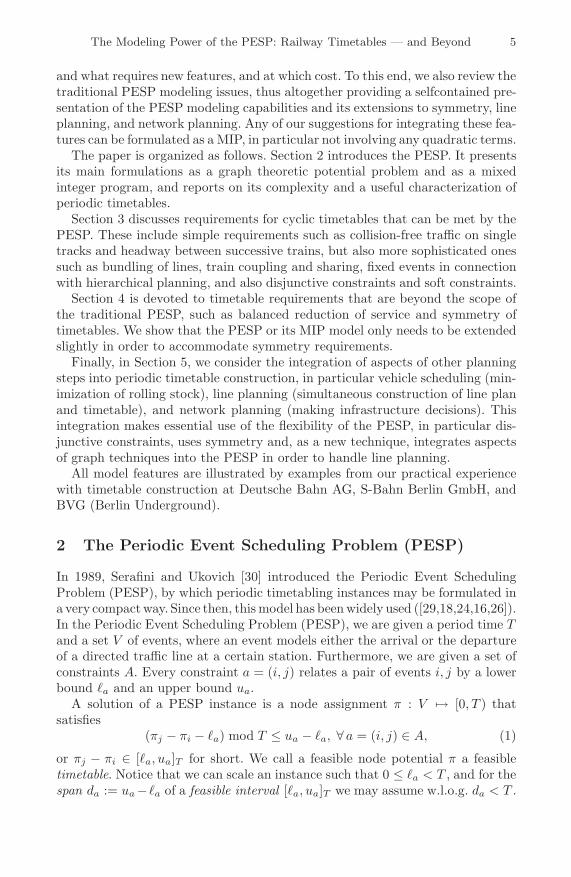
In 1989, Serafini and Ukovich [30] introduced the Periodic Event SchedulingProblem (PESP), by which periodic timetabling instances may be formulated ina very compactway. Since then, this model has been widely used ([29,18,24,16,26]).In the Periodic Event Scheduling Problem (PESP), we are given a period time Tand a set V of events, where an event models either the arrival or the departureof a directed traffic line at a certain station. Furthermore, we are given a set ofconstraints A. Every constraint a = (i, j) relates a pair of events i, j by a lowerbound �a and an upper bound ua.
A solution of a PESP instance is a node assignment π : V �→ [0, T ) thatsatisfies
(πj − πi − �a) mod T ≤ ua − �a, ∀ a = (i, j) ∈ A, (1)
or πj − πi ∈ [�a, ua]T for short. We call a feasible node potential π a feasibletimetable. Notice that we can scale an instance such that 0 ≤ �a < T , and for thespan da := ua − �a of a feasible interval [�a, ua]T we may assume w.l.o.g. da < T .
6 C. Liebchen and R.H. Mohring
Furthermore, for every fixed event i0, every fixed point of time t0 ∈ [0, T ), andevery feasible timetable π there exists an equivalent timetable π′ with π′
i0= t0.
This is achieved by performing the simple shift π′i := (πi −(πi0 − t0)) mod T . Let
us denote by D = (V, A, �, u) the constraint graph modeling a PESP instance.There are several practical aspects of periodic timetabling which profit from
the presence of a linear objective function of the form∑
a=(i,j)∈A
wa · (πj − πi − �a) mod T,
with weights wa. In our opinion, the most striking one is the integration of centralaspects of vehicle scheduling, cf. section 5.1.
Another perspective on periodic scheduling can be obtained by consideringtensions instead of potentials. In a straightforward way, define for a given nodepotential π its tension
xa := πj − πi, ∀a = (i, j) ∈ A.
We call a set of edges C ⊆ A an oriented cycle if re-orienting a subset of itsedges yields a directed circuit. The incidence vector γC of an oriented cycle Cis a vector in {−1, 0, 1}A, where the entry minus one indicates a backward arcof the oriented cycle. The cycle space C of a directed graph D is defined as
C := span{γC | C oriented cycle in D}.
Recall that a vector x is a tension (or potential difference), if and only iffor some cycle basis B of C, and each of its oriented cycles C ∈ B with inci-dence vectors γC it holds that γC x = 0 (e.g. [1]). This yields the following MIPformulation
min ct(x + pT )s.t. Γ x = 0
� ≤ x + pT ≤ up ∈ Z
A,
or
min ctxs.t. Γ (x − pT ) = 0
� ≤ x ≤ up ∈ Z
A,
⎤
⎥⎥⎦ (2)
where Γ ∈ {−1, 0, 1}(|A|−|V |+1)×|A| denotes the cycle-arc incidence matrix (cyclematrix ) of some cycle basis of the directed graph D. The x variables are in facta periodic tension, which we formally define for a given node potential π to be
xij := (πj − πi − �ij) mod T + �ij .
Sometimes, it is useful to define slack variables xa := xa − �a.Recall that cycle matrices are totally unimodular ([28]). This is the main
observation to prove the following lemma.
Lemma 1 ([23]). Let I denote an instance of PESP with integral vectors � andu and an integer period time T . If I admits some feasible timetable π ∈ [0, T )V ,then it also admits an integral feasible timetable π′ ∈ {0, . . . , T − 1}V .
Already Serafini and Ukovich made the following simple but useful observation.
The Modeling Power of the PESP: Railway Timetables — and Beyond 7
Lemma 2 (Serafini and Ukovich [30]). If we relax the requirement π ∈[0, T )V to π ∈ Q
V , then for every spanning tree H and every feasible timetable πthere exists an equivalent feasible timetable π′ which induces pa = 0 for a ∈ H.
Notice that we may interpret the remaining non-zero integer variables as therepresentants of the elements of a (strictly) fundamental cycle basis. A gener-alization to integral cycle bases yields many variants of problem formulation 2,some of which are easier to solve for MIP solvers ([12]).
Periodic tensions can be characterized similarly to classic aperiodic tensions.
Lemma 3 (Cycle Periodicity Property). A vector x ∈ QA is a periodic
tension, if and only if for every cycle C with incidence vector γC ∈ {−1, 0, 1}A,there exists some zC ∈ Z, such that
γCx = zCT. (3)
The PESP is NP-complete, since it generalizes Vertex Coloring ([23]). To seethis, orient the edges of a Coloring instance arbitrarily and assign feasible peri-odic intervals [1, T −1]T to each of them. Solution methods for the PESP includeConstraint Programming ([29]), Genetic Algorithms ([21]), and of course integerprogramming techniques. For a computational study in that these substantiallydifferent approaches are compared to each other, we refer to [15]. For the MIPapproach, a very important ingredient is
Theorem 1 (Odijk [24]). An integer vector p allows a feasible solution for theMIP (2), if and only if for every oriented cycle C of the constraint graph, thefollowing cycle inequalities hold
pC
:=
⎡
⎢⎢⎢1T
(∑
a∈C+
�a −∑
a∈C−ua)
⎤
⎥⎥⎥≤
∑
a∈C+
pa −∑
a∈C−pa ≤
⎢⎢⎢⎣ 1T
(∑
a∈C+
ua −∑
a∈C−�a)
⎥⎥⎥⎦ =: pC , (4)
where C+ and C− denote the forward and the backward arcs of the cycle C.
We close this section by listing other totally different practical applications whichcan be modeled via the PESP ([30]). The most prominent ones are the schedulingof systems of traffic lights, and periodic job shop scheduling.
3 Timetabling Requirements Covered by the PESP
This section gives a broad overview of the timetable modeling capabilities of thePESP. Contrary to the following sections, practical requirements to be modeledare limited to those arising in periodic timetabling. Nevertheless, there are manyfacts we have to discuss in order to give a self-contained overview.
However, let us start by naming two facts which are definitely beyond thescope of the PESP: routing of trains through stations or even alternative tracks,and routing of the passenger flow. Hence, throughout this paper we assume fixedroutes for both trains and passengers. A short motivation for these assumptionswill be given at the beginning of Section 4.
8 C. Liebchen and R.H. Mohring
KölnHbf
Köln−Deutz
WuppertalDüsseldorf
Abzw. Gummersbacher Str.
Köln−Mülheim
High−speed−track (Frankfurt)
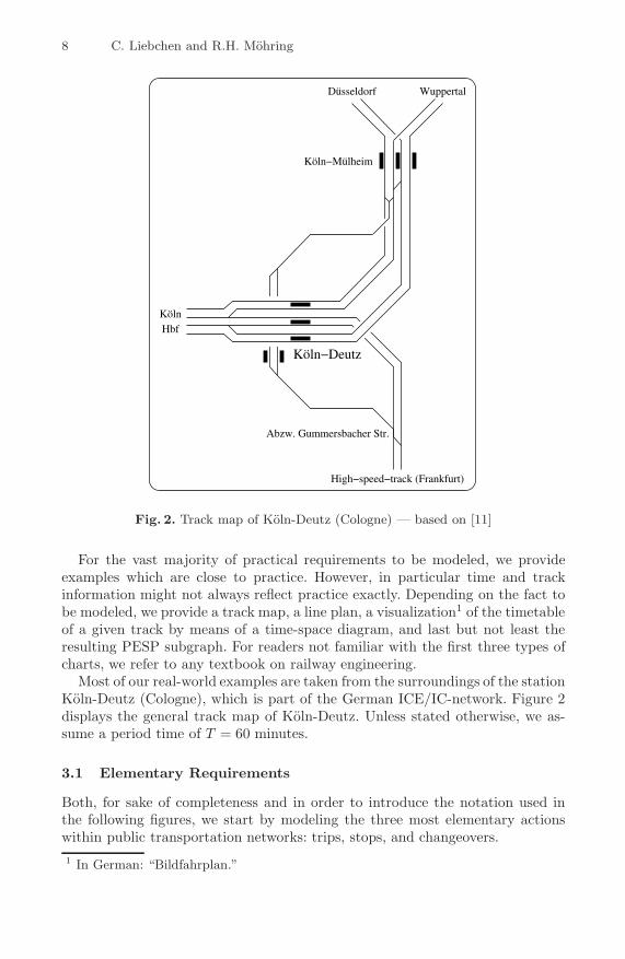
Fig. 2. Track map of Koln-Deutz (Cologne) — based on [11]
For the vast majority of practical requirements to be modeled, we provideexamples which are close to practice. However, in particular time and trackinformation might not always reflect practice exactly. Depending on the fact tobe modeled, we provide a track map, a line plan, a visualization1 of the timetableof a given track by means of a time-space diagram, and last but not least theresulting PESP subgraph. For readers not familiar with the first three types ofcharts, we refer to any textbook on railway engineering.
Most of our real-world examples are taken from the surroundings of the stationKoln-Deutz (Cologne), which is part of the German ICE/IC-network. Figure 2displays the general track map of Koln-Deutz. Unless stated otherwise, we as-sume a period time of T = 60 minutes.
3.1 Elementary Requirements
Both, for sake of completeness and in order to introduce the notation used inthe following figures, we start by modeling the three most elementary actionswithin public transportation networks: trips, stops, and changeovers.1 In German: “Bildfahrplan.”

The Modeling Power of the PESP: Railway Timetables — and Beyond 9
KölnHbf
Köln−Deutz
WuppertalDüsseldorf
Abzw. Gummersbacher Str.
Köln−Mülheim
High−speed−track (Frankfurt)
Köln−Deutz
Frankfurt
Paris
Amsterdam
Dortmund
[�a, ua], wa
[6, 65], 119
[4, 4], 0[3, 8], 266
stop arc
trip arc
changeover
Koln-Deutz
Fig. 3. Modeling elementary requirements: (a) two disjoint routes of lines serv-ing Koln-Deutz; (b) the corresponding line plan; (c) PESP constraints modeling run-ning activities, stopping activities, and changeover activities
In Figure 3 (a), we highlight the tracks used by two lines which cross atKoln-Deutz. The lines themselves are given in Figure 3 (b). Finally, we providethe constraint graph which models running, stopping, and changeover activitiesof these lines at Koln-Deutz in Figure 3 (c) as PESP constraints. For instance, the
10 C. Liebchen and R.H. Mohring
trip arc with the constraint [4, 4]60 ensures a trip time of precisely four minutesfrom Koln-Deutz to Koln Hbf. Within Koln Hbf, the minimum stopping time isset to three minutes such that passengers can board and alight the train. Finally,the increase of travel time for passengers that stay within the train is boundedby additional five minutes, providing an upper bound of 3 + 5 = 8.
Notice that we ensure changeover quality by linearly penalizing changeovertimes which exceed a certain minimal changeover time required for changingplatforms. In our example, a minimal changeover time of six minutes is assumedwhen connecting from Dortmund to Frankfurt. Using this approach, changeoverarcs typically have a wide span.
An alternative way of modeling changeovers is to require some important onesnot to exceed a maximal amount of effective waiting time. Then, we end up withrather small spans for changeover arcs. Schrijver and Steenbeek [29] follow thisapproach, which seems to be very suitable for constraint programming solvers.
Stopping arcs typically have very small span. In rather unimportant stations,in general it is a good choice to fix the span to zero, in particular if there isneither a junction of tracks, nor a single track, nor any changeovers.
Just as trip arcs, stopping arcs with span zero constitute redundancies whichcan be eliminated very efficiently in a preprocessing step. For example, one cancontract any fixed arc, i.e. having zero span, together with its target node. Doingso, the arcs which were incident with the contracted target node only have tobe redirected to the source node of the contracted arc, after having shifted theirfeasible intervals appropriately. Moreover, an arc being (anti-) parallel to anotherone can eliminated, if its feasible interval is a superset of the other arc. In additionto nodes with degree at most two, Lindner [16] gives further situations in whichthe graph can be simplified.
If there are several lines using the same track into the same direction, some-times a balanced service might be required. For n lines, this can easily be achievedby introducing arcs with feasible interval [T
n , T − Tn ]T between any unordered
pair of events that represent the departure at the first station of the commontrack. Certainly, strict balancedness may be relaxed by increasing the feasibleinterval.
Safety Requirements. If, in contrast to the previous discussion, there is noneed for a balanced service, then at least a minimal headway h between any twoof them has to be ensured. In the easiest case, the lines are operated with thesame type of trains, and their running time is fixed. Then, we can sufficientlyseparate any two lines by introducing constraints similar to the above ones,having feasible interval [h, T −h]T . These can be inserted either at the beginningor at the end of their common track. The more sophisticated constellation oftrains involving different speeds will be discussed in Section 3.2.
But two trains may also use the same track in opposite directions. This ismainly the case for single tracks, see Figure 4 (a). Obviously, a train may notenter the single track until the train of the opposite direction has left it. In Fi-gure 4 (b), we give a timetable visualization that is extremely useful in particularfor single tracks. We assume a fixed local signaling, and the grey boxes visualize

The Modeling Power of the PESP: Railway Timetables — and Beyond 11
Köln−Deutz
Abzw. Gummersbacher Str.
High−speed−track (Frankfurt)
KKDZ
Abzw. G
.
0
T}
t1
}t1
}t2
[�a, ua]
[t1, t1]
[t2, t2]
[0, T − (t1 + t2)]
Koln-Deutz (KKDZ)
Fig. 4. Modeling single tracks: (a) a single track south of Koln-Deutz; (b) visualiza-tion of a feasible timetable for that single track; (c) PESP constraints ensuring safetydistance for single track
the time a train blocks a certain part of the track. Surprisingly, there is onlyone single constraint needed to prevent two trains of opposite directions fromcolliding within the single track, as can be seen in Figure 4 (c). To that end,consider the western entry point to the single track. A train may only enter the
12 C. Liebchen and R.H. Mohring
single track after a train of the opposite direction has left (�a = 0). But it alsomust have left the single track before the next train of the opposite directionmay enter the single track (ua = T − (t1 + t2)).
Note that so far we did not care about any buffer times and blocking timeswhen setting the feasible interval to [0, T − (t1 + t2)]T . Assuming a minimalcrossing time b at both endpoints of the single track, i.e. the time that has topass from a train leaving the single track until a train in opposite direction mayenter, we obtain the following feasible interval
[b, T − (t1 + t2 + b)]T .
Again, if there are several lines that have to be scheduled on a single track, oneconstraint for every unordered pair of opposite directions is needed.
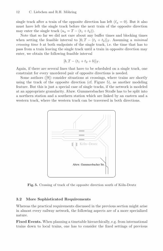
Some authors ([9]) consider situations at crossings, where trains are shortlyusing the track of the opposite direction (cf. Figure 5), as another modelingfeature. But this is just a special case of single tracks, if the network is modeledat an appropriate granularity. Abzw. Gummersbacher Straße has to be split intoa northern station and a southern station which are linked by an eastern and awestern track, where the western track can be traversed in both directions.
Köln−Deutz
Abzw. Gummersbacher Str.
Fig. 5. Crossing of track of the opposite direction south of Koln-Deutz
3.2 More Sophisticated Requirements
Whereas the practical requirements discussed in the previous section might arisein almost every railway network, the following aspects are of a more specializednature.
Fixed Events. When planning a timetable hierarchically, e.g. from internationaltrains down to local trains, one has to consider the fixed settings of previous

The Modeling Power of the PESP: Railway Timetables — and Beyond 13
hierarchies without replanning their times. Hence, the capability to fix an eventto a certain point of time is another important modeling feature.
Fortunately, due to the periodic nature of the PESP, we may shift everyfeasible timetable such that a fixed event i0 is fixed to a desired point in time t0 ∈[0, T ), i.e. πi0 = t0, and the objective value remains unchanged. By defining oneof the events to be fixed as a kind of “anchor” event, we can easily relate the otherevents ij to be fixed to certain points of time tj by introducing arcs aj = (i0, ij)with �aj = uaj = tj − t0.
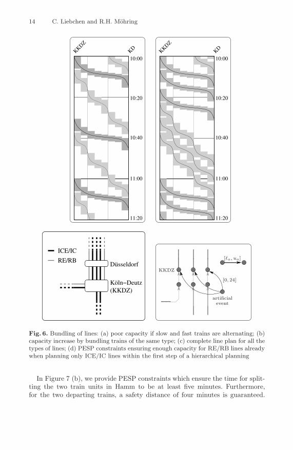
Bundling of Lines. Hierarchical planning gives rise to a further challengingaspect of timetabling. Notice that if a track is used by trains of different speeds,the capacity of that track significantly depends on the ordering of the trains.The first two parts of Figure 6 visualize this effect. In the first scenario, slowand fast trains alternate, which implies that only two hourly lines of each of thetwo train types can be scheduled. However, if lines are bundled with respect totheir speeds, three lines of the same two types of trains can be scheduled withouthaving to invest into infrastructure, cf. Figure 6 (b).
On the one hand, when only planning the high-speed lines in the first step ofa hierarchical approach, it may happen that decisions on a higher level resultin infeasibility on a lower level. On the other hand, hierarchical decompositionmight have been chosen because an overall planning was considered to be toocomplex.
In order to keep the advantage of decomposition but limit the risk of infea-sibility on lower levels, we propose to only bundle the lines of the current levelof hierarchy. Figure 6 (c) gives the complete set of lines which should be oper-ated on the track in question. In Figure 6 (d), we provide the PESP graph forthe ICE/IC network. To bundle the three active lines, we introduce an artificialevent and require each of the departure events to be sufficiently close to thatartificial event. Hereby, the departure events will be close to each other as well.
In particular, we must not choose one of the existing events as “anchor”, be-cause this would predict the corresponding line to be the head of the sequenceof bundled lines. This must definitively be avoided, because — contrary to as-sumptions made by Krista [9] — the ordering of lines is indeed a major resultof timetabling. Finally, based on profound estimates on passengers’ behaviourthe management has to decide whether it is more important to operate as manytrains as possible—and hereby bundle the trains of the same type—or whethera balanced service within the different types of trains should be preferred.
Train Coupling/Train Sharing. During the last decade, in railway passengertraffic a trend emerged towards train units which can easily be coupled andshared. Doing so, more direct connections can be offered without increasing thecapacity of some bottleneck tracks.
In Figure 7 (a), we display a line which is operated by two coupled trainunits between Berlin and Hamm. They split in Hamm to serve the two majorroutes of the Ruhr area, hereby offering direct connections from Berlin to themost important cities of that region. Still, this line occupies for example thehigh-speed track between Berlin and Hannover only once per hour.
14 C. Liebchen and R.H. Mohring
10:40
KKDZ
KD
10:00
10:20
11:00
11:20
10:40
KKDZ
KD
10:00
10:20
11:00
11:20
ICE/IC
RE/RBDüsseldorf
Köln−Deutz(KKDZ)
artificialevent
[0, 24]
[�a, ua]
KKDZ
Fig. 6. Bundling of lines: (a) poor capacity if slow and fast trains are alternating; (b)capacity increase by bundling trains of the same type; (c) complete line plan for all thetypes of lines; (d) PESP constraints ensuring enough capacity for RE/RB lines alreadywhen planning only ICE/IC lines within the first step of a hierarchical planning
In Figure 7 (b), we provide PESP constraints which ensure the time for split-ting the two train units in Hamm to be at least five minutes. Furthermore,for the two departing trains, a safety distance of four minutes is guaranteed.

The Modeling Power of the PESP: Railway Timetables — and Beyond 15
BerlinHamm
Köln−Deutz
Köln/Bonn−AirportBonn Hbf
[5, 12]
[5, 12][4, 56]
[�a, ua]
Hamm
Fig. 7. Modeling train sharing: (a) line plan for the line Berlin-Hamm-{Bonn Hbf | Koln/Bonn-Airport}; (b) PESP constraints ensuring safety distance andtime to split train units, but not specifying the ordering of departures
Notice that we do not need to specify which train should leave Hamm first.This decision will be made implicitly, and in an optimized way, by the PESPsolver.
Variable Trip Times. As long as trip times are fixed, a usual safety constraintprevents two identical trains from overtaking each other. With h being the min-imal headway for the track, we put an arc with feasible interval [h, T − h]Tbetween the two events of entering the common track. If the line at the tail ofthe constraints is by f time units faster than the line at the tail of the constraints,overtaking can be prevented by modifying the constraint to [h+ f, T −h]T . Thiscan be understood easily by having again a look at the corresponding situationin Figure 6 (a).
But this is no longer guaranteed if the model includes variable trip times. Evenensuring the minimal headway at the end of the track, too, does no longer preventovertaking (even of trains of the same type) if the span in the trip times is atleast twice the safety distance h, i.e. ua − �a ≥ 2h. Schrijver and Steenbeek [29],Lindner [16], and Kroon and Peeters [10] tackle this phenomenon by adding extraconstraints on the integer variables of the MIP formulations. Hereby, they leavethe PESP model. In addition, Kroon and Peeters [10] provide some sufficientconditions on trip times, safety distance, and on the degree of flexibility of thetrip times that prevent trains from overtaking.
16 C. Liebchen and R.H. Mohring
[r, r + h][r, r + h][r, r + h]
[r, r + h][r, r + h][r, r + h][3r, 3r + 3h]
[3r, 3r + 3h]
[h, T − h]
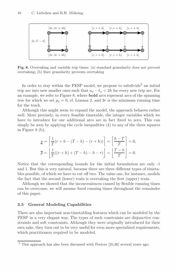
Fig. 8. Overtaking and variable trip times: (a) standard granularity does not preventovertaking; (b) finer granularity prevents overtaking
In order to stay within the PESP model, we propose to subdivide2 an initialtrip arc into new smaller ones such that ua − �a < 2h for every new trip arc. Foran example, we refer to Figure 8, where bold arcs represent arcs of the spanningtree for which we set pa = 0, cf. Lemma 2, and 3r is the minimum running timefor the track.
Although this might seem to expand the model, the approach behaves ratherwell. More precisely, in every feasible timetable, the integer variables which wehave to introduce for our additional arcs are in fact fixed to zero. This cansimply be seen by applying the cycle inequalities (4) to any of the three squaresin Figure 8 (b),
p =⌈
1T
(r + h − (T − h) − (r + h))⌉
=⌈
h − T
T
⌉= 0,
p =⌊
1T
((r + h) + (T − h) − h − r)⌋
=⌊
T − h
T
⌋= 0.
Notice that the corresponding bounds for the initial formulation are only -1and 1. But this is very natural, because there are three different types of timeta-bles possible, of which we have to cut off two. The value one, for instance, modelsthe fact that the second (lower) train is overtaking the first (upper) train.
Although we showed that the inconveniences caused by flexible running timescan be overcome, we will assume fixed running times throughout the remainderof this paper.
3.3 General Modeling Capabilities
There are also important non-timetabling features which can be modeled by thePESP in a very elegant way. The types of such constraints are disjunctive con-straints and soft constraints. Although they were originally introduced for theirown sake, they turn out to be very useful for even more specialized requirements,which practitioners required to be modeled.
2 This approach has also been discussed with Peeters [25,26] several years ago.
The Modeling Power of the PESP: Railway Timetables — and Beyond 17
[�1, u1]T
[�2, u2]T
T/0
�1
u2�2
u1
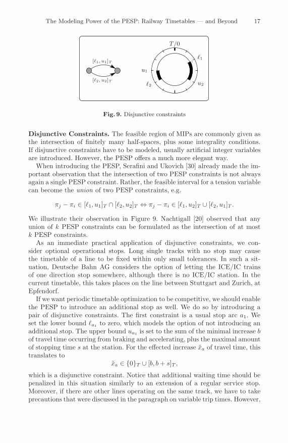
Fig. 9. Disjunctive constraints
Disjunctive Constraints. The feasible region of MIPs are commonly given asthe intersection of finitely many half-spaces, plus some integrality conditions.If disjunctive constraints have to be modeled, usually artificial integer variablesare introduced. However, the PESP offers a much more elegant way.
When introducing the PESP, Serafini and Ukovich [30] already made the im-portant observation that the intersection of two PESP constraints is not alwaysagain a single PESP constraint. Rather, the feasible interval for a tension variablecan become the union of two PESP constraints, e.g.
πj − πi ∈ [�1, u1]T ∩ [�2, u2]T ⇔ πj − πi ∈ [�1, u2]T ∪ [�2, u1]T .
We illustrate their observation in Figure 9. Nachtigall [20] observed that anyunion of k PESP constraints can be formulated as the intersection of at mostk PESP constraints.
As an immediate practical application of disjunctive constraints, we con-sider optional operational stops. Long single tracks with no stop may causethe timetable of a line to be fixed within only small tolerances. In such a sit-uation, Deutsche Bahn AG considers the option of letting the ICE/IC trainsof one direction stop somewhere, although there is no ICE/IC station. In thecurrent timetable, this takes places on the line between Stuttgart and Zurich, atEpfendorf.
If we want periodic timetable optimization to be competitive, we should enablethe PESP to introduce an additional stop as well. We do so by introducing apair of disjunctive constraints. The first constraint is a usual stop arc a1. Weset the lower bound �a1 to zero, which models the option of not introducing anadditional stop. The upper bound ua1 is set to the sum of the minimal increase bof travel time occurring from braking and accelerating, plus the maximal amountof stopping time s at the station. For the effected increase xa of travel time, thistranslates to
xa ∈ {0}T ∪ [b, b + s]T ,
which is a disjunctive constraint. Notice that additional waiting time should bepenalized in this situation similarly to an extension of a regular service stop.Moreover, if there are other lines operating on the same track, we have to takeprecautions that were discussed in the paragraph on variable trip times. However,
18 C. Liebchen and R.H. Mohring
optional operational stops make most sense within long single tracks. But there,in many cases there are not several lines using that large bottleneck.
Obviously, the introduction of an additional stop can also be due to the con-struction of a new station. Since such decisions are a part of network planning,we postpone this discussion until Section 5.3.
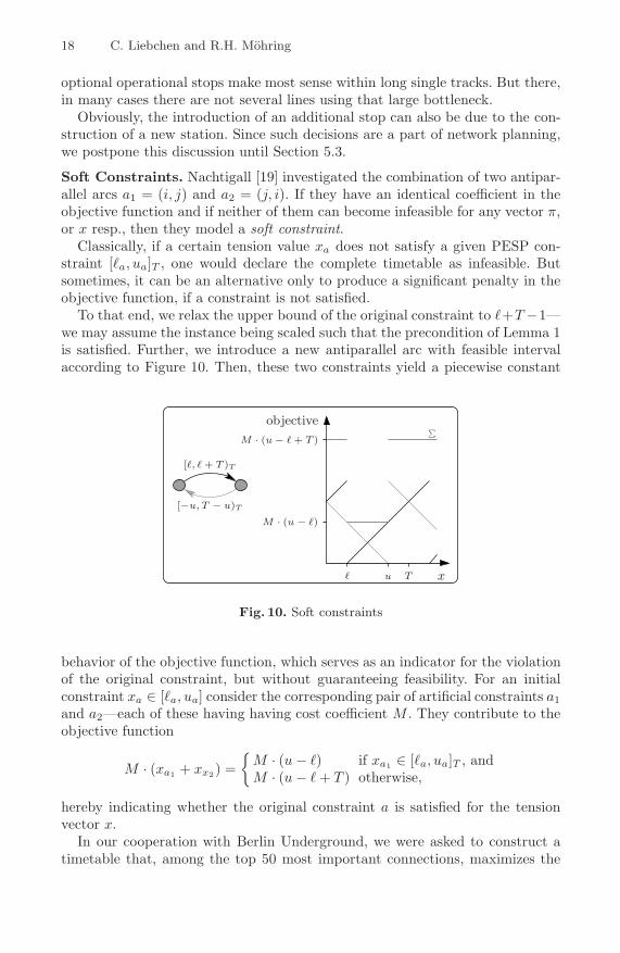
Soft Constraints. Nachtigall [19] investigated the combination of two antipar-allel arcs a1 = (i, j) and a2 = (j, i). If they have an identical coefficient in theobjective function and if neither of them can become infeasible for any vector π,or x resp., then they model a soft constraint.
Classically, if a certain tension value xa does not satisfy a given PESP con-straint [�a, ua]T , one would declare the complete timetable as infeasible. Butsometimes, it can be an alternative only to produce a significant penalty in theobjective function, if a constraint is not satisfied.
To that end, we relax the upper bound of the original constraint to �+T −1—we may assume the instance being scaled such that the precondition of Lemma 1is satisfied. Further, we introduce a new antiparallel arc with feasible intervalaccording to Figure 10. Then, these two constraints yield a piecewise constant
[�, � + T )T
[−u, T − u)T
T� u x
∑objective
M · (u − �)
M · (u − � + T )
Fig. 10. Soft constraints
behavior of the objective function, which serves as an indicator for the violationof the original constraint, but without guaranteeing feasibility. For an initialconstraint xa ∈ [�a, ua] consider the corresponding pair of artificial constraints a1and a2—each of these having having cost coefficient M . They contribute to theobjective function
M · (xa1 + xx2) ={
M · (u − �) if xa1 ∈ [�a, ua]T , andM · (u − � + T ) otherwise,
hereby indicating whether the original constraint a is satisfied for the tensionvector x.
In our cooperation with Berlin Underground, we were asked to construct atimetable that, among the top 50 most important connections, maximizes the
The Modeling Power of the PESP: Railway Timetables — and Beyond 19
number of connections having a waiting time of at most five minutes. In fact,soft constraints are well-suited for letting MIP solvers produce a timetable beingoptimal subject to this kind of objective function.
4 Timetabling Requirements Not Covered by the PESP
Although the most important practical requirements for a periodic timetablecan be modeled within the PESP, we are still aware of some special featuresfor which the PESP fails. To the best of our knowledge this is the first timethat practical requirements of timetabling are proven to be beyond the scope ofthe PESP.
First, one may think of situations in which it is not fixed which trains areoperated on which track, for example within stations. Consider a station havingtwo tracks in the same direction and three lines serving that direction. Then,we cannot decide a priori which pair of lines shall be within the station at thesame time, hence omitting the sequencing constraint between these two lines.This observation is the motivation for the DONS system to be subdivided intoCADANS, covering the timetabling step, and STATIONS, covering the routingaspect ([31]).
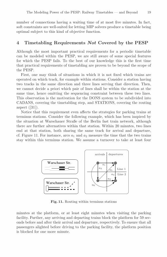
Notice that this requirement even affects the strategies for parking trains atterminus stations. Consider the following example, which has been inspired bythe situation at Warschauer Straße of the Berlin fast train network, althoughthere are further alternatives within that station. Within 20 minutes, two linesend at that station, both sharing the same track for arrival and departure,cf. Figure 11. For instance, arcs a1 and a2 measure the time that the two trainsstay within this terminus station. We assume a turnover to take at least four
Warschauer Str.
Warschauer Str.
Line 1
Line 2
arrivals departures
a1
a2
a3
a4
a5
a6
Fig. 11. Routing within terminus stations
minutes at the platform, or at least eight minutes when visiting the parkingfacility. Further, any arriving and departing trains block the platform for 59 sec-onds before and after their arrival and departure, respectively. To ensure that allpassengers alighted before driving to the parking facility, the platform positionis blocked for one more minute.

20 C. Liebchen and R.H. Mohring
Proposition 1. For every set of PESP constraints either timetables which areoperable are classified as infeasible, or timetables which are not operable areclassified as feasible.
Proof. We start by analyzing the two major strategies individually: both linesturn at the platform, or line 2 turns in the parking facility, w.l.o.g. Table 1provides tight lower and upper bounds for the six arcs in Figure 11 (c) withrespect to these two scenarios. More precisely, with a strategy specified, we havethat for every arc a = (i, j) and every value ta ∈ [ua, �a] there exists an operable
Table 1. Tight interval bounds for different turning strategies at Warschauer Straße
Arc Both at platform Line 2 to parking not specified�a ua �a ua �a ua
a1 4 12 4 13 4 13a2 4 12 8 18 4 18a3 6 14 6 17 6 17a4 6 14 2 14 2 14a5 10 18 7 18 7 18a6 10 18 6 18 6 18
timetable π such that
(πj − πi − �a) mod T = ta − �a.
Further, by simple case inspection one can verify that every operable timetablewhich implements that specific strategy respects each of the given bounds. Hence,in order to provide general PESP constraints which characterize the operabletimetables without having specified any parking strategy a priori, the feasibleintervals must include the feasible intervals of both scenarios.
However, there exists a vector π which respects the six PESP constraintsthus obtained (see the last two columns of Table 1), but which does not encodean operable timetable, because the two trains would be at the platform at thesame time: line 1 arrives at minute 00 and departs only at minute 13, althoughline 2 already arrives at minute 06 and departs at minute 16. But for each ofthe
(42
)potential differences between these four events there also exist operable
timetables that attain the very same tension value. � Hence we cannot establish a set of PESP constraints that precisely identifiespractically operable timetables as feasible solutions.
Apart from the rather important routing requirement, which unfortunatelyis simply out of scope for the PESP, we will analyze a very special situation inmore detail, namely the balanced reduction of service. Finally, we will introducethe important notion of symmetry. On the one hand, symmetry slightly exceedsthe original PESP, but on the other hand, when added explicitly, gives rise toa mechanism to include important aspects of line planning into the very sameplanning step as periodic timetabling and vehicle scheduling.

The Modeling Power of the PESP: Railway Timetables — and Beyond 21
4.1 Balanced Reduction of Service
The Berlin fast train company (S-Bahn Berlin GmbH) aims at operating onlyone timetable for one whole day. The late evening service differs from the rushhour only in that some trains are omitted. Hence, the timetable must respect theavailable capacity during the rush hour, and it has to offer a balanced service inthe late evening as well.
From a pure operations point of view, it could seem strange to sidestep anintraday change of the timetable structure. It is for sure that the informationtechnology available in the 21st century could cope with this. But it is still thepolicy of the company. It is given as a motivation that customers really expectto have only one single timetable to be kept in mind for their station.
Consider the approximately 10 km long track from Zoo station to Berlin Eaststation. On it, a minimal headway of 2.5 minutes has to be respected. The periodtime is 20 minutes and eight3 lines (having identical train types) per period anddirection have to be scheduled. In the late evening service, there are four trainsevery 20 minutes, two of them being fixed to a 10 minutes time lag. We callthese two lines core-lines.
Of course it would be ideal to have a five minutes time lag between twoconsecutive trains in the evening. But this is impossible because one of theevening trains is required to serve Potsdam every 10 minutes together with arush hour train. Hence, one should ensure that the maximal time lag betweentwo consecutive trains does not exceed 7.5 minutes.
But this simple requirement cannot be covered by the PESP. Consider the twotypes of timetables given in Table 2. Timetables of type 1 satisfy our requirement
Table 2. Possible timetables for the late evening service from Zoo station to BerlinEast station. This table only shows the core-lines that are actually running in theevenings. Each of the – entries is a joker for a rush-hour train.
Timetable Departure times (T = 20 minutes)Type 1 0.0 – – 7.5 10.0 12.5 – – (20.0)Type 2 0.0 2.5 – 7.5 10.0 – – – (20.0)
by bounding the maximum distance between two consecutive trains to 7.5 min-utes, but type 2 does not because there we have a gap of 10 minutes.
Proposition 2. For every set of PESP constraints either timetables of bothtypes are feasible, or timetables of both types are infeasible.
Proof. There are two types of constraints to be analyzed:
i. one constraint between the two non-core lines,ii. four constraints between one of the two core lines and one of the two non-core
lines.3 One of them only serves as a free slot for occasional non-passenger trips.

22 C. Liebchen and R.H. Mohring
Since we must not specify the sequence of the lines in advance, only symmetricconstraints [�, T − �]T make sense. Moreover, all constraints of type (ii) have tobe identical for the same reason.
To guarantee feasibility of type 1 timetables, we deduce � ≤ 5 for the con-straint of type (i) and � ≤ 2.5 for the constraints of type (ii). But then, timetablesof type 2 stay feasible as well. Hence, in order to cut off timetables of type 2, wehave to increment one of the given bounds. But since they are tight, this wouldimmediately cut off timetables of type 1 as well. �
Notice, however, that other railway companies implement other strategies toattain a balanced reduction of service. We will present an approach which turnsout to be easier for timetabling, but slightly more complex for operation andcustomers.
Consider the track Niederhochststadt-Langen (Hessen) via Frankfurt Hbf ofS-Bahn Frankfurt. Compare the regular service hourly pattern to the weak-trafficservice hourly pattern, which are given in Table 3. For the weak-traffic service,
Table 3. Timetables for regular service and weak-traffic service between Niederhochst-stadt and Langen (Hessen)[17]
regular service weak trafficLine S4 S3 S4 S3 S4 S3Bad Soden – 20 – 50 – 50Kronberg 09 – 39 – 24 –Niederhochststadt 14 29 44 59 29 59Langen (Hessen) 56 11 26 41 11 41Darmstadt Hbf – 25 – 55 – 55
every second train is omitted. To prevent a 45 minutes gap every hour, one ofthe two lines is shifted by 15 minutes and uses the slot of the train of the otherline, which has just been skipped.
If we assume none of the lines to share a track with other lines outside theircommon part, then we can easily deduce a feasible timetable for the weak-trafficservice from a periodic timetable, which is feasible for the regular service. In caseof single tracks along the peripherical segments, the only thing to be ensuredis that the shift of 15 minutes appears simultaneously for the two directions.Hereby, every meeting point for the weak-traffic service is already a meetingpoint for the regular service — hence, single tracks stay respected. Trivially,along the common track no conflicts will appear either.
4.2 Symmetry of a Periodic Timetable
Throughout our discussion of symmetry, we assume that for every directed linethere exists another directed line serving the same stations just in opposite order.Moreover, the concept of symmetry makes only sense, if for every traffic line,the running and stopping times of its two opposite directions are the same. Also

The Modeling Power of the PESP: Railway Timetables — and Beyond 23
for the minimum headways and other operational constraints we require themto be identical in both directions. Furthermore, the passenger flow is assumedto be symmetric.
First, observe that in every periodic timetable with period time T , every trainmeets some train of the opposite direction of its line twice within the period time.In general, every line can have different times for these meetings.
A periodic railway timetable is called symmetric with (global) axis s, if attime s every train in the network meets a train of the opposite direction of its line.From the above considerations we deduce that we may assume w.l.o.g s ∈ [0, T
2 ).For the arrival or departure event of a directed line at a certain station,
we denote by its complementary event the departure or arrival, resp., of theopposite line at the same station. In the sequel, we provide two characterizationsof symmetric timetables.
Lemma 4. A timetable is symmetric with axis s, if and only if for every pair iand i of complementary events there holds
(πi + πi) mod T
2= s. (5)
Proof. Let i and i be any two complementary events. By definition, they arepart of the two opposite directions of the same line. Moreover, they are locatedin the same station S.
In a symmetric timetable, the trains of the two opposite directions meet attimes s and s + T
2 . Consider two virtual events j and j of passing the meetingpoint M . As the trains meet there, we have πj = πj ∈ {s, s + T
2 }.We assumed the travel times of two opposite trains to be identical and denote
the travel time between S and M by t. Hence, w.l.o.g.
(πi + πi) mod T = ((πj + t) + (πj − t)) mod T = (2 · πj) mod T. �
To define a counterpart of condition (5) for the tension formulations (2), wedefine two arcs a = (i, j) and a = (j, i) to be complementary, if {i, i} and {j, j}are complementary, and we have �a = �a and ua = ua. With these definitions athand, we are able to define a symmetric instance of PESP: A constraint graphis called symmetric, if every arc connects either two complementary events, or iffor every arc a ∈ A there exists some complementary arc a ∈ A \ {a}.
Lemma 5. Consider an instance of PESP that is modeled by a connected sym-metric constraint graph. Let π be a feasible timetable with corresponding periodictension x. There exists some s ∈ [0, T
2 ) such that Condition (5) holds for everypair of symmetric events, if and only if every pair of complementary arcs a and afulfills
xa = xa. (6)

24 C. Liebchen and R.H. Mohring
Proof. “⇒”: Let a = (i, j) and a = (j, i) denote two complementary arcs of theconstraint graph. Then, we have
xa = xa − �a(2)= (πj − πi − �a) mod T
(5)= (2s − πj − (2s − πi) − �a) mod T
= (πi − πj − �a) mod T = xa − �a = xa.
“⇐”: Let x be the periodic tension of some feasible timetable π. We showthat there exists one global symmetry axis s such that Condition (5) is satisfiedfor π.
We compute s from an arbitrary fixed event, say i,
s :=(πi + πi) mod T
2.
Now, we consider an arbitrary pair of complementary events j and j. Since Dis connected and symmetric, there exists a path P from i to j or j that onlycontains arcs a such that a ∈ A \ {a}. We assume w.l.o.g. that P starts at i andends at j. By setting
xP :=∑
a∈P+
xa −∑
a∈P −
xa,
we obtain πj = (πi +xP ) mod T . As for every a ∈ P there exists its complemen-tary arc a ∈ A \ {a}, the complementary path P of P from j to i is well-defined.Equation (6) ensures xP = xP .
In total, we obtain
(πj + πj) mod T
2=
(πi + xP + πi − xP ) mod T
2=
(πi + πi) mod T
2= s. �
Remark 1. If the line plan of a traffic network is connected and the constraintgraph is symmetric, we are able to give an even more compact characterizationof symmetry. Then, a feasible tension encodes a symmetric timetable, if and onlyif Condition (6) is satisfied for changeover arcs and stopping arcs. In fact, in theproof of Lemma 5 we can then find a path that only uses such arcs, plus triparcs, which we assume to have zero span.
Surely, one can introduce a certain tolerance Δ on the symmetry requirement.But notice that in this case, condition (6) has to be blown up by a new integervariable.
Example 1 (Deutsche Bahn AG). Figure 12 shows two real-world timetable que-ries for opposite directions. These are representative for large parts of centralEuropean countries, such as Germany and Switzerland, which are operated withsymmetry axis zero within only minor tolerances. Hence, if not stated otherwisewe assume s = 0 throughout this paper for ease of notation.
We check the three characterizations of symmetry. Most striking, the change-over waiting time is almost the same in both directions, cf. Remark 1 and

The Modeling Power of the PESP: Railway Timetables — and Beyond 25
Station/Stop Date Time Platform Products Comments
Berlin Zoologischer Garten 05.06.03 dep 09:54 4 ICE 952 InterCityExpress BordRestaurantWolfsburg dep 10:54
Hannover Hbf dep 11:31Bielefeld Hbf dep 12:24Hamm(Westf) dep 12:54Hagen Hbf dep 13:25Wuppertal Hbf dep 13:42Köln-Deutz dep 14:11Köln Hbf 05.06.03 arr 14:14 6
Köln Hbf 05.06.03 dep 15:13 8 ICE 14 InterCityExpress Onboard meeting placeAachen Hbf dep 15:52
Aachen Süd(Gr)Liege-GuilleminsBruxelles-Midi 05.06.03 arr 17:46
Duration: 7:52; runs daily
All information is issued without liability. Software/Data: HAFAS 5.00.DB.4.5 - 20.05.03 [5.00.DB.4.5/v4.05.p0.13_data:59e79704]
Station/Stop Date Time Platform Products Comments
Bruxelles-Midi 05.06.03 dep 12:16 ICE 15 InterCityExpress Onboard meeting placeLiege-Guillemins dep 13:28
Aachen Süd(Gr)Aachen Hbf dep 14:10Köln Hbf 05.06.03 arr 14:46 3
Köln Hbf 05.06.03 dep 15:47 2 ICE 953 InterCityExpress BordRestaurantKöln-Deutz dep 15:51
Wuppertal Hbf dep 16:17Hagen Hbf dep 16:35Hamm(Westf) dep 17:10Bielefeld Hbf dep 17:37Hannover Hbf dep 18:31Wolfsburg dep 19:05Berlin Zoologischer Garten 05.06.03 arr 20:02 1
Duration: 7:46; runs Mo - Fr, not 29. May, 9. Jun, 21. Jul, 15. Aug, 11. Nov Hint: Prolonged stop
All information is issued without liability. Software/Data: HAFAS 5.00.DB.4.5 - 20.05.03 [5.00.DB.4.5/v4.05.p0.13_data:59e79704]
Fig. 12. Symmetric timetables in practice
Equation (6). To check Condition (5), we consider the arrival of ICE 952 inKoln Hbf and the complementary departure of ICE 953. The two events sumup to (14 + 47) mod 60 ≈ 0, and the same can be observed for the Brusselstrains. Finally, notice that the Berlin line has one of its meeting points betweenKoln-Deutz and Wuppertal Hbf, at minute zero, of course. To that end, we haveto know that the trains from Berlin arrive at Koln-Deutz at minute 09, which istwo minutes before its departure at minute 11.
Some practitioners consider the changeover condition in Remark 1 to be animportant advantage of symmetric timetables. Even though this might depend onpersonal preferences, we do not consider this really to be a striking argument forsymmetry. Actually, there are examples which prove that symmetric timetablesare only suboptimal, even if the input data is symmetric ([13]).
Apparently there are not yet many discussions of symmetric timetables avail-able. But among further motivations for symmetry, as they can be found in [13],the most convincing one seems to be that symmetry halves the complexity ofan instance. This can in particular be useful if there are complex interfaces to

26 C. Liebchen and R.H. Mohring
international trains or to regional traffic, and when planning is performed man-ually. However, this argument should become less important in the future, as wethink that PESP solvers achieve some more progress in performance, and hencefind their way into practice.
With the following theorem, we are able to prove a conjecture that has beenstated in [13].
Theorem 2. Symmetry of periodic timetables cannot be guaranteed by only us-ing PESP constraints (1).
Proof. Consider the PESP instance in Figure 13 (b). The PESP constraintsthat relate the two opposite directions of the line to be considered model thetwo single tracks of the track map that is shown in Figure 13 (a). The minimum
[8, 8]20[8, 8]20
[8, 8]20[8, 8]20
[9, 9]20
[9, 9]20
[1, 3]20[1, 3]20
[1, 3]20[1, 3]20
[1, 1]20 [2, 2]20
. . .
. . .
. . .
. . .
Fig. 13. A track map (a) on which an instance of PESP (b) does not admit any integralsymmetric solution
crossing times (cf. Section 3.1) that apply to a certain single track depend on theinfrastructure and the signaling system. For the western single track, we assumeminimum crossing times of one time unit at both of its endpoints, for the easternsingle track we assume two time units at both of its endpoints. Hence, given aperiod time of T = 20 time units and the indicated one-way running times ofeight and nine time units, the single track constraints become tight.
Summing up the lower bounds of the constraints of the directed cycle yields 57,summing up the upper bounds provides 63. Hence, there exist feasible timetables.Moreover, due to the cycle periodicity property (Lemma 3), we know that in eachof the feasible solutions the tension values sum up to 60. Hence, a slack of threetime units has to be distributed on the four arcs with positive span.
In every symmetric feasible timetable, both of the directions obtain 1.5 timeunits of slack, hereby implying non-integral tension values. In contrast, by Lem-ma 1 every feasible system of PESP constraints (1) admits a feasible integraltimetable. �
The Modeling Power of the PESP: Railway Timetables — and Beyond 27
Hence, we will have to add non-PESP constraints to the MIP formulations of aPESP instance in order to ensure symmetry. This is really required in practice,because in particular with national railway companies, we gained the experiencethat the symmetry requirement is really a knockout criterion.
To summarize, besides a linear objective function, symmetry is the secondimportant requirement arising in the practice of periodic railway timetabling,by which the initial PESP model should be extended. Fortunately, in com-putations on real-world data sets it has been observed that MIP solvers mayprofit from the addition of symmetry constraints, in particular in formulation(6) ([13]). Such a generalized MIP model even inherits large parts of the struc-ture of a pure PESP model. Most important, the cycle inequalities (4) remainvalid.
5 Further Planning Steps Covered by the PESP
In the following, we will demonstrate that the modeling capabilities of thePESP are not limited only to periodic timetabling. Rather, central aspects ofboth preceeding and succeeding planning steps in the sense of Figure 1 can beintegrated.
We start this discussion with the well-established technique of minimizingthe number of vehicles required to operate a periodic timetable by penalizingwaiting times of vehicles. Hereafter, we provide first ideas for the integration ofimportant decisions of line planning. We close this section by proposing a wayto model some specialized decisions arising in network planning.
5.1 Aspects of Vehicle Scheduling
Almost all companies in public transportation have in common that they wantto minimize the amount of rolling stock required to serve their networks. Noticethat the quality of the vehicle schedule for a fully periodic timetable, i.e. withno peak trips included, is largely determined by the timetable.
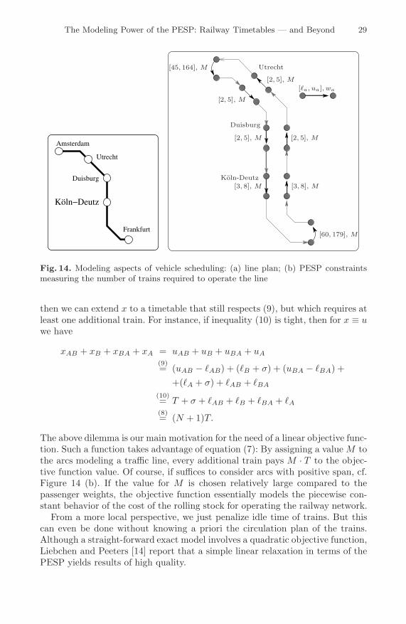
Consider for example the hourly line displayed in Figure 14 (a). Assume theminimal travel times between the two endpoints to be 235 minutes for eachdirection. Given strict minimal turnover times of 45 and 60 minutes, respectively,the minimal number of vehicles required to operate this line is precisely
N :=⌈
160
(235 + 235 + 45 + 60)⌉
= 10.
A timetable which lets the trains leave at the full hour from Frankfurt andAmsterdam can indeed be operated with only 10 trains, at least if the stoppingtimes are extended only moderately. On the contrary, a timetable in which onlythe trains starting at Frankfurt depart at minute 00, but the trains from Am-sterdam leave at minute 30 requires at least 11 vehicles. Hence, the amount ofvehicles depends on the timetable.

28 C. Liebchen and R.H. Mohring
We will analyze in which special cases pure PESP constraints are able tocontrol the number of trains required. After that, we show that a linear objectivefunction covers many more of the practical cases.
Proposition 3 (Nachtigall [20]). Consider a fixed traffic line with periodtime T . If we assume trains always to serve only this line, and if we do notallow to insert additional stopping time, then there exist upper bounds u for theturnover activities, such that the only feasible timetables are those which can beoperated with the minimal amount of trains.
Proof. We present a proof of this simple fact, both in order to provide the nota-tion used in the following paragraphs, and because it avoids modulo-notation.
Denote the endpoints of the line by A and B. Let �AB denote the minimaltravel time from A to B, i.e. the sum of the minimal stopping and running timesof the activities of this directed traffic line. Moreover, denote by �B the minimalamount of time a train has to stay in endpoint B between two consecutive trips.
The minimal number N of trains required to operate this line is precisely
N =⌈
�AB + �B + �BA + �A
T
⌉.
From the cycle periodicity property (3) we know that every feasible timetable xfulfills
xAB + xB + xBA + xA = zT, (7)
for some z ∈ Z. Hence, we must ensure z = N . To that end, consider the slack
σ := NT − (�AB + �B + �BA + �A) (8)
of this traffic line, implying (xA − �A) + (xB − �B) = σ. But since σ < T , bysetting
uA := �A + σ (9)
we even ensure xAB + xB + xBA + xA < (N + 1)T . �
Let us now analyze the case in which additional stopping times may be inserted,i.e. uAB > �AB. We will show that together with the constraints (9), sometimetables which require an additional train may become feasible.
On the one hand, consider a timetable for which we have x ≡ � for all activities,except for the turnover time in one endpoint. This timetable can still be operatedwith the minimal number of trains, showing that decreasing the value (9) for uA
would cut off timetables we seek for.On the other hand, assume xAB = uAB and xBA = uBA. If
(uAB − �AB) + (uBA − �BA) + σ ≥ T, (10)
The Modeling Power of the PESP: Railway Timetables — and Beyond 29
Amsterdam
Frankfurt
Utrecht
Duisburg
Köln−Deutz
Koln-Deutz
Duisburg
Utrecht
[�a, ua], wa
[3, 8], M
[2, 5], M
[2, 5], M
[45, 164], M
[2, 5], M
[2, 5], M
[3, 8], M
[60, 179], M
Fig. 14. Modeling aspects of vehicle scheduling: (a) line plan; (b) PESP constraintsmeasuring the number of trains required to operate the line
then we can extend x to a timetable that still respects (9), but which requires atleast one additional train. For instance, if inequality (10) is tight, then for x ≡ uwe have
xAB + xB + xBA + xA = uAB + uB + uBA + uA
(9)= (uAB − �AB) + (�B + σ) + (uBA − �BA) +
+(�A + σ) + �AB + �BA
(10)= T + σ + �AB + �B + �BA + �A
(8)= (N + 1)T.
The above dilemma is our main motivation for the need of a linear objective func-tion. Such a function takes advantage of equation (7): By assigning a value M tothe arcs modeling a traffic line, every additional train pays M · T to the objec-tive function value. Of course, if suffices to consider arcs with positive span, cf.Figure 14 (b). If the value for M is chosen relatively large compared to thepassenger weights, the objective function essentially models the piecewise con-stant behavior of the cost of the rolling stock for operating the railway network.
From a more local perspective, we just penalize idle time of trains. But thiscan even be done without knowing a priori the circulation plan of the trains.Although a straight-forward exact model involves a quadratic objective function,Liebchen and Peeters [14] report that a simple linear relaxation in terms of thePESP yields results of high quality.

30 C. Liebchen and R.H. Mohring
Very recently, Nyhave, Hove, and Clausen [22] proposed an integer linearmodel to precisely count the number of trains required to operate a timetable,even if trains are allowed to switch lines in their endpoints. This approach doesnot depend on additional assumptions as synchronization constraints or pre-defined time-windows for turnaround times, as they were used by Peeters [26]. Inthe sequel, we translate their ideas into the PESP plus some additional variablesand constraints.
Consider a station S that is a terminus for the two lines 1 and 2. Denote byai and di the arrival and departure events in station S of line i. We introducethe following arcs
a11 = (a1, d1) and a22 = (a2, d2),a12 = (a1, d2) and a21 = (a2, d1).
The effective waiting times for the trains in S are x11 + x22 if trains stay ontheir lines, or x12 + x12 if trains switch lines. Notice that (a11, a21, a22, a12) is anoriented cycle. In particular, there exists some z ∈ Z such that
x11 + x22 = x12 + x21 + zT.
In most cases, we have �a11 = �a12 and �a21 = �a22 . Then, we even know thatthere exists some r ∈ [0, T ) and b1, b2 ∈ {0, 1} such that
r = x11 + x22 − b1 · T = x12 + x21 − b2 · T.
Hence, in an optimal vehicle schedule the total effective waiting time in station Samounts to r+min{b1, b2}·T . To obtain a MIP-formulation, we introduce a new(rational) variable w and require
w ≥ b1 + b2 − 1 and w ≥ 0.
Finally, station S contributes
M · (r + w · T )
to the objective function, where M again denotes the cost factor for vehiclewaiting time.
5.2 Aspects of Line Planning
Our main idea for letting PESP solvers even take decisions of line planning isto combine — or match — pre-defined line-segments. To that end, we will makeintensive use of disjunctive constraints. Unfortunately, we will only be able toensure symmetric line plans if we require symmetry also within the stationswhere lines are matched.
We are aware of only one other approach for integrating the planning phases ofline planning, timetabling and vehicle scheduling ([32]). Whereas that approachis based on the assumption that the line plan contains no cycles, our ideas do not
The Modeling Power of the PESP: Railway Timetables — and Beyond 31
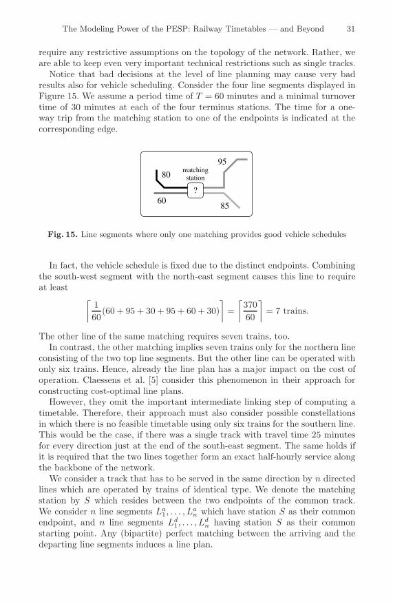
require any restrictive assumptions on the topology of the network. Rather, weare able to keep even very important technical restrictions such as single tracks.
Notice that bad decisions at the level of line planning may cause very badresults also for vehicle scheduling. Consider the four line segments displayed inFigure 15. We assume a period time of T = 60 minutes and a minimal turnovertime of 30 minutes at each of the four terminus stations. The time for a one-way trip from the matching station to one of the endpoints is indicated at thecorresponding edge.
95matching
station
8560
80
?
Fig. 15. Line segments where only one matching provides good vehicle schedules
In fact, the vehicle schedule is fixed due to the distinct endpoints. Combiningthe south-west segment with the north-east segment causes this line to requireat least
⌈160
(60 + 95 + 30 + 95 + 60 + 30)⌉
=⌈
37060
⌉= 7 trains.
The other line of the same matching requires seven trains, too.In contrast, the other matching implies seven trains only for the northern line
consisting of the two top line segments. But the other line can be operated withonly six trains. Hence, already the line plan has a major impact on the cost ofoperation. Claessens et al. [5] consider this phenomenon in their approach forconstructing cost-optimal line plans.
However, they omit the important intermediate linking step of computing atimetable. Therefore, their approach must also consider possible constellationsin which there is no feasible timetable using only six trains for the southern line.This would be the case, if there was a single track with travel time 25 minutesfor every direction just at the end of the south-east segment. The same holds ifit is required that the two lines together form an exact half-hourly service alongthe backbone of the network.
We consider a track that has to be served in the same direction by n directedlines which are operated by trains of identical type. We denote the matchingstation by S which resides between the two endpoints of the common track.We consider n line segments La
1, . . . , Lan which have station S as their common
endpoint, and n line segments Ld1, . . . , L
dn having station S as their common
starting point. Any (bipartite) perfect matching between the arriving and thedeparting line segments induces a line plan.

32 C. Liebchen and R.H. Mohring
But from the perspective of timetabling, there are only n arrival eventsa1, . . . , an as well as n departure events d1, . . . , dn visible. Hence, we must deduceonly from their arrival times πai and their departure times πdj which arrivingline segment La
i should be matched with which departing line segment Ldj .
This can be done in a canonical way, if we choose the matching station S suchthat it has only one track in the direction of the line segments we consider. Ifnecessary, we add an artificial station in the middle of some track. Then, at mostone train can be in S at the same time. Timetables respecting this constraintcan be characterized very easily as follows.
Definition 1 (Alternating timetable). For a fixed station S and a fixed di-rection, a periodic timetable π with n pairwisely different arrival times 0 ≤ πa1 <· · · < πan < T and n pairwisely different departure times 0 ≤ πd1 < · · · < πdn <T is called alternating at S, if either πai ≤ πdi < πai+1 for every i = 1, . . . , n,or πdi < πai ≤ πdi+1 for every i = 1, . . . , n, where we define π·n+1 := π·1 + T .
Lemma 6. A timetable π ensures that there is always at most one train atstation S if and only if it is alternating at S.
Hence, for an alternating periodic timetable, we combine the arriving line seg-ment La
i with the departing line segment Ldj , if and only if the latter marks
the unique first possible departure. In the sequel, we will give PESP constraintsensuring every feasible timetable to be alternating at S. Thus, every feasibletimetable will encode some unique matching and the associated line plan.
The first two sets of constraints ensure the minimal headway d in front of andbehind the matching station S:
∀ i, j ∈ {1, . . . , n} : πaj − πai ∈ [d, T − d]T , (11)∀ i, j ∈ {1, . . . , n} : πdj − πdi ∈ [d, T − d]T . (12)
Notice that (11) and (12) can only be fulfilled if 0 ≤ d ≤ Tn . Moreover, we relate
arrival events to departure events by the following disjunctive constraints
∀ i, j ∈ {1, . . . , n} : πdj − πai ∈ [0, T − d + h]T , (13)∀ i, j ∈ {1, . . . , n} : πdj − πai ∈ [d, T + h]T , (14)
where we denote by h the maximal stopping time for a train at station S. To-gether, these constraints (13) and (14) yield
(πdj − πai) mod T ∈ [0, h] ∪ [d, T − d + h]. (15)
Trivially, 0 ≤ h < d is necessary for every feasible timetable π to be alternatingat S.
Theorem 3. Let π be a timetable respecting constraints (11) to (14). Then forevery departure event dj, there exists a unique arrival event ai satisfying
πdj − πai ∈ [0, h]T , (16)
if and only if h < (n + 1)d − T .

The Modeling Power of the PESP: Railway Timetables — and Beyond 33
Since 0 ≤ h, from h < (n + 1)d − T we conclude Tn+1 < d.
Proof. “⇒”: We assume h ≥ (n + 1)d − T . Since d = Tn would imply h ≥ d, we
must only investigate the case that d < Tn . We will construct a timetable which
respects the constraints (11) to (14), but which contradicts (16).Define πai := (i−1)d, for all i = 1, . . . , n, and πdj := j ·d, for all j = 1, . . . , n.
By construction, all the constraints are satisfied. However, since πan +h < n ·d =πdn , for departure πdn none of the arrival events fulfills (16), q.e.d.
“⇐”: We assume there exists a timetable π having one departure event d0such that
∀ i = 1, . . . , n : (πd0 − πai) mod T > h,
but which respects the constraints (11) to (14). We may assume w.l.o.g. thatfor the cyclic predecessor arrival a1 of d0 we have πa1 = 0. As π is feasible, itsatisfies (15). From our assumption, we conclude d ≤ πd0 and πd0 +(d−h) ≤ πa2 ,and hence πa2 −πa1 ≥ 2d−h. Event a1 also takes place at time T . For notationalconvenience, we define πan+1 := T . With this notation, we have πai+1 − πai ≥ d,for all i = 2, . . . , n. By the definition of πan+1 , we know that
n∑
i=1
(πai+1 − πai) = πan+1 − πa1 = T.
Summing up the lower bounds yields T ≥ (n + 1)d − h, which contradicts thehypothesis of Theorem 3. �
Corollary 1. If h < (n+1)d−T , then every timetable which respects constraints(11) to (14) is an alternating timetable.
In Figure 16, we provide an example for the easiest case, namely matching twolines. As usual, we assume the period time to be 60 minutes.
Remark 2. There are of course alternating periodic timetables in the case d ≤T
n+1 . PESP solvers are able to detect even those, if we were able to pre-definesufficiently many empty slots. By an “empty slot” we understand an artificialline which we have to schedule in the same way as the original lines, herebyseparating the lines before and after the empty slot.
In more detail, let us assume that Tn∗+1 < d ≤ T
n∗ for some n∗ > n, andthat h satisfies the assumptions of Theorem 3 for n∗. We then introduce n∗ − nartificial dummy arrival and departure events ai and di, i = n + 1, . . . , n∗. Toprevent the original line segments from being matched with an artificial event,we require πdi − πai ∈ [0, h] for all i = n + 1, . . . , n∗.
By construction, the only feasible timetables let the original arrivals and de-partures alternate. However, perfectly balanced timetables, i.e. πai := (i − 1)T
n ,are infeasible under these settings if n∗ < 2n, since they do not provide n∗ − nempty slots.
Recall that so far we have considered only one direction. Hence, there is nomechanism yet to bind the matching of one direction to that of the opposite
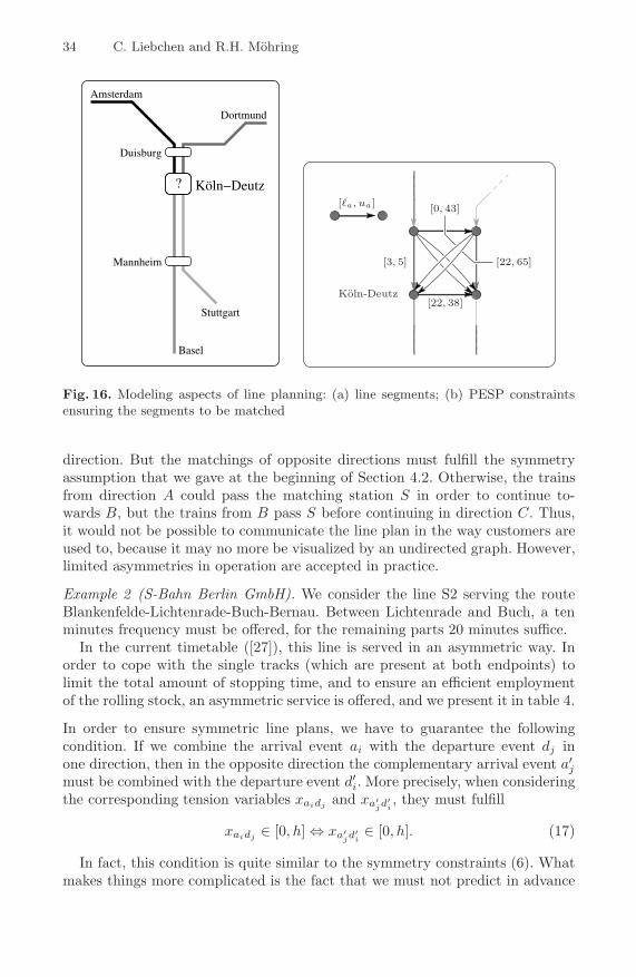
34 C. Liebchen and R.H. Mohring
Amsterdam
Dortmund
Basel
Stuttgart
Duisburg
Mannheim
Köln−Deutz?
Koln-Deutz[22, 38]
[3, 5]
[0, 43]
[22, 65]
[�a, ua]
Fig. 16. Modeling aspects of line planning: (a) line segments; (b) PESP constraintsensuring the segments to be matched
direction. But the matchings of opposite directions must fulfill the symmetryassumption that we gave at the beginning of Section 4.2. Otherwise, the trainsfrom direction A could pass the matching station S in order to continue to-wards B, but the trains from B pass S before continuing in direction C. Thus,it would not be possible to communicate the line plan in the way customers areused to, because it may no more be visualized by an undirected graph. However,limited asymmetries in operation are accepted in practice.
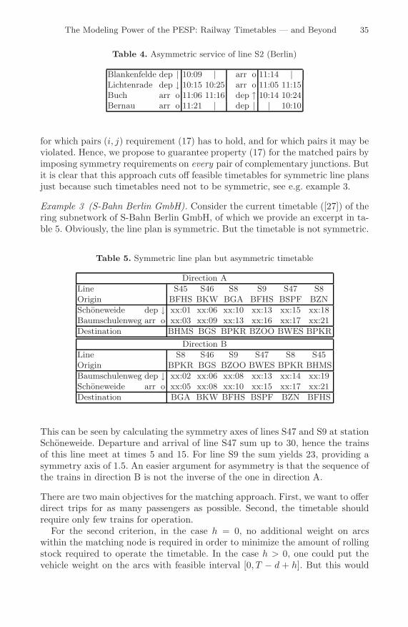
Example 2 (S-Bahn Berlin GmbH). We consider the line S2 serving the routeBlankenfelde-Lichtenrade-Buch-Bernau. Between Lichtenrade and Buch, a tenminutes frequency must be offered, for the remaining parts 20 minutes suffice.
In the current timetable ([27]), this line is served in an asymmetric way. Inorder to cope with the single tracks (which are present at both endpoints) tolimit the total amount of stopping time, and to ensure an efficient employmentof the rolling stock, an asymmetric service is offered, and we present it in table 4.
In order to ensure symmetric line plans, we have to guarantee the followingcondition. If we combine the arrival event ai with the departure event dj inone direction, then in the opposite direction the complementary arrival event a′
j
must be combined with the departure event d′i. More precisely, when consideringthe corresponding tension variables xaidj and xa′
jd′i, they must fulfill
xaidj ∈ [0, h] ⇔ xa′jd′
i∈ [0, h]. (17)
In fact, this condition is quite similar to the symmetry constraints (6). Whatmakes things more complicated is the fact that we must not predict in advance
The Modeling Power of the PESP: Railway Timetables — and Beyond 35
Table 4. Asymmetric service of line S2 (Berlin)
Blankenfelde dep | 10:09 | arr o 11:14 |Lichtenrade dep ↓ 10:15 10:25 arr o 11:05 11:15Buch arr o 11:06 11:16 dep ↑ 10:14 10:24Bernau arr o 11:21 | dep | | 10:10
for which pairs (i, j) requirement (17) has to hold, and for which pairs it may beviolated. Hence, we propose to guarantee property (17) for the matched pairs byimposing symmetry requirements on every pair of complementary junctions. Butit is clear that this approach cuts off feasible timetables for symmetric line plansjust because such timetables need not to be symmetric, see e.g. example 3.
Example 3 (S-Bahn Berlin GmbH). Consider the current timetable ([27]) of thering subnetwork of S-Bahn Berlin GmbH, of which we provide an excerpt in ta-ble 5. Obviously, the line plan is symmetric. But the timetable is not symmetric.
Table 5. Symmetric line plan but asymmetric timetable
Direction ALine S45 S46 S8 S9 S47 S8Origin BFHS BKW BGA BFHS BSPF BZNSchoneweide dep ↓ xx:01 xx:06 xx:10 xx:13 xx:15 xx:18Baumschulenweg arr o xx:03 xx:09 xx:13 xx:16 xx:17 xx:21Destination BHMS BGS BPKR BZOO BWES BPKR
Direction BLine S8 S46 S9 S47 S8 S45Origin BPKR BGS BZOO BWES BPKR BHMSBaumschulenweg dep ↓ xx:02 xx:06 xx:08 xx:13 xx:14 xx:19Schoneweide arr o xx:05 xx:08 xx:10 xx:15 xx:17 xx:21Destination BGA BKW BFHS BSPF BZN BFHS
This can be seen by calculating the symmetry axes of lines S47 and S9 at stationSchoneweide. Departure and arrival of line S47 sum up to 30, hence the trainsof this line meet at times 5 and 15. For line S9 the sum yields 23, providing asymmetry axis of 1.5. An easier argument for asymmetry is that the sequence ofthe trains in direction B is not the inverse of the one in direction A.
There are two main objectives for the matching approach. First, we want to offerdirect trips for as many passengers as possible. Second, the timetable shouldrequire only few trains for operation.
For the second criterion, in the case h = 0, no additional weight on arcswithin the matching node is required in order to minimize the amount of rollingstock required to operate the timetable. In the case h > 0, one could put thevehicle weight on the arcs with feasible interval [0, T − d + h]. But this would
36 C. Liebchen and R.H. Mohring
no longer yield the desired exact piecewise-constant behavior of the objective,because some double counting can appear.
For maximizing the number of direct travelers, we consider the number ofpassengers wij starting their trip before the common track on a train coveringline segment La
i , and finishing their trip after the common endpoint on a traincovering line segment Ld
j . The value wij is added to the weight of the arc a =(ai, dj) with �a = 0 and ua = [0, T − d + h]. The resulting cost coefficients inthe objective function make even sense for pairs of line segments which are notmatched, because long changeover times of many passengers are penalized.
Notice that the values wij are only well-defined if the two line segments donot serve a second matching station. This shows that the decisions to be takenwithin a matching station are of a rather local nature.
Summarizing, there are important scenarios in which the PESP can integraterelevant aspects of line planning into a model suited for timetabling and keyissues of vehicle scheduling. This is in particular the case if symmetric timetablesand balanced sequences along the common tracks, i.e. d > T
n+1 , are requestedfor their own sake. Moreover, we observed that the larger the distance betweentwo matching stations, the more reliable the passenger weight that we propose.
We think that fast train networks of European agglomerations, such as Frank-furt, Munich, or Paris (RER), are well-suited candidates for this approach.There, many passengers might have their origin or destination somewhere onthe backbone route, and balanced sequences must be ensured due to the largenumber of lines per period.
5.3 Aspects of Network Planning
We propose to also model two questions which arise in network planning withinthe PESP: the extension of existing tracks, and thus lines, beyond their currentendpoints, and the construction of faster tracks as substitution for existing ones.Taking into account that, in these questions, we have to select one option out ofa small number of disjoint options, it is evident that we will make intensive use ofdisjunctive constraints, cf. Section 3.3. Recall that there, we already discussed theintroduction of optinal additional stops. With appropriate weights that reflectamortisation—see below—these may also cover the construction of new stationsalong an existing track.
We only discuss the construction of faster tracks in detail. But the readerwill have no difficulty to adapt our suggestions to the very similar task of theextension of tracks.
In Figure 17, we provide a constraint graph which offers the option of a newtrack between Aachen and Koln, being then part of the European high-speed linePBK (Paris-Brussels-Koln). We provide the status quo, with one intermediatestop, only for illustration purposes. In the future, we have the option to eitheruse the current tracks, thus keeping a trip time of 38 minutes, or to establishthe new high-speed track, hereby reducing the trip time down to 26 minutes.
To define appropriate weights for the arcs, we have to take into account threedifferent types of objectives: The number of customers c who profit from a new
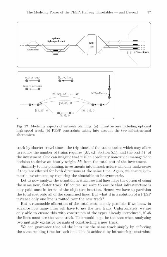
The Modeling Power of the PESP: Railway Timetables — and Beyond 37
Köln−Deutz
Köln
HbfAachen Hbf
high−speed trackoptional
Koln-Deutz
status quo
future options
[21, 21], 0
[2, 2], 0
[15, 15], 0
[26, 38], M + c − M ′
[38, 86], 0
[�a, ua], wa
Fig. 17. Modeling aspects of network planning: (a) infrastructure including optionalhigh-speed track; (b) PESP constraints taking into account the two infrastructuralalternatives
track by shorter travel times, the trip times of the trains trains which may allowto reduce the number of trains requires (M , c.f. Section 5.1), and the cost M ′ ofthe investment. One can imagine that it is an absolutely non-trivial managementdecision to derive an hourly weight M ′ from the total cost of the investment.
Similarly to line planning, investments into infrastructure will only make senseif they are effected for both directions at the same time. Again, we ensure sym-metric investments by requiring the timetable to be symmetric.
Let us now analyze the situation in which several lines have the option of usingthe same new, faster track. Of course, we want to ensure that infrastructure isonly paid once in terms of the objective function. Hence, we have to partitionthe total cost onto all of the concerned lines. But what if in a solution of a PESPinstance only one line is routed over the new track?
But a reasonable allocation of the total costs is only possible, if we know inadvance how many lines will have to use the new track. Unfortunately, we areonly able to ensure this with constraints of the types already introduced, if allthe lines must use the same track. This would, e.g., be the case when analyzingtwo mutually exclusive variants of constructing a new track.
We can guarantee that all the lines use the same track simply by enforcingthe same running time for each line. This is achieved by introducing constraints

38 C. Liebchen and R.H. Mohring
of type (6). But notice that in this case we cheat a bit, because those constraintsno longer relate only pairs of complementary arcs to each other. . . Anyway, theMIP formulation of this even slightly more extended model incorporates manyof the computational aspects of the pure PESP model.
6 Conclusion
Our discussion of the PESP model shows that it has a great modeling power andextendability. We have demonstrated that many non-standard requirements forperiodic timetables and also important aspects of other – traditionally separate –planning phases can be integrated into the PESP. Figure 18 displays the gain bythis modeling power over the traditional use of the PESP displayed in Figure 1.
Network Planning
Line Planning
Timetabling
Vehicle Scheduling
Crew Scheduling
PESP model
Fig. 18. Planning phases covered by the PESP with our contribution
Interestingly, this integration into the PESP has been possible without seem-ingly complicating it too much. In all cases, we obtained mixed integer programsthat still have the characteristics of a PESP. Hence we believe that these ex-tended models stay computationally tractable also for networks of relevant sizes.So far, our belief is confirmed by a confidential study for S-Bahn Berlin GmbHfor two of its three major subnetworks.
We therefore hope that these models, through their integrative approach tovehicle scheduling, timetabling, line planning, and infrastructure planning, willeventually lead to better decision making in practice.
Acknowledgments
We want to thank the staff of Deutsche Bahn AG, S-Bahn Berlin GmbH, andBerliner Verkehrsbetriebe (BVG) for providing us with both real-world dataand very detailed requirements of their specific periodic timetabling problems.Moreover, we thank the referees for their very detailed suggestions.
The Modeling Power of the PESP: Railway Timetables — and Beyond 39
References
1. Bollobas, B.: Modern Graph Theory. Graduate Texts in Mathematics, vol. 184(2nd printing) Springer, Heidelberg (2002)
2. Borndorfer, R., Grotschel, M., Pfetsch, M.E.: A path-based model for line planningin public transport. Technical Report 05-18, Zuse Institute, Berlin (2005)
3. Borndorfer, R., Lobel, A., Weider, S.: Integrierte Umlauf- und Dienstplanungim offentlichen Nahverkehr. In: HEUREKA ’02: Optimierung in Transport undVerkehr, Tagungsbericht, number 002/72. FGSV Verlag (in German) (2002)
4. Bussieck, M.R., Winter, T., Zimmermann, U.: Discrete optimization in public railtransport. Mathematical Programming B 79, 415–444 (1997)
5. Claessens, M.T., van Dijk, N.M., Zwanefeld, P.J.: Cost optimal allocation of railpassenger lines. European Journal of Operational Research 110(3), 474–489 (1998)
6. Engelhardt-Funke, O., Kolonko, M.: Analysing stability and investments in railwaynetworks using advanced evolutionary algorithms. International Transactions inOperational Research 11, 381–394 (2004)
7. Grotschel, M., Lobel, A., Volker, M.: Optimierung des Fahrzeugumlaufs imoffentlichen Nahverkehr. In: Hoffmann, K.H., Jager, W., Lohmann, T., Schunck,H. (eds.) Mathematik - Schlusseltechnologie fur die Zukunft, Springer, Heidelberg(in German) (1997)
8. Haase, K., Desaulniers, G., Desrosiers, J.: Simultaneous vehicle and crew schedulingin urban mass transit systems. Transportation Science 35(3), 286–303 (2001)
9. Krista, M.: Verfahren zur Fahrplanoptimierung am Beispiel der Synchronzeiten.Ph.D. thesis, Technische Universitat Braunschweig (in German) (1997)
10. Kroon, L.G., Peeters, L.W.P.: A variable trip time model for cyclic railwaytimetabling. Transportation Science 37, 198–212 (2003)
11. Leuschel, I.: Der Fernverkehrsfahrplan 2003 der Deutschen Bahn AG. Eisenbahn-technische Rundschau (In German) 51(7–8), 452–464 (2002)
12. Liebchen, C.: Finding short integral cycle bases for cyclic timetabling. In: Di Bat-tista, G., Zwick, U. (eds.) ESA 2003. LNCS, vol. 2832, pp. 715–726. Springer,Heidelberg (2003)
13. Liebchen, C.: Symmetry for periodic railway timetables. Electronic Notes in The-oretical Computer Science 92, 34–51 (2004)
14. Liebchen, C., Peeters, L.: Some practical aspects of periodic timetabling. In: Cha-moni, P., Leisten, R., Martin, A., Minnemann, J., Stadtler, H. (eds.) OperationsResearch 2001, Springer, Heidelberg (2002)
15. Liebchen, C., Proksch, M., Wagner, F.H.: Performance of algorithms for pe-riodic timetable optimization. In: Hickman, M. (ed.) Computer-Aided TransitScheduling— Proceedings of the Ninth International Workshop on Computer-Aided Scheduling of Public Transport. Lecture Notes in Economics and Mathe-matical Systems, Springer, Heidelberg (to appear, 2005)
16. Lindner, T.: Train Schedule Optimization in Public Rail Transport. Ph.D. thesis,Technische Universitat Braunschweig (2000)
17. Rhein-Main Verkehrsverbund: Fahrplanbuch Gesamtausgabe (gultig ab 14. Dezem-ber 2003) (2003)
18. Nachtigall, K.: A branch and cut approach for periodic network programming.Hildesheimer Informatik-Berichte 29, Universitat Hildesheim (1994)
19. Nachtigall, K.: Cutting planes for a polyhedron associated with a periodic network.Institutsbericht IB 112-96/17, Deutsche Forschungsanstalt fur Luft- und Raum-fahrt e.V (July 1996)
40 C. Liebchen and R.H. Mohring
20. Nachtigall, K.: Periodic Network Optimization and Fixed Interval Timetables. Ha-bilitation thesis, Universitat Hildesheim (1998)
21. Nachtigall, K., Voget, S.: A genetic algorithm approach to periodic railway syn-chronization. Computers and Operations Research 23(5), 453–463 (1996)
22. Nielsen, M.N., Hove, B., Clausen, J.: Constructing periodic timetables using MIP—a case study from DSB S-train. International Journal of Operations Research, 1(2005)
23. Odijk, M.A.: Construction of periodic timetables, Part 1: A cutting plane algo-rithm. Technical Report 94-61, TU Delft (1994)
24. Odijk, M.A.: A constraint generation algorithm for the construction of periodicrailway timetables. Transportation Research B 30(6), 455–464 (1996)
25. Peeters, L.W.P.: Personal Communication (2000)26. Peeters, L.W.P.: Cyclic Railway Timetable Optimization. Ph.D. thesis, Erasmus
Universiteit Rotterdam (2003)27. S-Bahn Berlin GmbH: S-Bahn-Fahrplan (gultig ab 16. Juni 2003) (2003)28. Schrijver, A.: Theory of Linear and Integer Programming, 2nd edn. Wiley, Chich-
ester (1998)29. Schrijver, A., Steenbeek, A.G.: Dienstregelingontwikkeling voor Nederlandse
Spoorwegen N.S. Rapport Fase 1, Centrum voor Wiskunde en Informatica (Okto-ber 1993)
30. Serafini, P., Ukovich, W.: A mathematical model for periodic scheduling problems.SIAM Journal on Discrete Mathematics 2(4), 550–581 (1989)
31. van den Berg, J.H.A., Odijk, M.A.: DONS: Computer aided design of regular ser-vice timetables. In: Murthy, T.K.S., Mellitt, B., Brebbia, C.A., Sciutto, G., Sone,S. (eds.) Computers in Railways IV (COMPRAIL)—vol. 2: Railway Operations.WIT Press (1994)
32. Volker, M.: Ein multikriterieller Algorithmus zur automatisierten Bus-liniennetzplanung. Lecture on the OR Workshop Optimierung im offentlichenNahverkehr (2003)