The Model Object in EViews - World Banksiteresources.worldbank.org/INTPSIA/Resources/... · In...
60
The Model Object in EViews B. Essama-Nssah Poverty Reduction Group (PRMPR) The World Bank Washington, DC October 12, 2005
-
Upload
duongduong -
Category
Documents
-
view
220 -
download
0
Transcript of The Model Object in EViews - World Banksiteresources.worldbank.org/INTPSIA/Resources/... · In...

The Model Object in EViews
B. Essama-NssahPoverty Reduction Group (PRMPR)
The World BankWashington, DC
October 12, 2005

2
ForewordA “logical picture” differs from an ordinary picture in that it need not look the least bit like its object. Its relation to the object is not that of a copy, but of analogy. …The great value of analogy is that by it, and it alone, we are led to seeing a single “logical form” in things which may be entirely discrepant as to content.
Langer (1967)

3
Topics
1. What is a Model?DefinitionExample
2. Specification3. Parameter Estimation4. Model Set-Up and Solution5. Types of Simulations6. Scenario Implementation7. Hands-On Exercise

4
What is a Model?Definition of Model
A model is a logical picture (structural expression) of a phenomenon. A quantitative model is usually represented by a set of equations that jointly describe relationships among a group of variables.In EViews, the model object combines such equations into a single entity that may be used to create a joint forecast or a simulation of all endogenous variables of the model.

5
What is a Model?Example: Keynesian Model of Income Determination (A framework for analyzing the interaction between the financial and the real sides of the economy).
Aggregate demand determines the equilibrium level of output.Real economy determines level of income which affects the demand for money, a financial variable.The financial sector determines the interest rates which affect investment in the real economy.A static IS-LM model is a reduced-form representation of macroeconomic balance through a simultaneous equilibrium of the goods and the money markets.
6
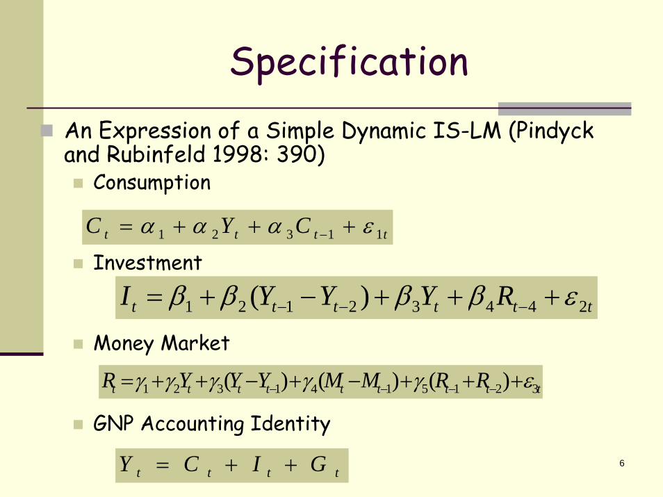
SpecificationAn Expression of a Simple Dynamic IS-LM (Pindyck and Rubinfeld 1998: 390)
Consumption
Investment
Money Market
GNP Accounting Identity
tttt CYC 11321 εααα +++= −
tttttt RYYYI 24432121 )( εββββ +++−+= −−−
ttttttttt RRMMYYYR 3215141321 )()()( εγγγγγ +++−+−++= −−−−
tttt GICY ++=
7
SpecificationEquation list and key variables
First equation describes an autoregressive consumption function.Investment is related to GNP and interest rate in the second equation.The third equation represents the money market. It relates interest rate to GNP and the money supply.Last equation may be interpreted as equilibrium condition for the goods market.
Typical economic models include two categories of equations: (1) behavioral; (2) equilibrium conditions
8
Parameter EstimationNumerical implementation requires that we assign numerical values to structural parameters of the model.For econometric models we resort to estimation.Appropriate method of estimation depends on underlying stochastic structure of the model and the desirable properties we would like the estimator to have.Recall the benchmark case of the classical linear model:
Identification condition (Greene 2000): lack of multicollinearity, and there are at least as many observations as parameters to be estimated.

9
Parameter EstimationClassical case
Strict exogeneity (Hayashi 2000) holds (i.e. no observations on any explanatory variable convey information of the expected value of the random disturbance). Hence the expectation of the disturbance conditional on observables is zero. So, strict exogeneity implies that, for all observations, the explanatory variables are orthogonal to the random disturbances.Spherical error variance (Greene 2000): Homoskedasticity (constant variance) and no correlation between observations.Under these circumstances, OLSE is a feasible and optimal method of estimation among all linear estimators. Identification ensures feasibility, while the rest of the assumptions brings optimality in terms of unbiasedness (hitting the target on average) and efficiency (minimum variance).

10
Parameter EstimationAlso, in large samples, OLSE is consistent in the sense that it converges, in probability to the true value of the parameter. (Both unbiasedness and consistency hinge on the assumption of strict exogeneity).
Implications of SimultaneityConsider a very simple model of national income determination where variables are measured in deviations from sample means (Pindyck and Rubinfeld 1998:341)
The OLSE for the marginal propensity to consume is:
ttttttt gicyyc ++=+= ;εβ
∑∑
∑∑
+==
tt
ttt
tt
ttt
y
y
y
ycb 22
εβ
11
Parameter EstimationImplications of Simultaneity
Above reveals that explanatory variable yt is related to the disturbance εt via ct. Hence strict exogeneity is lost and we can no longer claim that the OLSE is unbiased and consistent. Any remedy?
IdentificationIdentification is a prerequisite for estimationPosed in terms of the relationship between structural and reduced-form parameters, the issue is whether we can obtain values of the structural parameters from reduced-form estimates.An equation is unidentified if there is no way of
estimating all the structural parameters from reduced-form estimates, otherwise the equation is identified.

12
Parameter EstimationIdentification
It is exactly identified if there is a unique set of values for structural parameters in terms of the reduced-form ones. If more than one value is obtainable for some parameters, then the equation is overidentified. Order condition for identification (necessary, but not sufficient): The number of predetermined variables (exogenous and lagged endogenous variables) excluded from the equation must be at least equal to the number of included endogenous variables minus one (Pindyck and Rubinfeld 1998:245).
13
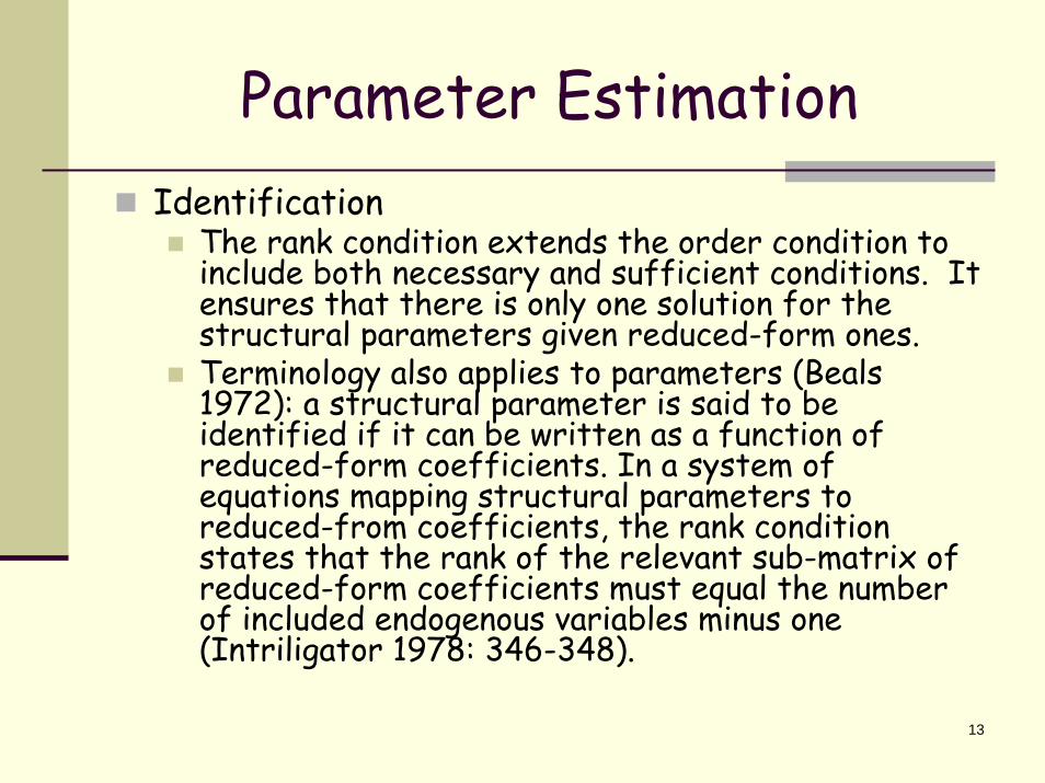
Parameter EstimationIdentification
The rank condition extends the order condition to include both necessary and sufficient conditions. It ensures that there is only one solution for the structural parameters given reduced-form ones.Terminology also applies to parameters (Beals 1972): a structural parameter is said to be identified if it can be written as a function of reduced-form coefficients. In a system of equations mapping structural parameters to reduced-from coefficients, the rank condition states that the rank of the relevant sub-matrix of reduced-form coefficients must equal the number of included endogenous variables minus one (Intriligator 1978: 346-348).
14
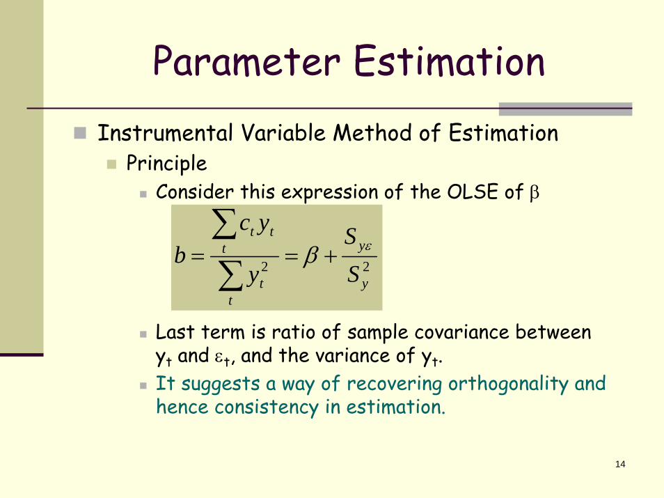
Parameter EstimationInstrumental Variable Method of Estimation
PrincipleConsider this expression of the OLSE of β
Last term is ratio of sample covariance between yt and εt, and the variance of yt.It suggests a way of recovering orthogonality and hence consistency in estimation.
22y
y
tt
ttt
SS
y
ycb εβ +==
∑∑

15
Parameter EstimationInstrumental Variable Method of Estimation
If there is a variable xt highly correlated with yt but uncorrelated with εt, then use it as instrument to get:
Choice of InstrumentsMost common practice: use 2SLS with predetermined variables as instruments.Predetermined variables are assumed uncorrelated with error terms. Their inclusion in model means they are correlated with endogenous variables.
yx
x
ttt
ttt
IV SS
xy
xcb εβ +==
∑∑

16
Parameter EstimationInstrumental Variable Method of Estimation
2SLSRegress included endogenous variable on predetermined variables.Use fitted value of endogenous as instrument in IV expression or regress the dependent variable on fitted value of included endogenous and the relevant predetermined variables.
∑
∑
∑
∑==
tt
ttt
ttt
ttt
sls
y
yc
yy
ycb ^
2
^
^
^
2

17
Parameter EstimationInstrumental Variable Method of Estimation
Generalized Method of Moments (GMM)Member of the IV family of estimators that relies on a set of orthogonality conditions and does not require specification of the distribution of error terms.For a valid instrument xt, the orthogonality condition is:
0)]([ =− ttt ycxE β

18
Parameter EstimationInstrumental Variable Method of Estimation
Generalized Method of Moments (GMM)Sample analogue:
Hence
When
We get 2SLS
∑ =−
ttGMMtt ybcx
n0)]([1
IV
ttt
ttt
GMM bxy
xcb ==
∑∑
^
tt yx =
19
Parameter EstimationInstrumental Variable Method of Estimation
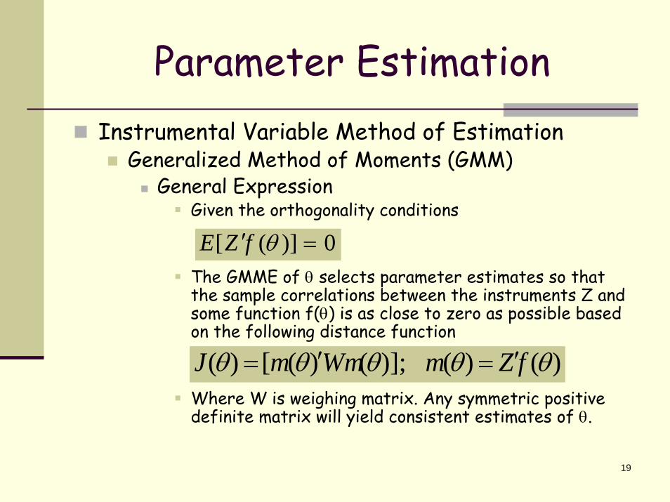
Generalized Method of Moments (GMM)General Expression
Given the orthogonality conditions
The GMME of θ selects parameter estimates so that the sample correlations between the instruments Z and some function f(θ) is as close to zero as possible based on the following distance function
Where W is weighing matrix. Any symmetric positive definite matrix will yield consistent estimates of θ.
0)]([ =′ θfZE
)()()];()([)( θθθθθ fZmWmmJ ′=′=
20
Parameter EstimationFull Information Estimation
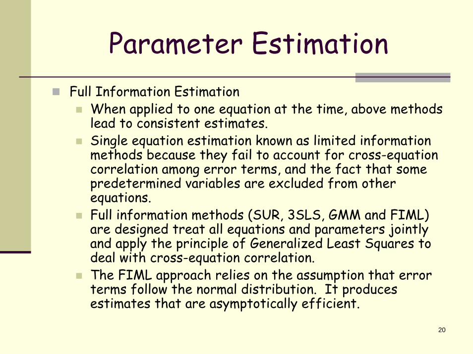
When applied to one equation at the time, above methods lead to consistent estimates.Single equation estimation known as limited information methods because they fail to account for cross-equation correlation among error terms, and the fact that some predetermined variables are excluded from other equations. Full information methods (SUR, 3SLS, GMM and FIML) are designed treat all equations and parameters jointly and apply the principle of Generalized Least Squares to deal with cross-equation correlation.The FIML approach relies on the assumption that error terms follow the normal distribution. It produces estimates that are asymptotically efficient.
21
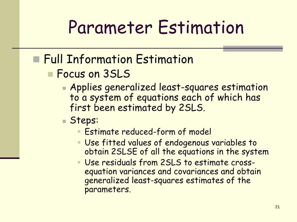
Parameter EstimationFull Information Estimation
Focus on 3SLSApplies generalized least-squares estimation to a system of equations each of which has first been estimated by 2SLS.Steps:
Estimate reduced-form of modelUse fitted values of endogenous variables to obtain 2SLSE of all the equations in the systemUse residuals from 2SLS to estimate cross-equation variances and covariances and obtain generalized least-squares estimates of the parameters.

22
Parameter Estimation
Full Information EstimationFocus on 3SLS
Link to GMM (Hayashi 2000)Under heteroskedasticity, GMM is equivalent to Full Information Instrumental Variable Estimator (FIVE).Which in turn is the 3SLSE if the set of instruments is common to all equations.If all regressors are predetermined, then 3SLSE=SURE.Which reduces to the multivariate regression when all equations have the same regressors.
23
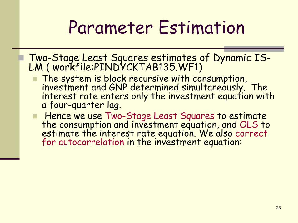
Parameter EstimationTwo-Stage Least Squares estimates of Dynamic IS-LM ( workfile:PINDYCKTAB135.WF1)
The system is block recursive with consumption, investment and GNP determined simultaneously. The interest rate enters only the investment equation with a four-quarter lag.Hence we use Two-Stage Least Squares to estimate
the consumption and investment equation, and OLS to estimate the interest rate equation. We also correctfor autocorrelation in the investment equation:
24
Parameter Estimation
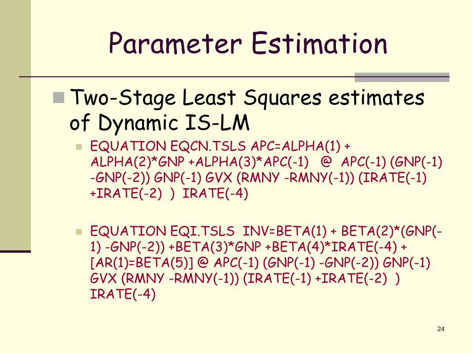
Two-Stage Least Squares estimates of Dynamic IS-LM
EQUATION EQCN.TSLS APC=ALPHA(1) + ALPHA(2)*GNP +ALPHA(3)*APC(-1) @ APC(-1) (GNP(-1) -GNP(-2)) GNP(-1) GVX (RMNY -RMNY(-1)) (IRATE(-1) +IRATE(-2) ) IRATE(-4)
EQUATION EQI.TSLS INV=BETA(1) + BETA(2)*(GNP(-1) -GNP(-2)) +BETA(3)*GNP +BETA(4)*IRATE(-4) + [AR(1)=BETA(5)] @ APC(-1) (GNP(-1) -GNP(-2)) GNP(-1) GVX (RMNY -RMNY(-1)) (IRATE(-1) +IRATE(-2) ) IRATE(-4)

25
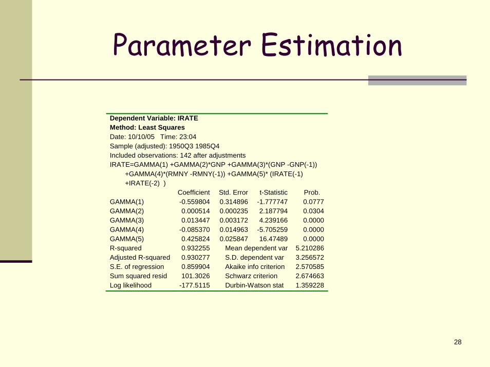
Parameter EstimationEQUATION EQR.LS IRATE=GAMMA(1) +GAMMA(2)*GNP +GAMMA(3)*(GNP -GNP(-1)) +GAMMA(4)*(RMNY -RMNY(-1)) +GAMMA(5)* (IRATE(-1) +IRATE(-2) )
26
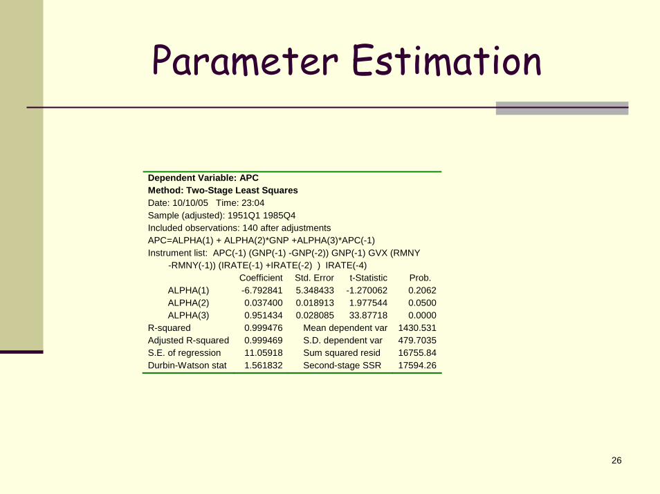
Parameter Estimation
Dependent Variable: APC Method: Two-Stage Least Squares Date: 10/10/05 Time: 23:04 Sample (adjusted): 1951Q1 1985Q4 Included observations: 140 after adjustments APC=ALPHA(1) + ALPHA(2)*GNP +ALPHA(3)*APC(-1) Instrument list: APC(-1) (GNP(-1) -GNP(-2)) GNP(-1) GVX (RMNY -RMNY(-1)) (IRATE(-1) +IRATE(-2) ) IRATE(-4)
Coefficient Std. Error t-Statistic Prob. ALPHA(1) -6.792841 5.348433 -1.270062 0.2062 ALPHA(2) 0.037400 0.018913 1.977544 0.0500 ALPHA(3) 0.951434 0.028085 33.87718 0.0000
R-squared 0.999476 Mean dependent var 1430.531 Adjusted R-squared 0.999469 S.D. dependent var 479.7035 S.E. of regression 11.05918 Sum squared resid 16755.84 Durbin-Watson stat 1.561832 Second-stage SSR 17594.26

27
Parameter EstimationDependent Variable: INV Method: Two-Stage Least Squares Date: 10/10/05 Time: 23:04 Sample (adjusted): 1951Q2 1985Q4 Included observations: 139 after adjustments Convergence achieved after 15 iterations INV=BETA(1) + BETA(2)*(GNP(-1) -GNP(-2)) +BETA(3)*GNP +BETA(4)*IRATE(-4) + [AR(1)=BETA(5)] Instrument list: APC(-1) (GNP(-1) -GNP(-2)) GNP(-1) GVX (RMNY -RMNY(-1)) (IRATE(-1) +IRATE(-2) ) IRATE(-4)
Lagged dependent variable & regressors added to instrument list
Coefficient Std. Error t-Statistic Prob. BETA(1) -62.75639 20.68087 -3.034514 0.0029 BETA(2) 0.086076 0.048132 1.788322 0.0760 BETA(3) 0.205110 0.009691 21.16394 0.0000 BETA(4) -6.284993 1.523252 -4.126036 0.0001 BETA(5) 0.765456 0.054908 13.94070 0.0000 R-squared 0.985826 Mean dependent
var 389.1424
Adjusted R-squared 0.985403 S.D. dependent var 130.2811 S.E. of regression 15.74032 Sum squared resid 33199.53 Durbin-Watson stat 1.811167 Inverted AR Roots .77
28
Parameter Estimation
Dependent Variable: IRATE Method: Least Squares Date: 10/10/05 Time: 23:04 Sample (adjusted): 1950Q3 1985Q4 Included observations: 142 after adjustments IRATE=GAMMA(1) +GAMMA(2)*GNP +GAMMA(3)*(GNP -GNP(-1)) +GAMMA(4)*(RMNY -RMNY(-1)) +GAMMA(5)* (IRATE(-1) +IRATE(-2) )
Coefficient Std. Error t-Statistic Prob. GAMMA(1) -0.559804 0.314896 -1.777747 0.0777 GAMMA(2) 0.000514 0.000235 2.187794 0.0304 GAMMA(3) 0.013447 0.003172 4.239166 0.0000 GAMMA(4) -0.085370 0.014963 -5.705259 0.0000 GAMMA(5) 0.425824 0.025847 16.47489 0.0000 R-squared 0.932255 Mean dependent var 5.210286 Adjusted R-squared 0.930277 S.D. dependent var 3.256572 S.E. of regression 0.859904 Akaike info criterion 2.570585 Sum squared resid 101.3026 Schwarz criterion 2.674663 Log likelihood -177.5115 Durbin-Watson stat 1.359228

29
Model Set-Up and Solution Declaration StatementMODEL ISLMD 'A Dynamic IS-LM ModelBring in linked equationsFOR %EQ EQCN EQI EQR
ISLMD.MERGE {%EQ}NEXT
Add inline identityISLMD.APPEND GNP=APC + INV +GVX
Note: must assign a unique endogenous variable to each equation; any non-assigned variable is considered exogenous to the model.A linked equation gets its specification from an external object e.g. estimation object (equation or system). Inline equation is specified as text in the model.

30
Model Set-Up and SolutionSolution Sample (Tracking History)SMPL 1951Q2 1985Q4
Chosen in a way that accommodates the lags involved in instruments.
Baseline solutionISLMD.SCENARIO BASELINEISLMD.SOLVE(s=d,d=s)
s=d: solution type=deterministic (not stochastic).d=s: solution dynamics=static i.e. model prediction based on actual values of exogenous and lagged endogenous variables.Default Solver: Gauss-Seidel ; Alternative: Newton
Create a Graph called HISTORYISLMD.MAKEGRAPH(a) HISTORY @ENDOG
Option a means include actuals in the graph.Could use MAKEGROUP to create a table

31
Tracking History
500
1000
1500
2000
2500
1955 1960 1965 1970 1975 1980 1985
Real Aggregate Personal ConsumptionReal Aggregate Personal Consumption (Baseline)
Real Aggregate Personal Consumption
1000
1500
2000
2500
3000
3500
4000
1955 1960 1965 1970 1975 1980 1985
Real GNP net of Exports and ImportsReal GNP net of Exports and Imports (Baseline)
Real GNP net of Exports and Imports
100
200
300
400
500
600
700
1955 1960 1965 1970 1975 1980 1985
Real Gross Domestic InvestmentReal Gross Domestic Investment (Baseline)
Real Gross Domestic Investment
0
4
8
12
16
1955 1960 1965 1970 1975 1980 1985
Interest Rate on Three-Month Treasury BillsInterest Rate on Three-Month Treasury Bills (Baseline)
Interest Rate on Three-Month Treasury Bills

32
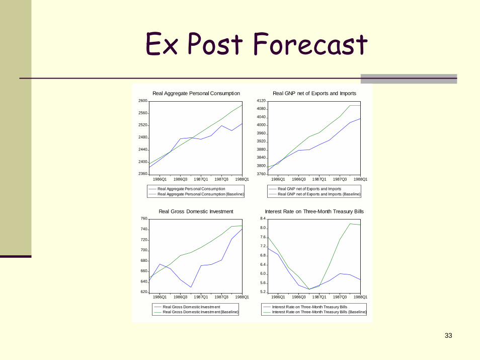
Types of SimulationsHistorical or ex post simulation: static solution based on estimation sample (see case above).Ex post forecast: dynamic based on observations outside estimation sample:SMPL 1985Q4 1988Q1ISLMD.SOLVE(s=d,d=d)
d=d invokes a dynamic simulation: values for lagged endogenous variables are obtained from previous period forecasts and not from actual historical data.
Both types of simulations (historical and ex post forecast) help evaluate ability of model to replicate actual data.
33
Ex Post Forecast
2360
2400
2440
2480
2520
2560
2600
1986Q1 1986Q3 1987Q1 1987Q3 1988Q1
Real Aggregate Personal ConsumptionReal Aggregate Personal Consumption (Baseline)
Real Aggregate Personal Consumption
3760
3800
3840
3880
3920
3960
4000
4040
4080
4120
1986Q1 1986Q3 1987Q1 1987Q3 1988Q1
Real GNP net of Exports and ImportsReal GNP net of Exports and Imports (Baseline)
Real GNP net of Exports and Imports
620
640
660
680
700
720
740
760
1986Q1 1986Q3 1987Q1 1987Q3 1988Q1
Real Gross Domestic InvestmentReal Gross Domestic Investment (Baseline)
Real Gross Domestic Investment
5.2
5.6
6.0
6.4
6.8
7.2
7.6
8.0
8.4
1986Q1 1986Q3 1987Q1 1987Q3 1988Q1
Interest Rate on Three-Month Treasury BillsInterest Rate on Three-Month Treasury Bills (Baseline)
Interest Rate on Three-Month Treasury Bills
34
Ex Ante Policy Simulation
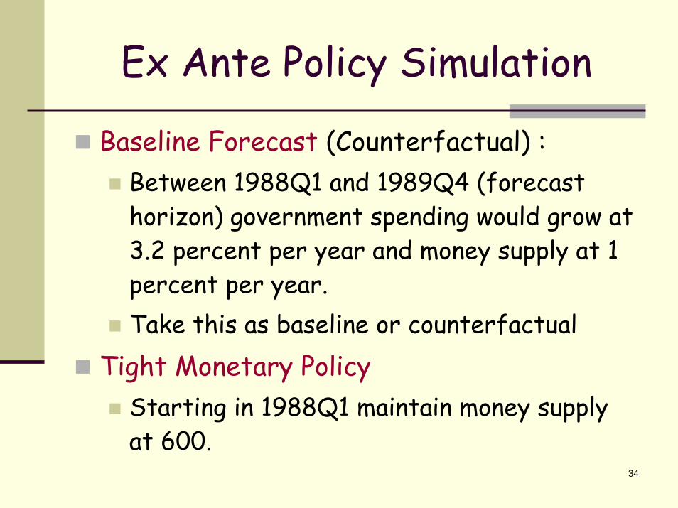
Baseline Forecast (Counterfactual) :Between 1988Q1 and 1989Q4 (forecast horizon) government spending would grow at 3.2 percent per year and money supply at 1 percent per year.Take this as baseline or counterfactual
Tight Monetary PolicyStarting in 1988Q1 maintain money supply at 600.
35
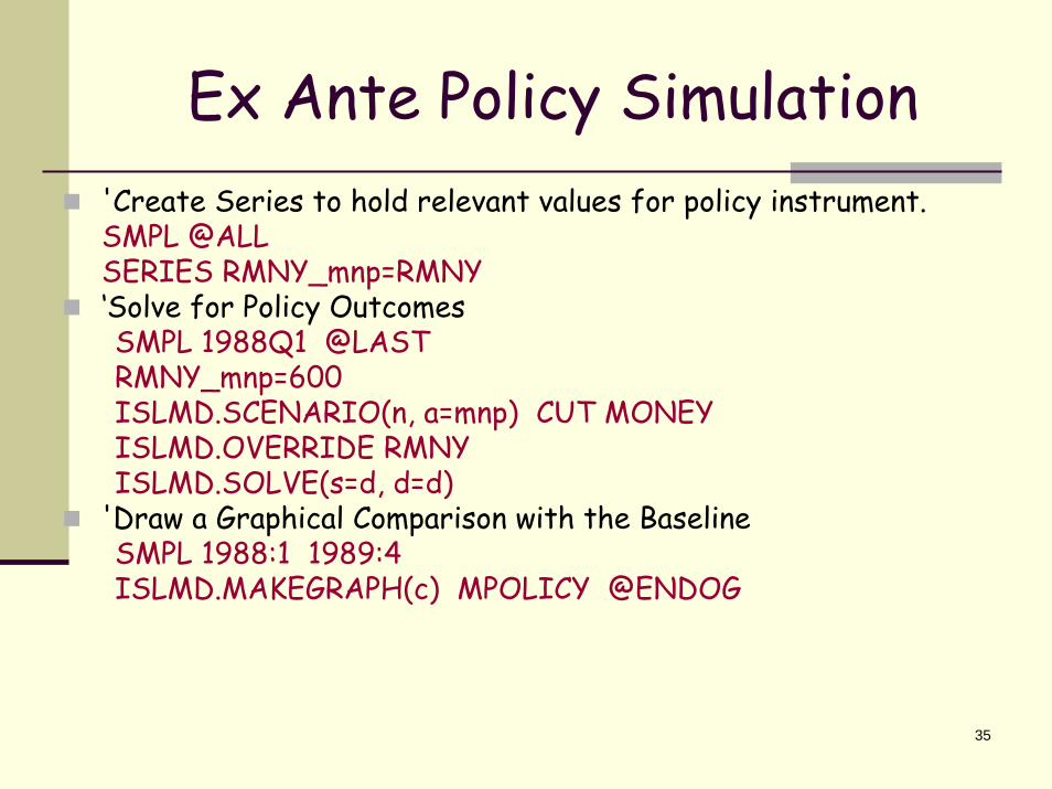
Ex Ante Policy Simulation'Create Series to hold relevant values for policy instrument.SMPL @ALLSERIES RMNY_mnp=RMNY‘Solve for Policy OutcomesSMPL 1988Q1 @LASTRMNY_mnp=600ISLMD.SCENARIO(n, a=mnp) CUT MONEYISLMD.OVERRIDE RMNYISLMD.SOLVE(s=d, d=d)
'Draw a Graphical Comparison with the BaselineSMPL 1988:1 1989:4ISLMD.MAKEGRAPH(c) MPOLICY @ENDOG

36
Tight Monetary Policy
2520
2560
2600
2640
2680
2720
88Q1 88Q2 88Q3 88Q4 89Q1 89Q2 89Q3 89Q4
Real Aggregate Personal Consumption (CUT MONEY)Real Aggregate Personal Consumption (Baseline)
Real Aggregate Personal Consumption
4000
4050
4100
4150
4200
4250
4300
88Q1 88Q2 88Q3 88Q4 89Q1 89Q2 89Q3 89Q4
Real GNP net of Exports and Imports (CUT MONEY)Real GNP net of Exports and Imports (Basel ine)
Real GNP net of Exports and Imports
720
730
740
750
760
88Q1 88Q2 88Q3 88Q4 89Q1 89Q2 89Q3 89Q4
Real Gross Domestic Investment (CUT MONEY)Real Gross Domestic Investment (Baseline)
Real Gross Domestic Investment
6
7
8
9
10
11
12
88Q1 88Q2 88Q3 88Q4 89Q1 89Q2 89Q3 89Q4
Interest Rate on Three-Month Treasury Bills (CUT MONEY)Interest Rate on Three-Month Treasury Bills (Baseline)
Interest Rate on Three-Month Treasury Bills

37
Tight Monetary PolicyA substantial increase in interest rate.Causes a sharp reduction in real gross domestic investment in 1989Q1. Real investment stays below the base path for the rest of the horizon.This leads to small reduction in GNP, and a very small decrease in real consumption.

38
Scenario Implementation
Definition: A set of assumptions about exogenous variables.Scenario implementation greatly facilitated by aliasing: Mapping of model variables into different sets of workfile series without having to alter equations of the model. This protects historical data from being overwritten
39
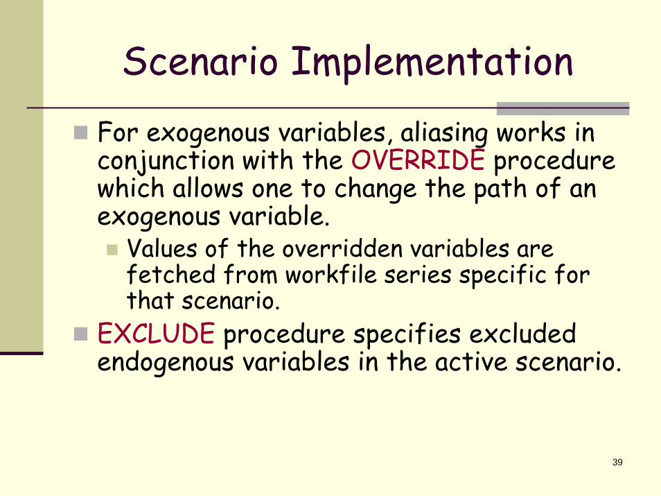
Scenario ImplementationFor exogenous variables, aliasing works in conjunction with the OVERRIDE procedure which allows one to change the path of an exogenous variable.
Values of the overridden variables are fetched from workfile series specific for that scenario.
EXCLUDE procedure specifies excluded endogenous variables in the active scenario.

40
Scenario ImplementationSolve Control for a Target
The CONTROL procedure solves for values on an exogenous variable so that a target endogenous variable follows a chosen trajectory.Syntax: model_name.control control_var target_var trajectoryExample: Control money supply so that GNP grows at 0.8 percent per quarter on average between 1987Q4 and 1989Q4.

41
Scenario ImplementationSMPL 1987Q4 1987Q4GNPTRAJ=GNPSMPL 1987Q4+1 @LAST
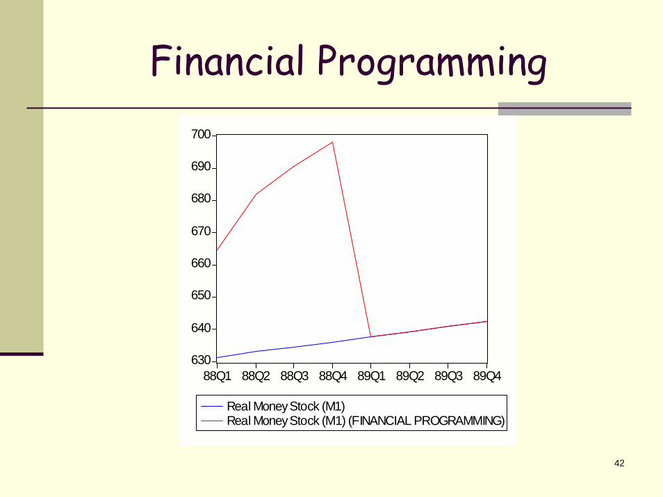
GNPTRAJ=(1+ (0.032/4))*GNPTRAJ(-1)SMPL 1988Q1 @LASTISLMD.SCENARIO(n, a=fpr) FINANCIAL PROGRAMMING ISLMD.OVERRIDE RMNYISLMD.CONTROL RMNY GNP GNPTRAJISLMD.SOLVE(s=d, d=d, c=1e-15)GROUP MSTOCK RMNY RMNY_fprFREEZE(MPROG) MSTOCK.LINEISLMD.MAKEGRAPH(c) FINANCIAL @ENDOG
42
Financial Programming
630
640
650
660
670
680
690
700
88Q1 88Q2 88Q3 88Q4 89Q1 89Q2 89Q3 89Q4
Real Money Stock (M1)Real Money Stock (M1) (FINANCIAL PROGRAMMING)

43
Financial Programming
2520
2560
2600
2640
2680
2720
88Q1 88Q2 88Q3 88Q4 89Q1 89Q2 89Q3 89Q4
Real Aggregate Personal Consumption (FINANCIAL PROGRAMMING)Real Aggregate Personal Consumption (Baseline)
Real Aggregate Personal Consumption
4000
4050
4100
4150
4200
4250
4300
88Q1 88Q2 88Q3 88Q4 89Q1 89Q2 89Q3 89Q4
Real GNP net of Exports and Imports (FINANCIAL PROGRAMMING)Real GNP net of Exports and Imports (Baseline)
Real GNP net of Exports and Imports
720
730
740
750
760
770
780
790
88Q1 88Q2 88Q3 88Q4 89Q1 89Q2 89Q3 89Q4
Real Gross Domestic Investment (FINANCIAL PROGRAMMING)Real Gross Domesti c Investment (Baseline)
Real Gross Domestic Investment
3
4
5
6
7
8
9
10
11
12
88Q1 88Q2 88Q3 88Q4 89Q1 89Q2 89Q3 89Q4
Interest Rate on Three-Month Treasury Bills (FINANCIAL PROGRAMMING)Interest Rate on Three-Month Treasury Bills (Baseline)
Interest Rate on Three-Month Treasury Bills

44
UpshotThe computation of the consequences of a policy choice is of vital importance in policy analysis.The model object in EViews provides a convenient tool for the job.Model specification relies on the MERGE or APPEND procedure depending on whether the equation is linked or inline.There are two basic solvers: Gauss-Seidel and Newton.The SCENARIO procedure greatly facilitates the implementation of various types of simulations:
Historical (validation)Ex post forecastEx ante forecast and policy simulations Solving the model in programming mode.

45
Exercise
Klein’s Model IStructureEstimationSimulation
46
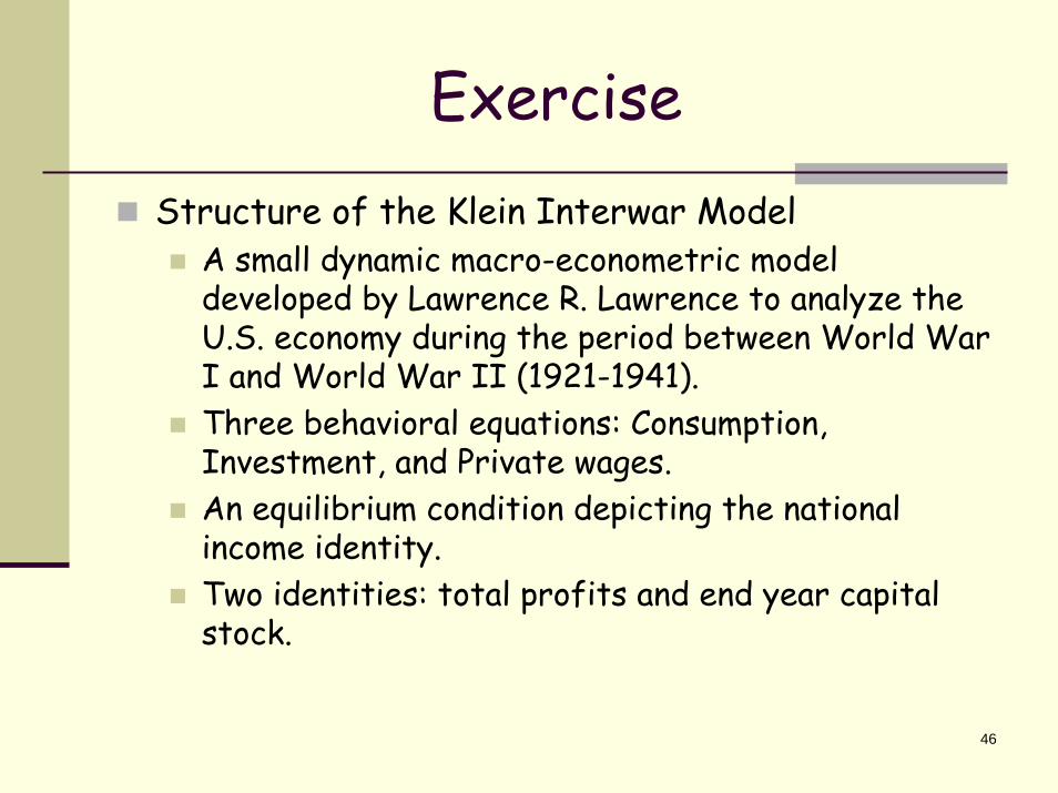
ExerciseStructure of the Klein Interwar Model
A small dynamic macro-econometric model developed by Lawrence R. Lawrence to analyze the U.S. economy during the period between World War I and World War II (1921-1941).Three behavioral equations: Consumption, Investment, and Private wages.An equilibrium condition depicting the national income identity.Two identities: total profits and end year capital stock.

47
ExerciseStructure of the Klein Interwar Model
Consumption
Net Investment
Private Wages
t
gt
ptttt WWPPC 141321 )( εαααα +++++= −
ttttt KPPI 2141321 εββββ ++++= −−
ttt
pt TimeXXW 341321 εγγγγ ++++= −

48
ExerciseStructure of the Klein Interwar Model
Goods Market Equilibrium
Profits
Capital Stock
tttt GICX ++=
ptttt WTXP −−=
ttt IKK += −1

49
ExerciseLimited and Full Information Estimation of Klein’s Model I.
Two-Stage Least SquaresUse equation object to find 2SLSEUse equation object and GMM command to 2SLSEUse system object to find 2SLSERecall Syntax:EQ_NAME.TSLS(OPTIONS) Y X1 [X2 X3 …] @Z1 [Z2 Z3 …]SYSTEM_NAME.TSLS(OPTIONS)EQ_NAME.GMM(OPTIONS) Y X1 [X2 X3 …] @Z1 [Z2 Z3 …]SYSTEM_NAME.GMM(OPTIONS)

50
Exercise
Limited and Full Information Estimation of Klein’s Model I.
GMM under HeteroskedasticityUse equation object and GMM command to produce estimates that are robust to unknown form of heteroskedasticity.
Three-Stage Least SquaresUse the system object to find 3SLSESyntax: SYSTEM_NAME.3SLS(OPTIONS)

51
Exercise
System: KLEIN2SLS Estimation Method: Two-Stage Least Squares Date: 10/10/05 Time: 15:54 Sample: 1921 1941 Included observations: 21 Total system (balanced) observations 63 Estimation settings: tol=0.00010, derivs=analytic (linear) Initial Values: ALPHA(1)=15.8295, ALPHA(2)=0.29304, ALPHA(3)=0.04782, ALPHA(4)=0.78180, BETA(1)=16.1710, BETA(2)=0.37981, BETA(3)=0.41245, BETA(4)=-0.14001, GAMMA(1)=2.08808, GAMMA(2)=0.37473, GAMMA(3)=0.20299, GAMMA(4)=0.18229
52
Exercise
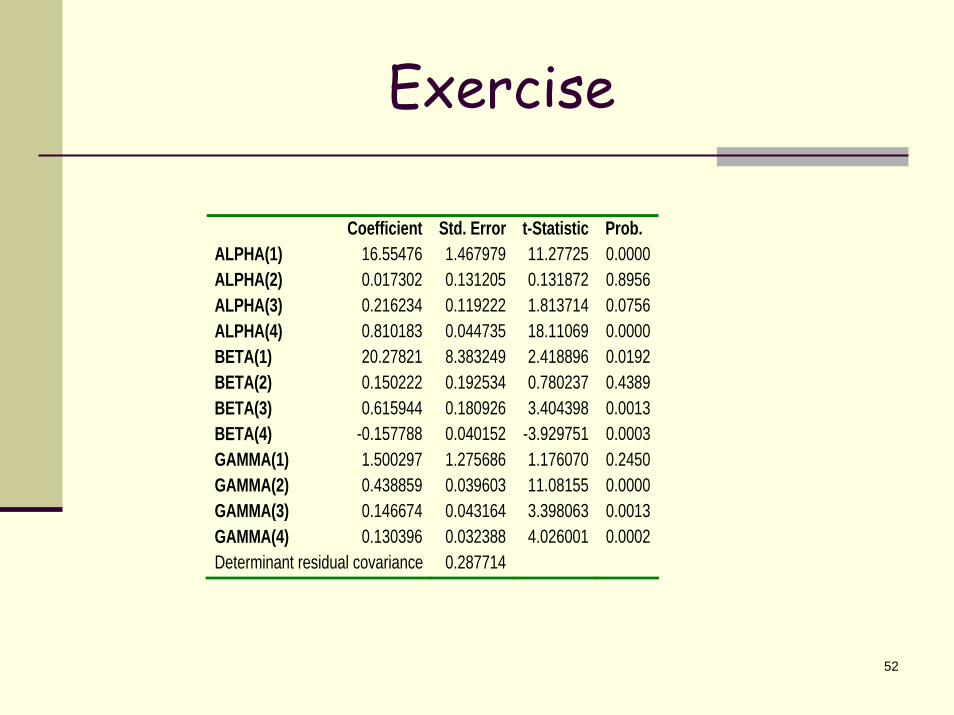
Coefficient Std. Error t-Statistic Prob. ALPHA(1) 16.55476 1.467979 11.27725 0.0000 ALPHA(2) 0.017302 0.131205 0.131872 0.8956 ALPHA(3) 0.216234 0.119222 1.813714 0.0756 ALPHA(4) 0.810183 0.044735 18.11069 0.0000 BETA(1) 20.27821 8.383249 2.418896 0.0192 BETA(2) 0.150222 0.192534 0.780237 0.4389 BETA(3) 0.615944 0.180926 3.404398 0.0013 BETA(4) -0.157788 0.040152 -3.929751 0.0003 GAMMA(1) 1.500297 1.275686 1.176070 0.2450 GAMMA(2) 0.438859 0.039603 11.08155 0.0000 GAMMA(3) 0.146674 0.043164 3.398063 0.0013 GAMMA(4) 0.130396 0.032388 4.026001 0.0002 Determinant residual covariance 0.287714

53
ExerciseEquation: CS=ALPHA(1) +ALPHA(2)*P +ALPHA(3)*P(-1)+ALPHA(4)*(WP+WG) Instruments: G T WG TIME K1 P(-1) X(-1) C Observations: 21 R-squared 0.976711 Mean dependent
var 53.99524
Adjusted R-squared 0.972601 S.D. dependent var 6.860866 S.E. of regression 1.135659 Sum squared resid 21.92525 Durbin-Watson stat 1.485072 Equation: I=BETA(1) +BETA(2)*P+BETA(3)*P(-1) +BETA(4)*K1 Instruments: G T WG TIME K1 P(-1) X(-1) C Observations: 21 R-squared 0.884884 Mean dependent
var 1.266667
Adjusted R-squared 0.864569 S.D. dependent var 3.551948 S.E. of regression 1.307149 Sum squared resid 29.04686 Durbin-Watson stat 2.085334 Equation: WP=GAMMA(1) +GAMMA(2)*X +GAMMA(3)*X(-1) +GAMMA(4)*TIME Instruments: G T WG TIME K1 P(-1) X(-1) C Observations: 21 R-squared 0.987414 Mean dependent
var 36.36190
Adjusted R-squared 0.985193 S.D. dependent var 6.304401 S.E. of regression 0.767155 Sum squared resid 10.00496 Durbin-Watson stat 1.963416
54
Exercise
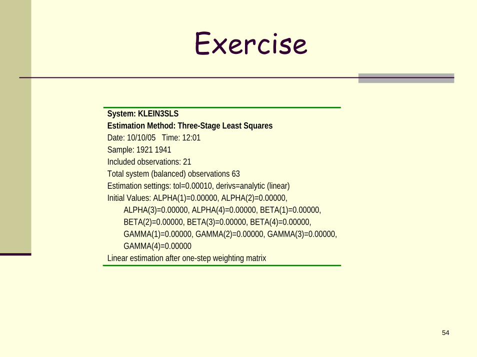
System: KLEIN3SLS Estimation Method: Three-Stage Least Squares Date: 10/10/05 Time: 12:01 Sample: 1921 1941 Included observations: 21 Total system (balanced) observations 63 Estimation settings: tol=0.00010, derivs=analytic (linear) Initial Values: ALPHA(1)=0.00000, ALPHA(2)=0.00000, ALPHA(3)=0.00000, ALPHA(4)=0.00000, BETA(1)=0.00000, BETA(2)=0.00000, BETA(3)=0.00000, BETA(4)=0.00000, GAMMA(1)=0.00000, GAMMA(2)=0.00000, GAMMA(3)=0.00000, GAMMA(4)=0.00000 Linear estimation after one-step weighting matrix

55
Exercise
Coefficient Std. Error t-Statistic Prob. ALPHA(1) 16.44079 1.304549 12.60266 0.0000 ALPHA(2) 0.124890 0.108129 1.155013 0.2535 ALPHA(3) 0.163144 0.100438 1.624323 0.1105 ALPHA(4) 0.790081 0.037938 20.82563 0.0000 BETA(1) 28.17785 6.793770 4.147601 0.0001 BETA(2) -0.013079 0.161896 -0.080787 0.9359 BETA(3) 0.755724 0.152933 4.941532 0.0000 BETA(4) -0.194848 0.032531 -5.989674 0.0000 GAMMA(1) 1.797218 1.115855 1.610619 0.1134 GAMMA(2) 0.400492 0.031813 12.58877 0.0000 GAMMA(3) 0.181291 0.034159 5.307304 0.0000 GAMMA(4) 0.149674 0.027935 5.357897 0.0000 Determinant residual covariance 0.282997

56
ExerciseEquation: CS=ALPHA(1) +ALPHA(2)*P +ALPHA(3)*P(-1)+ALPHA(4) *(WP+WG) Observations: 21 R-squared 0.980108 Mean dependent
var 53.99524
Adjusted R-squared 0.976598 S.D. dependent var 6.860866 S.E. of regression 1.049564 Sum squared resid 18.72696 Durbin-Watson stat 1.424939 Equation: I=BETA(1) +BETA(2)*P+BETA(3)*P(-1) +BETA(4)*K1 Observations: 21 R-squared 0.825805 Mean dependent
var 1.266667
Adjusted R-squared 0.795065 S.D. dependent var 3.551948 S.E. of regression 1.607958 Sum squared resid 43.95398 Durbin-Watson stat 1.995884 Equation: WP=GAMMA(1) +GAMMA(2)*X +GAMMA(3)*X(-1) +GAMMA(4)*TIME Observations: 21 R-squared 0.986262 Mean dependent
var 36.36190
Adjusted R-squared 0.983837 S.D. dependent var 6.304401 S.E. of regression 0.801490 Sum squared resid 10.92056 Durbin-Watson stat 2.155046
57
Exercise
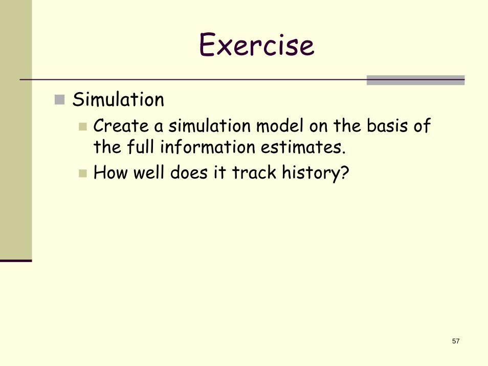
SimulationCreate a simulation model on the basis of the full information estimates.How well does it track history?

58
ReferencesBeals, Ralph E. 1972. Statistics for Economists: An Introduction. Chicago: Rand McNally& Co.Intriligator Michael D. 1978. Econometric Models, Techniques, and Applications. Englewood Cliffs: Prentice-Hall, Inc.Greene, William H. 2000. Econometric Analysis. Upper Saddle River: Prentice Hall.Hayashi, Fumio. 2000. Econometrics. Princeton: Princeton University Press.

59
ReferencesLanger, Susanne K. 1967. An Introduction to Symbolic Logic. New York. Dover Publications, Inc.Pindyck Robert S. and Rubinfeld Daniel L. 1998. Econometric Models and Economic Forecast (Fourth Edition). Boston: Irwin McGraw-Hill.Langer Susanne K. 1967. An Introduction to Symbolic Logic. New York: Dover Publications, Inc.Quantitative Micro Software (QMS). 2004. EViews 5.1 User’s Guide. Irvine : QMS

60
The End.