DEPARTMENT OF ECONOMICSUNIVERSITY OF CYPRUS

THE MM, ME, ML, EL, EF AND GMM APPROACHES TOESTIMATION: A SYNTHESIS

Anil K. Bera and Yannis Bilias

Discussion Paper 2001-09

P.O. Box 20537, 1678 Nicosia, CYPRUS Tel.: ++357-2-892430, Fax: ++357-2-892432Web site: http://www.econ.ucy.ac.cy

The MM, ME, ML, EL, EF and GMM Approaches to Estimation:

A Synthesis

Anil K. Bera∗

Department of Economics

University of Illinois

1206 S. 6th Street

Champaign, IL 61820; USA

Yannis Bilias

Department of Economics

University of Cyprus

P.O. Box 20537

1678 Nicosia; CYPRUS

JEL Classification: C13; C52

Keywords: Karl Pearson’s goodness-of-fit statistic; Entropy; Method of moment; Estimating

function; Likelihood; Empirical likelihood; Generalized method of moments; Power divergence

criterion; History of estimation.

∗Corresponding author: Anil K. Bera, Department of Economics, University of Illinois, Urbana-Champaign,

1206 S. 6th Street, Champaign, IL 61820, USA. Phone: (217) 333-4596; Fax: (217) 244-6678; email:

anil@fisher.econ.uiuc.edu

Abstract

The 20th century began on an auspicious statistical note with the publication of Karl

Pearson’s (1900) goodness-of-fit test, which is regarded as one of the most important scien-

tific breakthroughs. The basic motivation behind this test was to see whether an assumed

probability model adequately described the data at hand. Pearson (1894) also introduced

a formal approach to statistical estimation through his method of moments (MM) estima-

tion. Ronald A. Fisher, while he was a third year undergraduate at the Gonville and Caius

College, Cambridge, suggested the maximum likelihood estimation (MLE) procedure as

an alternative to Pearson’s MM approach. In 1922 Fisher published a monumental paper

that introduced such basic concepts as consistency, efficiency, sufficiency–and even the term

“parameter” with its present meaning. Fisher (1922) provided the analytical foundation

of MLE and studied its efficiency relative to the MM estimator. Fisher (1924a) established

the asymptotic equivalence of minimum χ2 and ML estimators and wrote in favor of using

minimum χ2 method rather than Pearson’s MM approach. Recently, econometricians have

found working under assumed likelihood functions restrictive, and have suggested using a

generalized version of Pearson’s MM approach, commonly known as the GMM estimation

procedure as advocated in Hansen (1982). Earlier, Godambe (1960) and Durbin (1960)

developed the estimating function (EF) approach to estimation that has been proven very

useful for many statistical models. A fundamental result is that score is the optimum EF.

Ferguson (1958) considered an approach very similar to GMM and showed that estimation

based on the Pearson chi-squared statistic is equivalent to efficient GMM. Golan, Judge

and Miller (1996) developed entropy-based formulation that allowed them to solve a wide

range of estimation and inference problems in econometrics. More recently, Imbens, Spady

and Johnson (1998), Kitamura and Stutzer (1997) and Mittelhammer, Judge and Miller

(2000) put GMM within the framework of empirical likelihood (EL) and maximum en-

tropy (ME) estimation. It can be shown that many of these estimation techniques can be

obtained as special cases of minimizing Cressie and Read (1984) power divergence crite-

rion that comes directly from the Pearson (1900) chi-squared statistic. In this way we are

able to assimilate a number of seemingly unrelated estimation techniques into a unified

framework.

1 Prologue: Karl Pearson’s method of moment estima-

tion and chi-squared test, and entropy

In this paper we are going to discuss various methods of estimation, especially those developed

in the twentieth century, beginning with a review of some developments in statistics at the

close of the nineteenth century. In 1892 W.F. Raphael Weldon, a zoologist turned statistician,

requested Karl Pearson (1857-1936) to analyze a set of data on crabs. After some investigation

Pearson realized that he could not fit the usual normal distribution to this data. By the early

1890’s Pearson had developed a class of distributions that later came to be known as the Pearson

system of curves, which is much broader than the normal distribution. However, for the crab data

Pearson’s own system of curves was not good enough. He dissected this “abnormal frequency

curve” into two normal curves as follows:

f(y) = αf1(y) + (1− α)f2(y), (1)

where

fj(y) =1√

2πσjexp[− 1

2σ2j

(y − µj)2], j = 1, 2.

This model has five parameters1 (α, µ1, σ21, µ2, σ

22). Previously, there had been no method avail-

able to estimate such a model. Pearson quite unceremoniously suggested a method that simply

equated the first five population moments to the respective sample counterparts. It was not

easy to solve five highly nonlinear equations. Therefore, Pearson took an analytical approach

of eliminating one parameter in each step. After considerable algebra he found a ninth-degree

polynomial equation in one unknown. Then, after solving this equation and by repeated back-

substitutions, he found solutions to the five parameters in terms of the first five sample moments.

It was around the autumn of 1893 he completed this work and it appeared in 1894. And this

was the beginning of the method of moment (MM) estimation. There is no general theory in

Pearson (1894). The paper is basically a worked-out “example” (though a very difficult one as

the first illustration of MM estimation) of a new estimation method.2

1The term “parameter” was introduced by Fisher (1922, p.311) [also see footnote 16]. Karl Pearson described

the “parameters” as “constants” of the “curve.” Fisher (1912) also used “frequency curve.” However, in Fisher

(1922) he used the term “distribution” throughout. “Probability density function” came much later, in Wilks

(1943, p.8) [see, David (1995)]2Shortly after Karl Pearson’s death, his son Egon Pearson provided an account of life and work of the elder

Pearson [see Pearson (1936)]. He summarized (pp.219-220) the contribution of Pearson (1894) stating, “The

paper is particularly noteworthy for its introduction of the method of moments as a means of fitting a theoretical

curve to observed data. This method is not claimed to be the best but is advocated from the utilitarian standpoint

1

After an experience of “some eight years” in applying the MM to a vast range of physical

and social data, Pearson (1902) provided some “theoretical” justification of his methodology.

Suppose we want to estimate the parameter vector θ = (θ1, θ2, . . . , θp)′ of the probability density

function f(y; θ). By a Taylor series expansion of f(y) ≡ f(y; θ) around y = 0, we can write

f(y) = φ0 + φ1y + φ2y2

2!+ φ3

y3

3!+ . . .+ φp

yp

p!+R, (2)

where φ0, φ1, φ2, . . . , φp depends on θ1, θ2, . . . , θp and R is the remainder term. Let f(y) be the

ordinate corresponding to y given by observations. Therefore, the problem is to fit a smooth

curve f(y; θ) to p histogram ordinates given by f(y). Then f(y) − f(y) denotes the distance

between the theoretical and observed curve at the point corresponding to y, and our objective

would be to make this distance as small as possible by a proper choice of φ0, φ1, φ2, . . . , φp [see

Pearson (1902, p.268)].3 Although Pearson discussed the fit of f(y) to p histogram ordinates

f(y), he proceeded to find a “theoretical” version of f(y) that minimizes [see Mensch (1980)]∫[f(y)− f(y)]2dy. (3)

Since f(.) is the variable, the resulting equation is∫[f(y)− f(y)]δfdy = 0, (4)

where, from (2), the differential δf can be written as

δf =

p∑j=0

(δφjyj

j!+∂R

∂φjδφj). (5)

Therefore, we can write equation (4) as∫[f(y)− f(y)]

p∑j=0

(δφjyj

j!+∂R

∂φjδφj)dy =

p∑j=0

∫[f(y)− f(y)](

yj

j!+∂R

∂φj)dyδφj = 0. (6)

Since the quantities φ0, φ1, φ2, . . . , φp are at our choice, for (6) to hold, each component should

be independently zero, i.e., we should have∫[f(y)− f(y)](

yj

j!+∂R

∂φj)dy = 0, j = 0, 1, 2, . . . , p, (7)

on the grounds that it appears to give excellent fits and provides algebraic solutions for calculating the constants

of the curve which are analytically possible.”3It is hard to trace the first use of smooth non-parametric density estimation in the statistics literature.

Koenker (2000, p.349) mentioned Galton’s (1885) illustration of “regression to the mean” where Galton averaged

the counts from the four adjacent squares to achieve smoothness. Karl Pearson’s minimization of the distance

between f(y) and f(y) looks remarkably modern in terms of ideas and could be viewed as a modern-equivalent

of smooth non-parametric density estimation [see also Mensch (1980)].

2

which is same as

µj = mj − j!∫

[f(y)− f(y)](∂R

∂φj)dy, j = 0, 1, 2, . . . , p. (8)

Here µj and mj are, respectively, the j-th moment corresponding to the theoretical curve f(y)

and the observed curve f(y).4 Pearson (1902) then ignored the integral terms arguing that they

involve the small factor f(y)− f(y), and the remainder term R, which by “hypothesis” is small

for large enough sample size. After neglecting the integral terms in (8), Pearson obtained the

equations

µj = mj, j = 0, 1, . . . , p. (9)

Then, he stated the principle of the MM as [see Pearson (1902, p.270)]: “To fit a good theoretical

curve f(y; θ1, θ2, . . . , θp) to an observed curve, express the area and moments of the curve for

the given range of observations in terms of θ1, θ2, . . . , θp, and equate these to the like quantities

for the observations.” Arguing that, if the first p moments of two curves are identical, the

higher moments of the curves becomes “ipso facto more and more nearly identical” for larger

sample size, he concluded that the “equality of moments gives a good method of fitting curves

to observations” [Pearson (1902, p.271)]. We should add that much of his theoretical argument

is not very rigorous, but the 1902 paper did provide a reasonable theoretical basis for the MM

and illustrated its usefulness.5 For detailed discussion on the properties of the MM estimator

see Shenton (1950, 1958, 1959).

After developing his system of curves [Pearson (1895)], Pearson and his associates were

fitting this system to a large number of data sets. Therefore, there was a need to formulate

a test to check whether an assumed probability model adequately explained the data at hand.

He succeeded in doing that and the result was Pearson’s celebrated (1900) χ2 goodness-of-

fit test. To describe the Pearson test let us consider a distribution with k classes with the

4It should be stressed that mj =∫yj f(y)dy =

∑ni y

ji πi with πi denoting the area of the bin of the ith

observation; this is not necessarily equal to the sample moment n−1∑i yji that is used in today’s MM. Rather,

Pearson’s formulation of empirical moments uses the efficient weighting πi under a multinomial probability

framework, an idea which is used in the literature of empirical likelihood and maximum entropy and to be

described later in this paper.5One of the first and possibly most important applications of MM idea is the derivation of t-distribution in

Student (1908) which was major breakthrough in introducing the concept of finite sample (exact) distribution in

statistics. Student (1908) obtained the first four moments of the sample variance S2, matched them with those of

the Pearson type III distribution, and concluded (p.4) “a curve of Professor Pearson’s type III may be expected

to fit the distribution of S2.” Student, however, was very cautious and quickly added (p.5), “it is probable that

the curve found represents the theoretical distribution of S2 so that although we have no actual proof we shall

assume it to do so in what follows.” And this was the basis of his derivation of the t-distribution. The name

t-distribution was given by Fisher (1924b).

3

probability of j-th class being qj(≥ 0), j = 1, 2, . . . , k and∑k

j=1 qj = 1. Suppose that according

to the assumed probability model, qj = qj0; therefore, one would be interested in testing the

hypothesis, H0 : qj = qj0, j = 1, 2, . . . , k. Let nj denote the observed frequency of the j-th

class, with∑k

j=1 nj = N. Pearson (1900) suggested the goodness-of-fit statistic6

P =k∑j=1

(nj −Nqj0)2

Nqj0=

k∑j=1

(Oj − Ej)2

Ej, (10)

where Oj and Ej denote, respectively, the observed and expected frequencies of the j-th class.

This is the first constructive test in the statistics literature. Broadly speaking, P is essentially

a distance measure between the observed and expected frequencies.

It is quite natural to question the relevance of this test statistic in the context of estimation.

Let us note that P could be used to measure the distance between any two sets of probabilities,

say, (pj, qj), j = 1, 2, . . . , k by simply writing pj = nj/N and qj = qj0, i.e.,

P = N

k∑j=1

(pj − qj)2

qj. (11)

As we will see shortly a simple transformation of P could generate a broad class of distance

measures. And later, in Section 5, we will demonstrate that many of the current estimation

procedures in econometrics can be cast in terms of minimizing the distance between two sets

of probabilities subject to certain constraints. In this way, we can tie and assimilate many

estimation techniques together using Pearson’s MM and χ2-statistic as the unifying themes.

We can write P as

P = N

k∑j=1

pj(pj − qj)qj

= N

k∑j=1

pj

(pjqj− 1

). (12)

Therefore, the essential quantity in measuring the divergence between two probability distribu-

tions is the ratio (pj/qj). Using Steven’s (1975) idea on “visual perception” Cressie and Read

6This test is regarded as one of the 20 most important scientific breakthroughs of this century along with

advances and discoveries like the theory of relativity, the IQ test, hybrid corn, antibiotics, television, the transistor

and the computer [see Hacking (1984)]. In his editorial in the inaugural issue of Sankhya, The Indian Journal of

Statistics, Mahalanobis (1933) wrote, “. . . the history of modern statistics may be said to have begun from Karl

Pearson’s work on the distribution of χ2 in 1900. The Chi-square test supplied for the first time a tool by which

the significance of the agreement or discrepancy between theoretical expectations and actual observations could

be judged with precision.” Even Pearson’s lifelong arch-rival Ronald A. Fisher (1922, p.314) conceded, “Nor

is the introduction of the Pearsonian system of frequency curves the only contribution which their author has

made to the solution of problems of specification: of even greater importance is the introduction of an objective

criterion of goodness of fit.” For more on this see Bera (2000) and Bera and Bilias (2001).

4

(1984) suggested using the relative difference between the perceived probabilities as (pj/qj)λ−1

where λ “typically lies in the range from 0.6 to 0.9” but could theoretically be any real num-

ber [see also Read and Cressie (1988, p.17)]. By weighing this quantity proportional to pj and

summing over all the classes, leads to the following measure of divergence:

k∑j=1

pj

[(pjqj

)λ− 1

]. (13)

This is approximately proportional to the Cressie and Read (1984) power divergence family of

statistics7

Iλ(p, q) =2

λ(λ+ 1)

k∑j=1

pj

[(pjqj

)λ− 1

]

=2

λ(λ+ 1)

k∑j=1

qj

[{1 +

(pjqj− 1

)}λ+1

− 1

], (14)

where p = (p1, p2, . . . , pn)′ and q = (q1, q2, . . . , qn)′. Lindsay (1994, p.1085) calls δj = (pj/qj)− 1

the “Pearson” residual since we can express the Pearson statistic in (11) as P = N∑k

j=1 qjδ2j .

From this, it is immediately seen that when λ = 1, Iλ(p, q) reduces to P/N . In fact, a number

of well-known test statistics can be obtained from Iλ(p, q). When λ→ 0, we have the likelihood

(LR) test statistic, which, as an alternative to (10), can be written as

LR = 2k∑j=1

nj ln

(njNqj0

)= 2

k∑j=1

Oj ln

(Oj

Ej

). (15)

Similarly, λ = −1/2 gives the Freeman and Tukey (FT) (1950) statistic, or Hellinger distance,

FT = 4k∑j=1

(√nj −

√nqj0)2 = 4

k∑j=1

(√Oj −

√Ej)

2. (16)

All these test statistics are just different measures of distance between the observed and expected

frequencies. Therefore, Iλ(p, q) provides a very rich class of divergence measures.

Any probability distribution pi, i = 1, 2, . . . , n (say) of a random variable taking n values

provides a measure of uncertainty regarding that random variable. In the information theory

literature, this measure of uncertainty is called entropy. The origin of the term “entropy” goes

7In the entropy literature this is known as Renyi’s (1961) α-class generalized measures of entropy [see Maa-

soumi (1993, p.144), Ullah (1996, p.142) and Mittelhammer, Judge and Miller (2000, p.328)]. Golan, Judge and

Miller (1996, p.36) referred to Schutzenberger (1954) as well. This formulation has also been used extensively

as a general class of decomposable income inequality measures, for example, see Cowell (1980) and Shorrocks

(1980), and in time-series analysis to distinguish chaotic data from random data [Pompe (1994)].

5

back to thermodynamics. The second law of thermodynamics states that there is an inherent

tendency for disorder to increase. A probability distribution gives us a measure of disorder.

Entropy is generally taken as a measure of expected information, that is, how much information

do we have in the probability distribution pi, i = 1, 2, . . . , n. Intuitively, information should be

a decreasing function of pi, i.e., the more unlikely an event, the more interesting it is to know

that it can happen [see Shannon and Weaver (1949, p.105) and Sen (1975, pp.34-35)].

A simple choice for such a function is − ln pi. Entropy H(p) is defined as a weighted sum of

the information − ln pi, i = 1, 2, . . . , n with respective probabilities as weights, namely,

H(p) = −∑

pi ln pi. (17)

If pi = 0 for some i, then pi ln pi is taken to be zero. When pi = 1/n for all i, H(p) = lnn

and then we have the maximum value of the entropy and consequently the least information

available from the probability distribution. The other extreme case occurs when pi = 1 for one

i, and = 0 for the rest; then H(p) = 0. If we do not weigh each − ln pi by pi and simply take

the sum, another measure of entropy would be

H ′(p) = −n∑i=1

ln pi. (18)

Following (17), the cross-entropy of one probability distribution p = (p1, p2, . . . , pn)′ with respect

to another distribution q = (q1, q2, . . . , qn)′ can be defined as

C(p, q) =n∑i=1

pi ln(pi/qi) = E[ln p]− E[ln q], (19)

which is yet another measure of distance between two distributions. It is easy to see the link

between C(p, q) and the Cressie and Read (1984) power divergence family. If we choose q =

(1/n, 1/n, . . . , 1/n)′ = i/n where i is a n× 1 vector of ones, C(p, q) reduces to

C(p, i/n) =n∑i=1

pi ln pi − lnn. (20)

Therefore, entropy maximization is a special case of cross-entropy minimization with respect to

the uniform distribution. For more on entropy, cross-entropy and their uses in econometrics see

Maasoumi (1993), Ullah (1996), Golan, Judge and Miller (1996, 1997 and 1998), Zellner and

Highfield (1988), Zellner (1991) and other papers in Grandy and Schick (1991), Zellner (1997)

and Mittelhammer, Judge and Miller (2000).

If we try to find a probability distribution that maximizes the entropy H(p) in (17), the

optimal solution is the uniform distribution, i.e., p∗ = i/n. In the Bayesian literature, it is

6

common to maximize an entropy measure to find non-informative priors. Jaynes (1957) was

the first to consider the problem of finding a prior distribution that maximizes H(p) subject to

certain side conditions, which could be given in the form of some moment restrictions. Jaynes’

problem can be stated as follows. Suppose we want to find a least informative probability

distribution pi = Pr(Y = yi), i = 1, 2, . . . , n of a random variable Y satisfying, say, m moment

restrictions E[hj(Y )] = µj with known µj’s, j = 1, 2, . . . ,m. Jaynes (1957, p.623) found an

explicit solution to the problem of maximizing H(p) subject to the above moment conditions

and∑n

i=1 pi = 1 [for a treatment of this problem under very general conditions, see, Haberman

(1984)]. We can always find some (in fact, many) solutions just by satisfying the constraints;

however, maximization of (17) makes the resulting probabilities pi (i = 1, 2, . . . , n) as smooth

as possible. Jaynes (1957) formulation has been extensively used in the Bayesian literature

to find priors that are as noninformative as possible given some prior partial information [see

Berger (1985, pp.90-94)]. In recent years econometricians have tried to estimate parameter(s) of

interest say, θ, utilizing only certain moment conditions satisfied by the underlying probability

distribution, known as the generalized method of moments (GMM) estimation. The GMM

procedure is an extension of Pearson’s (1895, 1902) MM when we have more moment restrictions

than the dimension of the unknown parameter vector. The GMM estimation technique can

also be cast into the information theoretic approach of maximization of entropy following the

empirical likelihood (EL) method of Owen (1988, 1990, 1991) and Qin and Lawless (1994).

Back and Brown (1993), Kitamura and Stutzer (1997) and Imbens, Spady and Johnson (1998)

developed information theoretic approaches of entropy maximization estimation procedures that

include GMM as a special case. Therefore, we observe how seemingly distinct ideas of Pearson’s

χ2 test statistic and GMM estimation are tied to the common principle of measuring distance

between two probability distributions through the entropy measure. The modest aim of this

review paper is essentially this idea of assimilating distinct estimation methods. In the following

two sections we discuss Fisher’s (1912, 1922) maximum likelihood estimation (MLE) approach

and its relative efficiency to the MM estimation method. The MLE is the forerunner of the

currently popular EL approach. We also discuss the minimum χ2 method of estimation, which

is based on the minimization of the Pearson χ2 statistic. Section 4 proceeds with optimal

estimation using an estimating function (EF) approach. In Section 5, we discuss the instrumental

variable (IV) and GMM estimation procedure along with their recent variants. Both EF and

GMM approaches were devised in order to handle problems of method of moments estimation

where the number of moment restrictions is larger than the number of parameters. The last

section provides some concluding remarks. While doing the survey, we also try to provide some

personal perspectives on researchers who contributed to the amazing progress in statistical and

7

econometrics estimation techniques that we have witnessed in the last 100 years. We do this

since in many instances the original motivation and philosophy of various statistical techniques

have become clouded over time. And to the best of our knowledge these materials have not

found a place in econometric textbooks.

2 Fisher’s (1912) maximum likelihood, and the minimum

chi-squared methods of estimation

In 1912 when R. A. Fisher published his first mathematical paper, he was a third and final

year undergraduate in mathematics and mathematical physics in Gonville and Caius College,

Cambridge. It is now hard to envision exactly what prompted Fisher to write this paper.

Possibly, his tutor the astronomer F. J. M. Stratton (1881-1960), who lectured on the theory of

errors, was the instrumental factor. About Stratton’s role, Edwards (1997a, p.36) wrote: “In the

Easter Term 1911 he had lectured at the observatory on Calculation of Orbits from Observations,

and during the next academic year on Combination of Observations in the Michaelmas Term

(1911), the first term of Fisher’s third and final undergraduate year. It is very likely that Fisher

attended Stratton’s lectures and subsequently discussed statistical questions with him during

mathematics supervision in College, and he wrote the 1912 paper as a result.”8

The paper started with a criticism of two known methods of curve fitting, least squares and

Pearson’s MM. In particular, regarding MM, Fisher (1912, p.156) stated “a choice has been

made without theoretical justification in selecting r equations . . . ” Fisher was referring to the

equations in (9), though Pearson (1902) defended his choice on the ground that these lower-order

moments have smallest relative variance [see Hald (1998, p.708)].

After disposing of these two methods, Fisher stated “we may solve the real problem directly”

and set out to discuss his absolute criterion for fitting frequency curves. He took the probability

density function (p.d.f) f(y; θ) (using our notation) as an ordinate of the theoretical curve of

unit area and, hence, interpreted f(y; θ)δy as the chance of an observation falling within the

8Fisher (1912) ends with “In conclusion I should like to acknowledge the great kindness of Mr. J.F.M. Stratton,

to whose criticism and encouragement the present form of this note is due.” It may not be out of place to add

that in 1912 Stratton also prodded his young pupil to write directly to Student (William S. Gosset, 1876-1937),

and Fisher sent Gosset a rigorous proof of t-distribution. Gosset was sufficiently impressed to send the proof

to Karl Pearson with a covering letter urging him to publish it in Biometrika as a note. Pearson, however, was

not impressed and nothing more was heard of Fisher’s proof [see Box (1978, pp.71-73) and Lehmann (1999,

pp.419-420)]. This correspondence between Fisher and Gosset was the beginning of a lifelong mutual respect

and friendship until the death of Gosset.

8

range δy. Then he defined (p.156)

lnP ′ =n∑i=1

ln f(yi; θ)δyi (21)

and interpreted P ′ to be “proportional to the chance of a given set of observations occurring.”

Since the factors δyi are independent of f(y; θ), he stated that the “probability of any particular

set of θ’s is proportional to P ,” where

lnP =n∑i=1

ln f(yi; θ) (22)

and the most probable set of values for the θ’s will make P a maximum” (p.157). This is in

essence Fisher’s idea regarding maximum likelihood estimation.9 After outlining his method for

fitting curves, Fisher applied his criterion to estimate parameters of a normal density of the

following form

f(y;µ, h) =h√π

exp[−h2(y − µ)2], (23)

where h = 1/σ√

2 in the standard notation of N(µ, σ2). He obtained the “most probable values”

as10

µ =1

n

n∑i=1

yi (24)

and

h2 =n

2∑n

i=1(yi − y)2. (25)

Fisher’s probable value of h did not match the conventional value that used (n − 1) rather

than n as in (25) [see Bennett (1907-1908)]. By integrating out µ from (23), Fisher obtained

9We should note that nowhere in Fisher (1912) he uses the word “likelihood.” It came much later in Fisher

(1921, p.24), and the phrase “method of maximum likelihood” was first used in Fisher (1922, p.323) [also see

Edwards (1997a, p.36)]. Fisher (1912) did not refer to the Edgeworth (1908, 1909) inverse probability method

which gives the same estimates, or for that matter to most of the early literature (the paper contained only two

references). As Aldrich (1997, p.162) indicated “nobody” noticed Edgeworth work until “Fisher had redone it.”

Le Cam (1990, p.153) settled the debate on who first proposed the maximum likelihood method in the following

way: “Opinions on who was the first to propose the method differ. However Fisher is usually credited with

the invention of the name ‘maximum likelihood’, with a major effort intended to spread its use and with the

derivation of the optimality properties of the resulting estimates.” We can safely say that although the method

of maximum likelihood pre-figured in earlier works, it was first presented in its own right, and with a full view

of its significance by Fisher (1912) and later by Fisher (1922).10In fact Fisher did not use notations µ and h. Like Karl Pearson he did not distinguish between the parameter

and its estimator. That came much later in Fisher (1922, p.313) when he introduced the concept of “statistic.”

9

the “variation of h,” and then maximizing the resulting marginal density with respect to h, he

found the conventional estimator

ˆh

2

=n− 1

2∑n

i=1(yi − y)2. (26)

Fisher (p.160) interpreted

P =n∏i=1

f(yi; θ) (27)

as the “relative probability of the set of values” θ1, θ2, . . . , θp. Implicitly, he was basing his

arguments on inverse probability (posterior distribution) with noninformative prior. But at the

same time he criticized the process of obtaining (26) saying “integration” with respect to µ is

“illegitimate and has no meaning with respect to inverse probability.” Here Fisher’s message is

very confusing and hard to decipher.11 In spite of these misgivings Fisher (1912) is a remarkable

paper given that it was written when Fisher was still an undergraduate. In fact, his idea of

the likelihood function (27) played a central role in introducing and crystallizing some of the

fundamental concepts in statistics.

The history of the minimum chi-squared (χ2) method of estimation is even more blurred.

Karl Pearson and his associates routinely used the MM to estimate parameters and the χ2

statistic (10) to test the adequacy of the fitted model. This state of affairs prompted Hald

(1998, p.712) to comment: “One may wonder why he [Karl Pearson] did not take further step

to minimizing χ2 for estimating the parameters.” In fact, for a while, nobody took a concrete

step in that direction. As discussed in Edwards (1997a) several early papers that advocated

this method of estimation could be mentioned: Harris (1912), Engledow and Yule (1914), Smith

(1916) and Haldane (1919a, b). Ironically, it was the Fisher (1928) book and its subsequent

editions that brought to prominence this estimation procedure. Smith (1916) was probably the

first to state explicitly how to obtain parameter estimates using the minimum χ2 method. She

started with a mild criticism of Pearson’s MM (p.11): “It is an undoubtedly utile and accurate

method; but the question of whether it gives the ‘best’ values of the constant has not been

very fully studied.”12 Then, without much fanfare she stated (p.12): “From another standpoint,

11In Fisher (1922, p.326) he went further and confessed: “I must indeed plead guilty in my original statement

in the Method of Maximum Likelihood [Fisher (1912)] to having based my argument upon the principle of inverse

probability; in the same paper, it is true, I emphasized the fact that such inverse probabilities were relative only.”

Aldrich (1997), Edwards (1997b) and Hald (1999) examined Fisher’s paradoxical views to “inverse probability”

in detail.12Kirstine Smith was a graduate student in Karl Pearson’s laboratory since 1915. In fact her paper ends with

the following acknowledgement: “The present paper was worked out in the Biometric Laboratory and I have to

thank Professor Pearson for his aid throughout the work.” It is quite understandable that she could not be too

critical of Pearson’s MM.

10

however, the ‘best values’ of the frequency constants may be said to be those for which” the

quantity in (10) “is a minimum.” She argued that when χ2 is a minimum, “the probability of

occurrence of a result as divergent as or more divergent than the observed, will be maximum.”

In other words, using the minimum χ2 method the “goodness-of-fit” might be better than that

obtained from the MM. Using a slightly different notation let us express (10) as

χ2(θ) =k∑j=1

[nj −Nqj(θ)]2

Nqj(θ), (28)

where Nqj(θ) is the expected frequency of the j-th class with θ = (θ1, θ2, . . . , θp)′ as the unknown

parameter vector. We can write

χ2(θ) =k∑j=1

n2j

Nqj(θ)−N. (29)

Therefore, the minimum χ2 estimates will be obtained by solving ∂χ2(θ)/∂θ = 0, i.e., from

k∑j=1

n2j

[Nqj(θ)]2∂qj(θ)

∂θl= 0, l = 1, 2, . . . , p. (30)

This is Smith’s (1916, p.264) system of equations (1). Since “these equations will generally be

far too involved to be directly solved” she approximated these around MM estimates. Without

going in that direction let us connect these equations to those from Fisher’s (1912) ML equations.

Since∑k

j=1 qj(θ) = 1, we have∑k

j=1 ∂qj(θ)/∂θl = 0, and hence from (30), the minimum χ2

estimating equations are

k∑j=1

n2j − [Nqj(θ)]

2

[Nqj(θ)]2∂qj(θ)

∂θl= 0, l = 1, 2, . . . , p. (31)

Under the multinomial framework, Fisher’s likelihood function (27), denoted as L(θ) is

L(θ) = N !k∏j=1

[(nj)−1]

k∏j=1

[qj(θ)]nj . (32)

Therefore, the log-likelihood function (22), denoted by `(θ), can be written as

lnL(θ) = `(θ) = constant +k∑j=1

nj ln qj(θ). (33)

The corresponding ML estimating equations are ∂`(θ)/∂θ = 0, i.e.,

k∑j=1

njqj(θ)

∂qj(θ)

∂θl= 0, (34)

11

i.e.,k∑j=1

[nj −Nqj(θ)]Nqj(θ)

· ∂qj(θ)∂θl

= 0, l = 1, 2, . . . , p. (35)

Fisher (1924a) argued that the difference between (31) and (35) is of the factor [nj+Nqj(θ)]/Nqj(θ),

which tends to value 2 for large values of N , and therefore, these two methods are asymptotically

equivalent.13 Some of Smith’s (1916) numerical illustration showed improvement over MM in

terms of goodness-of-fit values (in her notation P ) when minimum χ2 method was used. How-

ever, in her conclusion to the paper Smith (1916) provided a very lukewarm support for the

minimum χ2 method.14 It is, therefore, not surprising that this method remained dormant for

a while even after Neyman and Pearson (1928, pp.265-267) provided further theoretical justi-

fication. Neyman (1949) provided a comprehensive treatment of χ2 method of estimation and

testing. Berkson (1980) revived the old debate, questioned the sovereignty of MLE and argued

that minimum χ2 is the primary principle of estimation. However, the MLE procedure still

remains as one of the most important principles of estimation and Fisher’s idea of the likelihood

plays the fundamental role in it. It can be said that based on his 1912 paper, Ronald Fisher

was able to contemplate much broader problems later in his research that eventually culminated

in his monumental paper in 1922. Because of the enormous importance of Fisher (1922) in the

history of estimation, in the next section we provide a critical and detail analysis of this paper.

13Note that to compare estimates from two different methods Fisher (1924a) used the “estimating equations”

rather than the estimates. Using the estimating equations (31) Fisher (1924a) also showed that χ2(θ) has k−p−1

degrees of freedom instead of k − 1 when the p× 1 parameter vector θ is replaced by its estimator θ. In Section

4 we will discuss the important role estimating equations play.14Part of her concluding remarks was “. . . the present numerical illustrations appear to indicate that but little

practical advantage is gained by a great deal of additional labour, the values of P are only slightly raised–probably

always within their range of probable error. In other words the investigation justifies the method of moments as

giving excellent values of the constants with nearly the maximum value of P or it justifies the use of the method

of moments, if the definition of ‘best’ by which that method is reached must at least be considered somewhat

arbitrary.” Given that the time when MM was at its highest of popularity and Smith’s position under Pearson’s

laboratory, it was difficult for her to make a strong recommendation for minimum χ2 method [see also footnote

12].

12

3 Fisher’s (1922) mathematical foundations of theoreti-

cal statistics and further analysis on MM and ML es-

timation

If we had to name the single most important paper on the theoretical foundation of statisti-

cal estimation theory, we could safely mention Fisher (1922).15 The ideas of this paper are

simply revolutionary. It introduced many of the fundamental concepts in estimation, such as,

consistency, efficiency, sufficiency, information, likelihood and even the term “parameter” with

its present meaning [see Stephen Stigler’s comment on Savage (1976)].16 Hald (1998, p.713)

succinctly summarized the paper by saying: “For the first time in the history of statistics a

framework for a frequency-based general theory of parametric statistical inference was clearly

formulated.”

In this paper (p.313) Fisher divided the statistical problems into three clear types:

“(1) Problems of Specification. These arise in the choice of the mathematical form

of the population.

(2) Problems of Estimation. These involve the choice of methods of calculating from

a sample statistical derivates, or as we shall call them statistics, which are designed

to estimate the values of the parameters of the hypothetical population.

(3) Problems of Distribution. These include discussions of the distribution of statis-

tics derived from samples, or in general any functions of quantities whose distribution

is known.”

Formulation of the general statistical problems into these three broad categories was not

really entirely new. Pearson (1902, p.266) mentioned the problems of (a) “choice of a suitable

curve”, (b) “determination of the constants” of the curve, “when the form of the curve has

15The intervening period between Fisher’s 1912 and 1922 papers represented years in wilderness for Ronald

Fisher. He contemplated and tried many different things, including joining the army and farming, but failed.

However, by 1922, Fisher has attained the position of Chief Statistician at the Rothamsted Experimental Station.

For more on this see Box (1978, ch.2) and Bera and Bilias (2000).16Stigler (1976, p.498) commented that, “The point is that it is to Fisher that we owe the introduction of

parametric statistical inference (and thus nonparametric inference). While there are other interpretations under

which this statement can be defended, I mean it literally–Fisher was principally responsible for the introduction

of the word “parameter” into present statistical terminology!” Stigler (1976, p.499) concluded his comment by

saying “. . . for a measure of Fisher’s influence on our field we need look no further than the latest issue of any

statistical journal, and notice the ubiquitous “parameter.” Fisher’s concepts so permeate modern statistics, that

we tend to overlook one of the most fundamental!”

13

been selected” and finally, (c) measuring the goodness-of-fit. Pearson had ready solutions for

all three problems, namely, Pearson’s family of distributions, MM and the test statistic (10), for

(a), (b) and (c), respectively. As Neyman (1967, p.1457) indicated, Emile Borel also mentioned

these three categories in his book, Elements de la Theorie des Probabilities, 1909. Fisher (1922)

did not dwell on the problem of specification and rather concentrated on the second and third

problems, as he declared (p.315): “The discussion of theoretical statistics may be regarded as

alternating between problems of estimation and problems of distribution.”

After some general remarks about the then-current state of theoretical statistics, Fisher

moved on to discuss some concrete criteria of estimation, such as, consistency, efficiency and

sufficiency. Of these three, Fisher (1922) found the concept of “sufficiency” the most powerful

to advance his ideas on the ML estimation. He defined “sufficiency” as (p.310): “A statistic

satisfies the criterion of sufficiency when no other statistic which can be calculated from the same

sample provides any additional information as to the value of the parameter to be estimated.”

Let t1 be sufficient for θ and t2 be any other statistic, then according to Fisher’s definition

f(t1, t2; θ) = f(t1; θ)f(t2|t1), (36)

where f(t2|t1) does not depend on θ. Fisher further assumed that t1 and t2 asymptotically follow

bivariate normal (BN) distribution as(t1

t2

)∼ BN

[(θ

θ

),

(σ2

1 ρσ1σ2

ρσ1σ2 σ22

)], (37)

where −1 < ρ < 1 is correlation coefficient. Therefore,

E(t2|t1) = θ + ρσ2

σ1

(t1 − θ) and V (t2|t1) = σ22(1− ρ2). (38)

Since t1 is sufficient for θ, the distribution of t2|t1 should be free of θ and we should have ρσ2

σ1= 1

i.e., σ21 = ρ2σ2

2 ≤ σ22. In other words, the sufficient statistic t1 is “efficient” [also see Geisser

(1980, p.61), and Hald (1998, p.715)]. One of Fisher’s aim was to establish that his MLE has

minimum variance in large samples.

To demonstrate that the MLE has minimum variance, Fisher relied on two main steps. The

first, as stated earlier, is that a “sufficient statistic” has the smallest variance. And for the

second, Fisher (1922, p.330) showed that “the criterion of sufficiency is generally satisfied by the

solution obtained by method of maximum likelihood . . . ” Without resorting to the central limit

theorem, Fisher (1922, pp.327-329) proved the asymptotic normality of the MLE. For details

on Fisher’s proofs see Bera and Bilias (2000). However, Fisher’s proofs are not satisfactory. He

himself realized that and confessed (p.323): “I am not satisfied as to the mathematical rigour

14

of any proof which I can put forward to that effect. Readers of the ensuing pages are invited to

form their own opinion as to the possibility of the method of the maximum likelihood leading in

any case to an insufficient statistic. For my own part I should gladly have withheld publication

until a rigorously complete proof could have been formulated; but the number and variety of

the new results which the method discloses press for publication, and at the same time I am

not insensible of the advantage which accrues to Applied Mathematics from the co-operation

of the Pure Mathematician, and this co-operation is not infrequently called forth by the very

imperfections of writers on Applied Mathematics.”

A substantial part of Fisher (1922) is devoted to the comparison of ML and MM estimates

and establishing the former’s superiority (pp.321-322, 332-337, 342-356), which he did mainly

through examples. One of his favorite examples is the Cauchy distribution with density function

f(h; θ) =1

π

1

[1 + (y − θ)2], −∞ < y <∞. (39)

The problem is to estimate θ given a sample y = (y1, y2, . . . , yn)′. Fisher (1922, p.322) stated:

“By the method of moments, this should be given by the first moment, that is by the mean

of the observations: such would seem to be at least a good estimate. It is, however, entirely

valueless. The distribution of the mean of such samples is in fact the same, identically, as that

of a single observations.” However, this is an unfair comparison. Since no moments exist for

the Cauchy distribution, Pearson’s MM procedure is just not applicable here.

Fisher (1922) performed an extensive analysis of the efficiency of ML and MM estimators

for fitting distributions belonging to the Pearson (1895) family. Fisher (1922, p.355) concluded

that the MM has an efficiency exceeding 80 percent only in the restricted region for which the

kurtosis coefficient lies between 2.65 and 3.42 and the skewness measure does not exceed 0.1.

In other words, only in the immediate neighborhood of the normal distribution, the MM will

have high efficiency.17 Fisher (1922, p.356) characterized the class of distributions for which the

MM and ML estimators will be approximately the same in a simple and elegant way. The two

17Karl Pearson responded to Fisher’s criticism of MM and other related issues in one of his very last papers,

Pearson (1936), that opened with the italicized and striking line: “Wasting your time fitting curves by moments,

eh?” Fisher felt compelled to give a frank reply immediately but waited until Pearson died in 1936. Fisher

(1937, p.303) wrote in the opening section of his paper “. . . The question he [Pearson] raised seems to me not at

all premature, but rather overdue.” After his step by step rebutal to Pearson’s (1936) arguments, Fisher (1937,

p.317) placed Pearson’s MM approach in statistical teaching as: “So long as ‘fitting curves by moments’ stands in

the way of students’ obtaining proper experience of these other activities, all of which require time and practice,

so long will it be judged with increasing confidence to be waste of time.” For more on this see Box (1978,

pp.329-331). Possibly this was the temporary death nail for the MM. But after half a century, econometricians

are finding that Pearson’s moment matching approach to estimation is more useful than Fisher’s ML method of

estimation.

15

estimators will be identical if the derivative of the log-likelihood function has the following form

∂`(θ)

∂θ= a0 + a1

n∑i=1

yi + a2

n∑i=1

y2i + a3

n∑i=1

y3i + a4

n∑i=1

y4i + . . . . . . (40)

Therefore, we should be able to write the density of Y as18

f(y) ≡ f(y; θ) = C exp[b0 + b1y + b2y2 + b3y

3 + b4y4] (41)

(keeping terms up to order 4), where bj(j = 0, 1, . . . , 4) depend on θ and the constant C is such

that the total probability is 1. Without any loss of generality, let us take b1 = 0, then we have

d ln f(y)

dy= 2b2y + 3b3y

2 + 4b4y3

= 2b2y

(1 +

3b3y

2b2

+2b4y

2

b2

). (42)

If b3 and b4 are small, i.e., when the density is sufficiently near to the normal curve, we can write

(42) approximately as

d ln f(y)

dy= 2b2y

(1− 3b3y

2b2

− 2b4y2

b2

)−1

. (43)

The form (43) corresponds to the Pearson (1895) general family of distributions. Therefore, the

MM will have high efficiency within the class of Pearson family of distributions only when the

density is close to the normal curve.

However, the optimality properties of MLE depend on the correct specification of the density

function f(y; θ). Huber (1967), Kent (1982) and White (1982) analyzed the effect of misspec-

ification on MLE [see also Bera (2000)]. Suppose the true density is given by f ∗(y) satisfying

certain regularity conditions. We can define a distance between the two densities f ∗(y) and

f(y; θ) by the continuous counterpart of C(p, q) in (19), namely

C(f ∗, f) = Ef∗ [ln (f ∗(y)/f(y; θ))] =

∫ln (f ∗(y)/f(y; θ)) f ∗(y)dy, (44)

where Ef∗ [·] denotes expectation under f ∗(y). Let θ∗ be the value of θ that minimizes the

distance C(f ∗, f). It can be shown that the quasi-MLE θ converges to θ∗. If the model is18Fisher (1922, p.356) started with this density function without any fanfare. However, this density has far-

reaching implications. Note that (41) can be viewed as the continuous counterpart of entropy maximization solu-

tion discussed at the end of Section 1. That is, f(y; θ) in (41) maximizes the entropy H(f) = −∫f(y) ln f(y)dy

subject to the moment conditions E(yj) = cj , j = 1, 2, 3, 4 and∫f(y)dy = 1. Therefore, this is a continuous

version of the maximum entropy theorem of Jaynes (1957). A proof of this result can be found in Kagan, Linnik

and Rao (1973, p.409) [see Gokhale (1975) and Mardia (1975) for its multivariate extension]. Urzua (1988, 1997)

further characterized the maximum entropy multivariate distributions and based on those devised omnibus tests

for multivariate normality. Neyman (1937) used a density similar to (41) to develop his smooth goodness-of-fit

test, and for more on this see Bera and Ghosh (2001).

16

correctly specified, i.e., f ∗(y) = f(y; θ0), for some θ0, then θ∗ = θ0, and θ is consistent for the

true parameter.

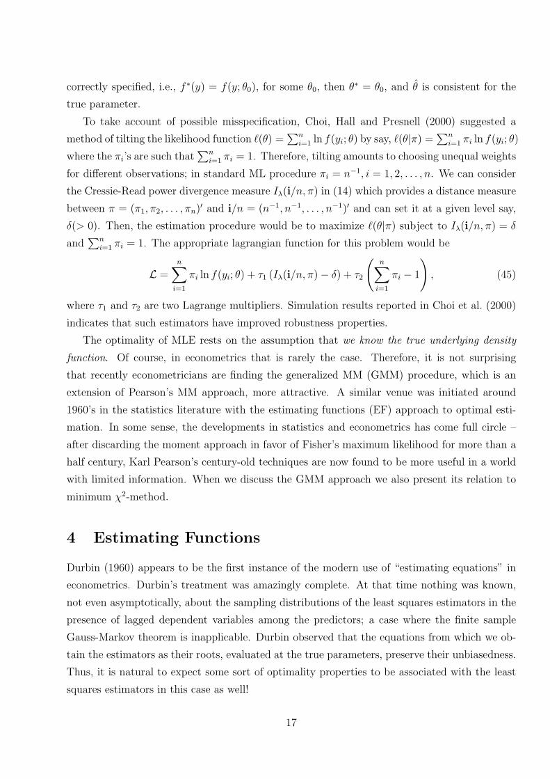
To take account of possible misspecification, Choi, Hall and Presnell (2000) suggested a

method of tilting the likelihood function `(θ) =∑n

i=1 ln f(yi; θ) by say, `(θ|π) =∑n

i=1 πi ln f(yi; θ)

where the πi’s are such that∑n

i=1 πi = 1. Therefore, tilting amounts to choosing unequal weights

for different observations; in standard ML procedure πi = n−1, i = 1, 2, . . . , n. We can consider

the Cressie-Read power divergence measure Iλ(i/n, π) in (14) which provides a distance measure

between π = (π1, π2, . . . , πn)′ and i/n = (n−1, n−1, . . . , n−1)′ and can set it at a given level say,

δ(> 0). Then, the estimation procedure would be to maximize `(θ|π) subject to Iλ(i/n, π) = δ

and∑n

i=1 πi = 1. The appropriate lagrangian function for this problem would be

L =n∑i=1

πi ln f(yi; θ) + τ1 (Iλ(i/n, π)− δ) + τ2

(n∑i=1

πi − 1

), (45)

where τ1 and τ2 are two Lagrange multipliers. Simulation results reported in Choi et al. (2000)

indicates that such estimators have improved robustness properties.

The optimality of MLE rests on the assumption that we know the true underlying density

function. Of course, in econometrics that is rarely the case. Therefore, it is not surprising

that recently econometricians are finding the generalized MM (GMM) procedure, which is an

extension of Pearson’s MM approach, more attractive. A similar venue was initiated around

1960’s in the statistics literature with the estimating functions (EF) approach to optimal esti-

mation. In some sense, the developments in statistics and econometrics has come full circle –

after discarding the moment approach in favor of Fisher’s maximum likelihood for more than a

half century, Karl Pearson’s century-old techniques are now found to be more useful in a world

with limited information. When we discuss the GMM approach we also present its relation to

minimum χ2-method.

4 Estimating Functions

Durbin (1960) appears to be the first instance of the modern use of “estimating equations” in

econometrics. Durbin’s treatment was amazingly complete. At that time nothing was known,

not even asymptotically, about the sampling distributions of the least squares estimators in the

presence of lagged dependent variables among the predictors; a case where the finite sample

Gauss-Markov theorem is inapplicable. Durbin observed that the equations from which we ob-

tain the estimators as their roots, evaluated at the true parameters, preserve their unbiasedness.

Thus, it is natural to expect some sort of optimality properties to be associated with the least

squares estimators in this case as well!

17

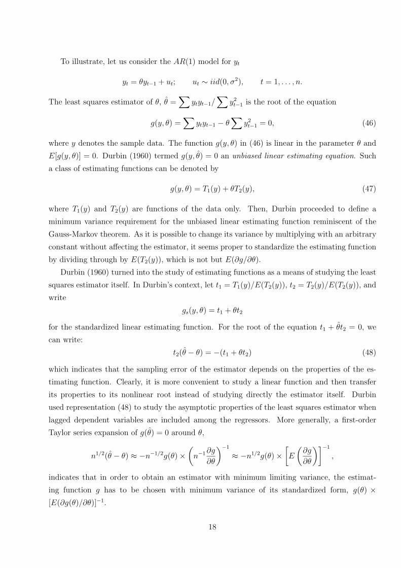
To illustrate, let us consider the AR(1) model for yt

yt = θyt−1 + ut; ut ∼ iid(0, σ2), t = 1, . . . , n.

The least squares estimator of θ, θ =∑

ytyt−1/∑

y2t−1 is the root of the equation

g(y, θ) =∑

ytyt−1 − θ∑

y2t−1 = 0, (46)

where y denotes the sample data. The function g(y, θ) in (46) is linear in the parameter θ and

E[g(y, θ)] = 0. Durbin (1960) termed g(y, θ) = 0 an unbiased linear estimating equation. Such

a class of estimating functions can be denoted by

g(y, θ) = T1(y) + θT2(y), (47)

where T1(y) and T2(y) are functions of the data only. Then, Durbin proceeded to define a

minimum variance requirement for the unbiased linear estimating function reminiscent of the

Gauss-Markov theorem. As it is possible to change its variance by multiplying with an arbitrary

constant without affecting the estimator, it seems proper to standardize the estimating function

by dividing through by E(T2(y)), which is not but E(∂g/∂θ).

Durbin (1960) turned into the study of estimating functions as a means of studying the least

squares estimator itself. In Durbin’s context, let t1 = T1(y)/E(T2(y)), t2 = T2(y)/E(T2(y)), and

write

gs(y, θ) = t1 + θt2

for the standardized linear estimating function. For the root of the equation t1 + θt2 = 0, we

can write:

t2(θ − θ) = −(t1 + θt2) (48)

which indicates that the sampling error of the estimator depends on the properties of the es-

timating function. Clearly, it is more convenient to study a linear function and then transfer

its properties to its nonlinear root instead of studying directly the estimator itself. Durbin

used representation (48) to study the asymptotic properties of the least squares estimator when

lagged dependent variables are included among the regressors. More generally, a first-order

Taylor series expansion of g(θ) = 0 around θ,

n1/2(θ − θ) ≈ −n−1/2g(θ)×(n−1∂g

∂θ

)−1

≈ −n1/2g(θ)×[E

(∂g

∂θ

)]−1

,

indicates that in order to obtain an estimator with minimum limiting variance, the estimat-

ing function g has to be chosen with minimum variance of its standardized form, g(θ) ×[E(∂g(θ)/∂θ)]−1.

18

Let G denote a class of unbiased estimating functions. Let

gs =g

E[∂g/∂θ](49)

be the standardized version of the estimating function g ∈ G. We will say that g∗ is the best

unbiased estimating function in the class G, if and only if, its standardized version has minimum

variance V ar(g∗s) in the class; that is

V ar(g∗s) ≤ V ar(gs) for all other g ∈ G. (50)

This optimality criterion was suggested by Godambe (1960) for general classes of estimating

functions and, independently, by Durbin (1960) for linear classes of estimating functions defined

in (47). The motivation behind the Godambe-Durbin criterion (50) as a way of choosing from

a class of unbiased estimating functions is intuitively sound: it is desirable that g is as close as

possible to zero when it is evaluated at the true value θ which suggests that we want V ar(g) to

be as small as possible. At the same time we want any deviation from the true parameter to

lead g as far away from zero as possible, which suggests that [E(∂g/∂θ)]2 be large. These two

goals can be accomplished simultaneously with the Godambe-Durbin optimality criterion that

minimizes the variance of gs in (49).

These developments can be seen as an analog of the Gauss-Markov theory for estimating

equations. Moreover, let `(θ) denote the loglikelihood function and differentiate E[g(y, θ)] = 0

to obtain E[∂g/∂θ] = −Cov[g, ∂`(θ)/∂θ]. Squaring both sides of this equality and applying the

Cauchy-Schwarz inequality yields the Cramer-Rao type inequality

E(g2)

[E (∂g/∂θ)]2≥ 1

E[(∂`(θ)/∂θ)2] , (51)

for estimating functions. Thus, a lower bound, given by the inverse of the information ma-

trix of the true density f(y; θ), can be obtained for V ar(g). Based on (51), Godambe (1960)

concluded that for every sample size, the score ∂`(θ)/∂θ is the optimum estimating function.

Concurrently, Durbin (1960) derived this result for the class of linear estimating equations. It

is worth stressing that it provides an exact or finite sample justification for the use of maximum

likelihood estimation. Recall that the usual justification of the likelihood-based methods, when

the starting point is the properties of the estimators, is asymptotic, as discussed in Section 3. A

related result is that the optimal estimating function within a class G has maximum correlation

with the true score function; cf. Heyde (1997). Since the true loglikelihood is rarely known, this

result is more useful from practical point of view.

Many other practical benefits can be achieved when working with the estimating functions

instead of the estimators. Estimating functions are much easier to combine and they are invariant

19

under one-to-one transformations of the parameters. Finally, the approach preserves the spirit of

the method of moments estimation and it is well suited for semiparametric models by requiring

only assumptions on a few moments.

Example 1: The estimating function (46) in the AR(1) model can be obtained in an al-

ternative way that sheds light to the distinctive nature of the theory of estimating functions.

Since E(ut) = 0, ut = yt − θyt−1, t = 1, 2, . . . , n are n elementary estimating functions. The

issue is how we should combine the n available functions to solve for the scalar parameter θ.

To be more specific, let ht be an elementary estimating function of y1, y2, . . . , yt and θ, with

Et−1(ht) ≡ E(ht|y1, . . . , yt−1) = 0. Then, by the law of iterated expectations E(hsht) = 0 for

s 6= t. Consider the class of estimating functions g

g =n∑t=1

at−1ht

created by using different weights at−1, which are dependent only on the conditioning event

(here, y1, . . . , yt−1). It is clear that, due to the law of iterated expectations, E(g) = 0. In this

class, Godambe (1985) showed that the quest for minimum variance of the standardized version

of g yields the formula for the optimal weights as

a∗t−1 =Et−1 (∂ht/∂θ)

Et−1(h2t )

. (52)

Application of (52) in the AR(1) model gives a∗t−1 = −yt−1/σ2, and so the optimal estimating

equation for θ is

g∗ =n∑t=1

yt−1(yt − θyt−1) = 0.

In summary, even if the errors are not normally distributed, the least squares estimating function

has some optimum qualifications once we restrict our attention to a particular class of estimating

functions.

Example 1 can be generalized further. Consider the scalar dependent variable yi with ex-

pectation E(yi) = µi(θ) modeled as a function of a p × 1 parameter vector θ; the vector of

explanatory variables xi, i = 1, . . . , n is omitted for convenience. Assume that the yi’s are inde-

pendent with variances V ar(yi) possibly dependent on θ. Then, the optimal choice within the

class of p× 1 unbiased estimating functions∑

i ai(θ)[yi − µi(θ)] is given by

g∗(θ) =n∑i=1

∂µi(θ)

∂θ

1

V ar(yi)[yi − µi(θ)], (53)

which involves only assumptions on the specification of the mean and variance (as it is the case

with the Gauss-Markov theorem). Wedderburn (1974) noticed that (53) is very close to the

20

true score of all the distributions that belong to the exponential family. In addition, g∗(θ) has

properties similar to those of a score function in the sense that,

1. E[g∗(θ)] = 0 and,

2. E[g∗(θ)g∗(θ)′] = −E[∂g∗(θ)/∂θ

′].

Wedderburn called the integral of g∗ in (53) “quasi-likelihood,” the equation g∗(θ) = 0 “quasi-

likelihood equation” and the root θ “maximum quasi-likelihood estimator.” Godambe and Heyde

(1987) obtained (53) as an optimal estimating function and assigned the name “quasi-score.”

This is a more general result in the sense that for its validity we do not need to assume that the

true underlying distribution belongs to the exponential family of distributions. The maximum

correlation between the optimal estimating function and the true unknown score justifies their

terminology for g∗(θ) as a “quasi-score.”

Example 2: Let yi, i = 1, . . . , n be independent random variables with E(yi) = µi(θ) and

V ar(yi) = σ2i (θ), where θ is a scalar parameter. The quasi-score approach suggests that in the

class of linear estimating functions we should solve

g∗(θ) =n∑i=1

[yi − µi(θ)]σ2i (θ)

∂µi(θ)

∂θ= 0. (54)

Under the assumption of normality of yi the maximum likelihood equation

∂`(θ)

∂θ= g∗(θ) +

1

2

n∑i=1

[yi − µi(θ)]2

σ4i (θ)

∂σ2i (θ)

∂θ− 1

2

n∑i=1

1

σ2i (θ)

∂σ2i (θ)

∂θ= 0, (55)

is globally optimal and the estimation based on the quasi-score (54) is inferior. If one were

unwilling to assume normality, one could claim that the weighted least squares approach that

minimizes∑

i[yi − µi(θ)]2/σ2i (θ) and yields the estimating equation

w(θ) = g∗(θ) +1

2

n∑i=1

[yi − µi(θ)]2

σ4i (θ)

∂σ2i (θ)

∂θ= 0 (56)

is preferable. However, because of the dependence of the variance on θ, (56) delivers an incon-

sistent root, in general; see Crowder (1986) and McLeish (1984). The application of a law of

large numbers shows that g∗(θ) is stochastically closer to the score (55) than is w(θ). In a way,

the second term in (56) creates a bias in w(θ), and the third term in (55) “corrects” for this bias

in the score equation. Here, we have a case in which the extremum estimator (weighted least

squares) is inconsistent, while the root of the quasi-score estimating function is consistent and

optimal within a certain class of estimating functions.

21

The theory of estimating functions has been extended to numerous other directions. For

extensions to dependent responses and optimal combination of higher-order moments, see Heyde

(1997) and the citations therein. For various applications see the volume edited by Godambe

(1991) and Vinod (1998). Li and Turtle (2000) offered an application of the EF approach in the

ARCH models.

5 Modern Approaches to Estimation in Econometrics

Pressured by the complicity of econometric models, econometricians looked for methods of

estimation that bypass the use of likelihood. This trend was also supported by the nature

of economic theories that do provide characterization of the stochastic laws only in terms of

moment restrictions; see Hall (2001) for specific examples. In the following we describe the

instrumental variables (IV) estimator, the generalized method of moments (GMM) estimator

and some recent extensions of GMM based on empirical likelihood. Often, the first instances

of these methods appear in the statistical literature. However, econometricians, faced with the

challenging task of estimating economic models, also offered new and interesting twists. We

start with Sargan’s (1958) IV estimation.

The use of IV was first proposed by Reiersøl (1941, 1945) as a method of consistent esti-

mation of linear relationships between variables that are characterized by measurement error.19

Subsequent developments were made by Geary (1948, 1949) and Durbin (1954). A definite

treatment of the estimation of linear economic relationships using instrumental variables was

presented by Sargan (1958, 1959).

In his seminal work, Sargan (1958) described the IV method as it is used currently in econo-

metrics, derived the asymptotic distribution of the estimator, solved the problem of utilizing

more instrumental variables than the regressors to be instrumented and discussed the similar-

ities of the method with other estimation methods available in the statistical literature. This

general theory was applied to time series data with autocorrelated residuals in Sargan (1959).

In the following we will use x to denote a regressor that is possibly subjected to measurement

error and z to denote an instrumental variable. It is assumed that a linear relationship holds,

yi = β1x1i + . . .+ βpxpi + ui; i = 1, . . . , n, (57)

19The history of IV estimation goes further back. In a series of work Wright (1920, 1921, 1925, 1928) advocated

a graphical approach to estimate simultaneous equation systems what he referred to as “path analysis.” In his

1971 Schultz Lecture, Goldberger (1972, p.938) noted: “Wright drew up a flow chart, . . . and read off the chart

a set of equations in which zero covariances are exploited to express moments among observable variables in

terms of structural parameters. In effect, he read off what we might now call instrumental-variable estimating

equations.” For other related references see Manski (1988, p.xii)

22

where the residual u in (57) includes a linear combination of the measurement errors in x’s.

In this case, the method of least squares yields inconsistent estimates of the parameter vector.

Reiersøl’s (1941, 1945) method of obtaining consistent estimates is equivalent to positing a zero

sample covariance between the residual and each instrumental variable. Then, we obtain p equa-

tions,∑n

i=1 zkiui = 0, k = 1, . . . , p, on the p parameters; the number of available instrumental

variables is assumed to be equal to the number of regressors.

It is convenient to express Reiersøl’s methodology in matrix form. Let Z be a (n× q) matrix

of instrumental variables with kth column z′k = (zk1, zk2 . . . , zkn)′, and for the time being we

take q = p. Likewise X is the (n× p) matrix of regressors, u the n× 1 vector of residuals and y

the n× 1 vector of responses. Then, the p estimating equations can be written more compactly

as

Z ′u = 0 or Z ′(y −Xβ) = 0, (58)

from which the simple IV estimator, β = (Z ′X)−1Z ′y, follows. Under the assumptions that

(i) plim n−1Z ′Z = ΣZZ , (ii) plim n−1Z ′X = ΣZX , and (iii) n−1/2Z ′u tends in distribution to

a normal vector with mean zero and covariance matrix σ2ΣZZ , it can be concluded that the

simple IV estimator β has a normal limiting distribution with covariance matrix V ar(n1/2β) =

σ2Σ−1ZXΣZZΣ−1

XZ [see Hall (1993)].

Reiersøl’s method of obtaining consistent estimates can be classified as an application of

the Pearson’s MM procedure.20 Each instrumental variable z induces the moment restriction

E(zu) = 0. In Reiersøl’s work, which Sargan (1958) developed rigorously, the number of these

moment restrictions that the data satisfy are equal to the number of unknown parameters.

A major accomplishment of Sargan (1958) was the study of the case in which the number of

available instrumental variables is greater than the number of regressors to be instrumented.

20There is also a connection between the IV and the limited information maximum likelihood (LIML) proce-

dures which generally is not mentioned in the literature. Interviewed in 1985 for the first issue of the Econometric

Theory, Dennis Sargan recorded this connection as his original motivation. Around 1950s Sargan was trying to

put together a simple Klein-type model for the UK, and his attempt to estimate this macroeconomic model led

him to propose the IV method of estimation as he stated [see Phillips (1985, p.123)]: “At that stage I also became

interested in the elementary methods of estimation and stumbled upon the method of instrumental variables as a

general approach. I did not become aware of the Cowles Foundation results, particularly the results of Anderson

and Rubin on LIML estimation until their work was published in the late 1940s. I realized it was very close to

instrumental variable estimation. The article which started me up was the article by Geary which was in the

JRSS in 1948. That took me back to the earlier work by Reiersøl, and I pretty early realized that the Geary

method was very close to LIML except he was using arbitrary functions of time as the instrumental variables,

particularly polynomials in the time variable. One could easily generalize the idea to the case, for example, of

using lagged endogenous variables to generate the instrumental variables. That is really where my instrumental

variable estimation started from.”

23

Any subset of p instrumental variables can be used to to form p equations for the consistent

estimation of the p parameters. Sargan (1958, pp.398-399) proposed that, p linear combinations

of the instrumental variables are constructed with the weights chosen so as to minimize the

covariance matrix of asymptotic distribution. More generally, if the available number of moment

restrictions exceeds that of the unknown parameters, p (optimal) linear combinations of the

moments can be used for estimation. This idea pretty much paved the way for the more recent

advances of the GMM approach in the history of econometric estimation and the testing of

overidentifying restrictions. As we show earlier, the way that the EF approach to optimal

estimation proceeds is very similar.

Specifically, suppose that there are q(> p) instrumental variables from which we construct a

reduced set of p variables z∗ki,

z∗ki =

q∑j=1

αkjzji, i = 1, . . . , n, k = 1, . . . , p.

Let us, for ease of notation, illustrate the solution to this problem using matrices. For any (q×p)weighting matrix α = [αkj] with rank[α] = p, Z∗ = Zα produces a new set of p instrumental

variables. Using Z∗ in the formula of simple IV estimator we obtain an estimator of β with

asymptotic distribution

√n(β − β)

d−→ N(0, σ2(α′ΣZX)−1(α′ΣZZα)(ΣXZα)−1). (59)

The next question is, which matrix α yields the minimum asymptotic variance-covariance matrix.

It can be shown that the optimal linear combination of the q instrumental variables is the one

that maximizes the correlation of Z∗ with the regressors X. Since the method of least squares

maximizes the squared correlation between the dependent variable and its fitted value, the

optimal (q × p) matrix α = [αkj] is found to be α0 = Σ−1ZZΣZX , for which it is checked that

0 ≤ [α(ΣXZα)−1 − α0(ΣXZα0)−1]′ΣZZ [α(ΣXZα)−1 − α0(ΣXZα0)−1]

= (α′ΣZX)−1α′ΣZZα(ΣXZα)−1 − (α′0ΣZX)−1α′0ΣZZα0(ΣXZα0)−1. (60)

In practice, α0 is consistently estimated by α0 = (Z ′Z)−1Z ′X and the proposed optimal

instrumental matrix is consistently estimated by the fitted value from regressing X on Z,

Z∗0 = Zα0 = Z(Z ′Z)−1Z ′X ≡ X. (61)

Then, the instrumental variables estimation methodology applies as before with Z∗0 ≡ X as the

set of instrumental variables. The set of estimating equations (58) is replaced by X′u = 0 which

in turn yields

β = (X′X)−1X

′y (62)

24

with covariance matrix of the limiting distribution V ar(n1/2β) = σ2(ΣXZΣ−1ZZΣZX)−1. This

estimator is termed generalized IV estimator as it uses the q(> p) available moments E(zju) = 0

j = 1, 2, . . . , q for estimating the p-vector parameter β. While Sargan (1958) combined the q

instrumental variables to form a new composite instrumental variable, the same result can be

obtained using the sample analogs of q moments themselves. This brings us back to the minimum

χ2 and the GMM approaches to estimation.

The minimum χ2 method and different variants are reviewed in Ferguson (1958). His article

also includes a new method of generating best asymptotically normal (BAN) estimates. These

methods are extremely close to what is known today in econometrics as the GMM. A recent

account is provided by Ferguson (1996). To illustrate, let us start with a q-vector sample

statistics Tn which is asymptotically normally distributed with E(Tn) = P (θ) and covariance

matrix V . The minimization of the quadratic form

Qn(θ) = n[Tn − P (θ)]′M [Tn − P (θ)], (63)

with respect to θ, was termed as minimum chi-square (χ2) estimation. In (63), the q× q matrix

M has the features of a covariance matrix that may or may not depend on θ and it is not

necessarily equal to V −1.

Clearly, the asymptotic variance of the minimum χ2 estimates θ depends on the choice of

the weighting matrix M . Let P be the q × p matrix of first partial derivatives of P (θ), where

for convenience we have omitted the dependence on θ. It can be shown√n(θ − θ) d→ N(0,Σ),

where

Σ = [P ′MP ]−1P ′MVMP [P ′MP ]−1. (64)

Assuming that V is nonsingular, M = V −1 is the optimal choice and the resulting asymptotic

variance Σ = [P ′V −1P ]−1 is minimum.

To reduce the computational burden and add flexibility in the generation of estimates that

are BAN, Ferguson (1958) suggested getting the estimates as roots of linear forms in certain

variables. Assuming that M does not depend on θ, the first order conditions of the minimization

problem (63)

−nP ′M [Tn − P (θ)] = 0 (65)

are linear combinations of the statistic [Tn−P (θ)] with weights P ′M . Based on this observation,

Ferguson (1958) considered equations using weights of general form. He went on to study the

weights that produce BAN estimates. This is reminiscent of the earlier EF approach but also

of the GMM approach that follows.

Example: (Optimality of the Pearson χ2 statistic in estimation) Consider the multinomial

probabilistic experiment with k classes and with probability of j-th class being qj(θ), j =

25

1, . . . , k; the dependence of each class probability on the unknown p-vector parameter θ is made

explicit. In this case the matrix V is given by

V = D0 −QQ′, (66)

where D0 = diag{q1(θ), q2(θ), . . . , qk(θ)} and Q′ = (q1(θ), q2(θ), . . . , qk(θ)). Ferguson (1958)

shows that if there is a nonsingular matrix V0 such that

V V0P = P , (67)

then the asymptotic variance of θ takes its minimum when the weights are given by the matrix

P ′V0 and the minimum value is Σ = [P ′V0P ]−1.

In this case, V in (66) is singular, but D−10 = diag{1/q1(θ), 1/q2(θ), . . . , 1/qk(θ)} satisfies

condition (67). Indeed, setting V0 = D−10 we get

V D−10 Q = Q, (68)

where Q is a k×p matrix of derivatives of Q with respect to θ. To see why the last equality holds

true, note that the 1× p vector Q′D−10 Q has typical element

∑kj=1 ∂qj(θ)/∂θi, which should be

zero by the fact that∑

j qj(θ) = 1. Pearson χ2 statistic uses precisely V0 = D−10 and therefore

the resulting estimators are efficient [see equation (11)]. Pearson χ2 statistic is an early example

of the optimal GMM approach to estimation.

Ferguson (1958) reformulated the minimum χ2 estimation problem in terms of estimating

equations. By interpreting the first order conditions of the problem as a linear combination

of elementary estimating functions, he realized that the scope of consistent estimation can be

greatly enhanced. In econometrics, Goldberger (1968, p.4) suggested the use of “analogy princi-

ple of estimation” as a way of forming the normal equations in the regression problem. However,

the use of this principle (or MM) instead of the least squares was not greatly appreciated at that

time.21 It was only with GMM that econometricians gave new force to the message delivered

by Ferguson (1958) and realized that IV estimation can be considered as a special case of a

more general approach. Hansen (1982) looked on the problem of consistent estimation from the

21In reviewing Goldberger (1968), Katti (1970) commented on the analogy principle as: “This is cute and will

help one remember the normal equations a little better. There is no hint in the chapter–and I believe no hints

exist–which would help locate such criteria in other situations, for example, in the problem of estimating the

parameters in the gamma distribution. Thus, this general looking method has not been shown to be capable

of doing anything that is not already known. Ad hoc as this method is, it is of course difficult to prove that

the criteria so obtained are unique or optimal.” Manski (1988, p.ix) acknowledged that he became aware of

Goldberger’s analogy principle only in 1984 when he started writing his book.

26

MM point of view.22 For instance, assuming that the covariance of each instrumental variable

with the residual is zero provided that the parameter is at its true value, the sample analog of

the covariance will be a consistent estimator of zero. Therefore, the root of the equation that

equates sample covariance to zero should be close to the true parameter. On the contrary, in

the case of regressors subjected to measurement errors, the normal equations X ′u = 0 will fail

to produce consistent estimates because the corresponding population moment condition is not

zero.

Let h(y; θ) be a general (q×1) function of data y and p-vector parameter θ, with the property

that for θ = θ0

E[h(y; θ0)] = 0. (69)

We say that the function h(y; θ) satisfies a moment or an orthogonality condition that holds true

only when θ is at its true value θ0. Alternatively, there are q moment conditions that can be

used to determine an estimate of the p-vector θ0. If q = p then

g(θ) ≡ 1

n

n∑i=1

h(yi; θ) = 0

will yield roots θ that are unique parameter estimates.

In the general case, in which q ≥ p, one can utilize Sargan’s idea and construct p “composite”

moment conditions by creating p linear combinations of those initial ones. More specifically,

Hansen proposed as GMM class of estimators the minimizers of the quadratic form

g(θ)′Ag(θ), (70)

where A is a (q × q) positive definite weighting matrix. The minimizer of (70) satisfies the p

equations of the first order conditions:[∂g(θ)

∂θ′

]′Ag(θ) = 0. (71)

That is, by applying GMM the estimation is based on p linear combinations of the moment

conditions with weights given by the p × q matrix [∂g(θ)/∂θ′]′A. The matrix A can be chosen

from an efficiency standpoint of view. Here, Hansen (1982) followed Sargan’s way of choosing

22From our conversation with Lars Hansen and Christopher Sims, we learned that a rudimentary form of GMM

estimator existed in Sims’ lecture notes. Hansen attended Sims’ lectures as a graduate student at the University

of Minnesota. Hansen formally wrote up the theories of GMM estimator and found its close connection to

Sargan’s (1958) IV estimator. To differentiate his paper, Hansen used a very general framework and established

the properties of the estimator under mild assumptions. In the econometrics literature, Hansen (1982) has been

the most influential paper to popularize the moment type and minimum χ2 estimation techniques.

27

linear combinations that minimize the covariance matrix of asymptotic distribution of the GMM

estimators. The result for the optimal A is known by now from Ferguson (1958) and the EF

approach discussed earlier: within the GMM class of estimators, we obtain the efficient one for

A = S−1, the inverse of the covariance matrix of the moment conditions. Likewise, the efficient

GMM estimator has covariance matrix equal to [g′0S−1g0]−1, where g0 = E[∂h(y; θ0)/∂θ]. In

practice, S is unknown and the GMM estimator needs a first step for the calculation of a

consistent estimate of S. Of course, the finite sample properties of the GMM estimator depend

on the estimate of S.

Hansen’s GMM has particular appeal to the economists who deal with a variety of moment

or orthogonality conditions derived from the theoretical properties of their postulated economic

models. Highly complex economic models make it difficult to write down a tractable likelihood

function. Then, the GMM approach provides a way to estimate model parameters consistently.

The methodology is very similar to the EF approach developed in the statistical literature.

However, the initial development of EF approach concerned with the optimal estimation. In

general, the use of optimal weighting matrices is impossible due to the presence of unknown

parameters; Newey (1993) has discussion on the feasible approaches to the efficient estimation.

Hansen’s GMM allows any weighting matrix [∂g(θ)/∂θ′]′A, thereby offering more flexibility in

practice. Moreover, the use of the objective function (70) offers a selection criterion among

multiple roots, a practical problem that is associated with the EF approach.

To see the connection of Hansen’s (1982) GMM estimation and Sargan’s (1958) IV estimation

[see also Hall (1993)], in the context of the classical linear regression model, with notation similar

to that utilized in the description of IV estimation, consider the q orthogonality (moment)

conditions

E(zku) = 0 k = 1, 2, . . . , q.

Using the GMM methodology, minimization of(Z ′u

n

)′A

(Z ′u

n

)with respect to β, in view of u = y −Xβ, yields first order conditions

−2X ′ZAZ ′(y −Xβ) = 0. (72)

If q = p, then (72) reduces to (58) which yields the simple IV estimator. Clearly, in case the

orthogonality conditions are equal to the number of unknown parameters, the β is just identified

and the choice of the weighting matrix A is inconsequential.

If q > p, the p × q matrix X ′ZA in (72) transforms the q (sample) moments Z ′(y − Xβ)

into p linear combinations that can be used to produce a unique solution for β. Now, different

28

choices of A will yield consistent estimates with different asymptotic variances. The discussion

earlier suggests that, in order to attain efficiency with the given set of q orthogonality conditions,

beyond a constant of proportionality, we should pickA = Σ−1ZZ ; in practice the consistent estimate

(n−1Z ′Z)−1 will be utilized. With that choice for A, the GMM estimator is identical to Sargan’s

generalized IV estimator (62). Now we turn our discussion to empirical likelihood (EL)-based

estimation that has recently become popular in econometrics.

In practice, inference based on the GMM as suggested by Hansen (1982) and its asymp-

totically equivalent forms suffers from poor finite sample properties; see for instance, Hansen,

Heaton and Yaron (1996) and, Pagan and Robertson (1997). The EL method proposed by Owen

(1988) has been fruitfully adapted to offer an alternative approach to inference in econometric

models: the empirical likelihood is maximized subject to the moment restrictions that data

satisfy in the population. Effectively, these methods impose the moment restrictions by appro-

priately reweighting the data. The resulting estimator of the unknown parameter is first-order

asymptotically equivalent to the efficient GMM estimator. Moreover, the sampling properties

of the estimators are similar to those supported by bootstrap, thus offering an increased chance

of finite-sample properties that are in accordance with asymptotic theory.

Let θ be the unknown parameter of primary interest. The moment condition E[h(y; θ)] = 0

holds at θ0, the true value of the parameter. Qin and Lawless (1994) proposed estimating the

parameter θ by solving the problem:

maxπi,θ

n∑i=1

lnπi s.t.n∑i=1

πi = 1,n∑i=1

πih(yi; θ) = 0, (73)

where each πi is restricted to be non-negative. This is equivalent to minimizing the entropy

measure (18) satisfying given moment conditions. The restriction∑

i πih(yi; θ) = 0 can be

interpreted as the empirical analog of the moment condition with πi being the probability of

the random variable y to take the value yi. This empirical analog differs from the one that is

used in the classical MM (or Hansen’s GMM) in that in the latter we assume πi = n−1 for every

observation yi. In the absence of the moment restriction∑

i πih(yi; θ) = 0 the above optimization

program is the non-parametric maximum log-likelihood that has the solution πi = n−1; each

sample observation is equally weighted. In the presence of the constraint the differentiation of

the lagrangian function

L =n∑i=1

lnπi + µ

(1−

n∑i=1

πi

)− nτ ′

n∑i=1

πih(yi; θ) (74)

yields estimated probabilities

πel,i =1

n[1 + τ ′elh(yi; θel)]. (75)

29

The estimated probabilities (75) differ from the uniform distribution, which assigns to each ob-

servation equal weight n−1, to the degree that the Lagrange multiplier vector of the moment

restriction τel, or tilting parameter, is away from zero or to the degree that the moment restric-

tion hold true. The EL approach for parameter estimation works by finding the multinomial

distribution (or, alternatively, the empirical probability distribution) π = (π1, π2, . . . , πn) that

accommodates the moment conditions. Now, the estimated probabilities are functions of θ.

Manipulation of the first-order conditions from the lagrangian (74) gives an alternative char-

acterization of the solution (θel, τel) that connects with the estimating function approach. The

estimators satisfy the equations∑n

i=1 ρel(yi; θel, τel) = 0, where

ρel(y; θ, τ) =

τ ′∂h(y; θ)

∂θ′[1 + τ ′h(y; θ)]−1

h(y; θ)[1 + τ ′h(y; θ)]−1

. (76)

The dimension of the multiplier τ is equal to the number of moment conditions given by the

dimension of the function h(y; θ). It can be shown that, under regularity conditions and for

the given set of moment conditions, θel is asymptotically equivalent to the efficient estimator

within the class of the GMM estimators. The efficient GMM estimator usually necessitates a

two-step procedure for the estimation of the best weighting matrix. In contrast, the empirical

likelihood approach requires only one-step, and this is expected to result in improved finite-

sample properties of estimators [see for example, Mittelhammer and Judge (2001)]. In other

words, as it is also emphasized in Mittelhammer et al. (2000, ch.12), the empirical likelihood

approach offers an operational way to optimally combine estimating equations.

Golan and Judge (1996), Imbens (1997), Imbens et al. (1998), and, Qin and Lawless (1994)

proposed a different objective function motivated by entropy or the Kullback-Leibler information

criterion (KLIC). This suggestion leads to the so-called exponential tilting (ET) estimator θet

of θ, which is based on the optimization problem [see also equation (20) and the discussion that

follows]

minπi,θ

n∑i=1

πilnπi s.t.n∑i=1

πi = 1,n∑i=1

πih(yi; θ) = 0. (77)

We denote the estimated Lagrange multiplier for the moment restrictions by τet. Again, the

solution yields estimated probabilities that are different from n−1:

πet,i =exp{τ ′eth(yi; θet)}∑ni=1 exp{τ ′eth(yi; θet)}

. (78)

The estimators in this problem satisfy the estimating equations∑n

i=1 ρet(yi; θet, τet) = 0, where

ρet(y; θ, τ) =

τ ′∂h(y; θ)

∂θ′exp{τ ′h(yi; θ)}

h(y; θ) exp{τ ′h(yi; θ)}

. (79)

30

The ET estimator was also suggested by Kitamura and Stutzer (1997) who handle the important

case of weakly dependent data. Their proposal utilizes the framework of linear inverse problems

and that allows them to propose convenient computational procedures. They show that the ET

estimators for (θ, τ) can be characterized by the optimization program

(θet, τet) = arg maxθ

minτ

n∑i=1

exp{τ ′h(yi; θ)}. (80)

From (80), it is easy to obtain the estimating functions given by (79). Similar characterization

can be made for the EL problem thereby yielding the set of just identified equations (76).

In the case of serially correlated observations Kitamura and Stutzer (1997) propose to smooth

the observations before the optimization and, in particular, to replace h(yi; θ) in (80) by

hi(θ) =K∑

k=−K

1

2K + 1h(yi−k, θ),

where K2/n→ 0, and K →∞ as n→∞.

The limiting distributions of the EL estimator θel and the ET estimator θet are identical; see

Imbens et al. (1998). They are both√n−consistent and asymptotically normal N(0,Σ), where

Σ =

{E

(∂h(y; θ0)

∂θ

)[E(h(y; θ0)h(y; θ0)′)]

−1E

(∂h(y; θ0)

∂θ

)}−1

, (81)

where the expectations are evaluated at the true value of parameter θ0. A consistent estimate

of Σ can be constructed by using the empirical analogs of each expectation involved. Efficiency

dictates that each observation yi is weighted by the estimated probability πi. For instance,

when working with the exponential tilting estimator E(h(y; θ0)h(y; θ0)′) will be estimated by∑i πet,ih(yi; θet)h(yi; θet)

′. However, consistency is not lost by using the uniform weights n−1.

Imbens et al. (1998) also show that the two estimators can be nested in a class of estimators

that arise from the minimization of the Cressie-Read power-divergence criterion (14) [Cressie and

Read (1984), Read and Cressie (1988)]. Consider two discrete distributions with common sup-

port p = (p1, p2, . . . , pn) and q = (q1, q2, . . . , qn) and rewrite the Cressie-Read power-divergence

criterion as

Iλ(p, q) =1

λ(1 + λ)

n∑i=1

pi

[(piqi

)λ− 1

], (82)

where λ is a given constant, and therefore, we can talk about a class of divergence criteria.

For given λ, the estimators for θ are defined so that the distance of the estimated probabilities

πi from the empirical distribution n−1 is minimized subject to the moment restrictions. More

specifically, let pi = n−1 and qi = πi. For fixed constant λ, we consider the minimization program

minπi,θ

Iλ(i/n, π) s.t.n∑i=1

πi = 1,n∑i=1

πih(yi; θ) = 0. (83)

31

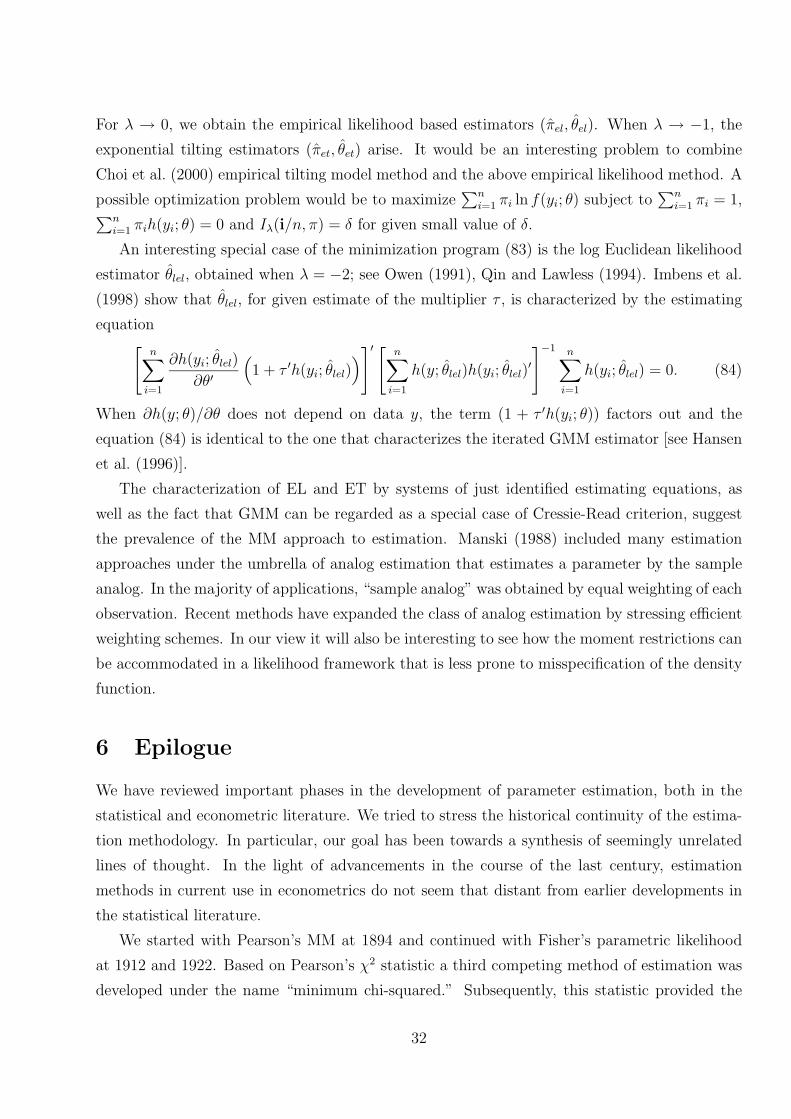
For λ → 0, we obtain the empirical likelihood based estimators (πel, θel). When λ → −1, the

exponential tilting estimators (πet, θet) arise. It would be an interesting problem to combine

Choi et al. (2000) empirical tilting model method and the above empirical likelihood method. A

possible optimization problem would be to maximize∑n

i=1 πi ln f(yi; θ) subject to∑n

i=1 πi = 1,∑ni=1 πih(yi; θ) = 0 and Iλ(i/n, π) = δ for given small value of δ.

An interesting special case of the minimization program (83) is the log Euclidean likelihood

estimator θlel, obtained when λ = −2; see Owen (1991), Qin and Lawless (1994). Imbens et al.

(1998) show that θlel, for given estimate of the multiplier τ , is characterized by the estimating

equation[n∑i=1

∂h(yi; θlel)

∂θ′

(1 + τ ′h(yi; θlel)

)]′ [ n∑i=1

h(y; θlel)h(yi; θlel)′

]−1 n∑i=1

h(yi; θlel) = 0. (84)

When ∂h(y; θ)/∂θ does not depend on data y, the term (1 + τ ′h(yi; θ)) factors out and the

equation (84) is identical to the one that characterizes the iterated GMM estimator [see Hansen

et al. (1996)].

The characterization of EL and ET by systems of just identified estimating equations, as

well as the fact that GMM can be regarded as a special case of Cressie-Read criterion, suggest

the prevalence of the MM approach to estimation. Manski (1988) included many estimation

approaches under the umbrella of analog estimation that estimates a parameter by the sample

analog. In the majority of applications, “sample analog” was obtained by equal weighting of each

observation. Recent methods have expanded the class of analog estimation by stressing efficient

weighting schemes. In our view it will also be interesting to see how the moment restrictions can

be accommodated in a likelihood framework that is less prone to misspecification of the density

function.

6 Epilogue

We have reviewed important phases in the development of parameter estimation, both in the

statistical and econometric literature. We tried to stress the historical continuity of the estima-

tion methodology. In particular, our goal has been towards a synthesis of seemingly unrelated

lines of thought. In the light of advancements in the course of the last century, estimation

methods in current use in econometrics do not seem that distant from earlier developments in

the statistical literature.

We started with Pearson’s MM at 1894 and continued with Fisher’s parametric likelihood

at 1912 and 1922. Based on Pearson’s χ2 statistic a third competing method of estimation was

developed under the name “minimum chi-squared.” Subsequently, this statistic provided the

32

basis for the development of a MM approach by Ferguson (1958), that was able to handle cases

where the number of available moments exceeds the number of unknown parameters. Parallel

lines of research were followed by Godambe (1960) and Durbin (1960) with the estimating func-

tion approach. More recently, in econometrics Hansen (1982) advocated the GMM procedure

that bears close resemblance to the last two approaches by Ferguson and Godambe-Durbin.

Nowadays, econometricians are moving away from the maximum likelihood estimation. The

nature of the conclusions derived from economic theorizing and the desire to avoid parametric

assumptions push the applied researcher to variants of the method of moments. At the onset of

the new century, after a long devotion to Fisher’s likelihood, the ideas of Pearson look more useful

than ever. It is our view that this interplay between Fisher’s concept of likelihood and Pearson’s

method of moments has resulted in an amazing synthesis that provides efficient estimation with

minimal model assumptions and very promising properties in finite samples.

These ideas have been blended fruitfully by the nonparametric method of empirical likeli-

hood. By using the Kullback-Leibler information criterion as a measure of the distance between

two distributions, we can also tie the method of moments to the concept of entropy. The current

state of affairs calls for more work on these estimation strategies. Maybe this task also calls for a

fresh reading of the old proposals; certainly, the close relationship between modern econometrics

with the ideas of Pearson and Fisher points to this direction.

In this review of the development of estimation, we have occasionally separated ourselves

from the riveting narrative and digressed to some side stories in statistics. In our view these

stories are important. Sometimes seemingly unambiguous description of different estimation

methodologies in econometrics textbooks brings temporary clarity to our confusions and helps

veil some of the parallel, and often-times much earlier, developments in the statistics literature.

It is worthwhile to record the initial motivation and historical progress in one place since the

original lines of development and philosophies become clouded by time. Although our overall aim

was too ambitious, this paper is essentially our first modest attempt, and some more research

along these lines would be profitable for students of econometrics.

Acknowledgements

We are grateful to Amos Golan and two anonymous referees for many helpful suggestions

that have considerably improved the paper. An earlier version of this paper under the title “A

Brief History of Estimation” was presented at a conference in honor of George Judge held at

the University of Illinois, May 1-2, 1999. We wish to acknowledge helpful comments from the

participants, in particular, from George Judge and Arnold Zellner. Kostas Fokianos, Alastair

Hall and Yuichi Kitamura kindly provided some extra references and/or detailed comments. We

33

would also like to thank Tatyana Dubovyk for providing very competent research assistance and

Naoko Miki for her help in preparing the manuscript. Special thanks are due to Amos Golan

without whose encouragement and kind prodding the paper would not have been completed.

However, we retain the responsibility for any remaining errors. Financial support from the

Office of Research, College of Commerce and Business Administration, University of Illinois

of Urbana-Champaign (for Anil Bera) and from University of Cyprus (for Yannis Bilias) is

gratefully acknowledged. This paper is dedicated to George Judge for his lifelong and continuing

contribution to econometrics.

References

Aldrich, J., 1997. R.A. Fisher and the making of maximum likelihood 1912-1922, Statistical

Science 12, 162-176.

Back, K., Brown, D. P., 1993. Implied probabilities in GMM estimators, Econometrica 61,

971-975.

Bennett, T. L., 1907-1908. Errors of observation, Technical Lecture, Number 4, Survey De-

partment, Ministry of Finance, National Printing Department, Cairo, Egypt.

Bera, A. K., 2000. Hypothesis testing in the 20th Century with a special reference to testing

with misspecified models, in: Rao, C. R., Szekely, G. J. eds., Statistics for the 21st Century

(Marcel Dekker, New York) 33-92.

Bera, A. K., Bilias, Y., 2000. The MM, ME, ML, EL, EF and GMM approaches to estimation:

A synthesis, Working Paper, Department of Economics, University of Illinois.

Bera, A. K., Bilias, Y., 2001. Rao’s score, Neyman’s C(α) and Silvey’s LM tests: An essay on

historical developments and some new results, Journal of Statistical Planning and Inference

97, forthcoming.

Bera, A. K., Ghosh, A., 2001. Neyman’s smooth test and its applications in econometrics,

in: Ullah, A., Wan, A., Chaturvedi, A. T. eds., Handbook of Applied Econometrics and

Statistical Inference (Marcel Dekker, New York), forthcoming.

Berger, J. O., 1985. Statistical Decision Theory and Bayesian Analysis (Springer-Verlag, New

York).

Berkson, J., 1980. Minimum chi-square, not maximum likelihood!, Annals of Statistics 8,

457-487.

Box, J. F., 1978. R. A. Fisher: The Life of a Scientist (John Wiley & Sons, New York).

Choi, E., Hall, P., Presnell, B., 2000. Rendering parametric procedures more robust by empir-

ically tilting the model, Biometrika 87, 453-465.

Cressie, N., Read, T. R. C., 1984. Multinomial goodness-of-fit tests, Journal of the Royal

Statistical Society 46, Series B, 440-464.

Cowell, F. A., 1980. On the structure of additive inequality measures, Review of Economic

Studies 47, 521-531.

34

Crowder, M., 1986. On consistency and inconsistency of estimating equations, Econometric

Theory 2, 305-330.

David, H. A., 1995. First (?) occurrence of common terms in mathematical statistics, American

Statistician 49, 121-133.

Durbin, J., 1954. Errors in variables, Review of Institute of International Statistics 22, 23-54.

Durbin, J., 1960. Estimation of parameters in time-series regression models, Journal of the

Royal Statistical Society 22, Series B, 139-153.

Edgeworth, F. Y., 1908. On the probable errors of frequency-constants, Journal of the Royal

Statistical Society 71, 381-397, 499-512, 651-678.

Edgeworth, F. Y., 1909. Addendum on “Probable errors of frequency-constants”, Journal of

the Royal Statistical Society 72, 81-90.

Edwards, A. W. F., 1997a. Three early papers on efficient parametric estimation, Statistical

Science 12, 35-47.

Edwards, A. W. F., 1997b. What did Fisher mean by ‘inverse probability’ in 1912-1922?,

Statistical Science 12, 177-184.

Engledow, F. L., Yule, G. U., 1914. The determination of the best value of the coupling-ratio

from a given set of data, Proceedings of the Cambridge Philosophical Society 17, 436-440.

Ferguson, T. S., 1958. A method of generating best asymptotically normal estimates with

application to estimation of bacterial densities. Annals of Mathematical Statistics 29,

1046-1062.

Ferguson, T. S., 1996. A Course in Large Sample Theory (Chapman & Hall, London).

Fisher, R. A., 1912. On an absolute criterion for fitting frequency curves, Messenger of Math-

ematics 41, 155-160.

Fisher, R. A., 1921. On the “probable error” of a coefficient of correlation deduced from a

small sample, Metron 1, 3-32.

Fisher, R. A., 1922. On the mathematical foundations of theoretical statistics, Philosophical

Transactions of the Royal Society of London 222, Series A, 309-368.

Fisher, R. A., 1924a. The conditions under which χ2 measures the discrepancy between obser-

vation and hypothesis, Journal of the Royal Statistical Society 87, 442-450.

Fisher, R. A., 1924b. On a distribution yielding the error functions of several well known

statistics, Proceedings of the International Congress of Mathematics (Toronto) 2, 805-813.

Fisher, R. A., 1928. Statistical Methods for Research Workers (Oliver and Boyd, Edinburgh).

Fisher, R. A., 1937. Professor Karl Pearson and the method of moments, Annals of Eugenics

7, 303-318.

Freeman, M. F., Tukey, J. W., 1950. Transformations related to the angular and the square

root, Annals of Mathematical Statistics 21, 607-611.

Galton, F., 1885. Regression towards mediocrity in hereditary stature, Journal of the Anthro-

pological Institute 15, 246-263.

Geary, R. C., 1948. Studies in the relations between economic time series, Journal of the Royal

Statistical Society 10, Series B, 140-158.

Geary, R. C., 1949. Determination of linear relations between systematic parts of variables

with errors of observation the variances of which are unknown, Econometrica 17, 30-58.

35

Geisser, S., 1980. Basic theory of the 1922 mathematical statistics paper, in: Fienberg, S. E.,

Hinkley, D. V. eds., R. A. Fisher: An Appreciation (Springer-Verlag, New York) 59-66.

Godambe, V. P., 1960. An optimum property of regular maximum likelihood estimation,

Annals of Mathematical Statistics 31, 1208-1212.

Godambe, V. P., 1985. The foundations of finite sample estimation in stochastic processes,

Biometrika 72, 419-428.

Godambe, V. P., ed., 1991. Estimating Functions (Oxford Science Publications, Oxford).

Godambe, V. P., Heyde, C. C., 1987. Quasi-likelihood and optimal estimation, International

Statistical Review 55, 231-244.

Gokhale, D. V., 1975. Maximum entropy characterizations of some distributions, in: Patil,

G. P., Kotz, S., Ord, J. K. eds., Statistical Distributions in Scientific Work, Volume 3 –

Characterizations and Applications (D. Reidel Publishing Company, Dordrecht) 299-304.

Golan, A., Judge, G., 1996. A maximum entropy approach to empirical likelihood estimation

and inference, University of California ARE Working Paper.

Golan, A., Judge, G., Miller, D., 1996. Maximum Entropy Econometrics: Robust Estimation

with Limited Data (John Wiley & Sons, New York).

Golan, A., Judge, G., Miller, D., 1997. The maximum entropy approach to estimation and

inference: An overview, in: Fomby, T.B., Hill, R. C. eds., Advances in Econometrics:

Applying Maximum Entropy to Econometric Problems (JAI Press, Greenwich) 3-24.

Golan, A., Judge, G., Miller, D., 1998. Information recovery in simultaneous-equations statis-

tical models, in: Ullah A., Giles, D. E. A. eds., Handbook of Applied Economic Statistics

(Marcel Dekker, New York) 365-381.

Goldberger, A. S., 1968. Topics in Regression Analysis (The Macmillan Company, New York).

Goldberger, A. S., 1972. Structural equation methods in the social sciences, Econometrica 40,

979-1001.

Grandy, W. T., Schick, L. H. eds., 1991. Maximum Entropy and Bayesian Methods (Kluwer

Academic Publishers, Dordrecht).

Haberman, S. J., 1984. Adjustment by minimum discriminant information, Annals of Statistics

12, 971-988.

Hacking, I., 1984. Trial by number, Science 84, 67-70.

Hald, A., 1998. A History of Mathematical Statistics form 1750 to 1930 (John Wiley & Sons,

New York).

Hald, A., 1999. On the history of maximum likelihood in relation to inverse probability and

least squares, Statistical Science 14, 214-222.

Haldane, J. B. S., 1919a. The probable errors of calculated linkage values, and the most

accurate methods of determining gametic from certain zygotic series, Journal of Genetics

8, 291-297.

Haldane, J. B. S., 1919b. The combination of linkage values, and the calculation of distances

between the loci of linked factors, Journal of Genetics 8, 299-309.

Hall, A., 1993. Some aspects of generalized method of moments estimation, in: Maddala, G.

S., Rao, C. R., Vinod, H. D. eds., Handbook of Statistics, Volume 11 (North Holland,

Amsterdam) 393-417.

36

Hall, A., 2001. Generalized method of moments, in: Baltagi, B., ed., A Companion to Theo-

retical Econometrics, (Blackwell Publishers, Oxford) 230-250.

Hansen, L., 1982. Large sample properties of generalized method of moments estimators,

Econometrica 50, 1029-1054.

Hansen, L., Heaton, J., Yaron, A., 1996. Finite sample properties of some alternative GMM

estimators, Journal of Business and Economic Statistics 14, 262-280.

Harris, J. A., 1912. A simple test of the goodness of fit of Mandelian ratios, American Naturalist

46, 741-745.

Heyde, C. C., 1997. Quasi-likelihood And Its Applications: A General Approach to Optimal

Parameter Estimation (Springer, New York).

Huber, P. J., 1967. The behavior of maximum likelihood estimates under nonstandard con-

ditions, in: Proceedings of Fifth Berkeley Symposium on Mathematical Statistics and

Probability (University of California Press, Berkeley), Volume 1, 221-233.

Imbens, G. W., 1997. One-step estimators for over-identified generalized method of moments

models, Review of Economic Studies 64, 359-383.

Imbens, G. W., Spady, R. H., Johnson, P., 1998. Information theoretic approaches to inference

in moment condition models, Econometrica 66, 333-357.

Jaynes, E. T., 1957. Information theory and statistical mechanics, Physical Review 106, 620-

630.

Kagan, A. M., Linnik, Y. V., Rao, C. R., 1973. Characterization Problems in: Mathematical

Statistics (John Wiley & Sons, New York).

Katti, S. K., 1970. Review of “Topics in Regression Analysis”, Econometrica 38, 945-946.

Kent, J. T., 1982. Robust properties of likelihood ratio tests, Biometrika 69, 19-27.

Kitamura, Y., Stutzer, M., 1997. An information theoretic alternate to generalized method of

moments estimation, Econometrica 65, 861-874.

Koenker, R., 2000. Galton, Edgeworth, Frisch, and prospect for quantile regression in econo-

metrics, Journal of Econometrics 95, 347-374.

Le Cam, L., 1990. Maximum likelihood: An introduction, International Statistical Review 58,

153-171.

Lehmann, E. L., 1999. “Student” and small-sample theory, Statistical Science 14, 418-426.

Li, D. X., Turtle, H. J., 2000. Semiparametric ARCH models: An estimating function approach.

Journal of Business and Economic Statistics , 175-186.

Lindsay, B. G., 1994. Efficiency versus robustness: The case for minimum Hellinger distance

and related methods, Annals of Statistics 22, 1081-1114.

Maasoumi, E., 1993. A compendium to information theory in economics and econometrics,

Econometric Reviews 12, 137-181.

Manski, C., 1988. Analog Estimation Methods in Econometrics (Chapman and Hall, London).

Mardia, K. V., 1975. Characterization of directional distributions, in: Patil, G. P., Kotz, S.,

Ord, J. K. eds., Statistical Distributions in Scientific Work, Volume 3 – Characterizations

and Applications (D. Reidel Publishing Company, Dordrecht) 365-385.

McLeish, D. L., 1984. Estimation for aggregate models: The aggregate Markov chain, Canadian

Journal of Statistics 12, 265-282.

37

Mensch, R., 1980. Fisher and the method of moments, in: Fienberg, S.E., Hinkley, D. V. eds.,

R. A. Fisher: An Appreciation (Springer-Verlag, New York) 67-74.

Mittelhammer, R. C., Judge, G. G., 2001. Finite sample performance of empirical likelihood

under endogeneity, Discussion Paper, University of California, Berkeley.

Mittelhammer, R. C., Judge, G. G., Miller, D. J., 2000. Econometric Foundations (Cambridge

University Press, Cambridge).

Newey, W. K., 1993. Efficient estimation of models with conditional moment restrictions, in:

Maddala, G. S., Rao, C. R., Vinod, H. D., eds., Handbook of Statistics, Volume 11 (North

Holland, Amsterdam) 419-454.

Neyman, J., 1937. “Smooth test” for goodness of fit, Skand. Akturarietidskr 20, 150-199.

Neyman, J., 1949. Contribution to the theory of the χ2 test, in: Proceedings of the Berkeley

Symposium on Mathematical Statistics and Probability (University of California Press,

Berkeley) 329-273.

Neyman, J., 1967. R.A. Fisher (1890-1962): An appreciation, Science 156, 1456-1460.

Neyman, J., Pearson, E. S., 1928. On the use and interpretation of certain test criteria for

purpose of statistical inference, Part II, Biometrika 20, 263-294.

Owen, A., 1988. Empirical likelihood ratio confidence intervals for a single functional, Biometrika

75, 237-249.

Owen, A., 1990. Empirical likelihood confidence regions, Annals of Statistics 18, 90-120.

Owen, A., 1991. Empirical likelihood for linear models, Annals of Statistics 19, 1725-1747.

Pagan, A. R., Robertson, J., 1997. GMM and its problems, manuscript, Australian National

University.

Pearson, E. S., 1936. Karl Pearson: An appreciation of some aspects of his life and work,

Biometrika 28, 193-257.

Pearson, K., 1894. Contribution to the mathematical theory of evolution, Philosophical Trans-

actions of the Royal Society of London 185, Series A, 71-110.

Pearson, K., 1895. Skew variation in homogeneous material, Philosophical Transactions of the

Royal Society of London 186, Series A, 343-414.

Pearson, K., 1900. On the criterion that a given system of deviations from the probable in the

case of a correlated system of variables is such that it can be reasonably supposed to have

arisen from random sampling, Philosophical Magazine Series 50, 157-175.

Pearson, K., 1902. On the systematic fitting of curves to observations and measurements, Parts

I and II, Biometrika 1, 265-303; 2, 1-23.

Pearson, K., 1936. Method of moments and method of maximum likelihood, Biometrika 28,

34-59.

Phillips, P. C. B., 1985. ET interviews: Professor J. D. Sargan, Econometric Theory 1, 119-

139.

Pompe, B., 1994. On some entropy methods in data analysis, Chaos, Solitons and Fractals 4,

83-96.

Qin, J., Lawless, J., 1994. Empirical likelihood and general estimating equations, Annals of

Statistics 22, 300-325.

38

Read, T. R. C., Cressie, N., 1988. Goodness-of-Fit Statistics for Discrete Multivariate Data

(Springer-Verlag, New York).

Renyi, A., 1961. On measures of entropy and information, Proceedings of the Fourth Berkeley

Symposium on Mathematics, Statistics, and Probability (University of California Press,

Berkeley) Volume 1, 547-561.

Reiersøl, O., 1941. Confluence analysis by means of lag moments and other methods of con-

fluence analysis, Econometrica 9, 1-23.

Reiersøl, O., 1945. Confluence Analysis by Means of Sets of Instrumental Variables (Almquist

& Wiksell, Uppsala).

Sargan, J. D., 1958. The estimation of economic relationships using instrumental variables,

Econometrica 26, 393-415.

Sargan, J. D., 1959. The estimation of relationships with auto-correlated residuals by the use

of instrumental variables, Journal of the Royal Statistical Society 21, Series B, 91-105.

Savage, L. J., 1976. On rereading R. A. Fisher, Annals of Statistics 4, 441-483.

Schutzenberger, M. P., (1954). Contribution aux applications statistiques de la theorie de l’

information, Publication of the Institute of Statistics, University of Paris.

Sen, A. K., 1975. On Economic Inequality (Claredon Press, Oxford).

Shannon, C. E., Weaver, W., 1949. The Mathematical Theory of Communication (University

of Illinois Press, Urbana).

Shenton, L. R., 1950. Maximum likelihood and the efficiency of the method of moments,

Biometrika 37, 111-116.

Shenton, L. R., 1958. Moment estimators and maximum likelihood, Biometrika 45, 411-420.

Shenton, L. R., 1959. The distribution of moment estimators, Biometrika 46, 296-305.

Shorrocks, A. F., 1980. The class of additively decomposable inequality measures, Economet-

rica 48, 613-625.

Smith, K., 1916. On the ‘best’ values of the constants in the frequency distributions, Biometrika

11, 262-276.

Steven, S. S., (1975). Psychophysics (John Wiley, New York).

Stigler, S. M., 1976. Comment on “On rereading R. A. Fisher”, Annals of Statistics 4, 498-500.

Student, 1908. The probable error of a mean, Biometrika 6, 1-25.

Ullah, A., 1996. Entropy, divergence and distance measures with econometric applications,

Journal of Statistical Planning and Inference 49, 137-162.

Urzua, C. M., 1988. A class of maximum-entropy multivariate distributions, Communications

in Statistics: Theory and Method 17, 4039-4057.

Urzua, C. M., 1997. Omnibus tests for multivariate normality based on a class of maximum

entropy distributions, in: Fomby, T. B., Hill, R. C. eds., Advances in Econometrics: Ap-

plying Maximum Entropy to Econometric Problems (JAI Press, Greenwich) 341-358.

Vinod, H. D., 1998. Foundations of statistical inference based on numerical roots of robust

pivot functions, Journal of Econometrics 86, 387-396.

Wedderburn, R. W. M., 1974. Quasi-likelihood functions, generalized linear models, and the

Gauss-Newton method, Biometrika 61, 439-447.

39

White, H., 1982. Maximum likelihood estimation of misspecified models, Econometrica 50,

1-26.

Wilks, S. S., 1943. Mathematical Statistics (Princeton University Press, Princeton)

Wright, S., 1920. The relative importance of heredity and environment in determining the

birth weight of guinea pigs, Proceedings of the National Academy of Sciences 6, 320-332.

Wright, S., 1921. Correlation and causation, Journal of Agricultural Research 20, 557-585.

Wright, S., 1925. Corn and hog correlations, U.S. Department of Agriculture Bulletin 1300,

Washington.

Wright, S., 1928. Appendix to Wright, P. The Traffic on Animal and Vegetable Oils (Macmillan,

New York).

Zellner, A., 1991. Bayesian methods and entropy in economics and econometrics, in: Grandy,

W. T., Schick, L. H. eds., Maximum Entropy and Bayesian Methods (Kluwer Academic

Publishers, Dordrecht) 17-31.

Zellner, A., 1997. Bayesian method of moments (BMOM): Theory and applications, in: Fomby,

T. B., Hill, R. C. eds., Advances in Econometrics: Applying Maximum Entropy to Econo-

metric Problems (JAI Press, Greenwich) 85-105.

Zellner, A., Highfield, R., 1988. Calculation of maximum entropy distributions and approxi-

mation of marginal posterior distributions, Journal of Econometrics 37, 195-209.

40

SELECTED RECENT PUBLICATIONS

Bera A. K. and Yannis Bilias, Rao´s Score, Neyman´s C ($\alpha$) and Silvey´s LM Tests:An Essay on Historical Developments and Some New Results, Journal of StatisticalPlanning and Inference, forthcoming.

Bertaut C. and M. Haliassos, Precautionary Portfolio Behavior from a Life - CyclePerspective, Journal of Economic Dynamics and Control, 21, 1511-1542, 1997.

Bilias Y., Minggao Gu and Zhiliang Ying, Towards a General Asymptotic Theory for theCox model with Staggered Entry, The Annals of Statistics, 25, 662-682, 1997.

Blundell R., P. Pashardes and G. Weber, What Do We Learn About Consumer DemandPatterns From Micro-Data?, American Economic Review, 83, 570-597, 1993.

Bougheas S., P. Demetriades and T. P. Mamouneas, Infrastructure, Specialization andEconomic Growth, Canadian Journal of Economics, forthcoming.

Caporale W., C. Hassapis and N. Pittis, Unit Roots and Long Run Causality: Investigating theRelationship between Output, Money and Interest Rates, Economic Modeling, 15(1), 91-112,January 1998.

Caporale G. and N. Pittis, Efficient estimation of cointegrated vectors and testing forcausality in vector autoregressions: A survey of the theoretical literature, Journal ofEconomic Surveys, forthcoming.

Caporale G. and N. Pittis, Unit root testing using covariates: Some theory and evidence,Oxford Bulletin of Economics and Statistics, forthcoming.

Caporale G. and N. Pittis, Causality and Forecasting in Incomplete Systems, Journal ofForecasting, 16, 6, 425-437, 1997.

Clerides K. S., Lach S. and J.R. Tybout, Is Learning-by-Exporting Important? Micro-Dynamic Evidence from Colombia, Morocco, and Mexico, Quarterly Journal of Economics113(3), 903- 947, August 1998.

Cukierman A., P. Kalaitzidakis, L. Summers and S. Webb, Central Bank Independence,Growth, Investment, and Real Rates", Reprinted in Sylvester Eijffinger (ed), IndependentCentral Banks and Economic Performance, Edward Elgar, 416-461, 1997.

Dickens R., V. Fry and P. Pashardes, Non-Linearities and Equivalence Scales, The EconomicJournal, 103, 359-368, 1993.

Demetriades P. and T. P. Mamuneas, Intertemporal Output and Employment Effects ofPublic Infrastructure Capital: Evidence from 12 OECD Economies, Economic Journal, July2000.

Eicher Th. and P. Kalaitzidakis, The Human Capital Dimension to Foreign DirectInvestment: Training, Adverse Selection and Firm Location”. In Bjarne Jensen and Kar-yiu

Wong (eds), Dynamics,Economic Growth, and International Trade, The University ofMichigan Press, 337-364, 1997.

Fry V. and P. Pashardes, Abstention and Aggregation in Consumer Demand, OxfordEconomic Papers, 46, 502-518, 1994.

Gatsios K., P. Hatzipanayotou and M. S. Michael, International Migration, the Provision ofPublic Good and Welfare, Journal of Development Economics, 60/2, 561-577, 1999.

Haliassos M. and C. Hassapis, Non-expected Utility, saving, and Portfolios, The EconomicJournal, 110, 1-35, January 2001.

Haliassos M. and J. Tobin, The Macroeconomics of Government Finance, reprinted inJ.Tobin, Essays in Economics, vol. 4, Cambridge: MIT Press, 1996.

Haliassos M. and C. Bertaut, Why Do So Few Hold Stocks?, The Economic Journal, 105,1110- 1129, 1995.

Haliassos M., On Perfect Foresight Models of a Stochastic World, Economic Journal, 104,477-491, 1994.

Hassapis C., N. Pittis and K. Prodromidis, Unit Roots and Granger Causality in the EMSInterest Rates: The German Dominance Hypothesis Revisited, Journal of InternationalMoney and Finance, 18(1), 47-73, 1999.

Hassapis C., S. Kalyvitis and N. Pittis, Cointegration and Joint Efficiency of InternationalCommodity Markets”, The Quarterly Review of Economics and Finance, 39, 213-231, 1999.

Hassapis C., N. Pittis and K. Prodromides, EMS Interest Rates: The German DominanceHypothesis or Else?” in European Union at the Crossroads: A Critical Analysis of MonetaryUnion and Enlargement, Aldershot, UK., Chapter 3, 32-54, 1998. Edward Elgar PublishingLimited.

Hatzipanayotou P., and M. S. Michael, General Equilibrium Effects of Import ConstraintsUnder Variable Labor Supply, Public Goods and Income Taxes, Economica, 66, 389-401,1999.

Hatzipanayotou, P. and M.S. Michael, Public Good Production, Nontraded Goods and TradeRestriction, Southern Economic Journal, 63, 4, 1100-1107, 1997.

Hatzipanayotou, P. and M. S. Michael, Real Exchange Rate Effects of Fiscal ExpansionUnder Trade Restrictions, Canadian Journal of Economics, 30-1, 42-56, 1997.

Kalaitzidakis P., T. P. Mamuneas and Th. Stengos, A Nonlinear Sensitivity Analysis ofCross-Country Growth Regressions, Canadian Journal of Economics, forthcoming.

Kalaitzidakis P., T. P. Mamuneas and Th. Stengos, European Economics: An Analysis Basedon Publications in Core Journals, European Economic Review, 43, 1150-1168, 1999.

Kalaitzidakis P., On-the-job Training Under Firm-Specific Innovations and WorkerHeterogeneity, Industrial Relations, 36, 371-390, July 1997.

Ludvigson S. and A. Michaelides, Does Buffer Stock Saving Explain the Smoothness andExcess Sensitivity of Consumption?, American Economic Review, forthcoming

Lyssiotou Panayiota, Dynamic Analysis of British Demand for Tourism Abroad, EmpiricalEconomics, forthcoming, 2000.

Lyssiotou P., P. Pashardes and Th. Stengos, Testing the Rank of Engel Curves withEndogenous Expenditure, Economics Letters, 64, 61-65, 1999.

Lyssiotou P., P. Pashardes and Th. Stengos, Preference Heterogeneity and the Rank ofDemand Systems, Journal of Business and Economic Statistics, 17 (2), 248-252, April 1999.

Lyssiotou Panayiota, Comparison of Alternative Tax and Transfer Treatment of Childrenusing Adult Equivalence Scales, Review of Income and Wealth, 43 (1), 105-117, March 1997.

Mamuneas, Theofanis P., Spillovers from Publicly – Financed R&D Capital in High-TechIndustries, International Journal of Industrial Organization, 17(2), 215-239, 1999.

Mamuneas, T. P. and Nadiri M. I., R&D Tax Incentives and Manufacturing-Sector R&DExpenditures, in Borderline Case: International Tax Policy, Corporate Research andDevelopment, and Investment, James Poterba (ed.), National Academy Press, WashingtonD.C., 1997. Reprinted in Chemtech, 28(9), 1998.

Mamuneas, T. P. and Nadiri M. I., Public R&D Policies and Cost Behavior of the USManufacturing Industries, Journal of Public Economics, 63, 57-81, 1996.

Michaelides A. and Ng, S., Estimating the Rational Expectations Model of SpeculativeStorage: A Monte Carlo Comparison of three Simulation Estimators, Journal ofEconometrics, 96(2), 231-266, 2000.

Pashardes Panos, Equivalence Scales in a Rank-3 Demand System, Journal of PublicEconomics, 58, 143-158, 1995.

Pashardes Panos, Bias in Estimating Equivalence Scales from Grouped Data, Journal ofIncome Distribution, Special Issue: Symposium on Equivalence Scales, 4, 253-264,1995.

Pashardes Panos., Bias in Estimation of the Almost Ideal Demand System with the StoneIndex Approximation, Economic Journal, 103, 908-916, 1993.

Spanos Aris, Revisiting Date Mining: ´Hunting´ With or Without a License, Journal ofMethodology, July 2000.

Spanos Aris, On Normality and the Linear Regression Model, Econometric Reviews, 14,195-203, 1995.

Spanos Aris, On Theory Testing in Econometrics: Modeling with nonexperimental Data,Journal of Econometrics, 67, 189-226, 1995.

Spanos Aris, On Modeling Heteroscedasticity: The Student's t and Elliptical LinearRegression Models, Econometric Theory, 10, 286-315, 1994.