Force fields for coarse-grained molecular

simulations from a corresponding states correlation

Andrés Mejía a, Carmelo Herdes b, Erich A. Müller b *

a Departamento de Ingeniería Química, Universidad de Concepción, Chile.

b Department of Chemical Engineering, Imperial College London, U. K.

* corresponding author , E-mail: e.muller@imperial.ac.uk

ABSTRACT

We present a corresponding states correlation based on the description of fluid phase

properties by means of a Mie intermolecular potential applied to tangentially-bonded

spheres. The macroscopic properties of this model fluid are very accurately

represented by a recently proposed version of the statistical associating fluid theory

(the SAFT- version). The Mie potential can be expressed in a conformal manner in

terms of three parameters that relate to a length scale, , an energy scale, and the

range or functional form of the potential, , while the non-sphericity or elongation of

a molecule can be appropriately described by the chain length, m. For a given chain

length, correlations are given to scale the SAFT equation of state in terms of three

experimental parameters: the acentric factor, the critical temperature and the saturated

liquid density at a reduced temperature of 0.7. The molecular nature of the equation of

state is exploited to make a direct link between the macroscopic thermodynamic

1

parameters used to characterize the equation of state and the parameters of the

underlying Mie potential. This direct link between macroscopic properties and

molecular parameters is the basis to propose a top-down method to parametrize force

fields that can be used in the coarse grained molecular modelling (Monte Carlo or

molecular dynamics) of fluids. The resulting correlation is of quantitative accuracy

and examples of the prediction of simulations of vapour-liquid equilibria and

interfacial tensions are given. In essence, we present a recipe that allows one to obtain

intermolecular potentials for use in the molecular simulation of simple and chain

fluids from macroscopic experimentally determined constants, namely the acentric

factor, the critical temperature and a liquid density.

Keywords SAFT, intermolecular potentials, parameters, fluids, coarse graining,

multiscale modelling

1. Introduction

The corresponding states principle stems from the empirical observation that the

behaviour of most common fluids may be described in a generalized way if the

variables that describe their thermodynamic states are scaled accordingly. Much in the

same way as Leonardo da Vinci’s Vitruvian Man exemplified a canon of proportions

for the human body, the corresponding states principle was originally derived as a

heuristic relationship which allowed the mapping of volumetric properties of fluids

into unique generalized graphs and equations.

2

There is a myriad of empirical and semi-theoretical approaches that apply the

corresponding state principle1,2. In engineering, most are based on the use of the

critical properties of the vapor-liquid transition, e.g. the critical pressure, Pc, the

critical temperature, Tc, the critical density, c ; or some combination thereof, e.g. the

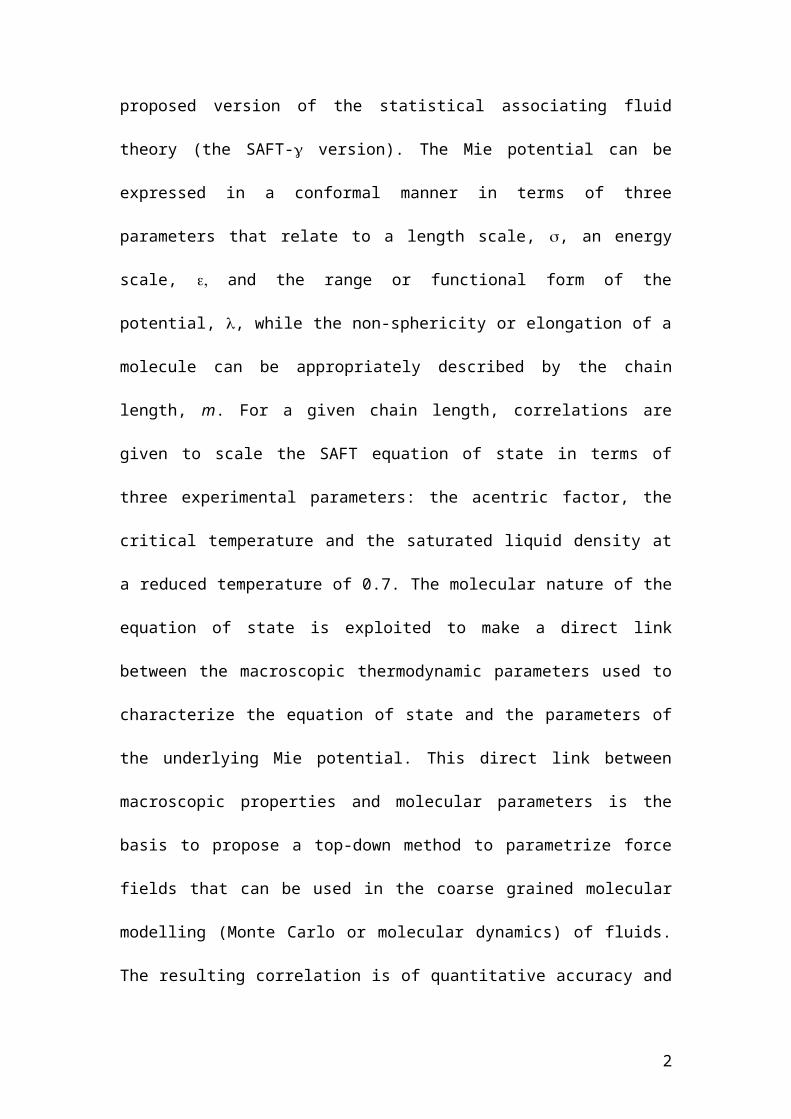
critical compressibility factor, Zc. A prototypical example championed originally by

van der Waals 3, is that based on his equation of state (EoS) 4

(1)

Where P is the pressure, T is the temperature, the density and R the ideal gas

constant. The two additional constants, the co-volume, b, and the cohesion factor, a,

may be determined by forcing the equation to pass through the critical point and the

critical isotherm to have an inflexion point at the critical point. By doing this both

constants become unique and defined in terms of the critical point itself,

(2)

One can see from that above, that the fluid phase behaviour is completely specified by

the fixing any pair of critical constants (although Tc and Pc are usually chosen). The

previous approach to the description of volumetric properties is frequently referred to

as a two-parameter corresponding states model in reference to the characteristic scales

employed to non-dimensionalize the relations.

3

Derivations of the van der Waals EoS based on statistical thermodynamics 5, 6

illustrate how one may establish a relation between the EoS and an underlying

Sutherland pair potential, where molecules are described as hard core spheres with a

central attractive potential which decays as –(/r)6 , r being the interparticle

distance, the minimum energy well depth and the hard sphere diameter. It can be

shown that the two constants in the van der Waals treatment may then alternatively

related to intermolecular potential parameters,

(3)

where Nav is Avogadro’s number. Comparing equations (2) and (3) one can

immediately establish a link between the macroscopic description of fluids through an

EoS and the molecular description, which relates these parameters to intermolecular

size and energy parameters. Unfortunately, in order to derive a closed-form analytical

expression for the macroscopic thermodynamic properties from the potential, some

approximations (e.g., additivity of excluded volumes, a mean-field treatment of the

attractive contribution) must be made, which decouple the correspondence between

the EoS to the precise form of the underlying microscopic model, i.e., the van der

Waals EoS would not be able to model accurately a fluid that behaves following the

Sutherland potential. Furthermore, neither the van der Waals equation nor the related

potential are accurate enough for our current requests for the fitting of experimental

data.

4

Figure 1 : Temperature, T – density, , phase diagram of an attractive

sphere (solid line) and the corresponding trimer (dashed-dotted) oligomer

formed by spheres of the same type.

A more complicated scenario arises if one is willing to recognize that the non-

sphericity, particularly in the context of elongated and chain-like fluids, has a

profound effect on the vapor-liquid equilibria. Figure 1 shows the corresponding

temperature-density plot of a fluid of spheres, as compared to a fluid composed of a

chain of three linear tangentially joined spheres (an oligomer of the latter). It is

apparent how elongation of a molecule increases the critical temperature, decreases

the number density and changes the slope of the vapor-pressure curve (not shown). It

is clear that these two fluids (the monomer and the chain) cannot be conformal, i.e. do

not obey a two-parameter corresponding principle in the terms stated above, i.e. they

cannot be described with the a unique intermolecular potential having only two scales,

(in this case and . This restriction on conformality was recognized decades ago;

5

the most salient example of this was the Soave7 modification of the van der Waals

model. Upon using a cubic EoS to attempt to fit the n-alkane series, Soave recognized

the above behaviour and included in his equation of state an additional parameter that

could, in principle, account for this. The third parameter (along with the previous

ones, Tc and Pc) was Pitzer’s acentric factor, , defined as 8

(4)

The acentric factor is an empirical constant, based on the observation that for the

heavier noble gases, the base 10 logarithm of the ratio of the saturation pressure to the

critical pressure at a given point of the vapour pressure curve (T/Tc = 0.7) is

numerically equal to (-1). The acentric factor of noble gases is by construction equal

to zero, and for most simple fluids is a small positive number that quantifies the

deviation of the slope of the vapor pressure curve from that of the “idealized”

spherical fluid. As a fortunate aside, it happens that other deviations from the simple

dispersion model found in a noble gas: polarity, polarizability, hydrogen bonding,

non-sphericity; all contribute to the change in slope of the vapor pressure curve in the

same fashion, hence a single parameter may be used to fit all the previously

mentioned non-conformalities.

6

Figure 2 Effect of intermolecular interactions on the slope of the vapor

pressure curve. The ordinate corresponds to the base 10 log of the ratio of

the vapor pressure to the critical point (corresponding to -1-. For the

noble gases this takes on the value of zero, and becomes larger as the

interaction deviates either because of non-sphericity (e.g. n-C10H22) and/or as

a consequence of deviations from simple dispersive interactions (e.g. CF4)

The three-parameter corresponding states (3PCS) correlation based on the inclusion of

the acentric factor, e.g. using variables such as Tc , Pc and for describing the

universality of fluid behaviour, has become a staple of chemical and process

engineering. Notwithstanding its success, the grouping of all deviations from simple

spherical molecules in a single parameter such as the acentric factor, fails to

distinguish between the effects mainly attributable to size asymmetry and those

related to the range of the intermolecular potential. Empirical attempts to separate

7

these effects lead to four-parameter corresponding states correlations, and the reader

is referred to standard textbooks 9, 10, 11, 12 for reviews of such approaches.

In the rest of this communication we present an advance in the state of the art of the

above described scenario; we start off with an intermolecular potential of the Mie

form which has sufficient flexibility to take into account differences in the softness

(range) of the force field experienced between two spherical particles. We recognize

that there exists an accurate description of fluids composed of Mie spheres and chains

composed of tangent Mie sphere in the form of a closed form molecular equation of

state. In the third section we formulate said EoS as a four parameter corresponding

state correlation (4PCS) that retains the direct coupling to an intermolecular potential.

In the final sections we note how this particular 4PCS may be used to bridge the gap

between experimental data and force fields. The aim is to develop a simple recipe that

can be employed to extract intermolecular potentials for use in the molecular

simulation of simple and chain fluids from a few macroscopic experimentally

determined constants.

2. Conformality and the Mie potential

In spite of the success of the 3PCS correlations, as exemplified by the deluge of

modern cubic EoS available, the direct connection between said EoS and the

intermolecular potential is, in most of the published reports, lost. On a speculative

note, the difficulty in establishing a connection between a predetermined Hamiltonian

function and a theory that accurately describes it has probably severed the link

between molecular simulation and experiments. On the other hand, the simulation

8

community itself has adopted the use of increasingly more complex analytical

expressions to improve on the Sutherland (and similar) potentials. A widely used

intermolecular potential being the Lennard-Jones (LJ) potential, LJ.

(5)

The evaluation of the parameters (, ) is in most cases done by trial and error

fitting to simulations that describe either some aspect of the molecular structure, such

as a radial distribution function or via a macroscopic observable such as virial

coefficients, densities, etc. The LJ model can be understood as a sum of a repulsion

term, the first term in the right hand side of Eq (5), and an attraction term (the latter

term). The form of the attractive term has a basis on the London theory of dispersion

and is accepted as a mathematical closed form description of the average dispersion

forces for a simple atom. In contrast, the form, and most importantly the choice of

exponent, of the repulsive term has a much more tenuous link to theory. It was

chosen, in an era of manual calculations to be of the same functional form and

happening to be the square of the attractive exponent, providing both analytical and

computational advantages. The LJ potential, not only does not have the flexibility to

be the basis of a 3PCS model, it has a more systemic flaw in the choice of the

repulsive (12) exponent. Curiously enough, Lennard-Jones (née Jones) himself was

aware of the empiricism behind this choice and championed other repulsive

exponents, spanning from 131/3 to 24 to describe the interaction between argon

atoms13. If one employs modern terminology, one recognizes that the acentric factor

for the LJ fluid is close to -0.02, a small but significant departure from the noble gas

9

behaviour. It is clear from the above that the LJ fluid is ill-suited as the basis of

corresponding states correlations for simple fluids. We suggest herein the use of the

Mie potential 14, 15, 16, also known as the (m,n) potential, a generalized form of the LJ

potential (albeit predating it by decades)

(6a)

where

with (6b)

The Mie function, as written above, deceivingly suggests that four parameters are

needed to characterize the behaviour of a fluid, however the exponents are intimately

related. This can be shown by calculating the unweighted volume average of the

attractive contribution of the intermolecular potential, a1. Assuming pairwise

additivity,

(7)

10

where g(r) is the radial distribution function. If one further assumes a mean field

approximation, whereas the fluid is locally uniformly distributed, g(r) = 1, and upon

substituting the Mie function, eq. (6) into the integral in (7), the latter can be solved

analytically. The result may be condensed into an expression function of density and

temperature and three parameters, , and most importantly, , the van der Waals

constant,

(8)

The latter is a term depending exclusively on the Mie exponents 17

(9)

It can be shown that at the same temperature and density, two fluids sharing the same

values of the parameters (, ) will have the same properties ( to the point in which

their free energies are equal) if they share a value of the van der Waals constant, . In

other words, the equality of the van de Waals constant amongst the Mie fluids can

actually be taken as a measure of the conformality of the fluid 18. The conformality

hinted above is not exact as it pertains only to a mean field approximation of the fluid

and is based on an underlying assumption that the particles do not interrogate the

repulsive region of the potential (distances smaller than r = ). The approach

described should not be used to consider solid phases or even the precise location of

11

the triple point. Figure 3 exemplifies these points and shows the extent of the

conformality of the Mie potentials for the fluid phase. The phase diagrams of

potentials which share the same size and energy parameters (, are plotted; one of

them, a LJ (12-6) and one, a (14-7) which retains the ratio of attractive vs repulsive

exponents19 q = r a are compared. Clearly this ratio is not a good measure of

conformality. If on the other hand one imposes the constraint that the van der Waals

parameter, be maintained equal to the LJ value for a repulsive exponent of a ,

an alternative potential (9.159-7) is obtained, which follows closely the behaviour of

the LJ potential.

Th conformality of Mie potentials described above implies that an infinite number of

pairs (a - r) can be chosen, all sharing the same macroscopic properties, as long as

they give the same integrated value of . Since both a and r can be varied, we

choose herein an attractive exponent of a = 6 which would be expected to be

representative of most simple fluids and would have a more solid theoretical

background. We drop the subscripts on the exponents of the Mie potential,

understanding that henceforth = r and a = 6. The resulting potential can be used

as the basis of a 3PCS model, with (, ) as parameters, e.g. a size, energy and

fluid-dependent non-dimensional parameter; otherwise, the potential may be

expressed in terms of (, ).

12

Figure 3 Conformality of the Mie potential. Phase behaviour of a LJ (12-6)

potential (solid line) as compared to the Mie (14-7) (dashed line) where the

ratio r ais kept the same as the LJ and the Mie (9.159-7) (dashed-

13

dotted) where the van der Waals constant , is kept the same as the LJ

potential. In all cases the parameters, (, are kept equal. Top is the

temperature, T – density, , diagram, bottom is the vapour pressure curve.

3. The SAFT- equation of state

The crucial element for the development of this corresponding states correlation is the

employment of an accurate EoS for a fluid of chains formed by Mie spheres. The

Statistical Associating Fluid Theory (SAFT) family of equations of state is a

promising route for this purpose. The reader is directed to reviews of the SAFT

methodology20, 21, 22, 23 where details of the various versions of the theory are outlined

with numerous examples of the successful application of this family of EoS for the

description of the fluid-phase behavior and other thermodynamic properties of a wide

variety of systems. We employ here the most recent third-generation model, referred

generically as SAFT- model24. In its more general form, the SAFT- EoS is a

versatile group contribution approach that allows the description of chains fluids

made up of heteronuclear fused spheres. Here we will use a simplified version of the

theory, limited to tangent spheres composed of m segments. The development of this

version of the theory is given in ref. 25 and the working equations used herein are

presented in an abridged way in refs. 26 and 27. It suffices to say that the EoS is an

analytical closed-form equation in terms of the Helmholtz energy of the fluid, A (T, V)

. A particular fluid is described in terms of the chain length m, taken as an integer and

14

three additional parameters (, ) characteristic of the pairwise Mie interaction.

Figure 4 shows a typical representation for n-hexane. Note that there is no

requirement that the atomic description follow the model as essentially this is a coarse

grained (CG) description, i.e. in this case each sphere or bead averages out the

contribution of 1/2 of the interactions between two hexane molecules. Although

SAFT has provision for the inclusion of associating sites to mimic hydrogen-bonding,

this aspect of the theory is not exploited.

Figure 4 Coarse graining of a simple fluid. A molecule of n-hexane is

rendered as a dimer (m =2) composed of twin tangent spheres, each

described via a Mie potentials with size , and energy parameters and a

van der Waals constant describing the range or form of the potential. No

geometric or bottom-up mapping is employed.

If the theoretical description (with its inherent approximations) is of a high enough

quality that the equation of state describes in an accurate manner the system with the

intermolecular potential that inspired it, one can envision a direct bridge between the

macroscopic thermophysical data and the average effective parameters of the force

field that is used to describe the molecules. While conceptually simple and intuitive,

15

the use of top-down methodologies of this type are however surprisingly rare. The

philosophy of coupling the development of intermolecular parameters from an

accurate algebraic theory with molecular simulation was employed early on by Müller

and Gubbins 28 who used a high-fidelity semi-empirical representation of the LJ fluid

together with dipolar and associative contributions combined as an EoS of the SAFT

form to obtain a model for water. The adequacy of the approach is limited only by the

deteriorating accuracy of the theory for low-temperature, high-density states and in

the neighborhood of the critical region. In a similar fashion, Cuadros et al. 29 employed

an engineering EoS for the LJ fluid to regress from it molecular parameters for

isotropic fluids. Ben-Amotz et al. 30 also discuss the direct use of the LJ EoS to obtain

corresponding states parameters for the underlying intermolecular potential. In a

similar vein, Vrabec et al.31,32,33,34 have championed the use of EoS to aid in the fitting

of models for fluids of industrial interest35. These are based on intermolecular

potentials for 2-center LJ models with added dipoles and quadrupoles. These latter

approaches, however, are restricted to the use of a LJ potential and suffer from a lack

of flexibility as compared to the Mie potential. For a more complete discussion on the

most recent schemes used to combined EoS to simulations the reader is referred to a

review by Muller and Jackson36.

4. Corresponding states parametrization

We consider molecules composed of m tangent spheres, where no restriction is placed

on the bonding angle between spheres (a pearl-necklace model). We take here six

cases, m = 1, 2, 3, 4, 5 and 6; although no element in the theory limits the value of m.

16

An integer value is used to retain the compatibility with molecular simulations. For

each of the values of m we calculate the critical coordinates and the subcritical phase

equilibria at Tr = T / Tc = 0.7 for fluids with repulsive exponent 9 < < 50 (including

fractional values). The critical coordinates are calculated by solving the van der Waals

(or mechanical) condition of stability at the critical point 37:

(10)

In equations (10) AnV is a shorthand notation for AnV = (nA / Vn)T and A is the

Helmholtz energy, calculated here from the SAFT EoS, and V represents the molar

volume. Solution of equations (10) provide the critical temperature, Tc, and the critical

volume, Vc, (or critical density, c) coordinates. The self-consistent critical pressure,

Pc, may be obtained from the EoS model by evaluating the following expression at Tc

and Vc or (c):

(11)

Isothermal subcritical liquid, L, – vapor, V, phase equilibria at T / Tc = 0.7 is obtained

by solving, simultaneously, the mechanical equilibrium (PL = PV) and the diffusive or

chemical potential constraint (μL = μV) conditions restricted to the differential stability

of a single phase (A2V > 0). Mathematically, both equilibrium conditions may be

expressed in terms to A and AV by the following expressions:

17

(12a)

(12b)

In equations (12), the superscripts L and V represent the liquid and vapour bulk

phases, respectively. Solution of equations (12), constrained to A2V > 0, yield the

isothermal used to evaluate volume or density at the equilibrium state for the liquid

and vapour phases. These volumes or densities may be used to evaluated the vapour

pressure at the isothermal condition (T/Tc = 0.7) according to Eq. (11), and then

evaluate the acentric factor, , (c.f. equation 4).

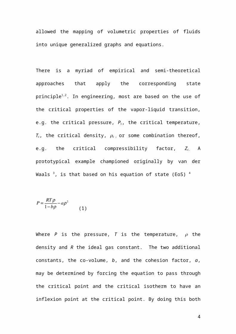
For a fixed set of (m, , ) a change in the repulsive exponent, increases the

acentric factor proportionally. As an illustration, Figure 5 shows the variation of the

repulsive exponent with the acentric factor for the case of a Mie spherical fluid (m =

1). From this figure, it is interesting to note that the limit of = 0 (a noble gas)

corresponds to an exponent of 14.8, reinforcing the idea that the choice of a (12-6)

potential to represent simple isotropic molecules is not optimal.

18

Figure 5 Repulsive exponent, , for a Mie (-6) spherical fluid (m = 1) as a

function of the acentric factor.

The linearity of the relationship between the Mie exponent and the acentric factor

suggests that one can correlate, by using a Padé series, the repulsive exponent:

(13)

The values of the parameters ai and bi are given in Table 1 for a single sphere (m = 1),

for dimer (m = 2), trimer (m = 3), tetramer (m = 4), pentamer (m = 5) and hexamer (m

= 6) molecules. The expression is valid for a repulsive range 9 < < 50 although the

smoothness of the curves allow for some degree of confidence in the extrapolation.

19

The very high values of the repulsive exponent will provoke premature freezing of the

fluid and the disappearance of the fluid phase region.

20

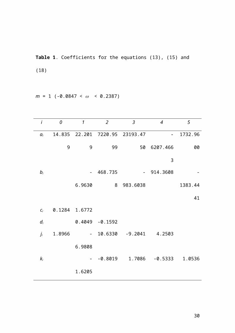
Table 1. Coefficients for the equations (13), (15) and (18)

m = 1 (-0.0847 < < 0.2387)

i 0 1 2 3 4 5

ai 14.8359 22.2019 7220.9599 23193.4750 -6207.4663 1732.9600

bi -6.9630 468.7358 -983.6038 914.3608 -1383.4441

ci 0.1284 1.6772

di 0.4049 -0.1592

ji 1.8966 -6.9808 10.6330 -9.2041 4.2503

ki -1.6205 -0.8019 1.7086 -0.5333 1.0536

m = 2 ( 0.0489 < < 0.5215)

i 0 1 2 3 4

ai 8.0034 -22.5111 3.5750 60.3129

bi -5.2669 10.2299 -6.4860

ci 0.1125 1.5404 -5.8769 5.2427

di -3.1954 2.5174 0.3518 -0.1654

ji -0.0696 -1.9440 6.2575 -5.4431 0.8731

ki -10.5646 25.4914 -20.5091 3.6753

21

m = 3 (0.1326 < < 0.7371)

i 0 1 2 3 4 5

ai 6.9829 -13.7097 -1.9604 17.3237

bi -3.8690 5.2519 -2.3637

ci -0.2092 4.2672 -9.7703 4.8661 -0.1950 4.2125

di -1.3778 -2.4836 3.5280 0.7918 -0.1246

ji 0.0656 -1.4630 3.6991 -2.5081

ki -8.9309 18.9584 -11.6668 -0.2561

m = 4 (0.2054 < < 0.9125)

i 0 1 2 3 4 5

ai 6.4159 -34.3656 59.6108 -21.6579 -35.8210 27.2358

bi -6.9751 19.2063 -26.0583 17.4222 -4.5757

ci 0.1350 1.3115 -10.1437 24.07292 -24.8084 9.7109

di -5.8540 13.3411 -14.3302 6.7309 -0.7830

ji 0.1025 -1.1948 2.8448 -1.9519

ki -8.1077 16.7865 -9.6354 -1.2390

m = 5 (0.1326 < < 0.7371)

22

i 0 1 2 3 4

ai 6.1284 -9.1568 -0.2229 4.5311

bi -2.8486 2.7828 -0.9030

ci 0.1107 1.9807 -6.6720 5.4841

di -3.1341 2.7657 -0.2737 -0.0431

ji 0.1108 -0.9900 2.2187 -1.5027

ki -7.3749 14.53173 -7.4967 -1.9209

m = 6 (0.3378 < < 1.1974)

i 0 1 2 3

ai 5.9217 -8.0711 0.4264 2.5560

bi -2.5291 2.1864 -0.6298

ci 0.1302 1.9357 -6.4591 5.1864

di -3.1078 2.8058 -0.4375

ji 0.2665 -0.4268 -0.2732 0.6486

ki 1.7499 -10.1370 9.4381

23

Upon fixing the repulsive exponent of the Mie potential (through the relation to the

acentric factor) a value of the van der Waals constant can be calculated from the

direct application of equation (9)

(14)

Once the range has been fixed, the corresponding (-6) fluid will have a unique

critical point, if expressed in terms of reduced properties. This critical can be

appropriately correlated with the van der Waals constant, , as they behave in a very

linear fashion ( c.f. figure 6).

24

Figure 6 Linear dependency of the reduced critical temperature for a

Mie (-6) spherical fluid (m = 1) as a function of van der Waals constant, .

Hence, the reduced critical temperature can be related to by means of a Padé series:

(15)

where the values of ci and di are given in Table 1. Furthermore, as for a given fluid the

critical coordinates (temperature, pressure, and density) and acentric factor are

commonly reported (see for example the databases described in refs. 38, 39, 40), so the

above equations allow the use of the critical temperature of a fluid to determine in a

25

direct fashion the corresponding energy scale of the associated Mie fluid. One only

needs to compare directly both the experimental critical temperature Tc of a real fluid

and the energy parameter of the Mie potential, as scaled by the Boltzmann constant

kB .

(16)

Similar correlations can be obtained for the other critical properties, such as the

critical pressure and density or compressibility factor. These could be employed to

obtain, in an analogous fashion as above, the corresponding link between properties of

real fluids and the size parameter, of the Mie fluid. Our experience has shown that

the values of obtained in this fashion would consistently underestimate (if were

regressed from critical pressure data) or overestimate (if were regressed from

critical density data) the saturated liquid densities. Scaling of the size parameter has a

clear relationship to the liquid density;

(17)

hence an alternative is to employ a parameter, similar in essence to the acentric factor,

i.e. the saturated liquid density at Tr = 0.70. Again, as before, we correlate the reduced

liquid density at Tr = 0.7 of the Mie fluids, , with the van der Waals constant α

26

by using the results obtained from the equation of state. The results can be

summarized in terms of a Padé series:

(18)

In eq. (18), ji and ki are coefficients given in Table 1 and Nav is Avogadro’s number.

corresponds to the experimental saturated liquid density at Tr = T/ Tc = 0.7

which may be obtained from common databases (32,33,34) and can be related to the

reduced property by means of equation (17).

As a summary and an explanation of the basic procedure we calculate here

intermolecular CG parameters for n-hexane. From the onset, a decision has to be

made to the level of coarse graining required and the number of beads, m, to be used

for representing the fluid. In view of the length-to breadth ratio of an extended hexane

molecule it is not unreasonable to describe it with a value of m = 2 (c.f. figure 4) . One

could, of course use other values, but the closer the ratio is to the real geometry, the

better the prediction of the model. Values that are too small (or too large) affect the

value of the repulsive exponent, tending to produce unrealistic potential parameters.

In practice, the inclusion of three backbone atoms in a CG bead seems to give the best

overall results.

The following “recipe” is suggested:

1) Fix a value of m. In the example, we use m = 2 for hexane

27

2) Using the experimental acentric factor one calculates the value of the

repulsive exponent using equation (13) and the constants in table 1

corresponding to the value of m. Taking = 0.299 34 one obtains = 19.26

3) Using equation (14) one obtains the value of the van der Waals constant . In

this case, = 0.6693

4) From eq. (15) and the constants in table 1 corresponding to the value of m one

obtains the reduced critical temperature for the Mie model. In the example

= 1.349.

5) This reduced property is compared to the experimental critical point to obtain

a scaling of the potential energy via equation (16). For hexane, a value of Tc =

507.82 K34 gives /kB = 376.35 K.

6) Similarly, the application of equation (18) gives a reduced density, of

for the corresponding Mie fluid. For = 0.6693 and m=2 one obtains

= 0.38466.

7) Finally, comparison of the above value with an experimental value of the

liquid phase density at a reduced temperature T/Tc =0.7 gives the size scale

of the model, through the use of equation (17). In this case, we seek the molar

density at a T = (0.7)(507.82)K = 355.47 K, which is found to be 34 =

6971.6 mol/m3 from which a value of = 4.508 Å is determined.

5. Molecular simulations employing the CG models

28

With the values of the potential found from the recipe described in the previous

section, one can perform CG molecular simulations to predict the thermophysical

properties of real fluids. Molecular dynamics (MD) simulation details are given in the

appendix A. They correspond to classical canonical MD runs where the liquid and the

vapour are both present in the simulation cell. By specifying the temperature and the

intermolecular potential parameters, one may obtain from these particular simulations

a prediction of the coexisting equilibrium densities, the vapour pressure and the

surface tension of the system. Following the example given above, for n-hexane it can

be modelled as a tangent dimer with a (19.26-6) Mie potential, with /kB = 376.35 K

and = 4.508 Å. In figure 7 we plot the temperature-density plot obtained both from

MD simulations as compared to the smoothed experimental data. One can observe

that the prediction of the correlation is excellent. A minor deviation in the vapour

pressure is observed in figure 8 for the same system and this is related to the inability

of the equation of state of simultaneously fitting both subcritical properties and

critical points. In addition, we present in figure 7 the results calculated from SAFT-

using the same parameter values The curves calculated with the SAFT- EoS are

presented for comparison purposes only and exemplify the close agreement between

the theory and the simulations results, a sine qua non condition for employing a

methodology as the one proposed herein.

Figure 9 exemplifies the real potential use of the correlation, as the force field can be

used for molecular simulations of properties not considered in the original

parametrization, for example surface properties and interfacial tensions. Here, the

equation of state is not amenable to be used, unless a more sophisticated theory is

29

employed 41,42. However the simulations provide an accurate prediction of the

interfacial properties over the full temperature range. Analysis of the simulations

would also provide interfacial profiles, and structure correlations for the

inhomogeneous fluid. Similarly, other interfacial properties such as adsorption could

be studied.

Figure 7 Temperature, T, as a function of molar density , for n-hexane.

Solid line corresponds to the smoothed experimental data40 dashed lines are

the description from the SAFT- equation of state. Solid symbols are MD

simulation data. In both the EOS and the simulations the Mie (-6) model

parameters ( = 19.26, /kB = 376.35 K, = 4.508 Å) are obtained from the

correlation with m taken as 2.

30

Figure 8 Vapor pressure P, as a function of temperature, T, for n-hexane.

Symbols as in figure 7

31

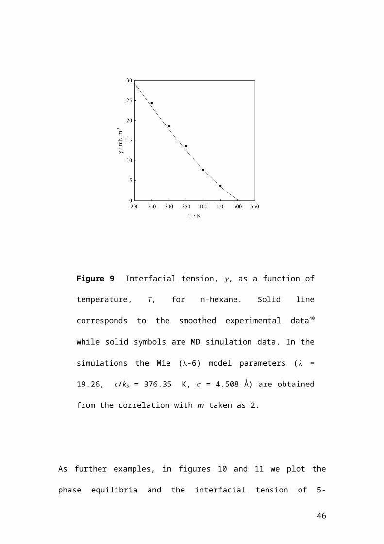
Figure 9 Interfacial tension, , as a function of temperature, T, for n-

hexane. Solid line corresponds to the smoothed experimental data40 while

solid symbols are MD simulation data. In the simulations the Mie (-6)

model parameters ( = 19.26, /kB = 376.35 K, = 4.508 Å) are obtained

from the correlation with m taken as 2.

As further examples, in figures 10 and 11 we plot the phase equilibria and the

interfacial tension of 5-nonanone (C9H18O). This molecule is an example of a non-

trivial polar elongated molecule. Here, the acentric factor is capturing both the effects

of polarity and elongation. If we choose to model the fluid as a trimer ( m = 3) we

effectively decouple both effects. The correlation in equation (13) gives then the

exponent of each of the three beads that averages out the polar contribution. The

quality of the prediction made by the molecular simulation of the CG model for both

32

the phase diagram, vapour pressure (not shown) and the interfacial tension is

excellent.

Figure 10 Temperature, T, as a function of molar density , for for C9H18O

( 5-nonanone). Solid line corresponds to the smoothed experimental data40

dashed lines are the description from the SAFT- equation of state. Solid

symbols are MD simulation data. In both the EOS and the simulations the

Mie (-6) model parameters ( = 22.72, /kB = 445.81 K, = 4.433 Å) are

obtained from the correlation with m is taken as 3.

33

Figure 11 Interfacial tension, , as a function of temperature, T, for C9H18O

(5-Nonanone). Solid line corresponds to the smoothed experimental data40

while solid symbols are MD simulation data. In the simulations the Mie (-

6) model parameters ( = 22.72, /kB = 445.81 K, = 4.433 Å) are

obtained from the correlation with m taken as 3.

The CG potentials presented here are effective force fields that offer an appropriate

average of the volumetric properties, as expressed in a phase diagram.

Notwithstanding the simplifications, these potentials provide a representation that is

of similar quality as that delivered by more detailed atomistic models. In figure 12 we

34

show the prediction for eicosane ( C20H42 ), a long chain n-alkane, along with the

simulation results for a detailed atomistic model38. Given the uncertainty of the

experimental results, the simulations show a remarkable agreement with both

experiments and more sophisticated force fields. We have used the critical data

suggested in ref. 33 ( = 0.906878, Tc = 768 K, = 2188.388   mol/m3). In this

particular case, the model parameters depend on the values of the critical temperature

of this fluid, which can not be measured, as eicosane would decompose before

reaching the critical region.

35

Figure 12 Temperature, T, as a function of molar density , for n-C20H42

with m = 6. Solid line corresponds to the smoothed experimental data40,

symbols are MD simulation data for a) detailed united atom potentials (38)

open circles, and b) and for the CG Mie (-6) model full circles with

parameters ( = 24.70, /kB = 453.10 K, = 4.487 Å) obtained from the

correlation.

There is nothing in the SAFT theory that restricts the use of the potentials to pure

fluids, however, no attempt has been made here to consider mixtures. The most

crucial aspect of the description of mixtures is the determination of the cross

parameters between unlike beads. Ideally, these should be determined from mixture

data. In lieu of any information, simple combining rules can be applied, e.g.

(18a)

(18b)

(18c)

where the subscripts A and B refer to the individual components of the mixture.

The correlations in the previous section assume that the intermolecular potential is

isotropic in nature and has a simple repulsion-dispersion interaction that can be

36

mapped into a Mie potential. When used within the framework of coarse-grained

modelling, such assumptions might break down, e.g. the modelling of a complexly

bonded group of atoms or the presence of delocalized charges with subsequent

formation of hydrogen bonds. In these cases, the models presented here can only be

taken as first guesses and crude approximations. Consider, for example the case of

water. Clearly coarse graining using a simple isotropic sphere is far from reality.

Notwithstanding, many attempts to parametrize water at this level of coarse graining

have been made43. Water has an abnormally large acentric factor which is caused by

the relatively strong intermolecular attractions brought by the presence of the

hydrogen bonding network formed in the liquid phase. If one attempts to use the

recipe given in this paper to water, an immediate observation is that it suggests the use

of a very large repulsive exponent. In terms of the correlation, this high acentric factor

suggests the use of an unrealistically large value for the repulsive exponent. While

this procedure will force the system to have a sensible values of the vapor pressure,

other properties will be poorly represented. Particularly, the very high values of the

repulsive exponent induce the freezing of the model at temperatures above those

expected, rendering the model unsuitable for fluid phase modelling. This is a classical

example where coarse graining techniques struggle to give satisfactory results. In the

case of water, the premature freezing may be avoided by considering a different

approach for determining the value of that should be used in the correlations. The

fluid phase region of the Mie spherical fluid is determined by the value of through a

simple relationship18 between the critical and triple points; Tc/Tt = 1.464 + 0.608.

This allows one to use a different value of alpha ( = 1.203) and a corresponding

value of the repulsive exponent through equation (14), the former being compatible

with maintaining the fluid phase region. The rest of the procedure, i.e. fitting the

37

depth of the potential with the critical temperature and the size parameter with a

density follows in the usual fashion. The full set of parameters for this simple model

of water correspond to a (8.4-6) potential with /kB = 378.87 K ; = 2.915 Å and

represent a sensible compromise for the prediction of fluid properties of water with an

isotropic, temperature independent model. Reassuringly, it resembles other models of

water obtained by heroic parametric force fitting efforts of water data to

thermophysical properties44.

The data points needed for each molecule are the acentric factor, the critical

temperature and the liquid density at the reduced temperature of 0.7. One of course,

can envision scenarios where this particular piece of information is absent, in

particular the latter. In such cases we suggest the density to be calculated from a

suitable correlation such as the Rackett model 45

(17)

although many other options are available46 and could equivalently be employed. The

quality of the potentials obtained is decreased, in expense of the universality of the

method. A table of parameters for over 7000 organic compounds is available from the

authors. No attempt has been made to be exhaustive, and the compilation is presented

as an example of the breadth and depth of the proposed method. It includes not only

simple fluids, but refrigerants and polar compounds, elongated molecules and general

fluids of industrial interest.

38

In the case of chain molecules the intramolecular interactions must additionally be

defined. Following the SAFT treatment, all pairs of beads are assumed to be bonded

at a distance corresponding to The nature of the bond is rigid, although a

harmonic spring with a large constant is equivalent. For molecules consisting of three

or more beads, an issue arises with respect to the geometry or bonding angle of the

molecule. Wertheim’s first order thermodynamic perturbation theory, which underlies

the SAFT treatments, only considers bonding between pairs of molecules and makes

an assumption that any further bonding on a bead is independent of the existing

bonds. The practical consequence of this is that the theory is more accurate for

stretched out chains47. In most cases a fully flexible model will suffice, but an

improved mapping between simulation and theory is achieved if a bending potential is

added between trios of beads as to favour the linear configuration.

6. Conclusion

The corresponding states principle is not a physical law, but rather a handle to

understand and correlate in a systematic way the behaviour of simple fluids. Modern

corresponding states correlations for the description of thermophysical properties of

fluids are based on the assumption that there is an underlying (and universal) function

that can describe the intermolecular potential of said fluids. Following such a

postulate, statistical mechanics treatments allow the calculation of the properties of a

particular fluid. Most interestingly, the results may be generalized if they are scaled

appropriately. The number of independent scales employed, dictates the way the

39

fluids can be mapped into such a “universal” function. We have employed here the

premise that most simple non-associating fluids may be well described by an

intermolecular potential of the Mie type and molecules described as linear chains of

said spheres. This representation of a fluid, in terms of four scales (m, , ) is

the basis, facilitated by the SAFT- EOS, of the proposed four parameter

corresponding state correlation. The unique element of this correlation is that the

parameters obtained can be directly employed in molecular simulation of fluids with

no loss in accuracy and as such are comparable to more detailed atomistic models.

The procedure described herein is a top-down approach (also called thermodynamic

approach) to the development of force fields. In its more accurate implementation,

one would use the EOS to fit the available volumetric experimental data of a fluid,

hence obtaining an effective average force field. Intramolecular interactions could

also be obtained from first principles simulations to complete the description of the

potential. Such an approach is very effective and has been used in a variety of

scenarios to predict by simulation the behaviour of complex fluids such as liquid

crystals, surfactants, and polymers 40. The correlation presented here is a short-cut of

the aforementioned philosophy, and allows the determination in a very fast and

effective way of intermolecular force field parameters that can be used in efficient

computational schemes.

40

References

41

1 () Hirschfelder, J. O.; Curtiss, C. F.; Bird, R. B. Molecular Theory of Liquids and Gases;

Wiley: New York, 1965.

2 () Reed, T. M.; Gubbins, K. E. Applied Statistical Mechanics; McGraw-Hill: New York,

1973.

3 () van der Waals, J. D. Onderzoekingen Omtrent de Overeenstemmende Eigenschappen der

Normale Verzadigden-Damp - en Vloeistoflijnen Voor de Verschillende Stoffen en Omtrent

een Wijziging in Den Vorm Dier Lijnen Bij Mengsels [Investigations on the Corresponding

Properties of the Normal Saturated Vapor and Liquid Curves for Different Fluids, and About

A Modification in the Form of These Curves for Mixtures]. Verhand. Kon. Akad. Wetensch.

Amst. 1880, 20, 1.; Over de Coëfficiënten van Uitzetting en van Samendrukking in

Overeenstemmende Toestanden der Verschillende Vloeistoffen [On the Coefficients of

Expansion and Compression in Corresponding States of Different Liquids]. Verhand. Kon.

Akad. Wetensch. Amst. 1880, 20, 1.

4 () van der Waals, J. D. Over de Continuiteit Van Den Gas- En Vloeistoftoestand. Ph.D.

Dissertation, University of Leiden, Leiden, 1873.

5 () Vera, J. H.; Prausnitz, J. M. Generalized van der Waals Theory for Dense Fluids. Chem.

Eng. J. 1972, 3, 1.

6 () Widom, B. Statistical Mechanics: A Concise Introduction for Chemists; Cambridge

University Press: Cambridge, 2002.

7 () Soave, G. Equilibrium Constants From a Modified Redlich – Kwong Equation of State.

Chem. Eng. Sci. 1972, 27, 1197.

8 () Pitzer, K. S.; Lippman, D. Z.; Curl, R. F.; Huggins, C. M.; Petersen, D. E. The Volumetric

and Thermodynamic Properties of Fluids. II. Compressibility Factor, Vapor Pressure and

Entropy of Vaporization 1. J. Am. Chem. Soc. 1955, 77, 3433.

9 () Bett, K. E.; Rowlinson, J. S.; Saville, G. Thermodynamics for Chemical Engineers;

Athlone Press:, 1975.

10 () Prausnitz, J. M.; Lichtenthaler, R. N.; Gomes de Azevedo, E. Molecular Thermodynamics

of Fluid-Phase Equilibria; 3rd Edition, Prentice Hall: New Jersey, 1998.

11 () Assael, M. J.; Trusler, J. P. M.; Tsolakis, T. F. Thermophysical Properties of Fluids;

Imperial College Press: London, 1996.

12 () Xiang, H. The Corresponding-States Principle and its Practice; Elsevier: Amsterdam,

2005.

13 () Jones, J. E. On the Determination of Molecular Fields. II. From the Equation of State of a

Gas. Proc. R. Soc. Lon. A. 1924, 106, 463.

14 () Mie, G. Zur kinetischen Theorie der Einatomigen Körper. Ann. Phys. 1903, 316, 657.

15 () Grüneisen, E. A. Theorie des Festen Zustandes Einatomiger Elemente Ann. Phys. 1912,

344, 257.

16 () Lennard-Jones, J. E. Wave Functions of Many-Electron Atoms. Proc. Phys. Soc. 1931,

27, 469.

17 () Gil-Villegas, A.; Galindo, A.; Whitehead, P. J.; Mills, S. J.; Jackson, G.; Burgess, A. N.

Statistical Associating Fluid Theory for Chain Molecules with Attractive Potentials of

Variable Range. J. Chem. Phys. 1997, 106, 4168.

18 () Ramrattan, N. Simulation and Theoretical Perspectives of the Phase Behaviour of Solids,

Liquids and Gases Using the Mie Family of Intermolecular Potentials. Ph.D. Dissertation,

Imperial College London, London, 2013.

19 () Kulinskii, V. L. The Vliegenthart-Lekkerkerker Relation: The Case of the Mie-Fluids. J.

Chem. Phys. 2011, 134, 144111.

20 () Müller, E. A.; Gubbins, K. E. Molecular-Based Equations of State for Associating Fluids:

A Review of SAFT and Related Approaches. Ind. Eng. Chem. Res. 2001, 40, 2193.

21 () Economou, I. G. Statistical Associating Fluid Theory: A Successful Model for the

Calculation of Thermodynamic and Phase Equilibrium Properties of Complex Fluid

Mixtures. Ind. Eng. Chem. Res. 2002, 41, 953.

22 () Tan, S. P.; Adidharma, H.; Radosz, M. Recent Advances and Applications of Statistical

Associating Fluid Theory. Ind. Eng. Chem. Res. 2008, 47, 8063.

23 () McCabe, C.; Galindo, A. SAFT associating fluids and fluid mixtures. In Applied

Thermodynamics of Fluids; Goodwin, A. R., Sengers, J., Peters, C. J., Eds.; Royal Society of

Chemistry: London, 2010, Chapter 8.

24 () Papaioannou, V.; Lafitte, T.; Avendaño, C.; Adjiman, C. S.; Jackson, G.; Müller, E. A.;

Galindo. A. Group Contribution Methodology Based on the Statistical Associating Fluid

Theory for Heteronuclear Molecules Formed From Mie Segments. J. Chem. Phys. 2014,140,

054107

25 () Lafitte, T.; Apostolakou, A.; Avendaño, C.; Galindo, A.; Adjiman, C. S.; Müller, E. A.;

Jackson, G. Accurate Statistical Associating Fluid Theory for Chains of Mie Segments. J.

Chem. Phys. 2013, 139, 154504.

26 () Avendaño, C.; Lafitte, T.; Galindo, A.; Adjiman, C. S.; Jackson, G.; Müller, E. A. SAFT-γ

Force Field for the Simulation of Molecular Fluids. 1. A Single-Site Coarse Grained Model

of Carbon Dioxide. J. Phys. Chem. B 2011, 115, 11154.

27 () Avendaño, C.; Lafitte, T.; Adjiman, C. S.; Galindo, A.; Müller, E. A.; Jackson, G. SAFT-γ

Force Field for the Simulation of Molecular Fluids: 2. Coarse-Grained Models of

Greenhouse Gases, Refrigerants, and Long Alkanes. J. Phys. Chem. B 2013, 117, 2717.

28 () Müller, E. A.; Gubbins, K. E. An Equation of State for Water From A Simplified

Intermolecular Potential. Ind. Eng. Chem. Res. 1995, 34, 3662.

29 () Cuadros, F.; Cachadiña, I.; Ahumada, W. Determination of Lennard- Jones Interaction

Parameters Using A New Procedure. Mol. Eng. 1996, 6, 319.

30 () Ben-Amotz, D.; Gift, A. D.; Levine, R. D. Improved Corresponding States Scaling of the

Equations of State of Simple Fluids. J. Chem. Phys. 2002, 117, 4632.

31 () Lotfi, A.; Vrabec, J.; Fischer, J. Vapor-Liquid-Equilibria of the Lennard-Jones Fluid from

the NPT Plus Test Particle Method. J. Mol. Phys. 1992, 76, 1319.

32 () Stoll, J.; Vrabec, J.; Hasse, H.; Fischer, J. Comprehensive Study of the Vapour-Liquid

Equilibria of the Pure Two-Centre Lennard-Jones Plus Point Quadrupole Fluid. Fluid Phase

Equilib. 2001, 179, 339.

33 () Vrabec, J.; Stoll, J.; Hasse, H. A Set of Molecular Models for Symmetric Quadrupolar

Fluids. J. Phys. Chem. B 2001, 105,12126

34 () Stoll, J.; Vrabec, J.; Hasse, H. Comprehensive Study of the Vapour-Liquid Equilibria of

the Two-Centre Lennard-Jones Plus Point Dipole Fluid. Fluid Phase Equilib. 2003, 209, 29.

35 () Vrabec, J.; Huang, Y.-L.; Hasse, H. Molecular Models for 267 Binary Mixtures Validated

by Vapor-Liquid Equilibria: A Systematic Approach. Fluid Phase Equilib. 2009, 279, 120.

36 () Müller, E. A.; Jackson, G. Force Field Parameters from the SAFT-γ Equation of State for

Use in Coarse-Grained Molecular Simulations. Ann. Rev. Chem. Biomol. Eng. 2014, in

press, doi: 10.1146/annurev-chembioeng-061312-103314

37 () Tester, J. W.; Modell, M. Thermodynamics and its Applications; 3rd Ed. Prentice Hall:

New Jersey, 1997.

38 () Daubert, T. E.; Danner, R. P. Physical and Thermodynamic Properties of Pure Chemicals.

Data Compilation; Taylor and Francis: Bristol, PA, 1989.

39 () DECHEMA Gesellschaft für Chemische Technik und Biotechnologie e.V., Frankfurt am

Main, Germany, https://cdsdt.dl.ac.uk/detherm/ (retrieved November, 2013).

40 () Lemmon, E. W.; McLinden, M. O.; Friend, D. G. Thermophysical Properties of Fluid

Systems in NIST Chemistry WebBook, NIST Standard Reference Database Number 69;

Linstrom, P. J., Mallard, W. G., Eds.; National Institute of Standards and Technology:

Gaithersburg MD; http://webbook.nist.gov (retrieved November, 2013).

41 () Müller, E. A.; Mejía, A. Interfacial Properties of Selected Binary Mixtures Containing n-

Alkanes. Fluid Phase Equilib. 2009, 282, 68.

42 () Müller, E. A.; Mejía, A. Comparison of United-Atom Potentials for the Simulation of

Vapor-Liquid Equilibria and Interfacial Properties of Long-Chain n-Alkanes up to n-C100.

J. Phys. Chem. B 2011, 115, 12822.

43 () Lobanova, O.; Avendaño, C.; Lafitte, T.; Jackson, G.; Müller, E.A. SAFT-γ Force Field

for the Simulation of Molecular Fluids. 4. A Single-Site Coarse Grained Model of Water

Valid Over a Wide Temperature Range. Mol Phys. Submitted.

44 () He, X. B.; Shinoda, W.; DeVane, R.; Klein, M. L. Exploring the Utility of Coarse-Grained

Water Models for Computational Studies of Interfacial Systems. Mol. Phys. 2010, 108,

2007.

45 () Rackett, H. G. Equation of State for Saturated Liquids. J. Chem. Eng. Data 1970, 15, 514.

46 () Mulero, A.; Cachadiña, I.; Parra, M. I. Liquid Saturation Density from Predictive

Correlations Based on the Corresponding States Principle. Part 1: Results for 30 Families of

Fluids. Ind. Eng. Chem. Res. 2006, 45, 1840.

47 () Müller, E. A.; Gubbins, K. E.; Simulation of Hard Triatomic and Tetratomic Molecules. A

Test of Associating Fluid Theories. Mol. Phys. 1993, 80, 957.

Acknowledgment

This paper is dedicated to the 40 years of academic career of Prof. Claudio Olivera-Fuentes, a

pioneer in equation of state development, whose ideas have inspired the paths of all three authors.

The authors gratefully acknowledge the many fruitful discussions with the members of Imperial

College’s Molecular Systems Engineering group and in particular with Prof. George Jackson, Dr.

Carlos Avendaño and Dr. Thomas Lafitte. The efforts of two exceptional undergraduate students,

Karson Wong and Muhammad Jansi who compiled some of the published test data is much

appreciated. This work was financed by FONDECYT, Chile (Project 1120228) and supported by

the U.K. Engineering and Physical Sciences Research Council (EPSRC) through research grants

(EP/I018212 and EP/J014958). Simulations described herein were performed using the facilities of

the Imperial College High Performance Computing Service.

Supporting Information Available: Supporting Information S1: Molecular Dynamics Simulation

details, This information is available free of charge via the Internet at http: //pubs.acs.org.

Figure Captions

Figure 1 : Temperature, T – density, , phase diagram of an attractive sphere (solid line) and

the corresponding trimer (dashed-dotted) oligomer formed by spheres of the same type.

Figure 2 Effect of intermolecular interactions on the slope of the vapor pressure curve. The

ordinate corresponds to the base 10 log of the ratio of the vapor pressure to the critical point

(corresponding to -1-. For the noble gases this takes on the value of zero, and becomes

larger as the interaction deviates either because of non-sphericity (e.g. n-C10H22) and/or as a

consequence of deviations from simple dispersive interactions (e.g. CF4)

Figure 3 Conformality of the Mie potential. Phase behaviour of a LJ (12-6) potential (solid line)

as compared to the Mie (14-7) (dashed line) where the ratio r ais kept the same as the LJ

and the Mie (9.159-7) (dashed-dotted) where the van der Waals constant , is kept the same as

the LJ potential. In all cases the parameters, (, are kept equal. Top is the temperature, T

– density, , diagram, bottom is the vapour pressure curve.

Figure 4 Coarse graining of a simple fluid. A molecule of n-hexane is rendered as a dimer (m

=2) composed of twin tangent spheres, each described via a Mie potentials with size , and

energy parameters and a van der Waals constant describing the range or form of the

potential. No geometric or bottom-up mapping is employed.

Figure 5 Repulsive exponent, , for a Mie (-6) spherical fluid (m = 1) as a function of the

acentric factor.

Figure 6 Linear dependency of the reduced critical temperature for a Mie (-6) spherical

fluid (m = 1) as a function of van der Waals constant, .

Figure 7 Temperature, T, as a function of molar density , for n-hexane. Solid line

corresponds to the smoothed experimental data40 dashed lines are the description from the

SAFT- equation of state. Solid symbols are MD

Figure 8 Vapor pressure P, as a function of temperature, T, for n-hexane. Symbols as in figure

7

Figure 9 Interfacial tension, , as a function of temperature, T, for n-hexane. Solid line

corresponds to the smoothed experimental data40 while solid symbols are MD simulation data.

In the simulations the Mie (-6) model parameters ( = 19.26, /kB = 376.35 K, = 4.508 Å)

are obtained from the correlation with m taken as 2.

Figure 10 Temperature, T, as a function of molar density , for for C9H18O ( 5-nonanone).

Solid line corresponds to the smoothed experimental data40 dashed lines are the description from

the SAFT- equation of state. Solid symbols are MD simulation data. In both the EOS and the

simulations the Mie (-6) model parameters ( = 22.72, /kB = 445.81 K, = 4.433 Å) are

obtained from the correlation with m is taken as 3.

Figure 11 Interfacial tension, , as a function of temperature, T, for C9H18O (5-Nonanone).

Solid line corresponds to the smoothed experimental data40 while solid symbols are MD

simulation data. In the simulations the Mie (-6) model parameters ( = 22.72, /kB = 445.81

K, = 4.433 Å) are obtained from the correlation with m taken as 3.

Figure 12 Temperature, T, as a function of molar density , for n-C20H42 with m = 6. Solid line

corresponds to the smoothed experimental data40, symbols are MD simulation data for a)

detailed united atom potentials (38) open circles, and b) and for the CG Mie (-6) model full

circles with parameters ( = 24.70, /kB = 453.10 K, = 4.487 Å) obtained from the

correlation.

For Table of Contents only