The method of modeling the human EEG by calculating radial ... · left hemisphere of the cortical...

The method of modeling the human EEG by calculating radial

traveling waves on the folded surface

of the human cerebral cortex

Vitaly M. Verkhlyutov, Vladislav V. Balaev

Institute of Higher Nervous Activity & Neurophysiology of RAS, Moscow

Address correspondence to:

Dr. Vitaly Verkhlyutov

Institute of Higher Nervous Activity & Neurophysiology of RAS

5A, Butlerova St., Moscow 117485, Russia

Phone/Fax: +7 499-743-00-56

E-mail: [email protected]

All rights reserved. No reuse allowed without permission. (which was not peer-reviewed) is the author/funder, who has granted bioRxiv a license to display the preprint in perpetuity.

The copyright holder for this preprint. http://dx.doi.org/10.1101/242412doi: bioRxiv preprint first posted online Jan. 4, 2018;

http://dx.doi.org/10.1101/242412

2

Abstract There are many data about traveling waves in the cortex of animals such as

rats, ferrets, monkey, and even birds. Waves registered invasively using electrical

and optical imaging techniques. Such registration is not possible in healthy man.

Non-invasive EEG recordings show scalp waves propagation at rates two

orders greater than the data obtained invasively in animal experiments. At the same

time, it has recently been argued that the traveling waves of both local and global

nature do exist in the human cortex. We have developed a novel methodology for

simulation of EEG as produced by depolarization waves with parameters taken

from animal models. We simulate radially propagating waves, taking into account

the complex geometry of the surface of the gyri and sulci in the areas of the visual,

motor, somatosensory and auditory cortex. The dynamics of the distribution of

electrical fields on the scalp in our simulations is consistent with the EEG data

recorded in humans.



http://dx.doi.org/10.1101/242412

3

Introduction

Traveling waves (TW) on the cerebral cortex surface were discovered in the

30s of the 20th century (Adrian & Mathews, 1934), and were then detected in

human via the EEG mapping (Adrian & Yamagiva, 1935; Lindsley, 1938) and then

were investigated minutely in 50-60s (Walter, 1953; Petsche, 1955; Shipton, 1957;

Anan’iev et al., 1956; Livanov & Anan’iev, 1960, Monakhov, 1961; Dubikaitis

and Dubikaitis, 1960, Raimond, 1961) and less intensively in subsequent years

(Hughes, 1995). At present, interest in this phenomenon returned for reasons the

registration techniques improvement (Ferrea, 2012) and owing to a number of

physiological discoveries (Biswal et al., 1995; Hindriks et al., 2014; Matsui et al.,

2016), which may explain of the TW.

TW on the surface of the scalp have a speed of about 5-15 m/s (Alexander et

al., 2013), while lower speed was recorded in electrocorticography (ECoG)

experiments (Zhang et al., 2017). Moreover, when recorded using microelectrode

matrices placed on the cortical surface, the velocity of the TW appeared lower than

0.5 m/s (Martinet et al., 2017) which is similar to the speed detected in animals by

means of electrical (Rubino et al., 2006; Ferezou et al., 2007; Reimer et al. al.,

2011; Takahashi et al., 2011) or optical recordings (Muller et al., 2014).

Importantly, when registered within a small area about 16 mm2, simpler TW

configurations appear, which in many cases might be interpreted as radial waves

propagating from one epicenter (Martinet et al., 2017).

Previously, we proposed an elementary model for the TW spread within the

human visual cortex, which explained all known to us at that time phenomena of

EEG TW in alpha-range on the head (Verkhliutov, 1996). However, the

primitiveness of this model made it necessary to search ways of calculating TW in

a more realistic model. This became possible when the appearance of the

Boundary Element Method (BEM) based on the high quality MRI images (Fuchs



http://dx.doi.org/10.1101/242412

4

et al., 1998) and algorithms for geodetic distances calculation on complex surfaces

(Siek et al. 2002).

In this report we propose an EEG data generatin method consistent with the

intracortical hypothesis (Hindriks, 2014), which suggests that the main activity

recorded in the EEG is related to the TWs of electrical potentials propagated by

intra-cortical short fibers (Ermentrout & Kleinfeld, 2001; Han et al., 2008 ; Zheng

& Yao, 2012). We limit our attention to only radially propagating omni-directional

waves in the 10 Hz range.

We also assume that spontaneous TWs are not a constant process on the

cortex surface and we believe that TW are more related to rest, sleep, pathological

and epileptic activity (Wu et al., 2008). The spontaneous TWs are suppressed

during sensory stimulation (Muller et al., 2014). At the same time the evoked and

motor potentials exhibit TW-like nature (Rubino et al., 2006).



http://dx.doi.org/10.1101/242412

5

Results

Dynamic distributions of dipoles (Fig.2C) from concentrically propagating

potential waves (Fig 2D, 3C) from 28 epicenters located at various cortical points

(Fig. 1) were calculated. We simulated 28 128-channel EEG tracks (Fig.2A, 3A &

Supplementary materials) and calculated the distribution of EEG potentials on the

scalp (Fig. 2B; 3B & Supplementary materials). In all of the cases the standard

localization methods did not manage to reproduce the wave-like potential

distribution on the cortical surface (Fig. 3D & Supplementary materials). We also

reproduced traveling waves on the scalp (see Supplementary materials).

Table 1 summarizes the data: the epicenters of modeled waves, the

anatomical structures their pertain to, the functional cortical networks in which the

wave process is assumed to propagate, the EEG rhythms, the maximum given

current density in the cortex, the maximum potential amplitude on the scalp

surface, dynamics of the distribution of potentials on the surface of the scalp.

The models of alpha rhythm and alpha-like rhythms differed in localization

only. The epicenters for the alpha rhythm were placed in the regions of the

calcarinus and parieto-occipital sulcuses, the ones for the mu-rhythm placed in the

area of the central sulcus, and for the tau rhythm, the epicenters were set in the

vicinity of the Silvian fissure.

With an equal wave source current density of ± 50 nA / mm2 in the cortex,

the potential amplitudes on the scalp were greatest for the alpha rhythm reaching

160 µV from peak to peak. The same value for the mu-rhythm was 110 µV, and 90

µV for the tau rhythm. Such values agree with those observed experimentally for

these rhythms (Markand.,1990).

The most frequent dynamics is TW from frontal to occipital lobe - 10

epicenters out of 14 are observed for alpha sources. The total amplitude in this case

was 802 µV. For TW from the occipital to the frontal regions - 290 µV.

TWs from the frontal to the occipital lobe and in the opposite direction for

mu-and tau-rhythms are approximately equal for different epicenters. In most



http://dx.doi.org/10.1101/242412

6

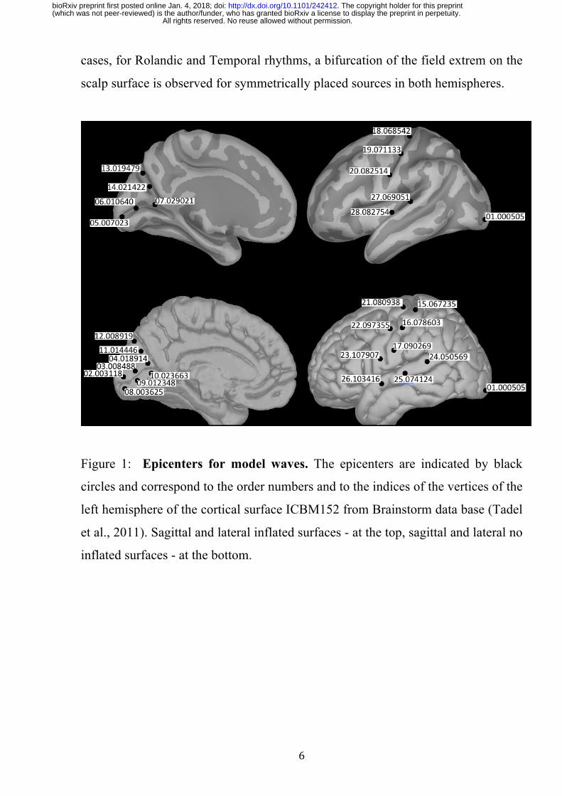
cases, for Rolandic and Temporal rhythms, a bifurcation of the field extrem on the

scalp surface is observed for symmetrically placed sources in both hemispheres.

Figure 1: Epicenters for model waves. The epicenters are indicated by black

circles and correspond to the order numbers and to the indices of the vertices of the

left hemisphere of the cortical surface ICBM152 from Brainstorm data base (Tadel

et al., 2011). Sagittal and lateral inflated surfaces - at the top, sagittal and lateral no

inflated surfaces - at the bottom.



http://dx.doi.org/10.1101/242412

7

Figure 2: Modeling the EEG from a radial wave in the visual cortex. (A) 100 ms of simulated EEG , (B) electric field distribution on the “scalp” from two symmetric waves in both hemispheres with an epicenter at the vertex 04.18914 of the cortical surface model ICBN152 (the second wave is mirrored with respect to the sagittal plane), (C) the equivalent dipole corresponding to the time moment marked by the cursor in (A), (D) the current density distribution from model radial wave on the cortical surface.



http://dx.doi.org/10.1101/242412

8

Figure 3: Modeled EEG from the wave propagation of potentials with the epicenter at the occipital pole. (A) Modeled EEG for 100 ms. (B) Electric field distribution on the “scalp” from wave in left hemisphere with an epicenter at the vertex 01.000505 of the cortical surface model ICBN152. (C) The current density distribution from radial wave on the cortical surface model. (D) The current density distribution on the “cortex” localized by the wMNE standard method.



http://dx.doi.org/10.1101/242412

9

Table 1. The maximum amplitude of the modeled EEG and the type of moving waves on the scalp from radial waves propagating from the epicenters located in the visual, sensorimotor and auditory cortex of the human brain's ICBN152 model. № Vertex MNI Structure RSN Rhythm CD SPL STWL SPB STWB

1 01.000505 -18.8 -102.7 -3.2 Pol.occipital. VIS alpha ±50 ±40 RL ±50 2OF 2 04.018914 -0.0 -73.3 15.3 Cuneus VIS alpha ±50 ±20 RR ±40 FO 3 03.008488 0.5 -84.4 7.3 Cuneus VIS alpha ±50 ±25 L ±45 OF 4 02.003118 0.6 -93.8 2.6 Cuneus VIS alpha ±50 ±40 RR ±80 FO 5 11.014446 0.4 -76.9 24.4 Cuneus VIS alpha ±50 ±45 RR ±80 FO 6 12.008919 -0.0 -83.2 34.1 Cuneus VIS alpha ±50 ±15 RR ±30 FO 7 10.023663 -0.9 -66.8 3.0 G.lingualis VIS alpha ±50 ±20 RA ±30 OF 8 09.012348 -0.0 -80.2 -2.1 G.occ.temp. VIS alpha ±50 ±20 R ±35 OF 9 08.003625 -0.6 -93.0 -10.7 G.occ.temp. VIS alpha ±50 ±20 OF ±35 OF

10 07.029021 -28.1 -62.8 5.7 S.calcarinus VIS alpha ±50 ±7 RP ±9 2FO 11 06.010640 -12.3 -80.5 4.2 S.calcarinus VIS alpha ±50 ±20 L ±7 FO 12 05.007023 -4.5 -87.7 -0.8 S.calcarinus VIS alpha ±50 ±15 RR ±30 OF 13 14.021422 -15.4 -68.5 26.5 S.p.occip. VIS alpha ±50 ±20 RP ±40 FO 14 13.019479 -14.6 -71.3 34.7 S.p.occip. VIS alpha ±50 ±20 RP ±35 FO 15 15.067235 -47.6 -28.9 64.0 G.postcentr. SSM mu ±50 ±15 RL ±15 2FO 16 16.078603 -59.1 -18.8 49.3 G.postcentr. SSM mu ±50 ±15 LP ±25 2FO 17 17.090269 -65.6 -9.9 25.3 G.postcentr. SSM mu ±50 ±25 L ±30 2OF 18 21.080938 -37.8 -17.3 69.7 G.precentr. SSM mu ±50 ±15 RP ±25 FO 19 22.097355 -56.2 -4.6 47.6 G.precentr. SSM mu ±50 ±25 RR ±25 2OF 20 23.107907 -62.4 4.3 20.3 G.precentr. SSM mu ±50 ±20 RL ±20 2OF 21 18.068542 -22.0 -27.4 55.1 S.Rolandic SSM mu ±50 ±30 RP ±55 2FO 22 19.071133 -34.4 -25.7 49.3 S.Rolandic SSM mu ±50 ±30 FO ±50 FO 23 20.082514 -41.8 -15.7 33.7 S.Rolandic SSM mu ±50 ±40 RA ±30 2OF 24 24.050569 -67.1 -41.3 14.8 G.temp.sup. AUD tau ±50 ±15 R ±20 2OF 25 25.074124 -67.9 -23.1 4.9 G.temp.sup. AUD tau ±50 ±15 RR ±25 2FO 26 26.103416 -61.0 0.6 -7.1 G.temp.sup. AUD tau ±50 ±25 RR ±30 2FO 27 27.069051 -61.0 0.6 -7.1 F.Sylvian AUD tau ±50 ±25 L ±40 2OF 28 28.082754 -51.3 -17.0 9.9 F.Sylvian AUD tau ±50 ±40 RL ±45 2OF

№ п/п, Vertex- index of the vertex in the ICBN152 model of the cerebral cortex coinciding with the epicenter of the propagating cortical wave, MNI epicenter coordinates in mm, Structure – anatomical structures of the epicenter location, RSN – functional (resting) brain network, where the epicenter is placed (VIS - visual, SSM - sensorimotor, VIS - auditory), Rhythm – assumed rhythm 10 Hz, CD – predetermined maximal current density in the cortex in nA/mm2, SPL-estimated maximum amplitude of potentials on the scalp in µV of the model EEG in the case of one wave in the left hemisphere, STWL - dynamics of the wave on the scalp in the case of one wave in the left hemisphere (OF- occipito-frontal, RL- left rotation,, RR – right rotation, R-right, L-left, RA-right forward (anterior), RP-right backward (posterior), LP-left backward (posterior), CO-from center to occipital lobe), SPB- maximum amplitude of potentials on the scalp in µV-scale modeled EEG for symmetric propagating waves in both hemispheres, STWB-wave dynamics on the scalp in the case of symmetric propagating waves in both hemispheres (2-bifurkated extrema, FO-fronto-occipital, OF- occipito-frontal, CO-from center to occipital).



http://dx.doi.org/10.1101/242412

10

The rotation of the patterns in the visual cortex is predominantly clockwise

for the source in the left hemisphere. Left rotation is observed for the epicenter at

the pole of the occipital lobe. In the other cases, transverse and diagonal TWs are

detected. Rotational, diagonal and transverse wave movements are observed in

case of an asymmetric source location for mu and tau rhythms without noticeable

predominance for any type.

The predominance of the TW movements from the frontal to the occipital

regions in the simulation coincides with the experimental occurrence frequency of

such patterns for EEG (Fig. 4B).

Since in our model the form of the EEG distribution dynamics on the scalp

is related to the location of the epicenters and their symmetry in the hemispheres,

the important objective is to recognize such patterns and relate them to the

localization of the wave process.

To demonstrate the degree of similarity / difference in the dynamics of 128-

channel EEG patterns, we used the corr2 procedure from the MATLAB standard

library, which is intended for raster images analysis. The dynamics of the

simulated EEG patterns were compared from 28 points in asymmetric and

symmetric cases. For both asymmetric and symmetric cases, the average

correlation values were below 0.08 and did not differ statistically except for

epicenter No. 6. The maximum correlation values for most epicenters were close to

1 (Fig. 5).



http://dx.doi.org/10.1101/242412

11

Figure 4: EEG traveling waves. (A) Dynamics of an equivalent dipole in the occipital lobe of the human brain. (B) A diagram illustrating the predominance of frontal-occipital EEG TW on a scalp in an experiment. Data were obtained from 12 healthy subjects at rest with closed eyes (Verkhlyutov, 1999). Types of TW on the scalp: FO-fronto-occipital, OF-occipito-frontal, RR-right rotation, RL-left rotation, R-right movement, L-left movement, RA-right-anterior, LA-left-arterior, RP-right-posterior, LP-left-posterior, UN-unknow.



http://dx.doi.org/10.1101/242412

12

Figure 5: Comparison of mean, minimal and maximal values, first and third quartiles of the correlation of dynamic patterns of simulated EEGs from radial waves with epicenters 1.-28. (Fig. 1) when compared to each other for the left hemisphere (A) and for both hemispheres (B).



http://dx.doi.org/10.1101/242412

13

Discussion According to our model, the dynamics of EEG potentials can point out the

epicenter of wave propagation. While modeling, we found that the types of the

waves movement occur most often in the direction from the frontal to the occipital

regions (FO) and this predominance coincides with the experimental data

(Verkhlyutov, 1999; Patten et al., 2012) (Fig. 4). It has also been shown

experimentally that the TW from the frontal to the occipital lobe is accompanied

by the rotation of an equivalent dipole in the region of the occipital lobe

(Verkhlyutov, 1999), which we reproduced in simulation (Fig. 2C).

Thus we can conclude that the propagation of radial waves from certain

epicenters can describe the experimental data. In our case, as it can be seen from

the table, 8 epicenters for the visual cortex and 1 for the precentral gyrus fulfill this

task. We are also able to eliminate all asymmetric cases that give rotational,

transverse and diagonal dynamic patterns on the surface of the scalp. In our case,

we can conclude that the most likely symmetrical epicenters for fronto-occipital

TW on the scalp are located in the visual cortex of both hemispheres in the region

of the calcarine and parieto-occipital sulcus. The same dynamics is possible for

symmetric epicenters located in the precentral gyrus near the interhemispheric

sulcus.

Occipito-frontal TW also can have epicenters in the visual cortex. For other

locations of the epicenter, the dynamics of TW has bifurcated extrema of the equal

sign (see Table & Supplementary materials).

All the TW trajectories on the scalp are closed, similar to those that were

obtained in a work of Hindriks et al. confirming our assumptions about the

intracortical nature of electroencephalographic TWs (Hindriks et al., 2014).

Similar results were also obtained in a work on 27 subjects, where the authors

however did not make assumptions about the nature of the EEG of TW (Manjarrez

et al., 2007).



http://dx.doi.org/10.1101/242412

14

According to our model, the dynamics of the electric field on the surface of

the scalp (EEG) for different epicenters should be clearly distinguishable .

However, in some cases problems may arise in their identification due to the

similarity of the dynamic patterns, as indicated by the high correlation level for

some pairs (Fig. 5).

The very first task that can be solved using our method is the localization of

the epicenter of the epileptic focus basing on ECoG data (Hindriks, 2016). Two

types of electrode matrices - macroelectrode and microelectrode are considered for

solving this problem. The results obtained in this case show that TW can be

recorded throughout the convectional surface of the brain (Zhang, 2017), but not

within the sulci. Therefore, it is difficult to say what amount of data from

macroelectrode matrices might arise from volumetric currents, and what amount is

related to local field potential (LFP), because these data do not take into account

the activity inside the sulci. On the other hand, microelectrode matrices register

fragments of radial waves in the parietal, temporal and occipital areas (Martinet,

2017).

Our modeling can fill the gap between the macro and micro scales of leads

by recording the potential distribution fragments in ECoG and LFP for

microelectrode matrices and comparing them with simulation data.

The outlined considerations allow to building the intuition and lead us into

the direction of development of a novel method for solving the inverse problem in

EEG and MEG based in the propagating wave prior. To properly do this task we

will need to formulate a specific functional whose maximization will be equivalent

to solving this problem. This will also require the use of individual head geometry

and exploiting the advanced techniques for solving the forward problem.



http://dx.doi.org/10.1101/242412

15

Methods

TW were modeled in the form of concentric waves propagating over a

complex folded surface according to the algorithm developed by authors. The

algorithm is implemented as a package of procedures in the Matlab environment

which aim to model the electrical potential on a complex folded surface mimicking

the human cerebral cortex as a result of the wave excitation process of electrical

activity propagating from a single epicenter.

The procedure package consists of the following functions: meshm_dist,

meshm_wave, meshm_dipl, meshm_pot (Appendix). Two matrices define

triangulated surfaces: Vertices of size 3хN with coordinates of surface nodes and

Faces of size 3хL with numbers of three nodes forming L triangles of the surface.

All metric values for calculations are specified in mm. The functions work in the

following order: 1) the localization of the epicenter as a node of a triangulated

surface, 2) the calculation of the geodetic distances to all other nodes of the

surface, 3) the calculation of the amplitudes A at each node for the propagating

wave, according to the function f(xj,t) basing on the distance from the epicenter xj

at each moment time t, 4) calculation of dipole parameters, 5) calculation of

potentials.

The epicenter of TW was specified as the target node of the triangulated

surface. The user can specify the node directly or the nearest node is determined to

a point with user-defined coordinates. The operation is part of the meshm_dist

function, which takes a vector with three Cartesian coordinates of the starting point

and an array of Vertices, and returns the index of the starting node.

To calculate the geodetic distance from the selected node to all other nodes

of the triangulated surface, the latter is represented as a graph, and the graph

adjacency matrix is calculated using the Brainstorm toolbox function (Tadel et al.,

2011) - tess_vertconn. This function takes two arguments: the vertices and faces of

the triangulated surface. As a result, tess_vertconn returns the adjacency matrix of

the nodes of the triangulated surface. The adjacency matrix is used for breadth-first



http://dx.doi.org/10.1101/242412

16

search across the graph. In the first iteration, the matrix is multiplied by the vector

x = [0 0 0 ... 1 ... 0 0], where 1 corresponds to the index of the initial node,

resulting in the vector y = [0 0 0 ... 1 ... 0 ... 1 ... 0], where 1 corresponds to the

indexes of nodes adjacent to the first, i.e. its first level of adjacency. The distance

between the initial node and its first level of adjacency is calculated. At the next

iteration, the adjacency matrix is multiplied by the vector y and the second

adjacency level for the starting node is calculated.

The distance to the nodes of the second level of adjacency is calculated by

adding the distances to the connected nodes of the first level of adjacency and the

distances between the nodes of the first level of adjacency and the initial node. As

a result of each iteration, the vector of distances from the initial node to the already

passed nodes and a vector with the indexes of these nodes are stored. The

procedure is performed by the meshm_dist function, which takes the following

arguments: a structure type variable with Faces and Vertices fields specifying the

triangulated surface, and a second variable specifying the index of the starting

node, or a vector 1x3 specifying the Cartesian coordinates of the starting point. As

a result, the function returns a 1xN vector, where each node number corresponds to

the geodetic distance to it from the node specified by the user.

Calculation of the amplitudes of the electrical activity wave that propagates

along the surface of the brain from the initial node is performed by the function

meshm_wave. A 1xN size vector with distances from the initial node to all nodes

of the surface, the variable specifying the maximum propagation distance of the

wave, the wavelength λ, the number of time readings M, the frequency of the wave

oscillations ω in Hz, and the sampling rate (SR) in Hz are taken as arguments. The

amplitude was calculated by the formula 1,

A j, t = sin (2π(λx! − ωt/SR) (1)

where A (j, t) is the amplitude of the wave at the j-th node point, n is the node

index, t is the time moment, and xj is the distance to the j-th node. As a result, the

function returns the amplitude matrix NxM for N nodes and M time samples.



http://dx.doi.org/10.1101/242412

17

The parameters of the elementary dipoles vectors located at the nodes of the

surface are calculated by the function meshm_dipl. The function takes a structure

type variable with Vertices and Faces fields of the triangulated surface and an

NxM amplitude matrix for N nodes and M time samples as arguments. Using the

functions of the Brainstrorm software package

(http://neuroimage.usc.edu/brainstorm/) tess_normals, the values of unit vectors

normal to the surface in each node are calculated. This function takes the Vertices

and Faces matrices and returns an array of 3 × N with three Cartesian coordinates

of the normal vectors for each of the N nodes. Then, in mesm_dipl, the lengths of

the surface normal vectors along which the propagation takes place are multiplied

with the amplitudes of the propagating wave.

In addition, the coordinates of the equivalent dipole are calculated as the

vector sum of elementary dipoles. Next, the coordinates of the origin of the

equivalent dipole are calculated. To do this, cosines are first calculated between

each elementary dipole and the equivalent dipole, and then we obtain the radius

vectors drawn to the beginnings of elementary dipoles, projected using these

cosines. The values of the projections are summed, returning the coordinates of the

origin of the dipole. The meshm_dipl function returns a structure type variable

with Loc fields of 3xM coordinates of the location of the equivalent dipole, Amp

with the size of 3xM amplitudes of the equivalent dipole, and elem with similar

Loc and Amp fields of 3xNxM coordinates specifying the position of the

elementary dipoles.

Calculation of the electric field on the surface of the head or at selected

points simulating the electrodes of the EEG is performed by the function

meshm_pot. The function takes the surface of the cerebral cortex, the inner and

outer surface of the skull, and the surface of the head, the structure-type variable

that specifies the location of the sensors, the vector that specifies the indexing of

the sensors, the structure-type variable that specifies the coordinates of the

elementary dipoles or the total equivalent dipole as the arguments. The variable

specifying the location of the sensors is a structure variable of size 1xK with Name



http://dx.doi.org/10.1101/242412

18

fields, and Loc. Name is the name of the electrode, for example Cz. Loc - location

coordinates of electrodes. The method of calculation is given by a string and can

be 'elem' or 'equiv'. The first method 'elem' calculates the electric field basing on

the elementary dipoles, and the second 'equiv' basing on the equivalent dipole.

Using the bst_openmeeg function of the Brainstorm software package, gain matrix

Kx3N (K is the number of channels) is calculated for the first time point. Next, for

each time point, the value of the electric or magnetic field potential on the

electrodes is calculated by multiplication of elementary dipoles vectors with the

gain matrix and written into a matrix of the size KxM, which is returned by a

function meshm_pot. In the case of the 'equiv' method, the gain matrix is

calculated for each time point and multiplied by the coordinates of the equivalent

dipole corresponding to this time point.

An equivalent dipole was calculated from a set of dipoles perpendicular to

the model surface. The algorithm allowed to calculate the electrical potentials on

the model surface of the scalp at the locations of the 129 electrodes of the

Geodesics system (Electrical Geodesics Inc., USA), including the 129th reference

electrode Cz. In order to do this, the boundary element method was implemented

in the OpenMEEG software (Kybic et al., 2005; Gramfort et al., 2010). As a result

a 100-msec model EEG was generated, reproduced by the Brainstorm program

(Tadel et al., 2011), and the interpolated dynamical distribution of the electric field

on the scalp was mapped. At the same time, EEG sources were localized using the

standard wMNE method implemented in the Brainstorm toolbox (Tadel et al.,

2011).

In the computer model of the wave propagating along the complex folded

structure of the human cerebral cortex, the current density was set by a unit vector

V which was collinear to the normals of the triangulated surface and varied

sinusoidally from -1 to +1 depending on the geodetic distance from the epicenter.

To define the current density in nA / mm2, a special procedure was used to

calculate the total area S occupied by the propagating wave process. Then the

number of normals Nv located on this area and the area per one normal Sv = S / Nv



http://dx.doi.org/10.1101/242412

19

were calculated, and then we estimated the current at the normal CDv = V * CD /

Sv, where CD is the current density in A / m2 (nA / mm2). The current density in

different models was set to vary from 50 to 250 nA / mm2, according to

measurements from the visual evoked response registration from the monkey

cortex (Hamalainen, et al., 1993). Basing on the model of the cortical surface

ICBM152 from the Brainstorm toolbox (http://neuroimage.usc.edu/brainstorm/)

the distribution of vectors and current density values estimated on them was

computed in a geodesic radius of 4 cm from the epicenter for 50 time points, i.e.

every 2 ms, which at a sampling rate of 500 Hz was 100 ms. Thus a complete unit

wave with a frequency of 10 Hz was formed, propagating at a velocity of 0.2 m / s

(Verkhlyutov, 1996).

We modeled 28 wave patterns per 100 milliseconds of the model EEG and

the dipole distributions in the cortex were calculated. According to the described

procedure we calculated an equivalent dipole and simulated EEGs.

The estimated EEG temporal patterns in the form of three-dimensional

matrices were compared with each other using the corr2 procedure from the

Matlab standard library. We calculated mean, minimal, maximal values (except a

value of 1) and first and third quartiles of mutual correlation of the simulated EEG

from radial waves propagating from 28 epicenters on the ICBN152 cortical surface

model (Fig. 1).

Acknowledgements

V.V. acknowledges support from RFBR Grant №17-04-02211a. Raw data

for this paper are available at http://braintw.org/. The authors have no competing

financial interests.



http://dx.doi.org/10.1101/242412

20

References [1] Adrian E.D & Matthews B.H.C. The interpretation of potential waves in the

cortex. J.Physiol. 81, 440-471 (1934).

[2] Adrian E.D., Yamagiwa K., The origin of the Berger rhythm. Brain 58, 323-

351 (1935).

[3] Lindsley D.B. Foci of activity of the alpha rhythm in the human

electroencephalogram. J.Exp.Psychol. 23, 159-171 (1938).

[4] Walter W.G. Toposcopy. Third International EEG Congress 1953, Symposium

I on Recent Developments in Electroencephalographic Techniques. Elsevier:

Amsterdam; 7-16 (1953).

[5] Petsche H., Marko A. Toposkopische Untersuchungen zur Ausbreitung des

Alpharhythmus. Wein. Z .Nervenheilk. 12, 87-100 (1955).

[6] Shipton H.W. An improved electrotoposcope. Electroencephalogr. Clin.

Neurophysiol. 9, 182 (1957).

[7] Anan'ev V.M., Livanov M.N., Bekhtereva N. P. Electroencephaloscopic studies

on bioelectric map of the cerebral cortex in cerebral tumors and injuries. Zh

Nevropatol Psikhiatr Im S S Korsakova 56, 778-790 (1956).

[8] Livanov MN., Anan'ev VM. Electroencephaloscopy, Moscow. Medgiz, (1960).

[9] Monakhov K.K. "Overflows" as a special form of the spatial distribution of

electrical activity of the brain. Proc. of the IHNA 6, 279-291 (1961).



http://dx.doi.org/10.1101/242412

21

[10] Dubikaytis Yu.V., Dubakitis V.V., On the potential field and alpha rhythm on

the surface of the human head. Biophysics 7, 345-350 (1962).

[11] Remond A. Integrated and topographical analysis of the EEG.

Electroencephalogr. Clin. Neurophysiol 20. 64-67 (1961).

[12] Hughes J.R. The phenomenon of travelling waves: a review. Clin.

Electroencephalogr. 26. 1-6 (1995).

[13] Ferrea E., Maccione A., Medrihan L., Nieus T., Ghezzi D., Baldelli P.,

Benfenati F., Berdondini L. Large-scale, high-resolution electrophysiological

imaging of field potentials in brain slices with microelectronic multielectrode

arrays. Front. Neural. Circuits. 6, 80 (2012). 10.3389/fncir.2012.00080.

[14] Biswal, B., Yetkin, F. Z., Haughton, V. M., and Hyde, J. S.. Functional

connectivity in the motor cortex of resting human brain using echo-planar MRI.

Magn. Reson. Med. 34, 537–541 (1995). 10.1002/mrm.1910340409

[15] Matsui T., Murakami T., Ohki K. Transient neuronal coactivations

embedded in globally propagating waves underlie resting-state functional

connectivity. Proc. Natl. Acad. Sci. USA 113, 6556-6561 (2016).

10.1073/pnas.1521299113.

[16] Hindriks R., van Putten M.J., Deco G. Intra-cortical propagation of EEG alpha

oscillations. Neuroimage 103, 444-453 (2014) 10.1016/j.neuroimage.2014.08.027.

[17] Alexander D.M., Jurica P., Trengove C., Nikolaev A.R., Gepshtein S.,

Zvyagintsev M., Mathiak K., Schulze-Bonhage A,. Ruescher J., Ball T., van

Leeuwen C. Traveling waves and trial averaging: the nature of single-trial and



http://dx.doi.org/10.1101/242412

22

averaged brain responses in large-scale cortical signals. Neuroimage 73, 95-112

(2013) 10.1016/j.neuroimage.2013.01.016.

[18] Zhang H., Andrew J. Watrous A.J., Patel A., Jacobs J. Theta and alpha

oscillations are traveling waves in the human neocortex, BioRxiv, (2017),

https://doi.org/10.1101/218198

[19] Martinet L.E., Fiddyment G., Madsen J.R., Eskandar E.N., Truccolo W., Eden

U.T., Cash S.S., Kramer M.A. Human seizures couple across spatial scales through

travelling wave dynamics. Nat. Commun. 8, 4896 (2017) 10.1038/ncomms14896.

[21] Rubino, D., Robbins, K.A., and Hatsopoulos, N.G. Propagating waves

mediate information transfer in the motor cortex. Nat. Neurosci. 9, 1549–1557

(2006).

[22] Markand O.N., Alpha rhythms. J. Clin Neurophysiol. 2, 163-189. (1990).

[23] Ferezou, I., Bolea, S., and Petersen, C.C. Visualizing the cortical

representation of whisker touch: Voltage-sensitive dye imaging in freely moving

mice. Neuron 50, 617–629 (2006).

[24] Reimer A., Hubka P., Engel A.K., Kral A. Fast propagating waves within the

rodent auditory cortex. Cereb. Cortex 21, 166-177 (2011) 10.1093/cercor/bhq073.

[25] Takahashi K., Saleh M., Richard D. Penn R.D., Hatsopoulos N.G.

Propagating waves in human motor cortex. Frontiers in Human Neuroscience 5 40

(2011).

[26] Muller L., Reynaud A., Chavane F., Destexhe A. The stimulus-evoked

population response in visual cortex of awake monkey is a propagating wave.



http://dx.doi.org/10.1101/242412

23

Nat. Commun. 5, 3675 (2014) 10.1038/ncomms4675.

[27] Verkhliutov V.M., A model of the structure of the dipole source of the alpha

rhythm in the human visual cortex. Zh Vyssh Nerv Deiat Im I P Pavlova. 46, 496-

503 (1996).

http://ihna.ru/files/member/verkhlyutov/art/1996ModelAlphaRhithm.pdf

[28] Fuchs M., Drenckhahn R., Wischmann H.A., Wagner M. An improved

boundary element method for realistic volume-conductor modeling. IEEE Trans

Biomed Eng. 45, 980-997 (1998).

[29] Siek, J.G., Lee, L-Q, and Lumsdaine, A. The Boost Graph Library User Guide

and Reference Manual, Upper Saddle River, NJ:Pearson Education (2002).

[30] Ermentrout, G.B., Kleinfeld, D. Traveling electrical waves in cortex: insights

from phase dynamics and speculation on a computational role. Neuron 29, 33–44

(2001).

[31] Han, F., Caporale, N., Dan, Y. Reverberation of recent visual experience in

spontaneous cortical waves. Neuron 60, 321–327 (2008).

[31] Wu, J.-Y., Xiaoying, H., Chuan, Z. Propagating waves of activity in the

neocortex: what they are, what they do. Neuroscientist 14, 487–502 (2008).

[32] Zheng, L., Yao, H. Stimulus-entrained oscillatory activity propagates as

waves from area 18 to 17 in cat visual cortex. PLoS One 7, 41960 (2012).

[33] Tadel F., Baillet S., Mosher J.C., Pantazis D., Leahy R.M. Brainstorm: A user

friendly application for MEG/EEG analysis, Comput. Intell. Neurosci. 2011,

879716 (2011). http://dx.doi.org/10.1155/2011/879716



http://dx.doi.org/10.1101/242412

24

[34] Verkhlyutov V.M., "Overflows" and traveling waves of the human cerebral

cortex. Dissertation for the degree of a Candidate of Medical Sciences, Institute of

Higher Nervous Activity and Neurophysiology of RAS, Moscow, 1999.

http://ihna.ru/files/member/verkhlyutov/art/VerkhlyutovDiss1999.pdf

[35] Patten, T.M., Rennie, C.J., Robinson, P.A., Gong, P., Human cortical

traveling waves: dynamical properties and correlations with responses. PLoS One

7, 38392 (2012).

[36] Manjarrez E., Vázquez M., Flores A. Computing the center of mass for

traveling alpha waves in the human brain. Brain Res. 1145, 239-247 (2007) .

[37] Hindriks R., Arsiwalla X.D., Panagiotaropoulos T., Besserve M., Verschure

P.F., Logothetis N.K., Deco G. LFP and CSD Phase-Patterns: A Forward

Modeling Study. Front. Neural. Circuits. 10, 51 (2016) 10.3389/fncir.2016.00051.

[38] Kybic J., Clerc M., Abboud T., Faugeras O., Keriven R., Papadopoulo T.

A common formalism for the integral formulations of the forward EEG problem

IEEE Transactions on Medical Imaging 24, 12-28 (2005). |

[39] Gramfort A., Papadopoulo T., Olivi E., Clerc M. OpenMEEG: opensource

software for quasistatic bioelectromagnetics. BioMedical Engineering OnLine 45,

9 (2010).

[40] Hämäläinen, M., Hari, R., Ilmoniemi, R., Knuutila, J., Lounasmaa, O.V.

Magnetoencephalography - theory, instrumentation, and applications to

noninvasive studies of the working human brain. Rev. Mod. Phys. 65, 413–497

(1993).



http://dx.doi.org/10.1101/242412

25

Appendix.

% Geodesic distances % mesh_distance-distances to all vertices % mesh - surface % Face - vertex number or coordinates of vertex function [mesh_distance] = meshm_dist(mesh,Face) tic Faces=mesh.Faces; Vertices=mesh.Vertices; VertConn=tess_vertconn(Vertices,Faces); % VertNormals = tess_normals(Vertices, Faces, VertConn); nv = size(Vertices,1); face=find_nearest_face(Face,Vertices,nv); mesh_distance = distance_count( face, Vertices, VertConn, nv); toc end % mesh_distance-distances to all vertices % face-start vertex % nv-number of vertices function [mesh_distance] = distance_count(face, Vertices, VertConn, nv) VertConnGrow = zeros(1,nv); VertConnGrow(face)=1; mesh_distance=zeros(1,nv); Iter=0; while 1 Iter=Iter+1; VertConnPrev = VertConnGrow; VertConnGrow = double(VertConnGrow * VertConn > 0); if Iter>1 VertConnGrow(find(mesh_distance>0))=0; end VertConnGrow(face)=0; vind = find(VertConnGrow - VertConnPrev > 0); for i=1:length(vind) mesh_distance(vind(i))=0; vold=find(VertConnPrev > 0); if Iter>1

PrevConn=find(VertConn(vold,vind(i))); mesh_distance(vind(i))=sqrt((Vertices(vold(PrevConn(1)),1)-… Vertices(vind(i),1)).^2+(Vertices(vold(PrevConn(1)),2)-… Vertices(vind(i),2)).^2+(Vertices(vold(PrevConn(1)),3)-… Vertices(vind(i),3)).^2)+mesh_distance(vold(PrevConn(1)));

continue; else

mesh_distance(vind(i))=sqrt((Vertices(face,1)-… Vertices(vind(i),1)).^2 + … (Vertices(face,2) -… Vertices(vind(i),2)).^2 + … (Vertices(face,3) - Vertices(vind(i),3)).^2);

end end if Iter>2 if numel(find(mesh_distance)>0)==…

ndist||numel(find(mesh_distance)>0)==nv-1 break; end end if Iter>1 ndist=numel(find(mesh_distance)>0); end endend



http://dx.doi.org/10.1101/242412

26

function [face]=find_nearest_face(Face,Vertices,nv)if size(Face,2)==3 parfor i=1:nv d(i)=sqrt((Vertices(i,1) - Face(1)).^2 + …

(Vertices(i,2) - Face(2)).^2 + (Vertices(i,3) - Face(3)).^2); end face=find(d==min(d)); disp(strcat('Initial face is #',num2str(face)));else face=Face; end end % distances array (mesh_dist) % max distace (max_dist) % length wave (l_wave) % number steps (N_step) % wave frequency (w), % sampling rate (SR) function [Amp] = meshm_wave(mesh_dist, max_dist, l_wave, N_step, w, SR)Amp=[]; md=(mesh_dist<max_dist)-(mesh_dist==0)-(mesh_dist==Inf); for i=1:N_step Amp(:,i)=sin(2*pi*mesh_dist/l_wave-2*pi*i*w/SR).*md; end end function [ dipe ] = meshm_dipl( mesh, Amp)Vertices=mesh.Vertices; Faces=mesh.Faces; VertNormals = mesh.VertNormals; N_step=size(Amp,2); md=(Amp(:,2)~=0); md3=repmat(md,1,3); for i=1:N_step for k=1:3 DipAmplitude(i,k)=…

sum(VertNormals(:,k).*(Amp(:,i)))/numel(VertNormals(:,1)); end Dip_proj(:,i)=sum(VertNormals.*md3.*…repmat(DipAmplitude(i,:),size(VertNormals,1),1),2);

Dip_proj((Dip_proj(:,i))<0,i)=0; DipLoc(i,:)=sum(Vertices.*repmat(Dip_proj(:,i),1,3),1)/sum(Dip_proj(:,i)); DipAmplitude(i,:)=DipAmplitude(i,:)+DipLoc(i,:); end dipe.Loc=DipLoc; dipe.Amp=DipAmplitude; end function [Rec]=meschm_pot( cortexfile,inner,head,outer,channel,iEeg,dipe, elem)% Creating OPTIONS structure for bst_openmeeg

OPTIONS.Comment='';OPTIONS.HeadModelFile=head; OPTIONS.HeadModelType='surface';OPTIONS.Channel=channel; OPTIONS.MEGMethod='';OPTIONS.EEGMethod='openmeeg';OPTIONS.ECOGMethod='';OPTIONS.SEEGMethod='';OPTIONS.CortexFile=cortexfile; OPTIONS.InnerSkullFile=inner; OPTIONS.BemFiles={head, outer, inner}; OPTIONS.BemNames={'Scalp' 'Skull' 'Brain'};



http://dx.doi.org/10.1101/242412

27

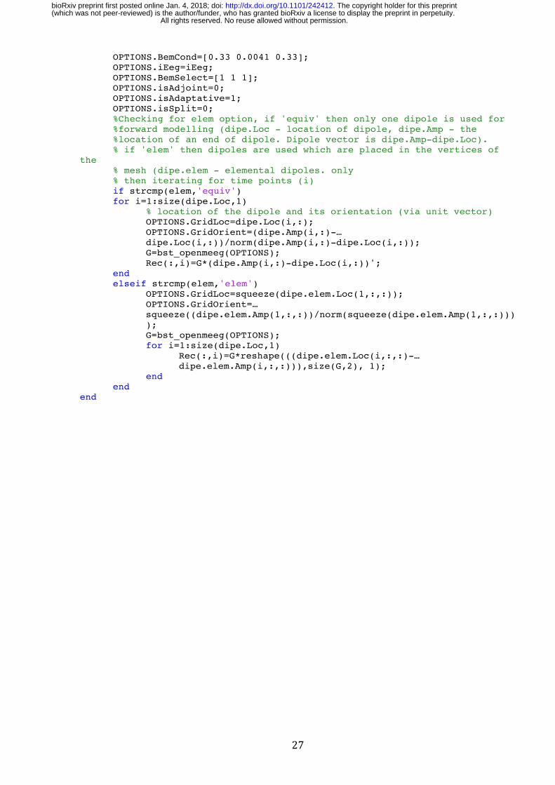
OPTIONS.BemCond=[0.33 0.0041 0.33]; OPTIONS.iEeg=iEeg; OPTIONS.BemSelect=[1 1 1]; OPTIONS.isAdjoint=0; OPTIONS.isAdaptative=1; OPTIONS.isSplit=0; %Checking for elem option, if 'equiv' then only one dipole is used for %forward modelling (dipe.Loc - location of dipole, dipe.Amp - the %location of an end of dipole. Dipole vector is dipe.Amp-dipe.Loc). % if 'elem' then dipoles are used which are placed in the vertices of

the % mesh (dipe.elem - elemental dipoles. only % then iterating for time points (i) if strcmp(elem,'equiv')for i=1:size(dipe.Loc,1)

% location of the dipole and its orientation (via unit vector)OPTIONS.GridLoc=dipe.Loc(i,:); OPTIONS.GridOrient=(dipe.Amp(i,:)-… dipe.Loc(i,:))/norm(dipe.Amp(i,:)-dipe.Loc(i,:)); G=bst_openmeeg(OPTIONS); Rec(:,i)=G*(dipe.Amp(i,:)-dipe.Loc(i,:))';

end elseif strcmp(elem,'elem')

OPTIONS.GridLoc=squeeze(dipe.elem.Loc(1,:,:)); OPTIONS.GridOrient=… squeeze((dipe.elem.Amp(1,:,:))/norm(squeeze(dipe.elem.Amp(1,:,:)))); G=bst_openmeeg(OPTIONS); for i=1:size(dipe.Loc,1)

Rec(:,i)=G*reshape(((dipe.elem.Loc(i,:,:)-… dipe.elem.Amp(i,:,:))),size(G,2), 1);

end end

end



http://dx.doi.org/10.1101/242412

28

Supplementary materials We recommend looping the animation when viewing. Movie 1 Modeling the EEG and equivalent dipole from a radial wave in the visual cortex. Modeled EEG for 100 ms. Electric field distribution on the “scalp” (the occipital-frontal propagation) from a wave in from two symmetric waves in both hemispheres with an epicenter at the vertex 03.008488 of the cortical surface model ICBN152 (the second wave is mirror-wise with respect to the sagittal plane). The equivalent dipole rotates in the sagittal plane at the time indicated by the cursor in EEG window. The current density distribution from radial wave on the unsmoothed and smoothened cortical surface model. Movie 2 Modeling the EEG and equivalent dipole from a radial wave in the visual cortex. Modeled EEG for 100 ms. Electric field distribution on the “scalp” (the counter-clockwise rotation) from a wave in left hemisphere with an epicenter at the vertex 04.18914 of the cortical surface model ICBN152. The equivalent dipole rotates in the axial plane (top view) at the time indicated by the cursor in EEG window. The current density distribution from radial wave on the unsmoothed and smoothened cortical surface model. Movie 3 Modeling the EEG and equivalent dipole from a radial wave in the sensorimotor cortex. Modeled EEG for 100 ms. Electric field distribution on the “scalp” from a wave in left hemisphere with an epicenter at the vertex 19.071133 of the cortical surface model ICBN152. The current density distribution from radial wave on the cortical surface model. The equivalent dipole is precesses within the Rolando fissure. Movies on the site http://braintw.org main->Cortex TW Simulation->Movie-> 170226movCORsim (Cortex TW simulation from 28 epicenters), 170330movEEGsim (EEG TW simulation for 28 epicenters, left and both hemispheres).



http://dx.doi.org/10.1101/242412

The method of modeling the human EEG by calculating radial ... · left hemisphere of the cortical...

Documents

Transcript of The method of modeling the human EEG by calculating radial ... · left hemisphere of the cortical...