TMO Progress Report 42-145 May 15, 2001

The Media Calibration System for CassiniRadio Science: Part II

G. M. Resch,1 J. E. Clark,2 S. J. Keihm,3 G. E. Lanyi,1 C. J. Naudet,1 A. L. Riley,3

H. W. Rosenberger,3 and A. B. Tanner3

A new media calibration system is currently being implemented at DSS 25 thatis intended to calibrate the delay of radio signals due to the neutral atmosphere,both the static dry and static and fluctuating wet components of this delay. In par-ticular, the system will calibrate the fluctuations in path delay due to atmosphericwater vapor that we believe will dominate the error budget for several radio scienceand radio astronomy experiments. The first user of this system will be the Gravita-tional Wave Experiment (GWE) with the Cassini spacecraft. The system consistsof a water vapor radiometer (WVR) of a new design (i.e., the A-series), a microwavetemperature profiler (MTP), and a package of instruments that sense surface mete-orology. In order to demonstrate the performance of the media calibration system,we have installed two of them, one near DSS 13 and one near DSS 15. We operatedthese two radio antennas as an interferometer and compared the estimates of pathdelay provided by the media calibration system to the delay fluctuations seen by theinterferometer. In this article, we describe the instrumentation, observing strategy,data analysis procedures, and weather conditions for 29 interferometer experimentsthat started on August 17, 1999, and ended May 18, 2000. Our goal is to demon-strate that the new media calibration system can meet or exceed an Allan standarddeviation of 3 × 10−15 on time scales of 1,000 to 10,000 s, as required by the CassiniGWE.

I. Introduction

We expect line-of sight delay fluctuations due to water vapor to be a major error source for the Gravi-tational Wave Experiment (GWE) with the Cassini spacecraft that is scheduled to start in December 2001and repeat in 2002 and 2003 during the spacecraft cruise to Saturn. This experiment has been describedby Armstrong et al. [1] and Tinto and Armstrong [2]. In order to calibrate fluctuations in the line-of-sight path delay, two redundant media calibration systems have been designed, constructed, and recentlyinstalled at DSS 25, the primary DSN station for Cassini radio science experiments.

1 Tracking Systems and Applications Section.

2 Allied Signal, Honeywell Technical Services, Inc., Pasadena, California.

3 Microwave and Lidar Technology Section.

The research described in this publication was carried out by the Jet Propulsion Laboratory, California Institute ofTechnology, under a contract with the National Aeronautics and Space Administration.

1

To test this new media calibration system, we have used it in a series of 29 experiments with a radiointerferometer and compared the two very different techniques for sensing path-delay fluctuations. In thisarticle, we describe the instrumentation that was used, the conditions under which the experiments wereperformed, and the data analysis procedures. Preliminary results have been reported by Resch et al. [3]and in Part I of this series of articles [4].

The experiments described here were modeled after the ones described in [5] and [6] using water vaporradiometers (WVRs) of an earlier design. The basic concept of the experiment is illustrated schematicallyin Fig. 1. The radio interferometer is sensitive to any difference in the path of the signal to the two elementscomprising the interferometer. The interferometric observable is the phase-delay difference between thesignals arriving at each antenna. We model and subtract geometric effects so that, in principle, theresidual phase is dominated by effects we cannot model, e.g., fluctuations due to water vapor.

The media calibration system, deployed within 50 m of each antenna, measures the line-of-sight (LOS)delay due to water vapor in the direction of the compact radio source observed with the interferometer.The estimates of LOS delay from each are differenced and then compared with the residual interferometerdelay. If we have modeled all known error sources correctly in the interferometer data, if the mediacalibration system is working as it is designed to do, and if water vapor fluctuations really do dominatethe residual delay variations, then we would expect a high degree of correlation between the residualinterferometer phase and the differenced media calibration system data streams. This is, in fact, whatis observed most of the time. We can then use the differenced WVR data to calibrate and reduce theinterferometer residuals. The measure of our success is whether we can demonstrate that this calibrationholds to an Allan standard deviation (ASD) of 3 × 10−15 over time scales of 1,000 to 10,000 s, therequirement for the Cassini GWE.

DSS 13WVR

CORRELATOR

PATH-DELAY DIFFERENCE

DSS 15

20 km

WATER VAPOR

QUASAR RADIO SOURCE WAVE FRONT

WVR

Fig. 1. A schematic illustration of the comparison experiments between a radiointerferometer and the new media calibration system constructed to support radioscience experiments with the Cassini spacecraft.

2

II. The Radio Interferometer

We used DSS 13 and DSS 15 for all of our experiments, with the two antennas configured as aconnected-element interferometer operating with an approximately 21-km baseline [7]. For a few exper-iments, we added DSS 65 (Spain) or DSS 45 (Australia). All of these 34-m antennas were equippedto receive at the 2.3 GHz (S-band) and 8.45 GHz (X-band) frequencies, and each has a sensitivity ofapproximately 0.25 K/Jy. The total system temperatures at DSS 15, DSS 45, and DSS 65 were typically35 K at S-band and 38 K at X-band, while DSS 13 had 38 K and 40 K at S- and X-band, respectively.Each antenna was also equipped with a Mark IV data acquisition terminal (DAT). A radio source of 1-Jyflux density provides a signal-to-noise ratio (SNR) of approximately 15 for our basic integration time of2 s in the 2-MHz bandwidth of a DAT channel. For most of our experiments, particularly on the shortbaseline, we observed very strong radio sources so that we were rarely SNR limited at time scales longerthan a few seconds.

A fiber-optic cable was used to distribute the primary frequency reference (a hydrogen maser) to thefrequency distribution systems at each antenna. The fiber-optic cable was buried approximately 1.5 mbelow the desert floor and was temperature stable on time scales of days [8]. However, cables betweenthe control room at DSS 13 and the pedestal area under the antenna were partially exposed and thereforesubject to larger temperature variations. The distribution of a single frequency reference to the two radiotelescopes made this a connected-element interferometer (CEI), with better long-term phase stabilitythan a very long baseline interferometer (VLBI).

Another fiber-optic cable was used to send a subset of digital data (14 of 28 channels, each of 4 Mb/sdata rate) from the Mark IV DAT at DSS 15 to the control room at DSS 13, where the data streamsfrom each antenna were cross-correlated using a slightly modified version of the Block II correlator [9],known as the Real Time Block II or RTB2. This provided a real-time confirmation of interferometerperformance and supplied the primary data for our subsequent analysis. In the experiments involvingDSS 45 or DSS 65, we recorded data on the tapes of the Mark IV DAT for later cross-correlation at theBlock II correlator in Pasadena.

III. The Media Calibration System

The media calibration system (MCS) consists of an advanced water vapor radiometer (AWVR) of anew design (i.e., the A-series), a microwave temperature profiler (MTP), and a group of instruments thatsense surface meteorology (SurfMet). To minimize down time during Cassini radio science experiments,the system is redundant, consisting of identical pairs of each instrument. During the interferometryexperiments, one complete instrument suite was located within 50 m of the base of each of the 34-mantennas comprising the CEI.

The AWVR is a room-temperature Dicke radiometer with additive noise injection for gain calibration.The instrument measures atmospheric emissions at three frequencies in the vicinity of the 22-GHz reso-nance line of atmospheric water vapor. The 22.2-GHz channel is the most sensitive to total water-vaporcontent. The 23.8-GHz channel has 20 percent less sensitivity to the total water vapor, but is insensitiveto variations in the vapor height distribution. The 31.4-GHz channel is used primarily to correct for theemission contributions of suspended cloud liquid (when present). Absolute calibration to ∼0.3 K accuracyis achieved by performing a series of tipping curves. The 1-second thermal noise is ∼0.07 K in each of thechannels. Extensive thermal control of the radiometer electronics housing produces long-term stabilityof ∼0.01 K (equivalent to ∼0.03 mm of path delay) on time scales of 10,000 s. The antenna is an offset-fed parabolic reflector that minimizes contaminating radiation from scattering and side lobes and has abeam width of 1 deg (full width at half maximum). The azimuth and elevation steering mechanisms aredesigned to allow complete sky coverage with 0.1-deg pointing accuracy and 0.01-deg pointing knowledgein elevation. A more detailed description of the AWVR is provided by Tanner [10].

3

During the CEI experiments, each AWVR was controlled separately, and the pointing schedules werecoordinated such that each instrument observed the same direction in the sky as the nearby 34-m antennato within 0.1 deg. Brightness temperatures were recorded each 0.4 s together with the azimuth andelevation pointing information. These data comprised the primary observable set for subsequent retrievalsof the wet path-delay time series at either end of the interferometer baseline.

The two microwave temperature profilers (MTPs) were designed and built by Radiometrics Corpora-tion of Boulder, Colorado. These instruments measure sky brightness temperatures at selected frequenciesin the 51- to 59-GHz wing of the molecular oxygen spectral band centered at 60 GHz. Because the at-mosphere is optically thick at these frequencies and oxygen is well mixed in the lower troposphere, thebrightness temperature is a weighted measure of the physical temperature of the air. The variation ofbrightness temperature with elevation angle can be inverted to yield physical temperature versus heightthrough the lower 5 to 7 km of the troposphere.

A brightness temperature calibration accuracy of 0.5 K is achieved with the MTP by using an in-ternal ambient reference and an external liquid nitrogen (∼78 K) target. The liquid nitrogen target isused to calibrate a noise diode (performed every 3 months), which is then used to monitor gain driftsbetween calibrations. The antenna steering mechanism permits all-sky pointing with elevation accuracyof ∼0.1 deg. The effective beam width (full width at half power) varies between 2.3 and 2.5 deg over the51- to 59-GHz channel settings. More detailed description can be found in the reference manual providedby Radiometrics Corporation [11].

During the CEI experiments, the MTPs were operated in a repeating 13-minute elevation scanningmode, measuring sky brightness temperatures at three selected frequencies at elevations of 30, 45, 90,135, and 150 deg in a single azimuth slice. The 13-minute sampling interval is adequate for monitoringtropospheric temperatures that typically vary by less than 0.1 K on 10-minute time scales. A previousstudy by Keihm4 showed that a three-frequency operating mode (53.00, 54.40, and 57.97 GHz), with theabove elevation sampling, is near optimum for temperature profiling in the lower 5 km, where almost allof the water vapor resides.

The group of instruments that measure surface meteorological conditions consists of temperature,pressure, relative humidity, wind speed, and wind direction sensors. All are commercially available prod-ucts. The MET3 weather station, made by Paroscientific of Redmond, Washington, measures ambienttemperature, pressure, and relative humidity. The sensor specifications provided by Paroscientific [12] are0.5 deg C accuracy and 0.01 deg C precision for temperature, 0.1 mb accuracy and 0.001 mb resolution forpressure, and 2 percent accuracy for relative humidity. The MET3 units are returned to the manufacturerannually for recalibration.

The SurfMet instrumentation also includes a sonic anemometer, manufactured by Climatronics ofBohemia, New York, which provides measurements of surface wind speed and direction. The sensorspecifications provided by Climatronics [13] are 1.1 m/h accuracy and 0.22 m/h resolution for windspeed, and 5 deg accuracy and 1 deg resolution for wind speeds in excess of 5 m/h.

For the CEI experiments, 1-minute averages of the temperature, pressure, and relative humiditySurfMet data were used in the estimates of path delay. The wind data were evaluated in a qualita-tive manner in regard to correlations with path-delay fluctuation levels and overall performance of themedia calibration system.

4 S. J. Keihm, Report to Radiometrics on Optimum Channel Selection for a 50-60 GHz MTP, JPL internal document, JetPropulsion Laboratory, Pasadena, California, 1993.

4

IV. The Experiments

Table 1 summarizes the 29 experiments completed in late 1999 and early 2000. We list the scheduledstart date, the actual start time of data acquisition (in Universal time, UT), stop time, and duration, andalso illustrate schematically the distribution of the observations during day/night hours. Our primaryscheduling request was for night hours in order to mimic the conditions under which the GWE would beperformed. The initial observing strategy was to observe a variety of strong sources for approximately26 minutes each. In this way, we were able to track phase fluctuations over a reasonably long period andverify that we could do this at a variety of azimuth and elevation angles. For the experiments in year 2000,we concentrated on longer scans (up to 5 hours) in order to investigate the long-term calibration capabilityof the media calibration system. Total observing time for these experiments amounted to 174.5 hours.

It was not always possible to obtain antenna time during the night, as can be seen in Table 1. Also, we“piggybacked” on several other VLBI experiments between DSS 15 and DSS 65 or between DSS 15 andDSS 45. For these piggyback experiments, we observed a much longer list of radio sources with greatergeometric distribution. The time on each source was approximately 2.5 minutes, and the data were usedto determine the DSS 13–DSS 15 baseline.

Table 2 lists the surface meteorology data taken from the weather station at DSS 13 during eachexperiment and the zenith path delay (ZPD) as estimated by the MCS at each antenna. The data werefiltered to cover only the actual times of observation. The average value of each parameter is listed alongwith the standard deviation about the average. The ZPD variability is a useful indicator of turbulence.

Table 3 lists the surface meteorology data from the MCS located at DSS 15 and from the weatherinstruments at Signal Processing Center (SPC) 10. The separation of these instrument packages is onthe order of 300 m. Note the SurfMet instruments were installed as they became available but after ourexperiments started in late 1999. We were not able to install wind speed and direction sensors at theDSS-15 location, so those columns are blank in Table 3.

We rely primarily on data from the SurfMet package of sensors in our data analysis, but when it wasnot available we use the data from the weather stations at DSS 13 and SPC 10. Both were within a fewhundred meters of the SurfMet instruments, which were closer to the antennas at DSS 13 and DSS 15.Figures 2 and 3 show scatter plots of the overlapping surface meteorological data from the DSS-13 weatherstation (the x-axis) and the SurfMet package (the y-axis). In Fig. 2, we plot the pressure, temperature,and relative humidity. Each figure also provides the analytical expression for the regression line of thedata. In general, the correlation is very good and, except for the pressure, the offsets are reasonable. InFig. 3, we plot the wind direction and wind speed. Here, a 180-deg convention between the sensors isapparent. The DSS-13 sensor reports the direction the wind is coming from while the SurfMet packagereports the direction the wind is heading. Note that the prevailing wind at DSS 13 is from the westby southwest. Our MCS is located on a line to the southeast of the 34-m antenna, which means thatsurface winds blow almost perpendicularly to the line between the MCS and the antenna it is calibrating.This geometry, together with the prevailing winds, tends to suppresses short-term correlation betweenthe MCS and CEI data.

In Fig. 4, we show the scatter plots between the SurfMet data (x-axis) and the weather station dataat SPC 10. The regression line formula is provided for each plot. Again, the correlation is good and thebias terms small. We conclude that we can use either the SurfMet data or the weather-station data atGoldstone (corrected by the regression lines) and maintain consistency in our data analysis.

Figures 5 and 6 show the time history of the ZPD (top panel of each figure) for days of year (DOYs) 229and 240 from 1999. Similar plots are generated for each experiment. The top panel shows the ZPD versustime, and the bottom panel of each figure plots the site-differenced ZPD along with the best linear fit. Alinear (in time) change in the zenith path delay would show up later in the analysis of the CEI data asan apparent clock drift rate. In acquiring these data, the AWVRs were pointed along the LOS and the data

5

Dur

atio

n,h

Stop

,U

TSt

art,

UT

Uni

vers

al T

ime,

hD

OY

Dat

e

Tab

le 1

. S

um

mar

y o

f ex

per

imen

t d

ates

, tim

es, d

ura

tio

n, a

nd

dis

trib

uti

on

du

rin

g t

he

day

. (S

had

ed a

rea

den

ote

s n

igh

t.)

6

Tab

le 2

. S

um

mar

y o

f su

rfac

e w

eath

er c

on

dit

ion

s (f

rom

th

e D

SS

-13

wea

ther

sta

tio

n)

du

rin

g t

he

exp

erim

ents

an

d t

he

ZP

D a

s es

tim

ated

by

the

MC

S a

tD

SS

13

(A1)

an

d D

SS

15

(A2)

. (C

olu

mn

s la

bel

ed σ

are

th

e st

and

ard

dev

iati

on

s o

f th

e in

div

idu

al v

alu

es in

th

e p

rece

din

g c

olu

mn

du

rin

g a

n e

xper

imen

t.)

DO

YD

ate

Pre

ssur

e,m

bσ

Tem

pera

ture

,de

g C

Rel

ativ

eH

umid

ity,

perc

ent

Win

dD

irect

ion,

deg

Win

dS

peed

,m

ph

Ave

rage

ZP

D-A

1,cm

Ave

rage

ZP

D-A

2,cm

σσ

σσ

σσ

7

Pres

sure

,M

b

SurfM

et S

ubsy

stem

at D

SS 1

5

DO

YD

ate

Wea

ther

Sta

tion

at S

PC 1

0

σTe

mpe

ratu

re,

deg

Cσ

σ

Rela

tive

hum

idity

,pe

rcen

tPr

essu

re,

Mb

σTe

mpe

ratu

re,

deg

Cσ

σ

Rela

tive

hum

idity

,pe

rcen

t

Tab

le 3

. Su

mm

ary

of

the

surf

ace

met

eoro

log

ical

dat

a fr

om

th

e M

CS

at

DS

S 1

5 th

at b

ecam

e av

aila

ble

sta

rtin

g in

Jan

uar

y 20

00 a

nd

the

wea

ther

inst

rum

ents

loca

ted

at

SP

C 1

0. (

σ d

eno

tes

the

stan

dar

d d

evia

tio

n o

f th

e m

easu

rem

ents

du

rin

g t

he

exp

erim

ent.

)

8

scaled to zenith as described below. These plots offer an illustration of the dynamics of the atmosphereover 21-km baselines and are also useful for data-editing purposes.

V. Data Analysis Procedures

A. Estimating the Wet Path Delay

During the interferometry experiments, each AWVR measured the brightness temperature along itsline of sight (co-pointed with the nearby DSN antenna) at 0.4-s intervals and produced a time-taggedseries of data that included the AWVR azimuth and elevation angles. These brightness-temperature datawere then averaged over 6-s intervals, sufficient to reduce thermal noise with no significant loss of path-delay fluctuation information. The MTP observables (13-min sampling) and SurfMet observables (1-minsampling) were then interpolated to the 6-s AWVR time tags. Thus, the complete set of time-tagged inputfor algorithms to estimate path delay consisted of 16 observables: 3 AWVR LOS brightness temperatures,1 AWVR elevation angle, 9 MTP brightness temperatures (3 channels times 3 fixed elevation angles), and

f (x ) = 8.970180 × 10−1 × x + −2.242333 × 100

R 2 = 2.901957 × 10−1

50 60 70 80 90

DSS-13 RELATIVE HUMIDITY, percent

403020100

90

80

50

40

0

SU

RF

ME

T R

ELA

TIV

E H

UM

IDIT

Y, p

erce

nt

70

60

30

20

10 (c)

f (x ) = 1.007614 × 100 × x + −2.586816 × 100

R 2 = 9.798025 × 10-1

30

DSS-13 TEMPERATURE, deg C

252015100

30

25

20

15

0

SU

RF

ME

T T

EM

PE

RA

TU

RE

, deg

C

10

5

5

(b)

f (x ) = 9.932867 × 10−1 × x + 5.012247 × 100

R 2 = 9.992496 × 10−1

905

900

895

890

885885 890 895 900 905

DSS-13 PRESSURE, mb

SU

RF

ME

T P

RE

SS

UR

E, m

b

(a)

Fig. 2. Scatter plots of surface meteorological data from the DSS-13 weather station (x-axis) versus the SurfMetinstruments in the MCS (y-axis): (a) pressure, (b) temperature, and (c) relative humidity. Also shown is theexpression for the regression line of each plot.

9

f (x ) = 7.385404 × 10−1 × x + 7.105110 × 10−1

R 2 = 9.716918 × 10−1

25 30

DSS-13 WIND SPEED, km/s

20151050

30

25

20

0

SU

RF

ME

T W

IND

SP

EE

D, k

m/s

15

10

5

(b)

f (x ) = 3.041362 × 10−1 × x + 6.868367 × 101

R 2 = 1.126621 × 10−1

150

DSS-13 WIND DIRECTION, deg

1000

150

0

SU

RF

ME

T W

IND

DIR

EC

TIO

N, d

eg

100

50

50

(a)

Fig. 3. Scatter plots of the (a) wind direction and (b) wind speed from the DSS-13 weather station (x-axis) andthe SurfMet instruments (y-axis). Also shown are the regression line and correlation of each plot.

3 SurfMet measurements (temperature, pressure, and relative humidity). These time series were usedwith both a statistical retrieval algorithm [14], and, for some of the cloud-free experiments, a Bayesianretrieval algorithm [15] to estimate the line-of-sight delay.

The statistical algorithm retrieves the ZPD from a linear combination of all the observables, except-ing the AWVR pointing elevation angle. The ZPD can then be converted to the elevation angle of thenearby DSN antenna (at the AWVR time tag) using an appropriate mapping function. The AWVRelevation-angle value is used first to convert the LOS brightness temperatures to zenith-equivalent values,as described below. This conversion is required to avoid the necessity of computing retrieval coefficientsthat depend on the time-varying AWVR elevation. By the conversion to zenith, a single set of retrievalcoefficients can be applied to the entire track of an experiment. The retrieval coefficients are generatedby regression fits using Desert Rock, Nevada, radiosonde-based archives of the SurfMet values, computedAWVR (zenith) and MTP (90-, 45-, and 30-deg elevation) brightness temperatures, and computed ZPD.The Desert Rock database was selected as our best match for the altitude and climatology of Goldstone.By stratifying the database according to clear-only or all-weather conditions, separate sets of retrievalcoefficients were generated for clear and cloudy conditions. A simple statistical retrieval for cloud liq-uid burden, using only the AWVR brightness temperature measurements, Tb(θ), was implemented todetermine the appropriate set of retrieval coefficients for a given experiment.

In order to implement the statistical algorithm, the brightness temperatures were first converted tozenith-equivalent values by using an approximation relating the elevation dependence of LOS brightnesstemperatures to zenith opacity and air mass:

Tb(θ) = TM − (TM − TC)× exp(−m× τ0) (1)

where τ0 is the zenith opacity, m(θ) is the air mass at elevation θ, TC is the cosmic background tempera-ture, and TM is the mean radiating temperature of the atmospheric emissions. One can estimate TM fromthe surface-temperature measurement (using regressions from radiosonde calculations) to ∼3 K rms accu-racy. Then, with the assumption of a plane-parallel atmosphere, m(θ) = 1/ sin(θ), the zenith-equivalentbrightness temperature, Tbz, can be derived from the LOS Tb measurements as

10

f (x ) = 9.875621 × 10−1 × x + 1.135728 × 101

R 2 = 9.994474 × 10−1

909

903

901

899

897897 899 901 903 909

SURFMET PRESSURE, mb

SP

C 1

0 P

RE

SS

UR

E, m

b

(a)

905 907

905

907

f (x ) = 8.986822 × 10−1 × x + 2.904031 × 101

R 2 = 9.814068 × 10−1

300

SURFMET TEMPERATURE, K

295290285275

300

295

290

275

SP

C 1

0 T

EM

PE

RA

TU

RE

, K

285

280

280

(b)

f (x ) = 8.707388 × 10−1 × x + 2.058064 × 100

R 2 = 9.965497 × 10−1

50 60 70 80

SURFMET RELATIVE HUMIDITY, percent

403020100

80

50

40

0

SP

C 1

0 R

ELA

TIV

E H

UM

IDIT

Y, p

erce

nt70

60

30

20

10(c)

Fig. 4. Scatter plots of surface meteorological data from the SurfMet instruments located at DSS 15 (x-axis)versus the weather data from SPC 10 (y-axis): (a) pressure, (b) temperature, and (c) relative humidity. Alsoshown is the expression for the regression line of each plot.

Tbz = Tb(θ = 90o) = TM − (TM − TC)×[TM − Tb(θ)TM − TC

]sin(θ)

(2)

The sensitivity of the computed Tbz in Eq. (2) to errors in TM is small and increases with opacity. Fora wet zenith delay of 10 cm, a 3-K error in TM will cause only a 0.05-K error in the Tbz value obtainedfrom a 20-deg elevation LOS measurement. Simulations have confirmed that the errors in zenith delayretrieved in this way are not significantly worse than the errors in zenith delay retrieved from direct Tbzmeasurements [17].

The Bayesian algorithm estimates the path delay by a direct inversion process that finds the “mostprobable” atmospheric state vector (surface pressure plus discrete height temperature and water-vapordensity profiles) that is consistent with both the 16 measured observables and a priori statistics of the

11

ZE

NIT

H P

AT

H D

ELA

Y, c

mZ

PD

DIF

FE

RE

NC

E, c

m

8

A1 ZPD

A2 ZPD9

10

11

12(a)

−1.5

−1.0

−0.5

0.0

0.5

6 7 8 9 10 11 12

UT, h

A2−A1

1.0

Fig. 5. The experiment on August 17, 1999 (DOY 229-1999): (a) ZPD versus time and (b) site-differenced ZPD versus time. (The AWVR denoted as A1 was located at DSS 13, and A2 was locatedat DSS 15.)

(b)

ZP

D D

IFF

ER

EN

CE

, cm

ZE

NIT

H P

AT

H D

ELA

Y, c

m

0.8

1.01.2

1.4

1.6

16.0

UT, h

A2−A1

1.8

Fig. 6. The experiment on August 28, 1999 (DOY 240-1999): (a) ZPD versus time and (b) site-differenced ZPD versus time. (The AWVR denoted as A1 was located at DSS 13, and A2 was locatedat DSS 15.)

(b)

16.5 17.0 17.5 18.0 18.5 19.0 19.5 20.0 20.5

0.60.40.20.0

A1 ZPD

A2 ZPD

4.5(a)

4.0

3.5

3.0

2.5

2.0

12

atmosphere (derived from the Desert Rock radiosonde archive). For a given set of observables, thecandidate state vector solution “probability” depends both on its conformity to the a prior statisticsand a minimization of residuals between the measured observables and theoretical observables computedfrom the candidate state vector using a radiative transfer model. Probabilities are computed assumingGaussian statistics for both the components of the atmospheric state vector and the observable errors.An iterative process is implemented to find the most probable state vector, from which the zenith wetdelay estimate is computed directly. For more details and comparisons of the performance of the Bayesianand statistical algorithms, see [14] and [15].

We have noted that the Bayesian algorithm is only implemented for clear conditions. Inclusion ofclouds, with variable base height and thickness, and the strong temperature dependency of the absorp-tion due to suspended water droplets lead to instabilities in the solution iteration process that make theBayesian algorithm impractical for cloudy cases. As described in a previous study [16], the major advan-tages of the Bayesian algorithm are seen for clear conditions when MTP information is available. For theshort-baseline interferometry experiments at Goldstone, the tropospheric temperature profiles will nor-mally be similar enough at each end of the 21-km baseline that site-differenced path-delay retrievals willremove algorithm errors related to temperature profile effects, thereby mitigating the expected Bayesian-versus-statistical algorithm improvements expected for a single site. Thus, we have generated the morecomplex Bayesian algorithm solutions for only a small subset of the clear experiments and have found nosignificant improvement relative to the statistical algorithm.

In the development and implementation of both the statistical and Bayesian path-delay retrievalalgorithms, a plane-parallel atmosphere is assumed; i.e., temperature, pressure, and humidity are assumedconstant across horizontal layers. The effect of Earth curvature is to shorten the path length at the lowerelevation angles, reducing both the LOS air mass and brightness temperatures by small amounts. Itis straightforward to account for the curvature effect on the LOS brightness temperatures by adding asmall Tb increment dependent on opacity and elevation angle.5 However, this correction has not yet beenimplemented in the preliminary processing of the tropospheric calibration data for the CEI experiments.Because the final data product is the site-differenced delay over a short baseline (with nearly equal AWVRelevation angles), the small errors due to neglect of the Earth-curvature effect are expected to essentiallycancel.

After the data from each set of MCS instruments were processed to produce ZPD time series at theDSS-13 and DSS-15 sites, the results were differenced to provide an estimate of the differential phasedelay between the two stations that could then be compared with the CEI residual phase delay. Thecomparisons were made after a linear trend was removed from the site-differenced time series to provideconsistency with the clock-error correction inherent to the CEI processing.

Note that the above description of media calibration processing does not include dry delay effects. Fora given site, the hydrostatic (dry) zenith delay depends only on surface pressure, PS [16]. At Goldstone,the relationship is

ZPDD = 0.2279× PS (3)

where PS is the total surface pressure in millibars (mb) and ZPD is in units of cm. For the CEI experimentsprior to January 15, 2000, we did not have a SurfMet station operating at DSS 15 and therefore assumedthat the DSS-13 SurfMet measurements could be applied at both sites. This assumption eliminatedconsideration of a site-difference component due to the dry delay. Since January 15, 2000, SurfMetstations at both the DSS-13 and DSS-15 ends of the CEI baseline have been operative, and we have

5 S. J. Keihm, “Elevation Angle and Earth Curvature Issues Relevant to the Zenith Wet Path Delay Retrieval Algorithms,”JPL internal document, Jet Propulsion Laboratory, Pasadena, California, December 7, 2000.

13

added the small site-differenced dry delay components to the media calibration system wet delay results.Preliminary results indicate that the site-differenced dry component is rarely significant relative to thewet delay from the media calibration system in comparisons with CEI phase delay results.

The ZPD data from each MCS constitutes a time series of data, consisting of brightness-temperaturefluctuations from atmospheric water-vapor and instrumental noise. After the brightness temperatures areconverted to delay, we can write the time series of zenith path delay for each MCS as

SW1 = Satm1 +NW1

SW2 = Satm2 +NW1

(4)

These data are then differenced to provide an estimate of the differential phase delay between the twostations with the result expressed as

∆SW = ∆Satm +NW1 +NW1 (5)

where NW1 and NW2 are the noise contributions from the respective MCS instruments and ∆Satm is thewet component of the differential atmospheric delay.

B. Interferometric Path Delay

The experiment is illustrated schematically in Fig. 1. The observable is interferometer phase delay,which is inherently a differential data type sensitive to the difference in path length between the elementsof the interferometer. The difference in time of arrival, or delay τ , at the two antennas of a CEI is simply

τ =~B • sc

+ τatm + τinst (6)

where ~B is the vector baseline between the two antennas, s is the unit vector in the direction of the sourcebeing observed, c is the speed of light, τatm is the delay due to the difference in atmospheric path, andτinst is the difference in instrumental delay.

As a radio source is tracked by the interferometer, the delay changes continuously due to Earth ro-tation. The cross-correlation process of the CEI data uses a priori estimates of the baseline and sourceposition (and several other parameters as well) in order to produce residual path delay and delay rate [9].The interferometer can be visualized as having an interference pattern in the plane of the sky with thealternate regions of in-phase and out-of-phase regions called fringes. As the radio source appears to movethrough these fringes, the output of the correlator is a sinusoidal variation. The correlator effectivelyslows this variation by modeling the changes in geometry, i.e., it calculates and subtracts the dot-productterm in the equation above. In principle, we are then left with (1) the differential atmospheric delay,(2) any differences in the instrumental delay, and (3) any errors due to imperfect modeling in the corre-lator.

The output of the correlator is then transferred to our fringe-fitting software [17], which solves for thebest estimate of the phase delay and delay rate for each scan. It also removes a term in the phase-delayestimate that is linear in time. This results in an estimate of phase delay that is zero mean over the scanand removes the constant term in the differential instrumental delay as well as any terms that are linearin time, e.g., a clock-rate offset. Next, we correct for any known error that was made in the a priori datarequired to run the correlator and then map the CEI data to zenith using the same mapping function as

14

was used with the MCS data. Note that small differences between the pointing of the AWVR and nearby34-m antenna are reduced by this process.

The resulting time series of CEI data, which we will denote as SI , is then approximately the differencein atmospheric delay to the two antennas plus the noise of the interferometer, or

SI = ∆Satm +NI (7)

A graphical example of the time series represented by Eqs. (5) and (7) is shown in Fig. 7. Here we plotdata from one of our first experiments, DOY 240, August 28, 1999. During this experiment, we observednine radio sources, each for a period of 26 minutes, at a variety of elevation angles ranging from 15 degup to 72 deg. This experiment started a little after 9 a.m. (PDT) and lasted for 3 hours. For reference,the total zenith path delays from the two MCS instruments and their difference are shown in the twopanels of Fig. 6. The barometer was steady, the surface temperatures were rising at both ends of theinterferometer, and the surface winds were light (i.e., 2 m/s) and from the southwesterly direction. Thiswas a relatively dry day with moderate fluctuations at our Goldstone complex.

Figure 7 shows the residual CEI phase delay plotted on the same scale as the differenced MCS data,after a linear trend had been removed from each time series. The high degree of correlation in thefluctuations is obvious. If the interferometer and MCS instruments sense the exact same atmosphericfluctuation, ∆Satm, then we can subtract the differential estimate of the LOS path delay provided by theMCS instruments from the interferometer data and we are left with

RC = SI −∆SW

= NI − (NW1 +NW2) (8)

where RC = RC(t) is the corrected time series. Note that the “noise” terms for both the interferometerand the AWVR contain both statistical as well as systematic error. The time series of Eq. (8) should bezero mean and have a variance of

RE

SID

UA

L Z

PD

, cm

−0.2

0.0

0.2

0.4

16.0

UT, h

RESIDUAL CEI

0.6

Fig. 7. The residual time delay from the interferometer and the differenced MCS data(scaled to zenith) after a linear trend is removed from each.

16.5 17.0 17.5 18.0 18.5 19.0 19.5 20.0 20.5

−0.4

−0.6

RESIDUAL AWVR

15

∆R2C = ∆N2

I + 2×∆N2W (9)

where we have assumed that the two MCS instruments have the same noise variance. Figure 8 shows theresult of subtracting Eq. (5) from Eq. (7), i.e., calibrating the CEI residuals with the differenced MCSdata. On average, the rms fluctuations are reduced by a factor of 2.7 for these 8 observations. Anotherway to look at these data is illustrated in Fig. 9, where we plot the histograms of the residuals for the threedata types. The 2-s points of each time series for all 8 observations were binned and counted to producethese plots. We see that the broad, slightly asymmetric distributions of the CEI and MCS data, whencombined, produce a much narrower and more Gaussian-looking distribution of the calibrated residuals.

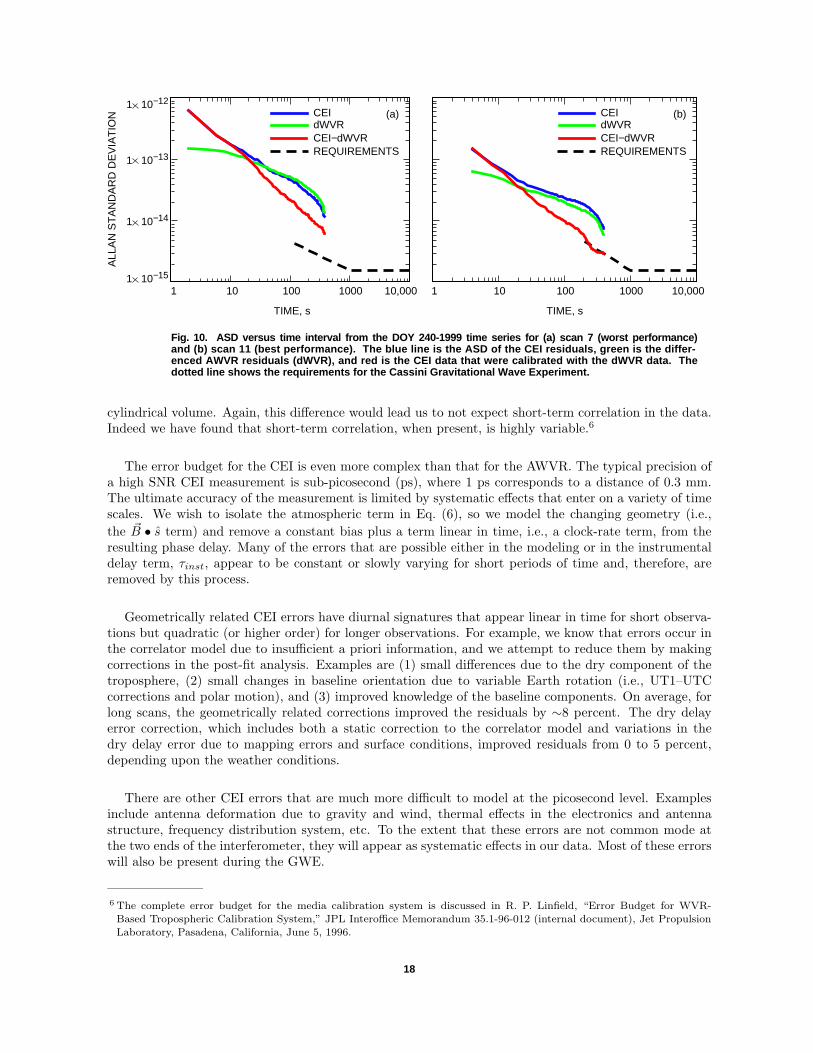
Finally, we calculate the Allan standard deviation (ASD) [18] of the interferometer phase residualsbefore correction, using the time series given by Eq. (7), the ASD of the differenced MCS data usingEq. (5), and the corrected CEI data using the time series of Eq. (8) to assess the MCS performance.Figure 10 illustrates these ASD results for two scans taken during DOY 240, 1999, and represent theworst (scan 7) and best (scan 11) performance that day. The dotted line in each plot represents therequirement specification for the Cassini GWE.

CA

LIB

RA

TE

D R

ES

IDU

AL

ZP

D, c

m

−0.2

0.0

0.2

0.4

16.0

UT, h

0.6

Fig. 8. The residual interferometer phase delay from after the differenced MCS wassubtracted, i.e., the calibrated CEI data.

16.5 17.0 17.5 18.0 18.5 19.0 19.5 20.0 20.5

−0.4

−0.6

RESIDUAL DIFFERENCE

VI. Discussion

We have designed these experiments to mimic, in some respects, the Gravitational Wave Experimentthat will be performed with the Cassini spacecraft during its cruise to Saturn. The GWE will involvea two-way link that will have a round-trip light-time of a few hours, whereas the experiments describedhere involve two receive-only antennas separated by approximately 20 km. In a sense, one can think ofthe experiments we describe as a spatial interferometer while the GWE is a temporal interferometer. TheCEI experiments and the GWE have many common elements in their respective error budgets.

In the discussion in Section 5 regarding the comparison of the time series, we have neglected mentionof systematic errors. In the case of the MCS, there are other considerations, such as the size of the AWVRsensing beam and the offset of this beam relative to that of the 34-m antenna, that will cause errors thatdo not appear as white noise. While we can calculate the qualitative impact of these effects [19], theiractual contribution is often dependent on meteorological conditions during an experiment.

16

NU

MB

ER

PE

R IN

TE

RV

AL

NU

MB

ER

PE

R IN

TE

RV

AL

1800

(b)1600

1400

1200

1000

800

600

400

200

0

1800

(a)1600

1400

1200

1000

800

600

400

2000

0.45

0

INTERVAL OF RESIDUAL DELAY, cm

1800

Fig. 9. Histograms of residual delays from DOY 240-1999: (a) CEI residuals,(b) AWVR residuals, and (c) calibrated CEI data.

(c)

−0.4

25

−0.3

75

−0.3

25

−0.2

75

−0.2

25

−0.1

75

−0.1

25

−0.0

75

−0.0

25

0.02

5

0.07

5

0.12

5

0.17

5

0.22

5

0.27

5

0.32

5

0.37

5

0.42

5

0.45

0

1600

1400

1200

1000

800

600

400

200

0

NU

MB

ER

PE

R IN

TE

RV

AL

< − < −

RMS = 0.114 cm

RMS = 0.107 cm

RMS = 0.041 cm

For example, the AWVRs are located approximately 50 m from the base of the associated 34-m ele-ment of the interferometer. A “blob” of water vapor being convected horizontally at a speed of 10 km/halong the line between the AWVR and 34-m antenna will take about 18 s to make the trip. This implieswe should not expect the time series discussed above to correlate very well on short time scales (e.g.,<100 s), and the correlation time scale will depend on wind speed as well as where the antennas arepointing. In fact, it may depend on the wind speed at altitude rather than at the surface—a quantity wedo not sense. Also, the sensing volume of the AWVR beam is approximately a cone with an opening angleof 1 deg whereas, to the 34-m antenna, the atmosphere is a near-field phenomena, and the antenna senses a

17

CEIdWVRCEI−dWVRREQUIREMENTS

1 10 100 1000 10,000

TIME, s

1 10−15

1 10−14

ALL

AN

ST

AN

DA

RD

DE

VIA

TIO

N

1 10−13

1 10−12

1 10 100 1000 10,000

TIME, s

CEIdWVRCEI−dWVRREQUIREMENTS

(a) (b)

Fig. 10. ASD versus time interval from the DOY 240-1999 time series for (a) scan 7 (worst performance)and (b) scan 11 (best performance). The blue line is the ASD of the CEI residuals, green is the differ-enced AWVR residuals (dWVR), and red is the CEI data that were calibrated with the dWVR data. Thedotted line shows the requirements for the Cassini Gravitational Wave Experiment.

cylindrical volume. Again, this difference would lead us to not expect short-term correlation in the data.Indeed we have found that short-term correlation, when present, is highly variable.6

The error budget for the CEI is even more complex than that for the AWVR. The typical precision ofa high SNR CEI measurement is sub-picosecond (ps), where 1 ps corresponds to a distance of 0.3 mm.The ultimate accuracy of the measurement is limited by systematic effects that enter on a variety of timescales. We wish to isolate the atmospheric term in Eq. (6), so we model the changing geometry (i.e.,the ~B • s term) and remove a constant bias plus a term linear in time, i.e., a clock-rate term, from theresulting phase delay. Many of the errors that are possible either in the modeling or in the instrumentaldelay term, τinst, appear to be constant or slowly varying for short periods of time and, therefore, areremoved by this process.

Geometrically related CEI errors have diurnal signatures that appear linear in time for short observa-tions but quadratic (or higher order) for longer observations. For example, we know that errors occur inthe correlator model due to insufficient a priori information, and we attempt to reduce them by makingcorrections in the post-fit analysis. Examples are (1) small differences due to the dry component of thetroposphere, (2) small changes in baseline orientation due to variable Earth rotation (i.e., UT1–UTCcorrections and polar motion), and (3) improved knowledge of the baseline components. On average, forlong scans, the geometrically related corrections improved the residuals by ∼8 percent. The dry delayerror correction, which includes both a static correction to the correlator model and variations in thedry delay error due to mapping errors and surface conditions, improved residuals from 0 to 5 percent,depending upon the weather conditions.

There are other CEI errors that are much more difficult to model at the picosecond level. Examplesinclude antenna deformation due to gravity and wind, thermal effects in the electronics and antennastructure, frequency distribution system, etc. To the extent that these errors are not common mode atthe two ends of the interferometer, they will appear as systematic effects in our data. Most of these errorswill also be present during the GWE.

6 The complete error budget for the media calibration system is discussed in R. P. Linfield, “Error Budget for WVR-Based Tropospheric Calibration System,” JPL Interoffice Memorandum 35.1-96-012 (internal document), Jet PropulsionLaboratory, Pasadena, California, June 5, 1996.

18

VII. Summary

The data described in this article are currently being analyzed. Preliminary analysis suggests the newmedia calibration system does meet Cassini requirements some of the time. At this juncture, the limitingfactor in the comparison between CEI and the MCS is not clear, but we strongly suspect systematicerrors in the CEI data.

In late 2000 there was a significant upgrade to the frequency distribution system between SPC 10and DSS 13 that we expect will improve CEI long-term performance, and additional experiments wereconducted between December 2000 and February 2001. These experiments and results of the analysis ofexperiments described here will be described in a future issue of this publication.

Acknowledgments

We are very grateful to Lyle Skjerve, Leroy Tanida, Charles Snedeker, the staffat DSS 13, and the Operations crews at the Goldstone Signal Processing Center forthe invaluable assistance they provided during these experiments.

References

[1] J. W. Armstrong, B. Bertotti, F. B. Estabrook, L. Iess, and H. D. Wahlquist,“The Galileo/Mars Observer/Ulysses Coincidence Experiment,” Proc. of theSecond Edoardo Amaldi Conf. on Gravitational Waves, edited by E. Coccia,G. Pizzella, and G. Veneziano, Edoardo Amaldi Foundation Series, vol. 4, WorldScientific, Geneva, Switzerland, July 1–4, 1997, pp. 159–167, 1998.

[2] M. Tinto and J. W. Armstrong “Spacecraft Doppler Tracking as a Narrow-Band Detector of Gravitational Radiation,” Phys. Rev. D, vol. 58, 042002,pp. 042002-1–042002-8, 1998.

[3] G. M. Resch, C. Jacobs, S. Keihm, G. Lanyi, C. Naudet, A. Riley, H. Rosenberger,and A. Tanner, “Calibration of Atmospherically Induced Delay Fluctuations dueto Water Vapor,” International VLBI Service for Geodesy and Astrometry 2000General Meeting Proceedings, edited by N. R. Vandenberg and K. D. Baver,NASA/CP-2000-209893, Kotzting, Germany, pp. 274–279, 2000.

[4] C. Naudet, C. Jacobs, S. Keihm, G. Lanyi, R. Linfield, G. Resch, L. Riley,H. Rosenberger, and A. Tanner, “The Media Calibration System for CassiniRadio Science: Part I,” The Telecommunications and Mission OperationsProgress Report 42-143, July–September 2000, Jet Propulsion Laboratory, Pasa-dena, California, pp. 1–8, November 15, 2000.http://tmo.jpl.nasa.gov/tmo/progress report/42-143/143I.pdf

[5] G. M. Resch, D. E. Hogg, and P. J. Napier, “Radiometric Correction of Atmo-spheric Path Length Fluctuations in Interferometric Experiments,” Radio Sci.,vol. 19, pp. 411–422, January 1984.

19

[6] L. P. Teitelbaum, S. J. Keihm, R. P. Linfield, M. J. Mahoney, and G. M. Resch,“A Demonstration of Precise Calibration of Tropospheric Delay Fluctuationswith Water Vapor Radiometers,” Geophys. Res. Lett., vol. 23, no. 25, pp. 3719–3722, December 1996.

[7] C. Edwards, Jr., D. Rogstad, D. Fort, L. White, and B. Iijima, “The Gold-stone Real-Time Connected Element Interferometer,” The Telecommunicationsand Data Acquisition Progress Report 42-110, April–June 1992, Jet PropulsionLaboratory, Pasadena, California, pp. 52–62, August 15, 1992.http://tmo.jpl.nasa.gov/tmo/progress report/42-110/110D.PDF

[8] G. Lutes and A. Kirk, “Reference Frequency Transmission Over Optical Fiber,”The Telecommunications and Data Acquisition Progress Report 42-87, July–September 1986, Jet Propulsion Laboratory, Pasadena, California, pp. 1–9,November 15, 1986.http://tmo.jpl.nasa.gov/tmo/progress report/42-87/87A.PDF

[9] J. B. Thomas, Interferometric Theory for the Block II Processor, JPL Publication87-29, Jet Propulsion Laboratory, Pasadena, California, October 15, 1987.

[10] A. B. Tanner, “Development of a High-Stability Water Vapor Radiometer,”Radio Sci., vol. 33, pp. 449–462, March 1998.

[11] TP-2500 Temperature Profiling Radiometer, User’s Manual, Radiometrics Cor-poration, Boulder, Colorado, November 1998.

[12] Met3 Meteorological Measurement System, Document T8360-001, Rev. D, Paro-scientific, Inc., Redmond, Washington, 1999.

[13] Sonic Anenometer, Manual for p/n M102263, Climatronics Corp., Bohemia, NewYork, 1999.

[14] G. M. Resch, M. C. Chavez, N. I. Yamane, K. M. Barbier, and R. C. Chan-dlee, Water Vapor Radiometry Research and Development Phase Final Report,JPL Publication 85-14, Jet Propulsion Laboratory, Pasadena, California, April1, 1985.

[15] S. J. Keihm and S. Marsh, “New Model-Based Bayesian Inversion Algorithm forthe Retrieval of Wet Tropospheric Path Delay from Radiometric Measurements,”Radio Sci., vol. 33, no. 2, pp. 411–419, March 1998.

[16] J. Saastamoinnen, “Atmospheric Correction for the Troposphere and Strato-sphere in Radio Ranging of Satellites,” in The Use of Artificial Satellitesfor Geodesy, Geophysics Monograph, series 15, American Geophysical Union,pp. 247–251, 1972.

[17] S. Lowe, Theory of Post-Block II VLBI Observable Extraction, JPL Publication92-7, Jet Propulsion Laboratory, Pasadena, California, July 15, 1992.

[18] D. W. Allan, “Statistics of Atomic Frequency Standards,” Proc. IEEE, vol. 54,no. 2, pp. 221–230, February 1966.

[19] R. P. Linfield and J. Z. Wilcox, “Radio Metric Errors Due to Mismatch andOffset Between a DSN Antenna Beam and the Beam of a Tropospheric Calibra-tion Instrument,” The Telecommunications and Data Acquisition Progress Report42-114, April–June 1993, Jet Propulsion Laboratory, Pasadena, California,pp. 1–13, August 15, 1993.http://tmo.jpl.nasa.gov/tmo/progress report/42-114/114A.pdf

20