1

The Measurement of Business Capital, Income and Performance Tutorial presented at the University Autonoma of Barcelona, Spain, September 21-22, 2005; revised December, 2005. W. Erwin Diewert, Department of Economics, University of British Columbia, Vancouver, B.C., Canada, V6N 1Z1 Email: diewert@econ.ubc.ca VIII. The Measurement of Performance: Productivity versus the Real Rate of Return 1. Introduction 2. Productivity Measurement in the Case of One Input and One Output 3. The Determinants of Economic Growth: Primary Input Growth and Other Factors 4. The Determinants of Economic Growth: Productivity Growth 5. Increasing Returns to Scale 6. Other Factors that Might Explain Growth 7. A Summary of the Factors Explaining Productivity Growth 8. The Role of Government in Facilitating Growth. 9. The Index Number Approach to the Measurement of Productivity 10. The Estimation of Technical Progress and Returns to Scale 11. Can the Use of Instrumental Variables Lead to Better Estimates of Returns to Scale? 1. Introduction There are three main methods that could be used to measure the performance of one market oriented business unit or production unit1 against the performance of other units:

• Compare the real rate of return that the production unit earns over a time period with the corresponding real rates of return that peer group production units earn over similar periods of time;

• Compare the Total Factor Productivity of the business unit with its productivity in a prior period or with a comparable group of production units; or

• Benchmark the performance of the production unit with that of its peers. We will look at the benchmarking methodology in the following chapter so in the present chapter, we will concentrate on the first two methods.

1 A production unit could be an establishment, a firm, an industry or an entire economy.

2

The real rate of return methodological approach works as follows:

• Calculate the value of outputs produced by the unit over a standard period of time (say period 0) less the value of all inputs used, excluding the capital inputs. This is essentially the Gross Operating Surplus of the production unit (GOS0).

• Calculate (an estimate for) the value of the unit’s beginning of period 0 value of its capital stock, including land and inventories, VK0 say, and calculate a corresponding end of period 0 value of its capital stock, VK1.

• Suppose that the rate of consumer price index inflation over period 0 is 1+ρ0. Multiply the beginning of period 0 value of the capital stock by 1+ρ0 so that it will be in comparable real units to the end of period value of the capital stock and add the general inflation adjusted difference between beginning and end of period values of the capital stock to Gross Operating Surplus and divide the resulting number by the inflation adjusted beginning of period value of the business unit’s capital stock. This gives us (an approximation to) the real rate of return r0* that the business unit earned on its capital employed during period 0. These real rates of return can be compared across a wide range of business units.

The equation which determines the real rate of return is the following one: (0) r0* ≡ [GOS0 + VK1 − (1+ρ0)VK0]/(1+ρ0)VK0. The real rate of return measures the efficiency of the production unit in deploying financial capital and it is readily comparable across units. If the business unit increases its production of outputs while decreasing its variable inputs or its capital inputs, then the real rate of return will go up (holding prices constant), so this is a good feature of this measure of business performance. However, the measure could go up simply because the selling prices of the unit’s outputs increased or the prices of its inputs decreased. Since these price changes may well be exogenous to the firm, the real rate of return is a not entirely satisfactory indicator of competitiveness. Thus economists have shifted away from the rate of return as a performance indicator and have instead embraced productivity measures as more suitable indicators of business unit performance. The productivity of a production unit is defined as the output produced by the unit divided by the input used over the same time period.2 If the input measure is comprehensive, then the productivity concept is called Total Factor Productivity (TFP) or Multifactor Productivity. If the input measure is labour hours, then the productivity concept is called Labour Productivity (LP).

2 As we have seen in the previous chapter, the word “output” could refer to “gross output” or to “net output” or “income”. For an industry, “output” could be “gross output”, “value added” which is equal to gross output less intermediate input usage or “income generated” which is equal to value added less depreciation. Each of these output measures has a corresponding Total Factor Productivity measure associated with it.

3

In this paper, we will focus on the determinants of TFP and how to measure it rather than Labour Productivity. The Labour Productivity concept has its uses but the problem with this concept is that LP could be very high in one country compared to another country but the difference could be entirely due to a larger amount of nonlabour input in the first country. On the other hand, if TFP is much higher in country A compared to country B, then country A will be genuinely more efficient than country B and it will be useful to study the organization of production in country A in order to see if the techniques used there could be exported to less efficient countries. A problem with the Total Factor Productivity concept is that it depends on the units of measurement for outputs and inputs. Hence TFP can only be compared across production units if the production units are basically in the same line of business so that they are producing the same (or closely similar) outputs and using the same inputs. However, in the time series context, Total Factor Productivity growth rates can usually be compared over dissimilar production units and hence, we will focus most of our attention on measuring Total Factor Productivity Growth (TFPG). In section 2, we provide an introduction to the measurement issues involved in measuring TFP growth by considering the special case where the production unit produces only a single output and uses only a single input. It turns out in this case, that there are four equivalent ways for measuring TFP growth. In section 9, we will deal with the multiple output and multiple input case. Sections 3 to 8 discuss the role of TFP growth in explaining economic growth in nontechnical terms (there are no equations in these sections). Section 3 takes a general look at some of the factors that might help to explain economic growth, including technical change. Technical change is an outward shift in the production unit’s production possibility set, which is due to new process and product innovation and the diffusion of new methods of organizing production. Technical change or a shift in the production function is part of TFP growth. Section 4 singles out productivity growth as one of the most important factors in explaining per capita growth. In addition to technical change, another part of productivity growth is increasing returns to scale; i.e., as the scale of the production unit increases, there are a priori reasons for expecting more output to be produced per unit of input used. Section 5 reviews these theories that imply increasing returns to scale. Note that increasing returns to scale are part of productivity growth as we have defined it. Section 6 looks at a variety of other factors that might help to explain economic growth and section 7 summarizes the various theories presented in previous sections. Section 8 looks at the role of government in facilitating growth.

4

Section 9 returns to more technical material. The one output, one input measure of productivity growth developed in section 2 is generalized to the case of many outputs and many inputs. Index number theory is used to form output and input aggregates and then the analysis proceeds in much the same way as in the one output, one input case. Sections 10 and 11 contain some rather technical material that attempts to use production theory to determine the contribution of increasing returns to scale to TFP growth. These sections can be omitted by the less technically trained reader. 2. Productivity Measurement in the Case of One Input and One Output We consider in this section the problem of measuring the total factor productivity (TFP) (and the growth of total factor productivity, TFPG) of a one output, one input firm.3 To do this, we require data on the amounts of output produced, y0 and y1, during two time periods, 0 and 1, and on the amounts of input utilised, x0 and x1, during those same two time periods. It is also convenient to define the firm’s revenues Rt and total costs Ct for period t where t = 0, 1. The average selling price of a unit of output in period t is assumed to be pt and the average cost of a unit of input in period t is wt for t = 0, 1. Thus we have: (1) Rt = ptyt for t = 0,1 and (2) Ct = wtxt for t = 0,1. Our first definition of the total factor productivity growth of the firm going from period 0 to period 1 (or more briefly, of the productivity of the firm) is: (3) TFPG(1) ≡ [y1/y0]/[x1/x0]. Note that y1/y0 is (one plus) the firm’s output growth rate4 going from period 0 to period 1 while x1/x0 is the corresponding input growth rate going from period 0 to period 1. If TFPG(1) > 1, then the output growth rate was greater than the input growth rate and we say that the firm has experienced a productivity improvement going from period 0 to period 1. If TFPG(1) < 1, then we say that the firm has experienced a productivity decline. The output growth rate, y1/y0, can also be interpreted as a quantity index of outputs. In the following section, we will replace y1/y0 by a quantity index for outputs. However in the following section, if there is only one output, it can be verified that the output quantity indexes defined there all reduce to the output growth rate, y1/y0 defined here for the one output case. Similarly, the input growth rate, x1/x0, can be interpreted as a quantity index of inputs. Hence, our first definition of productivity growth, TFP(1) defined by (3), can be interpreted as an output quantity index divided by an input quantity index.

3 The material in this section is largely taken from Diewert (1992) and Diewert and Nakamura (2003). 4 In what follows, we will somewhat incorrectly refer to y1/y0 as the output growth rate and x1/x0 as the input growth rate.

5

An alternative method for measuring productivity in a one output, one input firm is the change in technical coefficients method. Define the input-output coefficient of the firm in period t as: (4) at ≡ yt/xt, t = 0, 1. Thus, at is the total amount of output yt produced by the firm in period t divided by the total amount of input utilised by the firm in period t, xt. It can be interpreted as a coefficient which summarises the engineering and economic characteristics of the firm’s technology in period t: at describes the rate at which inputs are transformed into outputs during period t. Our second definition of total factor productivity can be expressed in terms of the output-input coefficients, a0 and a1, as follows: (5) TFPG(2) ≡ a1/a0. Thus, if a1 is greater than a0, so that the firm is producing more output per unit input in period 1 compared to period 0, then TFPG(2) and the firm has experienced an increase in productivity going from period 0 to period 1. It should be noted that the two productivity growth concepts that we have defined thus far, TFPG(1) and TFPG(2), are both relative concepts. This is a general feature of economic definitions of productivity: the performance of the firm in a current period 1 is always compared to its performance in a base period 0. In contrast, an engineering concept of productivity or efficiency is usually an absolute one, concerned with obtaining the maximum amount of output in period one, y1, given an available amount of input in period one, x1, consistent with the laws of physics.5 Using (3), (4), and (5), it is easy to show that TFPG(2) coincides with an earlier TFPG(1) concept in this simple one output, one input model of production; i.e., we have: (6) TFPG(2) ≡ a1/a0 = [y1/x1]/[y0/x0] = [y1/y0]/[x1/x0] ≡ TFPG(1). 5 Thus, the engineers Norman and Bahiri (1972, p.27) define productivity as the quotient obtained by dividing output by one of the factors of production. Since our simple model has only one factor of production, this engineering definition of productivity reduces to a1 = y1/x1. However, even engineers recognize that this definition of productivity is unsatisfactory, since it is not invariant to changes in the units of measurement. Thus, Norman and Bahiri (1972, p.28) later define productivity as a relative concept as the following quotation indicates:

“Consequently, we define and measure relative productivity levels in comparison with a level achieved in the past or in comparison with another establishment in the same industry, or in comparison with the national average achieved by another nation.”

Thus, a1 is compared to a0 where a0 = y0/x0 is a reference input-output coefficient. Note that a1/a0 is invariant to changes in the units of measurement. It should be mentioned that sometimes economists (such as Jorgenson and Griliches (1967, p.252)) define productivity as total output divided by total input, y1/x1 = a1, and then define productivity change as the rate of change of a1. However, it is only their productivity change concept that is regarded as being meaningful.

6

We turn now to a third possible method for defining productivity: (7) TFPG(3) ≡ [(R1/R0)/(p1/p0)]/[(C1/C0)/(w1/w0)]. Thus, TFPG(3) is equal to the firm’s revenue ratio R1/R0 deflated by the output price index p1/p0 divided by the cost ratio between the two periods C1/C0 deflated by the input price index w1/w0. Using (1), we have (8) (R1/R0)/(p1/p0) = (p1y1/p0y0)/(p1/p0) = y1/y0 and using (2), we have (9) (C1/C0)/(w1/w0) = (w1x1/w0x0)/(w1/w0) = x1/x0. Thus, in this simple one input, one output model, (8) says that the deflated revenue ratio is equal to the output growth rate and (9) says that the deflated cost ratio is equal to the input growth rate. Hence, (7) equals (3) and we have, using (6): (10) TFPG(1) = TFPG(2) = TFPG(3). There is a fourth way for measuring productivity change that is a generalization of a method originally suggested by Jorgenson and Griliches (1967). In order to explain this fourth method, we need to introduce the concept of the firm’s period t margin, mt; i.e., define (11) 1+mt ≡ Rt/Ct ; t = 0, 1. Thus, 1+mt is the ratio of the firm’s period t revenues Rt to its period t costs Ct. If mt is zero, then the firm’s revenues equal its costs in period t and the economic profit of the firm is zero. If mt is positive, then the bigger mt is, the bigger are the firm’s profits. We can now define our fourth way for measuring productivity change in a one output, one input firm: (12) TFPG(4) ≡ [(1+m1)/(1+m0)][w1/w0]/[p1/p0]. Thus, TFPG(4) is equal to the margin growth rate (1+m1)/(1+m0) times the rate of increase in input prices w1/w0 divided by the rate of increase in output prices p1/p0.6 If we use equations (11) to eliminate (1+m1)/( 1+m0) in (12), we find that 6 Note that we can rewrite (12) as TFPG(4) ≡ [(1+m1)/(1+m0)][w1/p1]/[w0/p0]. A low output price is often regarded as a good measure of competitiveness and to a certain extent this is true but what counts is to have a low output price relative to the corresponding input price; i.e., if p1/w1 falls compared to p0/w0 (and if m0 = m1), then production unit 1 will have a higher level of TFP relative to production unit 0.

7

(13) TFPG(4) = TFPG(3) and thus, by (10), TFPG(1) = TFPG(2) = TFPG(3) = TFPG(4). Thus, in a one output, one input firm, we have four conceptually distinct methods for measuring productivity change that turn out to be equivalent. (Unfortunately, this equivalence does not generally extend to the multiple output, multiple input case.) Definition (12) of productivity can be used to show the importance of achieving a productivity gain: a productivity improvement is the source for increases in margins or increases in input prices or decreases in output prices. Equation (12) also indicates the relationship between total factor productivity and increased profitability. Rearranging (12), we have: (14) (1+m1)/( 1+m0) = [TFPG(4)][p1/p0]/[w1/w0]. Thus, the rate of growth in margins is equal to TFPG times the output price growth rate divided by the input price growth rate. If there are constant returns to scale in production or margins mt are zero for whatever reason in periods 0 and 1, then TFPG(4) reduces to [p1/p0]/[w1/w0], which is the input price index divided by the output price index, a formula due to Jorgenson and Griliches (1967; 252). We conclude this section with a rather lengthy discussion of the problem of distinguishing TFPG from the concept of technical change or technical progress, TP. In order to distinguish TFPG from TP, it is necessary to introduce the concept of the firm’s period t production function ft; i.e., in period t, y = ft(x) denotes the maximum amount of output y that can be produced by x units of the input. We assume that in periods 0 and 1, the observed amounts of output, y0 and y1, are produced by the observed amounts of input, x0 and x1, according to the following production function relationships: (15) y0 = f0(x0); (16) y1 = f1(x1). Note that we are now explicitly assuming that production is technically efficient during the two periods under consideration.7

7 In benchmarking studies or in studies where we compare the relative efficiency of different production units producing the same outputs and using the same inputs, we do not assume that each production unit is globally efficient; i.e., the best practice production unit is regarded as being technically efficient but the other production units may not be technically efficient relative to the global best practice technology. However, in the time series context, it seems acceptable to assume that each production unit is technically efficient in each period relative to its own knowledge of the technology available to it. In other words, individual production units are efficient relative to their own knowledge base but of course they can be inefficient relative to the world wide best practice technology.

8

We define technical progress TP as a measure of the shift in the production function going from period 0 to period 1. There are an infinite number of possible shift measures but it turns out that four measures of technical progress (involving the observed data y0, y1, x0 and x1 in some way) are the most useful. First, define: (17) y0* ≡ f1(x0) and y1* ≡ f0(x1). Thus y0* is the output that could be produced by the period 0 input x0 if the period 1 production function f1 were available and y1* is the output which could be produced by the period 1 input x1 but using the period 0 technology which is summarised by the period 0 production function f0. Note that in order to define these hypothetical outputs y0* and y1*, a knowledge of the period 0 and 1 production functions f0 and f1 is required. This knowledge is not easy to acquire but it could be obtained by engineering studies or by econometric (statistical) techniques. With y0* and y1* defined, we can define the following two output based indexes of technical progress TP(1) and TP(2):8 (18) TP(1) ≡ y0*/y0 = f1(x0)/f0(x0); (19) TP(2) ≡ y1/y1* = f1(x1)/f0(x1). Thus, TP(1) is one plus the percentage increase in output due to technical and managerial improvements (going from period 0 to period 1) evaluated at the period 0 input level x0 and TP(2) is one plus the percentage increase in output due to the new technology evaluated at the period 1 input level x1. It is also possible to define input based measures of technical progress TP(3) and TP(4). First, define x0* and x1* as follows: (20) y0 = f1(x0*) and y1 = f0(x1*). Thus, x0* is the input required to produce the period 0 output y0 but by using the period 1 technology, and so x0* will generally be less than x0 (which is the amount of input required to produce the period 0 output using the period 0 technology). Similarly, x1* is the amount of input required to produce the period 1 output y1 but by using the period 0 technology, and x1* will generally be larger than x1 (because the period 0 technology will generally be less efficient than the period 1 technology). Now define the following two input based measures of technical progress, TP(3) and TP(4):9 (21) TP(3) ≡ x0/x0*; (22) TP(4) ≡ x1*/x1.

8 TP(1) and TP(2) are the one input, one output special cases of Caves, Christensen, and Diewert’s (1982; 1402) output based ‘productivity’ indexes. 9 TP(3) and TP(4) are the one input, one output special cases of Caves, Christensen, and Diewert’s (1982; 1407) input based ‘productivity’ indexes. However, in the present chapter, we regard these ‘productivity’ indexes as measures of the shift in the production functions and hence as measures of technical progress.

9

The above four measures of TP can be illustrated with the aid of Figure 1. The diagram shows that each of the TP measures can be different.

The lower curved line is the graph of the period 0 production function; i.e., it is the set of points (x, y) such that x ≥ 0 and y = f0(x). The higher curved line is the graph of the period 1 production function; i.e., it is the set of points (x, y) such that x ≥ 0 and y = f1(x). The observed data points are A, which has coordinates (x0,y0) and B, which has coordinates (x1,y1). Note that the absolute amounts of production function shift in the direction of the y axis are y0* − y0 (at point A) and y1 − y1* (at point B). The absolute amounts of production function shift in the direction of the x axis are x0 − x0* (at point A) and x1* − x1 (at point B). We have chosen to measure TP in terms of the relative shifts, y0*/y0, y1/y1*, x0/x0* and x1*/x1 rather than the absolute shifts, y0* − y0, y1 − y1*, x0 − x0* and x1* − x1 in order to obtain measures of shift that are invariant to changes in the units of measurement. Note that TFPG = TFPG(2) = [y1/x1]/[y0/x0] is equal to the slope of the straight line OB divided by the slope of the straight line OA. It turns out that there is a relationship between each of our technical progress measures, TP(1), TP(2), TP(3), TP(4), and total factor productivity growth, TFPG. We have: (23) TFPG = TP(i)RS(i) ; i = 1,2,3,4 where the four returns to scale measures RS(i) are defined as follows: (24) RS(1) ≡ [y1/x1]/[y0*/x0] ; (25) RS(2) ≡ [y1*/x1]/[y0/x0] ;

Figure 1: Production Based Measures of Technical Progress y

x

y = f1(x) y = f0(x)

B

A

y1

y1* y0* y0

x0* x0 x1 x1*

10

(26) RS(3) ≡ [y1/x1]/[y0/x0*] ; (27) RS(4) ≡ [y1/x1*]/[y0/x0]. The returns to scale measures RS(1) and RS(3) pertain to the period 1 production function f1 while the measures RS(2) and RS(4) pertain to the period 0 production function f0. To interpret each of these returns to scale measures geometrically, see Figure 1. Each of these returns to scale measures is the ratio of two input-output coefficients, say [yj/xj] divided by [yk/xk], where [yj/xj] and [yk/xk] are two points on the same production function and xj > xk. Thus, if the returns to scale measure [yj/xj]/[yk/xk] is greater than 1, then [yj/xj] > [yk/xk] and we say that the production function exhibits increasing returns to scale between the two points. If RS(i) = 1, then the production function exhibits constant returns to scale between the two points and finally if RS(i) < 1, then the production function exhibits decreasing returns to scale between the two points. The total factor productivity growth decompositions given by equations (23) tell us that TFPG is equal to the product of a technical progress term TP(i) (this corresponds to a shift in the production function going from period 0 to period 1) and a returns to scale term RS(i) (this corresponds to a movement along one of the production functions). The reader can use Figure 1 and definitions (18)–(22) and definitions (24)–(27) to verify that each of the four decompositions of TFPG given by (23) corresponds to a different combination of shifts and movements along a production function that take us from point A to point B. For firms in a regulated industry, returns to scale will generally be greater than one, since increasing returns to scale in production is often the reason for regulation in the first place. Thus, TFPG will exceed TP for growing firms in a regulated industry (provided that there are increasing returns to scale for that firm). We note that the technical progress and returns to scale measures defined above cannot in general be calculated without a knowledge of the production functions that describe the technology for the two periods under consideration. However, in a one input, one output firm, the TFPG measures defined above can be calculated unambiguously provided that we know inputs used and outputs produced during the two periods. In the final sections of this chapter, we shall generalise the above production function based definitions of productivity and technical progress to cover the case of many outputs and many inputs. However, in the following 5 sections, we will look at some of the institutional factors that might increase a country’s TFP growth and possible roles for government to improve a country’s TFP growth. 3. The Determinants of Economic Growth: Primary Input Growth and Other Factors There are a variety of theories that attempt to explain why some countries grow faster than others.

11

In a fairly recent review of the New Zealand economy, Bates (2001) explains that the main determinants of output growth are input growth (the growth of capital and labour inputs) and the growth of Total Factor Productivity (TFPG). Bates goes on to note the importance of resource discoveries as another factor that can help explain growth. Resource discoveries and the exploitation of resources are somewhat important in the New Zealand context with agriculture, forests, oil and gas and perhaps fishing all playing a role. Other important factors in determining growth rates are:

• Changes in the terms of trade10; • Immigration and population growth (obviously these factors influence the growth

of labour input); • Changes in domestic savings rates (this influences investment and the growth of

capital input); • Openness of the economy to foreign investment; • Changes in the educational composition of the labour force; • National entrepreneurial capacity11 and • The role of government in facilitating competition and the development of

efficient markets.12 Bates (2001) has an excellent discussion of the importance of institutions, property rights and government policies on growth rates; I can add little on his discussion of these factors.13 However, the other factors listed above are also important. 10 See Diewert and Morrison (1986), Morrison and Diewert (1990), Kohli (1990) and Fox and Kohli (1998) on how to measure this factor. 11 Alfred Marshall (1898; 377) described some of the characteristics of entrepreneurial ability as follows: “The ideal manufacturer, for instance, if he makes goods not to meet special orders but for the general market, must, in his first role as merchant and organizer of production, have a thorough knowledge of things in his own trade. He must have the power of forecasting the broad movements of production and consumption, of seeing where there is an opportunity for supplying a new commodity that will meet a real want or improving the plan of producing an old commodity. He must be able to judge cautiously and undertake risks boldly; and he must of course understand the materials and machinery used in his trade.” 12 The development of efficient markets is a tricky business. Of course, there must be a legal system that will enforce contracts. But contracts are simply not able to deal with the complexities of real world transactions. Hence for markets to function efficiently, there must be trust among economic agents as they deal with one another, trust that they will not try to cheat each other and that each party to a transaction has faith that the other party will behave honorably as external conditions perhaps not originally envisioned change. As usual, Alfred Marshall (1898; 7) had some pertinent observations on this point: “Again, the modern era has undoubtedly given new openings for dishonesty in trade. The advance of knowledge has discovered new ways of making things appear other than they are, and has rendered possible many new forms of adulteration. The producer is now far removed from the ultimate consumer; and his wrong-doings are not visited with the prompt and sharp punishment which falls on the head of a person who, being bound to live and die in his native village, plays a dishonest trick on one of his neighbours. The opportunities for knavery are certainly more numerous than they were; but there is no reason for thinking that people avail themselves of a larger proportion of such opportunities than they used to do. On the contrary, modern methods of trade imply habits of trustfulness on the one side and a power of resisting temptation to dishonesty on the other, which do not exist among a backward people.” I do not agree with Marshall that some people are necessarily “backward”. It seems that most market economies when in the early stages of their development have problems with determining what are appropriate rules of the game but as they evolve, appropriate norms also evolve.

12

In addition to the growth of primary inputs, the main factor which “explains” output growth is an increase in the Total Factor Productivity of the economy: “The finding that TFP is largely responsible for differences in per capita incomes and growth rates does not take us very far. It merely implies that something other than capital accumulation may be important, without identifying what it is. Solow referred to this residual as ‘technical change’ and used this as a shorthand to cover education of the labour force and any kind of shift in the production function.” Winton Bates (2001; 11). TFP growth is output growth that cannot be directly explained by input growth.14 Put another way, TFP growth is sometimes taken to be an upward shift in the private sector aggregate production function. Bates goes on to note that differences in TFP growth rates have been largely responsible for differences in growth rates and he provides a good review of the endogenous growth theories of Romer and others. However, there are other much older growth theories that might be relevant. In the following section, we provide a review of some of these older theories. 4. The Determinants of Economic Growth: Productivity Growth How does the production function or production possibilities set of a country expand over time?15 We think of the production possibilities set of a given firm as a given set of plans or operating procedures that are known to the management of the production unit. But

13 Hicks (1969) had a nice discussion on how custom and command economies have historically evolved into market oriented economies. Alfred Marshall (1898; 24-25) noted how governments can hinder the development of market economies: “Until a few years ago complete and direct self government by the people was impossible in a great nation: it could exist only in towns or very small territories. Government was necessarily in the hands of the few, who looked upon themselves as privileged upper classes, and who treated the workers as lower classes. Consequently, the workers, even when permitted to manage their own local affairs, were often wanting in the courage, the self-reliance, and the habits of mental activity, which are required as the basis of business enterprise. And as a matter of fact both the central Government and the local magnates did interfere directly with the freedom of industry; prohibiting migration, and levying taxes and tolls of the most burdensome and vexatious character. Even those of the lower classes who were nominally free, were plundered by arbitrary fines and dues levied under all manner of excuses, by the partial administration of justice, and often by direct violence and open pillage.” 14 Technically, TFP growth can be obtained by subtracting 1 from an output index divided by an input index; see Caves, Christensen and Diewert (1982), Diewert (1990) and Diewert and Nakamura (2003) for further discussion. Lipsey and Carlaw (2000) present a fairly devastating critique of the neoclassical production function approach to the measurement of TFP. However, I think that many of their criticisms of the TFP concept can be mitigated if we just define TFP as an output index divided by an input index. This focuses attention on the proper measurement of outputs and inputs and on the choice of functional forms for the indexes of output and input. Diewert (1997) noted that four distinct approaches to the index number functional form problem led to either the Fisher (1922) ideal index or the Törnqvist index as the preferred choice. We note that the index number approach to the measurement of TFP will summarize the combined effect of three separate effects: (i) technical progress (i.e., an outward expansion of the production possibilities set); (ii) increasing (or decreasing) returns to scale (a movement along the frontier of the production possibilities set) and (iii) increases in managerial or organizational efficiency (a movement towards the frontier of the production possibilities set). 15 We follow Nordhaus (1969; 19) in viewing an innovation as the introduction of a new process or vector of input-output coefficients into the economy.

13

where does this knowledge of the production possibilities set come from? And how does this knowledge expand over time; i.e., how does innovation and the expansion of society’s feasible set of outputs occur? Knowledge of the set of feasible input and output combinations that a business unit in a specific geographic location could use and produce during an accounting period comes from at least three sources: (i) operating manuals or other written (or computer accessible) materials that are available in the establishment; (ii) knowledge of production techniques that is embodied in employees and managers who work in the establishment and (iii) knowledge that is embedded in establishment machines. This provides a brief answer to the first question above. Note that it may be difficult to separate a shift in the establishment production function (due to innovative activity) from a movement along a production function (due to a change in scale or to a change in input prices. This point was made by Hicks (1973; 120) many years ago: “I have so far been telling the story in the conventional terms, of shifts in technology and switches within the technology; but, at the point we have reached, do not the ‘technology’ and the ‘technological frontier’ themselves become suspect? They are essential tools of static analysis; but in dynamic analysis, such as this, do we need them? … The notion of a ‘technology’, as a collection of techniques, laid up in a library (or museum) to be taken down from their shelves as required, has been deservedly criticized; in itself it is a caricature of the inventive process …. Why should we not say that every change in technique is an invention, which may be large or small? It certainly partakes, to some degree, of the character of an invention; for it requires, for its application, some new knowledge, or some new expertise. There is no firm line, on the score of novelty, between shifts that change the technology and shifts that do not.” We turn now to our second question; i.e., how does the production possibilities set of a country expand over time? Put another way, how does knowledge of new techniques of production (process innovations) and of new products (product innovations) get created? Traditional production theory as is embedded in general equilibrium theory is silent on this point (even though many economists have noted that knowledge creation cannot be regarded as exogenous16 and critics17 have noted this deficiency of traditional production theory).

16 “Analysis of production functions over the last twelve years has suggested strongly that (a) a major proportion of the increase in per capita income cannot be explained by increases in the capital-labor ratio, and (b) production functions differ strongly among nations and indeed among regions … An economist could just leave the analysis at that, asserting that the causes which determine the amount of technological knowledge at any one time and place lie as much outside his province as the tastes which determine consumption patters. But in fact, we know that significant quantities of resources are being expended by profit-making institutions on research and development … Hence, it is suggested, we must regard the body of technological knowledge as the result as well as the cause of economic changes”. Kenneth J. Arrow (1969; 29). 17 “… the basic assumptions of economic theory are either of a kind that are unverifiable --such as that producers ‘maximise’ their profits or consumers ‘maximise’ their utility-- or of a kind that are directly contradicted by observation--for example, perfect competition, perfect divisibility, linear-homogeneous and continuously differentiable production functions, wholly impersonal market relations, exclusive role of prices in information flows and perfect knowledge of all relevant prices by all agents and perfect foresight.

14

Obviously, specialized schools, universities and publicly supported research labs are a primary source of the creation of new knowledge but a considerable amount of innovative activity is undertaken by individual inventors and the research departments of private firms. Arrow18 and others19 have attributed increases in productivity (more output for the same amount of input) to experience or the incidental effect of new investments. Arrow (1962; 155-157) explains his theory of innovation as follows: “I would like to suggest here an endogenous theory of the changes in knowledge which underlie intertemporal and international shifts in production functions. The acquisition of knowledge is what is usually termed ‘learning’ and we might perhaps pick up some clues from the many psychologists who have studied this phenomenon …. I advance the hypothesis here that technical change in general can be ascribed to experience, that it is the very activity of production which gives rise to problems for which favorable responses are selected over time … . The first question is that of choosing the economic variable which represents ‘experience …. I therefore take instead cumulative gross investment (cumulative production of capital goods) as a index of experience”. A somewhat similar theory of innovation was advanced by Allen (1983) which he called collective invention.20 Allen explained his theory as follows: “Thus, if a firm constructed a new plant of novel design and that plant proved to have lower costs than other plants, these facts were made available to other firms in the industry and to potential entrants. The next firm constructing a new plant could build on the experience of the first by introducing and extending the design change that had proved profitable …. Collective invention was thus like modern research and

There is also the requirement of a constant and unchanging set of products (goods) and of a constant and unchanging set of processes of production (or production functions) over time …. The latest theoretical models, which attempt to construct an equilibrium path through time with all prices for all periods fully determined at the start under the assumption that everyone foresees future prices correctly to eternity, require far more fundamental ‘relaxations’ for their applicability than was thought to be involved in the original Walrasian scheme”. Nicholas Kaldor (1972; 1238-1239). “Dynamic general equilibrium models with state contingent goods and convex production sets may be useful for some purposes, but the critics are right that there is something fundamental and important about the evolution of an economy that equilibrium models based on convex sets cannot capture”. Paul Romer (1994; 14). 18 “Knowledge arises from deliberate seeking, but it also arises from observations incidental or other activities. Haavelmo, Kaldor and I … have all stressed that the activities of production and investment may lead to increases in productivity without any identifiable allocation of resources to that end”. Kenneth J. Arrow (1969; 30). “The Horndal iron works in Sweden had no new investment (and therefore presumably no significant change in its methods of production) for a period of 15 years, yet productivity (output per manhour) rose on the average close to 2% per annum. We find again steadily increasing performance which can only be imputed to learning from experience”. Kenneth J. Arrow (1969; 156). 19 See Allen (1983) and the references in Arrow (1962; 156). 20 “Who invents? Why do they invent? In attempting to answer these questions, economists have identified and studied three kinds of institutions—nonprofit institutions like universities and government agencies, firms that undertake research and development, and individual inventors. In this paper, it is proposed that a fourth inventive institution be recognized. This institution is called collective invention”. Robert C. Allen (1983; 1).

15

development in that firms (and not individual inventors) generated the new technical knowledge. However, collective invention differs from R & D since the firms did not allocate resources to invention—the new technical knowledge was a by-product of normal business operation--and the technical information produced was exploited by agents other than the firms that discovered it”. Robert C. Allen (1983; 2). “As long as the rate of investment was high, the rate of experimentation and the discovery of new technical knowledge was also high. On the other hand, if the rate of investment fell for any reason, the rates of experimentation and invention fell with it”. Robert C. Allen (1983; 3). Allen illustrated his theory using data on changes in the height and operating temperatures of blast furnaces in England between 1850 and 1875 and he summarized his results as follows: “Increasing furnace height and blast temperature led to lower fuel consumption and costs. The first firms to build tall furnaces might have treated this knowledge as a trade secret, but they did not. This information was made available to other parties through two channels{informal disclosure and publication in the engineering literature”. Robert C. Allen (1983; 6-7). Thus Allen modeled innovation as follows: as firms invested in new facilities, bolder firms undertook marginal changes in the design of their facilities or machines; successful design changes were then communicated to the industry as a whole through trade associations or formal publication in journals or magazines. It is interesting to note that Marshall advanced similar ideas many years ago.21 Arrow and Allen both saw investment as a key input into the innovation process. Many modern growth theorists have noted that improvements in total factor productivity are often associated with increased investment activity. This association has a structural basis for the following reasons: • New scientific and engineering information is often embodied in new investment

goods; • If investment is stagnant or declining, then capital services into the economy are also

declining and since the growth in labour and other primary inputs is generally small, the decline in capital input leads to an overall decline in inputs used by the economy and hence average fixed costs increase and there is a decline in the overall efficiency of the economy. We discuss the role of fixed costs and increasing returns to scale in more detail below.

The next batch of theories of innovation date back to the origins of economics. Adam Smith (1963; 8) observed that many inventions or innovations are made by workers who

21 “Again, it is to his interest also that the secrecy of business is on the whole diminishing, and that the most important improvements in method seldom remain secret for long after they have passed from the experimental stage. It is to his advantage that changes in manufacture depend less on mere rules of thumb and more on broad developments of scientific principle; and that many of these are made by students in the pursuit of knowledge for its own sake, and are promptly published in the general interest”. Alfred Marshall (1920; 285).

16

simply figure out better ways of accomplishing a task that they are presently engaged in22: “I shall only observe, therefore, that the invention of all those machines by which labour is so much facilitated and abridged, seems to have been originally owing to the division of labour. Men are much more likely to discover easier and readier methods of attaining any object when the whole attention of their minds is directed towards that single object, than when it is dissipated among a great variety of things. But in consequence of the division of labour, the whole of every man's attention comes naturally to be directed towards some one very simple object. It is naturally to be expected, therefore, that some one or other of those who are employed in each particular branch of labour should soon find out easier and readier methods of performing their own particular work, whenever the nature of it admits of such improvement”.23 Smith also observed that many improvements in productivity result from the specialization of labour: a worker who is able to concentrate or specialize on one task will become more proficient at that single task due to: (i) improvements in dexterity or physical skill and (ii) the elimination of the fixed costs in going from one type of task to another: “This great increase of the quantity of work, which, in consequence of the division of labour, the same number of people are capable of performing, is owing to three different circumstances; first, to the increase of dexterity in every particular workman; secondly, to the saving of the time which is commonly lost in passing from one species of work to another; and lastly, to the invention of a great number of machines which facilitate and abridge labour, and enable one man to do the work of many”. Adam Smith (1963; 7). Note that Smith suggested a third productivity benefit due to the increased specialization of labour: specialized routine operations by workers lend themselves to replacement by more efficient machines. Marshall24 and Young25 made similar observations. These observations are still valid today; e.g., many clerical and lower level managerial jobs are

22 This is obviously related to Arrow’s learning by doing theory of productivity improvements. 23 Smith (1963; 8-9) illustrated this general statement by the following specific example: “In the first fire-engines, a boy was constantly employed to open and shut alternately the communication between the boiler and the cylinder, according as the piston either ascended or descended. One of those boys, who loved to play with his companions, observed that, by tying a string from the handle of the valve which opened this communication to another part of the machine, the valve would open and shut without his assistance, and leave him at liberty to divert himself with his play-fellows. One of the greatest improvements that has been made upon this machine, since it was first invented, was in this manner the discovery of a boy who wanted to save his own labour”. 24 “We are thus led to a general rule, the action of which is more prominent in some branches of manufacture than others, but which applies to all. It is, that any manufacturing operation that can be reduced to uniformity, so that exactly the same thing has to be done over and over again in the same way, is sure to be taken over sooner or later by machinery …. Thus the two movements of the improvement of machinery and the growing subdivision of labour have gone together and are in some measure connected”. Alfred Marshall (1920; 255). 25 “It is generally agreed that Adam Smith, when he suggested that the division of labour leads to inventions because workmen engaged in specialised routine operations come to see better ways of accomplishing the same results, missed the main point. The important thing, of course, is that with the division of labour a group of complex processes is transformed into a succession of simpler processes, some of which, at least, lend themselves to the use of machinery. In the use of machinery and the adoption of indirect processes there is a further division of labour, the economies of which are again limited by the

17

being replaced by computers and other machines.26 Smith (1963; 14) also pointed out that the division of labour was limited by the extent of the market; i.e., as the scale of the establishment grows due to the growth of markets for its outputs, the possibility of using specialized labour (and capital!) inputs also grows. As a corollary to his general principle, Smith pointed out that cities had larger markets than small towns and hence would support a higher degree of specialization in labour markets: “There are some sorts of industry, even of the lowest kind, which can be carried on no where but in a great town. A porter, for example, can find employment and subsistence in no other place. A village is by much too narrow a sphere for him; even an ordinary market town is scarce large enough to afford him constant occupation”. Adam Smith (1963; 14). Hence smallness of the local market hinders specialization and the resulting increases in efficiency. This point is extremely important for a small isolated economy like New Zealand. Because of New Zealand’s smallness and geographic distance from major markets, it is difficult for New Zealand to provide specialized exports of goods and services to the world market and to develop are large variety of specialized domestic inputs. Consider the following quotation from The Economist, December 2, 2000: “New Zealand’s small population and geographic isolation from large markets also limit its scope for exploiting economies of scale. As ‘the last bus stop on the planet’, New Zealand is at a disadvantage compared with other small economies such as Ireland or Finland. A circle with a radius of 2,200 kilometers centered on Wellington encompasses only 3.8 million people and a lot of seagulls. A circle of the same size centered on Helsinki would capture well over 300 million people. Even if New Zealand had the best economic policies in the world, its isolation would probably still constrain its growth rate.” The Economist sums up its article on New Zealand’s economy as follows:

extent of the market. It would be wasteful to make a hammer to drive a single nail; it would be better to use whatever awkward implement lies conveniently at hand. It would be wasteful to furnish a factory with an elaborate equipment of specially constructed jigs, gauges, lathes, drills, presses and conveyors to build a hundred automobiles; it would be better to rely mostly upon tools and machines of standard types, so as to make a relatively larger use of directly-applied and a relatively smaller use of indirectly-applied labour. Mr. Ford's methods would be absurdly uneconomical if his output were very small, and would be unprofitable even if his output were what many other manufactures of automobiles would call large”. Allyn A. Young (1928; 530). 26 Nakamura and Lawrence (1994; 248) have a nice analysis of some of the differences between machines and workers that might cause managers to substitute machines for workers: “The comparative advantages of using machine labour are readily apparent. Computers and computer controlled machines are consistent in their responses, time after time. Machines are not vulnerable to feelings of boredom, fears that technological change may render them obsolete, or inopportune promotion aspirations. They never get pregnant, ask for maternity leaves, file discrimination or harassment suits, object if they are not given training opportunities, demand to be paid time-and-a-half for overtime work, or strikes. When parts of machines wear out, they can be replaced (or the whole machine can be replaced) without concerns about Workers' Compensation or disability claims being filed. Machines may not always perform as desired, but this is never a consequence of hard-to-handle attitudes or substance abuse problems. Rather, straight-forward methods of scientific and engineering inquiry can usually be relied on to solve the performance difficulties of mechanical devices. And machines never have to be monitored to prevent them from intentionally shirking or stealing”.

18

“New Zealand’s smallness and remoteness mattered less when it produced mainly for the British market and when people had less choice about where to work and invest. But in today’s more integrated world it is a serious handicap. As the OECD points out in its report, to offset its natural disadvantages, New Zealand needs to have better economic policies than other countries, if it is to be an attractive location for investment and for skilled workers to live. As other countries, notably in continental Europe, continue to liberalise their own economies, New Zealand’s policies are no longer so exceptional. By reversing its reforms now, New Zealand could snatch defeat from the jaws of victory.” Alfred Marshall further refined Adam Smith’s idea that a larger market allows for increases in specialization and hence increased output for the same amount of aggregate input by introducing the ideas of internal and external economies of scale. In the following section, we shall examine his ideas and those of others on this topic in more depth. 5. Increasing Returns to Scale We may divide the economies arising from an increase in the scale of production of any kind of goods, into two classes--firstly, those dependent on the general development of the industry; and, secondly, those dependent on the resources of the individual houses of business engaged in it, on their organization and the efficiency of their management. We may call the former external economies, and the latter internal economies”. Alfred Marshall (1920; 266). Internal economies of scale occur if output expansion leads to a less than proportional increase in the use of inputs; i.e., internal economies are equivalent to increasing returns to scale in more modern language. The increasing returns to scale phenomenon could be regarded as meaning that the production possibilities set of an establishment has a particular shape and hence it might appear that the increasing returns to scale phenomenon can be accommodated by traditional production theory. This is true once a business unit has actually run an establishment at a higher scale and has demonstrated that the technology works at the higher output levels, but the first successful demonstration of operating a technology at a higher scale has much the same character as establishing the feasibility of an innovation.27 In any case, the benefits due to a firm being able to increase its scale when its technology is subject to increasing returns to scale is entirely similar to a productivity improvement due to an innovation. Hence increasing returns to scale may help to “explain” where improvements in total factor productivity come from. There appear to be six main sources of internal economies of scale: (1) Simple Indivisibilities; i.e., most labour and capital inputs cannot be purchased in

fractional amounts and all capital inputs have upper and lower limits on their

27 Allen (1983; 10) pointed out that increasing the height of blast furnaces eventually ran into diminishing returns: “These tall furnaces proved to be disasters”.

19

capacities.28 Thus a tiny firm will generally have higher costs than larger firms because it cannot purchase its inputs in small enough amounts.

(2) Multiple Stages of Production Indivisibilities. This source of increasing returns to

scale is an extension of the first source to deal with the complexities of multistage production. It is due to Babbage (1835; 212) and will be explained below.

(3) The Laws of Physics; i.e., Kaldor29 (and Marshall30) noted that the three dimensional

nature of space leads to certain economies of scale.31 (4) The Laws of Geometry. This source of increasing returns to scale was flagged by

Lipsey (2000) and it is closely related to the previous source. We discuss some of Lipsey’s examples below.

(5) The Existence of Fixed Costs; i.e., these are the efficiencies which result from

averaging or amortizing fixed costs (a kind of indivisibility) over higher output levels. Before a machine yields a benefit from its operation, it may require the services of an operator who may have to be transported from one location to another32 and the machine may require a warming up period before production can begin. These are examples of fixed costs whose effect becomes relatively smaller the greater the length of time that the machine is continuously operated.

(6) The Law of Large Numbers; i.e., these are efficiencies that result from the laws of

probability theory. For example, consider a power plant that uses a number of identical engines. If the probabilities of engine failure are independently distributed, then having one set of spare parts on hand will generally be sufficient whether the plant has one engine or ten engines. Similarly, a large bank will not require as high a

28 For example, vehicles used to transport goods (trucks) cannot be constructed above and below certain capacities. 29 “As was shown above, not all causes of increasing returns can be attributed to indivisibility of one kind or another and there is no reason to suppose that ‘economies of scale’ become inoperative above certain levels of production. There is first of all the steady and step-wise improvement in knowledge gained from experience--the so-called ‘dynamic economies of scale’ which have nothing to do with indivisibilities. But even in the field of ‘static’ or ‘reversible’ economies, there is the important group of cases which I described above as being due to the three dimensional nature of space--i.e., the fact that the capacity of, say, a pipeline can be quadrupled by doubling its diameter while the costs (in terms of labour and materials) are more nearly related to the diameter than to its capacity”. Nicholas Kaldor (1972; 1253). 30 “A ship's carrying power varies as the cube of her dimensions, while the resistance offered by the water increases only a little faster than the square of her dimensions; so that a large ship requires less coal in proportion to its tonnage than a small one. It also requires less labour, especially that of navigation: while to passengers it offers greater safety and comfort, more choice of company and better professional attendance.” Alfred Marshall (1920; 290). 31 For a more recent discussion of this topic, see Lipsey (2000). 32 This example of a fixed cost is of course due to Adam Smith (1963; 7). A classic example of a returns to scale effect due to the existence of fixed costs is the square root inventory replenishment rule discovered by the industrial engineers Green (1915) and Harris (1915; 48-52), and the economists Allais (1947; 238-241), Baumol (1952), Tobin (1956) and many others; see Whitin (1952; 503) (1957; 32 and 230) and Hadley and Whitin (1963; 3-4) for additional references to the literature.

20

proportion of cash reserves to meet random demands as a small bank.33 In a similar vein, a large property insurance company whose risks are geographically diversified faces a smaller probability of bankruptcy than a small insurance company,34 etc.

The fact that machines have lower limits on their size and upper limits on their capacities means that for any single manufacturing process, there will generally be an output level and a machine that will minimize the average costs of production.35 Babbage (1835) takes this observation one step further by considering how a factory or multistage manufacturing process could be arranged to produce the final output at minimum cost. To take a simple example, suppose a finally demanded product can be produced by two separate stages of production. Suppose that the average cost of production of the first stage can be minimized if 100 units are produced but the average cost of production of the second stage can only be minimized if 200 units are produced. Then obviously, the overall unit cost of production can only be minimized if we produce 200 units (or a multiple of 200 units using a replication argument). Thus the threshold level of output that is necessary to achieve overall economies of scale in producing a product that is manufactured in multiple stages will generally be higher than a simple average of the efficient threshold levels of output for each stage. Babbage36 expressed this very subtle principle as follows:

33 This application of probability theory to the determination of adequate bank reserves dates back to Edgeworth (1888; 122); for additional applications and references to the literature, see Whitin (1952; 506-511) (1957; 234-236) and Hadley and Whitin (1963; chapters 4-8). Edgeworth (1888; 124) also applied his statistical reasoning to the inventory stocking problem faced by a restaurant or club and noted that optimal inventory stocks are proportional to the square root of anticipated demands: “Suppose now the number of members in the club to be doubled or trebled, while their habits are unaltered. At first sight it might appear that the reserve of provisions which the manager requires should increase proportionately. But the corrected theory is that the ratio of the new reserve to the old should not be two or three but the square root of two or three”. 34Hicks gave great importance to this factor. “The evolution of the institutions of the Mercantile Economy is largely a matter of finding ways of diminishing risks.” John Hicks (1969; 48). “Neither of these methods would in fact be as powerful as they have proved to be, if it were not for the possibility of spreading risks, the so-called ‘Law of Large Numbers’ which is the basis of Insurance. We know that the medieval Italians were acquainted with insurance contracts; maritime insurance, insurance against the loss of a cargo in transit, was already possible in the fourteenth century. To undertake a single insurance of this type— involving a small but significant chance of a large loss, with no more than a moderate gain in the other event to set against it— would be intolerably risky; but it must soon have been observed that by combining a number of such risks, if they were reasonably independent of each other, the risk could be greatly reduced. If this had not been perceived, insurance could not have developed, as we know it did. We cannot tell at what point it was observed that the same principle applied to banking.” John Hicks (1969; 79). 35 If the demand for the output is large relative to the output level that minimizes average cost, then the optimal machine could in theory be replicated and the industry production function would exhibit approximate constant returns to scale for large industry outputs; see Samuelson (1967) and Diewert (1981) for arguments along these lines. 36 Babbage (1835) in his preface explains how he came to be the world’s first industrial engineer (or management consultant): “The present volume may be considered as one of the consequences that have resulted from the Calculating-Engine, the construction of which I have been so long superintending. Having been induced, during the last ten years, to visit a considerable number of workshops and factories, both in England and on the Continent, for the purpose of endeavouring to make myself acquainted with the

21

“When the number of processes into which it is most advantageous to divide it, are ascertained, then all factories which do not employ a direct multiple of this latter number, will produce the article at a greater cost. This principle ought always to be kept in view in great establishments, although it is quite impossible, even with the best division of the labour, to attend to it rigidly in practice. … But it is quite certain that no individual, nor in the case of pin-making could any five individuals, ever hope to compete with an extensive establishment. Hence arises one cause of the great size of manufacturing establishments, which have increased with the progress of civilization.” Charles Babbage (1835; 212-213). Babbage also noted that the growth of large factories facilitated the division of labour: “Perhaps the most important principle on which the economy of a manufacture depends, is the division of labour amongst the persons who perform the work. The first application of this principle must have been made in a very early stage of society; for it must have soon been apparent, that a larger number of comforts and conveniences could be acquired by each individual, if one man restricted his occupation to the art of making bows, another to that of building houses, a third boats, and so on. This division of labour into trades was not, however, the result of an opinion that the general riches of the community would be increased by such an arrangement; but it must have arisen from the circumstance of each individual so employed discovering that he himself could thus make a greater profit of his labour than by pursuing more varied occupations. Society must have made considerable advances before this principle could be carried into the workshop; for it is only in countries which have attained a high degree of civilization, and in articles in which there is a great competition amongst the producers, that the most perfect system of the division of labour is to be observed.” Charles Babbage (1835; 169). Babbage then went on to give a list of principles which would lead to the most perfect system of the division of labour in factories: “1. Of the time required for learning. It will be readily admitted that the portion of time occupied in the acquisition of any art will depend on the difficulty of its execution; and that the greater number of distinct processes, the longer will be the time which the apprentice must employ in acquiring it. … 2. Of waste of materials in learning. A certain quantity of material will, in all cases, be consumed unprofitably, or spoiled by every person who learns an art; and as he applies himself to each new process, he will waste some of the raw material, or of the partly manufactured commodity. But if each man commit this waste in acquiring successively every process, the quantity of waste will be much greater than if each person confine his attention to one process; in this view of the subject, therefore, the division of labour will diminish the price of production. 3. Another advantage resulting from the division of labour is, the saving of that portion of time which is always lost in changing from one occupation to another. ... 4. Change of tools. The employment of different tools in the successive processes is another cause of the loss of time in changing from one operation to another. If these tools are simple and the change of tools is not frequent, the loss of time is not considerable; but in many processes of the arts the tools are of great delicacy, requiring accurate adjustment every time they are used; and in many cases the time employed in adjusting bears a large proportion to that employed in using the tool. The sliding-rest, the dividing and the drilling-engine, are of this kind; … 5. Skill acquired by frequent repetition of the same processes. The constant repetition of the same process necessarily produces in the workman a degree of excellence and rapidity in his particular department, which is never possessed by a person who is obliged to execute many different processes. … 6. The division of labour suggests the contrivance of tools and machinery to execute its processes. When each process, by which any article is produced, is the sole occupation of one individual, his whole attention being devoted to a very limited and simple operation, improvements in the form of his tools, or in the mode

various resources of mechanical art, I was insensibly led to apply to them those principles of generalization to which my other pursuits had naturally given rise.”

22

of using them, are much more likely to occur to his mind, than if it were distracted by a greater variety of circumstances. Such an improvement in the tool is generally the first step towards a machine.” Charles Babbage (1835; 170-174). The above observations on the effects of an increasing division of labour reducing unit costs owe much to Adam Smith but it can be seen that Babbage put his own spin on Smith’s observations.37 Babbage concludes his discussion on the division of labour by deriving a seventh new principle: “That the master manufacturer, by dividing the work to be executed into different processes, each requiring different degrees of skill or force, can purchase exactly that precise quantity of both which is necessary for each process; whereas, if the whole work were executed by one workman, that person must possess sufficient skill to perform the most difficult, and sufficient strength to execute the most laborious, of the operations into which the art is divided.” Charles Babbage (1835; 175-176). Babbage (1835; 176-186) illustrated his new principle by describing in great detail the mechanics of making pins, which could be broken down into a number of distinct processes, each of which had its own labour requirements (of different skills). He found that the unit cost of a pin made by a single worker (who necessarily must be the most skilled) would exceed the unit cost of a pin made using his new principle by a considerable margin: “The pins would therefore cost, in making, three times and three quarters as much as they now do by the application of the division of labour.” Charles Babbage (1835; 186). Finally, Babbage (1835; 212-213) tied the above material on the mechanics of making pins into his multiple processes principle of optimum production, (2) above, in our list of six sources of returns to scale. We note that industrial engineering, operations research and management science have developed mathematical techniques that enable the business unit to achieve internal economies of scale with respect to many of the six factors listed above. We turn now to Lipsey’s (2000) discussion of geometry as a source of increasing returns to scale. His first example is extremely simple and has to do with the mechanics of pasturing horses: “This example is chosen because its transparency allows the issues to be easily identified. It concerns a firm that is in the business of pasturing other people’s horses. One square unit of fenced space is required to accommodate one horse. The grass is free and the only production cost is the fence, which is continuously variable. When the firm wishes to pasture more horses, it increases the size of its one fenced field.” Richard G. Lipsey (2000, 3). Thus if L is the length of fence used by the firm, its costs are proportional to L but its output is proportional to L2. Thus the firm’s unit cost will be proportional to 1/L and

37 Babbage (1835; 175) explicitly acknowledges the contributions of Smith.

23

hence we have decreasing unit costs and increasing returns to scale. Lipsey stresses that the source of the increasing returns has nothing to do with indivisibilities: “There are no indivisibilities in this example. The physical nature of the capital good is unchanged and the area of the pasture is a continuous variable. The neoclassical production function, defined in terms of inputs of service flows, displays constant returns to scale. Yet there are scale economies. These are rooted in the geometry of our three-dimensional world. The fenced area increases with the square of the length of the fence, while the cost increases linearly with the length of the fence.” Richard G. Lipsey (2000, 4). Lipsey38 gives several additional examples of scale effects that arise from geometrical relations: “The geometrical relation governing any container typically makes the amount of material used, and hence its cost (given constant prices of the materials with which it is made), proportional to one dimension less than the service output, giving increasing returns to scale over the whole range of output (at least with respect to the inputs of materials). This holds for more than just storage. Blast furnaces, ships, and steam engines are a few examples of the myriad technologies that show such geometrical scale effects. Costs of construction also often increase less than in proportion to the increase in the capacity of any container. Consider just one example. The capacity of a closed cubic container of sides s is s3. The amount of welding required is proportional to the total length of the seams, which is 12s. The amount of material required for construction is 6s2. So material required per unit of capacity is 6/s while [per unit volume] welding cost is 12/s2. Not only are both of these rates falling as the capital good is reconfigured to increase its capacity, they fall at different rates.” Richard G. Lipsey (2000, 6). We turn now to a discussion of Marshall’s external economies of scale. Two examples are: • reduced prices for inputs due to bulk purchasing39 and • the large scale of a business unit can translate into a large demand for inputs and this

in turn can encourage specialized suppliers to come into existence.40 Thus external economies of scale reflect favorable changes in the environment facing the expanding business unit (lower input prices and new intermediate input suppliers).

38 Lipsey (2000) also gives many examples of scale effects that arise from physical laws and from indivisibilities. 39 Bulk purchasing means that the supplying firm may be able to achieve internal economies of scale and thus can offer lower selling prices. 40 This observation is of course due to Adam Smith as we have seen. Krugman summarizes Marshall's elaboration of Smith as follows: “It was Alfred Marshall who presented the basic classic economic analysis of the phenomenon. (Actually, it was the observation of industry localization that underlay Marshall’s concept of external economies, which makes the modern neglect of the subject even more surprising). Marshall (1920) identified three distinct reasons for localization. First by concentrating a number of firms in an industry in the same place, an industrial center allows a pooled market for workers with specialized skills; this pooled market benefits both workers and firms …. Second, an industrial center allows provision of nontraded [i.e., non internationally traded] inputs specific to an industry in greater variety and at lower cost …. Finally, because information flows locally more easily than over great distances, an industrial center generates what we would now call technological spillovers ….” Paul Krugman (1991; 36-37).

24

Another way of explaining the second example is that a large demander of intermediate or primary inputs may facilitate the specialization of suppliers, leading to lower unit input prices for the large demander. In the following section, we list some related factors that help to explain TFP growth. 6. Other Factors that Might Explain Growth What is the underlying cause of both internal and external economies? It seems that Adam Smith (1963; 14) had the answer to this question: growth of the market. Some of the obvious factors that facilitate growth of the market are: • transportation and infrastructure improvements41; • population growth42; • reduction in trade barriers43; • reduction of taxes on commodities, labour services and capital44; • the provision of personal security and the security of property rights45;

41 Adam Smith (1963; 15) was well aware of this factor: “As by means of water-carriage a more extensive market is opened to every sort of industry than what land-carriage alone can afford it, so it is upon the sea-coast, and along the banks of navigable rivers, that industry of every kind naturally begins to subdivide and improve itself, and it is frequently not till a long time after that those improvements extend themselves to the inland parts of the country”. 42 “… every increase in [population] is likely for the time to be accompanied by a more than proportionate increase in their power of obtaining material goods. For it enables them to secure the many various economies of specialized skill and specialized machinery, of localized industries and production on a large scale: it enables them to have increased facilities of communication of all kinds; while the very closeness of their neighbourhood diminishes the expense of time and effort involved in every sort of traffic between them, and gives them new opportunities of getting social enjoyments and the comforts and luxuries of culture in every form. No doubt deduction must be made for the growing difficulty of finding solitude and quiet and even fresh air: but there is in most cases some balance of good.” Alfred Marshall (1920; 320-321). Perhaps Marshall could be considered the first environmentalist! 43 As tariffs were reduced in the years following World War II, trade between countries grew faster than GDP growth. The North American Free Trade agreement led to a 75% increase in trade between Canada and the U.S. in 5 years. 44 Bates (2001) has an instructive example showing how high rates of labour taxation can cause taxpayers to allocate their time to doing various domestic chores like mowing the lawn instead of contracting specialized service providers. Thus high taxes inhibit the formation of specialized markets. A Canadian economist, William Watson (1999) explains the problem as follows: “I spent Labour Day, fittingly, at work. … I was scraping my front porch and filling the holes with wood filler, in preparation for painting it …Objectively speaking, the reason I found myself scraping and patching was taxes. My comparative advantage, as we economists say, is typing, not hand tools. I should really be paying someone else to paint the front porch. The reason I don’t is taxes. Taxes mean I have to pay roughly four times what the job is worth. First, because my marginal rate is 50 plus per cent, I have to earn twice as much in pre-tax income as a painter would charge me. And, depending on the painter’s income tax rate and GST status, he has to charge me close to twice what he wants in after-tax income. Two times two being four (even in Tax-land), to pay for the job, I end up having to earn four times what the folks I would hire think their time is worth.” 45 Bates’ (2001; Chapter 2) discussion on this topic is more than adequate. Obviously physical intimidation and corruption is not conducive to economic growth in a country. Corruption acts like an uncertain tax on investments and hence will deter investment.

25

• improvements in advertising and the transmission of information about products46; • improvements in communications47; and • growth of physical and human capital. The role of population growth in facilitating the growth of the market should take into account the growth of rural versus urban population since it is the growth of population in the cities of a country that leads to the growth of specialized markets. Thus for the first 60 or 70 years of the past century, growth in the cities of most advanced economies was fueled not only by higher rates of natural population growth than prevail now but urban growth was also fueled by migration of workers from the farm to the city. These within country population shifts helped fuel the productivity boom in the previous century that fell off after the first OPEC price shock in 1973.48 The previous paragraph makes the point that an economy’s productivity will be improved if workers are shifted from lower productivity jobs in agriculture to higher productivity jobs in manufacturing and services. However, the same point applies to shifts of workers from lower to higher productivity establishments within an industry. John Haltiwanger (2000; 16) sums up recent research in this area as follows: “In this study we have focused on the contribution of the reallocation of activity across individual producers in accounting for aggregate productivity growth. A growing body of empirical analysis reveals striking patterns in the behaviour of establishment-level reallocation and productivity. First, there is a large ongoing pace of reallocation of outputs and inputs across establishments in market economies. Second, the pace of reallocation varies secularly, cyclically and by industry. Third, there are large and persistent productivity differentials across establishments in the same industry even in well functioning market economies. Fourth, entering establishments tend to have higher productivity than exiting establishments. Large productivity differentials and substantial reallocation are the necessary ingredients for an important role for reallocation in aggregate productivity growth. The emerging evidence suggests that the process of economic growth at the micro level is incredibly noisy and complex - there is a vast amount of churning as businesses and workers seek to find the best methods, products, locations and matches. This churning is an inevitable and vital component of economic growth. However, a number of conceptual and measurement issues remain. We don’t have a clear understanding of the sources of within and between-country variation in the nature and magnitude of this churning, we don’t have a clear understanding of the sources of within-industry heterogeneity in productivity levels and growth rates, and in turn we don’t have a clear understanding of all of this variation for within and between-country outcomes like economic growth. A key obstacle for current work is that the requisite data development is still in early stages.”

46 Advertising makes potential purchasers aware of new products and thus stimulates market growth. A particularly effective recent innovation in this area is use of targeted mailing and email lists. 47 Particularly important today are the improvements in telecommunications technology (fax machines, the internet, etc.). The recent growth in business to business provision of services over the internet should make it possible for New Zealanders to compete in international services markets. Communications improvements were also important in Marshall’s time: “Meanwhile an increase in the aggregate scale of production of course increases those economies, which do not directly depend on the size of individual houses of business. The most important of these result from the growth of correlated branches of industry which mutually assist one another, perhaps being concentrated in the same localities, but anyhow availing themselves of the modern facilities for communication offered by steam transport, by the telegraph and by the printing-press”. Alfred Marshall (1920; 317). 48 See Diewert and Fox (1999; 255-257) for the falloff in OECD country TFP growth after 1973.

26

Harberger (1998) makes many of the same points as Haltiwanger in his Presidential Address to the American Economic Association. The available evidence indicates that establishments in the same industry differ tremendously in their efficiency and it can take long periods of time before these inefficient establishments are driven out of business. This indicates a potentially large role for business consultants or governments to bring a knowledge of best practice techniques to the attention of the inefficient establishments.49 There is another important role for government and that is to facilitate the reallocation of resources from inefficient establishments to efficient ones. Thus other things being equal, it is likely that a highly regulated economy will not do as well as one where it is easy to set up new businesses and to hire (and fire) workers.50 As Bates explains in his Chapter 3, it is well known that tariffs and taxes have excess burdens associated with them. As long as these taxes and tariffs are not increased, they should not affect growth rates (in theory); they should only affect the level of economic activity. However, Feldstein, hints at a possible dynamic effect of high taxes on labour supply: “The relevant distortion to labour supply is not just the effect of tax rates on participation rates and hours but also their effect on education, occupational choice, effort, location, and all the other aspects of behavior that affect the short-run and long-run productivity and income of the individual.” Martin Feldstein (1996; 22). Thus high or increasing marginal rates of taxation on labour income can discourage individuals from using their after tax income to invest in higher education or specialized training courses, given that any increases in earnings might be taxed at very high rates.51 This has the effect of hindering the growth of specialized labour markets and will divert effort into untaxed leisure or inefficient home production. We return to our analysis of factors that might explain Total Factor Productivity growth. One such factor is of course the creation of new scientific and engineering knowledge. The creation of new knowledge is fairly well understood and will not be discussed here. However, what is perhaps most relevant for New Zealand is not the initial creation of the new knowledge but its diffusion to the local establishment level. The fact that a new product or production process has been developed somewhere in the world is of little significance to a local establishment that could use the innovation if the original

49 Often this can be accomplished by benchmarking exercises where similar establishments are compared. See Zeitsch and Lawrence (1996) and Diewert and Nakamura (1999). 50 However, on social grounds (and even on efficiency grounds) it would be desirable to have an effective unemployment insurance scheme that would offer laid off workers temporary income support as they searched for new jobs. What is not desirable is a scheme that discourages interregional labour mobility or a scheme that encourages seasonal workers to stay in seasonal jobs. See Nakamura and Diewert (2000) on recent reforms to the Canadian Employment Insurance scheme. The recent great expansion in internet job market companies should also improve the efficiency of labour markets. 51 If there is progressive income taxation and variable labour supply, then investments in education can push the individual into a higher tax bracket. Under these conditions, we can expect a fair amount of excess burden; see for example Driffill and Rosen (1983) or Dupor, Lochner, Taber and Wittekind (1996). This literature is reviewed by Kesselman (1997; 47-49).

27

knowledge is not transmitted or diffused to the establishment. Some of the factors that facilitate the rapid diffusion of new (and old) knowledge into a local market area are: • access to public libraries and university libraries52; • access to newspapers, periodicals, journals, magazines, how to do it books, etc.53; • memberships in trade associations, industry associations, professional societies, etc.54; • access to international meetings and trade fairs where knowledge can be transmitted

on a face to face basis55 (adequate local transportation infrastructure will facilitate this access56);

• access to good schooling and specialized training programs57; • access to specialized consulting services58 and product information and • access to telecommunications services59 (i.e., having good local telecommunications

infrastructure).

52 It is here where basic information on science and engineering can be obtained: “Let us then look at those elements of the wealth of a nation which are commonly ignored when estimating the wealth of the individuals composing it …. Scientific knowledge indeed, wherever discovered, soon becomes the property of the whole civilized world, and may be considered as cosmopolitan rather than as specially national wealth. The same is true of mechanical inventions and of many other improvements in the arts of production….” Alfred Marshall (1920; 59). 53 “For External economies are constantly growing in importance relatively to Internal in all matters of Trade-knowledge: newspapers, and trade and technical publications of all kinds are perpetually scouting for him and bringing him much of the knowledge he wants--knowledge which a little while ago would have been beyond the reach of anyone who could not afford to have well-paid agents in many distant places …. Although therefore the small manufacturer can seldom be in the front of the race of progress, he need not be far from it, if he has the time and the ability for availing himself of the modern facilities for obtaining knowledge”. Alfred Marshall (1920; 284-285). 54 “But perhaps a greater though less conspicuous hindrance to the rise of the working man is the growing complexity of business. The head of a business has now to think of many things which he never used to trouble himself in earlier days; and these are just the kind of difficulties for which the training of the workshop affords the least preparation. Against this must be set the rapid improvement of the education of the working man not only at school, but what is more important, in after life by newspapers, and from the work of co-operative societies and trades-unions, and in the other ways”. Alfred Marshall (1920; 308-309). 55 “While mass media play a major role in alerting individuals to the possibility of an innovation, it seems to be personal contact that is most relevant in leading to its adoption. Thus, the diffusion of an innovation becomes a process formally akin to the spread of an infectious disease”. Kenneth J. Arrow (1969; 33). 56 Having an easily accessible local airport that has direct flights to many international destinations seems to be important in this respect. 57 “Other things being equal, one person has more real wealth in its broadest sense than another, if the place in which the former lives has a better climate, better roads, better water, more wholesome drainage; and again better newspapers, books and places of amusement and instructions”. Alfred Marshall (1920; 58-59). 58 Several companies provide benchmarking services; i.e., the performance of a given production unit is compared to peer group units that face similar operating conditions. If inefficiency is revealed, then the given unit can attempt to duplicate the techniques used by the most efficient units; see for example Zeitsch and Lawrence (1996). For references to the early history of benchmarking (which has its origins in the early industrial engineering literature), see Diewert and Nakamura (1999). This last study shows vast differences in the efficiency of diesel electric power plants around the world.

28

The point that we are trying to make here is that a small country does not necessarily have to devote a high percentage of its resources to primary research and development (i.e., to the creation of new products and processes): it need only have easy access to the sources of new knowledge.60 Jon Kesselman, in a private communication notes that the above paragraph may be a serious oversimplification as he indicates below: “Even if a nation has access to all of these ways of getting information, it seems to me that the most critical factor is whether there are large numbers of well-educated, well-trained, and motivated, creative, and able individuals actually at work in industry. Having low-cost access to all of these informational resources will do an economy no good if there are not sufficient numbers of workers to seek, absorb, integrate, and apply the ideas. Moreover, the creation of new products, new industrial processes, and new business management and marketing techniques relies on having large numbers of these energetic, able, creative workers. If a nation’s workers are always imitating what is the well-documented ‘best technique’ in other countries, they will be well behind the curve of the best technology that is actually in development and in the earlier stages of application in the world's leading companies. Don’t the big economic rents come from those who develop the new products and processes first? If they are able to patent, trademark, or otherwise keep some proprietary ownership of their discoveries, then they can either keep the gains to themselves or earn the royalties from others who wish to use their discoveries. Given today’s fast changing technology and new products, firms that start producing the goods or implementing the new processes one or two years after they were first developed are entering only when the ‘invention’ has become a ‘commodity’ with much lower economic returns.” It should be noted that expending resources on the development of new products is not necessarily productive. Paul Romer noted that there are costs associated with expenditures on developing new products and processes: “Every real economy is presented with an almost incomprehensible number of new goods that can be introduced. Some of these goods are like good Z in Figure 3. They would increase utility. Many others, perhaps the great majority of all possible new goods, would not be worth introducing. The fixed costs are too high and the benefits too low. Out of the enormous set of possible new goods, a very small number are somehow selected and introduced.” Paul Romer (1994; 14). We have reproduced the essence of a diagram due to Romer (1994; 13) in Figure 2 below. There are two commodities in the economy: “old” commodities Y and a new commodity Z. The production possibilities set for the “old” economy before the introduction of the new commodity is the line segment OB. The fixed costs of developing the new commodity are equal to the line segment AB. Once these fixed costs have been paid, the production possibilities set for the new economy is the set enclosed by the production frontier DA, which is tangent to an indifference curve at the point E. Note that the introduction of the new commodity in this particular case has led to a higher utility level (OC in terms of old goods) than the utility level achieved by the economy

59 It seems likely that internet services will eventually be substitutes for most of the knowledge transmission activities listed above. 60 Japan might be an example of a country that focuses on using and commercializing basic research that has been done offshore.

29

before the introduction of the new commodity, OB. However, if the fixed costs of developing the new commodity, AB, were greater than the benefit AC, then it would not pay to introduce the new commodity.

The main point to note about Romer’s observation is this: it is by no means certain that all expenditures on the development of new processes and products are beneficial. We conclude our survey of causal factors that might help to explain total factor productivity growth by discussing the role of macroeconomic stability. The main factors here are stable fiscal policy, stable exchange rates, stable prices and stable interest rates. Macroeconomic stability by itself is not a main driver of productivity growth. However, a lack of stability often has strong negative effects on the rate of TFP growth. In particular, it appears that high or variable rates of inflation may have a such a negative effect. Diewert and Fox (1999) identified two mechanisms that may cause high inflation to drive down TFP growth rates: • Usually business income tax systems are not indexed to take into account the effects

of inflation. Under these circumstances, even moderate inflation can lead to effective tax rates that diminish the real capital of businesses.

• Because many multiproduct firms did not know how to adjust depreciation allowances and user costs of capital for the effects of inflation, they were unable to properly price their products. As the capital intensity of advanced economies increased during the past century (and as firms greatly expanded the variety of

Figure 2: The Costs and Benefits of New Products

O A B C

D

E

Z

Y

30

products being produced), these effects of these pricing mistakes became relatively larger.61

Of course, under conditions of high and variable inflation, it becomes very difficult to determine the current real interest rate and to forecast future real interest rates. This increased uncertainty leads to incorrect investment decisions and a loss of efficiency for the economy. This is a third mechanism by which inflation translates into a loss of productive efficiency. In the following section, we attempt to summarize our rather diffuse discussion in this section. 7. A Summary of the Factors Explaining Productivity Growth The previous sections gave an overview of factors that might explain variations in the growth of Total Factor Productivity, which in turn is the main driver of growth in per capita incomes. In summary, factors that will tend to augment TFP growth are:62 • Rapid investment growth (in reproducible or physical capital).63 • Rapid growth in investments in education, training and human capital. • Rapid growth in primary inputs will tend to lead to an even more rapid growth of

output due to increasing returns to scale in production. The main drivers of increasing returns to scale are: the existence of indivisibilities; the laws of geometry and physics; the existence of fixed costs and the laws of statistics.

• Increases in TFP are associated with increased specialization, which in turn is driven by growth in the size of the market. In brief: big tends to be better!

• Improvements in the functioning of markets, which could occur in a variety of ways, including: (i) improvements in personal security; (ii) improvements in property rights; (iii) reductions in trade barriers; (iv) improvements in telecommunications (in particular, the growth of internet driven markets) and (v) improvements in transportation and infrastructure.

61 Diewert and Fox (1999) argue that the increase in inflation that started with the first oil shock in 1973 in most OECD economies and lasted until the early 1990’s is the only major factor that changed abruptly that could perhaps explain the pronounced drop in TFP that hit virtually all OECD countries during that period. 62 Harris (2001; 5) has the following list of factors that explain growth in what he calls the modern macroeconomic growth perspective: A. Supply Side Growth Factors: (1) Primary inputs (labour, resources); (2) Reproducible capital goods ( physical and human capital); (3) Technology, management and the knowledge base; (4) Allocative efficiency of markets and external spillovers; (5) International comparative advantage; (6) Terms of trade; and (7) Public policy. B. Demand Side Factors: (1) External market access; (2) The global business cycle; and (3) Domestic macroeconomic policy. It can be seen that our list of explanatory factors is not all that different. 63 Harris (2001) characterizes productivity growth as being driven by three main factors: “The outcome of these studies, and of a host of other country-specific studies, has led to what I would call a consensus view on the three main correlates of national productivity growth — let's call then the Big 3. They are, respectively, investment in machinery and equipment, human capital development, and openness to trade and investment. In the literally hundreds of studies that have been done these three variables show up as robustly and highly correlated with productivity growth or growth in per capita GDP.”

31

• Access to new knowledge about the development of new commodities and processes. Recall our discussion about the importance of business consultants, trade associations and benchmarking to diffuse knowledge about best practices.

Factors which will tend to reduce the growth of Total Factor Productivity (in addition to the negative of the above factors) are: • High taxes. In theory, this factor should just have one time level effects on economic

efficiency but it is likely that high taxes have dynamic effects as well, tending to reduce investments in physical and human capital and retarding the formation of specialized markets.64

• High inflation. High or unpredictable rates of inflation tend to increase uncertainty about the real interest rate and future prices and hence lead to a misallocation of investment and a reduction in productive efficiency.

We turn now to a discussion of the role of government in optimizing growth. 8. The Role of Government in Facilitating Growth. Immediately above, we listed 6 factors that will tend to increase TFP growth and 2 factors that will tend to decrease it. Let us look at each of these factors in turn and see what possibilities there are for the government to optimize any of these factors. (1) Rapid investment growth (in reproducible or physical capital). Low rates of business income taxation are the key here. This leads to an argument for smaller government. (2) Rapid growth in investments in education, training and human capital. To optimize this factor, the government should aim for low rates of taxation on labour earnings in order to encourage individuals to invest in their human capital. Given the difficulties that individuals have in accessing capital markets in order to finance investments in education and training, there is also an argument for the government to subsidize these human capital investments. Hence the first argument implies a smaller government while the second argument implies a larger one. (3) Rapid growth in primary inputs. 64 In addition to the extensive literature cited by Bates (2001) on the statistical relationships between taxation and growth rates, there are two more recent studies that could be cited. Kneller, Bleaney and Gemmell (1999) find that capital taxation is more damaging to growth than taxes on consumption or labour as does Kesselman (2000; 47-57). Kesselman (2000; 55) sums up his reading of the literature on this topic as follows: “What can be learned from the economic studies and comparative international experience is that taxing ‘smarter’ is more important than taxing less when promoting economic growth. Either shifting the total revenue mix toward greater reliance on indirect taxes on goods and services or on payroll-type taxes, or reforming the personal tax base to be more consumption oriented and less reliant on savings and capital incomes, would pay significant economic dividends.”

32

Low rates of taxation on business income will tend to encourage investment in physical capital while low rates of taxation on labour earnings and consumption will tend to encourage the growth of labour input. These are arguments for smaller government. There are other policies that the government can implement that can encourage primary input growth without much in the way of budgetary implications. Perhaps the most important of these policies might be to encourage immigration. Immigrants with large endowments of human and physical capital are particularly desirable as are immigrant groups who historically have had high labour force participation rates or high propensities to invest in physical and human capital. Another set of policies that might encourage primary input growth but are not necessarily very costly are associated with the exploitation of natural resources. In particular, the subsidization of tree planting comes to mind.65 (4) Increased specialization and growth of the market. Lower taxes on business and labour income should facilitate increased specialization. This is another argument for smaller government. The government should also explore possible free trade agreements with its major trading partners. The budgetary implications of this policy are small. (5) Improvements in the functioning of markets. This factor includes: (i) improvements in personal security; (ii) improvements in property rights; (iii) reductions in trade barriers; (iv) improvements in telecommunications (in particular, the growth of internet driven markets) and (v) improvements in transportation and infrastructure. There is little that the New Zealand government could do in areas (i) to (iii) above. For many countries, the above factors will lead to arguments for a larger government. (6) Access to new knowledge about the development of new commodities and processes. Obviously, small countries will have difficulties in making their higher education sectors major players in the development of new knowledge. However, one could still make an argument for subsidizing Universities for two reasons: • Some Universities in relatively isolated locations have still managed to be incubators

for high tech firms. The University of Waterloo in Canada comes to mind as do the University of British Columbia in Vancouver and the University of Alberta in Edmonton. Thus it may make sense to subsidize engineering, science, medicine and business departments in particular.66

65 Poor resource management can of course negatively impact long run growth. The management of the cod fishery on the east coast of Canada has led to a complete shutdown of the fishery! 66 Of course, science departments also require good mathematics departments, engineering departments require science departments and business schools require good economics departments. All faculties need

33

• In order to transfer knowledge from abroad, it is necessary that the country have access to higher education in order to facilitate the diffusion and transfer processes.

The above considerations lead to an argument for a larger government. In addition to subsidizing higher education, there are some other things a government could do to facilitate knowledge transfers that do not have large budgetary implications. In particular, the government could publicize benchmarking to its business community so that the performance of local businesses could be compared to their peers offshore. Benchmarking of government enterprises and regulated enterprises should also be encouraged. (7) High taxes. We have discussed this factor already. Without taking into account to what purpose additional tax revenue would be used, it appears that growth is enhanced by having lower taxes in high tax and spending jurisdictions. (8) High inflation. As discussed above, economic growth will tend to be larger if the inflation rate is low and stable. Most countries have already achieved this so all that is needed is more of the same. This growth factor has no implications for the size of government. Summing up, a detailed study of each growth factor would have to be undertaken to determine the optimal level of government expenditure in each of the various areas. However, a number of policies which would not require much government expenditure were mentioned above and should perhaps be considered. There is one other role for government which should be mentioned explicitly at this point. An important role for government in encouraging growth is to create a transparent institutional environment which neither rewards nor tolerates rent seeking behaviour. In particular, business subsidies that are targeted to friends of the government or that are awarded on an almost random basis invites the diversion of resources from productive activity to wasteful rent seeking. In addition, the creation of an unlevel playing field will induce a loss of productive efficiency and slower productivity growth. Related to this point is the necessity for the government to create a transparent and effective system of business regulation. One need not look further than at the recent Californian energy crisis, which was created by a regulatory environment that did not encourage long term investment in power plants. We conclude our review of the role of government by noting that it is also possible to do some fine tuning on the tax collection side of government as well as on the expenditure side. As Bates (2001; 52) notes, the deadweight loss associated with a particular tax rises roughly as the square of the tax rate and is roughly proportional to the sum of the relevant their students to have some skills in English and of course, it is always good for science and engineering students to have some access to the arts and humanities.

34

magnitudes of the elasticities of supply and demand. Unfortunately, this means that for the government to set tax rates so as to minimize deadweight losses, a knowledge of elasticities of supply and demand is required. This knowledge is not easy to obtain. There are very few optimal tax studies that actually estimate empirically elasticities of supply and demand67. However, from the limited empirical evidence that is available, it appears that the marginal excess burden of taxing capital is higher than the marginal excess burdens of taxing labour or consumption. If this were true, then it would be desirable for a country to have a system of business income taxation that is at least as favorable as its major trading partners. For some recent papers on this topic, see Mintz (1999) Harris (1999)68, Kesselman (2000) and Walsh (2000). Our overall conclusion is that the exact determinants of TFP growth are still not precisely known but, broadly speaking, the most important factors are probably known to us and are summarized in section 7 above. The present section looks at the possible role of governments in improving TFP growth. It is likely that at least some of the suggestions made in this section may be helpful in improving a country’s TFP growth. In the next section, we follow up on the technical material on measuring TFP growth that was introduced in section 2 but now we consider the case of production units that produce many outputs and use many inputs. 9. The Index Number Approach to the Measurement of Productivity Recall our first definition of productivity growth in the one output, one input case (3), TFPG(1) ≡ [y1/y0]/[x1/x0], which was the output ratio divided by the input ratio between periods 0 and 1. In order to find a counterpart to this definition in the multiple output, multiple input case, we need only replace the output ratio by an output quantity index, Q(p0,p1,y0,y1), and replace the input ratio by an input quantity index, Q*(w0,w1,x 0,x1), where pt ≡ [p1

t,…,pMt] and wt ≡ [w1

t,…,wNt] are the period t output and input price

vectors and yt ≡ [y1t,…,yM

t] and xt ≡ [x1t,…,xN

t] are the period t output and input quantity vectors for t = 0,1. Thus an output quantity index, Q(p0,p1,y0,y1), is defined to be a function of the output prices and quantities for the two periods under consideration. Similarly, an input quantity index, between periods 0 and 1, Q*(w0,w1,x 0,x1), is simply a

67 In addition to the work of Diewert and Lawrence (1994) (2002) noted by Bates, there is the work of Jorgenson and Yun (1986) (1990) (1991). 68 Harris (1999; 9) raises an important point in the context of the discussion of whether government debt or taxes should be reduced in a surplus situation: “In balancing these concerns however one needs to factor in the impact of tax cuts on economic growth and output. Even ignoring dynamic effects, given a marginal excess burden of 30 cents on each dollar of revenue, at the margin a permanent tax reduction today and forever of $1 will raise real output permanently by 30 cents. In the presence of a fiscal surplus, the choice to reduce taxes will be growth enhancing, while debt reduction will not immediately increase the size of the economic pie. Debt reduction pushes the growth benefits into the future. ... The point is that with a current tax system which is generating a large fiscal surplus and a substantial MEB from current levels of taxation, an output maximizing strategy would be to reduce taxes rather than to reduce the debt.” The main counter argument that one could make against this Harris critique is that the debt reduction strategy might be intergenerationally “fairer” since the current generation ran up the debt, a point that Harris (1999; 10) recognizes.

35

function of 4N variables, the input prices and quantities pertaining to the two periods under consideration. Two of the most frequently used functional forms for quantity indexes are the Laspeyres (1871) and Paasche (1874) quantity indexes.69 The Laspeyres output quantity index between periods 0 and 1 is defined as: (28) QL(p0,p1,y0,y1) ≡ ∑m=1

M pm0ym

1/∑m=1M pm

0ym0

= ∑m=1M (ym

1/ym0)pm

0ym0/∑m=1

M pm0ym

0 = ∑m=1

M (ym1/ym

0)sm0

where the period t revenue share for output m is defined as (29) sm

t ≡ pmtym

t/∑k=1M pk

tykt ; m = 1,…,M ; t = 0,1.

Thus the Laspeyres output quantity index is a base period revenue share weighted sum of the M individual quantity ratios, ym

1/ym0.

The Paasche output quantity index between periods 0 and 1 is defined as: (30) QP(p0,p1,y0,y1) ≡ ∑m=1

M pm1ym

1/∑m=1M pm

1ym0

= [∑m=1M pm

1ym0/∑m=1

M pm1ym

1]−1 = [∑m=1

M (ym1/ym

0)−1 pm1ym

1/∑m=1M pm

1ym1]−1

= [∑m=1M (ym

1/ym0)−1 sm

1]−1. Thus the Paasche output quantity index is a current period revenue share weighted harmonic mean of the M individual quantity ratios, ym

1/ym0.

In what follows, we shall concentrate on the problems involved in choosing a functional form for the output index Q; an analogous discussion applies to the choice of a functional form for the input index Q*. Another commonly used functional form for a quantity index is the Fisher (1922; 234) ideal quantity index QF which is equal to the square root of the product of the Laspeyres and Paasche quantity index defined by (29) and (30); i.e.: (31) QF(p0,p1,y0,y1) ≡ [QL(p0,p1,y0,y1)QP(p0,p1,y0,y1)]1/2 . Another commonly used functional form for a quantity index is the Törnqvist (1936) quantity index QT. The natural logarithm of QT is defined to be the right hand side of (32) below: (32) ln QT(p0,p1,y0,y1) ≡ (1/2) ∑m=1

M (sm0 + sm

1)ln (ym1/ym

0)

69 Actually, Laspeyres and Paasche originally defined the price counterparts to the quantity indexes that we are defining here; see (36) and (37) below.

36

where the revenue shares sm

t are defined by (29) above. Note that the quantities ymt must

all be positive in order for QT to be well defined. . The quantity index TQ is also known as the translog quantity index (e.g.. see Jorgenson and Nishimizu (1978) who introduced this terminology) because Diewert (1976; 120) related QT to a translog production function. The index is also known as the Divisia index since Jorgenson and Griliches (1967) (1972) used QT to provide a discrete time approximation to the continuous time Divisia index.70 The four quantity indexes QL, QP, QF and QT, defined by (28), (30), (31), and (32) respectively, all have a common property: if the number of outputs M equals one, then each of these quantity indexes reduces to the output ratio, y1

1/y10. Thus, it can be seen

that the use of quantity indexes for outputs and inputs can be used to generalize our one output, one input measure of productivity change, TFPG(1) defined by (3), discussed in section 2 above. More formally, let us define the direct quantity index measure of productivity growth TFPG(5) in the general multiple output, multiple input case as follows: (33) TFPG(5) ≡ Q(p0,p1,y0,y1)/Q*(w0,w1,x 0,x1) where Q is the output quantity index and Q* is the input quantity index. If the number of outputs equals one and the number of inputs equals one, if Q equals one of QL, QP, QF or QT, and if Q* equals one of QL*, QP*, QF* or QT*, then TFPG(5) = TFPG(1). Thus, the approach to productivity measurement outlined in this section reduces to the approach outlined in section 2 if there is only one input and only one output. In the general multiple output, multiple input case, we still have to address a problem: which functional forms for the output index Q and the input index Q* should we choose? We shall return to this functional form problem shortly. We turn now to an index number measure of productivity that generalizes the deflated revenues divided by deflated costs productivity measure TFPG(3) that was defined earlier by (7). Denote period t revenue by Rt and period t cost by Ct. We have: (34) Rt ≡ ∑m=1

M pmtym

t ; Ct ≡ ∑n=1N wn

txnt ; t = 0,1.

The multiple output analogue to the output price ratio which occurred in formula (7) above is the output price index, P(p0,p1,y0,y1), which is a function of 4M variables, the output prices and quantities that pertain to the two periods under consideration. The multiple input analogue to the input price ratio which occurred in (7) above is the input

70 Unfortunately, there are many discrete time approximations to the Divisia index including the Paasche and Laspeyres quantity indexes; see Frisch (1936).

37

price index, P*(w0,w1,x0,x1), which is a function of 4N variables, the input prices and quantities that pertain to the two periods under consideration. Using the output price index P as a deflator for the revenue ratio R1/R0 between periods 0 and 1 and using the input price index P* as a deflator for the cost ratio C1/C0 between the two periods leads to the following definition of the productivity growth of the production unit going from period 0 to 1: (35) TFPG(6) ≡ [(R1/R0)/P(p0,p1,y0,y1)]/[(C1/C0)/P*(w0,w1,x0,x1)]. Note that (35) is a generalization to multiple inputs and outputs of our earlier productivity change measure TFPG(3) defined by (7). Suppose that the output quantity index Q(p0,p1,y0,y1) which appeared in definition (33) matches up with the output price index P(p0,p1,y0,y1) which appears in definition (35) in the sense that the product of the price and quantity index equals the revenue ratio for the two periods under consideration so that we have:71 (36) R1/R0 = P(p0,p1,y0,y1)Q(p0,p1,y0,y1). Suppose further that the input quantity index Q*(w0,w1,x0,x1) which appeared in definition (33) matches up with the input price index P*(w0,w1,x0,x1) which appears in definition (35) in the sense that the product of the price and quantity index equals the cost ratio for the two periods under consideration so that we have: (37) C1/C0 = P*(w0,w1,x0,x1)Q*(w0,w1,x0,x1). Now substitute (36) and (37) into (35) and we find that: (38) TFPG(5) = TFPG(6). Thus if the two pairs of price and quantity indexes satisfy the relations (36) and (37), we find that both of the productivity measures introduced in this section, TFPG(5) defined by (33) and TFPG(6) defined by (35), are equal to each other. Recall that in section 2, we defined the period t markup, mt, for the production unit by 1+mt = Rt/Ct for t = 0,1. Using these definitions of the markup in each period again, it can be seen that we can rewrite TFPG(6) as follows: (39) TFPG(6) ≡ [(R1/R0)/P(p0,p1,y0,y1)]/[(C1/C0)/P*(w0,w1,x 0,x1)] = [(R1/R0)/(C1/C0)][P*(w0,w1,x 0,x1)/P(p0,p1,y0,y1)] = [(1+m1)/(1+m0)][P*(w0,w1,x 0,x1)/P(p0,p1,y0,y1)] ≡ TFPG(7).

71 This is the product test; see (47) below.

38

The above definition says that TFPG(7) is equal to the margin growth rate times the input price index divided by the output price index. Note that TFPG(7) is an exact analogue to our earlier one output, one input TFP growth measure TFPG(4) defined by (12) in section 2. Equations (39) show that this “new” measure of TFP growth is equal to the previous measure TFPG(5), which was the ratio of the output quantity index to the input quantity index, and to TFPG(6), which was equal to the revenue growth rate deflated by the output price index divided by the cost growth rate deflated by the input price index.72 Thus we have obtained multiple output, multiple input counterparts to the equalities: (40) TFPG(1) = TFPG(3) = TFPG(4) which were obtained in section 2 above. There remains the problem of choosing a functional form for the output price index P and the input price index P*. The same four index number formulae that were used for quantity indexes, (28), (30), (31), and (32), can also used for price indexes, except that the role of prices and quantities are interchanged. Thus, define the Laspeyres price index PL, the Paasche price index PP, the Fisher price index PF, and the translog price index PT by (41), (42), (43), and (44), respectively: (41) PL(p0,p1,y0,y1) ≡ QL(y0,y1,p0,p1); (42) PP(p0,p1,y0,y1) ≡ QP(y0,y1,p0,p1); (43) PF(p0,p1,y0,y1) ≡ QF(y0,y1,p0,p1); (44) PT(p0,p1,y0,y1) ≡ QT(y0,y1,p0,p1) Thus, the price indexes are equal to the corresponding quantity indexes with the role of prices and quantities interchanged in the quantity indexes. The Laspeyres, Paasche, Fisher and Translog input price indexes, PL*(w0,w1,x0,x1), PP*(w0,w1,x0,x1), PF*(w0,w1,x0,x1) and PT*(w0,w1,x0,x1) respectively, may be defined in an analogous manner. If M = 1, so that there is only one output, then it can be verified that the output price indexes defined by (41)–(44) all collapse down to the output price ratio, p1

1/p10.

Similarly, if N = 1, so that there is only one input, then PL*, PP*, PF* and PT* all collapse down to the input price ratio, w1

1/w10. Thus, the use of the Laspeyres, Paasche, Fisher or

translog price indexes in (35) or (39) leads to the following equalities in the M = 1, N = 1: (45) TFPG(6) = TFPG(7) = TFPG(1). Thus, our new definitions of productivity change defined by (33), (35) or (39) are generalizations to the case of many outputs and inputs of our earlier one output, one input measure of productivity change defined by (3).

72 We require that (36) and (37) hold in order to obtain these equalities.

39

Returning to the general case of many outputs and many inputs, it can be seen that different choices of the output price index P and the input price index P* will generate different productivity change measures TFPG(6) defined by (35). Similarly, different choices of the output quantity index Q and the input quantity index Q* will generate different productivity change measures TFPG(5) defined by (33). However, the degree of arbitrariness in the formulae (33) and (35) is not quite as large as it might seem at first glance. It turns out that the two families of productivity measures are related, because the deflated revenue ratio which occurs in the numerator of the right-hand side of (35), (R1/R0)/P(p0,p1,y0,y1), can be interpreted as an implicit quantity index of outputs, and the denominator in (35), (C1/C0)/P*(w0,w1,x0,x1), can be interpreted as an implicit quantity index of inputs. To see the above point more clearly, let us determine what (R1/R0)/P(p0,p1,y0,y1) equals when we let P equal the four specific price indexes defined by (41)–(44). Problem 1. Calculate (R1/R0)/PL(p0,p1,y0,y1), (R1/R0)/PP(p0,p1,y0,y1) and (R1/R0)/PF(p0,p1,y0,y1) and show that the resulting quantity indexes are equal to either QL, QP, QF or QT. Hint: You will need to use equations (34). It can be shown that (R1/R0)/PT(p0,p1,y0,y1) is not equal to the translog quantity index, QT. Hence we simply define the implicit Törnqvist Theil or Translog quantity index, QTI, as follows: (46) QIT(p0,p1,y0,y1) ≡ (R1/R0)/PT(p0,p1,y0,y1). The five quantity indexes, QL, QP, QF, QT and QIT, defined by (28), (30), (31), (32) and (46) are the five functional forms for quantity indexes that are used most frequently in applied economics. The question now arises: which of these five formulae should we use in the multiple output, multiple input definition of TFP growth, TFPG(5) defined above by (33)? Diewert (1976) showed that from the perspective of the economic approach to index number theory, QF, QT and QIT were to be clearly preferred to the Paasche and Laspeyres quantity indexes, QP and QL. If we wanted to use TFPG(6) or TFPG(7) as our multiple output, multiple input productivity growth concept, then again using Diewert’s results, from the perspective of the economic approach to index number theory, PF, PT and PIT were to be clearly preferred to the Paasche and Laspeyres price indexes, PP and PL. The economic approach was equally valid for QF, QT and QIT or for PF, PT and PIT. Hence, any of these indexes would be equally good from the economic perspective.73

73 Diewert (1978) showed that for normal time series data, all of these indexes would give much the same answer.

40

Another major approach to index number theory is the test or axiomatic approach to index number theory. This approach to the determination of the functional form for P and Q works as follows: researchers suggest various mathematical properties that P or Q should satisfy based on a priori reasoning — these properties are called “tests” or “axioms” — and then mathematical reasoning is applied to determine: (i) whether the a priori tests are mutually consistent and (ii) whether the a priori tests uniquely determine the functional form for P or Q. The main contributors to the test or axiomatic approach were Walsh (1901) (1921a) (1921b), Irving Fisher (1911) (1922), Frisch (1936), Eichhorn (1978), Eichhorn and Voeller (1976) and Funke and Voeller (1978) (1979).74 We will not cover the test approach in great detail in this paper but we will present some material on this important approach to index number theory. One fundamental test that the price and quantity index should jointly satisfy is the following property: (47) P(p0,p1,y0,y1)Q(p0,p1,y0,y1) = R1/R0 ; i.e., the product of the output price and quantity indexes between periods 0 and 1 should equal the revenue or value ratio between the two periods, R1/R0 = ∑m=1

M pm1ym

1 / ∑m=1M

pm0ym

0. This test was called the product test by Frisch (1930; 399), but it was first formulated by Irving Fisher (1911; 388). If we accept the validity of the product test (and virtually all researchers do accept its validity), then P and Q cannot be determined independently. For example, if the functional form for the price index P is given, then (47) determines the functional form for the quantity index Q. Thus, in what follows, we focus in on the determination of the functional form for the price index P. Once P has been determined, Q will be determined residually by (47). We list a few examples of tests that have been proposed for price indexes. The Identity or Constant Prices Test, originally proposed by Laspeyres (1871; 308) and also by Walsh (1901; 308), and Eichhorn and Voeller (1976; 24) is the following test: (48) P(p,p,y0,y1) = 1 ; i.e., if p0 = p1 ≡ p, so that for each commodity, prices are equal in the two periods being compared, then the price index is equal to 1 no matter what the quantities are in period 0 and 1, y0 and y1 respectively. The Constant Basket Test or the Constant Quantities Test, proposed by many researchers including Walsh (1901; 540) is the following test:

74 For more recent contributions and surveys, see Diewert (1992b) (1993) (2004) and Balk (1995).

41

(49) P(p0,p1,y,y) = ∑m=1

M pm1ym/∑m=1

M pm0ym ;

i.e., if quantities are constant over the two periods 0 and 1 so that y0 = y1 ≡ y, then the level of prices in period 1 compared to period 0 is the value of the constant basket of quantities evaluated at the period 1 prices, ∑m=1

M pm1ym, divided by the value of the

basket evaluated at the period 0 prices, ∑m=1M pm

0ym. The Proportionality in Period t Prices Test, proposed by Walsh (1901; 385) and Eichhorn and Voeller (1976; 24), is the following test: (50) P(p0,λp1,y0,y1) = λ P(p0,p1,y0,y1) for all λ > 0 ; i.e., if each price in period 1 is multiplied by the positive constant λ, then the level of prices in period 1 relative to the level of prices in period 0 increases by the same positive constant λ. Our final example of a price index test is the Time Reversal Test, which was first informally proposed by Pierson (1896; 128) and more formally by Walsh (1901;368) (1921b; 541) and Fisher (1922;64): (51) P(p1,p0,y1,y0) = 1/ P(p0,p1,y0,y1) ; i.e., if the prices and quantities for periods 0 and 1 are interchanged, then the resulting price index is the reciprocal of the original price index. The five tests (47)–(51) will suffice to give the reader the flavour of the test approach to index number theory. For a much more extensive list of twenty or so tests, see Diewert (1992b). There are five leading functional forms for the output price index P that are most frequently used in empirical work: (1) the Laspeyres price index PL defined by (41) above, (ii) the Paasche price index PP defined by (42), (iii) the Fisher price index PF defined by (43), (iv) the translog price index PT defined by (44), and (v) the implicit translog price index PIT defined by: (52) PIT(p0,p1,y0,y1) ≡ [∑m=1

M pm1ym

1/∑m=1M pm

0ym0]/QT(p0,p1,y0,y1)

where the translog quantity index QT is defined by (32). Do these five functional forms for P satisfy the four tests (48) to (51)? The answer is yes in the case of the Fisher ideal price index PF and no for the other four price indexes: PL fails (51), PP fails (51), PT fails (49), and PIT fails (48). Problems

42

2. Show that the Fisher ideal price index PF satisfies the tests (48)-(51). 3. Show that PL fails (51), PP fails (51), PT fails (49), and PIT fails (48). 4. Show that PF and QF satisfy the Product Test (47). When more extensive lists of tests are compiled, the Fisher ideal price index PF continues to satisfy more tests than other leading candidates; see Diewert (1976; 131) (1992b). In fact, the Fisher price index satisfies all 20 tests utilised by Diewert (1992b).75 Moreover, satisfactory axiomatic characterizations of PF have been obtained recently; see Funke and Voeller (1978; 180) (1979) and Diewert (1992b). Thus, from the viewpoint of the test approach to index number theory, the Fisher price index PF defined by (43) and the corresponding Fisher quantity index QF defined by (31) seem to be the best choices. It should also be noted that PF and QF satisfy the Product Test (47). Hence, if the Fisher indexes are used in the productivity measures defined by (33) and (35), then both of these productivity measures will coincide; i.e., if we use Fisher price and quantity indexes for P and Q and P* and Q* wherever they occur in (33), (35) and (39), we obtain the following equality: (53) TFPGF(5) = TFPGF(6) = TFPGF(7) where we have added a subscript F to the three productivity measures to indicate that Fisher indexes are being used. Thus, an added benefit of using Fisher price and quantity indexes is that three conceptually distinct (but equally attractive) productivity change measures become identical. From section 2, it is evident that the total factor productivity growth measures that were defined there measure the combined effects of technological (and managerial) progress and increasing (or decreasing) returns to scale. The TFP growth measures defined in the present section also measure the combined effects of these two factors. In the following section, we attempt to devise a framework that will allow us to identify the separate effects of technical change and returns to scale in the many output and many input case under some conditions. 10. The Estimation of Technical Progress and Returns to Scale As in the previous section, consider the case of a single firm or production unit that produces N outputs and uses M inputs for periods 0,1,...,T. Let y ≡ [y1,...,yN] denote the vector of positive outputs that is produced by the positive vector of inputs, x ≡ [x1,...,xM]. Assume that in period t, the firm has a feasible set of inputs and outputs, St, and that it faces a positive vector of input prices, w ≡ [w1,...,wM]. Assuming that the firm takes these input prices as fixed and beyond its control, the firm’s period t joint cost function,

75 However recently, Diewert (2004) has obtained axiomatic justifications for the Translog price and quantity indexes, PT and QT, that are comparable to the axiomatic justifications that have been obtained for the Fisher ideal indexes, PF and QF.

43

C(w,y,t), conditional on target set of outputs y that must be produced, is defined as follows: (54) C(w,y,t) ≡ min x {w⋅x : (y,x) belongs to St} where w⋅x ≡ ∑m=1

M wmxm denotes the inner product between the vectors w and x. The joint cost function provides a characterization of the firm’s technology. A measure of the (reciprocal) local returns to scale of a multiple output, multiple input firm can be defined as the percentage change in cost due to a one percent increase in all outputs. The technical definition is76: (55) ρ(w,y) ≡ [C(w,y,t)]−1 dC(w,λy,t)/dλ |λ=1 = ∑n=1

N Cn(w,y,t)yn/C(w,y,t) = ∑n=1

N ∂lnC(w,y,t)/∂lnyn. Thus this measure of (inverse) returns to scale is equal to the sum of the cost elasticities with respect to the N outputs. Now assume that the logarithm of the firm’s period t cost function is the following non constant returns to scale translog joint cost function:77 (56) ln C(w,y,t) ≡ −τt + α0 + ∑m=1

M αm lnwm + ∑n=1N βn lnyn +(1/2)∑i=1

N ∑j=1N γij lnyi lnyj

+ (1/2)∑k=1M ∑m=1

M δkm lnwk lnwm + ∑m=1M ∑n=1

N φmn lnwm lnyn where the parameters on the right hand side of (56) satisfy the following restrictions: (57) ∑n=1

N βn ≡ k > 0 ; (58) ∑j=1

N γij = 0 for i = 1,...,N; (59) γij = γji for all 1 ≤ i < j ≤ N; (60) ∑m=1

M αm = 1 ; (61) ∑m=1

M δkm = 0 for k = 1,...,M; (62) δkm = δmk for all 1 ≤ k < m ≤ M; (63) ∑m=1

M φmn = 0 for n = 1,...,N; (64) ∑n=1

N φmn = 0 for m = 1,...,M. The parameter τ which occurs in the right hand side of (56) is a measure of technical progress, which in this case is expressed as exogenous cost reduction. Usually, τ ≥ 0; if τ < 0, then the technology exhibits technological regress.

76 This is the reciprocal of the usual returns to scale measure. Hence there are local decreasing costs (and increasing returns to scale) if ρ(w,y) < 1 and constant costs (and constant returns to scale) if ρ(w,y) = 1. 77 The basic translog functional form was introduced by Christensen, Jorgenson and Lau (1971). This particular functional form was introduced by Diewert (1974; 139) as a joint revenue function, but the parameter k on the right hand side of (57) was set equal to 1 and the technical progress term, −τt was missing. The translog joint cost function was first introduced by Burgess (1974).

44

Problem 5. Show that the degree of reciprocal local returns to scale, ρ(w,y), using the C(w,y,t) defined by (56)-(64) is equal to: (65) ρ(p,x) = ∑n=1

N βn ≡ k . . Hint: Use (57), (58), (59) and (64). If there are increasing returns to scale or decreasing costs so that the parameter k is less than one, then it is well known that competitive profit maximization breaks down in this case. Hence, since we do not want to restrict k to be equal or greater than one, it is necessary to allow for a monopolistic profit maximization problem in each period. Thus for period t, we assume that the firm or production unit faces the inverse demand function Pn

t(yn) which gives the market clearing price for output n as a function of the amount of output yn that the firm places on the market, for n = 1,…,N. Assuming that the firm faces the positive input price vector wt ≡ [w1

t,…,wNt], the firm’s period t monopolistic profit

maximization problem is the following unconstrained maximization problem involving the vector of period t output supplies y ≡ [y1,…,yN]: (66) max y {∑n=1

N Pnt(yn)yn − C(wt,y,t)}.

The observed period t price for output n will be: (67) pn

t ≡ Pnt(yn

t) ; n = 1,…,N ; t = 0,1,…,T. Assuming that the demand derivatives dPn

t(ynt)/dyn are nonpositive, the nonnegative ad

valorem monopolistic markup mnt for the nth output in period t can be defined as follows:

(68) mn

t ≡ − [dPnt(yn

t)/dyn][ynt/pn

t] ≥ 0 ; n = 1,…,N ; t = 0,1,…,T. Problem 6. Using definitions (67) and (68), show that the first order conditions for maximizing (66) can be written as follows: (69) pn

t [1 − mnt] = ∂C(wt,yt,t)/∂yn ; n = 1,…,N ; t = 0,1,…,T.

In what follows, it will simplify the notation somewhat if we define one minus the markup for commodity n as the markup factor for output n in period t, Mn

t:78

78 If there are constant or increasing costs so that the parameter k ≥ 1, then this situation is consistent with the competitive pricing of outputs. To model this case in what follows, simply set each Mn

t = 1 and estimate the parameters k and τ. In the production function literature on returns to scale and markups where there is only a single output, the markup factor is defined as price over marginal cost, which is the

45

(70) 0 < Mn

t ≡ 1 − mnt ≤ 1 ; n = 1,…,N ; t = 0,1,…,T.

Using definitions (70), conditions (69) become: (71) pn

t Mnt = ∂C(wt,yt,t)/∂yn ; n = 1,…,N ; t = 0,1,…,T.

Assuming differentiability of the period t cost function with respect to the input prices, using Shephard’s (1953; 11) Lemma, the cost minimizing vector of input demands for the firm in period t, xt ≡ [x1

t,…,xMt], will be equal to the vector of first order partial

derivatives of the cost function with respect to the components of the input price vector: (72) xt ≡ ∇wC(wt,yt,t) ; t = 0,1,…,T and the period t observed total cost, C(wt,yt,t), will be equal to the inner product of the period t input price and quantity vectors, wt and xt respectively: (73) C(wt,yt,t) = wt·xt ; t = 0,1,…,T. Problem 7(a). Show that the following equations hold, using (71) to (73) and the specific translog functional form defined by (56): for n = 1,…,N ; t = 0,1,…,T: (74) [pn

tynt Mn

t]/wt·xt = βn +∑j=1N γnj lnyj +∑m=1

M φmn lnwm = ∂lnC(wt,yt,t)/∂lnyn. 7(b). Show that equations (74), definition (65) and some of the restrictions (57)-(64) imply the following equations: (75) ∑n=1

N [pntyn

t Mnt]/wt·xt = ∑n=1

N [βn +∑j=1N γnj lnyj +∑m=1

M φmn lnwm] ; t = 0,1,…,T = k. Note that equations (75) can be rearranged to yield the following expressions for period t costs: (76) wt·xt = k−1 ∑n=1

N pntyn

t Mnt ; t = 0,1,…,T.

Thus for each period t, an estimate of the firm’s (reciprocal) returns to scale k can be obtained as the ratio of period t markup adjusted revenues, ∑n=1

N pntyn

tMnt, divided by

period t total cost, wt·xt = ∑m=1M wm

txmt.79

reciprocal of the markup factor Mn

t which appears in (18); see Hall (1988) (1990) and Basu and Fernald (1997; 253) (2002; 975) for these single output production function approaches. 79 If there is only one output so that N=1, then (76) can be rewritten as k−1 = [M1

t]−1 [wt·xt/p1ty1

t], which is a standard result in the one output production function literature on this topic: see Basu and Fernald (1997; 253) (2002; 976). The term wt·xt/p1

ty1t is observed cost over observed revenue, which in turn is one minus

the revenue share of pure profits.

46

Rearranging the second equality in (74) leads to the following system of equations: (77) ∂lnC(wt,yt,t)/∂lnyn = pn

tynt Mn

t/wt·xt ; n = 1,…,N ; t = 0,1,…,T (78) = k pn

tynt Mn

t/∑j=1N pj

tyjt Mj

t using (76). Now assume that the markup factors within each period are constant across commodities; i.e., assume: (79) Mn

t = Mt ; n = 1,…,N ; t = 0,1,…,T. Problems 8. Use assumptions (79) and the previous material to show that the following equations hold: (80) ∂lnC(wt,yt,t)/∂lnyn = k pn

tynt/∑j=1

N pjtyj

t n = 1,…,N ; t = 0,1,…,T = k sn

t where sn

t ≡ pntyn

t/ pt·yt is the observed revenue share of output n in period t. 9. Using (72) and (73), show that the logarithmic derivatives of the period t cost function with respect to input prices are equal to: (81) ∂lnC(wt,yt,t)/∂lnwm = wm

txmt/wt·xt m = 1,…,M ; t = 0,1,…,T

= Smt

where Sm

t ≡ wmtxm

t/wt·xt is the observed cost share of input m in period t. 10. Since the right hand side of (56) is a quadratic function in the logarithms of output quantities, the logarithms of input prices and time, show that Diewert’s (1976; 118) Quadratic Identity and the material in problems 5-9 leads to the following equations, relating the difference in the costs in periods t−1 and t, wt−1⋅xt−1 = C(wt−1,yt−1,t−1) and wt⋅xt = C(wt,yt,t): (82) lnC(wt,yt,t) − lnC(wt−1,yt−1,t−1) t = 1,2,…,T = (1/2){[∂lnC(wt−1,yt−1,t−1)/∂t] + [∂lnC(wt,yt,t)/∂t]}[(t) − (t−1)] + (1/2)∑n=1

N {[∂lnC(wt−1,yt−1,t−1)/∂lnyn] + [∂lnC(wt,yt,t)/∂lnyn]}[lnynt − lnyn

t−1] + (1/2)∑m=1

M {[∂lnC(wt−1,yt−1,t−1)/∂lnwm] + [∂lnC(wt,yt,t)/∂lnwm]}[lnwmt − lnwm

t−1] = −τ + k lnQT(pt−1,pt,yt−1,yt) + lnPT(wt−1,wt,xt−1,xt) where QT(pt−1,pt,yt−1,yt) is the Törnqvist (1937) quantity index for output growth between periods t−1 and t and PT(wt−1,wt,xt−1,xt) is the Törnqvist input price index for input price growth between periods t−1 and t. As we know from the previous section, the logarithms of these two indexes are defined as follows:

47

(83) lnQT(pt−1,pt,yt−1,yt) ≡ (1/2) ∑n=1

N [snt−1 + sn

t][lnynt − lnyn

t−1] ; (84) lnPT(wt−1,wt,xt−1,xt) ≡ (1/2) ∑m=1

M [Smt−1 + Sm

t][lnwmt − lnwm

t−1]. 11. The Törnqvist input price index between periods t−1 and t, PT(wt−1,wt,xt−1,xt), can be used in order to define the implicit Törnqvist input quantity index between periods t−1 and t as follows: (85) QT*(wt−1,wt,xt−1,xt) ≡ wt⋅xt/{wt−1⋅xt−1 PT(wt−1,wt,xt−1,xt)}. Use the above definitions to show that equations (82) can be rewritten as follows: (86) lnQT*(wt−1,wt,xt−1,xt) = −τ + k lnQT(pt−1,pt,yt−1,yt) ; t = 1,2,…,T. Thus if T ≥ 2, then the technical change parameter τ and the returns to scale parameter k can be estimated by running a linear regression using equations (86) after appending error terms.80 If there is positive technical progress, then τ > 0 while if there are increasing returns to scale, then k < 1. Hence, a combination of technical progress and increasing returns to scale will cause input growth to be less than output growth. Equations (86) enable us to assess the contribution of returns to scale versus technical progress (which is a shift in the production or cost function) in a very simple regression model that has eliminated all of the nuisance parameters that are in the translog cost function that was defined earlier by (56). This is a rather remarkable result which is valid even if M and N are extremely large so that traditional econometric methods for estimating τ and k fail.81 Now suppose that returns to scale are 1 so that the parameter k in (86) equals 1. Then recalling the results in the previous section, a traditional index number measure of Total Factor Productivity Growth can be defined as follows: (87) γ ≡ QT(pt−1,pt,yt−1,yt)/QT*(wt−1,wt,xt−1,xt). Now if k = 1, we can rewrite (86) as follows: (88) ln[QT(pt−1,pt,yt−1,yt)/QT*(wt−1,wt,xt−1,xt)] = τ ; t = 1,2,…,T. Exponentiating both sides of (88) gives us the following relationships: (89) γ ≡ QT(pt−1,pt,yt−1,yt)/QT*(wt−1,wt,xt−1,xt) = eτ ; t = 1,2,…,T.

80 Recall that we required the constant across commodities markup assumption (79) in order to derive this result. Of course, we also require the rate of cost reducing technical progress parameter τ to be constant over the sample period in order to apply the linear regression. 81 This general technique was introduced to the economics literature by Nakajima, Nakamura and Yoshioka (1998) and Nakajima, Nakamura and Nakamura (2002). The specific results derived in this problem section are due to Diewert and Fox (2003).

48

Hence, if there are constant returns to scale so that k = 1, then the productivity growth measure γ that was defined in the previous section is equal to the technical progress measure eτ. In the general case where k is not necessarily equal to 1, we can rearrange (86) in order to obtain the following relationship between the translog productivity growth measure γ defined as QT(pt−1,pt,yt−1,yt)/QT*(wt−1,wt,xt−1,xt) and the parameters k and τ: (90) γ ≡ QT(pt−1,pt,yt−1,yt)/QT*(wt−1,wt,xt−1,xt) = eτ QT(pt−1,pt,yt−1,yt)1−k ; t = 1,2,…,T. If there is positive output growth so that QT(pt−1,pt,yt−1,yt) > 1 and if there are increasing returns to scale so that k < 1, then it can be seen that QT(pt−1,pt,yt−1,yt)1−k > 1 and the productivity growth measure γ is equal to the product of a technical progress term eτ (which is greater than 1 if τ is greater than 0) times the term QT(pt−1,pt,yt−1,yt)1−k, which reflects the degree of returns to scale. Thus the decomposition (90) provides an economic justification for our earlier assertion that the measures of TFP growth defined in the previous section reflect both the effects of technical progress and returns to scale. We now consider some of the more subtle problems involved in estimating the two parameters k and τ in the linear regression equation (86) above. We start off by reviewing some material on simple linear regression models. Let Y and X be N dimensional vectors and consider the linear regression model: (91) Y = 1N α + Xβ + ε where 1N is a vector of ones of dimension N, α and β are scalar parameters and ε is an N dimensional vector of error terms. It is well known that the vector of least squares estimators for α and β is given by:

(92) [ ] [ ]{ }[ ] YXXXb

aT

NN

T

N,1,1,1

1!="

#

$%&

' .

Define the vectors of deviations from the mean for X and Y as follows: (93) x ≡ X − 1N X* ; (94) y ≡ Y − 1N Y* where X* ≡ 1N

TX/N and Y* ≡ 1NTY/N are the arithmetic means of the components of X

and Y respectively. Problems 12. Show that b, the least squares estimator for β, can be written as follows:

49

(95) b = (xTy)/(xTx). 13. Recall problem 11 above where we suggested running a linear regression of the form: (96) Xt = α + βYt + εt ; t = 1,…,T in order to determine the reciprocal returns to scale parameter k = β, where Xt ≡ lnQT*(wt−1,wt,xt−1,xt) is the log of input growth and Yt ≡ lnQT(pt−1,pt,yt−1,yt) is the log of output growth. Hence in (96), output growth is regarded as the exogenous variable while input growth is regarded as the endogenous variable. In the production literature, input growth is usually regarded as the exogenous variable and output growth as being endogenous. If we take this traditional view, then (96) should be rewritten as follows: (97) Yt = γ + δXt + ηt ; t = 1,…,T where the new parameters γ and δ are related to the old α and β as follows: (98) γ ≡ − α/β ; (99) δ ≡ 1/β . Let X and Y be T dimensional vectors of the Xt and the Yt. Assume that the variance of X and Y are positive (so that xTx > 0 and yTy > 0 using the notation in problem 12) and that the covariance between X and Y is also positive (so that xTy > 0). This last assumption is justified in our context since output growth and input growth will be positively correlated. Let d be the least squares estimator for δ in equation (97) so that this is a direct measure of returns to scale (rather than being a reciprocal measure) and let b be the least squares estimator for β in equation (96). Hence 1/b is also a direct measure of returns to scale. (a) Show that under our assumptions (100) d ≤ 1/b. Hint: This is actually a straightforward application of problem 12 and the Cauchy Schwarz inequality.82 This problem is of some practical importance, since it tells us if we run our initial regression (96), we will generally obtain a higher estimate of returns to scale than if we run the alternative regression (97)! (b). What do you think that we should do in practice? Should we combine the two estimates of returns to scale or should we pick one or the other of our two possible estimates? Or is there some other estimation technique that we could use that might be more symmetric?

82 This result was obtained recently by Bartelsman (1995) but it is implicit in Cramér (1946; 273-275).

50

The result (100) obtained in the previous problem has some rather disturbing implications for other areas of applied economics. For example, let Y be a quantity vector and let X be the corresponding vector of prices and let y and x b the corresponding centered vectors. Then the regression (97) is a direct regression of quantity on price and generates a direct estimate, d, of the effects on quantity supplied or demanded of a change in price. The regression (96) generates an indirect estimate of the same effect, 1/b. In the case where we are estimating an input demand function or a consumer demand function, it will usually be the case that xTy < 0 and in this case, the least squares estimators for δ and β, d and b, will be negative and the following inequalities will hold: (101) 1/b ≡ (xTx)/(xTy) ≤ (xTy)/(xTx) ≡ d < 0 or (102) |d| ≤ 1/|b|. Thus elasticities of demand estimated by regressing quantity on price using (97) will tend to be smaller in magnitude than the corresponding elasticities of demand estimated by regressing price on quantity using (96). In the case where we are estimating an output supply function, xTy will tend to be positive and hence d and 1/b will be positive, and in this case, the inequality (100) will hold; i.e., elasticities of supply estimated by regressing quantity on price using (97) will tend to be smaller in magnitude than the corresponding elasticities of supply estimated by regressing price on quantity using (96). Thus own price elasticities estimated directly by regressing quantities on prices will generally be less in magnitude than when estimated indirectly by regressing prices on quantities. This is a very troublesome result since the direct and indirect estimates can be very different. A possible way out of the above difficulties might be to develop a symmetric regression model.83 Thus let the N dimensional vectors x and y be given. We can interpret them as zero mean vectors like those defined by equations (93) and (94) above. We are interested in fitting linear regressions through the origin for these variables of the type y = ax + e or x = by + e but we would like a procedure that would have the property that our estimator for a is equal to the reciprocal of the estimator for b (so that it would not matter which way we ran the regression). Consider the following method for fitting a regression of the type y = ax + e: (103) min x*,y*,a { (y − y*)T(y − y*) + (x − x*)T(x − x*) : y* = ax* } = min x*,a { (y − ax*)T(y − ax*) + (x − x*)T(x − x*) } ≡ f(x*,a). Solving the problem (103) minimizes the sum of the squared distances of each (yn,xn) observation from the line through the origin that has the equation y = ax. Let us first

83 The model that we are about to describe dates back to Adcock (1878) but it has been rediscovered many times since; see Madanski (1959; 202) for references to the literature. Golub and Van Loan (1980) renamed the method as “total least squares”.

51

minimize f(x*,a) with respect to the components of the x* vector conditional on a given scalar parameter, a. Problems 14(a). Show that solving (104) ∇x* f(x*,a) = 0N leads to the following x* solution: (105) x** = [1+a2]−1[x + ay]. (b) Check that the solution given by (105) satisfies the second order conditions for minimizing f(x*,a) with respect to x*. (c) Substitute the solution (105) into f(x*,a) defined in (103) and show that the resulting expression simplifies to (106) g(a) ≡ [1+a2]−1[y − ax]T[y − ax]. (d) Show that the first order necessary condition for minimizing g(a) with respect to a is equivalent to finding a root of the following quadratic equation (we rule out infinite solutions to the first order conditions): (107) xTy a2 + [xTx − yTy] a − xTy = 0. Assume that (108) xTy > 0 so that the x and y vectors are positively correlated. (e) Under these conditions, what can you say about the signs of the two “a” roots for (107)? (f) Show that the largest root of (107) is given by (109) a* = {[yTy − xTx] + [(yTy − xTx)2 +4(xTy)2]1/2}/2xTy. This root is the desired estimator for the parameter a in the regression line y = ax. Now consider the following method for fitting a regression of the type x = by + e: (110) min x*,y*,b { (y − y*)T(y − y*) + (x − x*)T(x − x*) : x* = by* }.

52

It can be seen that (110) is the same as (103) except the roles of x and y have been reversed. Hence we can simply note that the b solution to (110) is given by (109) except the roles of x and y must be reversed so that (111) b* = {[xTx − yTy] + [(xTx − yTy)2 +4(yTx)2]1/2}/2yTx. (g) Show that (again assuming that xTy > 0): (112) a* b* = 1. Hence the regression methods defined by solving (103) or (110) are indeed symmetric. 15. Let a* be the “a” solution to (103). Now suppose we change the units of measurement for the x variable by multiplying x and x* by the positive scalar λ. The new symmetric regression problem can be written as follows: (113) min x*,y*,a { (y − y*)T(y − y*) + (λx − x*)T(λx − x*) : y* = ax* } = min x*,a { (y − ax*)T(y − ax*) + (λx − x*)T(λx − x*) } ≡ f(x*,a). Let a** solve (113). Show that in general a** ≠ a*/λ. Thus the estimator for “a” that the symmetric regression generates is in general not invariant to changes in the units of measurement of the variables in the x and y vectors.84 The previous problem shows that the symmetric regression is not the answer to our problems in determining a symmetric approach to the bivariate regression problem. However, we leave this problem for now and consider a generalization of our basic theoretical regression model (86) to the case where we have some dummy variables involving time. Define the function of one variable f(t) as follows: (114) f(t) ≡ −τ0t for t ≤ t* ≡ −τ0t* − τ1 [t − t*] for t ≥ t* where τ0 and τ1 are fixed parameters. If t > t*, then it can be shown by direct computation that (115) f(t) − f(t*) = − τ1 [t − t*]. Recall Problem 11 but now redefine the old joint cost function (56) as follows:

84 Allen (1939; 199) pointed out this problem with the “orthogonal regression line” or the “line of best fit” and recommended that it should not be used because of this problem. We agree with his recommendation although in the present context, changing the units of measurement for outputs and inputs will not change our Y and X variables since they are rates of change.

53

(116) ln C(w,y,t) ≡ f(t) + α0 + ∑m=1M αm lnwm + ∑n=1

N βn lnyn + (1/2)∑i=1

N ∑j=1N γij lnyi lnyj + (1/2)∑k=1

M ∑m=1M δkm lnwk lnwm

+ ∑m=1M ∑n=1

N φmn lnwm lnyn where f(t) is the linear spline function f(t) defined by (114) and the parameters on the right hand side of (116) satisfy the restrictions (57)-(64) above. Note that ln C(w,y,t) is the sum of the linear spline function f(t) and a function that is quadratic in the variables lnwm and lnyn. Hence we can apply Diewert’s Quadratic Identity and (115) above to show that if t > t*, then (117) lnC(wt,yt,t) − lnC(wt*,yt*,t*) t > t* = − τ1 [t − t*] + (1/2)∑n=1

N {[∂lnC(wt*,yt*,t*)/∂lnyn] + [∂lnC(wt,yt,t)/∂lnyn]}[lnynt − lnyn

t*] + (1/2)∑m=1

M {[∂lnC(wt*,yt*,t*)/∂lnwm] + [∂lnC(wt,yt,t)/∂lnwm]}[lnwmt − lnwm

t*] = −τ1[t − t*] + k lnQT(pt*,pt,yt*,yt) + lnPT(wt*,wt,xt*,xt) where QT(pt*,pt,yt*,yt) is the Törnqvist (1937) quantity index for output growth between periods t* and t and PT(wt*,wt,xt*,xt) is the Törnqvist input price index for input price growth between periods t* and t. For t ≤ t*, we still have the following counterparts to equations (86): (118) lnQT*(wt−1,wt,xt−1,xt) = −τ0 + k lnQT(pt−1,pt,yt−1,yt) ; t ≤ t*. Using (117), for t ≥ t*+1, we have the following estimating equations: (119) lnQT*(wt−1,wt,xt−1,xt) = −τ1 + k lnQT(pt−1,pt,yt−1,yt) ; t ≥ t*+1. Thus changing rates of technical progress can be modeled using dummy variables in a simple regression model. In the following section, we return to a discussion of the problems that the inequality (100) raises. Recall that this inequality showed that regressing output growth on input growth led to a direct measure of returns to scale, d, which was equal to or less that the indirect measure of returns to scale, 1/b, where b was obtained by regressing input growth on output growth. Unfortunately, empirical experience shows that there is usually a large difference between these two methods of estimating returns to scale, with the direct measure being close to one and the indirect measure usually being very much greater than one. Since both the input and output growth rates are generally measured with error, both estimates (for b and d) will usually be biased downwards so that the direct measure of returns to scale, d, will usually be too low and the indirect measure, 1/b, will be too big. The point is this: if we have a single linear regression with two jointly dependent variables and we decide to estimate the structural parameters in the model by running two conditional regressions, one where y is the dependent variable and one where x is the dependent variable, and if we want a relatively large or small estimator for α (in order to please a client for example), then we can strategically choose to run either (96) or (97) to

54

achieve this objective. This is a very unsatisfactory state of affairs. Again, there is a lack of reproducibility due to the possibility that different applied economists will choose to run different conditional regressions. In the following section, we ask whether the use of an instrumental variable method of estimation could eliminate these biases. 11. Can the Use of Instrumental Variables Lead to Better Estimates of Returns to Scale? We will generalize slightly the problem studied in the previous section. Let X, Y and z be exogenous vectors of N variables measured without error85 and suppose that these vectors satisfy the following exact relationship for some parameters α and β: (120) Y = αX + zβ. Now suppose that X and Y cannot be observed precisely but observable estimates for these vectors are available, say y and x, and they satisfy the following equations: (121) y = Y + u ; (122) x = X + v where the independently distributed random variables u and v satisfy: (123) Eu = 0N ; EuuT = σu

2 ; (124) Ev = 0N ; EvvT = σv

2 . Substituting (121) and (122) into the exact model (120) leads to the following stochastic model: (125) y = xα + zβ + e where e is defined as (126) e ≡ αv − u . Let w be an exogenous vector of instruments. Premultiply both sides of (125) by the transpose of the N by 2 matrix [w,z] (so that we are choosing w as the instrument vector for x and z as the instrument vector for z). Taking expectations of both sides of the resulting system of equations, we obtain the following system of 2 equations:86

85 In order to relate the model in this section to the models presented in the previous section, specialize the vector z to be the vector of ones, 1N. Note also that we have replaced the number of observations T by N in order to reduce confusion with the use of the symbol T to denote transposition of a vector. We have also changed our notation for X and Y. 86 Assuming that z ≠ 0N, we require that wTMx ≠ 0 so that the inverse of the 2 by 2 matrix exists. The projection matrix M is defined below by (131).

55

(127) !"

#$%

&=!

"

#$%

&!"

#$%

&

Yz

Yw

zzXz

zwXw

T

T

TT

TT

'

(.

Define the vector of instrumental variable estimators for α and β as follows:

(128) !"

#$%

&!"

#$%

&'!

"

#$%

&(

yz

yw

zzxz

zwxwT

T

TT

TT1

*

*

)

* .

Comparing (128) with (127), it can be seen that we have replaced the unobserved vectors X and Y in (127) by the observed vectors x and y in (128). Using (120)-(124), it can be verified that α* and β* are unbiased estimators for α and β. Inverting the 2 by 2 matrix in (128) leads to the following estimator for α*: (129) α* = [wTy − wTz(zTz)−1zTy]/[wTx − wTz(zTz)−1zTx] = [wTy − wTPy]/[wTx − wTPx] = wTMy/wTMx where the projection matrices P and M are defined as follows: (130) P ≡ z(zTz)−1zT ; (131) M ≡ IN − P. Once α* has been determined via (129), the second equation in (128) can be used to determine β*: (132) β*= [zTy − zTx α*]/zTz . Note that different choices of the vector of instruments w affect β* only by the effects of a change in α*. In particular, if zTx is positive, then changing w so that α* increases will decrease β*. The good feature of the instrumental variable estimator defined by (129) is that it is symmetric in x and y; i.e., if we looked at the inverse regression between x and y defined by (133) x = γy + zδ + e*, then using the matrix of instruments [w,z] on (133) would lead to the following estimator for γ: (134) γ* = wTMx/wTMy = 1/α* .

56

The model defined by (120) and the subsequent equations can readily be generalized to the case where z is replaced by an exogenous N by K matrix of variables Z and the scalar parameter β is replaced by the vector of parameters, β ≡ [β1,…,βK]T. The model counterpart to (120) is now: (134) Y = αX + Zβ where Y and X still satisfy assumptions (121)-(124). Substituting (121)-(124) into (134) leads to the following linear regression model: (135) y = xα + Zβ + e where e is defined as (136) e ≡ αv − u . Again let w be an exogenous vector of instruments. Premultiply both sides of (135) by the transpose of the N by K+1 matrix [w,Z] (so that we are choosing w as the instrument vector for x and Z as the instrument matrix for the matrix of exogenous variables Z that are measured without error). Taking expectations of both sides of the resulting system of equations, we obtain the following system of 1+K equations: (137) wTY = wTXα + wTZβ ; ZTY = ZTXα + ZTZβ. Now replace Y by y and X by x in the above equations and replace α and β by their instrumental variable estimators, α* and β*, and we obtain the following 1+K equations: (138) wTxα* + wTZβ* = wTy ; ZTxα* + ZTZβ* = ZTy . Now solve equations (138) for α* and β* and we obtain the following counterpart to (125):

(139) !"

#$%

&!"

#$%

&'!

"

#$%

&(

yZ

yw

ZZxZ

ZwxwT

T

TT

TT1

*

*

)

*.

Using partitioned matrices, the inverse matrix in (135) is equal to:87 (140)

!"

#$%

&

''

'=!

"

#$%

&''''

''

1111

11

)()()()(

)(11

ZZZxwZZZZZMxwwZZZ

ZZZw

MxwZZxZ

Zwxw

TTTTTTTT

TT

TTT

TT

87 We assume that Z is of full rank K < N so that (ZTZ)−1 exists. We also require that wTMx ≠ 0.

57

where the N by N projection matrix M is now defined as follows: (141) M ≡ IN − Z(ZTZ)−1ZT . Problem 16(a). Use (139) and (140) to show that: (142) α* = wTMy/wTMx where M is defined by (141). (b) Once α* has been determined, show that: (143) β* = (ZTZ)−1ZT[y−xα*]. Hint: Use the last K equations in (138). Note that again, β* does not depend on the choice of the vector of instrumental variables w except through the dependence of α* on w via (142). Again, it is easy to show that the instrumental variable estimator for α defined by (142) is symmetric in x and y; i.e., if we looked at the inverse regression between x and y defined by (144) x = γy + Zδ + e*, then using the matrix of instruments [w,Z] on (144) would lead to the following estimator for γ: (145) γ* = wTMx/wTMy = 1/α* . However, the above theory gives no indication on how to choose the vector of instruments. If we happen to choose w so that it is orthogonal to My, then wTMy = 0 and α* = 0. If we happen to choose a sequence of w’s so that the limiting w is orthogonal to Mx, then we would obtain limiting estimates of α* that approached plus or minus infinity! This illustrates the basic nonreproducibility property of instrumental variable estimation for finite samples: almost anything can happen, depending on the choice of the instrumental variable.88

88 By nonreproducibility, we mean that independent investigators will generally choose a different vector of instruments w, thus leading to different estimators for α*. Put another way, we do not have a general theory on how to pick an instrumental variable which would be accepted by all applied economists working on the particular problem at hand.

58

Problems 17. Let A = AT be a positive semidefinite N by N symmetric matrix. Let x and y be N dimensional vectors. Show that the following generalization of the Cauchy Schwarz inequality holds: (a) (xTAy)2 ≤ (xTAx)(yTAy). Hint: You may find the concept of a square root matrix for a positive semidefinite matrix helpful. From matrix algebra, we know that every symmetric matrix has the following eigenvalue-eigenvector decomposition with the following properties: there exist N by N matrices U and Λ such that (b) UTAU = Λ ; (c) UTU = IN where Λ is a diagonal matrix with the eigenvalues of A on the main diagonal and U is an orthonormal matrix. Note that U is the inverse of UT. Hence premultiply both sides of (b) by U and postmultiply both sides of (b) by UT in order to obtain the following equation: (d) A = UΛUT = UΛ1/2Λ1/2UT where we use the assumption that A is positive semidefinite and we define Λ1/2 to be a diagonal matrix with diagonal elements equal to the nonnegative square roots of the diagonal elements of Λ (which are the nonnegative eigenvalues of A, λ1,…,λN. = UΛ1/2 UTUΛ1/2UT using (c) = BTB where the N by N square root matrix B is defined as (e) B ≡ UΛ1/2 UT. Note that B is symmetric so that (f) B = BT and thus we can also write A as (g) A = BB. 18. An N by N matrix M is a projection matrix if it satisfies the following 2 properties: (a) M = MT ; (b) M = MM.

59

Show that the M defined by (141), M ≡ IN − Z(ZTZ)−1ZT, is a projection matrix. 19. Let M be an N by N projection matrix. Show that the eigenvalues of M must all equal 0 or 1. Hint: From part (d) of problem 17, we have (a) M = UΛUT where (b) UTU = IN and Λ is a diagonal matrix with the eigenvalues of M on the main diagonal. Now substitute (a) into 18 (b) to get: (c) UΛUT = UΛUTUΛUT = UΛΛUT using (b). Now premultiply both sides of (c) by UT and postmultiply both sides of (c) by U to get (d) Λ = ΛΛ. Equations (d) say that each eigenvalue of M, say λn, satisfies the equation (e) λn = λn λn ; N = 1,…,N. 20. Use problems 17 and 19 to show that if M is the projection matrix defined by (141), then the following generalized Cauchy Schwarz inequality is satisfied for any two N dimensional vectors x and y: (146) (xTMy)2 ≤ (xTMx)(yTMy). 21. Consider the linear regression model y = xα + Zβ + e defined by (135). Let !̂ be the least squares estimator for the parameter α. Show that (147) !̂ = xTMy/xTMx where M is defined by (141). Hint: Use the normal equations for the least squares regression model (the first order conditions for the unconstrained least squares minimization problem) and the results in Problem 16 above. Thus if we use w = x as our vector of instruments, our instrumental variable estimator becomes the ordinary least squares estimator for α, where we regress y on x. 22. Consider the linear regression model x = γy + Zδ + e* defined by (144). Let !̂ be the least squares estimator for the parameter γ.

60

(a). Show that (148) !̂ = xTMy/yTMy where M is defined by (141). (b). Thus since the reciprocal of !̂ is an estimator for the parameter α, we have the following estimator for α: (149) !~ ≡ 1/ !̂ = yTMy/xTMy. Show that !~ is also the instrumental variable estimator for α in the model (135) when we choose the vector of instruments w = y. Hint: Just use the results in Problem 16 and the fact that M is a symmetric matrix. 23. Suppose that xTMy > 0 so that Mx and My are positively correlated; i.e., when we project the vectors x and y onto the subspace orthogonal to the subspace spanned by Z, we find that (Mx)T(My) = xTMTMy = xTMMy = xTMy > 0, so that these projection vectors are positively correlated. (a) Show that: (150) !̂ ≡ xTMy/xTMx ≤ yTMy/xTMy ≡ !~ where !̂ and !~ were defined in problems (21) and (22). (b) Derive a counterpart to (150) if xTMy < 0. 24. When we have two separate estimators for a parameter, such as !̂ and !~ for α in the last problem, it is natural to think that a better estimator is a symmetric average of the two estimators. Thus two natural averages are the geometric mean and arithmetic mean of !̂ and !~ defined by (151) and (152) respectively:89 (151) αG ≡ [!̂ !~ ]1/2 = [(xTMy/xTMx)(yTMy/xTMy)]1/2 = [yTMy]1/2/[xTMx]1/2 if xTMy > 0; = − [yTMy]1/2/[xTMx]1/2 if xTMy < 0; (152) αA ≡ (1/2)[!̂ + !~ ] = (1/2)[(xTMy/xTMx) + (yTMy/xTMy)]. However, we also have two separate estimators for γ ≡ 1/α; namely !̂ defined by (148) and !~ ≡ 1/!̂ defined as follows:

89 We assume that xTMy ≠ 0. It is always the case that xTMx ≥ 0 and yTMy ≥ 0 since M is positive semidefinite. However, since we assume that xTMy ≠ 0, it must be the case that xTMx > 0 and yTMy > 0.

61

(153) !̂ ≡ xTMy/yTMy ; (154) !~ ≡ xTMx/xTMy. The geometric mean and arithmetic mean of !̂ and !~ are respectively: (155) γG ≡ [ !̂ !~ ]1/2 = [(xTMy/yTMy)(xTMx/xTMy)]1/2 = [xTMx]1/2/[yTMy]1/2 if xTMy > 0; = − [xTMx]1/2/[yTMy]1/2 if xTMy < 0; (152) γA ≡ (1/2)[ !̂ + !~ ] = (1/2)[(xTMy/yTMy) + (xTMx/xTMy)]. Show that γG = 1/αG but in general, γA ≠ 1/αA. Thus, if we do average our estimates of α or γ, it seems preferable to use a geometric average over an arithmetic average. Our conclusion from the results derived in this section is that the use of an instrumental variable is not going to lead to an estimator for α that will be universally accepted by other applied economists. Different choices for the vector of instruments w will frequently lead to very different estimates for α. What should we do in practice when estimating returns to scale? Since input growth generally precedes output growth, it probably makes more sense to condition on input growth and choose input growth as the exogenous variable. Also output growth generally has a larger variance than input growth and so it is more likely that output growth equals a constant (close to 1) times input growth plus a random error term; i.e., the model that regresses output growth on input growth is more likely to satisfy the assumption in a linear regression that the exogenous variables be uncorrelated with the error term in the regression. References Adcock, R. J. (1878), “A Problem in Least Squares”, Analyst [Annals of Mathematics] 5,

53-54. Allais, M. (1947), Economie et Intérêt, Paris: Imprimerie Nationale. Allen, R.G.D. (1939), “The Assumptions of Linear Regression”, Economica (New Series)

6, 191-201. Allen, R.C. (1983), “Collective Invention”, Journal of Economic Behavior and

Organization 4, 1-24. Arrow, K.J. (1962), “The Economic Implications of Learning by Doing”, The Review of

Economic Studies 29, 155-173.

62

Arrow, K.J. (1969), “Classificatory Notes on the Production and Transmission of Technological Knowledge”, American Economic Review 59 (May), 29-35.

Babbage, C. (1835), On the Economy of Machinery and Manufactures, Fourth Edition,

reprinted by A. M. Kelley, New York, 1965. Balk, B. M. (1995), “Axiomatic Price Index Theory: A Survey”, International Statistical

Review 63, 69-93. Basu, S. and J. G. Fernald (1997), “Returns to Scale in U.S. Production: Estimates and

Implications”, Journal of Political Economy 105, 249-283. Basu, S. and J. G. Fernald (2002), “Aggregate Productivity and Aggregate Technology”,

European Economic Review 46, 963-991. Baumol, W.J. (1952), “The Transactions Demand For Cash: An Inventory Theoretic

Approach”, Quarterly Journal of Economics 66, 545-556. Bates, W. (2001), How Much Government? The effects of high government spending on

economic performance, New Zealand Business Roundtable, Wellington, August 2001.

Baumol, W.J. (1952), “The Transactions Demand For Cash: An Inventory Theoretic

Approach”, Quarterly Journal of Economics 66, 545-556. Burgess, D. F. (1974), “A Cost Minimization Approach to Import Demand Equations,”

Review of Economics and Statistics 56 (2): 224-234. Caves, D., L.R. Christensen and W.E. Diewert (1982), “The Economic Theory of Index

Numbers and the Measurement of Input, Output, and Productivity’, Econometrica 50, 1392-1414.

Christensen, L.R., D.W. Jorgenson and L.J. Lau (1971), “Conjugate Duality and the

Transcendental Logarithmic Production Function,” Econometrica 39, 255-256. Cramér, H. (1946), Mathematical Methods of Statistics, Princeton, New Jersey: Princeton

University Press. Diewert, W. E. (1974), “Applications of Duality Theory”, pp. 106-171 in Frontiers of

Quantitative Economics, Volume 2, M. D. Intriligator and D. A. Kendrick (eds.),Amsterdam: North-Holland.

Diewert, W.E. (1976), “Exact and Superlative Index Numbers”, Journal of Econometrics

4, 114-145.

63

Diewert, W.E. (1981), “The Comparative Statics of Industry Long Run Equilibrium”, The Canadian Journal of Economics 14, 78-92.

Diewert, W.E. (1983), “The Measurement of Waste within the Production Sector of an

Open Economy”, Scandinavian Journal of Economics 85, 159-179. Diewert, W.E. (1992a), “The Measurement of Productivity”, Bulletin of Economic

Research 44:3, 163-198. Diewert, W.E. (1992b), “Fisher Ideal Output, Input and Productivity Indexes Revisited”,

Journal of Productivity Analysis 3, 211-248. Diewert, W.E. (1993), “The Early History of Price Index Research”, pp. 33-65 in Essays

in Index Number Theory, Volume 1, W.E. Diewert and A.O. Nakamura (eds.), Amsterdam: North-Holland.

Diewert, W.E. (1997), “Commentary on Mathew D. Shapiro and David W. Wilcox:

Alternative Strategies for Aggregating Price in the CPI”, The Federal Reserve Bank of St. Louis Review, Vol. 79:3, (May/June), 127-137.

Diewert, W.E. (2001), “Productivity Growth and the Role of Government”, Discussion

Paper No. 01-13, Department of Economics, The University of British Columbia, Vancouver, Canada, V6T 1Z1. http://www.econ.ubc.ca/discpapers/dp0113.pdf

Diewert, W.E. (2004), “A New Axiomatic Approach to Index Number Theory”,

Discussion Paper 04-05, Department of Economics, University of British Columbia, Vancouver, Canada, V6T 1Z1.

Diewert, W.E. and K.J. Fox (1999), “Can Measurement Error Explain the Productivity

Paradox?”, Canadian Journal of Economics 32, 251-280. Also available at: http://web.arts.ubc.ca/econ/diewert/hmpgdie.htm

Diewert, W.E. and K.J. Fox (2003), “On the Estimation of Returns to Scale, Technical

Progress and Monopolistic Markups”, forthcoming. Diewert, W.E. and D. Lawrence, (1994), The Marginal Costs of Taxation in New

Zealand, Report prepared for the New Zealand Business Roundtable by Swan Consultants, Canberra.

Diewert, W.E. and D. Lawrence, (2002), “The Deadweight Costs of Capital Taxation in

Australia”, pp. 103-167 in Efficiency in the Public Sector, Kevin J. Fox (ed.), Boston: Kluwer Academic Publishers.

Diewert, W.E. and C.J. Morrison (1986), “Adjusting Output and Productivity Indexes for

Changes in the Terms of Trade”, Economic Journal 96, 659-679.

64

Diewert, W.E. and A.O. Nakamura (1999), “Benchmarking and the Measurement of Best Practice Efficiency: An Electricity Generation Application”, Canadian Journal of Economics 32, 570-588.

Diewert, W.E. and A.O. Nakamura (2003), “Index Number Concepts, Measures and

Decompositions of Productivity Growth”, Journal of Productivity Analysis 19, 127-159.

Driffill, E.J. and H.S. Rosen (1983), “Taxation and Excess Burden: A Life Cycle

Perspective”, International Economic Review 24, 671-683. Dupor, B., L. Lochner, C. Taber, and M.B. Wittekind (1996), “Some Effects of Taxes on

Schooling and Training”, American Economic Review 86 (May), 340-346. Edgeworth, F.Y. (1888), “The Mathematical Theory of Banking”, Journal of the Royal

Statistical Society 51, 113-127. Eichhorn, W. (1978), Functional Equations in Economics, London: Addison-Wesley. Eichhorn, W. and J. Voeller (1976), Theory of the Price Index, Lecture Notes in

Economics and Mathematical Systems, Vol. 140, Berlin: Springer-Verlag. Feldstein, M. (1996), “How Big Should Government Be?”, Working Paper 5868,

National Bureau of Economic Research, Cambridge, Massachusetts. Fisher, I. (1911), The Purchasing Power of Money, London: Macmillan. Fisher, I. (1922), The Making of Index Numbers, Boston: Houghton-Mifflin. Frisch, R. (1930), “Necessary and Sufficient Conditions Regarding the Form of an Index

Number Which Shall Meet Certain of Fisher's Tests”, American Statistical Association Journal 25, 397–406.

Frisch, R. (1936), “Annual Survey of General Economic Theory: The Problem of Index

Numbers”, Econometrica 4, 1-39. Funke, H. and J. Voeller (1978), “A Note on the Characterisation of Fisher's Ideal Index”,

pp. 177–181 in Theory and Applications of Economic Indices, W. Eichhorn, R. Henn, O. Opitz, and R.W. Shephard (eds.), Würzburg: Physica-Verlag.

Funke, H., and J. Voeller (1979), “Characterization of Fisher's Ideal Index by Three

Reversal Tests”, Statistische Hefte 20, 54–60. Fox, K.J. and U. Kohli (1998), “GDP Growth, Terms of Trade Effects and Total Factor

Productivity”, The Journal of International Trade and Economic Development 7:1, 87-110.

65

Golub, G. H. and C. F. Van Loan (1980), “An Analysis of the Total Least Squares

Problem”, Siam Journal of Numerical Analysis 17, 883-893. Green, J.B. (1915), “The Perpetual Inventory in Practical Stores Operation”, The

Engineering Magazine 48, 879-888. Hadley, G. and T.M. Whitin (1963), Analysis of Inventory Systems, Englewood Cliffs,

N.J.: Prentice-Hall. Hall, R.E. (1988), “The Relationship between Price and Marginal Cost in U. S. Industry”,

Journal of Political Economy 96, 921-947. Hall, R.E. (1990), “Invariance Properties of Solow’s Productivity Residual”, in Growth,

Productivity, Employment, P. Diamond (ed.), Cambridge MA: MIT Press. Haltiwanger, J. (2000), “Aggregate Growth: What Have we Learned from

Microeconomic Evidence?"” Economics Department Working Paper No. 267, Paris: OECD.

Harberger, Arnold (1998), “A Vision of the Growth Process,” American Economic

Review 88, 1-32. Harris, F.W. (1915), Operations and Cost, Chicago: A.W. Shaw Company. Harris, R.G. (1999), “Making a Case for Tax Cuts”, paper prepared for the Business

Council on National Issues Global Agenda Initiative. Harris, R.G. (2001), “Determinants of Canadian Productivity Growth: Issues and

Prospects”, Forthcoming in Productivity Issues in a Canadian Context, A. Sharpe and S. Rao (eds.), Montreal: McGill-Queen’s Press.

Hicks, J. (1969), A Theory of Economic History, London: Oxford university Press. Hicks, J. (1973), Capital and Time: A Neo-Austrian Theory, London: Oxford University

Press. Jorgenson, D.W. and Z. Griliches (1967). “The Explanation of Productivity Change”,

Review of Economic Studies 34, 249–283. Jorgenson, D.W., and Z. Griliches (1972), “Issues of Growth Accounting: A Reply to

Edward F. Denison”, Survey of Current Business 55(5), part II, 65–94. Jorgenson, D.W. and M. Nishimizu (1978), “U.S. and Japanese Economic Growth, 1952–

1974”, Economic Journal 88, 707–726.

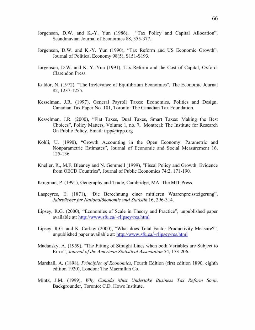
66

Jorgenson, D.W. and K.-Y. Yun (1986), “Tax Policy and Capital Allocation”, Scandinavian Journal of Economics 88, 355-377.

Jorgenson, D.W. and K.-Y. Yun (1990), “Tax Reform and US Economic Growth”,

Journal of Political Economy 98(5), S151-S193. Jorgenson, D.W. and K.-Y. Yun (1991), Tax Reform and the Cost of Capital, Oxford:

Clarendon Press. Kaldor, N. (1972), “The Irrelevance of Equilibrium Economics”, The Economic Journal

82, 1237-1255. Kesselman, J.R. (1997), General Payroll Taxes: Economics, Politics and Design,

Canadian Tax Paper No. 101, Toronto: The Canadian Tax Foundation. Kesselman, J.R. (2000), “Flat Taxes, Dual Taxes, Smart Taxes: Making the Best

Choices”, Policy Matters, Volume 1, no. 7, Montreal: The Institute for Research On Public Policy. Email: irpp@irpp.org

Kohli, U. (1990), “Growth Accounting in the Open Economy: Parametric and

Nonparametric Estimates”, Journal of Economic and Social Measurement 16, 125-136.

Kneller, R., M.F. Bleaney and N. Gemmell (1999), "Fiscal Policy and Growth: Evidence

from OECD Countries", Journal of Public Economics 74:2, 171-190. Krugman, P. (1991), Geography and Trade, Cambridge, MA: The MIT Press. Laspeyres, E. (1871), “Die Berechnung einer mittleren Waarenpreissteigerung”,

Jahrbücher fur Nationalökonomic und Statistik 16, 296-314. Lipsey, R.G. (2000), “Economies of Scale in Theory and Practice”, unpublished paper

available at: http://www.sfu.ca/~rlipsey/res.html Lipsey, R.G. and K. Carlaw (2000), “What does Total Factor Productivity Measure?”,

unpublished paper available at: http://www.sfu.ca/~rlipsey/res.html Madansky, A. (1959), “The Fitting of Straight Lines when both Variables are Subject to

Error”, Journal of the American Statistical Association 54, 173-206. Marshall, A. (1898), Principles of Economics, Fourth Edition (first edition 1890, eighth

edition 1920), London: The Macmillan Co. Mintz, J.M. (1999), Why Canada Must Undertake Business Tax Reform Soon,

Backgrounder, Toronto: C.D. Howe Institute.

67

Morrison, C. and W.E. Diewert (1990), “Productivity Growth and Changes in the Terms of Trade in Japan and the United States”, pp. 201-227 in Productivity Growth in Japan and the United States, C.R. Hulten (ed.), University of Chicago Press, Chicago.

Nakamura, A.O. and W.E. Diewert (2000), “Insurance for the Unemployed: Canadian

Reforms and their Relevance for the United States”, pp. 217-247 in Long-Term Unemployment and Reemployment Policies, L.J. Bassi and S.A. Woodbury (eds.), Stamford Connecticut: JAI Press.

Nakamura, A.O. and P. Lawrence (1994), “Education, Training and Prosperity”, John

Deutsch Institute for the Study of Economic Policy (March), 235-279. Nordhaus, W.D. (1969), “Theory of Innovations: An Economic Theory of Technological

Change”, American Economic Review 59 (May), 18-28. Paasche, H. (1874), “Über die Preisentwicklung der letzten Jahre nach den Hamburger

Borsennotirungen”, Jahrbücher fur Nationalökonomie und Statistik 12, 168-178. Pierson, N.G. (1896), “Further Consideration on Index Numbers”, Economic Journal 6,

127–131. Romer, P. (1994), “New Goods, Old Theory and the Welfare Costs of Trade

Restrictions”, Journal of Development Economics 43, 5-38. Samuelson, P.A. (1967), “The Monopolistic Competition Revolution”, In Monopolistic

Competition Theory: Studies in Impact, R.E. Kuenne (ed.), New York: John Wiley.

Smith, A. (1963), The Wealth of Nations, Volume 1 (first published in 1776),

Homewood, Illinois: Richard D. Irwin. The Economist (2000), “New Zealand’s Economy”, London, December 2. Tobin, J. (1956), “The Interest Elasticity of Transactions Demand for Cash”, The Review

of Economics and Statistics 38, 241-247. Törnqvist, L. and E. Törnqvist (1937), “Vilket är förhällandet mellan finska markens

ochsvenska kronans köpkraft?”, Ekonomiska Samfundets Tidskrift 39, 1-39 reprinted as pp. 121-160 in Collected Scientific Papers of Leo Törnqvist, Helsinki: The Research Institute of the Finnish Economy, 1981.

Walsh, B. (2000), “The Role of Tax Policy in Ireland’s Economic Renaissance”,

Canadian Tax Journal 48:3, 658-673.

68

Walsh, C.M. (1901), The Measurement of General Exchange Value, New York: Macmillan and Co.

Walsh, C.M. (1921a), The Problem of Estimation, London: P.S. King & Son. Walsh, C. M. (1921b), “Discussion”, Journal of the American Statistical Association 17,

537-544. Watson, W. (1999), “Labour Day, From the Front Porch”, Financial Post, Toronto,

Canada, September 8. Whitin, T.M. (1952), “Inventory Control in Theory and Practice”, Quarterly Journal of

Economics 66, 502-521. Whitin, T.M. (1957), The Theory of Inventory Management, Second edition, Princeton,

N.J.: Princeton University Press. Young, A.A. (1928), “Increasing Returns and Economic Progress”, Economic Journal

38, 527-542. Zeitsch, J. and D. Lawrence (1996), “Decomposing Economic Inefficiency in Base-Load

Power Plants”, The Journal of Productivity Analysis 7, 359-378.