THE MATHIEU DIFFERENTIAL EQUATION AND ...pi.math.cornell.edu/~rand/randpdf/mathieu_str.pdfThe...
59
THE MATHIEU DIFFERENTIAL EQUATION AND GENERALIZATIONS TO INFINITE FRACTAFOLDS SHIPING CAO 1 , ANTHONY CONIGLIO 2 , XUEYAN NIU 3 , RICHARD RAND 4 , AND ROBERT STRICHARTZ 5 Abstract. One of the more well-studied equations in the theory of ODEs is the Mathieu differential equation. Because of the difficulty in finding closed-form solutions to this equation, it is often necessary to seek solutions via Fourier series by converting the equation into an infinite system of linear equations for the Fourier coefficients. In this paper we present results pertaining to the stability of this equation and convergence of solutions. We also investigate ways to modify the linear-system form of the equation in order to study a wider class of equations. Further, we provide a method in which the Mathieu differential equation can be generalized to be defined on an infinite fractafold, with our main focus being the fractal blow-up of the Sierpinski gasket. We discuss methods for studying the stability of solutions to this fractal differential equation and describe further results concerning properties and behavior of solutions. Table of Contents 1. Introduction 2 2. Definitions and Methods 3 2.1. Background & Definitions 3 2.2. Fourier Expansion and Matrix Form 4 2.3. Truncation Method 6 2.4. Backward Recursion 7 3. Three-Term Recurrence Relations and Truncations of the Infinite Matrices 7 3.1. Asymptotic Behavior of {c j } ∞ j =1 7 3.2. The Truncation Method 10 4. Observations and Analysis for the Mathieu Differential Equation on the Line 12 4.1. The δ -ε Plot 12 4.2. Solutions of the Mathieu Differential Equation 15 4.3. Explanation on the Behavior of the Solutions 26 5. The Sierpinski Gasket and the Fractal Laplacian 29 5.1. Sierpinski Gasket 29 5.2. Fractal Laplacian 31 5.3. Spectral Decimation 32 5.4. Infinite Sierpinski Gasket 35 6. Extending the Mathieu Differential Equation to Infinite Fractafolds 36 6.1. Defining the Fractal MDE 36 6.2. Variants of the Mathieu Differential Equation on the Line 38 7. Ovservations and Analysis for the Fractal Mathieu Differential Equation 40 7.1. The δ -ε Plot 40 7.2. Solutions of the Mathieu Differential Equation 43 1 Cornell University, mathematics graduate student ([email protected]) 2 Indiana University Bloomington, class of 2019 ([email protected]) 3 University of Hong Kong, class of 2019 ([email protected]) 4 Professor of Mathematics, Cornell University ([email protected]) 5 Professor of Mathematics, Cornell University ([email protected]) 0 arXiv:1904.00950v1 [math.CA] 1 Apr 2019
Transcript of THE MATHIEU DIFFERENTIAL EQUATION AND ...pi.math.cornell.edu/~rand/randpdf/mathieu_str.pdfThe...

THE MATHIEU DIFFERENTIAL EQUATION ANDGENERALIZATIONS TO INFINITE FRACTAFOLDS
SHIPING CAO1, ANTHONY CONIGLIO2, XUEYAN NIU3, RICHARD RAND4,AND ROBERT STRICHARTZ5
Abstract. One of the more well-studied equations in the theory of ODEs is the Mathieu differentialequation. Because of the difficulty in finding closed-form solutions to this equation, it is often necessary
to seek solutions via Fourier series by converting the equation into an infinite system of linear equationsfor the Fourier coefficients. In this paper we present results pertaining to the stability of this equation
and convergence of solutions. We also investigate ways to modify the linear-system form of the equation
in order to study a wider class of equations. Further, we provide a method in which the Mathieudifferential equation can be generalized to be defined on an infinite fractafold, with our main focus
being the fractal blow-up of the Sierpinski gasket. We discuss methods for studying the stability of
solutions to this fractal differential equation and describe further results concerning properties andbehavior of solutions.
Table of Contents
1. Introduction 22. Definitions and Methods 3
2.1. Background & Definitions 32.2. Fourier Expansion and Matrix Form 42.3. Truncation Method 62.4. Backward Recursion 7
3. Three-Term Recurrence Relations and Truncations of the Infinite Matrices 73.1. Asymptotic Behavior of {cj}∞j=1 73.2. The Truncation Method 10
4. Observations and Analysis for the Mathieu Differential Equation on the Line 124.1. The δ-ε Plot 124.2. Solutions of the Mathieu Differential Equation 154.3. Explanation on the Behavior of the Solutions 26
5. The Sierpinski Gasket and the Fractal Laplacian 295.1. Sierpinski Gasket 295.2. Fractal Laplacian 315.3. Spectral Decimation 325.4. Infinite Sierpinski Gasket 35
6. Extending the Mathieu Differential Equation to Infinite Fractafolds 366.1. Defining the Fractal MDE 366.2. Variants of the Mathieu Differential Equation on the Line 38
7. Ovservations and Analysis for the Fractal Mathieu Differential Equation 407.1. The δ-ε Plot 407.2. Solutions of the Mathieu Differential Equation 43
1Cornell University, mathematics graduate student ([email protected])2Indiana University Bloomington, class of 2019 ([email protected])3University of Hong Kong, class of 2019 ([email protected])4Professor of Mathematics, Cornell University ([email protected])5Professor of Mathematics, Cornell University ([email protected])
0
arX
iv:1
904.
0095
0v1
[m
ath.
CA
] 1
Apr
201
9

Cao, Coniglio, Niu, Rand, and Strichartz 1
8. Further Research 549. Appendix 55References 57

Cao, Coniglio, Niu, Rand, and Strichartz 2
1. Introduction
The Mathieu differential equation, as will be defined in Section 2, takes the formd2udt2
+ (δ + ε cos t)u = 0, where δ, ε ∈ R are fixed, and u : R → R. Named after French
mathematician Emile Leonard Mathieu (1835-1890), the origin of the Mathieu differentialequation stems from real-world phenomena. For example, it describes the motion of apendulum subject to a periodic driving force. See [21] for more details.
One topic pertaining to the Mathieu differential equation which has been much re-searched is the stability of solutions. See [2, 10, 16, 17, 28]. Readers may also read[21, 18] for a brief introduction to this area. Most of the existing literature concernsthe parameter space, i.e. the space of δ-ε pairs, whose choices can drastically alter thebehavior of solutions. This paper presents research results and new phenomena both onthe parameter space and on solutions.
On the other hand, another area of mathematics which has been actively researchedin recent years is analysis on fractals, based on J. Kigami’s construction of Laplacians onpost-critically finite self-similar sets. See [13, 15, 14, 22]. It is of interest to define andstudy the Mathieu differential equation on fractal domains, and one suitable domain isthe infinite Sierpinski gasket developed by R.S. Strichartz [24]. Existing research on theinfinite Sierpinski gasket and on other ‘fractafolds’ be found in [12, 20, 23, 25, 26, 27].In particular, we will use the important result concerning the spectrum of the Laplacianon the infinite Sierpinski gasket by A. Teplyaev [27]. We will explore a way to generalizethe Mathieu differential equation to be defined on the infinite Sierpinski gasket.
This paper is organized as follows. In Section 2, we provide relevant background onthe Mathieu differential equation, give definitions which will be used throughout theremainder of the paper, and describe some of the methods used to study the relationshipthat the values of δ and ε have to the solutions of the equation; in doing so we willdiscuss ‘transition curves’ and the ‘truncation method’ used to study solutions to theMathieu differential equation. In Section 3 we present a number of proofs for theoremspertinent to the Mathieu differential equation and provide justification for the methodspresented in Section 2. Some of our methods and proofs are modified versions from[1, 9]. In Section 4 we provide a discussion of computational results in studying theMathieu differential equation, including results related to the asymptotic behavior oftransition curves and the convergence of solutions. In Section 5 we give an overview ofthe Sierpinski gasket (SG) and provide definitions of various terms in fractal analysis,such as the fractal Laplacian and the infinite Sierpinski gasket (SG∞), to be used inthe remaining sections. In Section 6 we extend the content of Sections 2, 3, and 4 tothe fractal setting by explaining how the ‘Mathieu differential equation defined on thereal line’ can be generalized to a ‘Mathieu differential equation defined on the infiniteSierpinski gasket.’ We describe how solutions to this generalization can be studied byconsidering solutions expanded as a linear combination of eigenfunctions of the fractalLaplacian. We also describe how the ‘truncation method’ on the line can be used tostudy the Mathieu differential equation on SG∞. In Section 7 we provide computationalresults and observations about the shape and asymptotic behavior of the transition curvesfor the Mathieu differential equation on SG∞ and also about the behavior of solutions.In Section 8 we describe further research that can be done on the Mathieu differentialequation and its fractal generalizations. Section 9, the Appendix, describes an alternateapproach to the ‘truncation method’ which involves partitioning Fourier coefficients intovarious equivalence classes.

Cao, Coniglio, Niu, Rand, and Strichartz 3
A website for this research has been created at http://pi.math.cornell.edu/∼aac254/.We invite the reader to visit this website, as it contains plots, graphs, data, and otherinformation gathered from the research.
2. Definitions and Methods
In this section we give formal definitions pertaining to the Mathieu differential equationon the real line and then describe the main methods used to study it.
2.1. Background & Definitions. We begin by defining the Mathieu differential equa-tion on the real line.
Definition 2.1 (Mathieu Differential Equation). The Mathieu differential equation (onthe real line) is defined as
d2u
dt2+ (δ + ε cos t)u = 0, (2.1)
where δ, ε ∈ R are fixed and u : R→ R is unknown.
Henceforth, the abbreviation ‘MDE’ will often be used to denote ‘Mathieu differentialequation.’ Also, unless otherwise specified, the term ‘Mathieu differential equation’ (andits abbreviation), when used in Sections 2, 3, and 4, will always refer to the MDE definedon the real line, as opposed to the later sections which discuss the MDE as defined on afractal domain.
The particular values of δ and ε chosen can drastically alter the corresponding solutionsto the MDE (see [21], for example). With this in mind, we make the following definition.
Definition 2.2 (Stable and Unstable δ-ε Pairs). (a). An ordered pair (δ, ε) ∈ R2 is astable pair of values if every solution to the corresponding MDE remains bounded for allt ∈ R.
(b). An ordered pair (δ, ε) ∈ R2 is an unstable pair of values if there exists a solutionto the corresponding MDE which is unbounded.
In order to understand which values of δ and ε correspond to stable pairs and whichcorrespond to unstable pairs, it is useful to examine the δ-ε plane given in Figure 2.1. Inthis figure, the horizontal axis is the δ-axis, and the vertical axis is the ε-axis. The grayshaded region of the plane corresponds to (δ, ε) pairs which are stable and is called thestable region; the white region of the plane corresponds to (δ, ε) pairs which are unstableand is called the unstable region. The solid curves and dashed curves which are eitherorange or black are called the transition curves and form the boundary between the stableregion and the unstable region. The curves which share the same color (either orange orblack) and the same format (either solid or dashed) share certain properties in commonwhich will be discussed in Section 2.2.
There exists a systematic method for determining the stable and unstable regions shownin Figure 2.1, which we describe in Section 2.2. A useful result regarding this method isgiven in [21] as follows:
Theorem 2.3. A pair (δ, ε) lies on a transition curve for the MDE if and only if thereexists a corresponding nontrivial solution u : R → R which is periodic with period 2π or4π.

Cao, Coniglio, Niu, Rand, and Strichartz 4
Figure 2.1. Stable and Unstable Regions of the δ-ε plane.
Theorem 2.3 motivates us to study the solutions to the MDE with Fourier series.
Remark 2.4. In this paper, we say f is periodic of period 2Nπ, or f is 2Nπ-periodic, ifN is the smallest positive integer such that f admits the Fourier expansion
f(t) =∞∑j=0
aj cos
(j
Nt
)+∞∑j=1
bj sin
(j
Nt
).
2.2. Fourier Expansion and Matrix Form. Let us suppose we have a periodic solu-tion u with period 2π or 4π to the Mathieu differential equation. In this case, we canwrite the Fourier series expansion of u as
u(t) =∞∑j=0
aj cos
(j
2t
)+∞∑j=1
bj sin
(j
2t
).
If we plug this Fourier series for u into the MDE, rearrange terms, and use sometrigonometric identities, we find that the function u given above solves the MDE if andonly if the two infinite systems of linear homogeneous equations shown below for thecosine and sine coefficients are satisfied. See [18] and [21] for more details.
cosine coefficients
δa0 + ε2a2 = 0,(
δ −(
12
)2)a1 + ε
2(a3 + a1) = 0,
(δ − 1)a2 + εa0 + ε2a4 = 0,(
δ −(j2
)2)aj + ε
2(aj−2 + aj+2) = 0, (j ≥ 3),
and
sine coefficients
(δ −
(12
)2)b1 + ε
2(b3 − b1) = 0,
(δ − 1)b2 + ε2b4 = 0,(
δ −(j2
)2)bj + ε
2(bj−2 + bj+2) = 0, (j ≥ 3).

Cao, Coniglio, Niu, Rand, and Strichartz 5
To solve these systems of equations, we consider putting them into matrix form. Read-ers can check that the above two systems of equations are equivalent to the following fourequations in matrix form collectively, which correspond to cosine or sine coefficients witheven or odd indexes. All the matrices are tridiagonal.
For the cosine coefficients with even indexes, we haveδ ε
2
ε δ − 12 ε2
ε2
δ − 22 ε2
ε2
δ − 32 ε2
. . . . . . . . .
︸ ︷︷ ︸
A
a0
a2
a4
a6...
︸ ︷︷ ︸aeven
=
0000...
︸ ︷︷ ︸
0
.
For the sine coefficients with even indexes, we haveδ − 12 ε
2ε2
δ − 22 ε2
ε2
δ − 32 ε2
. . . . . . . . .
︸ ︷︷ ︸
B
b2
b4
b6...
︸ ︷︷ ︸beven
=
000...
.
For cosine coefficients with odd indexes, we haveδ − 1
4+ ε
2ε2
ε δ − 94
ε2
ε2
δ − 254
ε2
ε2
δ − 494
ε2
. . . . . . . . .
︸ ︷︷ ︸
C
a1
a3
a5
a7...
︸ ︷︷ ︸aodd
=
0000...
.
For sine coefficients with odd indexes, we haveδ − 1
4− ε
2ε2
ε δ − 94
ε2
ε2
δ − 254
ε2
ε2
δ − 494
ε2
. . . . . . . . .
︸ ︷︷ ︸
D
b1
b3
b5
b7...
︸ ︷︷ ︸bodd
=
0000...
.
We can solve the above four matrix equations separately. If either of the first twoequations has a nontrivial solution in `2, then the MDE has a 2π-periodic solution, since
u(t) :=∑
j=0,2,4,6,...
aj cos
(j
2t
)+
∑j=2,4,6,...
bj sin
(j
2t
)solves the MDE and is 2π-periodic, comparing with Remark 2.4. Similarly, if either thethird or fourth equations has a nontrivial solution in `2, then the MDE has a 4π-periodicsolution, since
u(t) :=∑
j=1,3,5,...
aj cos
(j
2t
)+
∑j=1,3,5,...
bj sin
(j
2t
)

Cao, Coniglio, Niu, Rand, and Strichartz 6
solves the MDE and is 4π-periodic, also comparing with Remark 2.4. Interested readerscan also read the appendix for equations in matrix form for periodic solutions with largerperiods, say 2Nπ with N an arbitrary positive integer.
Now we return our discussion to Figure 2.1, where we plot the stable and unstableregions. According to Theorem 2.3, the transition curves consist of (δ, ε) pairs withnontrivial 2π- or 4π-periodic solutions. Equivalently, by the above discussion, (δ, ε) lieson a transition curve if and only if at least one of the four equations in matrix formdiscussed above has a nontrivial solution in `2. Since we develop four different equationsin matrix form, we use different colors (orange and black) and line formats (solid anddashed) in Figure 2.1 to distinguish between the four matrix equations:
• If (δ, ε) falls on a black solid line, then the equation Ax = 0 has a nontrivialsolution.
• If (δ, ε) falls on a black dashed line, then the equation Bx = 0 has a nontrivialsolution.
• If (δ, ε) falls on an orange solid line, then the equation Cx = 0 has a nontrivialsolution.
• If (δ, ε) falls on an orange dashed line, then the equation Dx = 0 has a nontrivialsolution.
2.3. Truncation Method. In finite-dimensional linear algebra, a homogeneous matrixsystem of equations Mx = 0, where M is an m ×m matrix, has a nontrivial solution ifand only if the determinant of M is zero. Although our four systems of matrix equationsabove are infinite, we hope to use techniques from finite-dimensional linear algebra tostudy the properties of these infinite systems.
For each infinite matrix, fix m ∈ N and consider its m×m leading principal submatrix.Below we give the truncated matrices Am and Bm of A and B, respectively, as examples.Cm and Dm are defined similarly.
Am =
δ ε2
ε δ − 12 ε2
ε2
δ − 22 ε2
ε2
δ − 32 ε2
. . . . . . . . .ε2
δ − (m− 1)2
Bm =
δ − 12 ε2
ε2
δ − 22 ε2
ε2
δ − 32 ε2
ε2
δ − 42 ε2
. . . . . . . . .ε2
δ −m2
Taking the determinant of each truncated matrix yields an algebraic expression involvingδ and ε. Setting each expression equal to zero, we can then plot each equation in theδ-ε plane and obtain a set of algebraic curves in the variables δ and ε. If we choose msufficiently large, the δ-ε curves derived from the truncated matrices will be very close tothe true transition curves corresponding to the infinite matrices. This statement is madeprecise by Ikebe et al. in [1], and we present their results in Section 3.2.

Cao, Coniglio, Niu, Rand, and Strichartz 7
2.4. Backward Recursion. In addition to studying the parameter space, it is also ofinterest to investigate the set of periodic solutions to the MDE. Motivated by the discus-sions in Section 2.2, we will study the Fourier coefficients of periodic solutions. For thecomputational results presented the paper, when numerically computing Fourier coeffi-cients of solutions, instead of computing a2, a4, a6,... successively given an initial value a0
(and similarly for the other three matrix equations) using the recursion relation on Page4, we will compute Fourier coefficients by setting initial value an0 for some large index n0
and compute an0−2, an0−4, an0−6,... successively. The former method is called the ‘forwardrecursion method’, whereas the latter method is called the ‘backward recursion method.’We choose to use the backward recursion method instead of the more commonly-usedforward recursion method due to the instability of the forward recursion method, whichwill be discussed in Section 3.1. Also see [9] for more details on the backward recursionmethod.
3. Three-Term Recurrence Relations and Truncations of the InfiniteMatrices
In this section, we will provide theoretical foundation for the methods we use. In doingso we will discuss the asymptotic convergence of Fourier coefficients and provide an errorestimate for the truncation method we use for approximating the transition curves. (Wewill extend these techniques to the fractal MDE in later sections.)
In this section, we work in generality by considering matrices of the formδ − λ1 − γε α1ε
β1ε δ − λ2 α2εβ2ε δ − λ3 α3ε
β3ε δ − λ4. . .
. . . . . .
, (3.1)
where αj, βj, λj ∈ R for j ≥ 1, and γ ∈ R; further, we assume that {αj}∞j=1 and {βj}∞j=1
are bounded sequences and that limj→∞ λj = ∞. Note that matrices A,B,C, and D asdefined in Section 2.2 are special cases of (3.1). In addition, we always assume αj, βj 6= 0,for all j ≥ 0, in this section. We will consider equations of the form
δ − λ1 − γε α1εβ1ε δ − λ2 α2ε
β2ε δ − λ3 α3ε
β3ε δ − λ4. . .
. . . . . .
c1
c2
c3
c4...
=
0000...
, (3.2)
where c = (c1, c2, · · ·)T ∈ `2 :={
(x1, x2, ...)T :∑∞
j=1 |xj|2 <∞
}is a real sequence.
3.1. Asymptotic Behavior of {cj}∞j=1. Three-term recurrence relations (TTRRs) anddifference equations have been well-studied throughout the last century. Since (3.2)naturally gives a TTRR,{
(δ − λ1 − γε)c1 + α1εc2 = 0,
βj−1εcj−1 + (δ − λj)cj + αjεcj+1 = 0, for j ≥ 2,(3.3)

Cao, Coniglio, Niu, Rand, and Strichartz 8
we can use existing theorems to study the asymptotic behavior of the sequence {cj}∞j=1
as j →∞. Below we first present the well-known Poincare Theorem (see [9]), also calledthe Poincare-Perron Theorem, which describes the asymptotic behavior of solutions togeneral TTRRs, and then we will see how the theorem applies to the equations above.
Theorem 3.1 (Poincare-Perron Theorem, [9]). For j ≥ 1, let cj+1+bjcj+ajcj−1 = 0 withlimj→∞ bj = b and limj→∞ aj = a. Let t1 and t2 denote the zeros of the characteristicequation t2 + bt + a = 0. Then, if |t1|6= |t2|, the difference equation has two linearlyindependent solutions {xn} and {yn} satisfying
limj→∞
xjxj−1
= t1, limj→∞
yjyj−1
= t2.
If |t1|= |t2|, then
lim supj→∞
|cj|1j = |t1|
for any nontrivial solution {cj} to the recurrence relation.
With this theorem in mind, we consider the TTRR
fjcj+1 + djcj + gj−1cj−1 = 0 (j ≥ 1), (3.4)
where {fj} and {gj} neither of which contains 0 as one of its terms, are uniformlybounded, and where |dj|→ ∞ as j →∞. Notice that, with our assumptions, the solutionof Equation 3.4 is uniquely determined by specifying the first two terms c1 and c2. We canderive the following proposition from the Poincare-Perron Theorem, adapting its proofdirectly from the proof of the Poincare-Perron Theorem in [9].
Proposition 3.2. Assume {fj} and {gj}, neither of which is equal to the zero sequence,are uniformly bounded, and assume that |dj|→ ∞ as j →∞. Then the TTRR (3.4) hastwo linearly independent solutions {xj} and {yj} satisfying
xjxj−1
∼ −gj−1
dj,
yjyj−1
∼ −dj−1
fj−1
.
Proof. The proof is modified directly from the proof for the Poincare-Perron Theoremin [9]. For convenience, we assume dj 6= 0 for any j, since otherwise we can consider the
TTRR defined for j ≥ M for some large M . Let cj =(∏j−1
i=1fidi
)cj. Then the TTRR
becomes
cj+1 + cj +fj−1gj−1
dj−1djcj−1 = 0.
By the Poincare-Perron theorem, there exists a pair of linearly independent solutions ofthis new recurrence, {xj} and {yj}, satisfying
limj→∞
xjxj−1
= 0, limj→∞
yjyj−1
= −1.
For j sufficiently large, xj does not vanish. Indeed, if xj0 = 0 for some j0 ∈ N then
the TTRR impliesxj0+2
xj0+1= −1, which cannot happen if j0 were sufficiently large (since

Cao, Coniglio, Niu, Rand, and Strichartz 9
xjxj−1→ 0). Similarly, for j sufficiently large yj does not vanish, for if yj0 = 0 for some
j0 ∈ N thenyj0yj0−1
= 0, which cannot happen for j0 sufficiently large (sinceyjyj−1→ −1).
Let H(1)j = xj/xj−1 and H
(2)j = yj/yj−1. Then
H(i)j+1H
(i)j +H
(i)j +
fj−1gj−1
dj−1dj= 0, i = 1, 2.
Multiplying each side by H(l)j , l 6= i, we get{
H(1)j+1H
(1)j H
(2)j +H
(1)j H
(2)j +
fj−1gj−1
dj−1djH
(2)j = 0,
H(2)j+1H
(2)j H
(1)j +H
(1)j H
(2)j +
fj−1gj−1
dj−1djH
(1)j = 0.
Subtracting one equation from the other, we obtain
H(1)j H
(2)j
(H
(1)j+1 −H
(2)j+1
)=fj−1gj−1
dj−1dj
(H
(1)j −H
(2)j
).
So, since
H(1)j ∼ 0 and H
(2)j ∼ −1,
we have
H(1)j =
fj−1gj−1
dj−1dj
1
H(2)j
H(1)j −H
(2)j
H(1)j+1 −H
(2)j+1
∼ −fj−1gj−1
dj−1dj.
Therefore,
xjxj−1
=
(∏j−1i=1
difi
)xj(∏j−2
i=1difi
)xj−1
= H(1)j
dj−1
fj−1
∼ −gj−1
dj,
and
yjyj−1
=
(∏j−1i=1
difi
)yj(∏j−2
i=1difi
)yj−1
= H(2)j
dj−1
fj−1
∼ −dj−1
fj−1
. �
Let {zj} be an arbitrary solution to the TTRR 3.4. We say {zj} is a minimal solutionof the TTRR if it obeys
zjzj−1∼ −gj−1
dj, and we say {zj} is a dominant solution of the
TTRR if it satisfieszjzj−1∼ −dj−1
fj−1. Note that limj→∞ zj = 0 if {zj} is a minimal solution
and limj→∞ zj =∞ if {zj} is a dominant solution.We can apply Proposition 3.2 to study Equation 3.3, since Equation 3.3 consists of an
equation for c1, c2 and a TTRR of the form 3.4.
Corollary 3.3. Assume ε 6= 0.(a). Equation 3.2 has a unique solution up to multiplication by a constant.(b). Let c = (c1, c2, c3, ...)
T be a nontrivial solution to Equation (3.2). If c ∈ `2, then
cj will decay with the asymptotic behaviorcjcj−1∼ βj−1ε
λj−δ . If c /∈ `2, then cj will diverge
with the asymptotic behaviorcjcj−1∼ λj−1−δ
αj−1ε.
Cao, Coniglio, Niu, Rand, and Strichartz 10
Proof. It is equivalent to studying Equation 3.3.(a). Given c1 ∈ R, we can solve c2, c3, · · · inductively, which gives us a solution to
Equation 3.3. In this way, any solution to Equation 3.3 is uniquely determined by c1.(b) Any solution c = {cj}∞j=1 can be written as a linear combination of {xj} and {yj}
as given in in Proposition 3.2, and hence there exist p, q ∈ R such that cj = pxj + qyjfor all j. Note that if q 6= 0 then {zj} is a dominant solution, and if q = 0 then {zj} is aminimal solution.
If {cj} ∈ `2 then limj→∞ cj = 0 and thus {cj} cannot be a dominant solution; thus, we
must have p = 0 and hencecjcj−1∼ βj−1ε
λj−δ . On the other hand, if {cj} /∈ `2 then p 6= 0 and
hencecjcj−1∼ λj−1−δ
αj−1ε.
�
Corollary 3.3 shows that there is a sharp contrast between the two possible types ofbehavior that a solution to Equation (3.2) can have. Since {αj} and {βj} are bounded se-quences, when (δ, ε) are fixed and properly chosen any solution {cj} to (3.2) will convergeto 0 very rapidly; otherwise, all nontrivial solutions will tend to infinity very fast.
If c1 ∈ R is an initial value which corresponds to a minimal solution, Proposition 3.2shows that numerically computing the solution with the forward recursion method is un-stable, since a small error in computation will lead to a dominant solution, in which {cj}explodes. On the other hand, the backward recursion method can give a good approxi-mation for a minimal solution. In [9], detailed discussions are given on this method, aswell as a corresponding error estimate. We briefly state the result here.
Proposition 3.4 ([9]). Fix a large N , and set cN+1 = 0, cN = 1. Compute cN−1, cN−2, · · · , c1
one-by-one backward with TTRR (3.4). If {xk} is an arbitrary minimal solution and {yk}is an arbitrary dominant solution, then {cj} satisfy
ckck−1
(xkxk−1
)−1
− 1 =rNrk−1
· 1− rk/rk−1
1− rN/rk−1
,
where rk = xkyk
and 1 ≤ k ≤ N .
3.2. The Truncation Method. In this part, we introduce the truncation method fordetermining which (δ, ε) pairs yield nontrivial solutions of (3.2). We start from theobservationδ − λ1 − γε α1ε
β1ε δ − λ2 α2εβ2ε δ − λ3 α3ε
β3ε. . . . . .. . .
= δI −
λ1 + γε −α1ε−β1ε λ2 −α2ε
−β2ε λ3 −α3ε
−β3ε. . . . . .. . .
= δI − T (ε),
where I is the identity matrix and the shorthand notation T (ε) is used in the last equality.Clearly, for a fixed ε, equation (3.2) has nontrivial solutions if and only if δ is an eigenvalueof T (ε).
The eigenvalue problem for infinite tridiagonal matrices has been widely studied. In[1], there is a result on the error between eigenvalues of the truncated matrices and thoseof the corresponding infinite matrix. We state the result in Theorem 3.5 below.

Cao, Coniglio, Niu, Rand, and Strichartz 11
Here we consider the infinite symmetric tridiagonal matrix T of the form
T =
d1 f1
f1 d2 f2
f2 d3 f3
f3. . . . . .. . .
,
where dn →∞ as n→∞ and {fn} bounded. Denote its n× n truncation by Tn, i.e.,
Tn =
d1 f1
f1 d2 f2
. . . . . . . . .
fn−1 dn
.
Theorem 3.5. ([1]) Let T and Tn (n ≥ 1) be given as above.(a). T has pure point spectrum.(b). If δ is a given simple eigenvalue of T , then there exists, for each n ∈ N, an eigenvalueln of Tn such that the sequence {ln}∞n=1 satisfies ln → δ as n→∞. For any such sequencethe error is given by
ln − δ =fn+1cncn+1
cTc(1 + o(1)),
where c = (c1, c2, · · ·)T ∈ `2 is an eigenvector corresponding to δ.
We can extend the above result to nonsymmetric tridiagonal matrices.
Theorem 3.6. Let T be an infinite tridiagonal matrix of the form
T =
d1 f1
g1 d2 f2
g2 d3 f3
g3. . . . . .. . .
,
where dn →∞ as n→∞, and {fn}∞n=1 and {gn}∞n=1 are bounded, positive, and nonzero.Let Tn be the n × n truncation of T . If δ is a given simple eigenvalue of T , then thereexists, for each n ∈ N, an eigenvalue ln of Tn such that the sequence {ln}∞n=1 satisfiesln → δ as n→∞. For any such sequence the error is given by
ln − δ =
√fn+1gn+1cncn+1∑∞
j=1 κjc2j
(1 + o(1)),
where κj :=√∏j−1
i=1gifi
and where c = (c1, c2, · · ·)T ∈ `2 is an eigenvector corresponding
to δ.
Proof. (a) Let
T ′ =
d1
√f1g1√
f1g1 d2
√f2g2√
f2g2 d3
√f3g3
√f3g3
. . . . . .
. . .
.

Cao, Coniglio, Niu, Rand, and Strichartz 12
We observe that
T =
κ1
κ2
κ3
. . .
· T ′ ·κ−1
1
κ−12
κ−13
. . .
.
It is clear that T ′ is a self-adjoint operator from `2 to `2 with pure point spectrum byTheorem 3.5.
Let
c′ = diag(κ−11 , κ−1
2 , · · ·)c = (κ−11 c1, κ
−12 c2, · · ·)T ,
where c = (c1, c2, · · ·)T . Clearly, the eigenvalue equation (δI − T )c = 0 holds if and onlyif (δI − T ′)c′ = 0 in a pointwise sense, where I is the identity transformation.
In addition, from Corollary 3.3 we deduce that there is a one-to-one correspondencebetween eigenvectors of T and T ′ in `2. Indeed, if c is an eigenvector of T in `2, we havec′jc′j−1
=κ−1j cj
κ−1j−1cj−1
∼ −√fj−1gj−1
djbecause
cjcj−1∼ −gj−1
djby Corollary 3.3, which implies c′ is
an eigenvector of T ′ in `2, and for the same reason if c′ ∈ `2 is an eigenvector of T ′ thenc = diag(κ1, κ2, · · ·)c′ is an eigenvector of T in `2.
Now, using Theorem 3.5 we deduce that there is a sequence of eigenvalues of thetruncated T ′n that converges to the eigenvalue δ of T ′ and hence of T , since T and T ′
have the same eigenvalues. In addition, noticing that, for each n ∈ N, Tn has the sameeigenvalue as T ′n, we see that there is a sequence of eigenvalues of Tn which converges toδ. Lastly, the error estimate comes by applying Theorem 3.5 to T ′ with the eigenvectorc′ = diag(κ−1
1 , κ−12 , · · ·)c. �
4. Observations and Analysis for the Mathieu Differential Equation onthe Line
The Mathieu differential equation has been an important topic in differential equationsdue to its numerous real-world applications. However, most of the existing work on theMDE focuses on theoretical analysis of the stable and unstable regions of the δ-ε plane,such as the asymptotic behavior of the transition curves, and there has not been muchcomputational work done on the stability curves as well as on the solutions to the Mathieudifferential equation. In this section, in addition to describing some of our theoreticalresults, we will explain our computational results on the intricate shape of the δ-ε curvesand on the converging behavior of the solutions.
4.1. The δ-ε Plot. In this part, we use the truncation method introduced in Section 2and Section 3 to study the δ-ε curves in more detail.
As discussed above, the transition curves are found via 2π-periodic and 4π-periodicFourier expansions of solutions. However, one might wonder what the curves would beif the same process is undertaken for Fourier expansions of larger periods, say periods8π, 16π, 32π, .... The answer is that curves corresponding to expansions of larger periodsin fact ”fill in” the stable regions whose boundary is obtained using the 2π- and 4π-periodic expansions. See Figure 4.1 for an illustration.
In fact, this “fill in” property remains valid for even larger periods, and a proof is givenbelow.

Cao, Coniglio, Niu, Rand, and Strichartz 13
Figure 4.1. Curves corresponding to expansions of larger periods: curveswith 2π-periodic solutions (black solid and black dashed), curves with4π-periodic solutions (orange solid and orange dashed), curves with 8π-periodic solutions (red dashed) and curves with 16π-periodic solutions (bluedashed).
Proposition 4.1. Let D be the set of δ-ε pairs such that the corresponding MDE has asolution of period 2kπ for some k ≥ 3. Then D is dense in the stable region.
Proof. First, if (δ, ε) is a stable pair, then by the discussion given in Chapter VI of [21]we can find two linearly independent solutions u1 and u2 of the MDE, such that(
u1(2π)u′1(2π)
)= ei2πθ
(u1(0)u′1(0)
),
(u2(2π)u′2(2π)
)= e−i2πθ
(u2(0)u′2(0)
),
for some θ ∈ [0, 12]. θ is uniquely determined by the pair (δ, ε), so we may view θ = θ(δ, ε)
as a function from the stable region to [0, 1/2].In fact, by the Floquet Theorem, there exists a 2×2 matrix A depending only on (δ, ε)
such that, for any solution u of the MDE,(u(t+ 2π)u′(t+ 2π)
)= A
(u(t)u′(t)
).
So (δ, ε) is a stable pair only if the two eigenvalues of A both have norm 1, which canbe written as ei2πθ and e−i2πθ. Readers can find details in [21]. Clearly, A dependscontinuously on the parameter (δ, ε), which shows that θ = θ(δ, ε) is a continuous functionon the stable region.
Next, we fix θ0 ∈ [0, 12] and ε ∈ R, and show that only countably many δ’s can be
found such that θ0 = θ(δ, ε). Recall that for each such δ we have a solution u1 to the

Cao, Coniglio, Niu, Rand, and Strichartz 14
corresponding MDE so that e−iθ0tu1(t) is a 2π-periodic function. We have the Fourierseries expansion e−iθ0tu1(t) =
∑∞j=−∞ cje
ijt, which implies
u1(t) = eiθ0t∞∑
j=−∞
cjeijt.
Plugging this into the Mathieu differential equation, we get the following equation forthe coefficients,
. . . . . . . . .
δ − (θ0 − 2)2 ε2
ε2
δ − (θ0 − 1)2 ε2
ε2
δ − θ20
ε2
ε2
δ − (θ0 + 1)2 ε2
. . . . . . . . .
...c−2
c−1
c0
c1
c2...
=
...00000...
.
From this we can see that there are only countably many values of δ such that thecorresponding equation has a nontrivial solution {cj}∞j=−∞ ∈ {c ∈ CZ|
∑∞j=−∞|cj|2<∞}.
Now, we prove the proposition by contradiction. Suppose D is not dense in the stableregion. Then, there is a ball in the δ-ε plane where θ does not take any dyadic rationalvalue, noticing that when θ is a dyadic rational the MDE has 2kπ-periodic solutions u1, u2
for some k. This means θ equals a constant θ0 on that ball, since θ is a continuous functionof (δ, ε). However, for this fixed θ = θ0, and a fixed ε in the ball, there are only count-ably many possible values for δ, which can not fill in the ball. This gives a contradiction.�
Next we will discuss the asymptotic behavior of the stable and unstable regions. Ex-isting works including [10], [16], and [28] cover two important observations:
(i) First, as illustrated in Figure 4.2, the width of each stable band gets thinner andthinner as |ε| tends to ∞. In [28], it is shown that the width of the kth stableband will decrease exponentially on |ε|≥ k2 as |ε|→ ∞.
(ii) Secondly, for each fixed ε, the width of kth unstable band becomes smaller ask increases. An estimate is given in [2] and [10] with different methods, bothyielding
dk =2|ε|k
2m((k − 1)! )2
(1 + o
(|ε|2
k2
)),
where dk is the width of the kth unstable band with ε fixed.
Since the study of the type of convergence in the second observation is comparativelycomplete, we focus on the type in the first observation, which concerns the width of thestable band as |ε|→ ∞. In particular, we study the first ten stable bands by computingthe width of each band from ε = 0 to ε = 50 in increments of 0.1. A graph for eachstable band, plotting width vs epsilon, are shown below. Then we use the curve fittingtoolbox in MATLAB to estimate the fitting curves between ε and width in each stableband. Please see Figure 4.3 and Figure 4.4 for the result and fitting curves.
The last topic we will discuss before moving on to talk about solutions to the MDE isto approximate and simplify the irregular boundary between stable and unstable regions

Cao, Coniglio, Niu, Rand, and Strichartz 15
Figure 4.2. The width of the 5th stable band.
for practical use. We can see that most (δ, ε) pairs in the first and the fourth quadrantswhich lie below by the line ε = δ and above by the line ε = −δ are stable, while most(δ, ε) values in those quadrants outside that region form unstable pairs. For any w > 0,let Rw := {(δ, ε) ∈ R2 : 0 < ε < w and − δ < ε < δ}. We are interested in determiningthe probability, for various values of w, that a δ-ε pair is stable, given that it lies in thetriangle Rw.
So, we numerically compute the probabilities with different choices of w. Notice thatthe line ε = δ (as well as the line ε = −δ) alternatively passes through stable and unstableregions. So, we define wi to be the δ-coordinate of the point of intersection between theline ε = δ and the right boundary of the i-th unstable region; also, for each i, we definePi to be the probability that a δ-ε pair is stable, given that it is in Rwi
. Readers can seefigure 4.5 for an illustration of how we divide the regions into triangles.Pi can also be considered as the probability of getting a stable (δ, ε) pair within the
triangular regions, which can characterize how well the irregular boundaries can be ap-proximated by lines ε = ±δ. We list the Pi, 1 ≤ i ≤ 18 in Table 1.
In addition, we also obtain a surprisingly good fitting curve of the form Pi = ai+bi+c
, witha = 0.9938, b = −0.1424, c = 0.3608. See figure 4.6 for details.
4.2. Solutions of the Mathieu Differential Equation. Now we discuss the periodicsolutions for the Mathieu differential equation. In Corollary 3.3, we showed that thesequence {cj} of Fourier coefficients to periodic solutions corresponding to δ-ε pairs on thetransition curves converge rapidly. Hence, given a δ-ε pair on a transition curve, we cancalculate explicitly the coefficients of the corresponding solution with a finite truncationof the Fourier series and use those coefficients to plot, with very high accuracy, solutionsto the MDE.
One question one might investigate is as follows. Suppose one fixes a transition curveand considers periodic solutions corresponding to various (δ, ε) points along that transi-tion curve. How do properties of solutions change as ε varies?
To be more precise, we need some new notation. Recall from Section 2.2 that, whensolving 2π- or 4π- periodic solutions, we can rewrite the MDE as a system of linearequations for Fourier coefficents, which collectively can be rewritten as four independent

Cao, Coniglio, Niu, Rand, and Strichartz 16
Fitting curve of the form: ab+ecx
.
1st stable band, a = 0.2278, b = −0.09431, c = 1.994
2nd stable band, a = 1.390, b = 0.8504, c = 1.24
3rd stable band, a = 6.045, b = 3.674, c = 0.9081
4th stable band, a = 20.17, b = 2.507, c = 0.6972
5th stable curve, a = 56.06, b = 23.20, c = 0.5527
Figure 4.3. The width of first 5 stable bands.

Cao, Coniglio, Niu, Rand, and Strichartz 17
Fitting curve of the form: ab+ecx
.
6th stable band, a = 136.8, b = 12.38, c = 0.4496
7th stable band, a = 303.0, b = 20.39, c = 0.374
8th stable band, a = 623.9, b = 164.2, c = 0.3168
9th stable band, a = 1212, b = 283.9, c = 0.2726
10th stable curve, a = 2248, b = 473.9, c = 0.2377
Figure 4.4. The width of 6th-10th stable bands.

Cao, Coniglio, Niu, Rand, and Strichartz 18
(a) Rw1(b) Rw2
(c) Rw3 (d) Rw4
Figure 4.5. The triangle area corresponding to Rw1 , Rw2 , Rw3 , and Rw4 .The green area is the stable region, and shaded area is the unstable region.
homogeneous matrix equations, with corresponding matrices A,B,C,D. The transitioncurves consist of the δ-ε pairs such that one of these matrices degenerates. In this way,a transition curve can be labeled with a matrix and an integer k ≥ 1, so that for eachδ-ε pair on this transition curve, δ is the kth smallest real number such that the matrixdegenerates with the fixed ε. We want a more convenient way to label these transitioncurves, and to achieve this, we proceed as follows. Fix a transition curve, let ε = 0 onthe transition curve, and solve the corresponding equation in matrix form. According tothe discussion in Section 2.2, we can then construct a periodic solution to the MDE, andthe solution is clearly an eigenfunction of d2
dt2. For example, if we consider the transition
curve labeled by A and k = 2 we will get cos t as a solution with the above process. Inthis way, a transition curve can be labeled with an eigenfunction of d2
dt2. In light of this,
we define p(ϕ, ε) to be the point in the δ-ε plane with prescribed ε-coordinate which lieson the transition curve corresponding to the eigenfunction ϕ.

Cao, Coniglio, Niu, Rand, and Strichartz 19
Table 1. The probability Pi’s.
i Pi1 0.6250564363874452 0.7844284258135943 0.8451396639958684 0.8781437877046725 0.8991545892320866 0.9138000567791797 0.9246325805975668 0.9329888586164579 0.93964086014742110 0.94506730076365711 0.94958160365015612 0.95339796028936213 0.95666792544324014 0.95950214042468515 0.96198296867162016 0.96417400634646517 0.96613354758969218 0.967239011961280
Figure 4.6. Probabilities Pi and the fitting curve.
As shown in Section 2, the transition curves can be organized into four different classes,made up of points {p(sin kt, ε)}, {p(cos kt, ε)}, {p(sin 2k+1
2t, ε)}, {p(cos 2k+1
2t, ε)} with our
new notation. It is natural to study them separately.First we consider the class {p(sin kt, ε)}. Because of the symmetry of the transition
curves across the δ-axis, it suffices to only consider positive values of ε. In fact, if u is a so-lution corresponding to the pair (ε, δ), then u(t+π) is a solution corresponding to the pair(−ε, δ) since − cos t = cos(t+π). The normalized solutions are plotted in Figures 4.7-4.9,

Cao, Coniglio, Niu, Rand, and Strichartz 20
where by ‘normalized solution’ we mean a solution u for which maxt∈R u(t) = 1. In plot-ting the graphs we have used the particular values k = 1, 2, 3 and ε = 5, 10, 20, 40, 80, 160.15× 15 truncated matrices are used to compute the solutions. The horizontal axis is thet-axis, and the vertical axis is the u-axis.
Figure 4.7. Normalized solutions corresponding to p(sin t, 0) (solidblack), p(sin t, 5) (red), p(sin t, 10) (orange), p(sin t, 20) (green), p(sin t, 40)(blue), p(sin t, 80) (purple).
Figure 4.8. Normalized solutions corresponding to p(sin 2t, 0) (solidblack), p(sin 2t, 5) (red), p(sin 2t, 10) (orange), p(sin 2t, 20) (green),p(sin 2t, 40) (blue), p(sin 2t, 80) (purple).
Figure 4.9. Normalized solutions corresponding to p(sin 3t, 0) (solidblack), p(sin 3t, 5) (red), p(sin 3t, 10) (orange), p(sin 3t, 20) (green),p(sin 3t, 40) (blue), p(sin 3t, 80) (purple).
An interesting pattern can be observed from Figure 4.7. The sequence of t-coordinatesof these maximal points appears to approach 0 monotonically as ε increases. Figures 4.8and 4.9 show the same behavior as well.
We now use curves to fit a curve of the t-coordinate of these relative maxima in [0, π]as a function of ε. We still pick the same three transition curves, and take ε from 1 to200, in increments by 1. The relationship of t coordinate of maximal points and ε on thethree curves are shown in figure 4.10, and the fitting curve is of the form t = aε+b
ε2+cε+d.
For the case of p(sin 2t, ε) and p(sin 3t, ε), does the same convergence behavior occur ifone considers the sequence of the first minima when t > 0? We also do the computation,and show the results in figure 4.11, where the same kind of fitting curve also works.

Cao, Coniglio, Niu, Rand, and Strichartz 21
t-position of maximal point on curve p(sin t, ε), witha = 3.031, b = 5.736, c = 10.18, d = 14.88.
t-position of maximal point on curve p(sin 2t, ε), witha = 10.31, b = 22.8, c = 17.43, d = 29.09.
t-position of maximal point on curve p(sin 3t, ε), witha = 432.5, b = 1345, c = 607.2, d = 1257.
Figure 4.10. t-position of maximal points, with fitting curve t = aε+bε2+cε+d
.
In case of p(sin 3t, ε), the same observation applies to the second maxima when t > 0.See figure 4.12 for details.
One can also consider the behavior of the u-coordinate of these various sequences oflocal extrema. See figure 4.13 for the behavior of u-coordinate of the first minimal pointson the curve p(sin 2t, ε), where we can fit the points well with a rational function of the
form aε2+bε+cε2+bε+c
.For the curve p(sin 3t, ε), there are three local extremes on each solution, and we also
do the computation for the u-coordinate for the first minimal and the second maximalvalue. The fitting curve is a little more complicated, of the form t = aε3+bε2+cε+d
ε3+dε2+eε+g. See
figure 4.14.Next, we turn to the solutions on curves p(cos kt, ε), and we do experiments for k =
0, 1, 2. Please look at figure 4.15,4.16,4.17 for the results.We can see that the shapes of these curves are different from those in figure 4.7 4.8,4.9.
The first curve p(cos 0t, ε) is of course very special, as it corresponds to the constantfunctions. It turns out the solution is always positive on this curve, as a consequence ofSturm’s Theorem [17]. Also, we have the minimal values of the solutions at π, see figure

Cao, Coniglio, Niu, Rand, and Strichartz 22
t-position of the second maximal point on curve p(sin 2t, ε), witha = 2.272, b = 4.602, c = 12.75, d = 19.84.
t-position of the second maximal point on curve p(sin 3t, ε), witha = 710.8.5, b = 1894, c = 5324, d = 1.045× 10⁴.
Figure 4.11. t-position of the second maximal points, with fitting curvet = aε+b
ε2+cε+d.
Figure 4.12. t-position of the third maximal points on curve p(sin 3t, ε),with fitting curve t = aε+b
ε2+cε+d, a = 9.567, b = 23.07, c = 22.86, d = 40.46.
Figure 4.13. u-position of the second maximal points on curve p(sin 2t, ε),
with fitting curve t = aε2+bε+cε2+dε+e
. a = 0.8393, b = −0.5638, c = 5.566, d =−0.1973, e = 5.571.
4.18 for the minimal values for different choices of ε. We use a fitting curve of the formu = aε+b
ε2+cε+d.

Cao, Coniglio, Niu, Rand, and Strichartz 23
u-position of the second maximal point on curve p(sin 3t, ε), witha = 0.7784, b = −3.71, c = 21.57, d = 150, e = −3.899, f = 30.57, g = 149.9.
u-position of the third maximal point on curve p(sin 3t, ε), witha = 0.8166, b = −4.106, c = 20.44, d = 136.9, e = −4.234, f = 25.11, g = 136.8.
Figure 4.14. u-position of the second and third maximal points corre-sponding to curve p(sin 3t, ε), with fitting curve u = aε3+bε2+cε+d
ε3+eε2+fε+g.
Figure 4.15. Normalized solutions corresponding to p(cos 0t, ε), with ε =0, 1, 2, 3, 4, 5, 10, 20, 40, 80, 160.
Figure 4.16. Normalized solutions corresponding to p(cos t, ε), with ε =0, 1, 2, 3, 4, 5, 10 in the left graph, and ε = 10, 20, 40, 80, 160 in the rightgraph.
The solutions on the second curve is a little more complicated. As shown in figure 4.16,we can see that minimal value is achieved at t = π in [0, 2π] for ε = 0 and ε = 1, butas ε becomes larger, the minimum point splits into two different minimum points. This

Cao, Coniglio, Niu, Rand, and Strichartz 24
Figure 4.17. Normalized solutions corresponding to p(cos 2t, ε), with ε =0, 1, 2, 3, 4, 5, 6 in the left, and ε = 6, 7, 8, 9, 10, 20, 30, 40, 60, 80, 100, 160 inthe right.
Figure 4.18. The u coordinate of minimum points of solutions for pointsp(cos 0, ε), with ε = 0, 1, · · · , 200. Fitting curve u = aε+b
ε2+cε+d, with a =
−0.02171, b = 0.2895, c = 0.2289, d = 0.2895.
is an interesting phenomenon, and we have an explanation for this in Theorem 4.4. Wedo computations on the t-coordinate of the minimum points as ε gets larger. Please seefigure 4.19 for the data, and we use a fitting curve of the form t = aε+b
ε2+cε+d.
Figure 4.19. The t coordinate of minimum points of solutions for pointsp(cos t, ε), with ε = 2, · · · , 200. Fitting curve y = aε+b
ε2+cε+d, with a =
241, 9, b = 1284, c = 310.8, d = 177.1.
Another thing we need to highlight here is that the maximal absolute value does notoccur at 0 or π, but at some other points. So, as usual, we normalize the solutions sothat their minimum value are −1, and we compute values of solutions at the two otherlocal peaks at 0 and π, which is shown in figure 4.20. It is also interesting to see in figure4.21 that the local maximal value at 0 drop rapidly near ε = 0, and then increase quickly.
The solutions on the curve p(cos 3t, ε) is even more complicated. Still, we observethe split of one peak. When ε = 0, 1, 2, 3, 4, 5, we only see one maximum point, but as εbecomes larger, we see two maximum points. We also do computation on the t coordinateof one of these splited maximum point. See figure 4.22 for the computation result, wherewe use fitting curves of the form t = aε2+bε+c
ε2+dε+e.

Cao, Coniglio, Niu, Rand, and Strichartz 25
Figure 4.20. The u coordinate of minimum points of solutions for pointsp(cos t, ε), with ε = 0, 1, 2, · · · , 200. Fitting curve u = aε2+bε+c
ε2+dε+e, with a =
0.8687, b = −1.631, c = 0.8498, d = −1.72 and e = 0.8497.
Figure 4.21. The u coordinate of minimum points of solutions for pointsp(cos t, ε), with ε = 0, 1, 2, · · · , 200. Fitting curve u = aε+b
ε2+cε+d, with a =
0.2495, b = −4.991, c = −3.037, d = 6.722.
Figure 4.22. The t coordinate of maximum points of solutions for pointsp(cos 2t, ε), with ε = 5, 6, · · · , 200. Fitting curve t = aε2+bε+c
ε2+dε+e, with a =
0.5572, b = 88.5, c = −3.009, d = 55.35 and e = −157.7.
We also do experiment on the t coordinate of the first minimum points and the u-coordinate of the peaks on the curve p(cos 2t, ε).
Figure 4.23. The t coordinate of the second peak of solutions for pointsp(cos 2t, ε), with ε = 5, 6, · · · , 200. Fitting curve t = aε2+bε+c
ε3+dε2+eε+f, with
a = 269.3, b = 4745, c = −9715, d = 641.3, e = −2040 and f = −6017.

Cao, Coniglio, Niu, Rand, and Strichartz 26
Figure 4.24. The t coordinate of the second peak of solutions for pointsp(cos 2t, ε), with ε = 1, 2, · · · , 200. Fitting curve t = aε3+bε2+cε+d
ε3+eε2+fε+g, with
a = 0.7931, b = −4.642, c = 6.596, d = 13.45, e = −− 5.508, f = 9.829 andg = 13.44.
Figure 4.25. The t coordinate of the second peak of solutions for pointsp(cos 2t, ε), with ε = 1, 2, · · · , 200. Fitting curve y = aε2+bε+c
ε2+eε+f, with a =
−0.006875, b = 0.7009, c = −8.537, d = −2.457, e = 8.857.
Figure 4.26. The t coordinate of the second peak of solutions for pointsp(cos 2t, ε), with ε = 5, 6, · · · , 200. Fitting curve y = aε2+bε+c
ε3+dε2+eε+f, with
a = 0.2268, b = −25.1, c = 587.7, d = 4.775, e = −156 and f = 1002.
4.3. Explanation on the Behavior of the Solutions. Before the end of this section,we give a proof on the convergence of the t-coordinates of the peaks. This interestingpoint is that the behaviors are closely related to the asymptotic behavior of the transitioncurves, i.e. how δ behaves as ε increases to ∞. There are several works on this problem,and here we refer [17] for one version. Readers can find other dicussions in [28].
Theorem 4.2 (W.S. Loud). For fixed ε > 0, let δ be the kth smallest value on thetransition curves. Then we have
δ = −ε+ (k − 1
2)√
2ε+O(ε1/2),
as ε→ +∞.

Cao, Coniglio, Niu, Rand, and Strichartz 27
Figure 4.27. Normalized solutions corresponding to p(sin 12t, ε), with ε =
0, 1, 2, 3, 4, 5, 10, 20, 40, 80, 160.
Figure 4.28. Normalized solutions corresponding to p(sin 32t, ε), with ε =
0, 5, 10, 20, 40, 80, 160.
Figure 4.29. Normalized solutions corresponding to p(cos 12t, ε), with ε =
0, 1, 2, 3, 4, 5, 10, 20, 40, 80, 160.
Figure 4.30. Normalized solutions corresponding to p(cos 32t, ε), with ε =
0, 1, 2, 3, 4, 5, 10, 20, 40, 80, 160.
Notice that in the above theorem, we fix a transition curve and let ε → ∞, which isexactly the way we study the behavior of the solutions. Now, we apply the theorem toderive some interesting facts that we have observed in our experiments.
Lemma 4.3. For fixed ε > 0, let δ be the kth smallest value on the transition curves,and u be a nontrivial periodic solution for the corresponding MDE. Then, for large ε > 0,there is no local extremum of u in [cε, π) where cε ∼ ε−1/4.

Cao, Coniglio, Niu, Rand, and Strichartz 28
Proof. Let cε be the zero of δ + ε cos t in (0, π), where theorem 4.2 guarantee theexistence of cε when ε is large. In addition, we have the estimate by using Taylor expansionof cos t locally at 0,
limε→∞
cεε1/4
= (2k − 1)12 2
34 .
We will show u′(t) 6= 0 on [cε, π), which immediately implies the lemma.First, we show there is no t ∈ [cε, π) such that u(t)u′(t) > 0, by contradiction. Without
loss of generality, we assume u(t0) > 0 and u′(t0) > 0 for some t0 ∈ [cε, π). Then wecan show that u(t) > 0, u′(t) > 0 for any t ∈ [t0, π]. If this is not true, we can taket1 = inf{t ∈ [t0, π] : u(t) ≤ 0 or u′(t) ≤ 0}, then u(t) and u′(t) are both increasing on[t0, t1] as {
ddtu = u′,
ddtu′ = −(δ + ε cos t)u,
where −(δ + ε cos t) > −(δ + ε cos cε) = 0 on (cε, π). As a consequence, u(t1) > 0 andu′(t1) > 0, which contradicts the definition of t1, noticing that both u, u′ are continuous.As a result, we see that u(t) > 0, u′(t) > 0 for any t ∈ [t0, π]. On the other hand, u satisfiesthe boundary condition u(π) = 0 or u′(π) = 0, since u takes a Fourier series expansionin one of the following forms (see [21]):
∑∞j=0 cj cos jt,
∑∞j=1 cj sin jt,
∑∞j=0 cj cos 2j+1
2t or∑∞
j=0 cj sin 2j+12t. This gives a contradiction.
Using the above observation, we can see u′(t) 6= 0 for any t ∈ [cε, π). Otherwise, ifu′(t) = 0 for some t ∈ [cε, π), we should have u(t) 6= 0, so that u(t + h)u′(t + h) > 0 forsome small h > 0. �
Theorem 4.4. (a). Consider a fixed transition curve characterized by the solution u(t) =sin kt or u(t) = cos(k+ 1
2)t. Fix a large ε > 0, and let u be a nontrivial periodic solution.
Then, we have all the local extremums of u in⋃n∈Z(−cε + 2nπ, cε + 2nπ), where cε tends
to 0 as ε→∞. (cε depends on k)(b). Consider a fixed transition curve characterized by the solution u(t) = cos kt or
u(t) = sin(k + 12)t. Fix a large ε > 0, and let u be a nontrivial periodic solution. Then,
we have all the local extremums of u in πZ∪ (⋃n∈Z(−cε+ 2nπ, cε+ 2nπ)), where cε tends
to 0 as ε→∞. (cε depends on k)In addition, there is a critical value α ≥ 0 given by the equation
δ − ε = 0,
where we view δ as a function of ε on a fixed transition curve. Then π is a local maximumof |u| if 0 ≤ ε < α, and π is a local minimum of |u| is ε > α. When ε = α and the curveis not characterized by cos 0t = 1, π is a local maximum of |u|.
Proof. (a) Lemma 4.3 shows that there are no local extremums in [cε, π). By symmetry,we do not have local extremums in
⋃n∈Z[cε, 2nπ + π)∪ (2nπ + π, cε]. It remains to show
(2k + 1)π, k ∈ Z are not local extremums in these cases. It is enough to show that π isnot a local extremum.
Note that for any case in part (a), a nontrivial 2π- or 4π-periodic solution u corre-sponding to a point (δ, ε) on a transition curve is written as a sum of sines or as a sumof cosines: u(t) =
∑∞k=0 ak sin(kt) or u(t) =
∑∞k=0 ak cos(k + 1
2)t.
It is easy to see that u(π) = 0. We therefore conclude that u′(π) 6= 0, since otherwiseu would be the trivial solution. As a result, π is not a local extremum.

Cao, Coniglio, Niu, Rand, and Strichartz 29
(b) We only need to understand the behavior of u at π. The idea is essentially thesame as the proof of Lemma 4.3, where we look at the sign of δ + ε cos t. It is also clearthat u(π) 6= 0 and u′(π) = 0 in this case.
Notice that u′′(π) = −(δ − ε)u(π), and we set u(π) > 0 by multipling a constant, sothat we can conveniently look at the absolute value of u. If δ + ε cos π = δ − ε > 0, thenπ is a local maximum of |u|; if δ − ε < 0, then π is a local minimum of |u|. For the casethat ε = δ, we can see that δ − ε cos t > 0 on (0, 2π) \ {π} except for the case δ = ε = 0,which only happens on the curve characterized by cos 0t. So π is still a local maximumof |u|.
In addition, δ − ε is a strictly decreasing function of ε on (0,∞), so we can find acritical point α such that δ − ε > 0 on (0, α), and δ − ε < 0 on (α,∞). To show thatδ − ε is strictly decreasing, notice that δ is the kth smallest value such that the MDEhas a 2π- or 4π-periodic solution, which is equivalent to say that δ is the kth smallesteigenvalue of the self-adjoint operator −∆ − ε cos t on L2(R/4πZ). Let ε > ε′ > 0, andδ, δ′ be the corresponding eigenvalues. Then using Raleigh quotient, we get
δ′ = maxu∈Mk,ε′
〈(−∆− ε′ cos t)u, u〉L2(R/4πZ)
‖u‖L2(R/4πZ)
> maxu∈Mk,ε′
〈(−∆− ε′ cos t− (ε− ε′)(cos t+ 1))u, u〉L2(R/4πZ)
‖u‖L2(R/4πZ)
= maxu∈Mk,ε′
〈(−∆− ε cos t)u, u〉L2(R/4πZ)
‖u‖L2(R/4πZ)
− (ε− ε′)
> infM
maxu∈M
〈(−∆− ε cos t)u, u〉L2(R/4πZ)
‖u‖L2(R/4πZ)
− (ε− ε′) = δ − (ε− ε′),
where Mk,ε′ is the space spanned by the smallest k eigenfunctions of −∆ − ε′ cos t andthe infimum in the last line is taken over all the k dimensional subspaces of dom∆ onR/4πZ. �
Remark. In Theorem 4.2, Lemma 4.3 and Theorem 4.4, we considered the case thatε ≥ 0. Since − cos t = cos(t+ π), for the case that ε ≤ 0, the MDE can be rewritten as
d2
dt2u+ (δ − ε cos t)u = 0,
with u(t) = u(t−π). We can still use Theorem 4.2, Lemma 4.3 and Theorem 4.4 to studysolutions to the MDE with coefficient ε < 0, by applying a shift of π.
5. The Sierpinski Gasket and the Fractal Laplacian
In this section we give preliminary definitions and results concerning analysis on fractalsand provide a basic introduction to the ‘infinite’ Sierpinski gasket will be given. Thisserves to set up the discussion of the generalization of the MDE to the fractal settingdescribed in in Section 6.
5.1. Sierpinski Gasket. Consider the three contraction mappings {Fi : R2 → R2}i=0,1,2
given by F0(x) = 1
2x
F1(x) = 12x+
(12, 0)
F2(x) = 12x+
(14,√
34
),

Cao, Coniglio, Niu, Rand, and Strichartz 30
where x ∈ R2. Then {Fi}i=0,1,2 form an ‘iterated function system’ (see page 133 of [7]).By Theorem 9.1 in [7], there exists a unique nonempty compact set K ⊂ R2 such that(see [11])
K =2⋃i=0
Fi(K).
Then K is defined to be the Sierpinski gasket, often denoted SG. See Figure 5.1.
Figure 5.1. The Sierpinski Gasket
In studying SG it is useful to use its graph approximations, constructed as follows. Letq0, q1, and q2 be the unique fixed points of F0, F1, and F2, respectively. Define a vertexset V0 := {q0, q1, q2} ⊂ SG. Then Fi(SG) ∩ Fj(SG) = FiV0 ∩ FjV0,for any i 6= j. Werefer to V0 as the boundary of SG. We further define vertex sets Vn ⊂ SG for n ≥ 1inductively by Vn :=
⋃2i=0 Fi(Vn−1) and let V∗ :=
⋃∞n=0 Vn be the set of all vertices. Note
that V∗ is dense in SG. For an m-tuple w = (w1, w2, · · · , wm), where wj ∈ {0, 1, 2} foreach wj (1 ≤ j ≤ m), we define Fw by
Fw := Fw1 ◦ Fw2 ◦ · · · ◦ Fwm
and say that w is a word of length |w| = m. With this, an edge relation ∼m on Vm canbe introduced as follows: for x, y ∈ Vm we say x ∼m y if and only if there exists a wordw of length m and unequal indices i, j ∈ {0, 1, 2} such that x = Fw(qi) and y = Fw(qj).This relation on Vm gives a sequence of graphs Γm approximating SG, with the vertexset Vm and the edge set Em = {{x, y}|x ∼m y}. See Figure 5.1 for Γ0,Γ1,Γ2.
Figure 5.2. Approximating graphs Γ0,Γ1,Γ2

Cao, Coniglio, Niu, Rand, and Strichartz 31
5.2. Fractal Laplacian. Now we are ready to define the Laplacian on SG. Supposeu : SG→ R. We define the level-m discrete Laplacian ∆m by
∆mu(x) :=∑y∼mx
(u(y)− u(x)), x ∈ Vm \ V0.
Then we define the continuous Laplacian ∆ by
∆u(x) =3
2limm→∞
5m∆mu(x), x ∈ V∗ \ V0.
If the limit above converges uniformly on V∗ \ V0 to a continuous function, we say u ∈dom∆ . In this case, we extend ∆u to all of SG, including points not in V∗ \ V0, bycontinuity (recall that V∗ \ V0 is dense in SG). The continuous Laplacian on SG is theanalog of the usual ‘second-order derivative’ on the line.
We shall mention now the the following proposition derived by O. Ben-Bassat, R.S.Strichartz,and A. Teplyaev in [3], which will be of interest in the next section.
Theorem 5.1 (O. Ben-Bassat, R.S. Strichartz & A. Teplyaev). Let u be a nonconstantfunction in dom∆. Then u2 is not in dom∆.
A function u satisfying −∆u = λu for some number λ is called an eigenfunction of ∆with eigenvalue λ.
If a function u : SG → R satisfies u|V0= 0, then we say that u satisfies the Dirichletboundary condition, and the eigenvalue problem{
−∆u = λu,
u|V0= 0
is called the Dirichlet eigenvalue problem. A function u satisfying both of these equationsis called a Dirichlet eigenfunction of ∆.
Similarly, we have a notion of a ‘Neumann condition’ as follows. Define the normalderivative ∂n(qi) for i ∈ {0, 1, 2} by
∂nu(qi) := limm→∞
(5
3
)m(2u(qi)− u(Fm
i (qi+1))− u(Fmi (qi−1))),
where we have identified indices modulo 3.If a function u : SG → R satisfies ∂u(qi) = 0 for i = 0, 1 and 2, then we say that u
satisfies the Neumann boundary condition, and the eigenvalue problem{−∆u = λu,
∂u(qi) = 0, for i = 0, 1, 2
is called the Neumann eigenvalue problem. A function u satisfying both of these equationsis called a Neumann eigenfunction of ∆.
Dirichlet and Neumann eigenfunctions on SG are the analog of sine and cosine functionson the line.

Cao, Coniglio, Niu, Rand, and Strichartz 32
5.3. Spectral Decimation. A method for explicitly computing all possible eigenvaluesand eigenfunctions of ∆ was introduced in [8] using a process called spectral decimation.Below we briefly discuss some results from spectral decimation we will use. Readers canfind detailed discussion on spectral decimation in [8] and [22].
Proposition 5.2. Suppose λm 6= 2, 5, 6, and λm−1 is given by
λm−1 = λm(5− λm). (5.1)
(a) If u is a λm−1-eigenfunction of ∆m−1 on Vm−1, then it can be uniquely extended to bea λm-eigenfunction of ∆m defined on Vm.
(b) Conversely, if u is a λm-eigenfunction of ∆m on Vm, then u|Vm−1 is a λm−1-eigenfunction of ∆m−1 on Vm−1.
If we want to extend an eigenfunction of ∆m−1 with eigenvalue λm−1 to an eigenfunctionof ∆m using the proposition above, we have two choices, except when λm−1 = 6 (as wewill see below), in which to extend the eigenfunction:
λm =5±
√25− 4λm−1
2.
For convenience, define the functions ψ+(x) and ψ−(x) by
ψ−(x) =5−√
25− 4x
2, ψ+(x) =
5 +√
25− 4x
2.
The numbers 2, 5, 6 are called forbidden eigenvalues, and it turns out that each Dirichleteigenfunction of ∆ comes from a 2-, 5-, or 6-eigenfunction of ∆m0 for some m0 ≥ 0, whileall the Neumann eigenfunctions come from 5- or 6-eigenfunctions of ∆m0 for some m0 ≥ 0.If u is a Dirichlet or Neumann eigenfunction, we call m0 the generation of birth and u|Vm0
the initial function.Suppose u is an eigenfunction of ∆ with eigenvalue λ arising from initial eigenvalue
λm0 . Then we say that λ is a 2-series (resp., 5-series or 6-series) eigenvalue if λm0 = 2(resp., λm0 = 5 or 6).
With a fixed generation of birth m0 and initial function f , we can extend the functionlevel-by-level. We can first fix a sequence {εm}∞m=1 of ±, with only finitely many −, andthen let λm = ψεm−m0
(λm−1) for m > m0 inductively. Then the function is extended tobe an eigenfunction of ∆, with the corresponding eigenvalue
λ :=3
2limm→∞
5mλm.
In fact, all the eigenfunctions with a given generation of birth and initial function canbe generated by the above recipe. Also, if the initial eigenvalue is 6, we can only chooseε1 = +1, as ψ−(6) = 2 is a forbidden eigenvalue.
Now, suppose we fix a generation of birth m0, fix an initial function on Vm0 , and let
E = {e = {ej}Nj=1 : N ∈ N and ej ∈ {+,−}, e1 = +} ∪ ∅,
where ∅ denotes the empty sequence. Define ψe = ψe1ψe2 · · ·ψe|e| , where |e| is the length
of e. In particular, ψ∅(x) = x.Let Ψ(x) = 3
2liml→∞ 5lψl−(x). Then, we can deduce the following possibilities:

Cao, Coniglio, Niu, Rand, and Strichartz 33
1. If λm0 = 2 or 5, then all the possible eigenvalues of ∆ having generation of birth m0
are given by
λe =3
2liml→∞
5|e|+l+m0ψl−ψe(λm0)
= 5|e|+m0Ψ(ψe(λm0)), e ∈ E.
2. If λm0 = 6, then all the possible eigenvalues of ∆ having generation of birth m0 aregiven by
λe =3
2liml→∞
5|e|+l+m0+1ψl−ψe(ψ+(6))
= 5|e|+m0+1Ψ(ψe(3)), e ∈ E.
Here we remark that when we use the notation λe, we always assume that we have a fixedgeneration of birth m0 and initial eigenvalue λm0 .
There is a method, given by [5], in which to arrange in increasing order the set ofeigenvalues arising a fixed generation of birth and initial eigenvalue. The idea is totranslate each finite sequence in E into a binary number. The process is as follows.
Given e ∈ E of length |e|= n, let d(e) be the integer with binary (base-2) expansiond(e) =
∑ni=1 2n−idi(e), where
di(e) =
1, if i = 1,
1− di−1(e), if i 6= 1 and ei = +,
di−1(e), if i 6= 1 and ei = −.
In addition, we set d(∅) = 0. Then λe is the (d(e)+1)-th smallest eigenvalue. For example,if e = (e1, e2, e3, e4, e5, e6, e7) = (+,−,+,+,+,−,−), then d(e) = d(+,−,+,+,+,−,−) =11010002 = 104, where 11010002 is written in base-2. Thus, λe corresponding to the se-quence e is the 105th smallest eigenvalue. Also, note that, in particular, λe=∅ is thesmallest eigenvalue, λe=(+) is the 2nd smallest eigenvalue, and λe=(+,+) is the 3rd smallesteigenvalue. We can, of course, reverse this process so that, given an in integer d we canfind the e ∈ E corresponding to the d-th smallest eigenvalue.
Another fact is that the sequence of eigenvalues {λn,m0}∞n=1, where λ1,m0 < λ2,m0 <λ3,m0 < λ4,m0 < ..., corresponding to a fixed generation of birth m0 and a fixed initialeigenfunction grow according to the power law nlog 5/log 2. In addition, if we define theeigenvalue counting function ρm0 : R+ → N to be
ρm0(x) = #{e ∈ E : λe,m0 ≤ x},
then we have the following proposition concerning the asymptotic behavior of ρm0 .
Proposition 5.3. For a fixed generation of birth m0 and fixed initial function on Vm0,there exists a log 5-periodic continuous function g(t) such that
limx→∞
(ρm0(x)
xlog 2/log 5− g(log x)
)= 0.
Proof. To avoid the high multiplicity of eigenfunctions corresponding to a same eigen-value, we fix an initial eigenfunction instead of just fixing an initial eigenvalue. In oursetting, the eigenfunction is unique for each eigenvalue, so we only need to count thenumber of eigenvalues.

Cao, Coniglio, Niu, Rand, and Strichartz 34
For convenience, we prove the proposition for generation of birth m0 and initial eigen-value 5. For initial eigenvalue 2 and 6, the arguments are essentially the same. We will
show thatρm0 (5nx)
2nxlog 2/log 5 converges to g(log x) uniformly on some interval [ec, 5ec) as n→∞.First, we have the following observations.
Observation 1: For eigenvalues of generation of birth m0 and initial eigenvalue 5, if nis fixed then we have
5−|e|λe ∈ ∪|e′|=n+1,e′∈E5m0Ψψe′([0, 5]) = ∪l∈{−,+}n5m0Ψψ+ψl([0, 5]),
for all |e|> n where ψl = ψl1 ◦ ψl2 · · ·ψln for each word l = (l1, l2, · · · , ln) ∈ {−,+}n ={l = {lj}nj=1 : lj = + or − }.
Notice that 5−|e|λe ∈ 5m0Ψ◦ψe([0, 5]), and the fact ψ−([0, 5]) ⊂ [0, 5], ψ+([0, 5]) ⊂ [0, 5],we have 5−|e|λe ∈ 5m0Ψ ◦ ψe1e2···en+1([0, 5]). The observation follows.
For each l ∈⋃∞n=0{−,+}n, we denote the endpoints of 5m0Ψψ+ψl([0, 5]) by al and
bl, i.e., 5m0Ψψ+ψl([0, 5]) = [al, bl]. By some easy computation, we can get the followingobservation.
Observation 2: Assume l = (l1, l2, · · · , ln). Then
ρm0(5kbl) = 2k−1 + 2k−n−1(1 + d(+l)− 2n) = 2k−n−1(1 + d(+l)), if k > n.
To show observation 2, we need to consider two cases. First, for any e with |e|≤ k− 1,we have λe < 5kbl, which counts for 2k−1 eigenvalues. Second, we have 2k−n−1 eigenvaluesλe in each interval of the form 5k5m0Ψψ+ψl′([0, 5]), where l′ ∈ {+,−}n. In fact, for |e|= k,λe ∈ 5k5m0Ψψ+ψl′([0, 5]) if and only if (e1, e2, · · · , en+1) = (+, l′1, l
′2, · · · , l′n), and we have
2 free choices for each ej, n + 2 ≤ j ≤ k. There are d(+l) + 1 − 2n intervals in [0, bl],noticing that bl′ ≤ bl if and only if d(+l′) ≤ d(+l). Combining the above facts, we getthe second term 2k−n−1(1 + d(+l)− 2n).
Now, fix n and consider l ∈ {−,+}n. It is easy to see thatρm0 (5kbl)
2kblog 2/log 5l
converges as
k →∞, since it is a constant for k ≥ n+ 1. We denote the limit g(log bl).Next, we look at general x. Note that we can find some constant c such that
log(5m0Ψ(ψ+([0, 5]))) ⊂ [c, c+ log 5),
since 5m0−1Ψψ+(5) < 5m0Ψψ+(0). We want to show thatρm0 (5nx)
2nxlog 2/log 5 converges to somefunction g(log x) uniformly on c ≤ log x ≤ c+ log 5 as n→∞.
In fact, if we fix n and look at bl ≤ x ≤ bl′ for some l, l′ ∈ {+,−}n such that d(+l′) =d(+l) + 1, we have
g(log bl)
(blx
)log 2/log 5
=ρ(5kbl)
2kbllog 2/log 5
·(blx
)log 2/log 5
=ρ(5kbl)
2kxlog 2/log 5
≤ ρ(5kx)
2kxlog 2/log 5≤ ρ(5kbl) + 2k−n−1
2kxlog 2/log 5= g(log bl)
(blx
)log 2/log 5
+ x− log 2/log 52−n−1,
for any k ≥ n+ 1. In addition, if ec ≤ x ≤ minl∈{+,−}n al, we have
ρm0(5kx)
2kxlog 2/log 5=ρm0(5
k−1bl)
2kxlog 2/log 5=
1
2g(log bl)
(blx
)log 2/log 5
,
where l = (−,−,−, · · ·) · · · ∈ {+,−}n. Similarly, we have for maxl∈{+,−}n bl ≤ x ≤ 5ec,
ρm0(5kx)
2kxlog 2/log 5=
ρm0(5kbl)
2kxlog 2/log 5= g(log bl)
(blx
)log 2/log 5
,

Cao, Coniglio, Niu, Rand, and Strichartz 35
where l = (+,−,−, · · ·) ∈ {+,−}n.
The above discussions shows thatρm0 (5nx)
2nxlog 2/log 5 converges to some function g(log x) uni-formly on c ≤ log x ≤ c + log 5 as n → ∞. Also we can easily see that g is continusouswith g(c) = g(log 5) from the estimates. In fact, for each x, we can find a small neigh-
bourhood such that for n > k and any y in the neighborhood,∣∣∣ ρ(5ky)
2kylog 2/log 5 − ρ(5kx)
2kxlog 2/log 5
∣∣∣ <2−nx− log 2/log 5. The estimate obviously holds for the limit function.
We can extend g to be periodic on R, and the theorem follows immediately. �
5.4. Infinite Sierpinski Gasket. In the last part of this section, we introduce theinfinite Sierpinski gasket (SG∞). It is a particular example of fractal blow-ups introducedin [24] by R. S. Strichartz.
Recall that the Sierpinski gasket is defined by the self-similar identity, SG =⋃2i=0 Fi(SG),
where each Fi is a contraction mapping R2 → R2 of contraction ratio 12
for i = 0, 1, 2, asdefined earlier in this section. The infinite Sierpinski gasket is constructed as follows.
Definition 5.4. Suppose a sequence K = {kn}n≥1, kn ∈ {0, 1, 2}, is fixed. Define SGM =F−1K,MSG, where FK,M = Fk1Fk2 · · ·FkM . Then the infinite Sierpinski Gasket SG∞ is
defined by SG∞ = ∪M≥1SGM .
The Laplacian ∆∞ on SG∞ can be defined locally with graph approximation in a sameway as on SG. In [27], a Sierpinski lattice was introduced to describe the infinite graphsthat approximate SG∞. Define
V(m) :=∞⋃
M=1
F−1K,MVM+m,
and say x ∼(m) y if FK,M(x) ∼m+M FK,M(y) for some M . Then the resulting infinitegraph is called a Sierpinski lattice. We can still define the discrete Laplacian on thelattices by
∆(m)u(x) :=∑
y∼(m)x
(u(y)− u(x)), x ∈ V(m).
Then the continuous Laplacian ∆ is defined by
∆∞u(x) =3
2limm→∞
5m∆(m)u(x), ∀x ∈ V∗ \ V0.
One of the most important results on SG∞ was A. Teplyaev’s theorem (see [27]) belowshowing that the Laplacian ∆∞ on SG∞ has pure point spectrum, which means theeigenfunctions of the Laplacian form a complete set.
Theorem 5.5 (A. Teplyaev). The Laplacian ∆∞ is self-adjoint in L2(SG∞, µ), where µ isthe Hausdoff measure on SG∞. The spectrum of ∆∞ is pure point (i.e., the eigenfunctionsof ∆∞ form a basis of L2(SG∞, µ)) and each eigenvalue has infinite multiplicity. The setof eigenfunctions with compact support is complete in L2(SG∞, µ).
As a result of the theorem, spectral decimation still works on SG∞. Each of theeigenfunctions of ∆∞ is an extension of an eigenfunction of ∆(m0) with eigenvalue 5 or 6by spectral decimation. The only difference here is that the generation of birth m0 takesvalues in Z instead of N. All the results concerning eigenvalues from a same generationof birth and initial function in the previous section, including Proposition 5.3, still holdon SG∞.

Cao, Coniglio, Niu, Rand, and Strichartz 36
6. Extending the Mathieu Differential Equation to Infinite Fractafolds
Now we are ready to discuss how we will define the Mathieu differential equation onan infinite fractafold.
6.1. Defining the Fractal MDE. Recall that the MDE, defined on the real line, isgiven by
d2u
dt2+ (δ + ε cos t)u = 0,
where u is a function from R to R.The first questions we wish to address are “What should the fractal space be that
replaces the line?” and “what should ‘periodic function’ mean?”. We choose to considerthe infinite Sierpinski gasket SG∞ to be our domain. By “periodic function,” we mean afunction on SG∞ which is identical on all the copies of SG of the same size. In particular,if we are given a function u on SG with the boundary conditions{
∂nu(ql) = 0 for l = 0, 1, 2
u(q0) = u(q1) = u(q2),(6.1)
we can get a periodic function on SG∞ by translating the function to other copies.But what about the differential equation? The first step in finding a fractal analog of
the MDE defined on the line is to replace d2
dt2with the fractal Laplacian ∆, since ∆ is the
analog of the second-derivative operator.Now, what to do with the ε (cosx)u term? Recall from Theorem 5.1 above that the
multiplication of two nonconstant functions in dom∆ may result in a function which isnot in dom∆. Thus, we cannot simply replace cosx by a function in dom∆, and so wemust figure out a suitable analog of multiplication by cosine.
Recall that, in the line case, we sought solutions u in the form of a Fourier expansionin terms of cosines and sines. Note, however, that cosines and sines on the line areNeumann and Dirichlet eigenfunctions, respectively, of d2
dt2. Hence, we will adopt a form
of Mathieu’s equation which is compatible with functions u that can be written as a linearcombination of Neumann eigenfunctions, motivated by Equation (6.1).
We choose to only consider functions which have Neumann eigenfunction expansionsof the form
u(x) =∞∑j=0
cjϕj(x) (6.2)
where each ϕj is a Neumann eigenfunction function defined as follows. Fix a generation ofbirth, a series (5-series or 6-series), and an initial eigenfunction ϕ such that ∆m0ϕ(x) =λm0ϕ(x) for all x ∈ Vm0 and ϕ(q0) = ϕ(q1) = ϕ(q2). With the spectral decimationalgorithm introduced in Section 5.3, we obtain a set of Neumann eigenfunctions ϕi of ∆extended from ϕ, and we write λi for the eigenvalue corresponding to ϕi. We still takethe order λ1 < λ2 < λ3 < · · · as in Section 5.3. Readers can also find more details onNeumann eigenfunctions on SG in [22]. The reason we fix a common initial Neumanneigenfunction is that, if we do not fix such an initial eigenfunction and instead considerthe set of all Neumann eigenfunctions of ∆, then we cannot order their eigenvalues in adiscrete way as above.
To this end, suppose we have a function u on SG which can be written as a linearcombination of Neumann eigenfunctions as in Equation 6.2, where the ϕj (j ≥ 0) sat-isfy the definition in the previous paragraph. Then, for any ϕj with j ≥ 2 we define
Cao, Coniglio, Niu, Rand, and Strichartz 37
multiplication by cosine as follows:
(cost)ϕj :=1
2ϕj−1 +
1
2ϕj+1.
The motivation for this definition comes from the fact that, for the line case, the Neumanneigenfunction cos(jt) obeys the following trigonometric property when multiplied by cos t:
cos t cos (jt) =1
2cos(j − 1)t+
1
2cos(j + 1)t.
As for j ≥ 1 we consider two possibilities, each of which will be described in Section6.2. In addition, we will consider another two variant versions in the following subsection.
Before moving onto Section 6.2, we talk about one particular case, in which{(cos t)ϕ0 = ϕ1
(cos t)ϕ1 = 12ϕ0 + 1
2ϕ2.
(6.3)
Here, ϕ0 and ϕ1 play an analogous role to cos(0t) and cos(1t), respectively, in the linecase, since
{(cos t) cos(0j) = (cos t) · 1 = cos t = cos(1t)
(cos t) cos(1t) = (cos t)(cos t) = cos2 t = 12
+ 12
cos(2t) = 12
cos(0t) + 12
cos(2t).(6.4)
Using our developments thus far, the fractal Mathieu differential equation would say
(δc0 +1
2εc1)+(−λ1c1 +εc0 +δc1 +
1
2εc2)ϕ1 +
∑j ≥2
(−λjcj +
1
2εcj−1 +δcj +
1
2εcj+1
)ϕj = 0,
where λj is the eigenvalue of ∆ corresponding to eigenfunction ϕj. Since the set {ϕj} ofeigenfunctions is linearly independent, we must have
δc0 + 12εc1 = 0
−λ1c1 + εc0 + δc1 + 12εc2 = 0
−λjcj + 12εcj−1 + δcj + 1
2εcj+1, j ≥ 2.
(6.5)
Putting these equations into matrix form we obtainδ ε
2
ε δ − λ1ε2
ε2
δ − λ2ε2
ε2
δ − λ3ε2
. . . . . . . . .
c0
c1
c2
c3...
=
0000...
. (6.6)
Note that this matrix takes the form of Equation 3.1, which reproduce below:δ − λ1 − γε α1ε
β1ε δ − λ2 α2εβ2ε δ − λ3 α3ε
β3ε δ − λ4. . .
. . . . . .
.

Cao, Coniglio, Niu, Rand, and Strichartz 38
6.2. Variants of the Mathieu Differential Equation on the Line. We will consider4 different ‘versions’, M1, M2, M3, and M4, of the coefficient matrix for the fractal MDEMix = 0 (i = 1, 2, 3, 4):
• Version 1:
M1 :=
δ − λ0
12ε
ε δ − λ112ε
12ε δ − λ2
12ε
12ε δ − λ3
. . .. . . . . .
.
This matrix is reminiscent of the cosine matrices for the line case. Note that thefirst term in the second row is ε, not 1
2ε.
The recursion relation for the coefficients cj becomes(δ − λ0)c0 + 1
2εc1 = 0,
εc0 + (δ − λ1)c1 + 12εc2 = 0
12εcj−1 + (δ − λj)cj + 1
2εcj+1 = 0, (j ≥ 2).
(6.7)
• Version 2:
M2 :=
δ − λ1
12ε
12ε δ − λ2
12ε
12ε δ − λ3
12ε
12ε δ − λ4
. . .. . . . . .
.
This matrix is reminiscent of the sine matrices for the line case. Note that theeigenvalues start from λ1 instead of λ0.
The recursion relation for the coefficients cj becomes{(δ − λ1)c1 + 1
2εc2 = 0,
12εcj−1 + (δ − λj)cj + 1
2εcj+1 = 0 (j ≥ 2).
(6.8)
• Versions 3 and 4:
For Version 3 and for Version 4 we take the following approach.
We now consider a variant of the Mathieu differential equation, given by
∆u+ (δ + εA)u = 0,
where A is the operator analogous to multiplication by cosine. For j ≥ 2, defineA · ϕj := αj−1ϕj−1 + βjϕj+1, with αj and βj satisfying{
αj−1 + βj = 1,
αj−1
√λj−1 + βj
√λj+1 =
√λj,
(6.9)

Cao, Coniglio, Niu, Rand, and Strichartz 39
for j ≥ 1. One can solve system 6.9 to find the solutions of αj and βjαj =
√λj+2−
√λj+1√
λj+2−√λj, (j ≥ 0),
βj =
√λj−√λj−1√
λj+1−√λj−1
, (j ≥ 1).
(6.10)
Note that 0 < αj < 1 and 0 < βj < 1 for all j, and hence the sequences {αj}and {βj} are each uniformly bounded.
The motivation for the setup above is that, if we plug in λj = j2, which corre-sponds to the eigenvalues on the line, Equation 6.10 yields αj = βj = 1
2. For
j = 0 and j = 1, we still consider two cases, which give us Version 3 and Version4 as follows.
We let Version 3 be
M3 :=
δ − λ0 α0εε δ − λ1 α1ε
β1ε δ − λ2 α2ε
β2ε δ − λ3. . .
. . . . . .
where αj and βj are as given in Equation 6.10.
This matrix is reminiscent of the cosine matrices for the line case. Note that thefirst term in the second row has an extra factor of 2.
The recursion relation for the coefficients cj becomes(δ − λ0)c0 + α0εc1 = 0,
εc0 + (δ − λ1)c1 + α1εc2 = 0
βj−1εcj−1 + (δ − λj)cj + αjεcj+1 = 0, (j ≥ 2).
(6.11)
We let Version 4 be
M4 :=
δ − λ1 α1εβ1ε δ − λ2 α2ε
β2ε δ − λ3 α3ε
β3ε δ − λ4. . .
. . . . . .
where αj and βj are as given in Equation 6.10.
This matrix is reminiscent of the sine matrices for the line case. Again, note thatthe eigenvalues start from λ1 instead of λ0.
The recursion relation for the coefficients cj becomes{(δ − λ1)c1 + α1εc2 = 0,
βj−1εcj−1 + (δ − λj)cj + αjεcj+1 = 0, (j ≥ 2).(6.12)
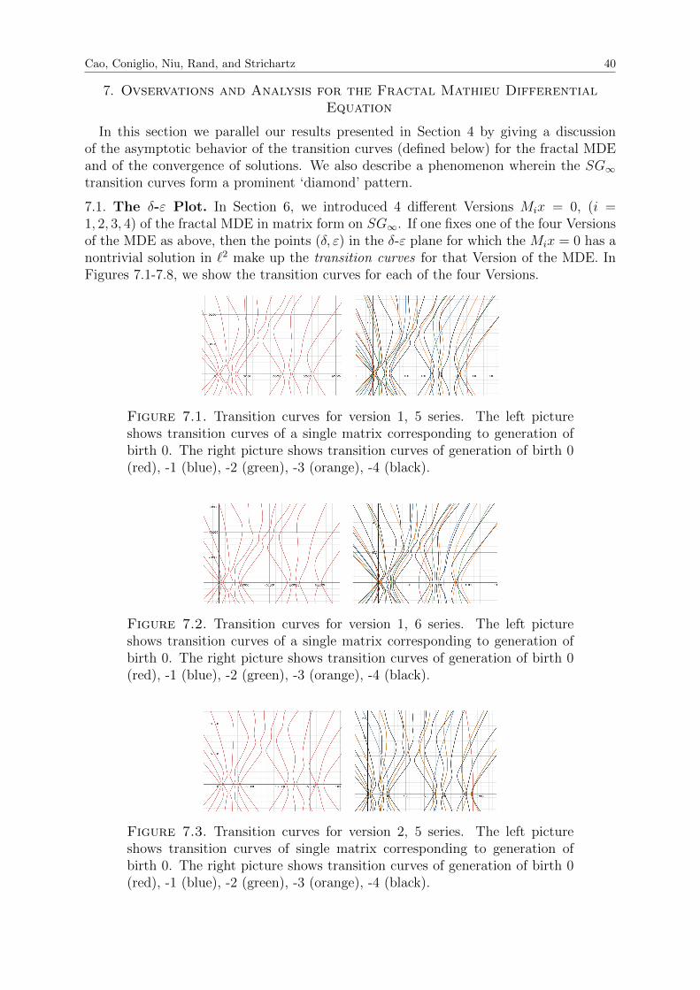
Cao, Coniglio, Niu, Rand, and Strichartz 40
7. Ovservations and Analysis for the Fractal Mathieu DifferentialEquation
In this section we parallel our results presented in Section 4 by giving a discussionof the asymptotic behavior of the transition curves (defined below) for the fractal MDEand of the convergence of solutions. We also describe a phenomenon wherein the SG∞transition curves form a prominent ‘diamond’ pattern.
7.1. The δ-ε Plot. In Section 6, we introduced 4 different Versions Mix = 0, (i =1, 2, 3, 4) of the fractal MDE in matrix form on SG∞. If one fixes one of the four Versionsof the MDE as above, then the points (δ, ε) in the δ-ε plane for which the Mix = 0 has anontrivial solution in `2 make up the transition curves for that Version of the MDE. InFigures 7.1-7.8, we show the transition curves for each of the four Versions.
Figure 7.1. Transition curves for version 1, 5 series. The left pictureshows transition curves of a single matrix corresponding to generation ofbirth 0. The right picture shows transition curves of generation of birth 0(red), -1 (blue), -2 (green), -3 (orange), -4 (black).
Figure 7.2. Transition curves for version 1, 6 series. The left pictureshows transition curves of a single matrix corresponding to generation ofbirth 0. The right picture shows transition curves of generation of birth 0(red), -1 (blue), -2 (green), -3 (orange), -4 (black).
Figure 7.3. Transition curves for version 2, 5 series. The left pictureshows transition curves of single matrix corresponding to generation ofbirth 0. The right picture shows transition curves of generation of birth 0(red), -1 (blue), -2 (green), -3 (orange), -4 (black).

Cao, Coniglio, Niu, Rand, and Strichartz 41
Figure 7.4. Transition curves for version 2, 6 series. The left pictureshows transition curves of single matrix corresponding to generation ofbirth 0. The right picture shows transition curves of generation of birth 0(red), -1 (blue), -2 (green), -3 (orange), -4 (black).
Figure 7.5. Transition curves for version 3, 5 series. The left pictureshows transition curves of single matrix corresponding to generation ofbirth 0. The right picture shows transition curves of generation of birth 0(red), -1 (blue), -2 (green), -3 (orange), -4 (black).
Figure 7.6. Transition curves for version 3, 6 series. The left pictureshows transition curves of single matrix corresponding to generation ofbirth 0. The right picture shows transition curves of generation of birth 0(red), -1 (blue), -2 (green), -3 (orange), -4 (black).
Figure 7.7. Transition curves for version 4, 5 series. The left pictureshows transition curves of single matrix corresponding to generation ofbirth 0. The right picture shows transition curves of generation of birth 0(red), -1 (blue), -2 (green), -3 (orange), -4 (black).

Cao, Coniglio, Niu, Rand, and Strichartz 42
Figure 7.8. Transition curves for version 4, 6 series. The left pictureshows transition curves of single matrix corresponding to generation ofbirth 0. The right picture shows transition curves of generation of birth 0(red), -1 (blue), -2 (green), -3 (orange), -4 (black).
As can be viewed from Figures 7.1-7.8, in each plot there is a ‘diamond’ pattern formedbetween adjacent transition curves. That is, the curves seem to ‘bounce’ off each otherbefore parting in separate directions. This pattern does not appear in the transitioncurves for the Mathieu differential equation on the line. This is one way in which thetransition curves for SG∞ are different than those for the line.
We give a short proof here concerning the asymptotic behavior of the transition curvesfor Versions 1 and 2.
Proposition 7.1. For version 1 and version 2, fix one transition curve. The ratio δε
converges to −1 if ε→∞. The ratio δε
converge to 1 if ε→ −∞.
Proof. In fact, M1 and M2 are of the form A+ ε ·B, where A is a diagonal matrix, andB has one of the following two forms,
B =
0 1
212
0 12
12
0 12
. . . . . .
, or B =
0 1
2
1 0 12
12
0 12
. . . . . .
.The first matrix is real symmetric with continuous spectrum [−1, 1]. To see this, weonly need observe that B = U · cos t · U−1, where U : `2 → L2([0, π]) is defined asUc =
∑∞n=1 cn sinnt. The second one is not symmetric, but we can study the matrix
κ−1(A − εB)κ = A − κ−1Bκ where κ is a diagonal matrix, we did in the proof fortheorem 4. After the transformation, we have
κ−1Bκ =
0 1√
21√2
0 12
12
0 12
. . . . . .
,which is also a real symmetric matrix with continuous spectrum [−1, 1]. Without loss ofgenerality, we just assume B is symmetric in the follows.
In the following proof, we only consider ε → +∞ case, and the other half is thenimmediate by symmetry.
On the k-th curve, we know that
δ = infMk
supc∈Mk
cT (A+ εB)c
cTc,

Cao, Coniglio, Niu, Rand, and Strichartz 43
where the infimum takes over all the k dimensional subspace Mk of domA. It is easy tosee the following lower bound of δ
δ ≥ infMk
supx∈Mk
cTAc
cTc+ inf
Mk
supc∈Mk
εcTBc
cTc= inf
Mk
supx∈Mk
cTAc
cTc− |ε|.
Next, we give an upper bound. For any l < 1, we can find a k dimensional subspaceNk ⊂ domA, such that −1 < B|Nk
< l, which means
−1 <cTBc
cTc< l,∀c ∈ Nk.
In fact, observe that B has continuous spectrum [−1, 1], we can always find a k dimen-sional subspace Nk ⊂ `2 such that −1 < B|Nk
< l. But Nk is not necessarily in domA. Sowe pick a large L, and define
Nk = {c = (c1, c2, · · · , cL, 0, 0, · · ·) : There exists c ∈ Nk such that cj = cj,∀1 ≤ j ≤ L}.
Obviously, Nk ⊂ domA, and −1 < B|Nk< l as long as L is large enough.
Then we get the following upper bound
δ ≤ supc∈Nk
cTAc
cTc+ sup
c∈Nk
εcTBc
cTc< sup
c∈Nk
cTAc
cTc+ lε, for ε > 0.
Combining the upper and lower bounds of δ, we get
−1 ≤ lim infε→+∞
δ
ε≤ lim sup
ε→+∞
δ
ε≤ l.
for any l < 1. Thus limε→+∞δε
= −1. By symmetry, we also get limε→−∞δε
= 1. �
7.2. Solutions of the Mathieu Differential Equation. Now we investigate solutionsto the fractal MDE.
From Corollary 3.3 we deduce that, for ε 6= 0, a nontrivial solution c = (c1, c2, ...) ∈ `2
(or c = (c0, c1, c2, ...) ∈ `2) to any of the four systems Mix = 0 (i = 1, 2, 3, 4) in section
6.2 will decay with asymptotic behaviorcjcj−1∼ βj−1ε
λj−δ . Hence, a solution
u(x) =∞∑j=0
cjϕj(x)
to any of the four versions of the fractal MDE may be well-approximated by the sum ofjust the first few terms in the series, and such an approximation will yield only a smallerror to the actual infinite-series solution.
Recall that in Section 4 we investigated, for the MDE on the line, how properties ofsolutions change if one fixes a transition curve and considers periodic solutions corre-sponding to various (δ, ε) points along that transition curve. We will consider the samequestion for the SG∞ transition curves for the fractal MDE as well.
We investigate this question by first studying the solutions plotted in Figures 7.10-7.29. In constructing the solutions we choose eigenfunctions of generation of birth 2 andof initial eigenvalue 5 or 6, arising from either of the initial functions shown in Figure 7.9,Figures 7.10-7.15 correspond to solutions of Version 1, Figures 7.16-7.21 correspond to

Cao, Coniglio, Niu, Rand, and Strichartz 44
solutions of Version 2, Figures 7.22-7.25 correspond to solutions of Version 3, and Figures7.26-7.29 correspond to solutions of Version 4. Each Figure includes two images. Theone on the left is a plot of three different solutions corresponding to different (δ, ε) pairsalong the first transition curve; the set of three solutions in each Figure corresponds toeither 5-series or 6-series, and each solution been normalized so that the maximum valueit attains is 1. The image on the right in each Figure shows an overlook of the threesolutions, where the color at each point indicates which solution takes on the biggestvalue among the three. From the plots, it is evident that these normalized solutions seemto converge as ε tends to infinity along the first transition curve.
The second way in which we investigate the question is by observing the behavior of thelocation of relative maxima of solutions as ε traverses along a transition curve. Here westill choose to study (δ, ε) pairs and corresponding solutions on the first transition curvefor each version. See Figure 7.30-7.37. This is analogous to our study of the relativemaxima of solutions to the MDE on the line in Section 4.2. Each of the Figures containstwo images indicating the position of relative maxima: the image on the left shows howthe positions of the maximas move as ε becomes larger, and the image on the right is anoverlook of the left one where we can clearly see the locations of the peaks. We makeseveral observations:
• The first thing we can see is that the movement of the peaks are not large, andwe do not observe the peaks converging to the boundary.
• The second observation is that the 5 and 6 series behave quite differently. Wecan observe jumps of peaks in all the versions for 5 series, but the number ofpeaks is usually 3. A special case is figure 7.36, where many peaks occur when εis quite large. However, for 6 series, we can observe many more peaks when ε isvery small, but most of them do not appear when ε is large. Until now, we donot have explanation for these behaviors.
1 −1
1
−1 1
−1
11
1
−1 −1
−1
Figure 7.9. Initial values of the eigenfunctions with birth of generation2 and initial eigenvalues 5 (left) and 6(right).

Cao, Coniglio, Niu, Rand, and Strichartz 45
Figure 7.10. Solutions on the first curve for choice 1, initial eigenvalue5, with ε = 1000, 2000, 3000.
Figure 7.11. Solutions on the first curve for choice 1, initial eigenvalue5, with ε = 10000, 11000, 12000.
Figure 7.12. Solutions on the first curve for choice 1, initial eigenvalue5, with ε = 20000, 25000, 30000.

Cao, Coniglio, Niu, Rand, and Strichartz 46
Figure 7.13. Solutions on the first curve for choice 1, initial eigenvalue6, initial eigenvalue 6, with ε = 1000, 2000, 3000.
Figure 7.14. Solutions on the first curve for choice 1, initial eigenvalue6, initial eigenvalue 6, with, with ε = 10000, 11000, 12000.
Figure 7.15. Solutions on the first curve for choice 1, initial eigenvalue6, initial eigenvalue 6, with ε = 20000, 25000, 30000.
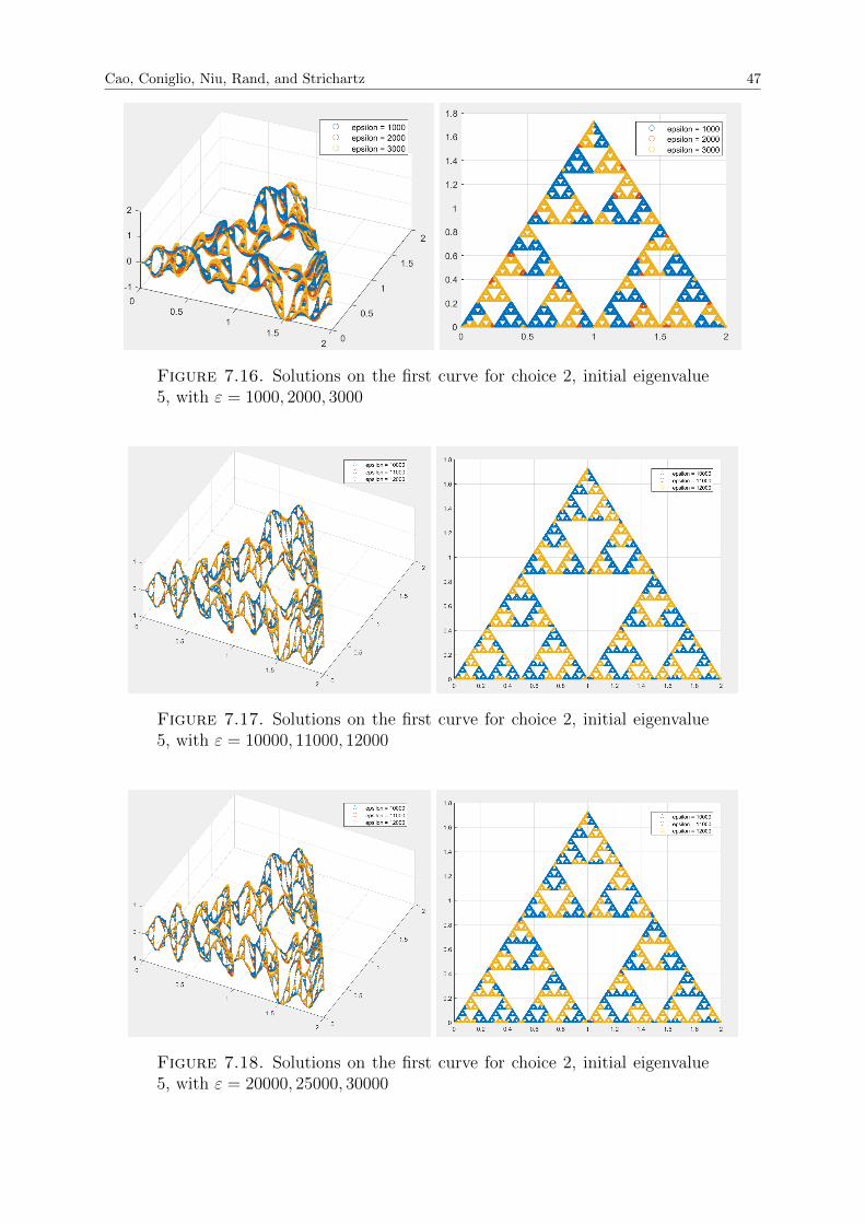
Cao, Coniglio, Niu, Rand, and Strichartz 47
Figure 7.16. Solutions on the first curve for choice 2, initial eigenvalue5, with ε = 1000, 2000, 3000
Figure 7.17. Solutions on the first curve for choice 2, initial eigenvalue5, with ε = 10000, 11000, 12000
Figure 7.18. Solutions on the first curve for choice 2, initial eigenvalue5, with ε = 20000, 25000, 30000

Cao, Coniglio, Niu, Rand, and Strichartz 48
Figure 7.19. Solutions on the first curve for choice 2, initial eigenvalue6, with ε = 1000, 2000, 3000.
Figure 7.20. Solutions on the first curve for choice 2, initial eigenvalue6, initial eigenvalue 6, with, with ε = 10000, 11000, 12000.
Figure 7.21. Solutions on the first curve for choice 2, initial eigenvalue6, initial eigenvalue 6, with ε = 20000, 25000, 30000.

Cao, Coniglio, Niu, Rand, and Strichartz 49
Figure 7.22. Solutions on the first curve for choice 3, initial eigenvalue5, with ε = 1000, 2000, 3000.
Figure 7.23. Solutions on the first curve for choice 3, initial eigenvalue5, with ε = 20000, 25000, 30000.
Figure 7.24. Solutions on the first curve for choice 3, initial eigenvalue6, with ε = 1000, 2000, 3000.

Cao, Coniglio, Niu, Rand, and Strichartz 50
Figure 7.25. Solutions on the first curve for choice 3, initial eigenvalue6, with ε = 20000, 25000, 30000.
Figure 7.26. Solutions on the first curve for choice 4, initial eigenvalue5, with ε = 1000, 2000, 3000.
Figure 7.27. Solutions on the first curve for choice 4, initial eigenvalue5, with ε = 20000, 25000, 30000.

Cao, Coniglio, Niu, Rand, and Strichartz 51
Figure 7.28. Solutions on the first curve for choice 4, initial eigenvalue6, with ε = 1000, 2000, 3000.
Figure 7.29. Solutions on the first curve for choice 4, initial eigenvalue6, with ε = 20000, 25000, 30000.

Cao, Coniglio, Niu, Rand, and Strichartz 52
Figure 7.30. The position of peaks for version 1, 5 series.
Figure 7.31. The position of peaks for version 1, 6 series.
Figure 7.32. The position of peaks for version 2, 5 series.

Cao, Coniglio, Niu, Rand, and Strichartz 53
Figure 7.33. The position of peaks for version 2, 6 series.
-
Figure 7.34. The position of peaks for version 3, 5 series.
Figure 7.35. The position of peaks for version 3, 6 series.

Cao, Coniglio, Niu, Rand, and Strichartz 54
-
Figure 7.36. The position of peaks for version 4, 5 series.
Figure 7.37. The position of peaks for version 4, 6 series.
8. Further Research
Now we discuss further research questions that can be investigated in this area.
(i) Asymptotic behavior of SG∞ transition curves
One could further investigate the asymptotic behavior of the SG∞ transitioncurves. For the line case, we have Theorem 4.2 due to W.S. Loud, stating that
δ = −ε+
(k − 1
2
)√2ε+O(ε1/2)
as ε→ +∞ on the k−th transition curve. We can investigate whether estimatesof a similar form hold on SG∞. This would include extending Proposition 7.1 toVersion 3 and Version 4 the MDE on SG∞.
(ii) Other modifications of MDE matrix
Further research could investigate different matrix versions of the fractal MDE,aside from Versions 1-4 presented in Section 6.
Cao, Coniglio, Niu, Rand, and Strichartz 55
(iii) Other Fractal Domains
One could investigate how the Mathieu differential equation could be extendedto other infinite fractafolds. Such infinite fractafolds may or may not be basedon SG.
(iv) The Hill Equation
The Mathieu differential equation is actually a special case of the so-called Hilldifferential equation. The Hill differential equation is given by
d2u
dt2+ f(t)u = 0,
where f(t) is an arbitrary periodic function. Readers can read [21, 16, 17, 28] fordetails. Further research could investigate ways in which to extend, for variouschoices of f(x), the Hill differential equation to be defined on fractal domains.
9. Appendix
In this appendix we derive equations in matrix form for solutions to the MDE on theline which have period 2Nπ, N ∈ N. We will use a similar procedure as in Section 2 andwill obtain tridiagonal matrices.
Let u be a solution with period 2Nπ. We can write the Fourier expansion of u as
u(t) =∞∑j=0
aj cos
(j
Nt
)+∞∑j=1
bj sin
(j
Nt
). (9.1)
Plugging in this Fourier series for u into the Mathieu differential equation, we obtaintwo infinite systems of linear homogeneous equations for the cosine and sine coefficients,respectively, as follows:
cosine coefficients
δa0 + ε
2aN = 0,
(δ − j2)aj + ε2(aN−j + aN+j) = 0 if 1 ≤ j ≤ N − 1,
(δ −N2)aN + ε2(2a0 + a2N) = 0,
(δ − j2)aj + ε2(aj−N + aj+N) = 0 if j ≥ N + 1,
and
sine coefficients
(δ − j2)bj + ε
2(bN+j − bN−j) = 0 if 1 ≤ j ≤ N − 1,
(δ −N2)bN + ε2b2N = 0,
(δ − j2)bj + ε2(bj−N + bj+N) = 0 if j ≥ N + 1.
We can immediately write the equations in the matrix form, but the result is unwieldy.So, we make further classifications of the coefficients, just as we did in Section 2.2, wherecoefficients are separated into two classes—those with even indices and those with andodd indexes.
A natural criterion is to have coefficients that appear in the same equation be in asame class. For example, a0 and aN should be in a same class. Based on this idea, wesay that aj and aj′ (or bj and bj′) are in the ‘same class’ if and only if there is a finitesequence
aj = aj0 , aj1 , aj2 , · · · , ajL = aj′ ,

Cao, Coniglio, Niu, Rand, and Strichartz 56
such that ajl and ajl+1appear in a same equation for all 0 ≤ l ≤ L − 1. For example,
a0 and a3N are in the same class, since we a0 and aN are in the same equation, aN anda2N are in the same equation, and a2N and a3N are in the same equation. It is easy tocheck that the the property of being in the ‘same class’ is an equivalence relation on theset {aj : j ≥ 0} and on the set {bj : j ≥ 1}. This partitions {aj : j ≥ 0} into [N
2] + 1
different equivalence classes and partitions {bj : j ≥ 0} into [N2
] + 1 different equivalenceclasses. So we can write equations for different equivalence classes separately. Below, wediscuss all the possible cases. First we give a discussion for the cosine coefficients {aj}.As we will see, the case for the sine coefficients {bj} is similar.
There are three possible forms that the matrix corresponding to any particular equiv-alence class can take:
1). The first possible equivalence class is {a0, aN , a2N , · · ·}, with the correspondingmatrix equation
δ ε
2
ε δ − 1 ε2
ε2
δ − 22 ε2
. . . . . . . . .
a0
aNa2N
...
...
=
000......
.
Note that this is just the equation Ax = 0 in Section 2.2. If there is a nontriv-ial solution to the above equation, then the MDE has a 2π periodic solution, sinceu(t) =
∑∞l=0 alN cos(lt) solves the MDE.
2). The second form that an equivalence class can take is
{a|k−lN |}∞l=−∞ = {ak, ak+N , ak2N ,···} ∪ {aN−k, a2N−k, · · ·},
where 1 ≤ k < N2
. The corresponding equations can be written in the form
. . . . . . . . .
δ −(
2N−kN
)2 ε2
ε2
δ −(N−kN
)2 ε2
ε2
δ −(kN
)2 ε2
ε2
δ −(N+kN
)2 ε2
. . . . . . . . .
...a2N−kaN−kakak+N
...
=
...00000...
.
If there is a nontrivial solution to the above equation, then u(t) =∑∞
l=−∞ ak+lN cos(k+lNN
t)
is a 2Nπ
gcd(N,K)-periodic solution to the MDE, where gcd(N, k) denotes the greatest common
divisor of the pair (N, k).In particular, we get a 2Nπ-periodic solution to the MDE from the equation above if
and only if k and N are coprime. Thus, the matrices of the second form with k and Ncoprime yield 2Nπ-periodic solutions.
3) The third form that an equivalence class can take is {aN2, a 3
2N , a 5
2N , · · ·}. This form
can only occur if N is even. The corresponding equations can be written in the form

Cao, Coniglio, Niu, Rand, and Strichartz 57
δ − 1
4+ ε
2ε2
ε2
δ − 32
4ε2
ε2
δ − 52
4ε2
. . . . . . . . .
aN2
a 3N2
a 5N2......
=
000......
.
The above matrix is exactly the matrix C in Section 2.2, which yield 4π-periodic solutions.
The matrix forms for sine coefficients are quite similar to those for the cosine coeffi-cients. For solutions of period 2Nπ,N ≥ 3, the equations for sine coefficents have thefollowing form
. . . . . . . . .
δ − (2N−kN
)2 ε2
ε2
δ − (N−kN
)2 − ε2
− ε2
δ − ( kN
)2 ε2
ε2
δ − (N+kN
)2 ε2
. . . . . . . . .
...b2N−kbN−kbkbk+N
...
=
...00000...
,
where k can by any integer such that k and N are coprime.
References
[1] N. Asai, D. Cai, Y. Ikebe, and Y. Miyazaki. “The Eigenvalue Problem for InfiniteComplex Symmetric Tridiagonal Matrices With Application”. In: Linear AlgebraAppl. 241 (1996), pp. 599–618.
[2] J. Avron and B. Simon. “The asymptotics of the gap in the Mathieu equation”. In:Ann. Physics 134 (1981), pp. 76–84.
[3] O. Ben-Bassat, R.S. Strichartz, and A. Teplyaev. “What Is Not in the Domain ofthe Laplacian on Sierpinski Gasket Type Fractals”. In: J. Funct. Anal. 166 (1999),pp. 197–217.
[4] S. Cao, A. Coniglio, X. Niu, R. Rand, and R.S. Strichartz. The Mathieu DifferentialEquation and Generalizations to Infinite Fractafolds. 2019. url: http://pi.math.cornell.edu/∼aac254.
[5] K. Dalrymple, R.S. Strichartz, and J.P. Vinson. “Fratal Differential Equations onthe Sierpinski Gasket”. In: J. Fourier Anal. Appl. 5 (1999), pp. 203–284.
[6] S. Du, Y. Jia, and A. A. Seshia. “Twenty-Eight Orders of Parametric Resonance ina Microelectromechanical Device for Multi-band Vibration Energy Harvesting”. In:Sci. Rep. 6 (2016), p. 30167.
[7] K. Falconer. Fractal Geometry. John Wiley & Sons, 2014.
[8] M. Fukushima and T. Shima. “On a spectral analysis for the Sierpinski gasket”. In:Potential Anal. 1 (1992), pp. 1–35.
[9] A. Gil, S. Javier, and N. M. Temme. Numerical methods for special functions.Vol. 99. Society for Industrial and Applied Mathematics, 2007.
Cao, Coniglio, Niu, Rand, and Strichartz 58
[10] H. Hochstadt. “On the Width of the Instability Intervals of the Mathieu Equation”.In: SIAM J. Math. Anal. 15.1 (1984), pp. 105–107.
[11] J.E. Hutchinson. “Fractals and self-similarity”. In: Indiana Univ. Math. J. 30 (1981),pp. 713–747.
[12] M. Ionescu, L.G. Rogers, and R.S. Strichartz. “Pseudo-differential operators on frac-tals and other metric measure spaces”. In: Rev. Mat. Iberoam. 29 (2013), pp. 1159–1190.
[13] J. Kigami. “A harmonic calculus on the Sierpinski spaces”. In: Japan J. Appl. Math.6.2 (1989), pp. 259–290.
[14] J. Kigami. Analysis on fractals. Vol. 143. Cambridge Tracts in Mathematics. Cam-bridge University Press, Cambridge, 2001.
[15] J. Kigami. “Harmonic calculus on p.c.f. self-similar sets”. In: Trans. Amer. Math.Soc. 335.2 (1993), pp. 721–755.
[16] D. M. Levy and J. B. Keller. “Instability Intervals of Hill’s Equation”. In: Comm.Pure Appl. Math. 16.4 (1963), pp. 469–476.
[17] W. S. Loud. “Stability regions for Hill’s equation”. In: J. Differential Equations 19(1975), pp. 226–241.
[18] R. H. Rand. Mathieu’s Equation. International Centre for Mechanical Sciences,2016.
[19] R.H. Rand. Computer Algebra in Applied Mathematics: An Introduction to MAC-SYMA. Vol. 94. Pitman Advanced Publishing Program, 1984.
[20] H. Ruan and R.S. Strichartz. “Covering maps and periodic functions on higherdimensional Sierpinski gaskets”. In: Canad. J. Math. 61.5 (2009), pp. 1151–1181.
[21] J. J. Stoker. Nonlinear vibrations in mechanical and electrical systems. Vol. 2. NewYork: Interscience Publishers, 1950.
[22] R.S. Strichartz. Differential Equations on Fractals: A Tutorial. Princeton UniversityPress, 2006.
[23] R.S. Strichartz. “Fractafolds based on the Sierpinski gasket and their spectra”. In:Trans. Amer. Math. Soc. 355.10 (2003), pp. 4019–4043.
[24] R.S. Strichartz. “Fractals in the large”. In: Can. J. Math. 50 (1996), pp. 638–657.
[25] R.S. Strichartz. “Periodic and almost periodic functions on infinite Sierpinski gas-kets”. In: Canad. J. Math. 61.5 (2009), pp. 1182–1200.
[26] R.S. Strichartz and A. Teplyaev. “Spectral analysis on infinite Sierpinski fractafolds”.In: J. Anal. Math. 116 (2012), pp. 255–297.
[27] A. Teplyaev. “Spectral Analysis on Infinite Sierpinski Gaskets”. In: J. Funct. Anal.159.2 (1998), pp. 537–567.
[28] M. I. Weinstein and J. B. Keller. “Asymptotic Behavior of Stability Regions forHill’s Equation”. In: J. Appl. Math. 47.5 (1987), pp. 941–958.