The mathematics of REML - StATS
91
The mathematics of REML A workshop conducted at Universitas Brawijaya, Malang, Indonesia December 2013 Mick O'Neill Statistical Advisory & Training Service Pty Ltd [email protected] www.stats.net.au
Transcript of The mathematics of REML - StATS
The mathematics of REML
A workshop conducted at
Universitas Brawijaya, Malang, Indonesia
December 2013
Mick O'Neill
Statistical Advisory & Training Service Pty Ltd
www.stats.net.au
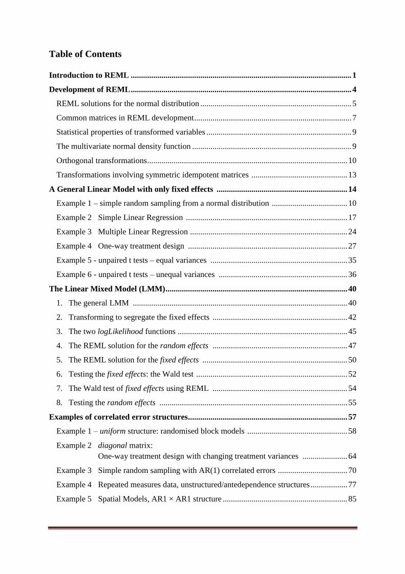
Table of Contents
Introduction to REML ............................................................................................................ 1
Development of REML ............................................................................................................ 4
REML solutions for the normal distribution .......................................................................... 5
Common matrices in REML development ............................................................................. 7
Statistical properties of transformed variables ....................................................................... 9
The multivariate normal density function .............................................................................. 9
Orthogonal transformations .................................................................................................. 10
Transformations involving symmetric idempotent matrices ............................................... 13
A General Linear Model with only fixed effects ................................................................ 14
Example 1 – simple random sampling from a normal distribution ..................................... 10
Example 2 Simple Linear Regression ............................................................................... 17
Example 3 Multiple Linear Regression ............................................................................. 24
Example 4 One-way treatment design .............................................................................. 27
Example 5 - unpaired t tests – equal variances ................................................................... 35
Example 6 - unpaired t tests – unequal variances ............................................................... 36
The Linear Mixed Model (LMM) ......................................................................................... 40
1. The general LMM ......................................................................................................... 40
2. Transforming to segregate the fixed effects .................................................................. 42
3. The two logLikelihood functions ................................................................................... 45
4. The REML solution for the random effects .................................................................. 47
5. The REML solution for the fixed effects ....................................................................... 50
6. Testing the fixed effects: the Wald test .......................................................................... 52
7. The Wald test of fixed effects using REML .................................................................. 54
8. Testing the random effects ............................................................................................ 55
Examples of correlated error structures.............................................................................. 57
Example 1 – uniform structure: randomised block models ................................................. 58
Example 2 diagonal matrix:
One-way treatment design with changing treatment variances ...................... 64
Example 3 Simple random sampling with AR(1) correlated errors .................................. 70
Example 4 Repeated measures data, unstructured/antedependence structures .................. 77
Example 5 Spatial Models, AR1 × AR1 structure ............................................................. 85
The Mathematics of REML
1
An introduction to REML
REML stands for
REsidual Maximum Likelihood
or sometimes
REstricted Maximum Likelihood
or even
REduced Maximum Likelihood (Patterson and Thompson, 1971)
So what is Maximum Likelihood?
The likelihood of a sample is the prior probability of obtaining the data in your sample.
This requires you to assume that the data follow some distribution, typically
Binomial or Poisson for count data
Normal or LogNormal for continuous data
Each of these distributions involves at least one unknown parameter which must be
estimated from the data.
Estimation is often achieved by finding that value of the parameter which maximises the
likelihood.
This value is referred to as the maximum likelihood estimate of the parameter.
Note.
It turns out that maximising the log-likelihood is equivalent to maximising the likelihood and
is easier to deal with (for numeric accuracy).
The Mathematics of REML
2
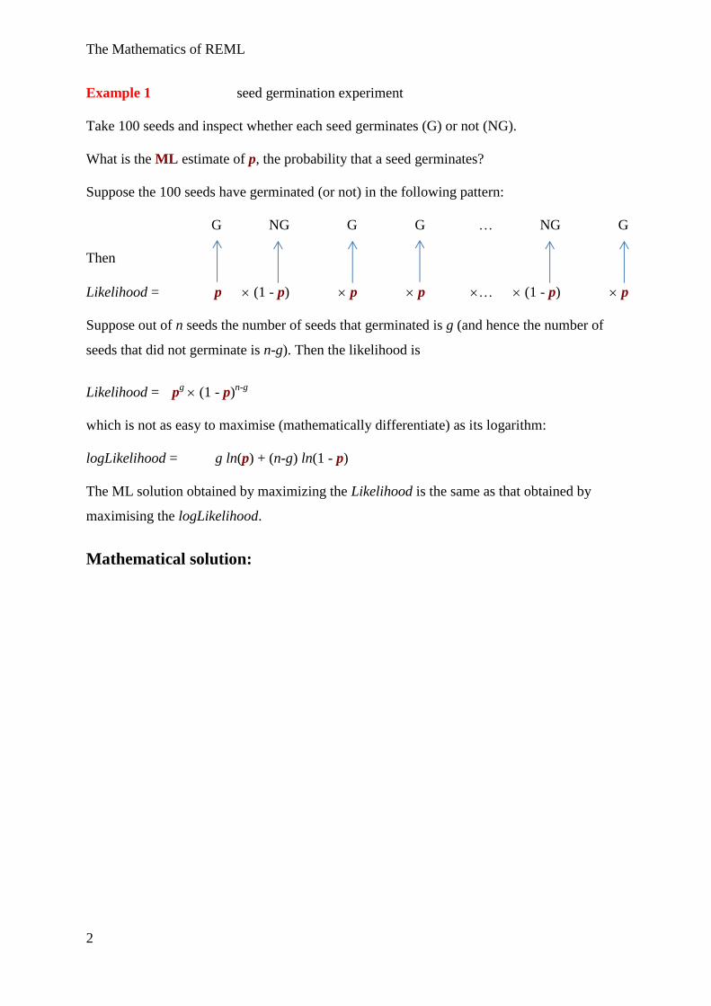
Example 1 seed germination experiment
Take 100 seeds and inspect whether each seed germinates (G) or not (NG).
What is the ML estimate of p, the probability that a seed germinates?
Suppose the 100 seeds have germinated (or not) in the following pattern:
G NG G G … NG G
Then
Likelihood = p (1 - p) p p … (1 - p) p
Suppose out of n seeds the number of seeds that germinated is g (and hence the number of
seeds that did not germinate is n-g). Then the likelihood is
Likelihood = pg (1 - p)
n-g
which is not as easy to maximise (mathematically differentiate) as its logarithm:
logLikelihood = g ln(p) + (n-g) ln(1 - p)
The ML solution obtained by maximizing the Likelihood is the same as that obtained by
maximising the logLikelihood.
Mathematical solution:
The Mathematics of REML
3
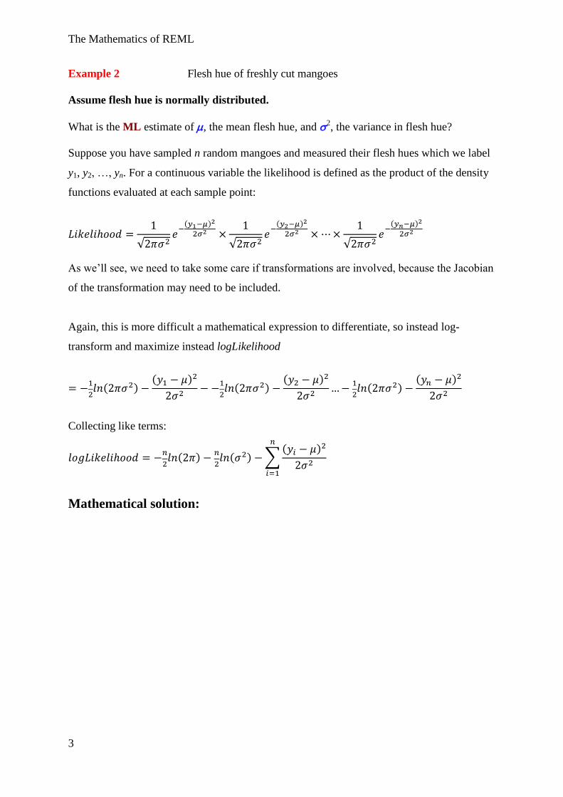
Example 2 Flesh hue of freshly cut mangoes
Assume flesh hue is normally distributed.
What is the ML estimate of , the mean flesh hue, and 2, the variance in flesh hue?
Suppose you have sampled n random mangoes and measured their flesh hues which we label
y1, y2, …, yn. For a continuous variable the likelihood is defined as the product of the density
functions evaluated at each sample point:
√
( )
√
( )
√
( )
As we’ll see, we need to take some care if transformations are involved, because the Jacobian
of the transformation may need to be included.
Again, this is more difficult a mathematical expression to differentiate, so instead log-
transform and maximize instead logLikelihood
( )
( )
( )
( )
( )
( )
Collecting like terms:
( )
( ) ∑
( )
Mathematical solution:
The Mathematics of REML
4
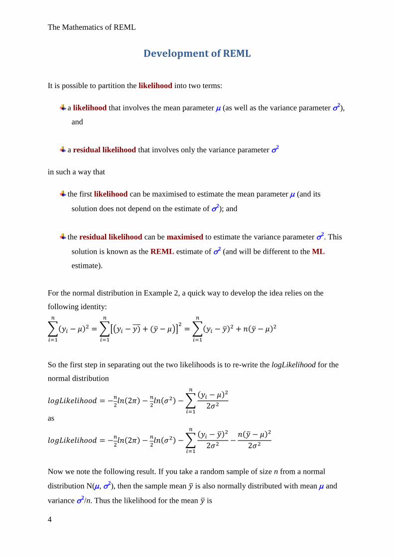
Development of REML
It is possible to partition the likelihood into two terms:
a likelihood that involves the mean parameter (as well as the variance parameter 2),
and
a residual likelihood that involves only the variance parameter 2
in such a way that
the first likelihood can be maximised to estimate the mean parameter (and its
solution does not depend on the estimate of 2); and
the residual likelihood can be maximised to estimate the variance parameter 2. This
solution is known as the REML estimate of 2 (and will be different to the ML
estimate).
For the normal distribution in Example 2, a quick way to develop the idea relies on the
following identity:
∑( )
∑[( ) ( )]
∑( )
( )
So the first step in separating out the two likelihoods is to re-write the logLikelihood for the
normal distribution
( )
( ) ∑
( )
as
( )
( ) ∑
( )
( )
Now we note the following result. If you take a random sample of size n from a normal
distribution N(, 2), then the sample mean is also normally distributed with mean and
variance 2/n. Thus the likelihood for the mean is
The Mathematics of REML
5
√ ⁄
( )
⁄ √
( )
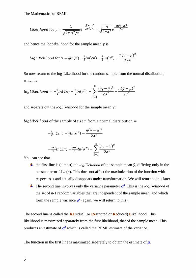
and hence the logLikelihood for the sample mean is
( )
( )
( )
( )
So now return to the log-Likelihood for the random sample from the normal distribution,
which is
( )
( ) ∑
( )
( )
and separate out the logLikelihood for the sample mean :
( )
( )
( )
( )
( ) ∑
( )
You can see that
the first line is (almost) the loglikelihood of the sample mean , differing only in the
constant term -½ ln(n). This does not affect the maximization of the function with
respect to and actually disappears under transformation. We will return to this later.
The second line involves only the variance parameter 2. This is the loglikelihood of
the set of n-1 random variables that are independent of the sample mean, and which
form the sample variance 2 (again, we will return to this).
The second line is called the REsidual (or Restricted or Reduced) Likelihood. This
likelihood is maximized separately from the first likelihood, that of the sample mean. This
produces an estimate of 2 which is called the REML estimate of the variance.
The function in the first line is maximized separately to obtain the estimate of .
The Mathematics of REML
6
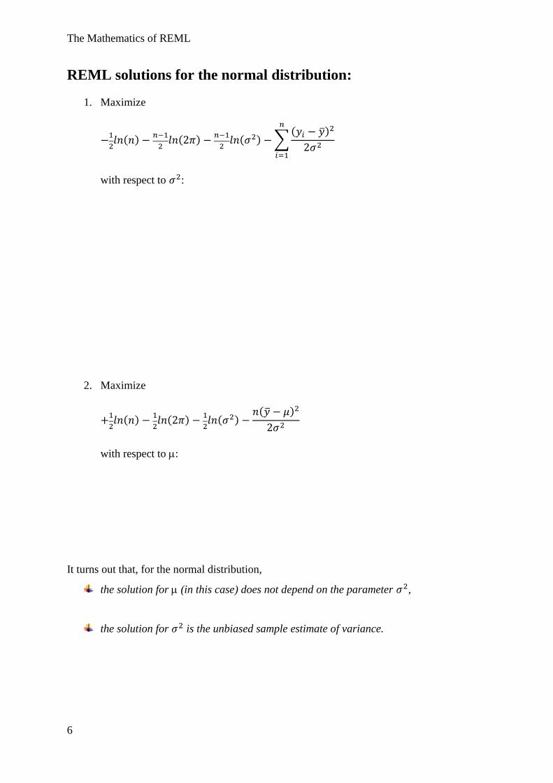
REML solutions for the normal distribution:
1. Maximize
( )
( )
( ) ∑
( )
with respect to :
2. Maximize
( )
( )
( )
( )
with respect to :
It turns out that, for the normal distribution,
the solution for (in this case) does not depend on the parameter ,
the solution for is the unbiased sample estimate of variance.
The Mathematics of REML
7
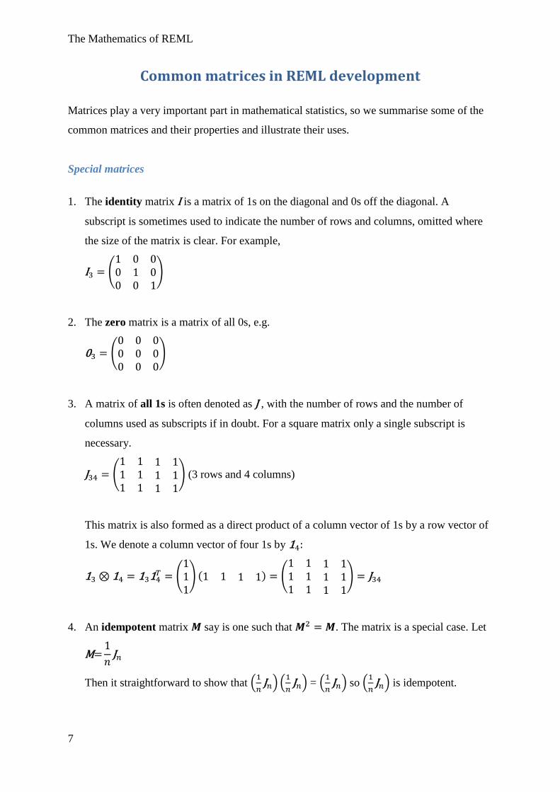
Common matrices in REML development
Matrices play a very important part in mathematical statistics, so we summarise some of the
common matrices and their properties and illustrate their uses.
Special matrices
1. The identity matrix is a matrix of 1s on the diagonal and 0s off the diagonal. A
subscript is sometimes used to indicate the number of rows and columns, omitted where
the size of the matrix is clear. For example,
(
)
2. The zero matrix is a matrix of all 0s, e.g.
(
)
3. A matrix of all 1s is often denoted as , with the number of rows and the number of
columns used as subscripts if in doubt. For a square matrix only a single subscript is
necessary.
(
) (3 rows and 4 columns)
This matrix is also formed as a direct product of a column vector of 1s by a row vector of
1s. We denote a column vector of four 1s by
(
) ( ) (
)
4. An idempotent matrix say is one such that . The matrix is a special case. Let
Then it straightforward to show that (
) (
) = (
) so (
) is idempotent.
The Mathematics of REML
8
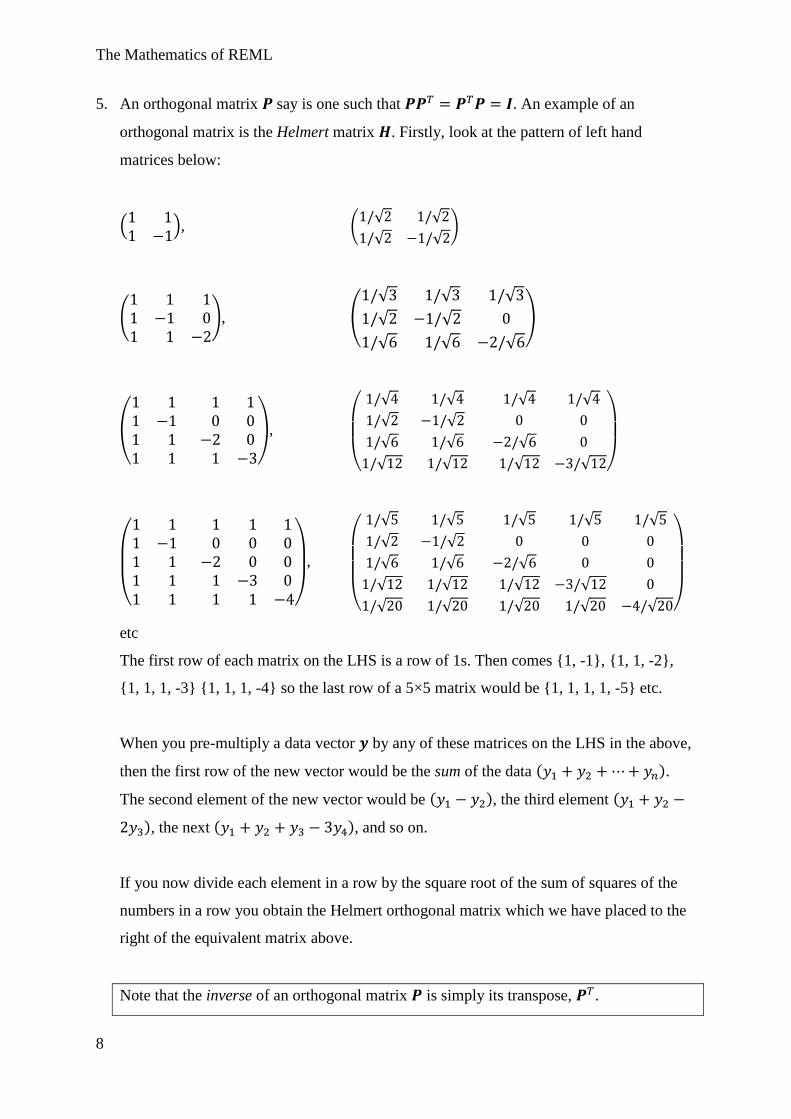
5. An orthogonal matrix say is one such that . An example of an
orthogonal matrix is the Helmert matrix . Firstly, look at the pattern of left hand
matrices below:
(
), ( √ √
√ √ )
(
), (
√ √ √
√ √
√ √ √
)
(
),
(
√ √ √ √
√ √
√ √ √
√ √ √ √ )
(
)
,
(
√ √ √ √ √
√ √
√ √ √
√ √ √ √
√ √ √ √ √ )
etc
The first row of each matrix on the LHS is a row of 1s. Then comes {1, -1}, {1, 1, -2},
{1, 1, 1, -3} {1, 1, 1, -4} so the last row of a 5×5 matrix would be {1, 1, 1, 1, -5} etc.
When you pre-multiply a data vector by any of these matrices on the LHS in the above,
then the first row of the new vector would be the sum of the data ( ).
The second element of the new vector would be ( ), the third element (
), the next ( ), and so on.
If you now divide each element in a row by the square root of the sum of squares of the
numbers in a row you obtain the Helmert orthogonal matrix which we have placed to the
right of the equivalent matrix above.
Note that the inverse of an orthogonal matrix is simply its transpose, .
The Mathematics of REML
9
Statistical properties of transformed variables
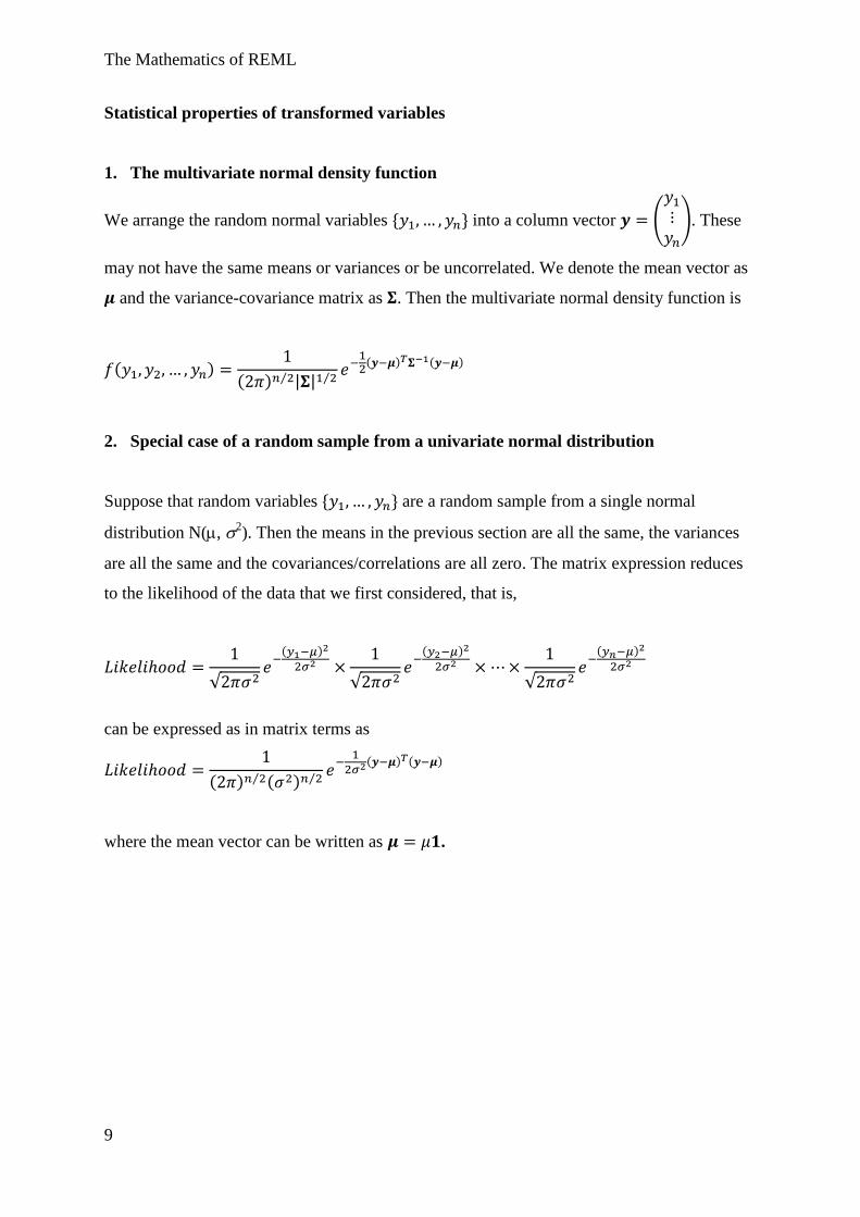
1. The multivariate normal density function
We arrange the random normal variables into a column vector (
). These
may not have the same means or variances or be uncorrelated. We denote the mean vector as
and the variance-covariance matrix as . Then the multivariate normal density function is
( )
( ) ⁄ | | ⁄
( ) ( )
2. Special case of a random sample from a univariate normal distribution
Suppose that random variables are a random sample from a single normal
distribution N(, 2). Then the means in the previous section are all the same, the variances
are all the same and the covariances/correlations are all zero. The matrix expression reduces
to the likelihood of the data that we first considered, that is,
√
( )
√
( )
√
( )
can be expressed as in matrix terms as
( ) ⁄ ( ) ⁄
( ) ( )
where the mean vector can be written as .
The Mathematics of REML
10
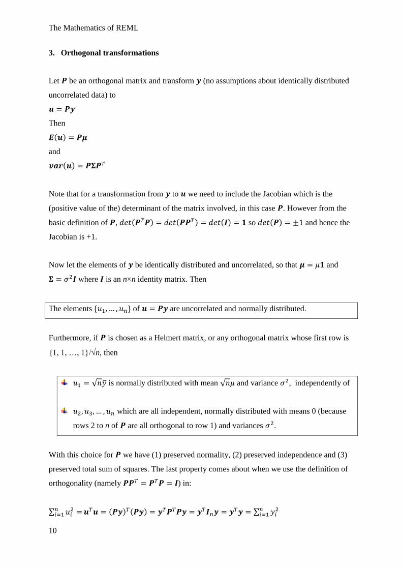
3. Orthogonal transformations
Let be an orthogonal matrix and transform (no assumptions about identically distributed
uncorrelated data) to
Then
( )
and
( )
Note that for a transformation from to we need to include the Jacobian which is the
(positive value of the) determinant of the matrix involved, in this case . However from the
basic definition of , ( ) ( ) ( ) so ( ) and hence the
Jacobian is +1.
Now let the elements of be identically distributed and uncorrelated, so that and
where is an n×n identity matrix. Then
The elements of are uncorrelated and normally distributed.
Furthermore, if is chosen as a Helmert matrix, or any orthogonal matrix whose first row is
{1, 1, …, 1}/n, then
√ is normally distributed with mean √ and variance , independently of
which are all independent, normally distributed with means 0 (because
rows 2 to n of are all orthogonal to row 1) and variances .
With this choice for we have (1) preserved normality, (2) preserved independence and (3)
preserved total sum of squares. The last property comes about when we use the definition of
orthogonality (namely ) in:
∑
( ) ( ) ∑
The Mathematics of REML
11
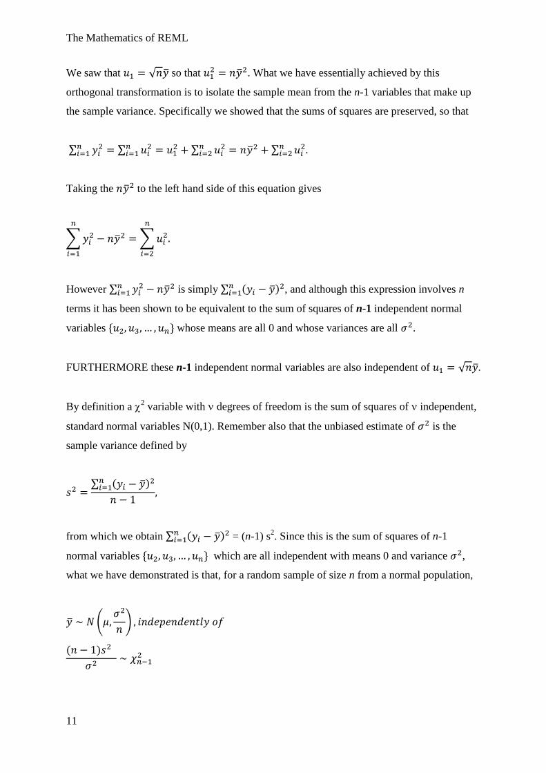
We saw that √ so that . What we have essentially achieved by this
orthogonal transformation is to isolate the sample mean from the n-1 variables that make up
the sample variance. Specifically we showed that the sums of squares are preserved, so that
∑
∑
∑
∑
Taking the to the left hand side of this equation gives
∑
∑
However ∑
is simply ∑ ( ) , and although this expression involves n
terms it has been shown to be equivalent to the sum of squares of n-1 independent normal
variables whose means are all 0 and whose variances are all .
FURTHERMORE these n-1 independent normal variables are also independent of √
By definition a 2 variable with degrees of freedom is the sum of squares of independent,
standard normal variables N(0,1). Remember also that the unbiased estimate of is the
sample variance defined by
∑ ( )
from which we obtain ∑ ( ) = (n-1) s
2. Since this is the sum of squares of n-1
normal variables which are all independent with means 0 and variance ,
what we have demonstrated is that, for a random sample of size n from a normal population,
(
)
( )
The Mathematics of REML
12
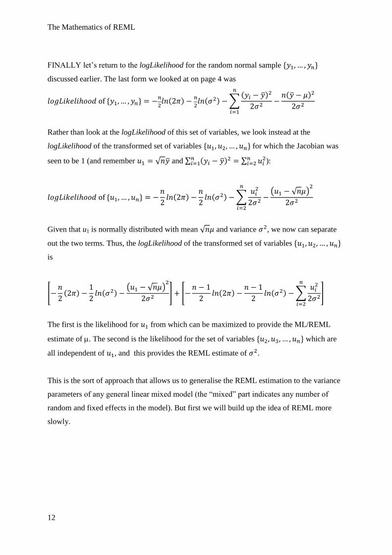
FINALLY let’s return to the logLikelihood for the random normal sample
discussed earlier. The last form we looked at on page 4 was
( )
( ) ∑
( )
( )
Rather than look at the logLikelihood of this set of variables, we look instead at the
logLikelihood of the transformed set of variables for which the Jacobian was
seen to be 1 (and remember √ and ∑ ( ) ∑
):
( )
( ) ∑
( √ )
Given that u1 is normally distributed with mean √ and variance , we now can separate
out the two terms. Thus, the logLikelihood of the transformed set of variables
is
[
( )
( )
( √ )
] [
( )
( ) ∑
]
The first is the likelihood for from which can be maximized to provide the ML/REML
estimate of . The second is the likelihood for the set of variables which are
all independent of , and this provides the REML estimate of .
This is the sort of approach that allows us to generalise the REML estimation to the variance
parameters of any general linear mixed model (the “mixed” part indicates any number of
random and fixed effects in the model). But first we will build up the idea of REML more
slowly.
The Mathematics of REML
13
4. Transformations involving symmetric idempotent matrices
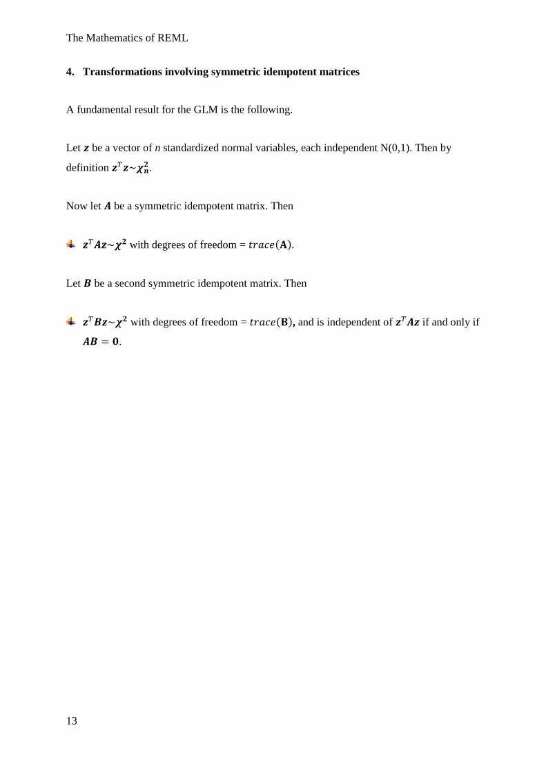
A fundamental result for the GLM is the following.
Let be a vector of n standardized normal variables, each independent N(0,1). Then by
definition .
Now let be a symmetric idempotent matrix. Then
with degrees of freedom = ( ).
Let be a second symmetric idempotent matrix. Then
with degrees of freedom = ( ), and is independent of if and only if
.
The Mathematics of REML
14
A General Linear Model with only fixed effects
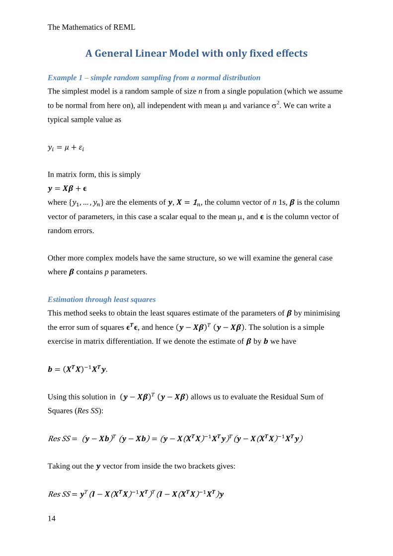
Example 1 – simple random sampling from a normal distribution
The simplest model is a random sample of size n from a single population (which we assume
to be normal from here on), all independent with mean and variance 2. We can write a
typical sample value as
In matrix form, this is simply
where are the elements of , , the column vector of n 1s, is the column
vector of parameters, in this case a scalar equal to the mean , and is the column vector of
random errors.
Other more complex models have the same structure, so we will examine the general case
where contains p parameters.
Estimation through least squares
This method seeks to obtain the least squares estimate of the parameters of by minimising
the error sum of squares , and hence ( ) ( ). The solution is a simple
exercise in matrix differentiation. If we denote the estimate of by we have
( )
Using this solution in ( ) ( ) allows us to evaluate the Residual Sum of
Squares (Res SS):
( ) ( ) ( ( ) ) ( ( ) )
Taking out the vector from inside the two brackets gives:
( ( ) ) ( ( ) )
The Mathematics of REML
15
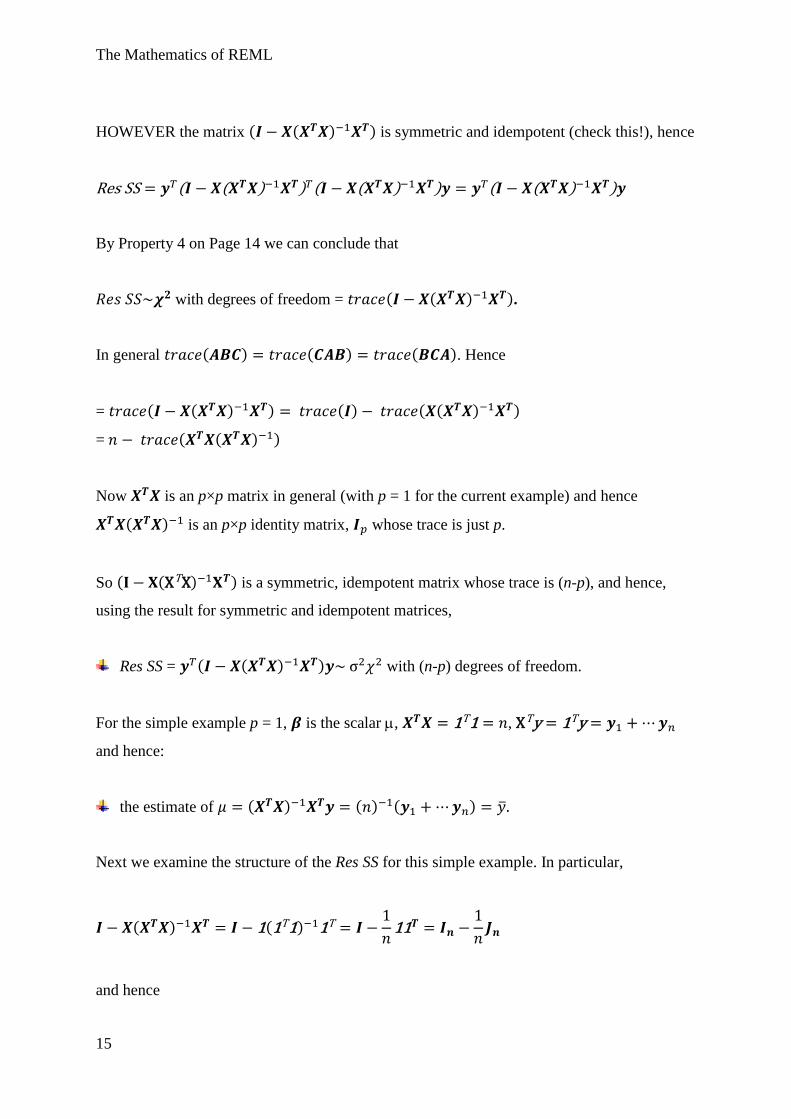
HOWEVER the matrix ( ( ) ) is symmetric and idempotent (check this!), hence
( ( ) ) ( ( ) ) ( ( ) )
By Property 4 on Page 14 we can conclude that
with degrees of freedom = ( ( ) ).
In general ( ) ( ) ( ). Hence
= ( ( ) ) ( ) ( ( ) )
= ( ( ) )
Now is an p×p matrix in general (with p = 1 for the current example) and hence
( ) is an p×p identity matrix, whose trace is just p.
So ( ( ) ) is a symmetric, idempotent matrix whose trace is (n-p), and hence,
using the result for symmetric and idempotent matrices,
Res SS = ( ( ) ) with (n-p) degrees of freedom.
For the simple example p = 1, is the scalar , ,
and hence:
the estimate of ( ) ( ) ( )
Next we examine the structure of the Res SS for this simple example. In particular,
( ) ( )
and hence
The Mathematics of REML
16
( ( ) ) (
)
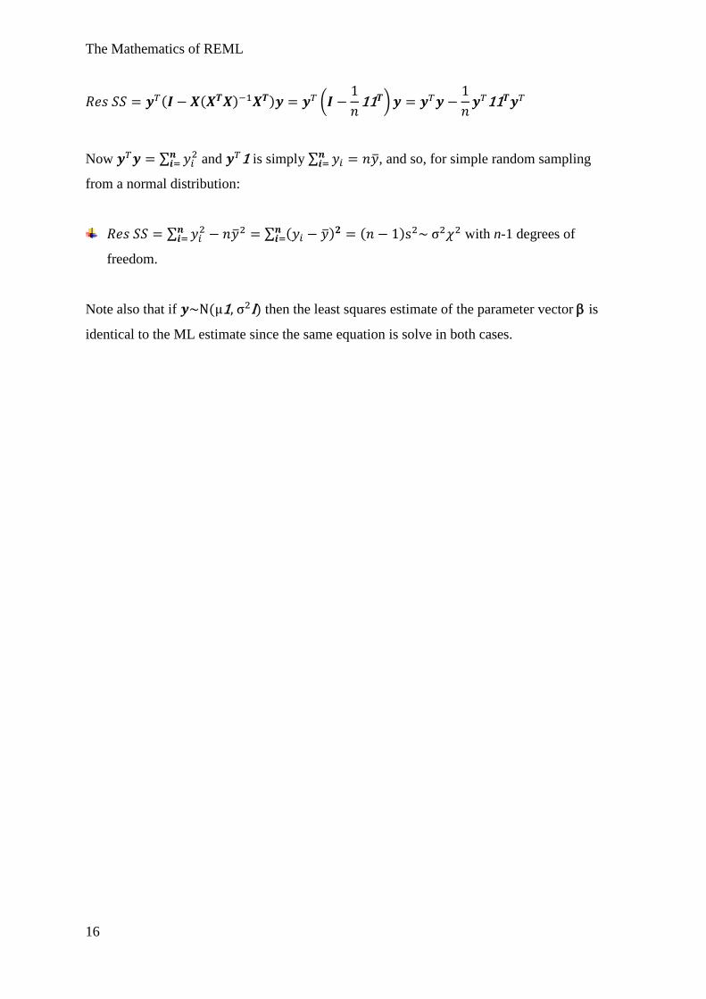
Now ∑
and is simply ∑ , and so, for simple random sampling
from a normal distribution:
∑
∑ ( ) ( ) with n-1 degrees of
freedom.
Note also that if ( ) then the least squares estimate of the parameter vector is
identical to the ML estimate since the same equation is solve in both cases.
The Mathematics of REML
17
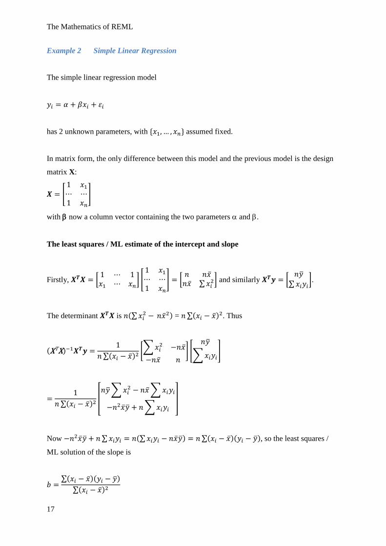
Example 2 Simple Linear Regression
The simple linear regression model
has 2 unknown parameters, with assumed fixed.
In matrix form, the only difference between this model and the previous model is the design
matrix X:
[
]
with now a column vector containing the two parameters and .
The least squares / ML estimate of the intercept and slope
Firstly, [
] [
] [ ∑
] and similarly [
∑ ].
The determinant is (∑ ) = ∑( ) . Thus
( )
∑( ) [∑
] [
∑ ]
∑( ) [ ∑
∑
∑
]
Now ∑ (∑ ) ∑( )( ), so the least squares /
ML solution of the slope is
∑( )( )
∑( )
The Mathematics of REML
18
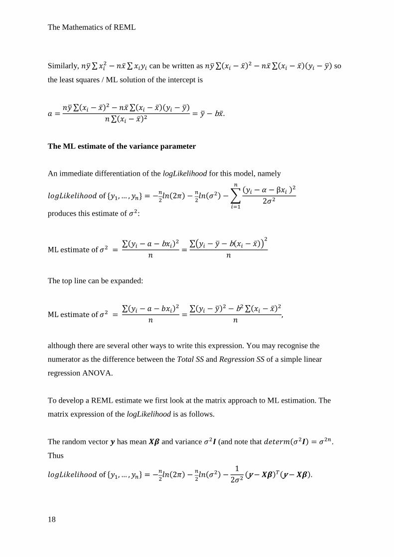
Similarly, ∑ ∑ can be written as ∑( ) ∑( )( ) so
the least squares / ML solution of the intercept is
∑( ) ∑( )( )
∑( )
The ML estimate of the variance parameter
An immediate differentiation of the logLikelihood for this model, namely
( )
( ) ∑
( )
produces this estimate of :
∑( )
∑( ( ))
The top line can be expanded:
∑( )
∑( ) ∑( )
although there are several other ways to write this expression. You may recognise the
numerator as the difference between the Total SS and Regression SS of a simple linear
regression ANOVA.
To develop a REML estimate we first look at the matrix approach to ML estimation. The
matrix expression of the logLikelihood is as follows.
The random vector has mean and variance (and note that ( ) .
Thus
( )
( )
( ) ( )
The Mathematics of REML
19
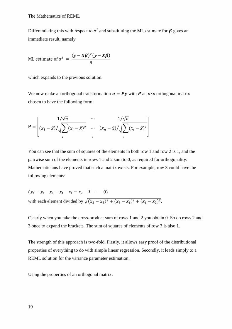
Differentiating this with respect to 2 and substituting the ML estimate for gives an
immediate result, namely
( ) ( )
which expands to the previous solution.
We now make an orthogonal transformation with an n×n orthogonal matrix
chosen to have the following form:
[
√ ⁄ √ ⁄
( ) √∑( ) ⁄ ( ) √∑( ) ⁄
]
You can see that the sum of squares of the elements in both row 1 and row 2 is 1, and the
pairwise sum of the elements in rows 1 and 2 sum to 0, as required for orthogonality.
Mathematicians have proved that such a matrix exists. For example, row 3 could have the
following elements:
( )
with each element divided by √( ) ( ) ( ) .
Clearly when you take the cross-product sum of rows 1 and 2 you obtain 0. So do rows 2 and
3 once to expand the brackets. The sum of squares of elements of row 3 is also 1.
The strength of this approach is two-fold. Firstly, it allows easy proof of the distributional
properties of everything to do with simple linear regression. Secondly, it leads simply to a
REML solution for the variance parameter estimation.
Using the properties of an orthogonal matrix:
The Mathematics of REML
20
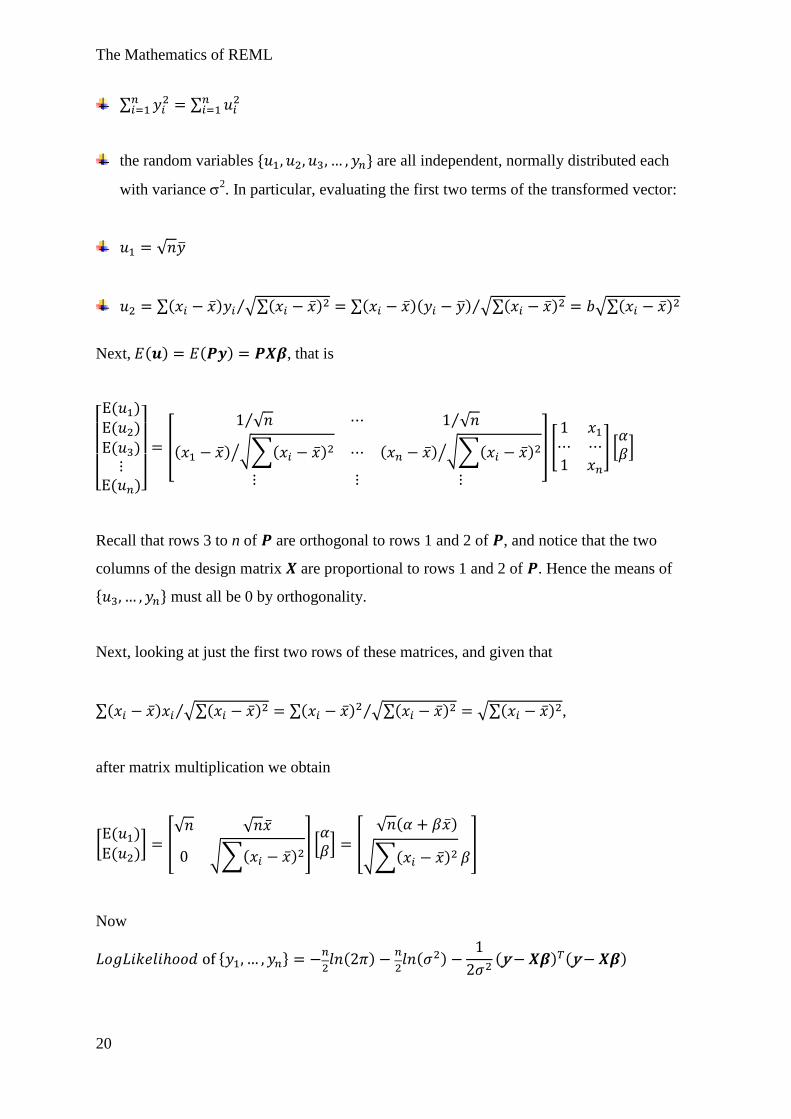
∑
∑
the random variables are all independent, normally distributed each
with variance 2. In particular, evaluating the first two terms of the transformed vector:
√
∑( ) √∑( ) ⁄ ∑( )( ) √∑( ) ⁄ √∑( )
Next, ( ) ( ) , that is
[ ( ) ( ) ( )
( )]
[
√ ⁄ √ ⁄
( ) √∑( ) ⁄ ( ) √∑( ) ⁄
] [
] [ ]
Recall that rows 3 to n of are orthogonal to rows 1 and 2 of , and notice that the two
columns of the design matrix are proportional to rows 1 and 2 of . Hence the means of
must all be 0 by orthogonality.
Next, looking at just the first two rows of these matrices, and given that
∑( ) √∑( ) ⁄ ∑( ) √∑( ) ⁄ √∑( ) ,
after matrix multiplication we obtain
[ ( )
( )] [
√ √
√∑( ) ] [
] [
√ ( )
√∑( ) ]
Now
( )
( )
( ) ( )
The Mathematics of REML
21
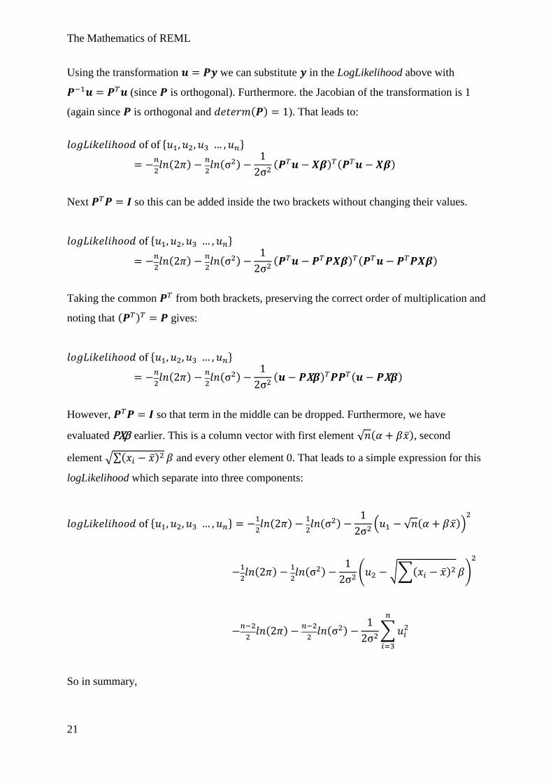
Using the transformation we can substitute in the LogLikelihood above with
(since is orthogonal). Furthermore. the Jacobian of the transformation is 1
(again since is orthogonal and ( ) ). That leads to:
( )
( )
( ) ( )
Next so this can be added inside the two brackets without changing their values.
( )
( )
( ) ( )
Taking the common from both brackets, preserving the correct order of multiplication and
noting that ( ) gives:
( )
( )
( ) ( )
However, so that term in the middle can be dropped. Furthermore, we have
evaluated PX earlier. This is a column vector with first element √ ( ), second
element √∑( ) and every other element 0. That leads to a simple expression for this
logLikelihood which separate into three components:
( )
( )
( √ ( ))
( )
( )
( √∑( ) )
( )
( )
∑
So in summary,
The Mathematics of REML
22
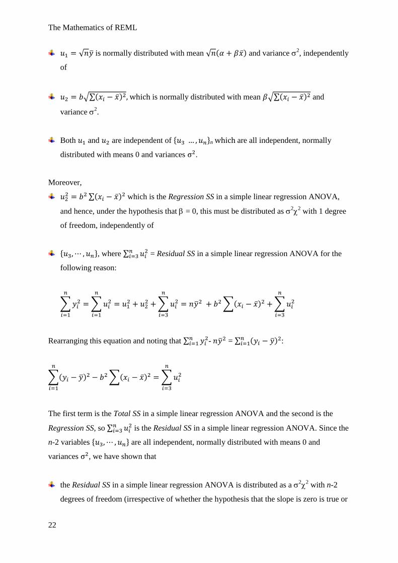
√ is normally distributed with mean √ ( ) and variance 2, independently
of
√∑( ) , which is normally distributed with mean √∑( ) and
variance 2.
Both and are independent of n which are all independent, normally
distributed with means 0 and variances .
Moreover,
∑( ) which is the Regression SS in a simple linear regression ANOVA,
and hence, under the hypothesis that = 0, this must be distributed as 2
2 with 1 degree
of freedom, independently of
, where ∑
= Residual SS in a simple linear regression ANOVA for the
following reason:
∑
∑
∑
∑( ) ∑
Rearranging this equation and noting that ∑
- = ∑ ( ) :
∑( )
∑( ) ∑
The first term is the Total SS in a simple linear regression ANOVA and the second is the
Regression SS, so ∑
is the Residual SS in a simple linear regression ANOVA. Since the
n-2 variables are all independent, normally distributed with means 0 and
variances , we have shown that
the Residual SS in a simple linear regression ANOVA is distributed as a 2
2 with n-2
degrees of freedom (irrespective of whether the hypothesis that the slope is zero is true or
The Mathematics of REML
23
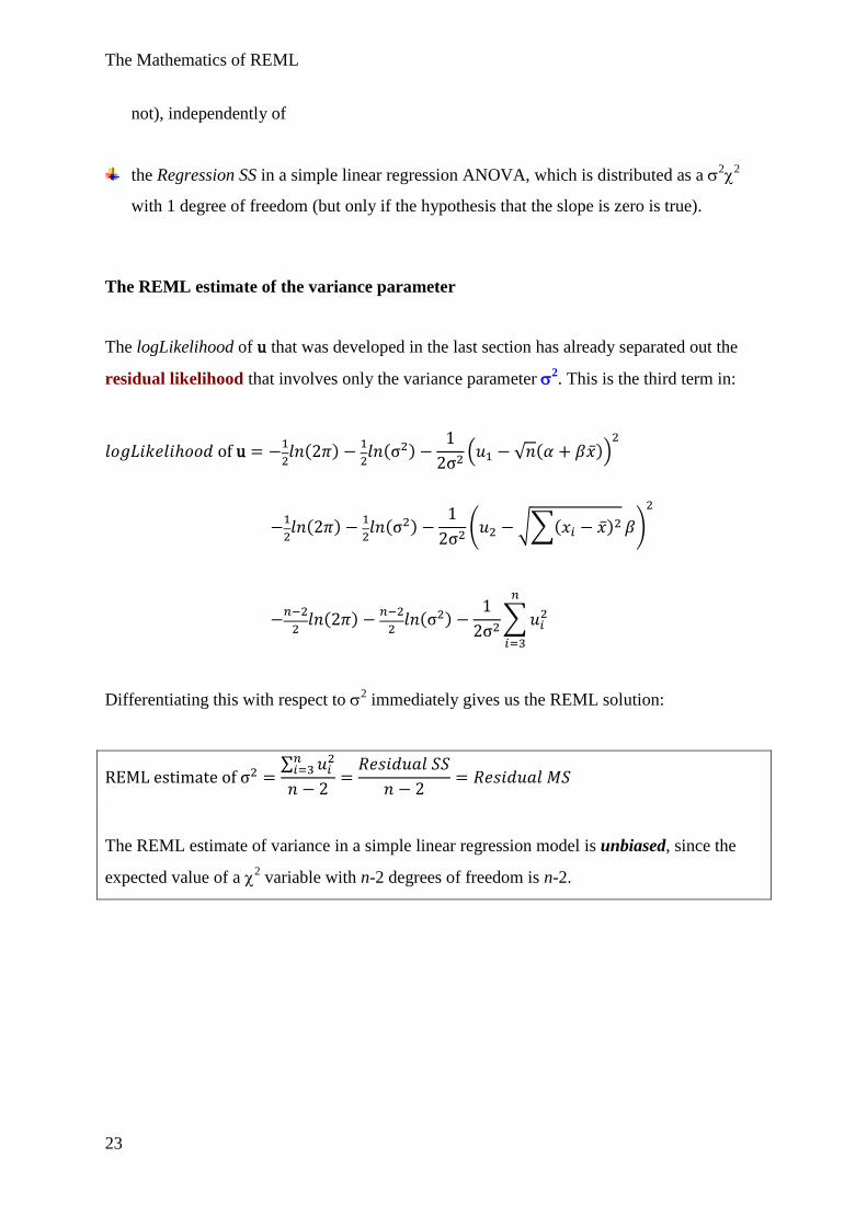
not), independently of
the Regression SS in a simple linear regression ANOVA, which is distributed as a 2
2
with 1 degree of freedom (but only if the hypothesis that the slope is zero is true).
The REML estimate of the variance parameter
The logLikelihood of u that was developed in the last section has already separated out the
residual likelihood that involves only the variance parameter 2. This is the third term in:
( )
( )
( √ ( ))
( )
( )
( √∑( ) )
( )
( )
∑
Differentiating this with respect to 2 immediately gives us the REML solution:
∑
The REML estimate of variance in a simple linear regression model is unbiased, since the
expected value of a 2 variable with n-2 degrees of freedom is n-2.
The Mathematics of REML
24
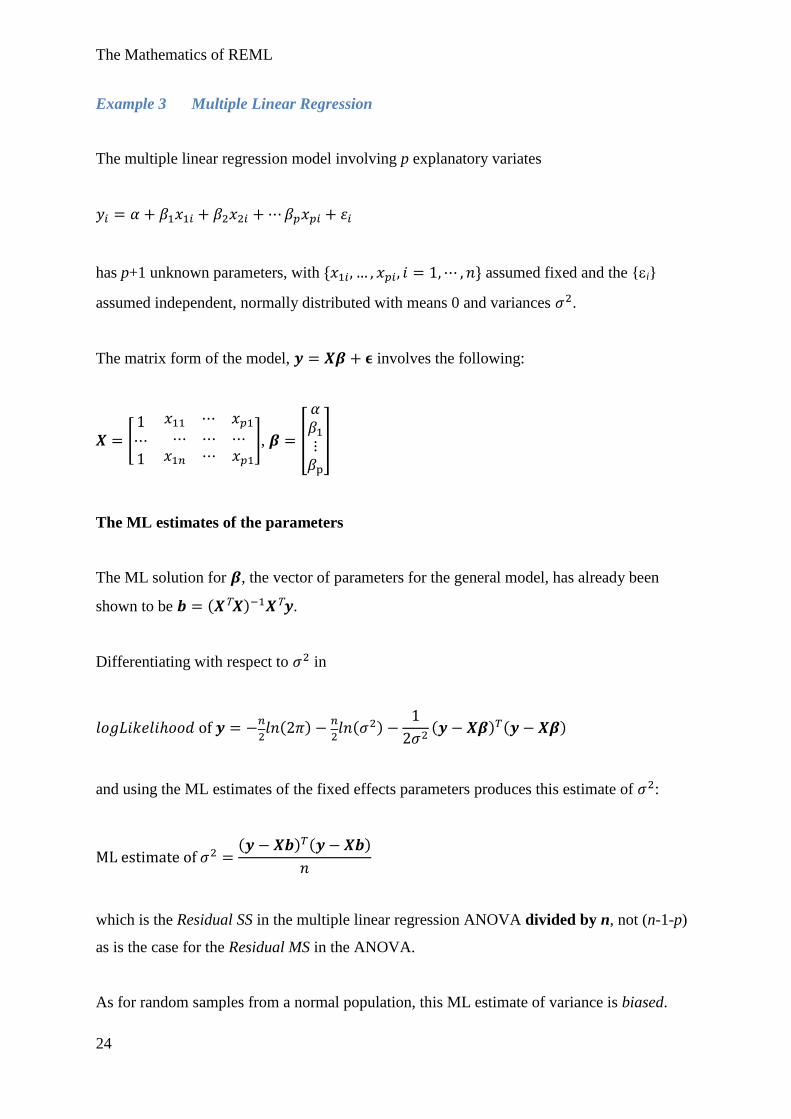
Example 3 Multiple Linear Regression
The multiple linear regression model involving p explanatory variates
has p+1 unknown parameters, with assumed fixed and the {i}
assumed independent, normally distributed with means 0 and variances .
The matrix form of the model, involves the following:
[
], [
]
The ML estimates of the parameters
The ML solution for , the vector of parameters for the general model, has already been
shown to be ( ) .
Differentiating with respect to in
( )
( )
( ) ( )
and using the ML estimates of the fixed effects parameters produces this estimate of :
( ) ( )
which is the Residual SS in the multiple linear regression ANOVA divided by n, not (n-1-p)
as is the case for the Residual MS in the ANOVA.
As for random samples from a normal population, this ML estimate of variance is biased.
The Mathematics of REML
25
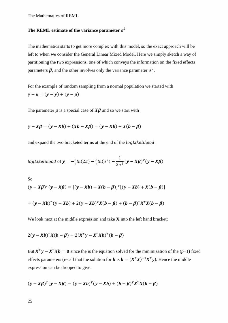
The REML estimate of the variance parameter 2
The mathematics starts to get more complex with this model, so the exact approach will be
left to when we consider the General Linear Mixed Model. Here we simply sketch a way of
partitioning the two expressions, one of which conveys the information on the fixed effects
parameters , and the other involves only the variance parameter .
For the example of random sampling from a normal population we started with
( ) ( )
The parameter is a special case of and so we start with
( ) ( ) ( ) ( )
and expand the two bracketed terms at the end of the :
( )
( )
( ) ( )
So
( ) ( ) [( ) ( )] [( ) ( )]
( ) ( ) ( ) ( ) ( ) ( )
We look next at the middle expression and take X into the left hand bracket:
( ) ( ) ( ) ( )
But since the is the equation solved for the minimization of the (p+1) fixed
effects parameters (recall that the solution for is ( ) ). Hence the middle
expression can be dropped to give:
( ) ( ) ( ) ( ) ( ) ( )
The Mathematics of REML
26
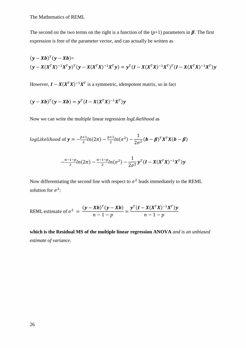
The second on the two terms on the right is a function of the (p+1) parameters in . The first
expression is free of the parameter vector, and can actually be written as
( ) ( )=
( ( ) ) ( ( ) ) ( ( ) ) ( ( ) )
However, ( ) is a symmetric, idempotent matrix, so in fact
( ) ( ) ( ( ) )
Now we can write the multiple linear regression logLikelihood as
( )
( )
( ) ( )
( )
( )
( ( ) )
Now differentiating the second line with respect to leads immediately to the REML
solution for :
( ) ( )
( ( ) )
which is the Residual MS of the multiple linear regression ANOVA and is an unbiased
estimate of variance.
The Mathematics of REML
27
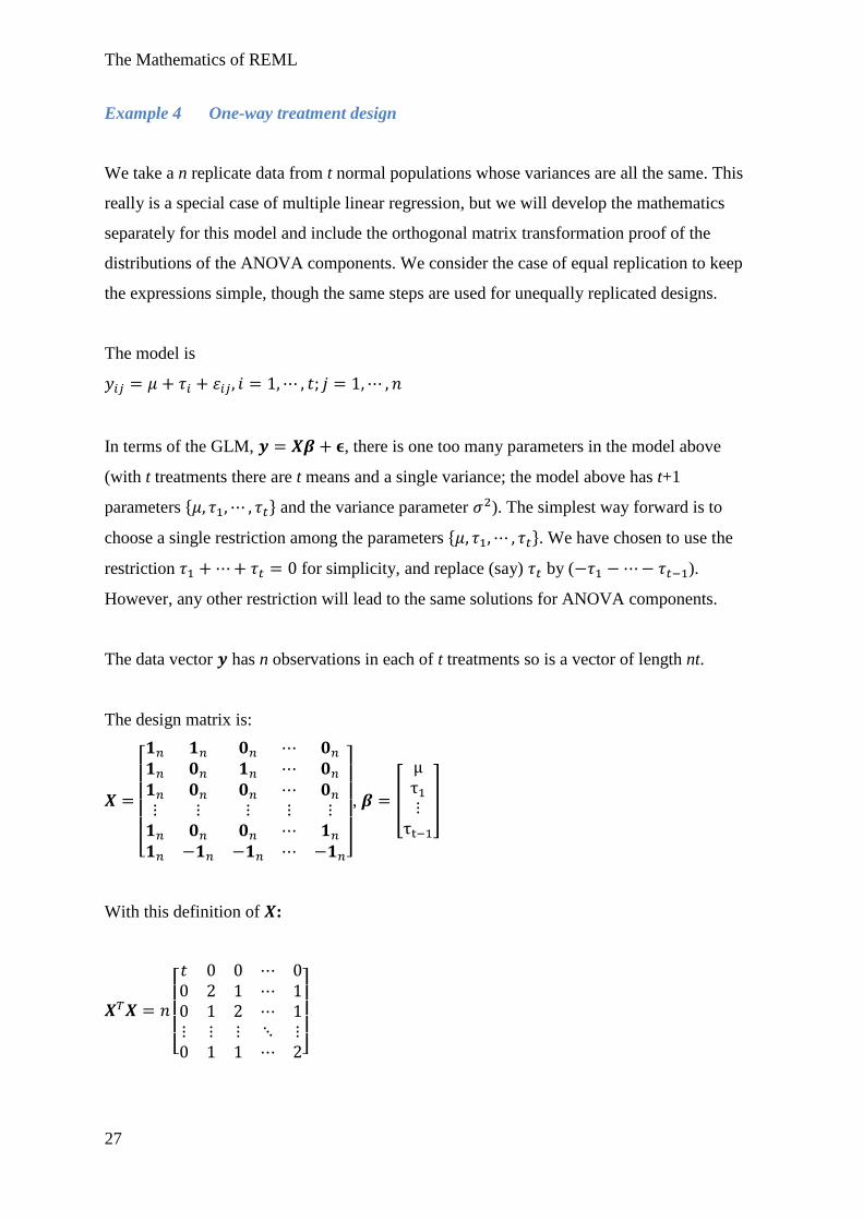
Example 4 One-way treatment design
We take a n replicate data from t normal populations whose variances are all the same. This
really is a special case of multiple linear regression, but we will develop the mathematics
separately for this model and include the orthogonal matrix transformation proof of the
distributions of the ANOVA components. We consider the case of equal replication to keep
the expressions simple, though the same steps are used for unequally replicated designs.
The model is
In terms of the GLM, , there is one too many parameters in the model above
(with t treatments there are t means and a single variance; the model above has t+1
parameters and the variance parameter ). The simplest way forward is to
choose a single restriction among the parameters . We have chosen to use the
restriction for simplicity, and replace (say) by ( ).
However, any other restriction will lead to the same solutions for ANOVA components.
The data vector has n observations in each of t treatments so is a vector of length nt.
The design matrix is:
[
]
, [
]
With this definition of :
[ ]
The Mathematics of REML
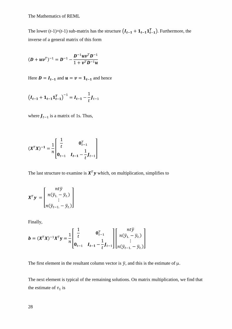
28
The lower (t-1)×(t-1) sub-matrix has the structure ( ). Furthermore, the
inverse of a general matrix of this form
( )
Here and and hence
( )
where is a matrix of 1s. Thus,
( )
[
]
The last structure to examine is which, on multiplication, simplifies to
[
( )
( )
]
Finally,
( )
[
] [
( )
( )
]
The first element in the resultant column vector is , and this is the estimate of .
The next element is typical of the remaining solutions. On matrix multiplication, we find that
the estimate of is
The Mathematics of REML
29
( )
∑( )
( )
∑( )
( )
∑[( ) ( )]
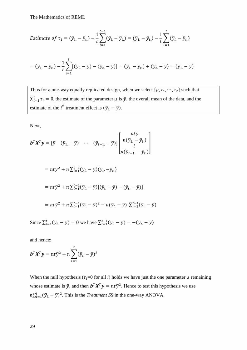
( ) ( ) ( )
Thus for a one-way equally replicated design, when we select such that
∑ the estimate of the parameter is , the overall mean of the data, and the
estimate of the ith
treatment effect is ( ).
Next,
[ ( ) ( )] [
( )
( )
]
∑ ( )( )
∑ ( )[( ) ( )]
∑ ( ) ( ) ∑ ( )
Since ∑ ( ) we have ∑ ( )
( )
and hence:
∑( )
When the null hypothesis ( =0 for all i) holds we have just the one parameter remaining
whose estimate is , and then . Hence to test this hypothesis we use
n∑ ( ) . This is the Treatment SS in the one-way ANOVA.
The Mathematics of REML
30
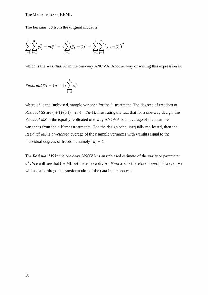
The Residual SS from the original model is
∑∑
∑( )
∑∑( )
which is the in the one-way ANOVA. Another way of writing this expression is:
( )∑
where is the (unbiased) sample variance for the i
th treatment. The degrees of freedom of
Residual SS are (nt-1)-(t-1) = nt-t = t(n-1), illustrating the fact that for a one-way design, the
Residual MS in the equally replicated one-way ANOVA is an average of the t sample
variances from the different treatments. Had the design been unequally replicated, then the
Residual MS is a weighted average of the t sample variances with weights equal to the
individual degrees of freedom, namely ( ).
The Residual MS in the one-way ANOVA is an unbiased estimate of the variance parameter
. We will see that the ML estimate has a divisor N=nt and is therefore biased. However, we
will use an orthogonal transformation of the data in the process.
The Mathematics of REML
31
The ML estimate of the variance parameter 2 for the one-way design
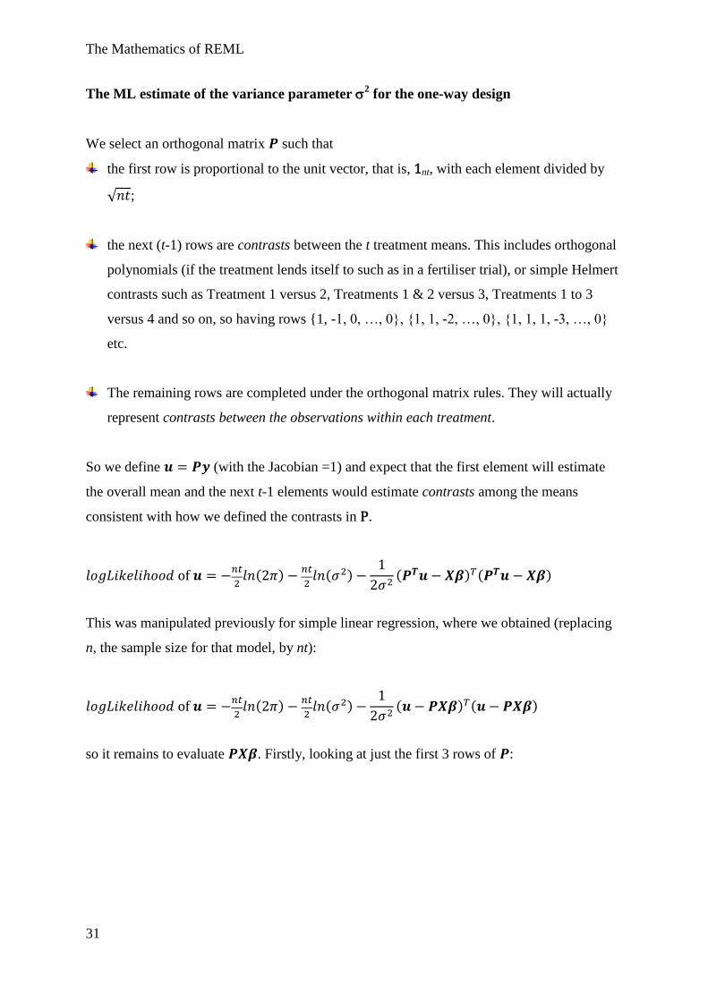
We select an orthogonal matrix such that
the first row is proportional to the unit vector, that is, 1nt, with each element divided by
√ ;
the next (t-1) rows are contrasts between the t treatment means. This includes orthogonal
polynomials (if the treatment lends itself to such as in a fertiliser trial), or simple Helmert
contrasts such as Treatment 1 versus 2, Treatments 1 & 2 versus 3, Treatments 1 to 3
versus 4 and so on, so having rows {1, -1, 0, …, 0}, {1, 1, -2, …, 0}, {1, 1, 1, -3, …, 0}
etc.
The remaining rows are completed under the orthogonal matrix rules. They will actually
represent contrasts between the observations within each treatment.
So we define (with the Jacobian =1) and expect that the first element will estimate
the overall mean and the next t-1 elements would estimate contrasts among the means
consistent with how we defined the contrasts in P.
( )
( )
( ) ( )
This was manipulated previously for simple linear regression, where we obtained (replacing
n, the sample size for that model, by nt):
( )
( )
( ) ( )
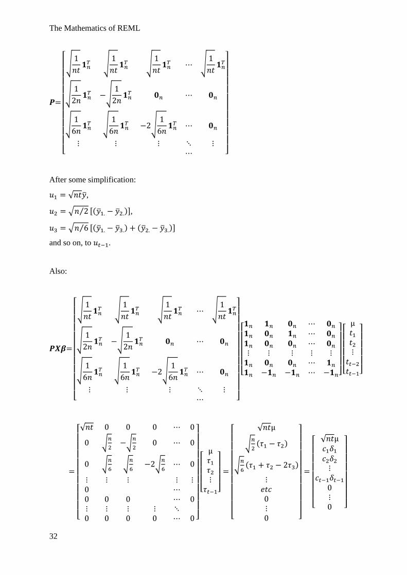
so it remains to evaluate . Firstly, looking at just the first 3 rows of :
The Mathematics of REML
32
[ √
√
√
√
√
√
√
√
√
]
After some simplification:
√ ,
√ ⁄ [( )],
√ ⁄ [( ) ( )]
and so on, to .
Also:
[ √
√
√
√
√
√
√
√
√
]
[
]
[
]
[ √
√
√
√
√
√
]
[
]
[ √
√
( )
√
( )
]
[ √
]
The Mathematics of REML
33
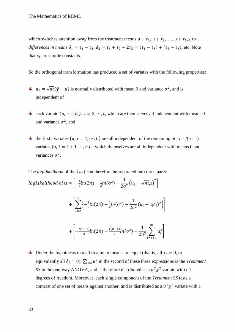
which switches attention away from the treatment means , , …, to
differences in means , ( ) ( ), etc. Note
that are simple constants.
So the orthogonal transformation has produced a set of variates with the following properties:
√ ( ) is normally distributed with mean 0 and variance , and is
independent of
each variate ( ) , which are themselves all independent with means 0
and variance , and
the first t variates are all independent of the remaining nt - t = t(n - 1)
variates which themselves are all independent with means 0 and
variances .
The logLikelihood of the { } can therefore be separated into three parts:
[
( )
( )
( √ )
]
⌈∑{
( )
( )
( )
}
⌉
[ ( )
( )
( )
( )
∑
]
Under the hypothesis that all treatment means are equal (that is, all , or
equivalently all ), ∑
in the second of these three expressions is the Treatment
SS in the one-way ANOVA, and is therefore distributed as a variate with t-1
degrees of freedom. Moreover, each single component of the Treatment SS tests a
contrast of one set of means against another, and is distributed as a variate with 1
The Mathematics of REML
34
degree of freedom.
The final expression in the logLikelihood of the { } involves ∑
, which is the
Residual SS in the one-way ANOVA and is therefore distributed as a variate with
nt-t = t(n-1) degrees of freedom, irrespective of whether the treatment means are all
equal or not. It is also independent of the Treatment SS. Hence
The ratio of Treatment MS to the Residual MS in the one-way ANOVA is, under the
hypothesis that all treatment means are equal, distributed as an F variate with t-1
numerator and t(n-1) denominator degrees of freedom.
Each individual contrast component F value is distributed as an F variate with 1
numerator and t(n-1) denominator degrees of freedom under the assumption that that
particular contrast of treatment means is 0.
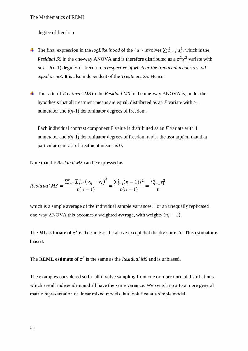
Note that the Residual MS can be expressed as
∑ ∑ ( )
( )
∑ ( )
( )
∑
which is a simple average of the individual sample variances. For an unequally replicated
one-way ANOVA this becomes a weighted average, with weights ( ).
The ML estimate of 2 is the same as the above except that the divisor is tn. This estimator is
biased.
The REML estimate of 2 is the same as the Residual MS and is unbiased.
The examples considered so far all involve sampling from one or more normal distributions
which are all independent and all have the same variance. We switch now to a more general
matrix representation of linear mixed models, but look first at a simple model.
The Mathematics of REML
35
Example 5 - unpaired t tests – equal variances
This is a special case the design considered in the previous example, that is, a one-way
treatment design with no blocking. However we will approach this as a special case to
illustrate why a more general approach is necessary.
For two independent samples taken from normal distributions with different means and the
same variance, we can invoke the properties for simple random samples from a normal
distribution:
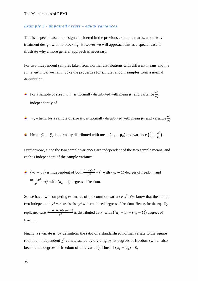
For a sample of size , is normally distributed with mean and variance
,
independently of
, which, for a sample of size , is normally distributed with mean and variance
.
Hence is normally distributed with mean ( ) and variance (
).
Furthermore, since the two sample variances are independent of the two sample means, and
each is independent of the sample variance:
( ) is independent of both ( )
with ( ) degrees of freedom, and
( )
with ( ) degrees of freedom.
So we have two competing estimates of the common variance 2. We know that the sum of
two independent variates is also with combined degrees of freedom. Hence, for the equally
replicated case, ( )
( )
is distributed as with (( ) ( )) degrees of
freedom.
Finally, a t variate is, by definition, the ratio of a standardised normal variate to the square
root of an independent 2 variate scaled by dividing by its degrees of freedom (which also
become the degrees of freedom of the t variate). Thus, if ( ) = 0,
The Mathematics of REML
36
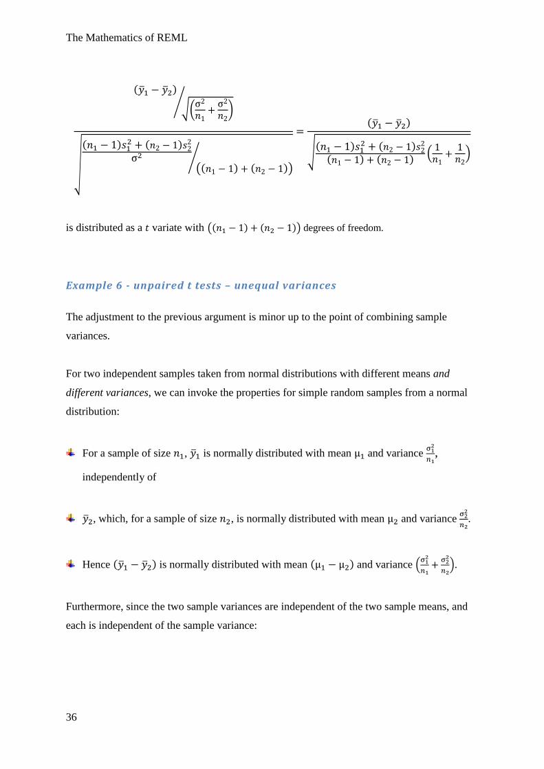
( )
√(
)
⁄
√
( ) ( )
(( ) ( ))⁄
( )
√( )
( )
( ) ( )(
)
is distributed as a variate with (( ) ( )) degrees of freedom.
Example 6 - unpaired t tests – unequal variances
The adjustment to the previous argument is minor up to the point of combining sample
variances.
For two independent samples taken from normal distributions with different means and
different variances, we can invoke the properties for simple random samples from a normal
distribution:
For a sample of size , is normally distributed with mean and variance
,
independently of
, which, for a sample of size , is normally distributed with mean and variance
.
Hence ( ) is normally distributed with mean ( ) and variance (
).
Furthermore, since the two sample variances are independent of the two sample means, and
each is independent of the sample variance:
The Mathematics of REML
37
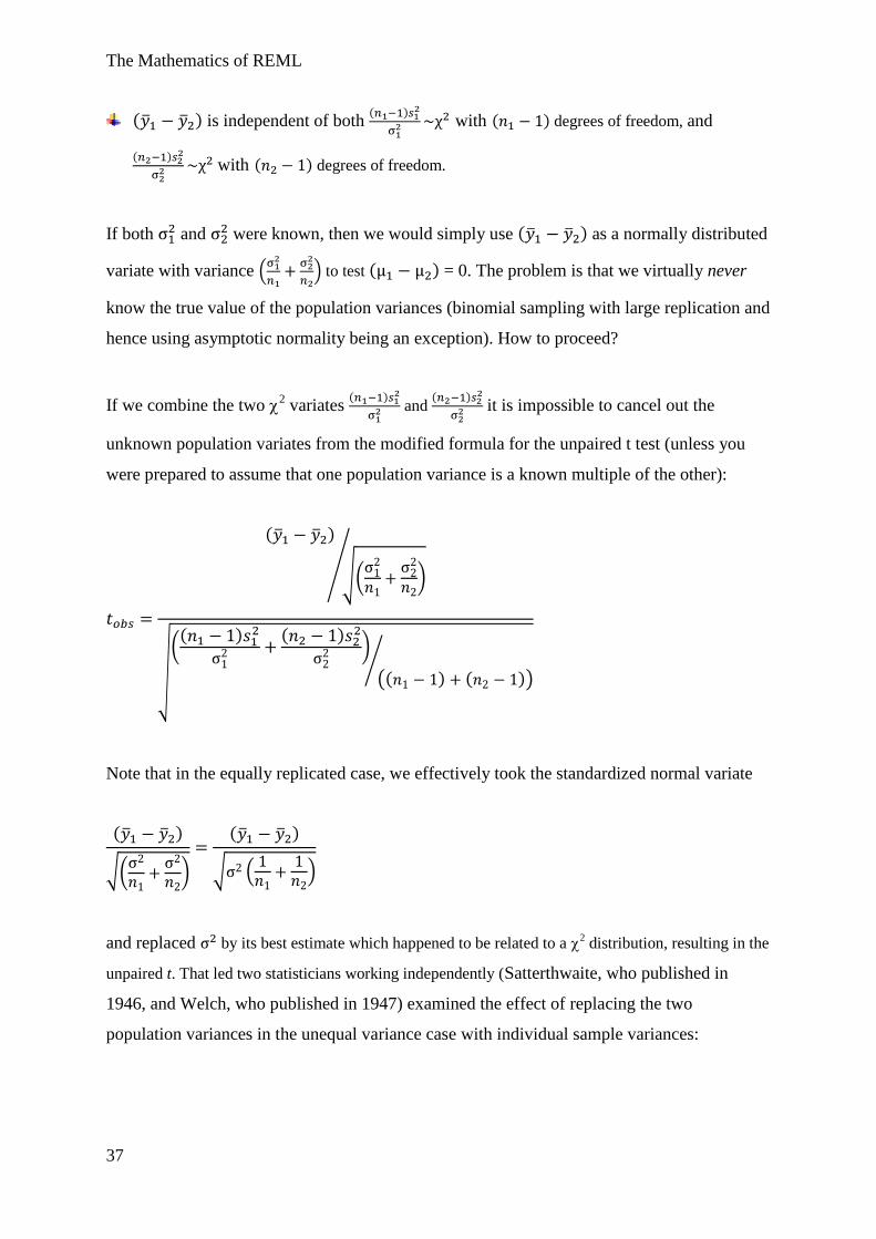
( ) is independent of both ( )
with ( ) degrees of freedom, and
( )
with ( ) degrees of freedom.
If both and
were known, then we would simply use ( ) as a normally distributed
variate with variance (
) to test ( ) = 0. The problem is that we virtually never
know the true value of the population variances (binomial sampling with large replication and
hence using asymptotic normality being an exception). How to proceed?
If we combine the two 2 variates
( )
and
( )
it is impossible to cancel out the
unknown population variates from the modified formula for the unpaired t test (unless you
were prepared to assume that one population variance is a known multiple of the other):
( )
√(
)
⁄
√
(( )
( )
)
(( ) ( ))⁄
Note that in the equally replicated case, we effectively took the standardized normal variate
( )
√(
)
( )
√ (
)
and replaced by its best estimate which happened to be related to a 2 distribution, resulting in the
unpaired t. That led two statisticians working independently (Satterthwaite, who published in
1946, and Welch, who published in 1947) examined the effect of replacing the two
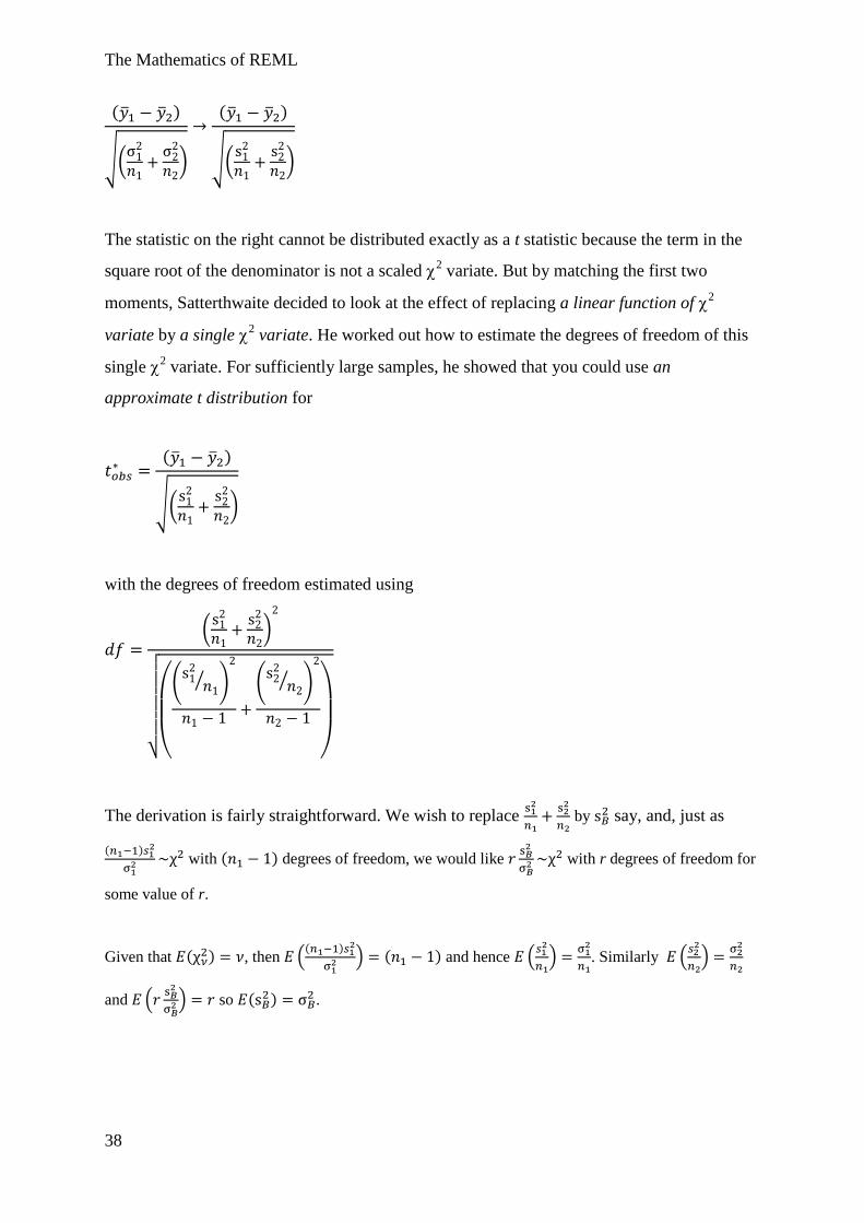
population variances in the unequal variance case with individual sample variances:
The Mathematics of REML
38
( )
√(
)
( )
√(
)
The statistic on the right cannot be distributed exactly as a t statistic because the term in the
square root of the denominator is not a scaled 2 variate. But by matching the first two
moments, Satterthwaite decided to look at the effect of replacing a linear function of 2
variate by a single 2 variate. He worked out how to estimate the degrees of freedom of this
single 2 variate. For sufficiently large samples, he showed that you could use an
approximate t distribution for
( )
√(
)
with the degrees of freedom estimated using
(
)
√
(
(
⁄ )
(
⁄ )
)
The derivation is fairly straightforward. We wish to replace
by
say, and, just as
( )
with ( ) degrees of freedom, we would like
with r degrees of freedom for
some value of r.
Given that ( ) , then (
( )
) ( ) and hence (
)
. Similarly (
)
and (
) so (
) .
The Mathematics of REML
39
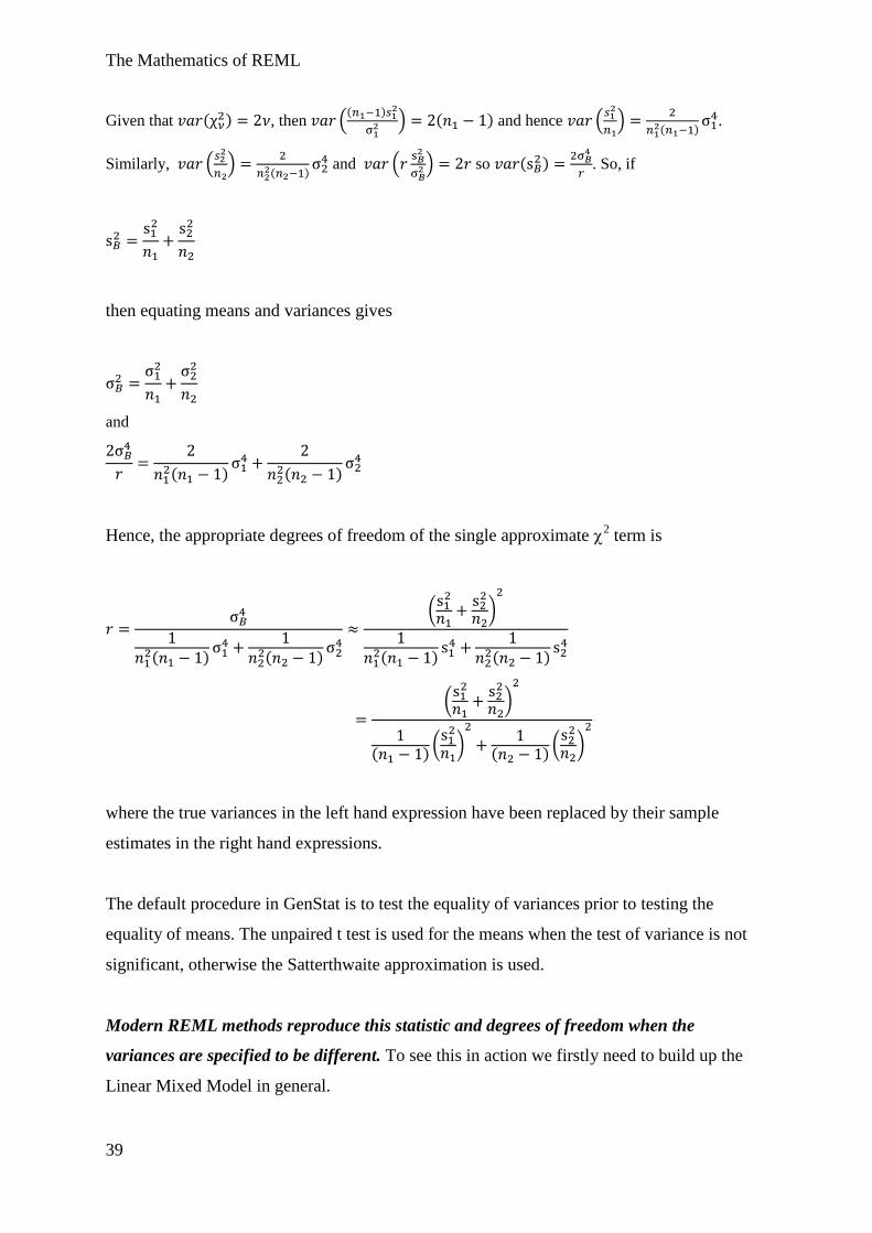
Given that ( ) , then (
( )
) ( ) and hence (
)
( )
.
Similarly, (
)
( )
and (
) so (
)
. So, if
then equating means and variances gives
and
( )
( )
Hence, the appropriate degrees of freedom of the single approximate 2 term is
( )
( )
(
)
( )
( )
(
)
( )
(
)
( )(
)
where the true variances in the left hand expression have been replaced by their sample
estimates in the right hand expressions.
The default procedure in GenStat is to test the equality of variances prior to testing the
equality of means. The unpaired t test is used for the means when the test of variance is not
significant, otherwise the Satterthwaite approximation is used.
Modern REML methods reproduce this statistic and degrees of freedom when the
variances are specified to be different. To see this in action we firstly need to build up the
Linear Mixed Model in general.
The Mathematics of REML
40
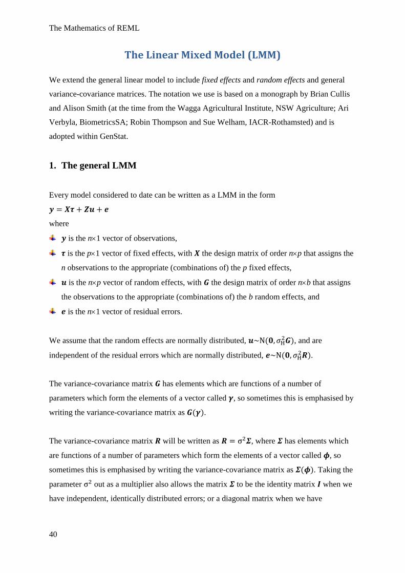
The Linear Mixed Model (LMM)
We extend the general linear model to include fixed effects and random effects and general
variance-covariance matrices. The notation we use is based on a monograph by Brian Cullis
and Alison Smith (at the time from the Wagga Agricultural Institute, NSW Agriculture; Ari
Verbyla, BiometricsSA; Robin Thompson and Sue Welham, IACR-Rothamsted) and is
adopted within GenStat.
1. The general LMM
Every model considered to date can be written as a LMM in the form
where
is the n1 vector of observations,
is the p1 vector of fixed effects, with the design matrix of order np that assigns the
n observations to the appropriate (combinations of) the p fixed effects,
is the np vector of random effects, with the design matrix of order nb that assigns
the observations to the appropriate (combinations of) the b random effects, and
is the n1 vector of residual errors.
We assume that the random effects are normally distributed, ( ), and are
independent of the residual errors which are normally distributed, ( ).
The variance-covariance matrix has elements which are functions of a number of
parameters which form the elements of a vector called , so sometimes this is emphasised by
writing the variance-covariance matrix as ( ).
The variance-covariance matrix will be written as , where has elements which
are functions of a number of parameters which form the elements of a vector called , so
sometimes this is emphasised by writing the variance-covariance matrix as ( ). Taking the
parameter out as a multiplier also allows the matrix to be the identity matrix when we
have independent, identically distributed errors; or a diagonal matrix when we have
The Mathematics of REML
41
independent errors but changing variance; or a correlation matrix when we have correlated
errors but constant variance.
We have seen special cases of the LMM in the previous examples:
For simple random sampling from a normal population we have one fixed parameter only
and = () is a scalar which applies to every observation; hence is the unit vector 1n.
There are no other random effects, hence .
For simple linear regression there are two fixed effects (the intercept and slope) so
T = (, ) and = (1n, x) where x is the vector of explanatory variates. There are no
other random effects, hence .
For a one-way fixed treatment design with no blocks and t treatments there are t fixed
effects: t means, so T = (1, ..., t); or an overall mean plus t-1 treatment effects, so
T = (, 1, ..., t-1); or any other parameterisation of the t treatments. Then is the design
matrix identifying which treatment each observation belongs to. There are no other
random effects, hence .
Notice that instead of a set of fixed treatments of interest, we could have randomly
selected and t treatments from a large population of treatments, in which case these
become a random treatment effect and will appear as in which case is the design
matrix identifying which treatment each observation belongs to. We will consider this
type of experiment later.
Since and have zero mean vectors the mean of the data vector is ( ) and its
variance-covariance matrix is
( ) ( )( ) ( )( ) ( )( )
( )
where and is a scaling factor that allows the and structures to be
expressed as variance or correlation models in some instances.
The Mathematics of REML
42
Thus the distribution of the data vector is normal with mean and variance-covariance
matrix .
2. Transforming to segregate the fixed effects
This next step in the REML estimation is similar to what we have done to date with
orthogonal transformations, though we don’t need every matrix to be orthogonal.
So, we take the data vector y and find transformation of y to [
] where the matrix
[ ] consists of two specially chosen sub-matrices, just as we chose special
orthogonal matrices for the different examples earlier in the manual: an n×p matrix and an
n×(n-p) matrix . There are two properties we need for these sub-matrices, namely (and
remember that there are p fixed effects in the LMM):
Condition 1:
Condition 2:
Under these conditions:
(
) since
( ) ( )
by choice of , and
( ) ( )
(
) since
( ) ( )
by choice of , and
( ) ( )
( ) ( )
The Mathematics of REML
43
Summary to date: Using this transformation,
[
] ([
]
[
])
The next step requires general properties of conditional distributions of multivariate normal
variables. Specifically, let
[
] ([
] [
])
Note that, as a covariance matrix, (1) and must be symmetric, and (2) .
Then the conditional distribution of given is:
| ( ( )
)
We now apply this general result to the variates and whose means and variance
matrices given on the previous page. The result appears complex, however it can be further
simplified.
| ( (
)
[
( )
])
How does this simplification work? The mathematics is not easy, and there are several ways
to generate the result. We start by considering a new matrix whose inverse can be shown to
exist.
So, consider the n×n matrix [ ] where is an n×p matrix and is an n×(n-p)
matrix with and
as defined earlier. Next, consider this matrix product:
[ ] ([ ]
) ([ ] [ ])
([
] [ ])
(and now absorbing the H matrix in the middle into the left hand matrix)
([
] [ ])
The Mathematics of REML
44
[
]
[
]
[( )
( )
]
Now we rearrange this equality be pre- and post- multiplication to leave H-1
on the left hand
side of the equation:
[( )
( )
] [ ]
[ ( ) ( )
][ ]
( ) ( )
FINALLY, pre-multiply throughout by and post-multiply by to obtain
( ) (
)
The LHS is and hence, on simplification of the RHS,
( ) ( )(
) (
)
However, we started with and so
( ) (
)( )
( )
which leads to what we set out to prove, namely that, for these choices of and ,
(
)( )
( ) ( )
and since we are conditioning on , if we define the fixed (
) as
, we
have the more simple statement:
| (
( ) )
The Mathematics of REML
45
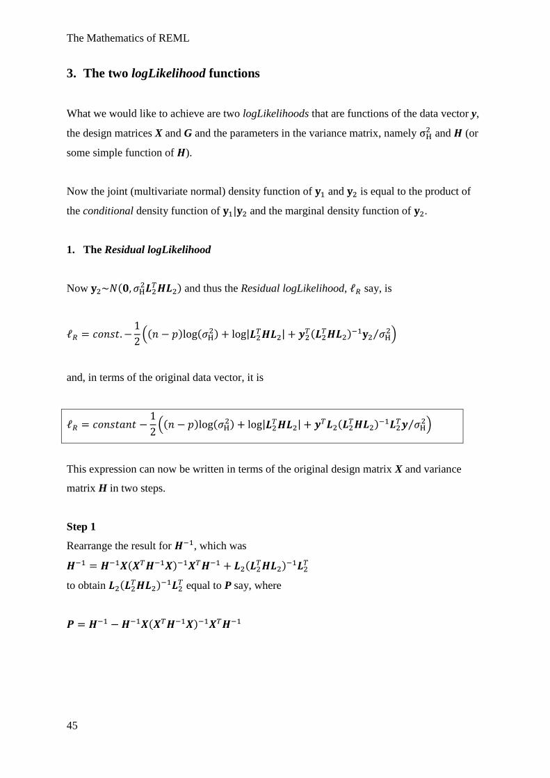
3. The two logLikelihood functions
What we would like to achieve are two logLikelihoods that are functions of the data vector y,
the design matrices X and G and the parameters in the variance matrix, namely and (or
some simple function of ).
Now the joint (multivariate normal) density function of and is equal to the product of
the conditional density function of | and the marginal density function of .
1. The Residual logLikelihood
Now (
) and thus the Residual logLikelihood, say, is
(( ) (
) | |
( )
⁄ )
and, in terms of the original data vector, it is
(( ) (
) | | (
)
⁄ )
This expression can now be written in terms of the original design matrix X and variance
matrix H in two steps.
Step 1
Rearrange the result for , which was
( ) ( )
to obtain ( )
equal to P say, where
( )
The Mathematics of REML
46
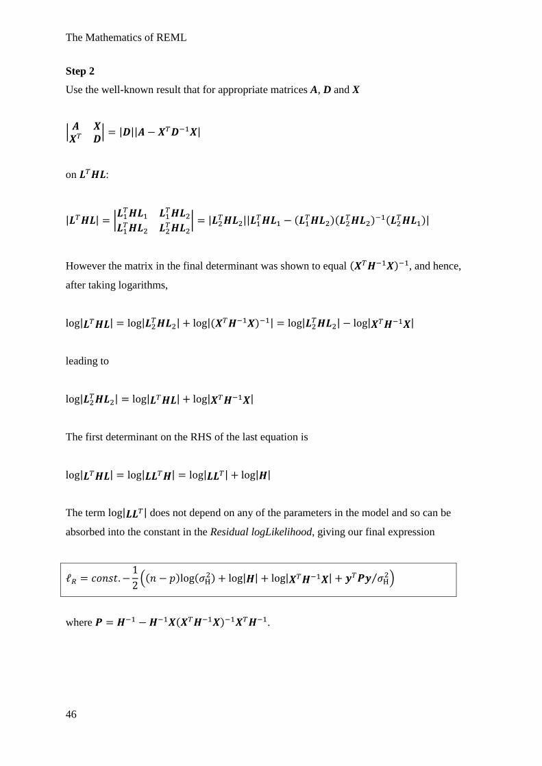
Step 2
Use the well-known result that for appropriate matrices A, D and X
|
| | || |
on :
| | |
| | ||
( )(
) (
)|
However the matrix in the final determinant was shown to equal ( ) , and hence,
after taking logarithms,
| | | | |( ) | |
| | |
leading to
| | | | | |
The first determinant on the RHS of the last equation is
| | | | | | | |
The term | | does not depend on any of the parameters in the model and so can be
absorbed into the constant in the Residual logLikelihood, giving our final expression
(( ) (
) | | | | ⁄ )
where ( ) .
The Mathematics of REML
47
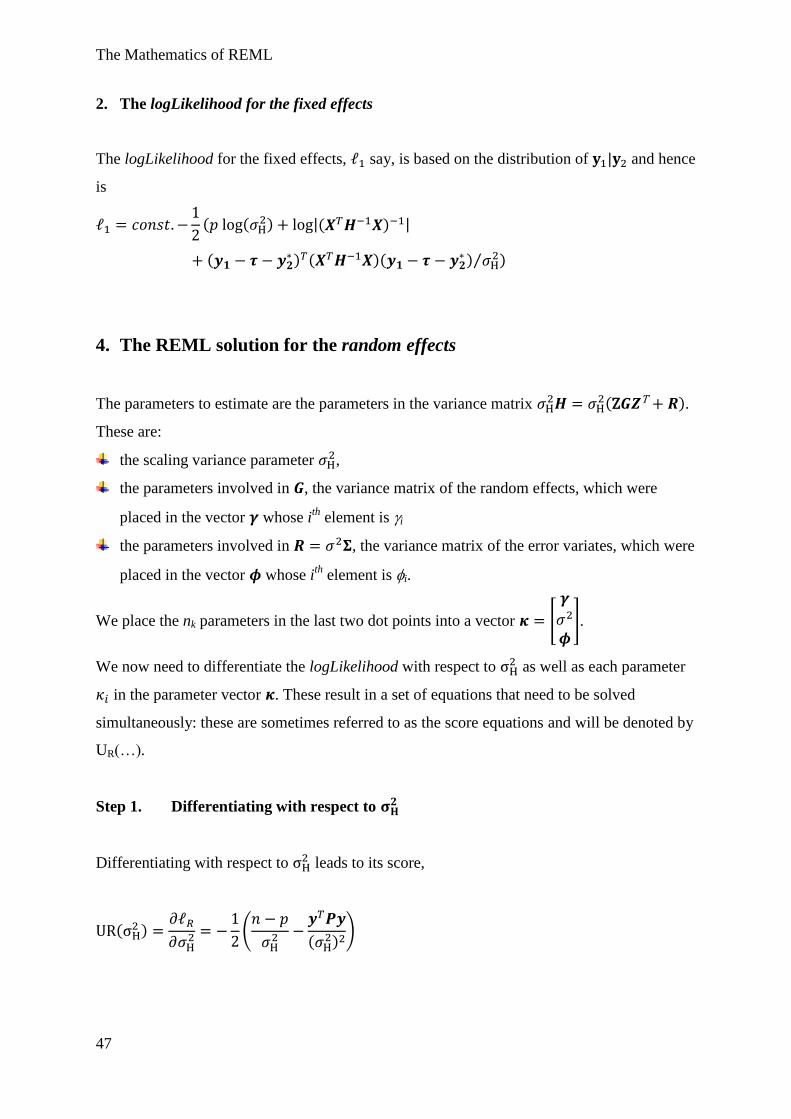
2. The logLikelihood for the fixed effects
The logLikelihood for the fixed effects, say, is based on the distribution of | and hence
is
( (
) |( ) |
( ) ( )(
) ⁄ )
4. The REML solution for the random effects
The parameters to estimate are the parameters in the variance matrix
( ).
These are:
the scaling variance parameter ,
the parameters involved in , the variance matrix of the random effects, which were
placed in the vector whose ith
element is i
the parameters involved in , the variance matrix of the error variates, which were
placed in the vector whose ith
element is i.
We place the nk parameters in the last two dot points into a vector [
].
We now need to differentiate the logLikelihood with respect to as well as each parameter
in the parameter vector . These result in a set of equations that need to be solved
simultaneously: these are sometimes referred to as the score equations and will be denoted by
UR(…).
Step 1. Differentiating with respect to
Differentiating with respect to leads to its score,
( )
(
( )
)
The Mathematics of REML
48
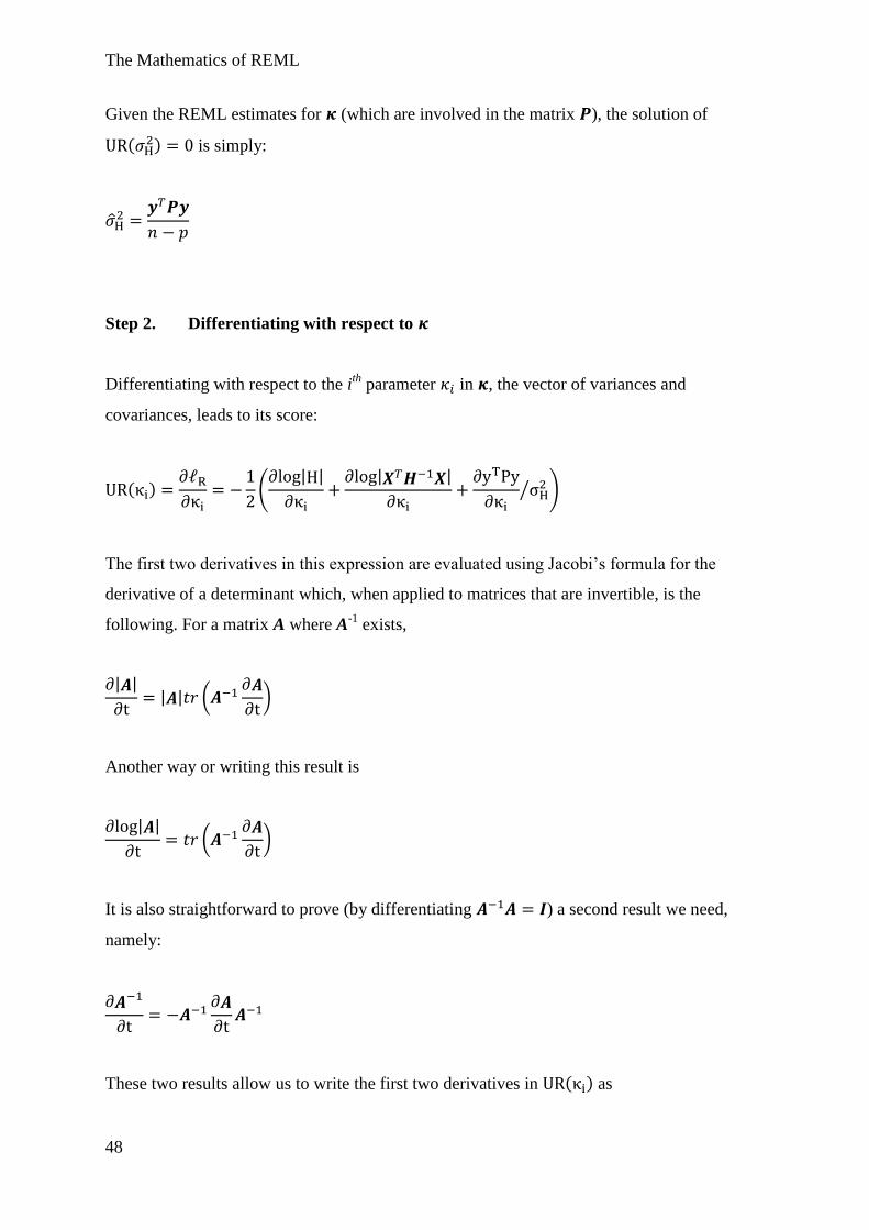
Given the REML estimates for (which are involved in the matrix ), the solution of
( ) is simply:
Step 2. Differentiating with respect to
Differentiating with respect to the ith
parameter in , the vector of variances and
covariances, leads to its score:
( )
( | |
| |
⁄ )
The first two derivatives in this expression are evaluated using Jacobi’s formula for the
derivative of a determinant which, when applied to matrices that are invertible, is the
following. For a matrix A where A-1
exists,
| |
| | (
)
Another way or writing this result is
| |
(
)
It is also straightforward to prove (by differentiating ) a second result we need,
namely:
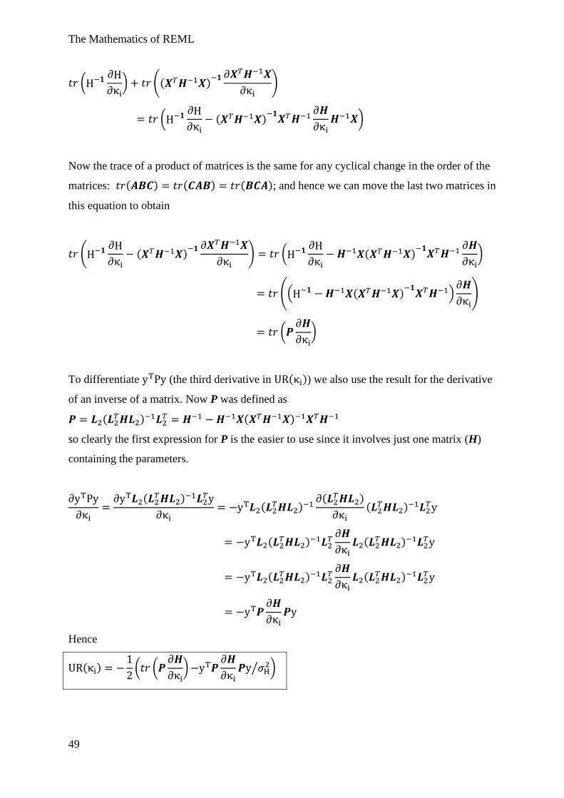
These two results allow us to write the first two derivatives in ( ) as
The Mathematics of REML
49
(
) (( )
)
(
( )
)
Now the trace of a product of matrices is the same for any cyclical change in the order of the
matrices: ( ) ( ) ( ); and hence we can move the last two matrices in
this equation to obtain
(
( )
) (
( )
)
(( ( )
)
)
(
)
To differentiate (the third derivative in ( )) we also use the result for the derivative
of an inverse of a matrix. Now P was defined as
( )
( )
so clearly the first expression for P is the easier to use since it involves just one matrix (H)
containing the parameters.
( )
(
)
( )
( )
( )
(
)
( )
(
)
Hence
( )
( (
)
⁄ )
The Mathematics of REML
50
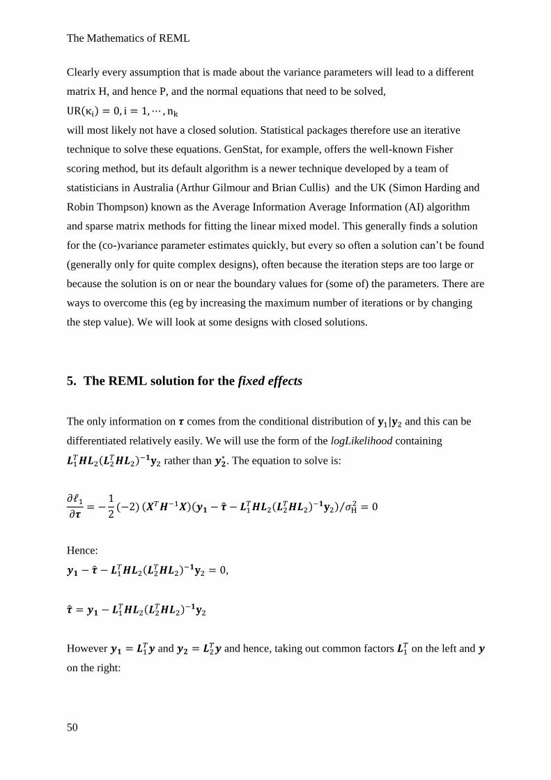
Clearly every assumption that is made about the variance parameters will lead to a different
matrix H, and hence P, and the normal equations that need to be solved,
( )
will most likely not have a closed solution. Statistical packages therefore use an iterative
technique to solve these equations. GenStat, for example, offers the well-known Fisher
scoring method, but its default algorithm is a newer technique developed by a team of
statisticians in Australia (Arthur Gilmour and Brian Cullis) and the UK (Simon Harding and
Robin Thompson) known as the Average Information Average Information (AI) algorithm
and sparse matrix methods for fitting the linear mixed model. This generally finds a solution
for the (co-)variance parameter estimates quickly, but every so often a solution can’t be found
(generally only for quite complex designs), often because the iteration steps are too large or
because the solution is on or near the boundary values for (some of) the parameters. There are
ways to overcome this (eg by increasing the maximum number of iterations or by changing
the step value). We will look at some designs with closed solutions.
5. The REML solution for the fixed effects
The only information on comes from the conditional distribution of | and this can be
differentiated relatively easily. We will use the form of the logLikelihood containing
(
) rather than
. The equation to solve is:
( ) ( )(
( )
) ⁄
Hence:
(
) ,
(
)
However and
and hence, taking out common factors on the left and
on the right:
The Mathematics of REML
51
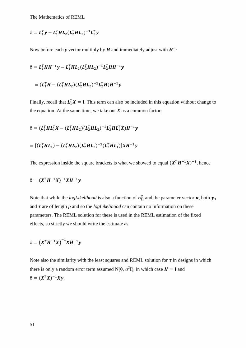
( )
Now before each y vector multiply by H and immediately adjust with H-1
:
( )
( (
)( )
)
Finally, recall that . This term can also be included in this equation without change to
the equation. At the same time, we take out X as a common factor:
(
( )(
)
)
[( ) (
)( )
( )]
The expression inside the square brackets is what we showed to equal ( ) , hence
( )
Note that while the logLikelihood is also a function of and the parameter vector , both
and are of length p and so the logLikelihood can contain no information on these
parameters. The REML solution for these is used in the REML estimation of the fixed
effects, so strictly we should write the estimate as
( )
Note also the similarity with the least squares and REML solution for in designs in which
there is only a random error term assumed N(0, 2I), in which case and
( ) .
The Mathematics of REML
52
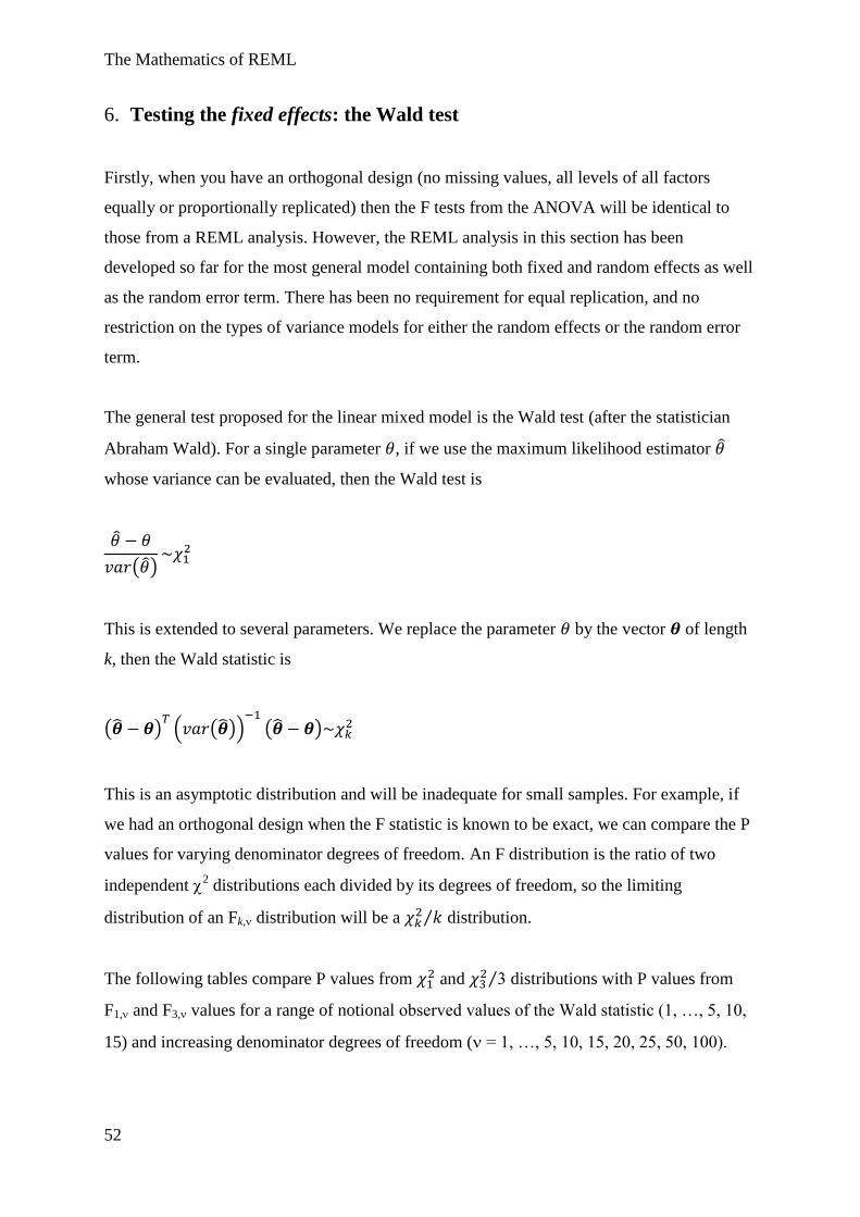
6. Testing the fixed effects: the Wald test
Firstly, when you have an orthogonal design (no missing values, all levels of all factors
equally or proportionally replicated) then the F tests from the ANOVA will be identical to
those from a REML analysis. However, the REML analysis in this section has been
developed so far for the most general model containing both fixed and random effects as well
as the random error term. There has been no requirement for equal replication, and no
restriction on the types of variance models for either the random effects or the random error
term.
The general test proposed for the linear mixed model is the Wald test (after the statistician
Abraham Wald). For a single parameter , if we use the maximum likelihood estimator
whose variance can be evaluated, then the Wald test is
( )
This is extended to several parameters. We replace the parameter by the vector of length
k, then the Wald statistic is
( ) ( ( ))
( )
This is an asymptotic distribution and will be inadequate for small samples. For example, if
we had an orthogonal design when the F statistic is known to be exact, we can compare the P
values for varying denominator degrees of freedom. An F distribution is the ratio of two
independent 2 distributions each divided by its degrees of freedom, so the limiting
distribution of an Fk, distribution will be a ⁄ distribution.
The following tables compare P values from and
3⁄ distributions with P values from
F1, and F3, values for a range of notional observed values of the Wald statistic (1, …, 5, 10,
15) and increasing denominator degrees of freedom ( = 1, …, 5, 10, 15, 20, 25, 50, 100).
The Mathematics of REML
53
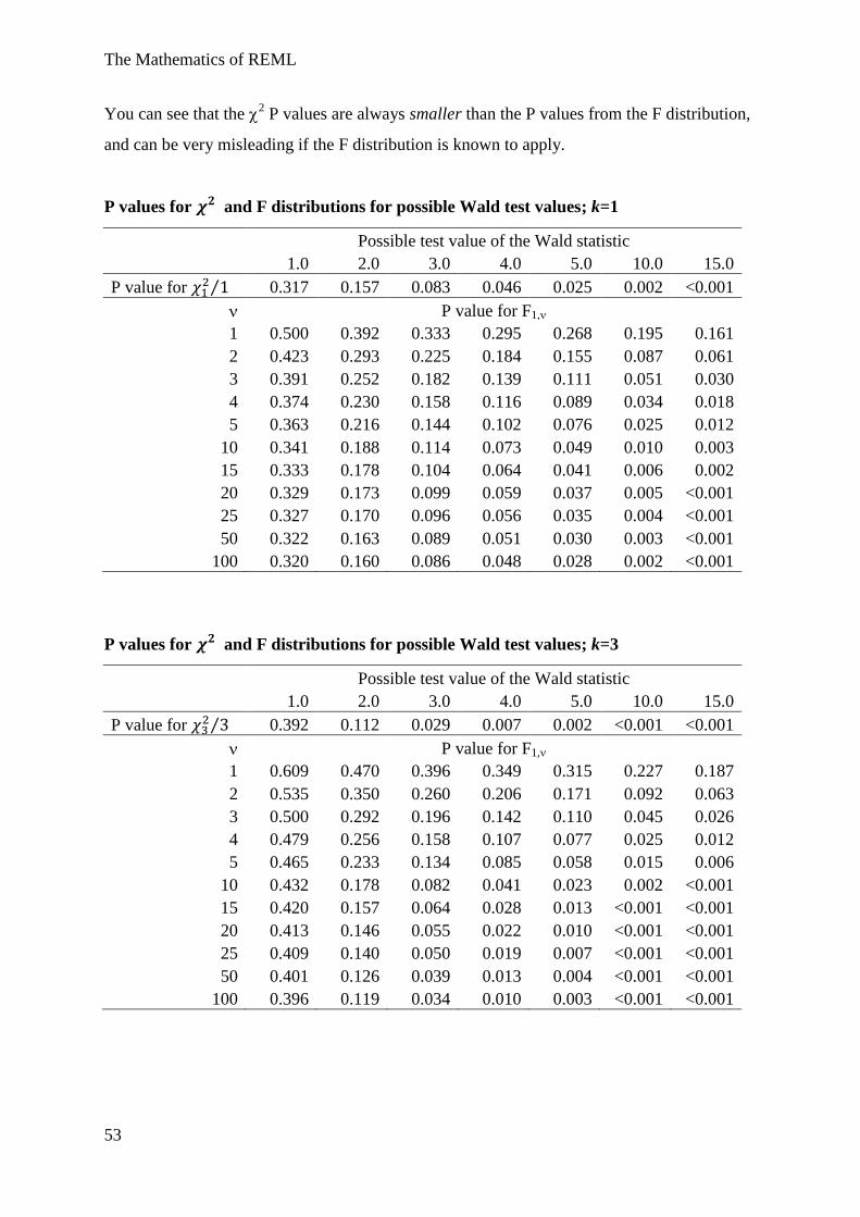
You can see that the 2 P values are always smaller than the P values from the F distribution,
and can be very misleading if the F distribution is known to apply.
P values for and F distributions for possible Wald test values; k=1
Possible test value of the Wald statistic
1.0 2.0 3.0 4.0 5.0 10.0 15.0
P value for ⁄ 0.317 0.157 0.083 0.046 0.025 0.002 <0.001
P value for F1,
1 0.500 0.392 0.333 0.295 0.268 0.195 0.161
2 0.423 0.293 0.225 0.184 0.155 0.087 0.061
3 0.391 0.252 0.182 0.139 0.111 0.051 0.030
4 0.374 0.230 0.158 0.116 0.089 0.034 0.018
5 0.363 0.216 0.144 0.102 0.076 0.025 0.012
10 0.341 0.188 0.114 0.073 0.049 0.010 0.003
15 0.333 0.178 0.104 0.064 0.041 0.006 0.002
20 0.329 0.173 0.099 0.059 0.037 0.005 <0.001
25 0.327 0.170 0.096 0.056 0.035 0.004 <0.001
50 0.322 0.163 0.089 0.051 0.030 0.003 <0.001
100 0.320 0.160 0.086 0.048 0.028 0.002 <0.001
P values for and F distributions for possible Wald test values; k=3
Possible test value of the Wald statistic
1.0 2.0 3.0 4.0 5.0 10.0 15.0
P value for ⁄ 0.392 0.112 0.029 0.007 0.002 <0.001 <0.001
P value for F1,
1 0.609 0.470 0.396 0.349 0.315 0.227 0.187
2 0.535 0.350 0.260 0.206 0.171 0.092 0.063
3 0.500 0.292 0.196 0.142 0.110 0.045 0.026
4 0.479 0.256 0.158 0.107 0.077 0.025 0.012
5 0.465 0.233 0.134 0.085 0.058 0.015 0.006
10 0.432 0.178 0.082 0.041 0.023 0.002 <0.001
15 0.420 0.157 0.064 0.028 0.013 <0.001 <0.001
20 0.413 0.146 0.055 0.022 0.010 <0.001 <0.001
25 0.409 0.140 0.050 0.019 0.007 <0.001 <0.001
50 0.401 0.126 0.039 0.013 0.004 <0.001 <0.001
100 0.396 0.119 0.034 0.010 0.003 <0.001 <0.001
The Mathematics of REML
54
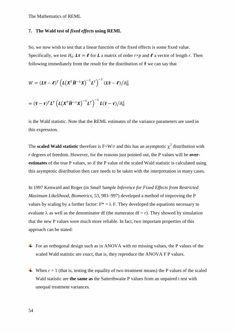
7. The Wald test of fixed effects using REML
So, we now wish to test that a linear function of the fixed effects is some fixed value.
Specifically, we test for a matrix of order r×p and a vector of length r. Then
following immediately from the result for the distribution of we can say that
( ) ( ( )
)
( ) ⁄
( ) ( ( )
)
( ) ⁄
is the Wald statistic. Note that the REML estimates of the variance parameters are used in
this expression.
The scaled Wald statistic therefore is F=W/r and this has an asymptotic 2 distribution with
r degrees of freedom. However, for the reasons just pointed out, the P values will be over-
estimates of the true P values, so if the P value of the scaled Wald statistic is calculated using
this asymptotic distribution then care needs to be taken with the interpretation in many cases.
In 1997 Kenward and Roger (in Small Sample Inference for Fixed Effects from Restricted
Maximum Likelihood, Biometrics, 53, 983–997) developed a method of improving the P
values by scaling by a further factor: F* = F. They developed the equations necessary to
evaluate as well as the denominator df (the numerator df = r). They showed by simulation
that the new P values were much more reliable. In fact, two important properties of this
approach can be stated:
For an orthogonal design such as in ANOVA with no missing values, the P values of the
scaled Wald statistic are exact, that is, they reproduce the ANOVA F P values.
When r = 1 (that is, testing the equality of two treatment means) the P values of the scaled
Wald statistic are the same as the Satterthwaite P values from an unpaired t test with
unequal treatment variances.
The Mathematics of REML
55
This implementation is now the default in GenStat. The equations can be very intensive, and
occasionally fail to solve, in which case GenStat resorts to P values obtained from the 2
distribution.
8. Testing the random effects
Random effects are assumed normally distributed, and hence this section addresses the way
to compare the LMM under one set of assumptions about the parameters in the variance
model with the LMM resulting in applying the values assumed under the hull hypothesis.
Note that this method therefore only applies
when models are nested, and
the same fixed parameters are in both models.
An examples of nested models is the sequence AR2 compared with AR1 and then with an
uncorrelated random effect. At time t:
yt = mean + a1 yt-1 + a2 yt-2 + error (AR2)
yt = mean + a1 yt-1 + error (AR1, obtained by testing a2 = 0)
yt = mean + error (uncorrelated, obtained by testing a1 = 0)
An example of models which are not nested is a comparison between a random variate
assumed to have an equi-correlated structure versus one with an AR1 structure. Both have
one correlation parameter and the same deviance degrees of freedom.
Deviance is defined as -2×logLikelihood where the logLikelihood is evaluated in terms of the
REML parameter estimates. Generally the constant in the logLikelihood is dropped because
the deviance is generally used only when differencing.
So, to test a subset of the variance parameters, start with the full model and obtain a reduced
model by evaluating the full model using the null hypothesis values of the variance
parameters. Then
Change in Deviance = Deviance for reduced model – Deviance for the full model
which is asymptotically with df = change in deviance df.
The Mathematics of REML
56
For example, for a model with a single random block variance and an error variance with 12
data values from 4 blocks and 3 treatments per block:
Deviance including the random block effect = 34.49 with 7 df (the FULL model)
Deviance excluding the random block effect = 51.38 with 8 df (the REDUCED model)
Change in deviance = 51.38 – 34.49 = 16.89 with 8 – 7 = 1 df which is highly significant
(P<0.001).
For models that are not nested GenStat offers two statistics, the Akaike Information
Coefficient (AIC) and the Schwarz Information Coefficient (SIC).
Let k be the number of variance parameters in the model. Then
AIC = Deviance + 2 k
There is no test value to compare this to. One proposal is to evaluate exp[(AIC1-AIC2)/2],
where AIC1 is the smaller and AIC2 the larger from the two models. This ratio can be thought
of as the probability that the second model minimises any information loss.
The Schwarz Information Coefficient is similar,
AIC = Deviance + ln(n) k
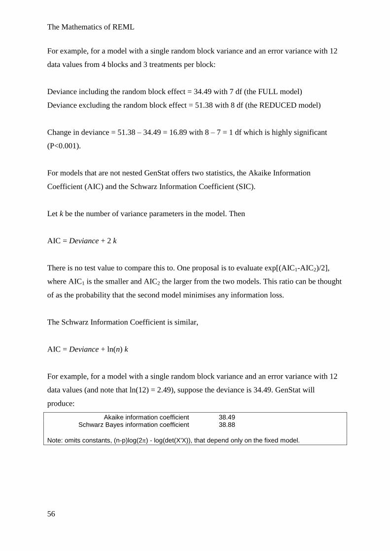
For example, for a model with a single random block variance and an error variance with 12
data values (and note that ln(12) = 2.49), suppose the deviance is 34.49. GenStat will
produce:
Akaike information coefficient 38.49 Schwarz Bayes information coefficient 38.88
Note: omits constants, (n-p)log(2) - log(det(X'X)), that depend only on the fixed model.
The Mathematics of REML
57
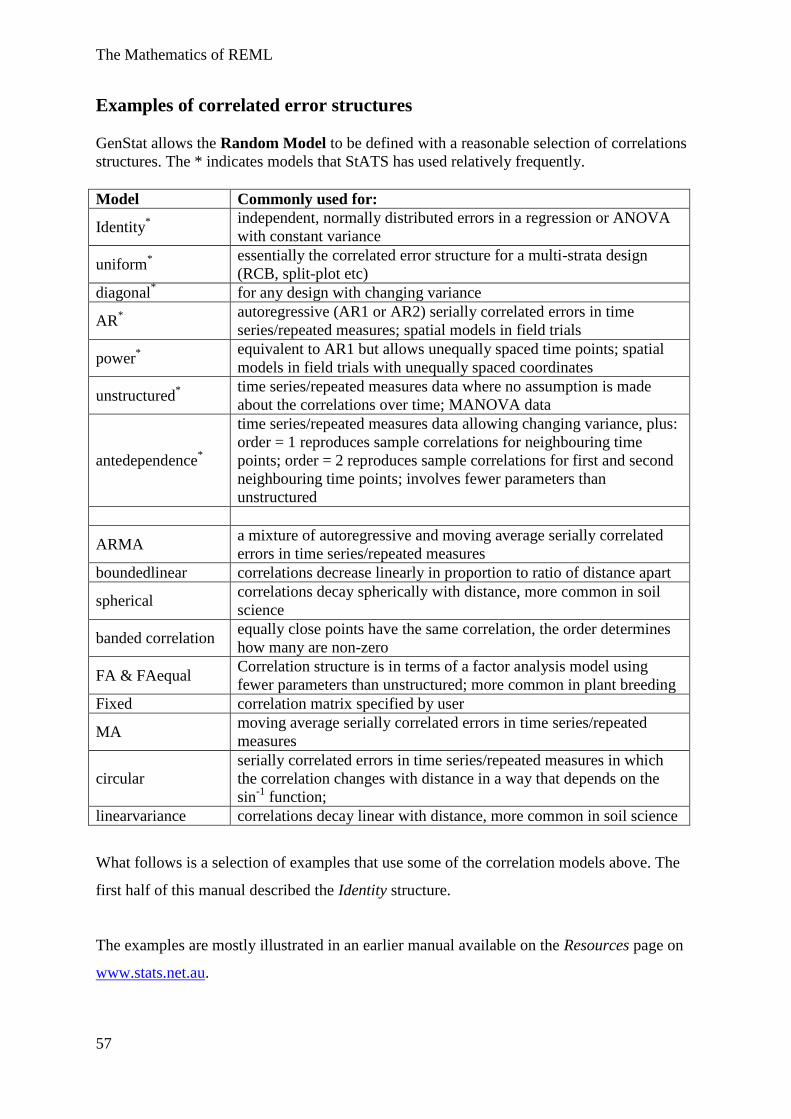
Examples of correlated error structures
GenStat allows the Random Model to be defined with a reasonable selection of correlations
structures. The * indicates models that StATS has used relatively frequently.
Model Commonly used for:
Identity*
independent, normally distributed errors in a regression or ANOVA
with constant variance
uniform*
essentially the correlated error structure for a multi-strata design
(RCB, split-plot etc)
diagonal* for any design with changing variance
AR*
autoregressive (AR1 or AR2) serially correlated errors in time
series/repeated measures; spatial models in field trials
power*
equivalent to AR1 but allows unequally spaced time points; spatial
models in field trials with unequally spaced coordinates
unstructured*
time series/repeated measures data where no assumption is made
about the correlations over time; MANOVA data
antedependence*
time series/repeated measures data allowing changing variance, plus:
order = 1 reproduces sample correlations for neighbouring time
points; order = 2 reproduces sample correlations for first and second
neighbouring time points; involves fewer parameters than
unstructured
ARMA a mixture of autoregressive and moving average serially correlated
errors in time series/repeated measures
boundedlinear correlations decrease linearly in proportion to ratio of distance apart
spherical correlations decay spherically with distance, more common in soil
science
banded correlation equally close points have the same correlation, the order determines
how many are non-zero
FA & FAequal Correlation structure is in terms of a factor analysis model using
fewer parameters than unstructured; more common in plant breeding
Fixed correlation matrix specified by user
MA moving average serially correlated errors in time series/repeated
measures
circular
serially correlated errors in time series/repeated measures in which
the correlation changes with distance in a way that depends on the
sin-1
function;
linearvariance correlations decay linear with distance, more common in soil science
What follows is a selection of examples that use some of the correlation models above. The
first half of this manual described the Identity structure.
The examples are mostly illustrated in an earlier manual available on the Resources page on
www.stats.net.au.
The Mathematics of REML
58
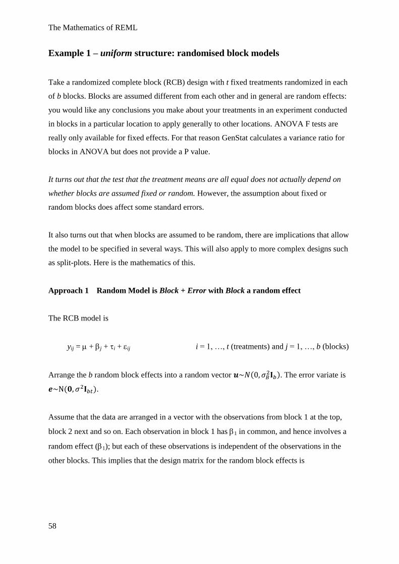
Example 1 – uniform structure: randomised block models
Take a randomized complete block (RCB) design with t fixed treatments randomized in each
of b blocks. Blocks are assumed different from each other and in general are random effects:
you would like any conclusions you make about your treatments in an experiment conducted
in blocks in a particular location to apply generally to other locations. ANOVA F tests are
really only available for fixed effects. For that reason GenStat calculates a variance ratio for
blocks in ANOVA but does not provide a P value.
It turns out that the test that the treatment means are all equal does not actually depend on
whether blocks are assumed fixed or random. However, the assumption about fixed or
random blocks does affect some standard errors.
It also turns out that when blocks are assumed to be random, there are implications that allow
the model to be specified in several ways. This will also apply to more complex designs such
as split-plots. Here is the mathematics of this.
Approach 1 Random Model is Block + Error with Block a random effect
The RCB model is
yij = + j + i + ij i = 1, …, t (treatments) and j = 1, …, b (blocks)
Arrange the b random block effects into a random vector ( ). The error variate is
( ).
Assume that the data are arranged in a vector with the observations from block 1 at the top,
block 2 next and so on. Each observation in block 1 has 1 in common, and hence involves a
random effect (1); but each of these observations is independent of the observations in the
other blocks. This implies that the design matrix for the random block effects is
The Mathematics of REML
59
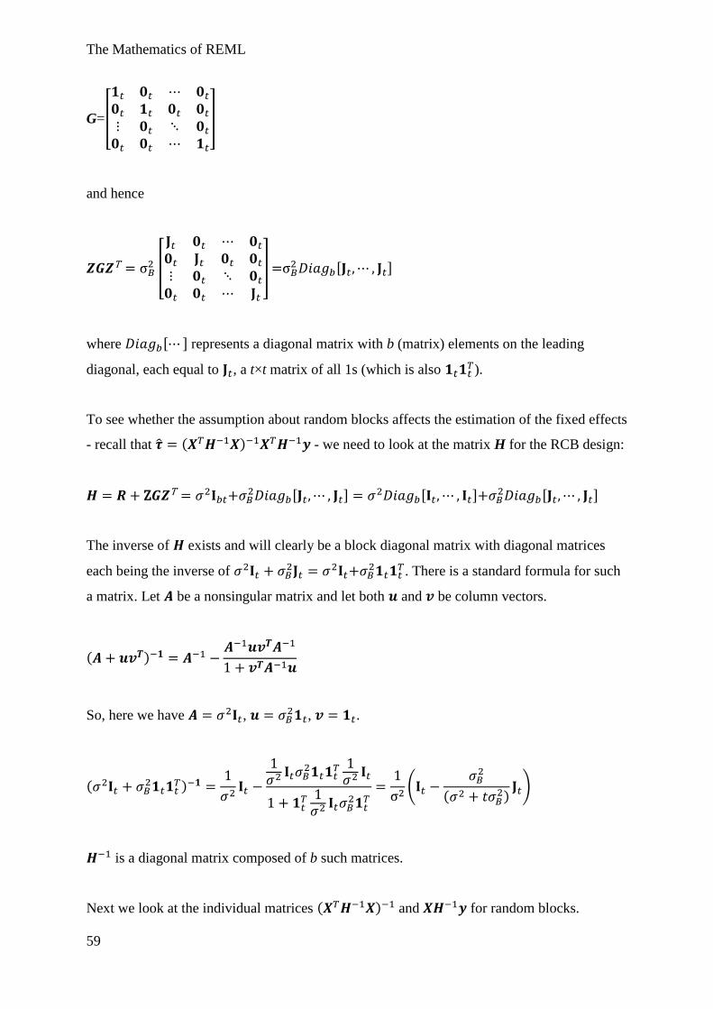
G=[
]
and hence
[
] [ ]
where [ ] represents a diagonal matrix with b (matrix) elements on the leading
diagonal, each equal to , a t×t matrix of all 1s (which is also ).
To see whether the assumption about random blocks affects the estimation of the fixed effects
- recall that ( ) - we need to look at the matrix H for the RCB design:
[ ] [ ]
[ ]
The inverse of exists and will clearly be a block diagonal matrix with diagonal matrices
each being the inverse of
. There is a standard formula for such
a matrix. Let be a nonsingular matrix and let both and be column vectors.
( )
So, here we have , , .
(
)
(
( )
)
is a diagonal matrix composed of b such matrices.
Next we look at the individual matrices ( ) and for random blocks.
The Mathematics of REML
60
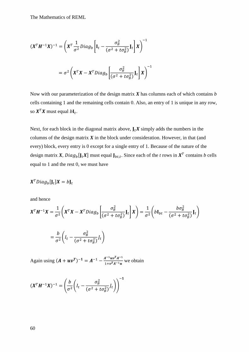
( ) (
[
( )
] )
( [
( )
] )
Now with our parameterization of the design matrix X has columns each of which contains b
cells containing 1 and the remaining cells contain 0. Also, an entry of 1 is unique in any row,
so must equal .
Next, for each block in the diagonal matrix above, simply adds the numbers in the
columns of the design matrix X in the block under consideration. However, in that (and
every) block, every entry is 0 except for a single entry of 1. Because of the nature of the
design matrix X, [ ] must equal . Since each of the t rows in contains b cells
equal to 1 and the rest 0, we must have
[ ]
and hence
( [
( )
] )
(
( )
)
(
( )
)
Again using ( )
we obtain
( ) (
(
( )
))
The Mathematics of REML
61
(
( )
( )
)
(
)
This is a matrix with diagonal elements equal to ⁄ ⁄ and off-diagonal elements
⁄ .
The last term to evaluate is partly resolved since we know : it consists of t rows, each
having b cells equal to ( (
)⁄ ) ⁄ and t(b-1) cells all equal to
(
)⁄ ⁄ . The positions of these cells are dictated by the design matrix X,
however when is post-multiplied by y, the ith
row results in the ith
treatment mean
as well as the grand mean . We need to introduce the vector of data means which we’ll
denote as ( ). Then
( )
Combining the two terms and replacing terms like by leads to
( )
(
)(
( )
)
(
( )
( )
)
((
)
( )
)
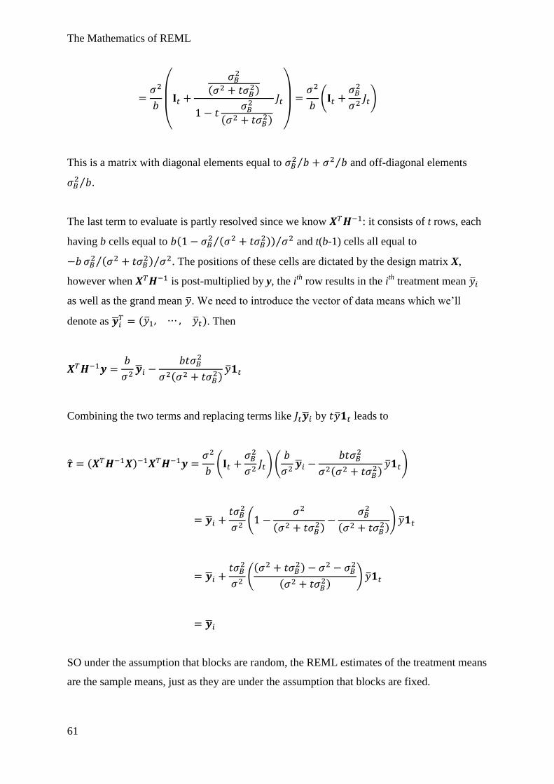
SO under the assumption that blocks are random, the REML estimates of the treatment means
are the sample means, just as they are under the assumption that blocks are fixed.
The Mathematics of REML
62
However the standard errors of the means are larger under the random blocks model
compared to the fixed blocks model. This is not surprising, since in order to be applicable to
other blocks one needs to be more cautious in estimating individual treatment means.
Nevertheless, the standard errors of differences of means are the same under both
assumptions.
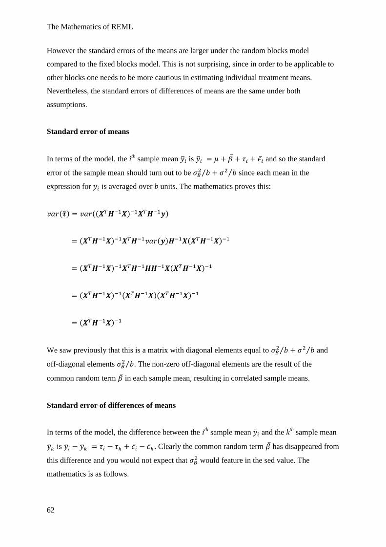
Standard error of means
In terms of the model, the ith
sample mean is and so the standard
error of the sample mean should turn out to be ⁄ ⁄ since each mean in the
expression for is averaged over b units. The mathematics proves this:
( ) (( ) )
( ) ( ) ( )
( ) ( )
( ) ( )( )
( )
We saw previously that this is a matrix with diagonal elements equal to ⁄ ⁄ and
off-diagonal elements ⁄ . The non-zero off-diagonal elements are the result of the
common random term in each sample mean, resulting in correlated sample means.
Standard error of differences of means
In terms of the model, the difference between the ith
sample mean and the kth
sample mean
is . Clearly the common random term has disappeared from
this difference and you would not expect that would feature in the sed value. The
mathematics is as follows.
The Mathematics of REML
63
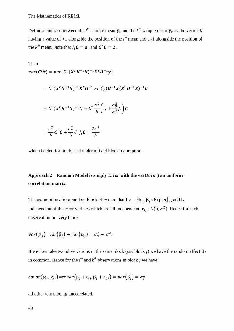
Define a contrast between the ith
sample mean and the kth
sample mean as the vector
having a value of +1 alongside the position of the ith
mean and a -1 alongside the position of
the kth
mean. Note that and .
Then
( ) ( ( ) )
( ) ( ) ( )
( )
(
)
which is identical to the sed under a fixed block assumption.
Approach 2 Random Model is simply Error with the var(Error) an uniform
correlation matrix.
The assumptions for a random block effect are that for each j, ( ), and is
independent of the error variates which are all independent, ( ). Hence for each
observation in every block,
( ) ( ) ( ) .
If we now take two observations in the same block (say block j) we have the random effect
in common. Hence for the ith
and kth
observations in block j we have
( ) ( ) ( )
all other terms being uncorrelated.
The Mathematics of REML
64
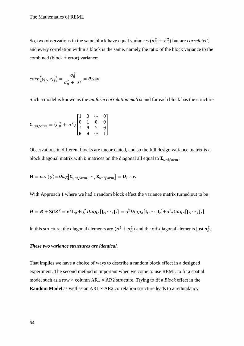
So, two observations in the same block have equal variances ( ) but are correlated,
and every correlation within a block is the same, namely the ratio of the block variance to the
combined (block + error) variance:
( )
Such a model is known as the uniform correlation matrix and for each block has the structure
( ) [
]
Observations in different blocks are uncorrelated, and so the full design variance matrix is a
block diagonal matrix with b matrices on the diagonal all equal to :
( ) [ ]
With Approach 1 where we had a random block effect the variance matrix turned out to be
[ ] [ ]
[ ]
In this structure, the diagonal elements are ( ) and the off-diagonal elements just
.
These two variance structures are identical.
That implies we have a choice of ways to describe a random block effect in a designed
experiment. The second method is important when we come to use REML to fit a spatial
model such as a row × column AR1 × AR2 structure. Trying to fit a Block effect in the
Random Model as well as an AR1 × AR2 correlation structure leads to a redundancy.
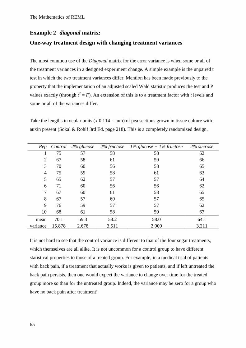
The Mathematics of REML
65
Example 2 diagonal matrix:
One-way treatment design with changing treatment variances
The most common use of the Diagonal matrix for the error variance is when some or all of
the treatment variances in a designed experiment change. A simple example is the unpaired t
test in which the two treatment variances differ. Mention has been made previously to the
property that the implementation of an adjusted scaled Wald statistic produces the test and P
values exactly (through t2 = F). An extension of this is to a treatment factor with t levels and
some or all of the variances differ.
Take the lengths in ocular units (x 0.114 = mm) of pea sections grown in tissue culture with
auxin present (Sokal & Rohlf 3rd Ed. page 218). This is a completely randomized design.
Rep Control 2% glucose 2% fructose 1% glucose + 1% fructose 2% sucrose
1 75 57 58 58 62
2 67 58 61 59 66
3 70 60 56 58 65
4 75 59 58 61 63
5 65 62 57 57 64
6 71 60 56 56 62
7 67 60 61 58 65
8 67 57 60 57 65
9 76 59 57 57 62
10 68 61 58 59 67
mean 70.1 59.3 58.2 58.0 64.1
variance 15.878 2.678 3.511 2.000 3.211
It is not hard to see that the control variance is different to that of the four sugar treatments,
which themselves are all alike. It is not uncommon for a control group to have different
statistical properties to those of a treated group. For example, in a medical trial of patients
with back pain, if a treatment that actually works is given to patients, and if left untreated the
back pain persists, then one would expect the variance to change over time for the treated
group more so than for the untreated group. Indeed, the variance may be zero for a group who
have no back pain after treatment!
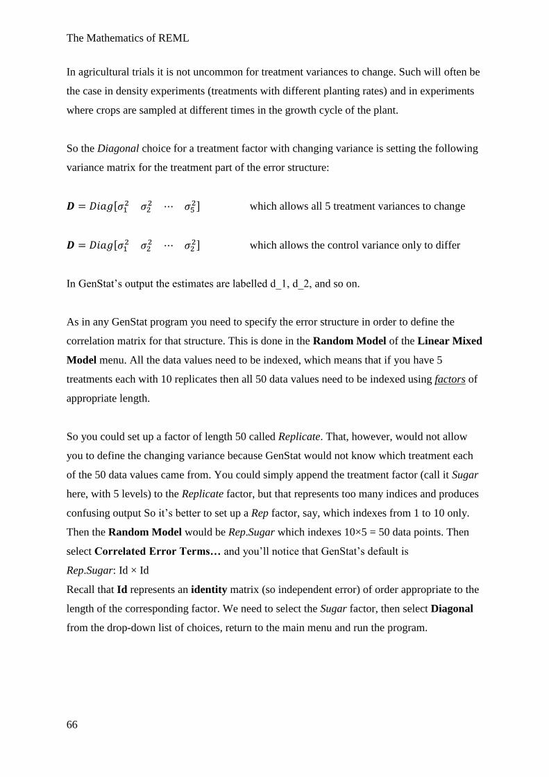
The Mathematics of REML
66
In agricultural trials it is not uncommon for treatment variances to change. Such will often be
the case in density experiments (treatments with different planting rates) and in experiments
where crops are sampled at different times in the growth cycle of the plant.
So the Diagonal choice for a treatment factor with changing variance is setting the following
variance matrix for the treatment part of the error structure:
[
] which allows all 5 treatment variances to change
[
] which allows the control variance only to differ
In GenStat’s output the estimates are labelled d_1, d_2, and so on.
As in any GenStat program you need to specify the error structure in order to define the
correlation matrix for that structure. This is done in the Random Model of the Linear Mixed
Model menu. All the data values need to be indexed, which means that if you have 5
treatments each with 10 replicates then all 50 data values need to be indexed using factors of
appropriate length.
So you could set up a factor of length 50 called Replicate. That, however, would not allow
you to define the changing variance because GenStat would not know which treatment each
of the 50 data values came from. You could simply append the treatment factor (call it Sugar
here, with 5 levels) to the Replicate factor, but that represents too many indices and produces
confusing output So it’s better to set up a Rep factor, say, which indexes from 1 to 10 only.
Then the Random Model would be Rep.Sugar which indexes 10×5 = 50 data points. Then
select Correlated Error Terms… and you’ll notice that GenStat’s default is
Rep.Sugar: Id × Id
Recall that Id represents an identity matrix (so independent error) of order appropriate to the
length of the corresponding factor. We need to select the Sugar factor, then select Diagonal
from the drop-down list of choices, return to the main menu and run the program.
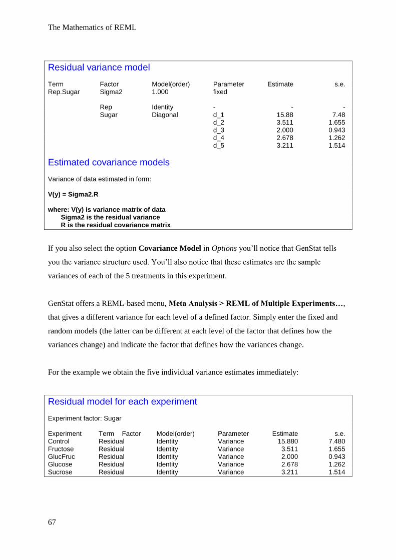
The Mathematics of REML
67
Residual variance model Term Factor Model(order) Parameter Estimate s.e. Rep.Sugar Sigma2 1.000 fixed Rep Identity - - - Sugar Diagonal d_1 15.88 7.48 d_2 3.511 1.655 d_3 2.000 0.943 d_4 2.678 1.262 d_5 3.211 1.514
Estimated covariance models
Variance of data estimated in form: V(y) = Sigma2.R where: V(y) is variance matrix of data Sigma2 is the residual variance R is the residual covariance matrix
If you also select the option Covariance Model in Options you’ll notice that GenStat tells
you the variance structure used. You’ll also notice that these estimates are the sample
variances of each of the 5 treatments in this experiment.
GenStat offers a REML-based menu, Meta Analysis > REML of Multiple Experiments…,
that gives a different variance for each level of a defined factor. Simply enter the fixed and
random models (the latter can be different at each level of the factor that defines how the
variances change) and indicate the factor that defines how the variances change.
For the example we obtain the five individual variance estimates immediately:
Residual model for each experiment Experiment factor: Sugar Experiment Term Factor Model(order) Parameter Estimate s.e. Control Residual Identity Variance 15.880 7.480 Fructose Residual Identity Variance 3.511 1.655 GlucFruc Residual Identity Variance 2.000 0.943 Glucose Residual Identity Variance 2.678 1.262 Sucrose Residual Identity Variance 3.211 1.514
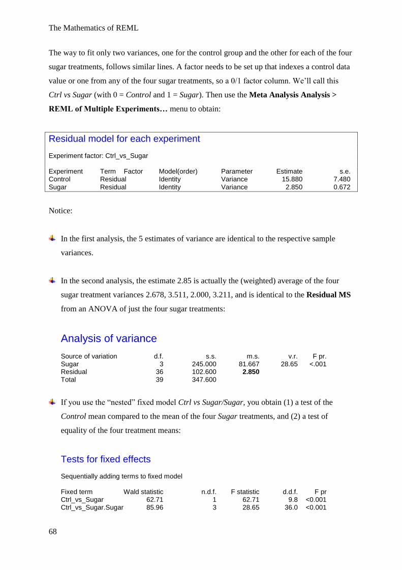
The Mathematics of REML
68
The way to fit only two variances, one for the control group and the other for each of the four
sugar treatments, follows similar lines. A factor needs to be set up that indexes a control data
value or one from any of the four sugar treatments, so a 0/1 factor column. We’ll call this
Ctrl vs Sugar (with 0 = Control and 1 = Sugar). Then use the Meta Analysis Analysis >
REML of Multiple Experiments… menu to obtain:
Residual model for each experiment Experiment factor: Ctrl_vs_Sugar Experiment Term Factor Model(order) Parameter Estimate s.e. Control Residual Identity Variance 15.880 7.480 Sugar Residual Identity Variance 2.850 0.672
Notice:
In the first analysis, the 5 estimates of variance are identical to the respective sample
variances.
In the second analysis, the estimate 2.85 is actually the (weighted) average of the four
sugar treatment variances 2.678, 3.511, 2.000, 3.211, and is identical to the Residual MS
from an ANOVA of just the four sugar treatments:
Analysis of variance
Source of variation d.f. s.s. m.s. v.r. F pr. Sugar 3 245.000 81.667 28.65 <.001 Residual 36 102.600 2.850 Total 39 347.600
If you use the “nested” fixed model Ctrl vs Sugar/Sugar, you obtain (1) a test of the
Control mean compared to the mean of the four Sugar treatments, and (2) a test of
equality of the four treatment means:
Tests for fixed effects
Sequentially adding terms to fixed model Fixed term Wald statistic n.d.f. F statistic d.d.f. F pr Ctrl_vs_Sugar 62.71 1 62.71 9.8 <0.001 Ctrl_vs_Sugar.Sugar 85.96 3 28.65 36.0 <0.001
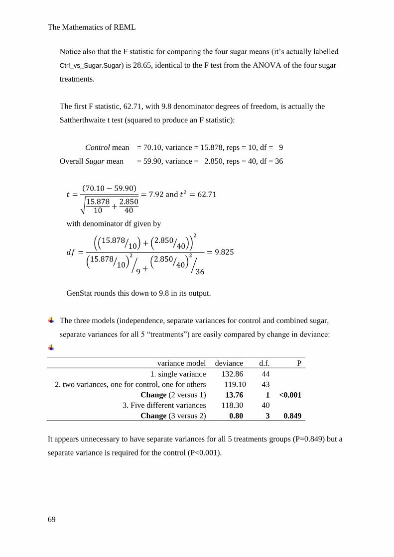
The Mathematics of REML
69
Notice also that the F statistic for comparing the four sugar means (it’s actually labelled
Ctrl_vs_Sugar.Sugar) is 28.65, identical to the F test from the ANOVA of the four sugar
treatments.
The first F statistic, 62.71, with 9.8 denominator degrees of freedom, is actually the
Sattherthwaite t test (squared to produce an F statistic):
Control mean = 70.10, variance = 15.878, reps = 10, df = 9
Overall Sugar mean = 59.90, variance = 2.850, reps = 40, df = 36
( )
√
with denominator df given by
(( ⁄ ) ( ⁄ ))
( ⁄ )
⁄
( ⁄ )
⁄
GenStat rounds this down to 9.8 in its output.
The three models (independence, separate variances for control and combined sugar,
separate variances for all 5 “treatments”) are easily compared by change in deviance:
variance model deviance d.f. P
1. single variance 132.86 44
2. two variances, one for control, one for others 119.10 43
Change (2 versus 1) 13.76 1 <0.001
3. Five different variances 118.30 40
Change (3 versus 2) 0.80 3 0.849
It appears unnecessary to have separate variances for all 5 treatments groups (P=0.849) but a
separate variance is required for the control (P<0.001).
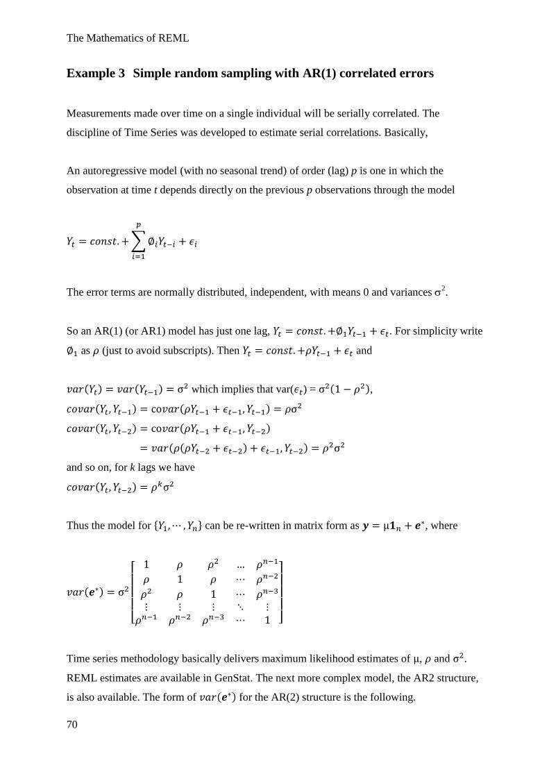
The Mathematics of REML
70
Example 3 Simple random sampling with AR(1) correlated errors
Measurements made over time on a single individual will be serially correlated. The
discipline of Time Series was developed to estimate serial correlations. Basically,
An autoregressive model (with no seasonal trend) of order (lag) p is one in which the
observation at time t depends directly on the previous p observations through the model
∑
The error terms are normally distributed, independent, with means 0 and variances 2.
So an AR(1) (or AR1) model has just one lag, . For simplicity write
as (just to avoid subscripts). Then and
( ) ( ) which implies that var( ) = ( ),
( ) ( )
( ) ( )
( ( ) )
and so on, for k lags we have
( )
Thus the model for can be re-written in matrix form as , where
( )
[
]
Time series methodology basically delivers maximum likelihood estimates of , and .
REML estimates are available in GenStat. The next more complex model, the AR2 structure,
is also available. The form of ( ) for the AR(2) structure is the following.
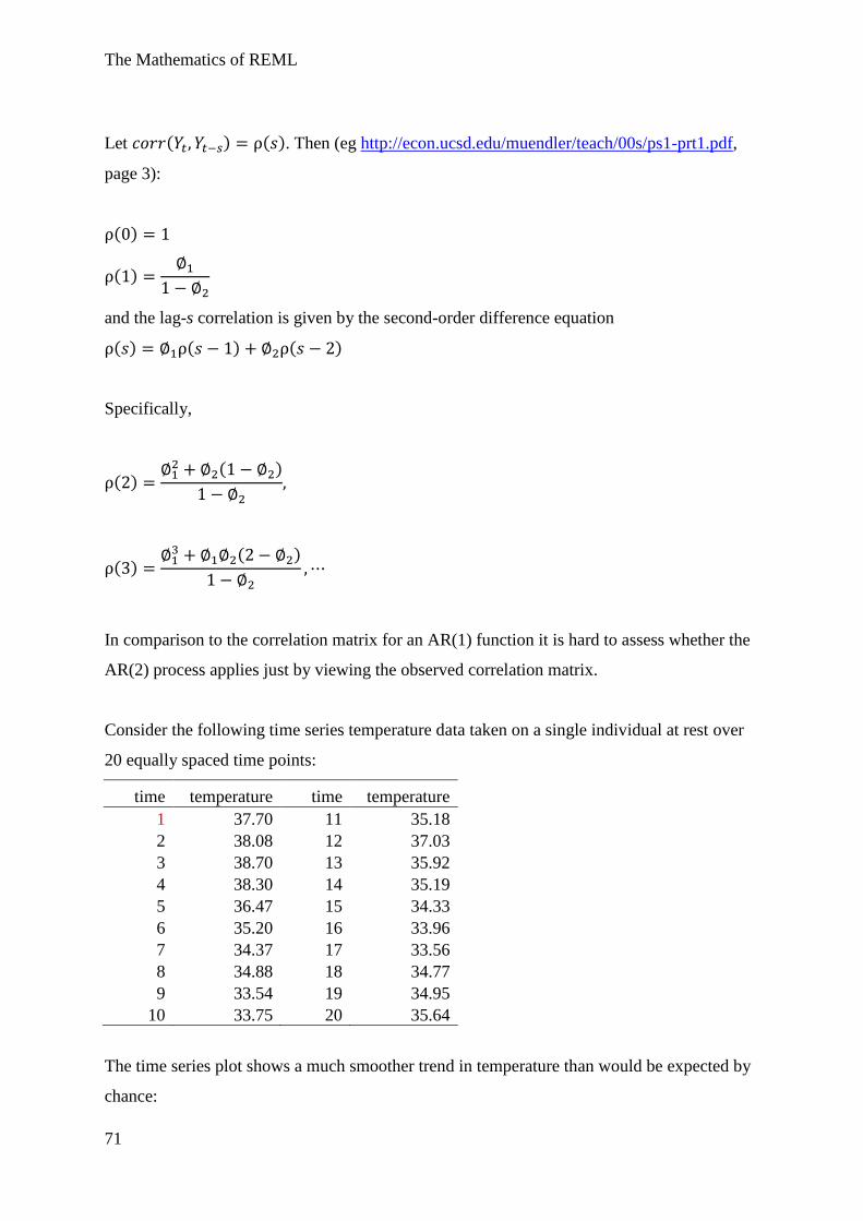
The Mathematics of REML
71
Let ( ) ( ). Then (eg http://econ.ucsd.edu/muendler/teach/00s/ps1-prt1.pdf,
page 3):
( )
( )
and the lag-s correlation is given by the second-order difference equation
( ) ( ) ( )
Specifically,
( )
( )
( )
( )
In comparison to the correlation matrix for an AR(1) function it is hard to assess whether the
AR(2) process applies just by viewing the observed correlation matrix.
Consider the following time series temperature data taken on a single individual at rest over
20 equally spaced time points:
time temperature time temperature
1 37.70 11 35.18
2 38.08 12 37.03
3 38.70 13 35.92
4 38.30 14 35.19
5 36.47 15 34.33
6 35.20 16 33.96
7 34.37 17 33.56
8 34.88 18 34.77
9 33.54 19 34.95
10 33.75 20 35.64
The time series plot shows a much smoother trend in temperature than would be expected by
chance:
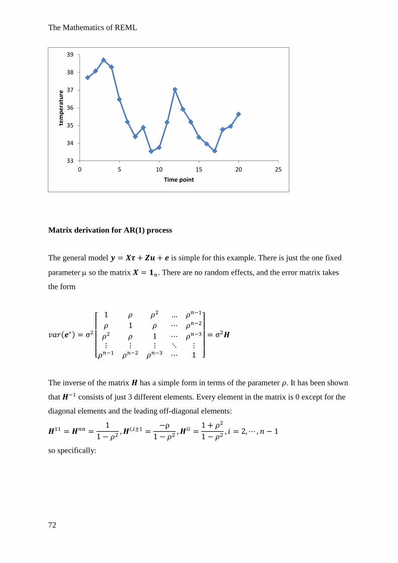
The Mathematics of REML
72
Matrix derivation for AR(1) process
The general model is simple for this example. There is just the one fixed
parameter so the matrix . There are no random effects, and the error matrix takes
the form
( )
[
]
The inverse of the matrix has a simple form in terms of the parameter . It has been shown
that consists of just 3 different elements. Every element in the matrix is 0 except for the
diagonal elements and the leading off-diagonal elements:
so specifically:
33
34
35
36
37
38
39
0 5 10 15 20 25
tem
pe
ratu
re
Time point
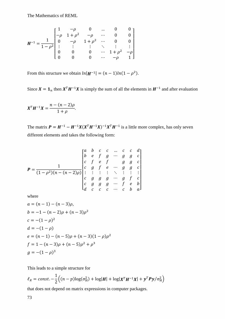
The Mathematics of REML
73
[
]
From this structure we obtain | | ( ) ( ).
Since then is simply the sum of all the elements in and after evaluation
( )
The matrix ( ) is a little more complex, has only seven
different elements and takes the following form:
( )( ( ) )
[
]
where
( ) ( ) ,
( ) ( )
( )
( )
( ) ( ) ( )( )
( ) ( )
( )
This leads to a simple structure for
(( ) (
) | | | | ⁄ )
that does not depend on matrix expressions in computer packages.
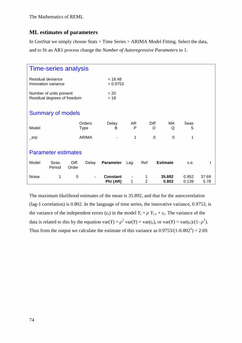
The Mathematics of REML
74
ML estimates of parameters
In GenStat we simply choose Stats > Time Series > ARIMA Model Fitting. Select the data,
and to fit an AR1 process change the Number of Autoregressive Parameters to 1.
Time-series analysis
Residual deviance = 18.48 Innovation variance = 0.9753 Number of units present = 20 Residual degrees of freedom = 18
Summary of models
Orders: Delay AR Diff MA Seas Model Type B P D Q S _erp ARIMA - 1 0 0 1
Parameter estimates
Model Seas. Diff. Delay Parameter Lag Ref Estimate s.e. t Period Order Noise 1 0 - Constant - 1 35.892 0.952 37.69 Phi (AR) 1 2 0.802 0.139 5.78
The maximum likelihood estimates of the mean is 35.892, and that for the autocorrelation
(lag-1 correlation) is 0.802. In the language of time series, the innovative variance, 0.9753, is
the variance of the independent errors (t) in the model Yt = Yt-1 + t. The variance of the
data is related to this by the equation var(Y) = var(Y) + var(t), or var(Y) = var(t)/(1-
).
Thus from the output we calculate the estimate of this variance as 0.9753/(1-0.8022) = 2.69.
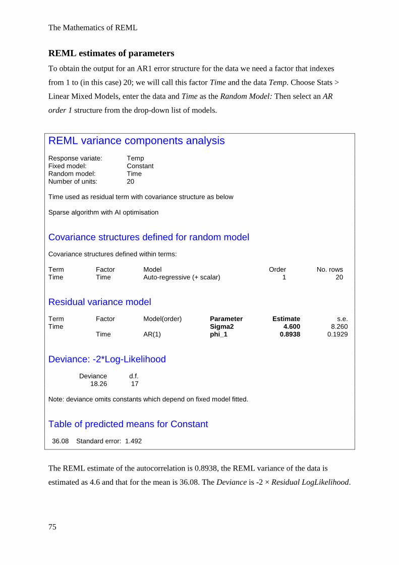
The Mathematics of REML
75
REML estimates of parameters
To obtain the output for an AR1 error structure for the data we need a factor that indexes
from 1 to (in this case) 20; we will call this factor Time and the data Temp. Choose Stats >
Linear Mixed Models, enter the data and Time as the Random Model: Then select an AR
order 1 structure from the drop-down list of models.
REML variance components analysis
Response variate: Temp Fixed model: Constant Random model: Time Number of units: 20 Time used as residual term with covariance structure as below Sparse algorithm with AI optimisation
Covariance structures defined for random model Covariance structures defined within terms: Term Factor Model Order No. rows Time Time Auto-regressive (+ scalar) 1 20
Residual variance model Term Factor Model(order) Parameter Estimate s.e. Time Sigma2 4.600 8.260 Time AR(1) phi_1 0.8938 0.1929
Deviance: -2*Log-Likelihood
Deviance d.f. 18.26 17 Note: deviance omits constants which depend on fixed model fitted.
Table of predicted means for Constant 36.08 Standard error: 1.492
The REML estimate of the autocorrelation is 0.8938, the REML variance of the data is
estimated as 4.6 and that for the mean is 36.08. The Deviance is -2 × Residual LogLikelihood.
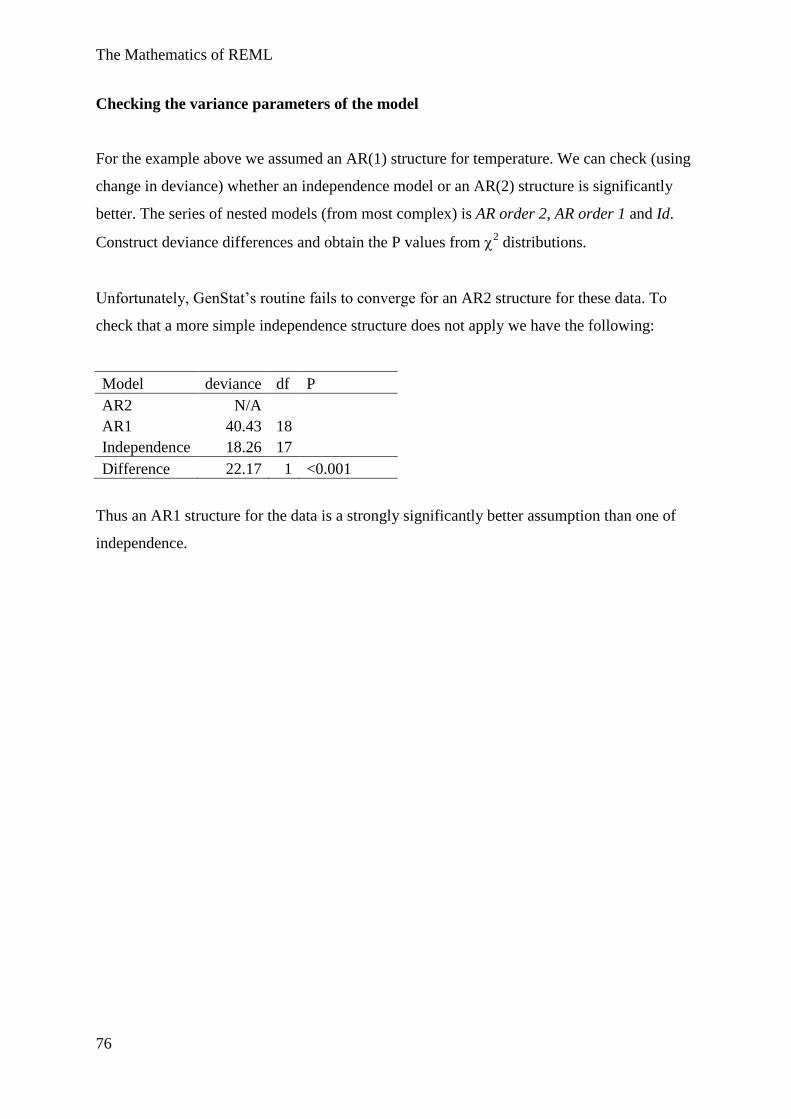
The Mathematics of REML
76
Checking the variance parameters of the model
For the example above we assumed an AR(1) structure for temperature. We can check (using
change in deviance) whether an independence model or an AR(2) structure is significantly
better. The series of nested models (from most complex) is AR order 2, AR order 1 and Id.
Construct deviance differences and obtain the P values from 2 distributions.
Unfortunately, GenStat’s routine fails to converge for an AR2 structure for these data. To
check that a more simple independence structure does not apply we have the following:
Model deviance df P
AR2 N/A
AR1 40.43 18
Independence 18.26 17
Difference 22.17 1 <0.001
Thus an AR1 structure for the data is a strongly significantly better assumption than one of
independence.
The Mathematics of REML
77
Example 4 Repeated measures data, unstructured/antedependence
structures
Often a researcher will measure the same experimental units over time. In pre-computer times
a standard split-plot analysis was used with time as the split factor. We have seen that such a
model implies that the data are uniformly correlated over time. This is not plausible for many
experimental situations: it is more likely that the correlation is stronger for observations taken
closer together than further apart. Models that are commonly used include AR1 and AR2
structures, unstructured and antedependence order 1 and order 2 structures.
One should also anticipate a variance that changes over time. For example, if measurements
are made on the growth of a single animal over the exponential phrase of growth, the
variance will most likely increase with time. On the other hand patients who undergo
treatment for back pain are likely to have a reduction in back pain, and if the treatment is
100% successful the variance at the end of treatment should be 0!
GenStat has a specialised menu for simple one-way blocked or unblocked designs that offer
the usual correlation models mentioned above as well as possible changing variance. To
demonstrate the range of models we will consider GenStat’s example “studying the effects of
preserving liquids on the enzyme content of dog hearts”. The variate measured was the
percentage of total enzyme in the heart, at one and two hourly intervals (hourly from 0 hours
to 6 hours, then at 8, 10 and 12 hours) during a twelve hour period following initial
preservation. There were two treatments labelled A and B each at two levels. Only 23 hearts
were used, 6 hearts for three treatment combinations and 5 hearts for the other. The design is
therefore unbalanced.
A1, B1 A1, B2 A1, B3 …
Time Heart 1 Heart 2 Heart 3 …
1 85.51 76.54 66.03 …
2 74.56 72.77 66.67 …
3 84.25 86.93 77.57 …
… … … … …
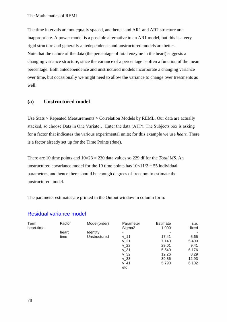
The Mathematics of REML
78
The time intervals are not equally spaced, and hence and AR1 and AR2 structure are
inappropriate. A power model is a possible alternative to an AR1 model, but this is a very
rigid structure and generally antedependence and unstructured models are better.
Note that the nature of the data (the percentage of total enzyme in the heart) suggests a
changing variance structure, since the variance of a percentage is often a function of the mean
percentage. Both antedependence and unstructured models incorporate a changing variance
over time, but occasionally we might need to allow the variance to change over treatments as
well.
(a) Unstructured model
Use Stats > Repeated Measurements > Correlation Models by REML. Our data are actually
stacked, so choose Data in One Variate… Enter the data (ATP). The Subjects box is asking
for a factor that indicates the various experimental units; for this example we use heart. There
is a factor already set up for the Time Points (time).
There are 10 time points and 10×23 = 230 data values so 229 df for the Total MS. An
unstructured covariance model for the 10 time points has 10×11/2 = 55 individual
parameters, and hence there should be enough degrees of freedom to estimate the
unstructured model.
The parameter estimates are printed in the Output window in column form:
Residual variance model Term Factor Model(order) Parameter Estimate s.e. heart.time Sigma2 1.000 fixed heart Identity - - - time Unstructured v_11 17.41 5.65 v_21 7.140 5.409 v_22 29.01 9.41 v_31 5.549 6.176 v_32 12.26 8.29 v_33 39.86 12.93 v_41 5.790 6.102 etc
The Mathematics of REML
79
Here v_11 represents the variance at time 1, v_22 the variance at time 2, and so on; v_21
represents the covariance at times 1 and 2, v_31 the covariance at times 1 and 3, and so on.
There is an Option to tick (Covariance Model) to have this printed in matrix form:
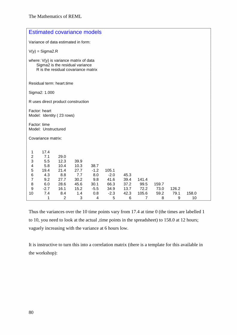
The Mathematics of REML
80
Estimated covariance models
Variance of data estimated in form: V(y) = Sigma2.R where: V(y) is variance matrix of data Sigma2 is the residual variance R is the residual covariance matrix Residual term: heart.time Sigma2: 1.000 R uses direct product construction Factor: heart Model: Identity ( 23 rows) Factor: time Model: Unstructured Covariance matrix: 1 17.4 2 7.1 29.0 3 5.5 12.3 39.9 4 5.8 10.4 10.3 38.7 5 19.4 21.4 27.7 -1.2 105.1 6 4.3 8.8 7.7 8.0 -2.0 45.3 7 9.2 27.7 30.2 9.8 41.6 39.4 141.4 8 6.0 28.6 45.6 30.1 66.3 37.2 99.5 159.7 9 -2.7 16.1 15.2 -5.5 34.9 13.7 72.2 73.0 126.2 10 7.4 8.4 1.4 0.8 -2.3 42.3 105.6 59.2 79.1 158.0 1 2 3 4 5 6 7 8 9 10
Thus the variances over the 10 time points vary from 17.4 at time 0 (the times are labelled 1
to 10, you need to look at the actual ,time points in the spreadsheet) to 158.0 at 12 hours;
vaguely increasing with the variance at 6 hours low.
It is instructive to turn this into a correlation matrix (there is a template for this available in
the workshop):
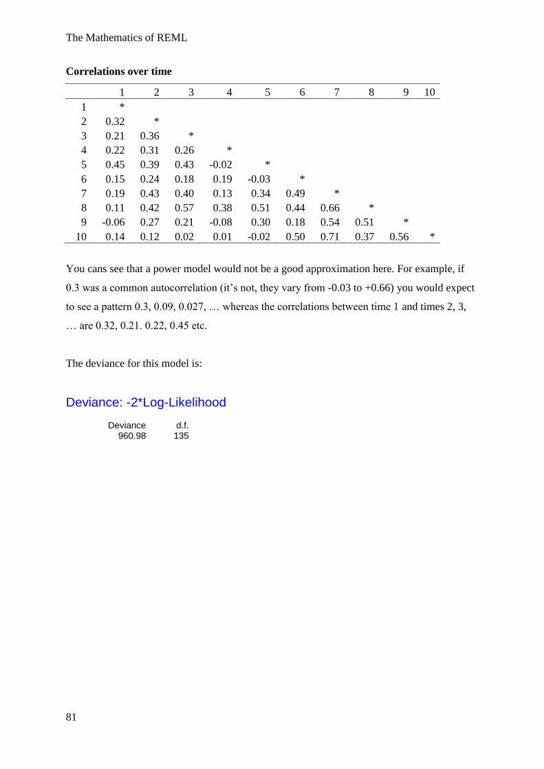
The Mathematics of REML
81
Correlations over time
1 2 3 4 5 6 7 8 9 10
1 *
2 0.32 *
3 0.21 0.36 *
4 0.22 0.31 0.26 *
5 0.45 0.39 0.43 -0.02 *
6 0.15 0.24 0.18 0.19 -0.03 *
7 0.19 0.43 0.40 0.13 0.34 0.49 *
8 0.11 0.42 0.57 0.38 0.51 0.44 0.66 *
9 -0.06 0.27 0.21 -0.08 0.30 0.18 0.54 0.51 *
10 0.14 0.12 0.02 0.01 -0.02 0.50 0.71 0.37 0.56 *
You cans see that a power model would not be a good approximation here. For example, if
0.3 was a common autocorrelation (it’s not, they vary from -0.03 to +0.66) you would expect
to see a pattern 0.3, 0.09, 0.027, … whereas the correlations between time 1 and times 2, 3,
… are 0.32, 0.21. 0.22, 0.45 etc.
The deviance for this model is:
Deviance: -2*Log-Likelihood
Deviance d.f. 960.98 135
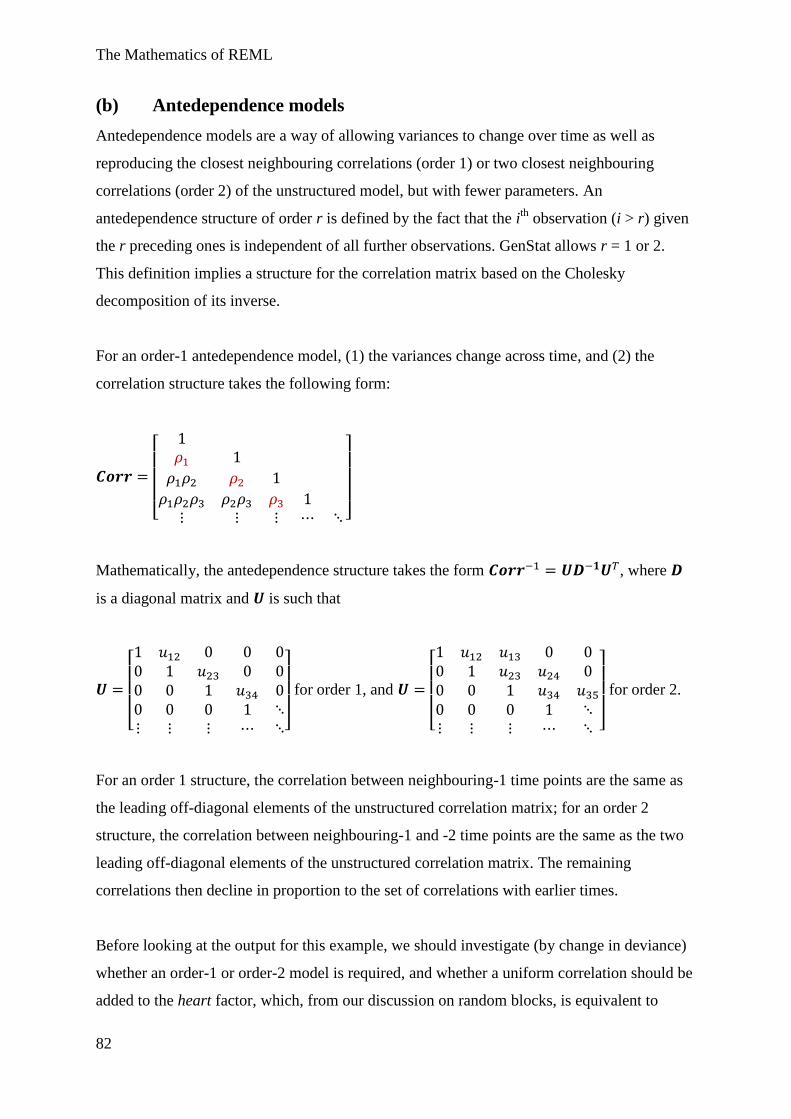
The Mathematics of REML
82
(b) Antedependence models
Antedependence models are a way of allowing variances to change over time as well as
reproducing the closest neighbouring correlations (order 1) or two closest neighbouring
correlations (order 2) of the unstructured model, but with fewer parameters. An
antedependence structure of order r is defined by the fact that the ith
observation (i > r) given
the r preceding ones is independent of all further observations. GenStat allows r = 1 or 2.
This definition implies a structure for the correlation matrix based on the Cholesky
decomposition of its inverse.
For an order-1 antedependence model, (1) the variances change across time, and (2) the
correlation structure takes the following form:
[
]
Mathematically, the antedependence structure takes the form , where
is a diagonal matrix and is such that
[ ]
for order 1, and
[
]
for order 2.
For an order 1 structure, the correlation between neighbouring-1 time points are the same as
the leading off-diagonal elements of the unstructured correlation matrix; for an order 2
structure, the correlation between neighbouring-1 and -2 time points are the same as the two
leading off-diagonal elements of the unstructured correlation matrix. The remaining
correlations then decline in proportion to the set of correlations with earlier times.
Before looking at the output for this example, we should investigate (by change in deviance)
whether an order-1 or order-2 model is required, and whether a uniform correlation should be
added to the heart factor, which, from our discussion on random blocks, is equivalent to
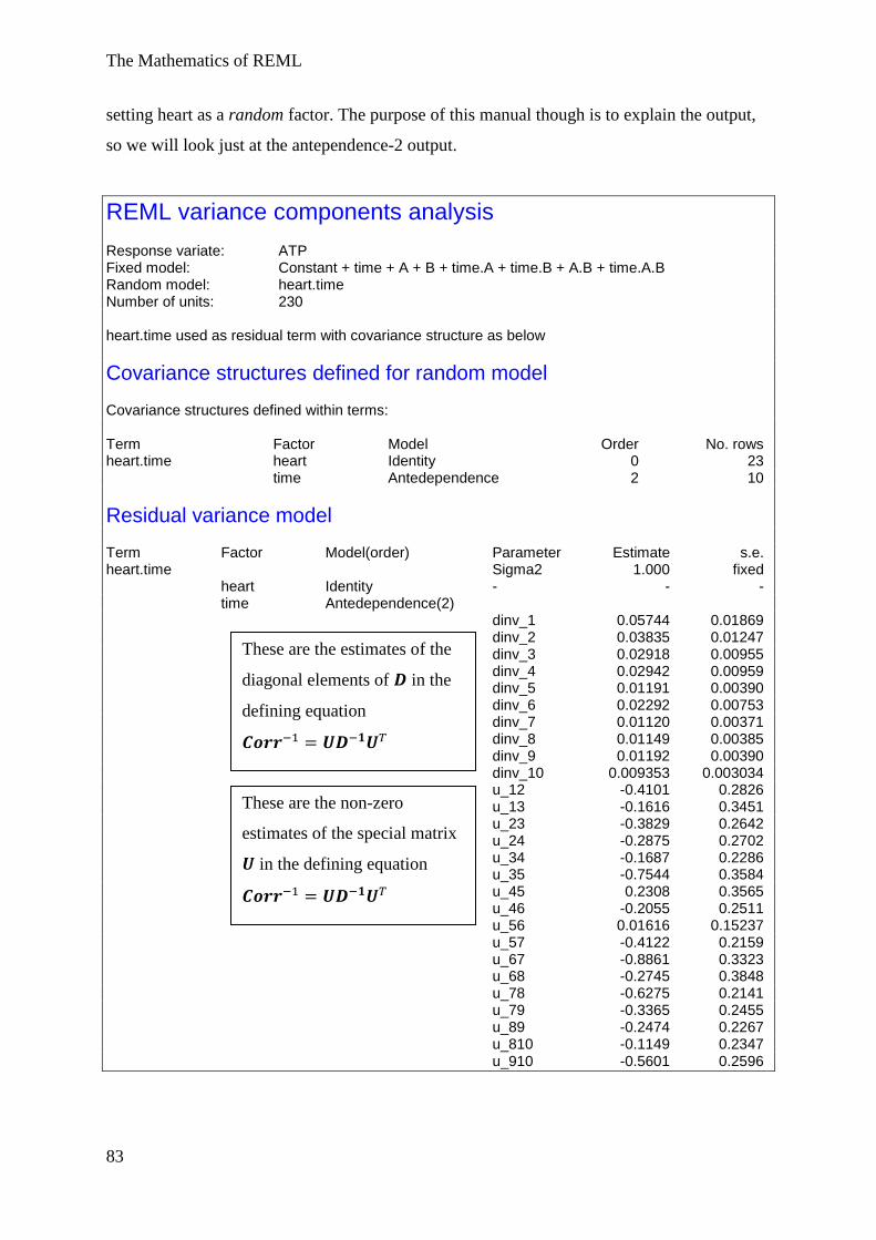
The Mathematics of REML
83
setting heart as a random factor. The purpose of this manual though is to explain the output,
so we will look just at the antependence-2 output.
REML variance components analysis
Response variate: ATP Fixed model: Constant + time + A + B + time.A + time.B + A.B + time.A.B Random model: heart.time Number of units: 230 heart.time used as residual term with covariance structure as below
Covariance structures defined for random model Covariance structures defined within terms: Term Factor Model Order No. rows heart.time heart Identity 0 23 time Antedependence 2 10
Residual variance model Term Factor Model(order) Parameter Estimate s.e. heart.time Sigma2 1.000 fixed heart Identity - - - time Antedependence(2) dinv_1 0.05744 0.01869 dinv_2 0.03835 0.01247 dinv_3 0.02918 0.00955 dinv_4 0.02942 0.00959 dinv_5 0.01191 0.00390 dinv_6 0.02292 0.00753 dinv_7 0.01120 0.00371 dinv_8 0.01149 0.00385 dinv_9 0.01192 0.00390 dinv_10 0.009353 0.003034 u_12 -0.4101 0.2826 u_13 -0.1616 0.3451 u_23 -0.3829 0.2642 u_24 -0.2875 0.2702 u_34 -0.1687 0.2286 u_35 -0.7544 0.3584 u_45 0.2308 0.3565 u_46 -0.2055 0.2511 u_56 0.01616 0.15237 u_57 -0.4122 0.2159 u_67 -0.8861 0.3323 u_68 -0.2745 0.3848 u_78 -0.6275 0.2141 u_79 -0.3365 0.2455 u_89 -0.2474 0.2267 u_810 -0.1149 0.2347 u_910 -0.5601 0.2596
These are the estimates of the
diagonal elements of in the
defining equation
These are the non-zero
estimates of the special matrix
in the defining equation
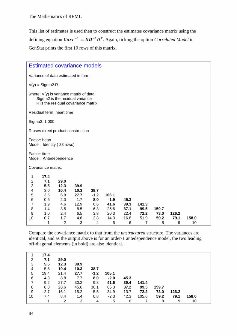
The Mathematics of REML
84
This list of estimates is used then to construct the estimates covariance matrix using the
defining equation . Again, ticking the option Correlated Model in
GenStat prints the first 10 rows of this matrix.
Estimated covariance models
Variance of data estimated in form: V(y) = Sigma2.R where: V(y) is variance matrix of data Sigma2 is the residual variance R is the residual covariance matrix Residual term: heart.time Sigma2: 1.000 R uses direct product construction Factor: heart Model: Identity ( 23 rows) Factor: time Model: Antedependence Covariance matrix: 1 17.4 2 7.1 29.0 3 5.5 12.3 39.9 4 3.0 10.4 10.3 38.7 5 3.5 6.8 27.7 -1.2 105.1 6 0.6 2.0 1.7 8.0 -1.9 45.3 7 1.9 4.6 12.9 6.6 41.6 39.3 141.3 8 1.4 3.5 8.5 6.3 25.6 37.1 99.5 159.7 9 1.0 2.4 6.5 3.8 20.3 22.4 72.2 73.0 126.2 10 0.7 1.7 4.6 2.8 14.3 16.8 51.9 59.2 79.1 158.0
1 2 3 4 5 6 7 8 9 10
Compare the covariance matrix to that from the unstructured structure. The variances are
identical, and as the output above is for an order-1 antedependence model, the two leading
off-diagonal elements (in bold) are also identical.
1 17.4 2 7.1 29.0 3 5.5 12.3 39.9 4 5.8 10.4 10.3 38.7 5 19.4 21.4 27.7 -1.2 105.1 6 4.3 8.8 7.7 8.0 -2.0 45.3 7 9.2 27.7 30.2 9.8 41.6 39.4 141.4 8 6.0 28.6 45.6 30.1 66.3 37.2 99.5 159.7 9 -2.7 16.1 15.2 -5.5 34.9 13.7 72.2 73.0 126.2 10 7.4 8.4 1.4 0.8 -2.3 42.3 105.6 59.2 79.1 158.0
1 2 3 4 5 6 7 8 9 10
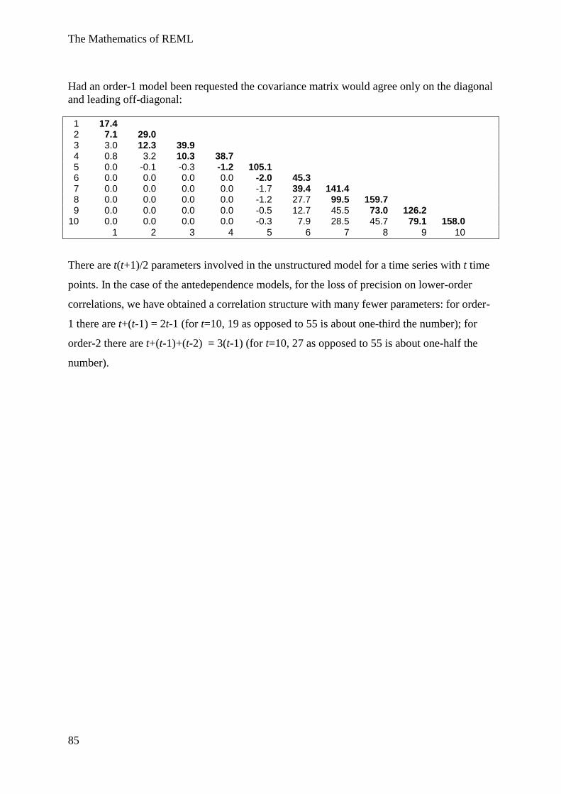
The Mathematics of REML
85
Had an order-1 model been requested the covariance matrix would agree only on the diagonal
and leading off-diagonal:
1 17.4 2 7.1 29.0 3 3.0 12.3 39.9 4 0.8 3.2 10.3 38.7 5 0.0 -0.1 -0.3 -1.2 105.1 6 0.0 0.0 0.0 0.0 -2.0 45.3 7 0.0 0.0 0.0 0.0 -1.7 39.4 141.4 8 0.0 0.0 0.0 0.0 -1.2 27.7 99.5 159.7 9 0.0 0.0 0.0 0.0 -0.5 12.7 45.5 73.0 126.2 10 0.0 0.0 0.0 0.0 -0.3 7.9 28.5 45.7 79.1 158.0
1 2 3 4 5 6 7 8 9 10
There are t(t+1)/2 parameters involved in the unstructured model for a time series with t time
points. In the case of the antedependence models, for the loss of precision on lower-order
correlations, we have obtained a correlation structure with many fewer parameters: for order-
1 there are t+(t-1) = 2t-1 (for t=10, 19 as opposed to 55 is about one-third the number); for
order-2 there are t+(t-1)+(t-2) = 3(t-1) (for t=10, 27 as opposed to 55 is about one-half the
number).
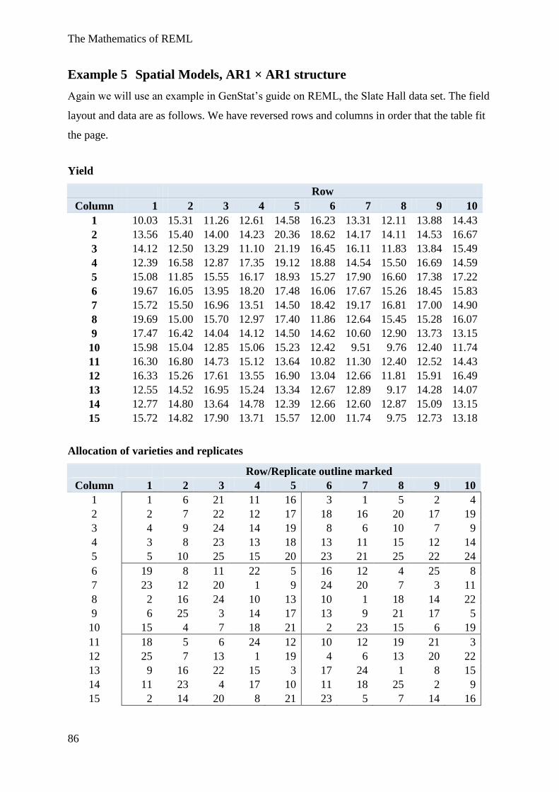
The Mathematics of REML
86
Example 5 Spatial Models, AR1 × AR1 structure
Again we will use an example in GenStat’s guide on REML, the Slate Hall data set. The field
layout and data are as follows. We have reversed rows and columns in order that the table fit
the page.
Yield
Row
Column 1 2 3 4 5 6 7 8 9 10
1 10.03 15.31 11.26 12.61 14.58 16.23 13.31 12.11 13.88 14.43
2 13.56 15.40 14.00 14.23 20.36 18.62 14.17 14.11 14.53 16.67
3 14.12 12.50 13.29 11.10 21.19 16.45 16.11 11.83 13.84 15.49
4 12.39 16.58 12.87 17.35 19.12 18.88 14.54 15.50 16.69 14.59
5 15.08 11.85 15.55 16.17 18.93 15.27 17.90 16.60 17.38 17.22
6 19.67 16.05 13.95 18.20 17.48 16.06 17.67 15.26 18.45 15.83
7 15.72 15.50 16.96 13.51 14.50 18.42 19.17 16.81 17.00 14.90
8 19.69 15.00 15.70 12.97 17.40 11.86 12.64 15.45 15.28 16.07
9 17.47 16.42 14.04 14.12 14.50 14.62 10.60 12.90 13.73 13.15
10 15.98 15.04 12.85 15.06 15.23 12.42 9.51 9.76 12.40 11.74
11 16.30 16.80 14.73 15.12 13.64 10.82 11.30 12.40 12.52 14.43
12 16.33 15.26 17.61 13.55 16.90 13.04 12.66 11.81 15.91 16.49
13 12.55 14.52 16.95 15.24 13.34 12.67 12.89 9.17 14.28 14.07
14 12.77 14.80 13.64 14.78 12.39 12.66 12.60 12.87 15.09 13.15
15 15.72 14.82 17.90 13.71 15.57 12.00 11.74 9.75 12.73 13.18
Allocation of varieties and replicates
Row/Replicate outline marked
Column 1 2 3 4 5 6 7 8 9 10
1 1 6 21 11 16 3 1 5 2 4
2 2 7 22 12 17 18 16 20 17 19
3 4 9 24 14 19 8 6 10 7 9
4 3 8 23 13 18 13 11 15 12 14
5 5 10 25 15 20 23 21 25 22 24
6 19 8 11 22 5 16 12 4 25 8
7 23 12 20 1 9 24 20 7 3 11
8 2 16 24 10 13 10 1 18 14 22
9 6 25 3 14 17 13 9 21 17 5
10 15 4 7 18 21 2 23 15 6 19
11 18 5 6 24 12 10 12 19 21 3
12 25 7 13 1 19 4 6 13 20 22
13 9 16 22 15 3 17 24 1 8 15
14 11 23 4 17 10 11 18 25 2 9
15 2 14 20 8 21 23 5 7 14 16
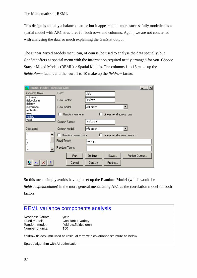
The Mathematics of REML
87
This design is actually a balanced lattice but it appears to be more successfully modelled as a
spatial model with AR1 structures for both rows and columns. Again, we are not concerned
with analysing the data so much explaining the GenStat output.
The Linear Mixed Models menu can, of course, be used to analyse the data spatially, but
GenStat offers as special menu with the information required neatly arranged for you. Choose
Stats > Mixed Models (REML) > Spatial Models. The columns 1 to 15 make up the
fieldcolumn factor, and the rows 1 to 10 make up the fieldrow factor.
So this menu simply avoids having to set up the Random Model (which would be
fieldrow.fieldcolumn) in the more general menu, using AR1 as the correlation model for both
factors.
REML variance components analysis
Response variate: yield Fixed model: Constant + variety Random model: fieldrow.fieldcolumn Number of units: 150 fieldrow.fieldcolumn used as residual term with covariance structure as below Sparse algorithm with AI optimisation
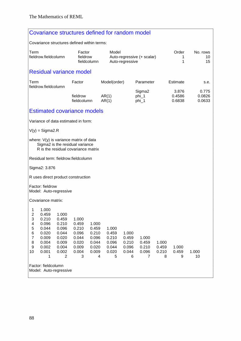
The Mathematics of REML
88
Covariance structures defined for random model Covariance structures defined within terms: Term Factor Model Order No. rows fieldrow.fieldcolumn fieldrow Auto-regressive (+ scalar) 1 10 fieldcolumn Auto-regressive 1 15
Residual variance model Term Factor Model(order) Parameter Estimate s.e. fieldrow.fieldcolumn Sigma2 3.876 0.775 fieldrow AR(1) phi_1 0.4586 0.0826 fieldcolumn AR(1) phi_1 0.6838 0.0633
Estimated covariance models
Variance of data estimated in form: V(y) = Sigma2.R where: V(y) is variance matrix of data Sigma2 is the residual variance R is the residual covariance matrix Residual term: fieldrow.fieldcolumn Sigma2: 3.876 R uses direct product construction Factor: fieldrow Model: Auto-regressive Covariance matrix: 1 1.000 2 0.459 1.000 3 0.210 0.459 1.000 4 0.096 0.210 0.459 1.000 5 0.044 0.096 0.210 0.459 1.000 6 0.020 0.044 0.096 0.210 0.459 1.000 7 0.009 0.020 0.044 0.096 0.210 0.459 1.000 8 0.004 0.009 0.020 0.044 0.096 0.210 0.459 1.000 9 0.002 0.004 0.009 0.020 0.044 0.096 0.210 0.459 1.000 10 0.001 0.002 0.004 0.009 0.020 0.044 0.096 0.210 0.459 1.000 1 2 3 4 5 6 7 8 9 10 Factor: fieldcolumn Model: Auto-regressive
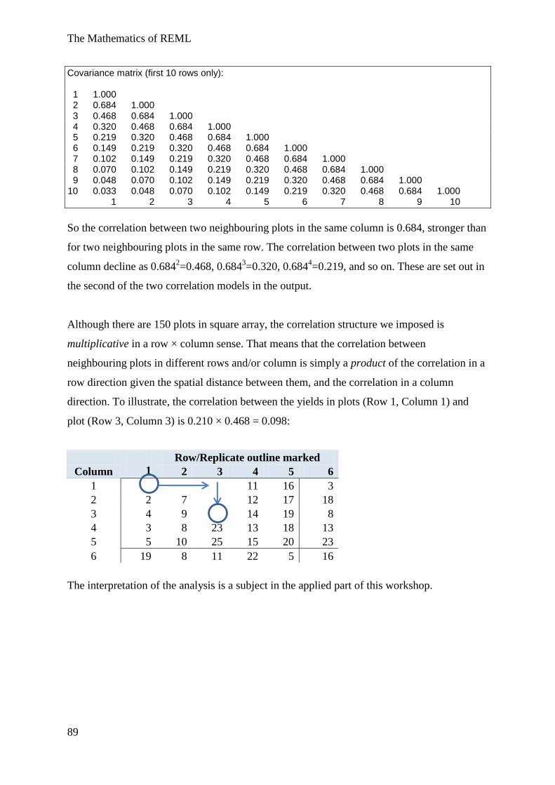
The Mathematics of REML
89
Covariance matrix (first 10 rows only): 1 1.000 2 0.684 1.000 3 0.468 0.684 1.000 4 0.320 0.468 0.684 1.000 5 0.219 0.320 0.468 0.684 1.000 6 0.149 0.219 0.320 0.468 0.684 1.000 7 0.102 0.149 0.219 0.320 0.468 0.684 1.000 8 0.070 0.102 0.149 0.219 0.320 0.468 0.684 1.000 9 0.048 0.070 0.102 0.149 0.219 0.320 0.468 0.684 1.000 10 0.033 0.048 0.070 0.102 0.149 0.219 0.320 0.468 0.684 1.000 1 2 3 4 5 6 7 8 9 10
So the correlation between two neighbouring plots in the same column is 0.684, stronger than
for two neighbouring plots in the same row. The correlation between two plots in the same
column decline as 0.6842=0.468, 0.684
3=0.320, 0.684
4=0.219, and so on. These are set out in
the second of the two correlation models in the output.
Although there are 150 plots in square array, the correlation structure we imposed is
multiplicative in a row × column sense. That means that the correlation between
neighbouring plots in different rows and/or column is simply a product of the correlation in a
row direction given the spatial distance between them, and the correlation in a column
direction. To illustrate, the correlation between the yields in plots (Row 1, Column 1) and
plot (Row 3, Column 3) is 0.210 × 0.468 = 0.098:
Row/Replicate outline marked
Column 1 2 3 4 5 6
1
11 16 3
2 2 7
12 17 18
3 4 9
14 19 8
4 3 8 23 13 18 13
5 5 10 25 15 20 23
6 19 8 11 22 5 16
The interpretation of the analysis is a subject in the applied part of this workshop.