The Mathematics of Logic · applicability not just to philosophical studies in the foundations of...
217
Transcript of The Mathematics of Logic · applicability not just to philosophical studies in the foundations of...

The Mathematics of Logic
A guide to completeness theorems and their applications
This textbook covers the key material for a typical first course in logic for
undergraduates or first year graduate students, in particular, presenting a
full mathematical account of the most important result in logic: the
Completeness Theorem for first-order logic.
Looking at a series of interesting systems increasing in complexity, then
proving and discussing the Completeness Theorem for each, the author
ensures that the number of new concepts to be absorbed at each stage is
manageable, whilst providing lively mathematical applications throughout.
Unfamiliar terminology is kept to a minimum; no background in formal
set-theory is required; and the book contains proofs of all the required set
theoretical results.
The reader is taken on a journey starting with Konig’s Lemma, and
progressing via order relations, Zorn’s Lemma, Boolean algebras, and
propositional logic, to Completeness and Compactness of first-order logic.
As applications of the work on first-order logic, two final chapters provide
introductions to model theory and non-standard analysis.
dr richard kaye is Senior Lecturer in Pure Mathematics at the University
of Birmingham.

The Mathematics of LogicA guide to completeness theoremsand their applications
Richard Kaye
School of Mathematics, University of Birmingham

CAMBRIDGE UNIVERSITY PRESS
Cambridge, New York, Melbourne, Madrid, Cape Town, Singapore, São Paulo
Cambridge University PressThe Edinburgh Building, Cambridge CB2 8RU, UK
First published in print format
ISBN-13 978-0-521-70877-7
ISBN-13 978-0-511-34273-8
© Richard Kaye 2007
2007
Information on this title: www.cambridge.org/9780521708777
This publication is in copyright. Subject to statutory exception and to the provision of relevant collective licensing agreements, no reproduction of any part may take place without the written permission of Cambridge University Press.
ISBN-10 0-511-34273-X
ISBN-10 0-521-70877-X
Cambridge University Press has no responsibility for the persistence or accuracy of urls for external or third-party internet websites referred to in this publication, and does not guarantee that any content on such websites is, or will remain, accurate or appropriate.
Published in the United States of America by Cambridge University Press, New York
www.cambridge.org
paperback
eBook (NetLibrary)
eBook (NetLibrary)
paperback
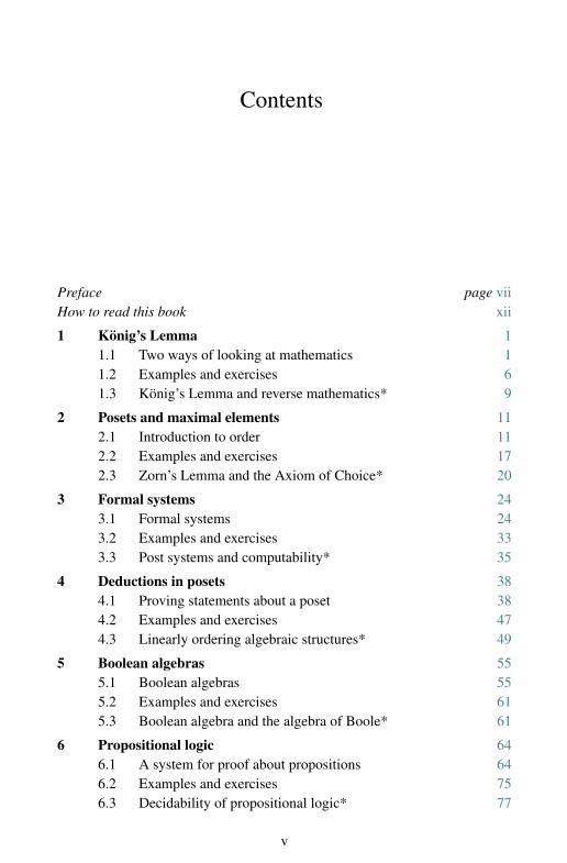
Contents
Preface page viiHow to read this book xii
1 Konig’s Lemma 11.1 Two ways of looking at mathematics 11.2 Examples and exercises 61.3 Konig’s Lemma and reverse mathematics* 9
2 Posets and maximal elements 112.1 Introduction to order 112.2 Examples and exercises 172.3 Zorn’s Lemma and the Axiom of Choice* 20
3 Formal systems 243.1 Formal systems 243.2 Examples and exercises 333.3 Post systems and computability* 35
4 Deductions in posets 384.1 Proving statements about a poset 384.2 Examples and exercises 474.3 Linearly ordering algebraic structures* 49
5 Boolean algebras 555.1 Boolean algebras 555.2 Examples and exercises 615.3 Boolean algebra and the algebra of Boole* 61
6 Propositional logic 646.1 A system for proof about propositions 646.2 Examples and exercises 756.3 Decidability of propositional logic* 77
v

vi Contents
7 Valuations 807.1 Semantics for propositional logic 807.2 Examples and exercises 907.3 The complexity of satisfiability* 95
8 Filters and ideals 1008.1 Algebraic theory of boolean algebras 1008.2 Examples and exercises 1078.3 Tychonov’s Theorem* 1088.4 The Stone Representation Theorem* 110
9 First-order logic 1169.1 First-order languages 1169.2 Examples and exercises 1349.3 Second- and higher-order logic* 137
10 Completeness and compactness 14010.1 Proof of completeness and compactness 14010.2 Examples and exercises 14610.3 The Compactness Theorem and topology* 14910.4 The Omitting Types Theorem* 152
11 Model theory 16011.1 Countable models and beyond 16011.2 Examples and exercises 17311.3 Cardinal arithmetic* 176
12 Nonstandard analysis 18212.1 Infinitesimal numbers 18212.2 Examples and exercises 18612.3 Overspill and applications* 187
References 199Index 200

Preface
Mathematical logic has been in existence as a recognised branch of mathe-matics for over a hundred years. Its methods and theorems have shown theirapplicability not just to philosophical studies in the foundations of mathemat-ics (perhaps their original raison d’etre) but also to ‘mainstream mathematics’itself, such as the infinitesimal analysis of Abraham Robinson, or the morerecent applications of model theory to algebra and algebraic geometry.
Nevertheless, these logical techniques are still regarded as somewhat ‘diffi-cult’ to teach, and possibly rather unrewarding to the serious mathematician. Inpart, this is because of the notation and terminology that still survives as a relicof the original reason for the subject, and also because of the off-putting anddidactically unnecessary logical precision insisted on by some of the authorsof the standard undergraduate textbooks. This is coupled by the professionalmathematician’s very reasonable distrust of so much emphasis on ‘inessen-tial’ non-mathematical details when he or she only requires an insight into themathematics behind it and straightforward statements of the main mathemati-cal results.
This book presents the material usually treated in a first course in logic, butin a way that should appeal to a suspicious mathematician wanting to see somegenuine mathematical applications. It is written at a level suitable for an un-dergraduate, but with additional optional sections at the end of each chapterthat contain further material for more advanced or adventurous readers. Thecore material in this book assumes as prerequisites only: basic knowledge ofpure mathematics such as undergraduate algebra and real analysis; an interestin mathematics; and a willingness to discover and learn new mathematical ma-terial. The main goal is an understanding of the mathematical content of theCompleteness Theorem for first-order logic, including some of its mathemat-ically more interesting applications. The optional sections often require addi-tional background material and more ‘mathematical maturity’ and go beyond a
vii

viii Preface
typical first undergraduate course. They may be of interest to beginning post-graduates and others.
The intended readership of this book is mathematicians of all ages and per-suasions, starting at third year undergraduate level. Indeed, the ‘unstarred’sections of this book form the basis of a course I have given at BirminghamUniversity for third and fourth year students. Such a reader will want a goodgrounding in the subject, and a good idea of its scope and applications, but ingeneral does not require a highly detailed and technical treatment.
On the other hand, for a full mathematical appreciation of what the Com-pleteness Theorem has to offer, a detailed discussion of some naive set theory,especially Zorn’s Lemma and cardinal arithmetic, is essential, and I make noapology for including these in some detail in this book.
This book is unusual, however, since I do not present the main concepts andgoals of first-order logic straight away. Instead, I start by showing what themain mathematical idea of ‘a completeness theorem’ is, with some illustra-tions that have real mathematical content. The emphasis is on the content andpossible applications of such completeness theorems, and tries to draw on thereader’s mathematical knowledge and experience rather than any conception(or misconception) of what ‘logic’ is.
It seems that ‘logic’ means many things to different people, from puzzlesthat can be bought at a newsagent’s shop, to syllogisms, arguments using Venndiagrams, all the way to quite sophisticated set theory. To prepare the readerand summarise the idea of a completeness theorem here, I should say a littleabout how I regard ‘logic’.
The principal feature of logic is that it should be about reasoning or deduc-tion, and should attempt to provide rules for valid inferences. If these rulesare sufficiently precisely defined (and they should be), they become rules formanipulating strings of symbols on a page. The next stage is to attach mean-ing to these strings of symbols and try to present mathematical justification forthe inference rules. Typically, two separate theorems are presented: the firstis a ‘Soundness Theorem’ that says that no incorrect deductions can be madefrom the inference rules (where ‘correct’ means in terms of the meanings weare considering); the second is a ‘Completeness Theorem’ which says that allcorrect deductions that can be expressed in the system can actually be madeusing a combination of the inference rules provided. Both of these are precisemathematical theorems. Soundness is typically the more straightforward of thetwo to prove; the proof of completeness is usually much more sophisticated.Typically, it requires mathematical techniques that enable one to create a newmathematical ‘structure’ which shows that a particular supposed deduction thatis not derivable in the system is not in fact correct.

Preface ix
Thus logic is not only about such connectives as ‘and’ and ‘or’, though themain systems, including propositional and first-order logic, do have symbolsfor these connectives. The power of the logical technique for the mathemati-cian arises from the way the formal system of deduction can help organisea complex set of conditions that might be required in a mathematical con-struction or proof. The Completeness Theorem becomes a very general andpowerful way of building interesting mathematical structures. A typical ex-ample is the application of first-order logic to construct number systems withinfinitesimals that can used rigorously to present real calculus. This is the so-called nonstandard analysis of Abraham Robinson, and is presented in the lastchapter of this book.
The mathematical content of completeness and soundness is well illustratedby Konig’s Lemma on infinite finitely branching trees, and in the first chapter Idiscuss this. This is intended as a warm-up for the more difficult mathematicsto come, and is a key example that I refer back to throughout the book.
Zorn’s Lemma is essential for all the work in this book. I believe that by finalyear level, students should be starting to master straightforward applications ofZorn’s Lemma. This is the main topic in Chapter 2. I do not shy away fromthe details, in particular giving a careful proof of Zorn’s Lemma for countableposets, though the details of how Zorn’s Lemma turns out to be equivalent tothe Axiom of Choice is left for an optional section.
The idea of a formal system and derivations is introduced in Chapter 3, witha system based on strings of 0s and 1s that turns out to be closely related toKonig’s Lemma. In the lecture theatre or classroom, I find this chapter to beparticularly important and useful material, as it provides essential motivationfor the Soundness Theorem. Given a comparatively simple system such as this,and asked whether a particular string σ can be derived from a set of assump-tions Σ, students are all too ready to answer ‘no’ without justification. Wherejustification is offered, it is often of the kind, ‘I tried to find a formal proof andthis was my attempt, but it does not work.’ So the idea of a careful proof by in-duction on the length of a formal derivation (and a carefully selected inductionhypothesis) can be introduced and discussed without the additional compli-cation of a long list of deduction rules to consider. The idea of semantics,and the Soundness and Completeness Theorems, arises from an investigationof general methods to show that certain derivations are not possible, and, toillustrate their power, Konig’s Lemma is re-derived from the Soundness andCompleteness Theorems for this system.
The reader will find systems with mathematically familiar derivations forthe first time in Chapter 4. Building on previous material on posets, I developa system for derivations about a poset, including rules such as ‘if a < b and

x Preface
b < c then a < c’. The system also has a way of expressing statements of theform ‘a is not less than b’, and this is handled using a Reductio Ad AbsurdumRule, a rule that is used throughout the rest of the book. By this stage, itshould be clear what the right questions to ask about the system are, and themathematical significance of the Completeness Theorem (the construction ofa suitable partial order on a set) is clear. As a bonus, two pretty applicationsare provided: that any partial order can be ‘linearised’; and that from a set of‘positive’ assumptions a ‘negative’ conclusion can always be strengthened toa ‘positive’ one.
The material normally found in a more traditional course on mathemati-cal logic starts with Chapter 5. Chapters 5 to 8 discuss boolean algebras andpropositional logic. My proof system for propositional logic is chosen to be aform of natural deduction, but set out in a linear form on the page with clearlydelineated ‘subproofs’ rather than a tree structure. This seems to be closest toa student’s conception of a proof, and also provides clear proof strategies sothat exercises in writing proofs can be given in a helpful and relatively painlessway. (I emphasise the word ‘relatively’. For most students, this aspect of logicis never painless, but at least the system clearly relates to informal proofs theymight have written in other areas of mathematics.) I do not avoid explaining theprecise connections between propositional logic and boolean algebra; these areimportant and elegant ideas, and are accessible to undergraduates who shouldbe able to appreciate the analogies with algebra, especially rings and fields.More advanced students will also appreciate the fact that deep results such asTychonov’s Theorem and Stone Duality are only a few pages extra in an op-tional section. However, if time is short, the chapter on filters and ideals canbe omitted entirely.
Chapters 9 and 10 are the central ones that cover first-order logic and themain Completeness Theorem. Apart from the choice of formal system (adevelopment of the natural deduction system already used for propositionallogic) they follow the usual pattern. These chapters are the longest in the bookand will be found to be the most challenging so I have deliberately avoidedmany of the technically tricky issues such as: unique readability; the formaldefinition of the scope of a quantifier; or when a variable may be substitutedby a term. An intelligent reader at this level using his or her basic mathemat-ical training and intuition and following the examples is sure to do the ‘rightthing’ and does not want to be bogged down in formal syntactic details. Thesetechnical details are of course important later on if one becomes involved informalising logic in a first-order system such as set theory or arithmetic. Butthe place for that sort of work is certainly not a first course in logic. For thosereaders that need it, further details are available on the companion web-pages.

Preface xi
The method of proof of the Completeness Theorem is by ‘Henkinising’ thelanguage and then using Zorn’s Lemma to find a maximal consistent set ofsentences. This is easier to describe to first-timers than tree-constructions ofsets of consistent sentences with their required inductive properties, but is justas general and applicable. Two bonus optional sections for adventurous stu-dents with background in point-set topology include a topological view of theCompactness Theorem, and a proof of the full statement of the Omitting TypesTheorem via Baire’s Theorem, which is proved where needed.
Chapters 11 and 12 (which are independent of each other) provide appli-cations of first-order logic. Chapter 11 presents an introduction to model the-ory, including the Lowenheim–Skolem Theorems, and (to put these in context)a short survey of categoricity, including a description of Morley’s Theorem.This chapter is where infinite cardinals and cardinal arithmetic are used for thefirst time, and I carefully state all the required ideas and results before usingthem. Full proofs of these results are given in an optional section, using Zorn’sLemma only. The traditional options of using ordinals or the well-orderingprinciple are avoided as being likely to beg more questions than they an-swer to students without any prior knowledge in formal set theory. Chap-ter 12 presents an introduction to nonstandard analysis, including a proof of thePeano Existence Theorem on first-order differential equations. My presenta-tion of nonstandard analysis is chosen to illustrate the main results of first-orderlogic and the interplay between the standard and nonstandard worlds, ratherthan to be optimal for fast proofs of classical results by nonstandard methods.
I have enjoyed writing this book and teaching from it. The material hereis, to my mind, much more exciting and varied than the standard texts I learntfrom as an undergraduate, and responses from the students who were givenpreliminary versions of these notes were good too. I can only hope that you,the reader, will derive a similar amount of pleasure from this book.

How to read this book
Chapters are deliberately kept as short as possible and discuss a single math-ematical point. The chapters are divided into sections. The first section ofeach chapter is essential reading for all. The second section generally containsfurther applications, examples and exercises to test and expand on material pre-sented in the previous section, and is again essential to read and explore. Oneor more extra ‘starred’ sections are then added to provide further commentaryon the key material of the chapter and develop the material. These other sec-tions are not essential reading and are intended for more inquisitive, ambitiousor advanced readers with the background knowledge required. Chapter 8 maybe omitted if time is short, and Chapters 11 and 12 are independent of eachother.
Mathematical terminology is standard or explained in the text. Bold faceentries in the index refer to definitions in the text; other entries provide furtherinformation on the term in question.
Additional material, including some technical definitions that I have chosento omit in the printed text for the sake of clarity, further exercises, discussion,and some hints or answers to the exercises here, will be found on the compan-ion web-site at http://web.mat.bham.ac.uk/R.W.Kaye/logic.
xii
1
Konig’s Lemma
1.1 Two ways of looking at mathematics
It seems that in mathematics there are sometimes two or more ways of provingthe same result. This is often mysterious, and seems to go against the grain,for we often have a deep-down feeling that if we choose the ‘right’ ideas ordefinitions, there must be only one ‘correct’ proof. This feeling that thereshould be just one way of looking at something is rather similar to Paul Erdos’sidea of ‘The Book’ [1], a vast tome held by God, the SF, in which all the best,most revealing and perfect proofs are written.
Sometimes this mystery can be resolved by analysing the apparently differ-ent proofs into their fundamental ideas. It often turns out that, ‘underneath thebonnet’, there is actually just one key mathematical concept, and two seem-ingly different arguments are in some sense ‘the same’. But sometimes therereally are two different approaches to a problem. This should not be disturbing,but should instead be seen as a great opportunity. After all, two approaches tothe same idea indicates that there are some new mathematics to be investigatedand some new connections to be found and exploited, which hopefully willuncover a wealth of new results.
I shall give a rather simple example of just the sort of situation I have inmind that will be familiar to many readers – one which will be typical of thekind of theorem we will be considering throughout this book.
Consider a binary tree. A tree is a diagram (often called a graph) witha special point or node called the root, and lines or edges leaving this nodedownwards to other nodes. These again may have edges leading to furthernodes. The thing that makes this a tree (rather than a more general kind ofgraph) is that the edges all go downwards from the root, and that means thetree cannot have any loops or cycles. The tree is a binary tree if every node isconnected to at most two lower nodes. If every node is connected to exactly
1

2 Konig’s Lemma
�/0
�0 �1
�00 �01 �10 �11
�000 �001 �010 �011 �100 �101 �110 �111
� � � � � � � � � � � � � � � �
Figure 1.1 The full binary tree.
�/0
�0 �1
�00 �01 �10 �11
�000 �001 �100 �101 �110 �111
� � � � � � �
Figure 1.2 A binary tree.
two lower nodes, the tree is called the full binary tree. Note that in general,a node in a binary tree may be connected to 0, 1 or 2 lower nodes. We willlabel the nodes in our trees with sequences of integers. It is convenient to makelabels for the nodes below the node that has label x by adding either the digit 0or 1 to the end of x, giving x0 and x1. Figure 1.1 illustrates the full binary tree,whereas Figure 1.2 gives a typical (non-full) binary tree.

1.1 Two ways of looking at mathematics 3
Trees are very important in mathematics, because many constructions followtrees in some way or other. Binary trees are especially interesting since awalk along a tree, following a path that starts at the root, has at most twochoices of direction at every node. Binary trees arise quite naturally in manymathematical ideas and proofs and general theorems about them can be quitepowerful and useful. One of the better known and more useful of these resultsis called Konig’s Lemma.
To explain Konig’s Lemma, consider what it means for a tree T to be infinite.There are two viewpoints, and two possible definitions.
Firstly, suppose you have somehow drawn the whole of the tree T on paperor on the blackboard and are inspecting it. You are in a fortunate position to beable to take in every one of its features, and to examine every one of its nodesand edges. You will quite naturally say that the tree is infinite if it has infinitelymany nodes, or – amounting to the same thing – infinitely many edges. This isa sort of ‘definition from perfect information’ and is similar to what logicianscall semantics, though we will not see the connection with semantics and thetheory of ‘meaning’ for a while.
Now consider you are an ant walking on the binary tree T , which is againdrawn in its entirety on paper. You start at the root node, and you follow theedges, like ant tracks, which you hope will take you to something interesting.Unlike the mathematician viewing the tree in its entirety, you can only see thenode you are at and the edges leaving it. If you take a walk down the tree,you may have choices of turning left or right at any given node and continuingyour path. But it is possible that you have no choice at all, because eitherthere is only one edge out of the node other than the one you entered it by,or possibly there is no such edge at all, in which case your walk has cometo an end. To the ant, which cannot perceive the whole of the tree, but justfollows paths, there is a quite different idea of what it means for the tree to beinfinite: the ant would say that T is infinite if it can find somehow (by guessingthe right combination of ‘left’ and ‘right’ choices) an infinite path through thetree. The ant’s definition of ‘infinite’ might be thought of as a ‘definition fromimperfect information’ and is similar to the logician’s idea of proof. If youlike, you can think of an infinite path chosen by the ant as a proof that the treeis infinite. Like all proofs, it supports the claim made, without giving muchextra information – such as what the tree looks like off this path.
Konig’s Lemma is the statement that, for binary trees, these two ideas ofa tree being infinite are the same. It is in fact a rather useful statement withmany interesting applications. The key feature of this statement is that it re-lates two definitions, one mathematical definition working from perfect or total
4 Konig’s Lemma
information, and one working from the point of view of much more limited in-formation, and shows that they actually say the same thing.
As with all ‘if and only if’ theorems, there are two directions that must beproved. The first, that if there is an infinite path through the tree then the treeis infinite, is immediate. This easier direction is called a Soundness Theoremsince it says the ant’s perception based on partial information is sound, or inother words will not result in erroneous conclusions. The other direction isthe non-trivial one, and its mathematical strength lies in the way it states thata rather general mathematical situation (that the tree is infinite) can always bedetected in a special way from partial information. The reason why it is calledCompleteness will be discussed later in relation to some other examples.
This has been a long preliminary discussion, but I hope it has proved illumi-nating. We shall now turn to the more formal mathematical details and definetree, path, etc., and then state and prove Konig’s Lemma properly.
Definition 1.1 The set of natural numbers, N, will be taken in this book to be{0, 1, 2, . . .}.
For those readers who expect the natural numbers to start with 1, I can onlysay that I appreciate that there are occasions when it is convenient to forgetabout zero, but for me zero is very natural, probably the most logically naturalnumber of all, so is included here in the set of natural numbers.
Definition 1.2 A sequence is a function s whose domain is either the set N
of all natural numbers or a subset of it of the form {x ∈ N : x < n} for somen ∈N. Normally the values of the sequence will be numbers, 0 or 1 say, but thedefinition above (with n = 0) allows the empty sequence with no values at all.We write a sequence by listing its values in order, for example as 00110101001or 0101010101. The length of a sequence is the number of elements in thedomain of the function. This will always be a natural number or infinity.
Definition 1.3 If s is a sequence of length l and n ∈ N is at most l, then s � ndenotes the initial part of s of length n.
For example, if s = 00100011 then s � 4 = 0010.
Definition 1.4 If s is a sequence of length l and x is 0 or 1 then sx is thesequence of length l + 1 whose last element is x and all other elements agreewith those of s.
Our definition of a tree is of a set of sequences that is closed under therestriction operation � .

1.1 Two ways of looking at mathematics 5
Definition 1.5 A tree is a set of sequences T such that for any s ∈ T of lengthn and for any l < n then s � l ∈ T .
Think of a sequence s ∈ T as a finite path starting from the root and arrivingat some node. The individual digits in the sequence determine which choice ofedge is made at each node. The set of nodes of the whole tree is then the set ofsequences in the set T and two nodes s, t ∈ T are connected by a single edgeif one can be got from the other by adding a single number to the sequence. Inother words, s and t are connected if s � (n−1) = t when s is the longer of thetwo and has length n, or the other way round if t is longer. Then the conditionin the definition says, not unreasonably, that each node that this path passesthrough must also be in the tree. The root of the tree is the empty sequence oflength 0.
Definition 1.6 A subtree of a tree T is a subset S of T that is a tree in its ownright.
A subtree of a tree T might contain fewer nodes, and therefore fewer choicesat certain nodes.
Definition 1.7 A binary tree is a tree T where all the sequences in it arefunctions from some {n ∈ N : n < k} to {0, 1}.
In other words, at any node, a path from the root of a binary tree has at mosttwo options: to go left (0) or right (1). However, it may turn out that only one,or possibly neither, of these options is available at a particular node.
Definition 1.8 A tree T is infinite if it contains infinitely many sequences, or(equivalently) has infinitely many nodes.
A path is a subtree with no branching allowed. That means for any twonodes in the tree, one is a ‘predecessor’ of the other. More formally, we havethe following definition.
Definition 1.9 A path, p, in a tree T is a subtree of T such that for any s, t ∈ pwith lengths n, k respectively and n � k, we have s = t � n.
A tree T containing an infinite path p is obviously infinite. Konig’s Lemmastates that the converse is also true for binary trees.
Theorem 1.10 (Konig’s Lemma) Let T be an infinite binary tree. Then Tcontains an infinite path p.

6 Konig’s Lemma
Proof Suppose T is an infinite binary tree. For a sequence s of length n letTs be {r ∈ T : r � n = s}∪ {s � k : k < n}, which we will call the subtree of Tbelow s. You will be able to check easily that Ts is a tree. In general it may ormay not be infinite.
We are going to find a sequence s(n) of elements of T such that
• s(n) has length n,• s(n) = s(n+1) � n,• the tree Ts(n) below s(n) is infinite.
This construction is by induction, using the third property above as our in-duction hypothesis. When we have completed the proof the set {s(n) : n ∈ N}will be our infinite path p in T .
So suppose inductively that we have chosen s = s(n) of length n and Ts isinfinite. Then since the tree is binary, made from sequences of 0s and 1s, wehave
Ts = {r ∈ T : r � (n+1) = s0}∪{r ∈ T : r � (n+1) = s1}∪{s � k : k � n} .
This is, by the induction hypothesis, infinite. Hence (as the third of these threesets is obviously finite) at least one of the first two sets, corresponding to ‘0’ or‘1’ respectively, is infinite. If the first of these is infinite we set s(n + 1) = s0and in this case we have
Ts(n+1) = {r ∈ T : r � (n+1) = s0}∪{s0}∪{s � k : k � n}which is infinite. If not we set s(n+1) = s1 which would then be infinite as be-fore. Either way we have defined s(n+1) and proved the induction hypothesisfor n+1.
1.2 Examples and exercises
The central theorem of this book, the Completeness Theorem for first-orderlogic, is not only of the same flavour as Konig’s Lemma, but is in fact a pow-erful generalisation of it. To give you an idea of the power that this sort oftheorem has, it is useful to see a selection of applications of Konig’s Lemmahere.
We start by exploring the limits of Konig’s Lemma a little: it turns out thatthe important thing is not that there are at most two choices at each node butthat the number of ways in which the branches divide is always finite.
Definition 1.11 If T is a tree and s ∈ T is a node of T then the valency ordegree of s is the number of nodes of T connected to s. Thus this is the number

1.2 Examples and exercises 7
of x such that sx ∈ T plus one (to cater for the edge back towards the root), orjust the number of such x if s is the root node.
Exercise 1.12 Prove the following generalisation of Konig’s Lemma: an infi-nite tree in which every vertex has finite valency has an infinite path. Assumethat the tree has vertices or nodes which are sequences of natural numbers offinite length and that for each s ∈ T there is a bound Bs ∈ N on the possiblevalues x such that sx ∈ T .
There are two ways that you might have done the last exercise. You mighthave modified the proof given above, or you may have tried to reduce thecase of arbitrary finite valency trees to the case of binary trees by somehow‘encoding’ arbitrary finite branching by a series of binary branches.
Exercise 1.13 Whichever method you used, have a go at proving the extensionof Konig’s Lemma by the other method.
Exercise 1.14 By giving an appropriate example of an infinite tree, show thatKonig’s Lemma is false for graphs with vertices of infinite valency.
Konig’s Lemma is an elegant but nevertheless not very surprising or difficultresult to see. Its truth, it seems, is reasonably clear, though a completely rigor-ous proof takes a moment or two to come up with. It is all the more surprising,therefore that there should be non-trivial applications. We will look at a few ofthese now, though nothing later in this book will depend on them.
Example 1.15 The set X = [0, 1] has the property (called sequential compact-ness, equivalent to compactness for metric spaces) that every sequence (an) ofelements of X has a subsequence converging to some element in X .
Proof Starting with [0, 1] we continually divide intervals into equal halves,but at stage k of the construction we throw away any such interval that con-tains none of the an with n > k. More precisely, the nodes of the tree atdepth k are identified with intervals I = [(r − 1)2−k, r2−k] for which r ∈ N
and {an : n > k and an ∈ I} is non-empty, and two nodes are connected if oneis a subset of the other.
This defines a binary tree. It is infinite because there are infinitely manyan and each lies in an interval. By Konig’s Lemma there is an infinite paththrough this tree, and by the construction of the tree we may take an infinitesubsequence of an in this path, one at each level of the tree. This is the requiredconvergent subsequence.
8 Konig’s Lemma
Now consider infinite sequences u0u1u2. . . of the digits 0, 1, 2, . . ., k− 1. Wewill call such sequences k-sequences. Say a k-sequence s is xn-free if there isno finite sequence, x, of digits 0, 1, 2, . . ., k− 1, such that the finite sequencexn (defined to be the result of repeating and concatenating x as xxxx. . .x, wherethere are n copies of the string x) does not appear as a contiguous block of thesequence s.
Exercise 1.16 (a) Show that there is no x2-free 2-sequence.(b) Use Konig’s Lemma to show that there is an x3-free 2-sequence if and
only if there are arbitrarily long finite x3-free 2-sequences. State and prove asimilar result for x2-free 3-sequences.
(c) Define an operation on finite 2-sequences σ such that σ(0) = 01, σ(1) =10, and σ(u0u1. . .um) = σ(u0)σ(u1). . .σ(um), where this is concatenation ofsequences. Let σn(s) = σ(σ(. . .(σ(s)). . .)), i.e. σ iterated n times. Show thateach of the finite sequences σn(0) is x3-free, and hence there is an infinitex3-free 2-sequence.
(d) Show there is an x2-free 3-sequence.
Another example of the use of Konig’s Lemma is for graphs in the plane. Agraph is a set V of vertices and a set E of edges, which are unordered subsets ofV with exactly two vertices in each edge. In a planar graph the set of verticesV is a set of points of R2, and the edges joining vertices are lines which are‘smooth’ (formed from finitely many straight-line segments) and may not crossexcept at a vertex.
A graph with set of vertices V can be k-coloured if there is a map f : V →{0, 1, . . ., k−1} such that f (u) �= f (v) for all vertices u, v that are joined byan edge. You should think of the values 0, 1, . . ., k − 1 as ‘colours’ of thevertices; the condition says two adjacent vertices must be coloured differently.Graph colourings, and especially colourings of planar graphs, are particularlyinteresting and have a long history [12]. A deep and difficult result by Appeland Haken shows that every finite planar graph is 4-colourable [10].
Exercise 1.17 Use Konig’s Lemma to show that an infinite graph can be k-coloured if and only if every finite subgraph of it can be so coloured. (Make thesimplification that the vertices of our infinite graph can be ordered as v0, v1, . . .
with indices from N. Construct a tree where the nodes at level n are all k-colourings of the subgraph with vertices v0, v1, . . ., vn−1, and edges join nodesif one colouring extends another.) Deduce from Appel and Haken’s result thatevery infinite planar graph can be 4-coloured.
Tiling problems provide another nice application of Konig’s Lemma. Con-
1.3 Konig’s Lemma and reverse mathematics* 9
sider a finite set of tiles which are square, with special links like jigsaw piecesso that in a tiling with tiles fitting together, one edge of one tile must be nextto one of certain edges of other tiles. A tiling of the plane is a tiling usingany number of tiles of each of the finitely many types, so that the whole of theplane is covered. Tiling problems ask whether the plane can or cannot be tiledusing a particular set.
Exercise 1.18 Prove that a finite set of tiles can tile the plane if and only ifevery finite portion of the plane can be so tiled.
Finally, for this section, trees are also useful for describing computations.We will not define any idealised computer here, nor provide any backgroundin computability theory, so this next example is for readers with such back-ground, or who are willing to suspend judgement until they have such back-ground. Normally, computations are deterministic, that is every step is deter-mined completely by the state of the machine. A non-deterministic computa-tion is one where the computer has a fixed number, B, of possible ‘next moves’at any stage. The machine is allowed to choose one of these ‘at random’, orby making a ‘lucky guess’ and in so doing it hopes to verify that some asser-tion is true. This gives rise to a computation tree of all possible computations.Suppose we somehow know in advance that whatever choices are made at anystep, every computation of the machine will eventually halt and give an answer.That means that all paths through the computation tree are finite. Then by thecontrapositive of Konig’s Lemma the tree is finite. This means that the non-deterministic computation can be simulated in finite time by a deterministicone which constructs the computation tree in memory and analyses it.
1.3 Konig’s Lemma and reverse mathematics*
Konig’s Lemma is rather attractive and has some pretty applications. It hasbeen ‘traditional’ in logic textbooks to give some of the examples above asapplications of the much more powerful ‘Completeness Theorem for first-orderlogic’. Whilst not incorrect, this has always seemed a pity to me, as it hardlydoes the Completeness Theorem justice when the applications can be proveddirectly from the more familiar Konig’s Lemma. Suffice it to say for nowthat there will be plenty of interesting applications of the full CompletenessTheorem that cannot be argued from Konig’s Lemma alone.
It may be a good idea to say a few words about why Konig’s Lemma is pow-erful, and where it does real mathematical work. The reason is that, althoughthere may be an infinite path in a tree, it is not always clear how to find one,

10 Konig’s Lemma
and in any case there are likely to be choices involved. In our proof of Konig’sLemma, to keep track of all these individual choices, we used the concept of acertain subtree Ts being infinite. Being ‘infinite’ is of course a powerful math-ematical property, and one about which there is a lot that can be said, bothwithin and outside the field of mathematical logic. This concept of an infinitesubtree is doing quite a lot of work for us here, especially as it is being usedinfinitely many times in the course of an induction.
Some workers in the logic community study these ideas in more detail bytrying to identify which theorems need which lemmas to prove them. Thisarea of logic is often called reverse mathematics since the main aim is usuallyto prove the axioms from the theorems. I am not going to advocate reversemathematics here, but there are plenty of times when it is nice to know that acomplicated lemma cannot be avoided in a proof. It is certainly true for manyof the exercises in the previous section that Konig’s Lemma (or something verymuch like it) is necessary for their solution. In reverse mathematics one usuallyworks from a weaker set of axioms, one where the concept of an infinite setis not available. It turns out, for example, that relative to this weak set ofaxioms the sequential compactness of [0, 1] is actually equivalent to Konig’sLemma. For more information on reverse mathematics see the publications byHarvey Friedman, Stephen Simpson and others, in particular Simpson’s 2001volume [11].
The proof of Konig’s Lemma works, as we have seen, by making a seriesof choices. The issue of making choices is also a very subtle one, but onethat will come up in many places in this book. We can always make finitelymany choices as part of a proof, by just listing them. (In this way, to maken choices in a proof you will typically need at least n lines of proof, for eachn ∈ N.) But making infinitely many choices in one proof, or even an unknownfinite number of choices, will depend on being able to give a rule stating whichchoice is to be made and when. This might be more difficult to achieve. Someversions of Konig’s Lemma do indeed involve infinitely many arbitrary choicesas we turn ‘left’ or ‘right’ following an infinite path. This is a theme that willbe taken up in the next chapter. As a taster, you could attempt the followingexercise, a more difficult version of Exercise 1.12.
Exercise 1.19 Consider the generalisation of Konig’s Lemma that says that aninfinite tree T in which every vertex has finite valency has an infinite path. Donot make any simplifying assumptions on the elements of the sequences s ∈ T .What choices have to be made in the course of the proof, and how might youspecify all of these choices unambiguously in your proof?

2
Posets and maximal elements
2.1 Introduction to order
The idea of an order is central to many kinds of mathematics. The real num-bers are familiarly ordered as a number-line, and even a collection of sets willbe seen to be partially ordered by the ‘subset of’ relation. We shall start by pre-senting the axioms for a partially ordered set and then discuss one particularlyinteresting question about such sets, whether they have maximal elements.
An order relation is a relation R between elements x, y of some set X , wherexRy means x is smaller than or comes before y. An alternative notation ariseswhen one thinks of the relation more concretely as a set of pairs (x, y), a subsetof X2 = {(x, y) : x, y ∈ X}. We can then write xRy in an alternative way as(x, y) ∈ R.
Definition 2.1 A partial order on a set X is a relation R ⊆ X2 such that
(i) (x, y) ∈ R and (y, z) ∈ R implies (x, z) ∈ R(ii) (x, x) �∈ R
for all x, y ∈ X .
Example 2.2 The relation on the set of real numbers R defined by ‘(x, y) ∈ Rif and only if x < y’ is a partial order, where < is the usual order on the set ofreal numbers. In fact it is a special kind of partial order that we will later calla total order or linear order.
Example 2.3 If X is any set and P is its power set, i.e. the set of all subsetsof X , then the relation R on P given by (A, B) ∈ R if and only if A is a propersubset of B (i.e. A ⊆ B and A �= B) is also a partial order on P.
We usually use a symbol such as <, etc., for our relation R and when we dowe write x < y instead of (x, y) ∈ R.
11

12 Posets and maximal elements
There is another kind of partial order relation corresponding to � instead of<. Here, the order relation is allowed to relate equal elements. In other words,we will allow (x, x) ∈ R to be true. (This was explicitly disallowed for the firstkind of order as defined above.) Clearly we will need different axioms for suchan order relation, and the axioms we choose are as follows.
Definition 2.4 A non-strict partial order on a set X is a binary relation R ⊆ X2
such that
(i) (x, y) ∈ R and (y, z) ∈ R implies (x, z) ∈ R(ii) (x, x) ∈ R
(iii) (x, y) ∈ R and (y, x) ∈ R implies x = y
for all x, y ∈ X .
We usually use a symbol such as �, etc., for a non-strict partial order. Thefirst kind of partial order is sometimes called a strict partial order to distinguishit from the non-strict case.
If X is any set and P is its power set, then the relation S on P given by(A, B) ∈ S if and only if A is a subset of B is a non-strict partial order on Pbecause of the law that says two sets A and B are the same if and only if A ⊆ Band B ⊆ A.
If < is a strict partial order on X then we can turn it into a non-strict partialorder � by defining x � y if and only if x < y or x = y. In the other direction,given a non-strict partial order � on X then we can define a strict partial orderby x < y if and only if x � y and x �= y. If we start with one kind of order and doboth of these processes, we get back to the original order relation, so strict andnon-strict partial orders are versions of the same idea. Some of the exercisesdiscuss these points further.
Definition 2.5 A poset is a non-empty set X with a partial order of either thestrict or non-strict variety.
The word poset is an abbreviation for Partially Ordered SET. Unless a dif-ferent notation for the order relation is given, we shall use < for the strictpartial order on X and � for its non-strict version.
Example 2.6 Let T be a binary tree, i.e. a set of finite sequences of 0s and 1swhich is closed under taking initial segments. Define σ � τ to mean that σ isan initial segment of τ . Then this is a (non-strict) partial order on T and makesT into a poset.

2.1 Introduction to order 13
There will be several occasions throughout this book where we will be in-terested in the notion of a maximal element in a poset. This is defined next.
Definition 2.7 If X is a poset and x ∈ X , we say that x is a maximal element ofX if there is no y in x such that x < y.
Be careful how you read this. The element x is maximal if there is nothingbigger. This is not the same as saying that x is the biggest element. Indeeda poset may have several maximal elements, as we will see, but there canobviously only be one biggest element.
Example 2.8 In the poset P of the set of all subsets of X , with (non-strict)order relation ⊆, there is a maximal element, X itself. This is because if A ∈ Pthen A ⊆ X so we cannot have X ⊆ A and X �= A. In fact X is the only maximalelement since A ⊆ X for all A ∈ P, so no A �= X can also be maximal.
Example 2.9 In the poset R of the reals with the usual ordering there are nomaximal elements.
Example 2.10 Let X = {1, 2, 3}, and let Q be the set of all subsets of X withat most two elements. This is a poset with the same ⊆ ordering. In this casethere are three distinct maximal elements, {2, 3}, {1, 3}, and {1, 2}.
As we have seen in the examples, some posets have a unique maximal el-ement, some have many, and some have none. We are going to discuss somecriteria that can be used to determine whether a particular poset has a maximalelement. First, we say a poset is finite if its underlying set X is finite. Then wehave the following theorem.
Theorem 2.11 Any finite poset has at least one maximal element.
Proof This is another proof that involves making choices, somewhat similarto those in the last chapter. Fortunately, only finitely many are required in thiscase. Let X be our finite poset and let a ∈ X . Let a0 = a. We are going todefine a sequence of elements an ∈ X such that an < an+1 for each n.
Given an ∈ X , there are two possibilities. Either an is maximal, in whichcase we are finished, or else there is some b ∈ X with an < b. In the latter case,choose an+1 to be such a b.
Now the argument in the previous paragraph cannot give an infinite sequenceof elements of X . This is because X is finite and the sequence an is strictlyincreasing, an < an+1, and hence by the axioms for a strict partial order, all the
14 Posets and maximal elements
elements an are different. Therefore we cannot always have the second optionin the previous paragraph, so at some point the an that we have obtained willbe maximal. That is, our finite poset has a maximal element, as required.
It may be useful to know when a poset has a biggest, or unique maximal ele-ment. Say that a poset X is directed if for any two elements a, b in X there issome c ∈ x such that a � c and b � c.
Theorem 2.12 Let X be a directed poset. Then if X has at least one maximalelement it has exactly one maximal element.
Proof Exercise.
This last result will not be needed in the sequel. Directed posets are occasion-ally useful, but we are more intereested here in finding a condition for whena poset has some maximal element. We have seen that finite sets always havemaximal elements. This is not true in general, as in the example of R. (In-cidently, R is directed, so this property does not guarantee the existence ofmaximal elements either.) We will next look at those sets that are ‘only just abit bigger than finite’, the countable sets.
Definition 2.13 A set X is said to be countable if either it is empty or else it isof the form {an : n ∈ N} for some sequence of elements an from X .
Thus the elements of a countable set can be counted off as a0, a1, a2, . . .
(possibly with repetitions). If you think of n �→ an as a function N→X , thismeans that a non-empty set X is countable if and only if X is empty or there isa surjection from N onto X .
In particular the next proposition follows directly from this.
Proposition 2.14 Any finite set is countable. The set of natural numbers N iscountable.
The next theorem shows that the notion of ‘countable sets’ has some realsubstance. It is due to Georg Cantor who ‘invented’ set theory towards the endof the nineteenth century, and is not quite so straightforward. See Exercise 2.28for hints on how to prove this result.
Theorem 2.15 The set of real numbers R is not countable.
To explore what properties a poset must have in order to contain maximalelements, consider the set of rational numbers ordered in the usual way. This,
2.1 Introduction to order 15
like the set of reals, has no maximal element. It also happens to be countable.(See the exercises.) The reason it fails to have a maximal element is that it is‘all lined up’ nicely, or as we shall say, it is linearly ordered, or is a chain, butthis chain has no upper bound.
Definition 2.16 Let X be a poset. A subset Y ⊆ X is a chain if
• for all x, y ∈ Y , either x < y or y < x or x = y.
If this holds for all x, y ∈ X (i.e. if the whole of X is a chain) then we say theposet X is linearly or totally ordered.
If we are to find maximal elements in a poset X we should at least be able todeal with chains somehow. The next definition gives a possible way that thismight be done.
Definition 2.17 Let X be a poset. We say that X has the Zorn property if forevery chain Y ⊆ X there is an upper bound x ∈ X of Y . That is, there is x ∈ Xsuch that y � x for all y ∈ Y .
Note particularly that the element x need not be in Y itself. Sometimes itwill be, sometimes not. It must be in X though.
Here is the big theorem of this chapter. The proof is a more sophisticatedversion of the proof that all finite posets have maximal elements.
Theorem 2.18 Let X be a countable poset with the Zorn property. Then X hasa maximal element.
Proof Let X = {xn : n ∈ N} be our countable poset. We try to repeat the mainidea of the previous result on finite posets, constructing an increasing sequenceof elements an ∈ X from X .
Take a0 = x0, the ‘first’ element in X . We will construct our sequence bymaking ‘choices’ as before, but this time we will have infinitely many choicesto make so will need to specify how the choices are to be made carefully. Ateach stage we will have chosen an ∈ X . Because an is in X it is equal to somexk, and (in case there is more than one index k for which this is true) let uschoose the least k for which an = xk. Inductively we will assume that an ismaximal in {x0, . . ., xk} for this least k.
If an is maximal in the whole of X we are finished, having got what we setout to prove. Otherwise there is x ∈ X such that an < x. We must choose one.Do this by choosing an+1 = xm ∈ x where m ∈ N is the least natural number

16 Posets and maximal elements
such that an < xm. This m must be greater than k because an is maximal in{x0, . . ., xk}. By our choice of xm, it must also be maximal in {x0, . . ., xm}.
Continuing in this way we get an increasing sequence an. If we never findany maximal elements, this sequence must be infinite in length and all elementsin it distinct. But this would contradict the Zorn property.
To see this, observe first that the set Y = {an : n ∈ N} is a chain in X . TheZorn property implies that it has an upper bound z ∈ X , and by the countabilityof X we have z = xm for some m. However, since the sequence an has infinitelength there is some element in the sequence equal to xl for some l � m. Thisquickly gives a contradiction, as xl is maximal in {x0, . . ., xl} so it cannot bethat xl < xm. On the other hand, xm is an upper bound for Y , so an = xl <
xm.
As mentioned, the proof of this theorem goes by choosing elements of X re-peatedly. The proof works because we had a good recipe for making such achoice – we chose xm ∈ X where m ∈ N was least possible each time. It seemsentirely reasonable that the theorem should be true even if X is not count-able, but we would need a different way to make our choices – in fact a newmathematical ‘choice principle’. The statement we would like to prove is thefollowing.
Theorem 2.19 (Zorn’s Lemma) Let X be a poset with the Zorn property.Then X has a maximal element.
There is just such a choice principle, called (reasonably enough) the Axiomof Choice that enables us to prove Zorn’s Lemma. The Axiom of Choice isone of the usual axioms for set theory introduced in the 1920s by Zermelo,Frankel and others, and has been widely accepted. It turns out that not onlydoes the Axiom of Choice suffice to prove Zorn’s Lemma, but also that theconverse is true: from Zorn’s Lemma we can prove the Axiom of Choice.Because of this, I will adopt the same approach as many other writers andaccept Zorn’s Lemma as an extra axiom for set theory, and assume it true anduse it whenever necessary. For those who really want to know the details, wepresent the Axiom of Choice and the proof that it implies Zorn’s Lemma in theoptional Section 2.3 of this chapter.
Finally, we note a technical but rather general method for showing that theZorn property holds, one that will apply to almost all examples in this book,including those given as illustrations in the next section. Here we considerZorn’s Lemma in the case of a poset X of subsets of another set B, where theorder relation is ⊆.

2.2 Examples and exercises 17
Proposition 2.20 Let X be a non-empty poset of subsets A ⊆ S having someproperty Φ(A), where the order relation on X is ⊆, i.e.
X = {A ⊆ S : Φ(A)} .
Suppose also that the property Φ(A) defining X is such that
• if Φ(A) is false then there are finitely many a1, a2, . . ., an ∈ A such thatevery A′ ⊇ {a1, a2, . . ., an} fails to satisfy Φ(A′).
Then X has the Zorn property.
Proof Let Y ⊆X be a chain, and let A =⋃
Y = {x ∈ A : A ∈ Y}. Then A⊆C foreach C ∈Y . So it suffices to show that A has the property Φ(A). If not, there area1, a2, . . ., an ∈ A such that every A′ ⊇ {a1, a2, . . ., an} fails to satisfy Φ(A′).In particular there are Ci ∈Y such that ai ∈Ci for each i. But Y is a chain under⊆, so some Ci must contain all the others. That means Ci ⊇ {a1, a2, . . ., an}and hence Ci fails to satisfy Φ(Ci) and thus Ci �∈ X , a contradiction.
2.2 Examples and exercises
Exercise 2.21 Suppose X is a poset with ordering < and suppose Y ⊆ X isnon-empty. Then < can also be regarded as a relation on Y , and Y is thereforealso a poset. What is it about the axioms for a poset that ensure that this isthe case? What other cases can you think of where a non-empty subset of thedomain of some mathematical structure you have studied is automatically a‘sub-object’? And what about cases where this is not true?
Exercise 2.22 If < is a strict partial order on X then turn it into a non-strictpartial order � as described in the text, and then turn that into a strict partialorder <′. Show that < and <′ are the same.
Do the same exercise, this time starting from a non-strict �, getting thecorresponding < and from this a strict �′, and showing that � and �′ are thesame.
To understand the next definition and exercise, it would be instructive tocheck your argument for the last exercise and identify where the third axiomof a (strict) partial order is required.
Definition 2.23 A preorder is a binary relation on a set X satisfying the firsttwo axioms for a non-strict partial order.
18 Posets and maximal elements
Exercise 2.24 Let X be a non-empty set with a preorder �. Define an equiv-alence relation ∼ on X by x ∼ y if and only if x � y and y � x. (You have toprove this is an equivalence relation.) Let X/∼ denote the set of equivalenceclasses and define [x] � [y] if and only if x � y, on equivalence classes [x] and[y]. Show that this is well defined (i.e. the definition does not depend on thechoice of the representatives x, y of the equivalence classes [x] and [y]) anddefines a (non-strict) partial order on x/∼.
Exercise 2.25 Prove Theorem 2.12.
Exercise 2.26 Prove that the set Q of rational numbers is countable. (Hint:first show that Z× (Z \ {0}) is countable, and then compose functions.)
The next exercise is often referred to as ‘a countable union of countable setsis countable’. It is not quite straightforward how to state it, as some versionsof the result require the Axiom of Choice and others do not. The following isa version which does not require the Axiom of Choice.
Exercise 2.27 Suppose that Xi is a countable set for each i ∈ N and that thereis a function f with domain N×N such that Xi = { f (i, j) : j ∈ N} for each i.Show that ⋃
{Xi : i ∈ N} = {x : x ∈ Xi for some i ∈ N}is countable.
Exercise 2.28 Prove that the set of real numbers is not countable. (Hint:suppose R is countable and that rn is a sequence of reals in which every realnumber appears at least once. Imagine writing down each rn in decimal formand construct a number s ∈R that differs from each rn at the nth decimal place.Conclude s is not anywhere in the sequence rn.)
Exercise 2.29 Let X be any set. Show that the power set P of X is not inone-to-one correspondence with X , i.e. there is no bijection f : X → P, andhence deduce that the power set of N is not countable. (Hint: consider the set{x ∈ X : x �∈ f (x)}. Show that this cannot be f (y) for any y ∈ X .)
There are many applications of Zorn’s Lemma to algebra. For example, ingroup theory, Zorn’s Lemma can be used to show the following result aboutsubgroups and transversals.
Proposition 2.30 Let G be a group and H a subgroup of G. Then there is a

2.2 Examples and exercises 19
transversal of H in G, i.e. a set T ⊆ G such that for each g ∈ G, g = ht forexactly one pair of h ∈ H and t ∈ T .
Proof Let X be the poset of sets T such that
h1t1 = h2t2 implies h1 = h2 and t1 = t2
for all t1, t2 ∈ T and all h1, h2 ∈ H. For the order relation on X we take theusual subset-of relation ⊆.
The poset X has the Zorn property since if Y ⊆ X is a chain and
S =⋃
Y = {x ∈ T : T ∈ Y}then clearly T ⊆ S for each S ∈ Y . We claim that S ∈ X . If not there areh1, h2 ∈ H and t1, t2 ∈ S such that h1t1 = h2t2 and h1 �= h2 or t1 �= t2. But thent1 ∈ T1 ∈ Y and t2 ∈ T2 ∈ Y for some T1, T2, and as Y is a chain either T1 ⊆ T2
or T2 ⊆ T1. Assuming T1 ⊆ T2 we have t1, t2 ∈ T2 and hence h1t1 = h2t2 showsT2 �∈ X , which is impossible. T2 ⊆ T1 is similar.
By Zorn’s Lemma, X has a maximal element T . It suffices to show that everyg ∈ G is ht for one pair h ∈ H and t ∈ T . If not, suppose g ∈ G is not of theabove form. Then g �∈ T since 1∈H and if g∈ T then g = g1, and T ∪{g} ∈ X .This last is because if h1t = h2g for h1t, h2 ∈ H and t ∈ T then g = h2
−1h1twrites g as ht for h = h2
−1h1 ∈ H. But this contradicts the maximality of Tand hence there is no such g, as required.
Instead of proving the Zorn property directly in the above proof, Proposition2.20 might have been used.
Exercise 2.31 Prove that the poset X in Proposition 2.30 has the Zorn propertyby using Proposition 2.20.
A linearly independent subset of a vector space V is one for which no non-trivial finite linear combination is zero. A basis of a vector space V is a linearlyindependent set B such that each v ∈V is a linear combination of finitely manyelements of B. In general there is no way of defining infinite sums in a vectorspace, so the use of the word ‘finite’ here is necessary. In other words the defi-nition just given is the ‘correct’ one, but you may not be used to this emphasison finiteness. (A typical first course in linear algebra normally deals with fi-nite dimensional spaces only, where this emphasis is unnecessary. For generalfinite and infinite dimensional spaces, Zorn’s Lemma is required in a numberof places.) However, it is precisely this finiteness of linear combinations thatallows us to apply Proposition 2.20 in the next exercise.

20 Posets and maximal elements
Exercise 2.32 Let V be a vector space over a field F . Show that V has a basis.(Hint: let X be the poset of all linearly independent subsets of V , ordered bythe usual set inclusion, ⊆. Explain why X has a maximal element, and thenshow that a maximal element of X is in fact a basis.)
Exercise 2.33 Let V , W be vector spaces over a field F with bases B ⊆V andC ⊆W . Suppose there is a bijection B→C. Show that V , W are isomorphic.
Another popular application of Zorn’s Lemma to algebra is to find maximalideals in a ring.
Exercise 2.34 Let I be a non-trivial ideal in a commutative ring R. Show thatI extends to a maximal non-trivial ideal M. Show that R/M is a field.
2.3 Zorn’s Lemma and the Axiom of Choice*
As indicated, Zorn’s Lemma is a version of a set theoretic principle called theAxiom of Choice.
Lemma 2.35 (Axiom of Choice) If X is a set of non-empty sets then there isa function f : X →⋃
X such that f (x) ∈ x for all x ∈ X.
In other words, given a collection of ‘choices’ to be made (one for eachx ∈ X) there is a function – a mathematical object in the realm of set theory –that makes one choice for each simultaneously. This function f is often calleda choice function. The set
⋃X here is simply the set {x : x ∈ y for some y ∈ X}
of all possible elements-of-elements of X .As mentioned already, we can make any finite number of choices in a math-
ematical proof. The Axiom of Choice allows us to make an unbounded numberof choices, or indeed infinitely many choices in a single proof. Although it maynot be obvious from a rapid inspection of our proof above of Theorem 2.11,this theorem, that any finite poset has a maximal element, does not require anyform of the Axiom of Choice. To see this, recall that by definition a set X isfinite if and only if there is a bijection f : X →{0, 1, . . ., n−1} for some n ∈N.This enables us to define a choice function F : P0 →X where P0 is the set ofnon-empty subsets of X , by setting F(A) to be the element a ∈ A for whichf (a) ∈ {0, 1, . . ., n−1} is least. In particular this definition does not requirethe Axiom of Choice. This enables all the choices in the proof given above tobe made without recourse to the Axiom of Choice. The same applies to thecountable version of Zorn’s Lemma, Theorem 2.18, which also does not needany form of the Axiom of Choice to work. However, the proof of the general

2.3 Zorn’s Lemma and the Axiom of Choice* 21
form of Zorn’s Lemma does need the Axiom of Choice, as the elements of theposet X may not be so conveniently listed as those of a countable set are.
Most published proofs of Zorn’s Lemma are quite short but require extrabackground knowledge in set theory. Here is a proof of Zorn’s Lemma fromthe Axiom of Choice with the minimum of background knowledge required.
Theorem 2.36 (Zorn) The Axiom of Choice implies Zorn’s Lemma.
Proof Let X be a poset with the Zorn property and for which there is nomaximal element. This proof will construct a chain C0 in X with no upperbound, which obviously contradicts the Zorn property.
We first apply the Axiom of Choice. Considering X as a non-empty set, andP0 the set of all non-empty subsets of X , by the Axiom of Choice there is afunction f : P0 →X such that f (A) ∈ A for all A ∈ P0. Now let C ⊆ X be achain. By the Zorn property there is some upper bound, y ∈ X , for C. In otherwords, the set UC = {y ∈ X :∀x ∈C x � y} is non-empty and hence in P0. Thusf (UC) is an upper bound for C. Composing functions C �→ UC �→ f (UC) weobtain a function u such that u(C) is an upper bound of C whenever C ⊆ X is achain.
Now we construct our impossible chain C0 of X . This chain (and othersthat we consider in the argument) will have the special property that it is well-ordered, which means, that it is linearly ordered by the order < on X and thatevery non-empty subset of it has a least element.
Let D be the set of chains C ⊆ X which are well-ordered and for which wehave the following holding for every x ∈C:
x = u({y ∈C : y < x}).In other words, every element of C should be determined via the function u byits predecessors in C. Note that the empty chain ∅ is such a chain, so D is notempty. The chain {u(∅)} consisting of a single element is also in D by thesame reasons.
There are two important facts about D that we must prove.The first is that if C ∈ D then the chain C ∪{u(C)} formed by adding the
canonical choice for an upper bound of C is also in D. Checking the condi-tions for C∪{u(C)} is quite straightforward. The most tricky one is the well-ordering property; but if A ⊆C∪{u(C)} is non-empty then either A∩C is non-empty and has a least element (since C is well-ordered) or else A = {u(C)}.
The second fact about D is that for any two chains C1 and C2 of D we havethat one is an initial segment of the other. Here is where we use the well-ordering property. If either C1 or C2 is empty there is nothing to prove so

22 Posets and maximal elements
assume otherwise. Then the least element of C1 and the least element of C2
must both be u(∅), so C1 and C2 agree on their least element.Suppose to start with that there is x ∈ C1 which is not in C2. Then there
is a least such x1 ∈ C1 \ C2, and C2 ⊆ {y ∈C1 : y < x1}. Now assume thatthere is also a y ∈ C2 \ C1. Again, take the least such y2 ∈ C2 \ C1, andobserve that for this y2 we have {z ∈C1 : z < y2} = {z ∈C2 : z < y2}. Buty2 = u({z ∈C2 : z < y2}). There is also a least y1 ∈ C1 greater than all ele-ments of {z ∈C1 : z < y2}. Clearly y1 �= y2 but for this y1 we have
y1 = u({z ∈C1 : z < y1}) = u({z ∈C2 : z < y2}) = y2
which is impossible. So this argument shows that there is in fact no elementy ∈ C2 \ C1, and hence that if there is x ∈ C1 which is not in C2 then C2 isan initial segment of C1. If there is x ∈ C2 which is not in C1 then a similarargument shows C1 is an initial segment of C2, and if neither of these appliesthen C1 = C2.
These technical properties of D now complete the proof, for the fact that ofany two chains in D one is always an initial segment of the other shows that⋃
D = {x ∈ X : there exists C ∈ D such that x ∈C} is actually a chain. It is alsowell-ordered, since if A ⊆ ⋃
D is non-empty there is x ∈C ∈ D with x ∈ A andthe least element of A can now be found in A∩C. Therefore
⋃D ∈ D. But this
quickly gives us a contradiction as⋃
D∪{u(⋃
D)} is also a well-ordered chainwith all the required properties to be in D, but cannot be in D since u(
⋃D) is
greater than all elements of⋃
D.
The following direction is much easier.
Theorem 2.37 Zorn’s Lemma implies the Axiom of Choice.
Proof Given X , a set of non-empty sets, consider the set C of partial choicefunctions, f : Y →⋃
X such that f (x) ∈ x for all x ∈Y where Y ⊆ X . C is madeinto a poset by f < g if g extends f . It is straightforward to check that the Zornproperty holds and that a maximal element is a required choice function.
The Axiom of Choice and a related principle, the Well-Ordering Principle,were around before Zorn, but Zorn’s contribution seems to be to provide auseful and strong principle which is equivalent to these that can easily be usedin algebra and other settings, without the tricky set theoretical terminology thatwas then common. From a more practical point of view, the Axiom of Choiceis the easiest to understand and justify as an axiom, but as we have seen it canbe tricky to use, and the more convenient Zorn’s Lemma is usually preferred.

2.3 Zorn’s Lemma and the Axiom of Choice* 23
It may be interesting to learn that Zorn’s Lemma directly implies Konig’sLemma. I am not sure how edifying this particular argument is, although itdoes apply in the most general case discussed in the previous chapter, and itdoes provide a useful link between the two chapters. We will return to thispoint in the next chapter and give a less direct but more illuminating argument,culminating with Theorem 3.13, showing that Zorn’s Lemma implies Konig’sLemma.
Theorem 2.38 Any infinite finitely branching tree has an infinite path.
Proof (Sketch) We consider the set X of all infinite subtrees S of T . This isnon-empty as it contains T itself. For the ordering we take, rather unusually,the reverse of ⊆, that is we define S1 � S2 if and only if S1 ⊇ S2.
You should be able to convince yourself that a �-maximal subtree (i.e. a⊆-minimal subtree) is actually a path. This is like the argument in the previouschapter. If it is not in fact a path and has some branching, then we can find aninfinite subtree and hence show the tree is not maximal.
The awkward bit is to show that the poset x has the Zorn property. If C ⊆ Xis a chain of infinite subtrees it is fairly easy to show that Y =
⋂C is also a
subtree. In fact Y is also infinite, though this takes a little bit of proving. Thetrick required is to note that T has only finitely many nodes at each level n, andhence a subtree of T is infinite if and only if it has at least one node at eachlevel n. This applied to
⋂C since each tree in C has only finitely many nodes
at each of the levels, but all levels are represented.
For the most general form of Konig’s Lemma, some form of the Axiom ofChoice is necessary, but there are weaker forms that suffice to prove Konig’sLemma (though not, of course, Zorn’s Lemma). A full discussion of this willtake us too far off track and the reader is directed to set theory texts, such asLevy’s Basic Set Theory [8].

3
Formal systems
3.1 Formal systems
Formal systems are kinds of mathematical games with strings of symbols andprecise rules. They mimic the idea of a ‘proof’. This chapter introduces for-mal systems through an example that turns out to be closely connected withKonig’s Lemma. This simple example is based on the trees that we studiedearlier. Formal systems are the ‘arguments from limited knowledge’ that wetalked about earlier, and working in them is like being the ant following a treewho cannot see beyond the immediate node it happens to be at.
The particular system that we shall look at here will put some more detailon the ideas introduced earlier about ‘two ways of doing it’ and how they canbe played off against each other to advantage. It is based on finite sequences,or strings, of 0s and 1s. The set of all such strings is denoted 2∗ or 2<ω and, aswe have seen, this set can be regarded as a full binary tree. We shall write theempty string of length zero as ⊥.
Now consider a game starting from a subset Σ ⊆ 2∗ with the following rulesspecifying when a string may be written down.
• (Given Strings Rule) You may write down any string σ in Σ.• (Lengthening Rule) Once a string σ has been written down, you may
also write down one or both of the strings σ0 or σ1.• (Shortening Rule) For any string σ , once you have written down both
σ0 and σ1 then you may write down σ .
These rules may be applied finitely many times, in any order, to any stringσ . The objective of the game is a further string τ ∈ 2∗. We want to know, givenΣ and τ , whether it is possible to write down τ following the rules above.
Definition 3.1 Let Σ ⊆ 2∗ and τ ∈ 2∗. We write Σ�τ to mean that it is possible
24

3.1 Formal systems 25
to write down τ in a finite number of steps that follow the rules of the gamefor Σ.
If Σ� τ then there is a list of strings that can be written down in the game,each of which is written down according to one of the three rules, the last onein the list being τ . Sometimes this list of strings is called a formal proof orformal derivation of τ from strings in Σ following the rules given. Thus Σ� τcan be expressed as saying ‘there is a formal proof of τ from strings in Σ’.
Having got the rules of the game, we might see what we can do with it. Forexample you should be able to see that {00, 01}�0 and {00, 01}�00100, andyou might be able to convince yourself that in fact from {00, 01} we can writedown any string starting with 0.
Is it possible to write down 1 starting from {00, 01}? It is easy to guessthe answer should be ‘no’, but to say {00, 01} �� 1 is a precise mathematicalstatement, and one that should be proved carefully. It is not sufficient to writedown some formal derivation from {00, 01} and note that this derivation doesnot include the string 1, since there are infinitely many formal derivations tobe considered and {00, 01} �� 1 says that none of them contain 1. In general,to prove rigorously a statement like ‘there is no formal derivation of τ’ is of-ten difficult, and is almost always achieved using mathematical induction withsome cleverly chosen induction hypothesis, if at all. (Later on, we will have theSoundness Theorem that can be useful in such situations to avoid the inductionargument. But in fact the Soundness Theorem itself is proved by induction.)
Proposition 3.2 Suppose that τ ∈ 2∗ and {00, 01} � τ . Then τ must startwith 0.
Proof Consider a formal derivation of τ from {00, 01}. This derivation hasfinitely many steps in it. We shall do induction on the number of steps in sucha formal derivation.
Our induction hypothesis H(n) is that if τ has a formal derivation from{00, 01} with at most n steps then τ must start with a 0.
To see that H(1) is true observe first that the only formal derivations withone step are those that write down a single σ ∈ Σ. But all strings in {00, 01}start with 0, so all such σ that we could get in one step start with 0, and henceH(1) is true.
Now suppose that H(n) is true and τ has a formal derivation from {00, 01}with n + 1 steps. If the last step is ‘we write down τ because τ ∈ {00, 01}’things are easy as all these strings start with 0. If the last step is ‘we writedown τ because τ = σ i and we have already written down σ ’ (where i is 0 or
26 Formal systems
1) then we can use our induction hypothesis. Since σ has already been writtendown, it has a derivation of at most n steps so by H(n) σ starts with a 0, andhence τ = σ i also starts with 0. Finally, if the last step is ‘we write down τbecause we have already written down τ0 and τ1’ then we use H(n) again.Since both τ0 and τ1 have derivations of length at most n they both must startwith 0. In particular τ1 must start with 0. That means that τ is a non-emptystring that starts with a 0, as required. This proves H(n+1) and completes ourproof by induction.
It follows that {00, 01} ��1 as 1 does not start with 0, and this finally answersour question.
Quite a lot more can be said about formal proofs in this system. To handleinfinite sets Σ we have the following proposition.
Proposition 3.3 Suppose Σ ⊆ 2∗ and Σ�τ . Then there is a finite subset Σ0 ⊆ Σsuch that Σ0 � τ .
Proof A formal derivation is a finite list of strings, so the Given Strings Rulecan only be used finitely many times. Let Σ0 be the set of strings from Σ forwhich the Given Strings Rule is used in a derivation of τ . Then exactly thesame formal derivation shows Σ0 � τ .
Note that the particular set Σ0 ⊆ Σ in the last proposition depends on τ . It isnot necessarily the case that there is a finite Σ0 ⊆ Σ such that Σ0 � τ for all τthat can be derived from Σ.
Formal derivations or proofs are finite mathematical objects, and as such arethe objects of a mathematical theory. This is because we have specified exactlywhat rules are going to be allowed in a proof, and not left it to the subjectivejudgment of another human being. Indeed, the branch of mathematical logiccalled proof theory studies proofs as mathematical objects. The following isa somewhat typical result in the proof theory of the particular rather simpleformal system being discussed here.
Proposition 3.4 Suppose Σ ⊆ 2∗ is finite and Σ� τ . Then there is a derivationof τ from Σ taking the following form.
(i) First strings from Σ are written down, using the Given Strings Rule.(ii) Next any required applications of the Shortening Rule are made.
(iii) Finally none, one or more applications of the Lengthening Rule areused as necessary to derive τ .

3.1 Formal systems 27
Proof By induction on the number of steps in a formal derivation. We startby assuming that we have a formal derivation of τ from Σ of length n +1 andinductively assume that whenever σ has a derivation from Σ of length n thenthere is a derivation of σ from Σ in the form required. We now transform theformal derivation of τ from Σ using this induction hypothesis.
The base case of the induction is when the derivation has length 1. In thiscase, the statement proved is some σ ∈ Σ using the Given Strings Rule, andthis proof is of the required form, as the Lengthening and Shortening Rulesneed not be used at all for it to be in the correct form. More generally, anyproof of τ in which the last step is the Given Strings Rule can be rewritten as aone-line proof of τ using the Given Strings Rule only.
Suppose τ is derived in length n + 1 where the last step is a derivation of τfrom some statement ρ by the Lengthening Rule. By induction, there is a proofof ρ of the required form, where ρ is derived in the last step. Then we get aderivation of τ by appending to this proof a single step using the LengtheningRule.
The only tricky case is when the last step is the Shortening Rule. Here τis derived from previous statements τ0 and τ1 by this rule. By our inductionhypothesis there is a proof from Σ of τ0 in three blocks, B1, B2, B3, where B1
uses Given Strings only, B2 uses Shortening only, and B3 uses Lengtheningonly, and B2, B3 may be empty. Similarly there is a proof from Σ of τ1 inthree blocks, B1
′, B2′, B3
′. If the last step in either of these proofs of τ0, τ1 isthe Lengthening Rule, then the statement τi would have been deduced from τitself, so there would be a proof of τ of the required form obtained by removingthis last step. Otherwise, the Lengthening Rule is never used in these proofsand blocks B3 and B3
′ are absent. In this case a valid proof of τ in the requiredform can be obtained by writing down B1, B1
′, B2, B2′ (which derive both τ0
and τ1) and then following this by a single application of the Shortening Ruleto derive τ .
Formal systems typically have a mixture of rules, some of which make thestrings shorter and some of which make the strings longer. The particular sys-tem here is rather straightforward in that any formal derivation can be rewrittento use rules that shorten strings first, and then all rules to lengthen strings last.This makes it rather easier to see what can and cannot be derived from a givenset Σ. In particular, the last proposition can be used to answer any question ofthe form, ‘does Σ� τ?’ for finite sets Σ. Most other systems are rather harderto work with than this one.
Here is a nice application of this result that, under certain conditions, allowsus to eliminate an unnecessary assumption in a formal derivation.

28 Formal systems
Proposition 3.5 Suppose Σ ⊆ 2∗, σ , τ ∈ 2∗ and both Σ∪{τ0} �σ and Σ∪{τ1}�σ . Then Σ�σ .
Proof We suppose that Σ � �σ and by looking at formal derivations of σ fromΣ∪{τi} (i = 0, 1) we shall show that both τ0 and τ1 are initial segments of σ .This is of course impossible!
To this end, consider a formal derivation of σ from Σ∪{τ0} in which allapplications of the Given Strings Rule come first, then all applications of theShortening Rule are used to derive an initial part of σ , and finally the Length-ening Rule is applied to obtain σ . Since Σ � � σ the string τ0 must be usedsomewhere. Consider in particular the first place where it is used. If this isas an assumption to the Shortening Rule, then Σ� τ1 since τ1 is required asthe other assumption in the Shortening Rule and τ0 was not used earlier. Thiswould mean that Σ�σ as Σ∪{τ1}�σ . Therefore τ0 is not in fact used in theShortening Rule and hence is used in the Lengthening Rule, so τ0 is an initialpart of σ . The same argument with 0 and 1 swapped shows τ1 is also an initialpart of σ , and this gives our contradiction.
Proposition 3.4 has two nice consequences concerning the empty string.
Proposition 3.6 Suppose Σ ⊆ 2∗ and Σ�⊥. Then there is a formal derivationof ⊥ from Σ using only the Given Strings and Shortening Rules.
Proof Let Σ0 ⊆ Σ be finite such that Σ0 �⊥. Then there is a formal proof of⊥ from Σ0 in which any applications of the Lengthening Rule are at the endand are used to derive ⊥. But the Lengthening Rule increases the length of astring and ⊥ has the least possible length (zero) so there are no applications ofthe Lengthening Rule in such a formal derivation.
Proposition 3.7 Suppose Σ⊆ 2∗ and Σ�⊥. Then there is a finite subset Σ0 ⊆Σand n ∈ N such that for all strings σ ∈ 2∗ of length n, Σ0 �σ using only theGiven Strings and Lengthening Rules.
Proof Let Σ0 ⊆ Σ be finite and such that Σ0 �⊥ using only the Given Stringsand Shortening Rules. Let Σ1 be the set of all strings derivable from Σ0 usingonly the Given Strings and Shortening Rules. Let n be the maximum length ofstrings in Σ0 and let σ have length n. Note that each string in Σ1 has length atmost n as the Shortening Rule shortens strings. We claim that σ can be derivedfrom some τ ∈ Σ0 using the Lengthening Rule only.
To see this, consider the string τ ∈ Σ1 of greatest length that is equal to σ

3.1 Formal systems 29
or to an initial segment of σ . There must be such a τ as ⊥ ∈ Σ1. If τ is inΣ0 we are done; otherwise τ was derived from strings τ0 and τ1 in Σ1 by theShortening Rule, and the length of τ is strictly less than n as the ShorteningRule is a string-shortening rule. But then one of τ0 or τ1 must be an initialsegment of σ , since τ is already an initial segment of length less than n, thelength of σ . This contradicts the maximality of the length of τ .
We have now explored this formal system in some detail. Most of our re-sults have been mathematical theorems and arguments concerning what doesor does not have a formal proof. Some people like to call such mathematicaltheorems and arguments metatheorems and metaproofs since they are theo-rems and proofs about theorems and proofs. This terminology is sometimesuseful and you may use it if you wish, but there is nothing special about such‘metamathematics’. Metamathematics is just the ordinary mathematics youare already used to.
To take this study further, and in particular to apply it to other areas of mathe-matics, we have to start thinking about what the formal system actually means.A formal system is really just like a game with symbols. To prove anything inthis system you just follow the rules, nothing more. This is in some ways good,because there is no thinking involved and because a machine could check yourworking for you, but in other ways it is bad, because it does not seem that thissystem is proving anything particularly useful, or about anything. So the nextstep is to try to attach meaning or semantics to the symbols we are using, andinterpret the strings of symbols of the system.
It may not be clear that there is anything useful to say about this particularsystem. After all, what could a rather boring string of zeros and ones reallymean? (We will look at a particular non-obvious but rather nice interpretationin a moment.) A more subtle point, and one that is potentially very fruitfulto consider, is that we might be able to find more than one possible set ofmeanings to the system. Just because we may choose to focus on one particularmeaning to the symbols does not mean that there are no other equally validsemantics that are possible or useful. In fact, the particular system we havehere will later on be shown to be a special case of the system of propositionallogic involving ‘not’, ‘and’ and ‘or’ of Chapter 6.
If we are to attach any semantics at all, we need to interpret Σ�σ in someother mathematical way. We shall use the notation Σ�σ for this interpretationand then prove as part of our theory about this formal system that the two no-tions � and � are equivalent. I want to relate the formal system here with treesand infinite paths in a tree, so I propose the following somewhat complicatedlooking definition of semantics.

30 Formal systems
Definition 3.8 Let Σ ⊆ 2∗ and σ ∈ 2∗. Write Σ�σ for the statement
• whenever p ⊆ 2∗ is an infinite path which passes through σ then ppasses through some τ ∈ Σ.
Be careful reading this statement, especially looking out for the ‘whenever’,and the implicit ‘for all infinite paths p’ in it.
Example 3.9 If Σ = 2∗ and σ ∈ 2∗ then any infinite path passing through σpasses through some τ ∈ Σ, namely σ itself. So Σ � σ . More generally, thisargument shows that Σ�σ whenever σ ∈ Σ.
Example 3.10 Suppose σ is the root ⊥. All infinite paths pass through theroot. So Σ �⊥ holds if and only if for every infinite path there is some τ ∈ Σthat the path passes through.
The next step is to prove that Σ�σ and Σ�σ are equivalent, i.e. each one im-plies the other. The two directions of implication here are called the Soundnessand Completeness Theorems.
Theorem 3.11 (Soundness) Let Σ ⊆ 2∗ and σ ∈ 2∗ and suppose that Σ�σ .Then Σ�σ .
Proof By induction on the length of formal derivations of σ . Our inductionhypothesis H(n) is that, whenever Σ�σ with a derivation of length at most nthen Σ�σ . This is true for derivations of length one since σ ∈ Σ implies Σ�σby Example 3.9 above.
Now suppose Σ�σ with a formal derivation of length n + 1 and in whichthe last step is the Lengthening Rule, so σ = τi where τ is derived in at most nsteps and i = 0 or 1. Suppose also p⊆ 2∗ \ Σ is an infinite path passing throughσ . Then p must also pass through τ , since τ has length one less than that of σand so, by H(n), the path p passes through some element of Σ.
Finally suppose Σ�σ with a formal derivation of length n+1 and in whichthe last step is the Shortening Rule, so both σ0 and σ1 are derived with atmost n steps. Suppose again that p is an infinite path passing through σ . Thenp must pass through one of σ0 or σ1, so by the induction hypothesis H(n) pmust pass through some element of Σ.
Theorem 3.12 (Completeness) Let Σ⊆ 2∗ and σ ∈ 2∗ and suppose that Σ�σ .Then Σ�σ .
Proof We start by assuming that Σ � �σ and find an infinite path p ⊆ 2∗ \ Σ that

3.1 Formal systems 31
contains σ . This will show that Σ ��σ , and hence give the contrapositive of therequired theorem.
Let X be the set of all supersets Σ′ ⊇ Σ such that Σ′ � �σ , and order X bynormal inclusion, ⊆. This makes X into a poset, and it has the Zorn property.This is because if C ⊆ X is a chain then firstly
⋃C ⊇ Σ, since each element of C
contains Σ as a subset, and secondly if⋃
C�σ then there is a formal derivationof σ from some finite subset Σ0 ⊆⋃
C; but each element σi of Σ0 is in some setCi in C and there are only finitely many such σi so all σi are in some Σ j ∈ C,since C is a chain.
By Zorn’s Lemma, X has a maximal element Σ+. We shall show that Σ+ isthe complement of an infinite path that contains σ . Putting p = 2∗ \ Σ+ willthen complete the proof.
To see that σ �∈ Σ+ it suffices to observe that Σ+ ∪{σ} �σ by the GivenStrings Rule, and so Σ+ �= Σ+ ∪{σ}, because the latter is not in X .
Note next the following argument using maximality of Σ+: if τ is any stringthen τ ∈ Σ+ if and only if Σ+ ∪{τ} ��σ . For one direction, if τ ∈ Σ+ thenΣ+∪{τ}= Σ+ � �σ as Σ+ ∈X . Conversely, if Σ+∪{τ} ��σ then Σ+∪{τ}⊇Σ+
is in X so these sets must be equal by the maximality of Σ+, and hence τ ∈ Σ+.To see that 2∗ \ Σ+ is a tree, suppose τi �∈ Σ+ where i is 0 or 1. We show
that τ �∈ Σ+. By assumption and maximality, Σ+ ∪{τi}�σ . This means Σ+ ∪{τ}�σ by the same derivation and one extra step using the Lengthening Rule,so τ �∈ Σ+ as required.
Finally, to see that 2∗ \ Σ+ is an infinite path, suppose τ �∈Σ+ and we attemptto show that τi �∈Σ+ for exactly one i from 0 or 1. By maximality, Σ+∪{τ}�σ .If both τ0, τ1 ∈ Σ+ we would have Σ+ � σ by the same derivation and anapplication of the Shortening Rule. This is impossible as Σ+ ∈X . Furthermore,if neither of τ0, τ1 is in Σ+ we would have Σ+ ∪{τi}�σ for each i = 0, 1 bythe same maximality argument, and this implies Σ+ �σ by Proposition 3.5.Thus exactly one of τ0, τ1 is in Σ+ and τ has a unique extension τi not inΣ+.
Theorem 3.13 (Konig’s Lemma) An infinite tree T ⊆ 2∗ contains an infinitepath.
Proof Let T ⊆ 2∗ be a tree and let Σ = 2∗ \ T be its complement. Since T is atree and in particular closed ‘downwards’ by restriction, Σ is closed ‘upwards’under applications of the Lengthening Rule.
Now suppose also that T contains no infinite paths. This means that Σ �⊥since the complement of Σ does not contain an infinite path. By the Complete-ness Theorem we have Σ�⊥. Then by Proposition 3.7 there is a finite subset

32 Formal systems
Σ0 ⊆ Σ and n ∈ N such that all strings σ ∈ 2∗ of length n are derivable fromΣ0 by the Given Strings and the Lengthening Rules only. But Σ0 ⊆ Σ and Σis closed under the Lengthening Rule, so Σ contains all strings of length n.That means that T does not contain any strings of length n, and as it is closeddownwards all strings in T must have length less than n. Hence T is finite.
This has been a long and detailed discussion of one particular formal system.It was nice that the system has some elegant mathematics and that the nowfamiliar Konig’s Lemma comes for free from the proof-theoretic analysis andthe Completeness Theorem. But it may not be obvious at this stage what theformal system has to do with logic, and where the strange idea of semanticswe have discussed comes from.
As hinted already, there are many possible answers to this question. Thesimplest one arises by trying to analyse a problem into many cases. Considera problem in which all possible situations are described by infinitely manyvariables p0, p1, . . .. Each pi can take one of two values, 0 and 1 (whichyou can think of as ‘false’ and ‘true’ respectively, if you like). A string σ =s0s1. . .sk−1 ∈ 2∗ represents a situation where pi = si for each i < k and someunknown values of pi for i � k. Think of this situation as being ‘impossible’for some specific reason to do with the problem in hand; the situation is knownto be impossible because of the values of pi for i < k, irrespective of the valuesof pi for i � k. Then a set Σ of strings represents a set of situations all knownto be impossible. Now we may review the proof rules with this interpretation:if σ = s0s1. . .sk−1 ∈ 2∗ is impossible irrespective of what sk is, then σ0 and σ1both represent impossible situations. This is a reasonable justification for theLengthening Rule. Also, if σ = s0s1. . .sk−10 and σ = s0s1. . .sk−11 are bothimpossible, then σ = s0s1. . .sk−1 is also impossible because pk can only beeither 0 or 1, not anything else. And this is a reasonable justification for theShortening Rule.
Now consider a set Σ listing all impossible situations for the problem athand. Some situation is possible if it is described by a unique value from 0, 1for every pi, and no finite string of such values is in Σ. Thus a situation is possi-ble if it is described by an infinite path that avoids Σ completely. This is clearlyrelated to the notion of semantics we were studying above. In particular, Σ�σmeans that if every τ ∈ Σ is impossible then so is σ . The special case of this,Σ�⊥, means that every situation is impossible, since the empty string does notspecify any value for any pi. We will use the symbol ⊥ throughout the rest ofthe book to denote the impossible situation, i.e. to denote a contradiction.
As already mentioned, the system here is a fragment of ‘ordinary logic’;see Example 7.27 where it is explained how to embed this system into propo-

3.2 Examples and exercises 33
sitional logic (a traditional system of logic involving the connecting words‘not’, ‘and’ and ‘or’). In fact slightly more is true: we could formulate thewhole of propositional logic in the way indicated in this chapter using treesand ‘possible situations’. Example 7.28 gives some details. But correct asthis might be, it is not the whole story, as logic should also relate to naturalmathematical deductions in systems looking very similar to the actual kindsof arguments used as part of mathematical work. The system of this chapterand this retrospective overview of it seems to show that, at a minimum, somesort of case-by-case analysis is required for correct deductions, and a tree is auseful tool for analysing such deductions. In the next chapter we shall look ata more natural alternative technique for proof, that replaces the mode of proofbased on a tree of ‘bad’ or ‘impossible’ situations with the very familiar ruleof ‘Reductio Ad Absurdum’ instead.
3.2 Examples and exercises
The main point of this chapter has been to present an example of a formalsystem and show that the analysis of even quite simple formal systems can bemathematically interesting. For beginners, perhaps the most important thing tolearn is the way induction on length of derivations is used. This is the focus ofthe first exercises.
For the next few exercises, σ ranges over elements of 2∗ and Σ0 is the set
{0, 10, 110, 1110, . . .} .
Exercise 3.14 Prove that Σ0 �σ implies that σ contains at least one 0. (Useinduction on the length of a derivation.)
Exercise 3.15 Show that Σ0 � �⊥.
Exercise 3.16 Let σ = 111. . .1 be a string of 1s (i.e. not containing any 0).Use induction on the length of σ to show that Σ0 ∪{σ}�⊥.
Exercise 3.17 Let σ be a string containing at least one 0. Show that Σ0 �σ .
Exercise 3.18 Prove that there is a unique maximal element Σ+ in
X = {Σ ⊆ 2∗ : Σ0 ⊆ Σ and Σ � �⊥} .
(Here, X is ordered by ⊆.) Say what this maximal element Σ+ is. Say why it is

34 Formal systems
maximal and the only such maximal element in X . (Hint: Zorn’s Lemma willnot help you here. Argue directly.)
Exercise 3.19 Say what the path p = 2∗ \ Σ+ is, and justify your assertion.
Exercise 3.20 Use the Soundness Theorem to show that, for all σ ∈ Σ0,
Σ0 \ {σ} ��σ .
(Hint: define a suitable infinite path passing through σ .)
Thus Σ0 is an infinite non-trivial set of strings which does not prove thewhole of 2∗ and for which each σ ∈ Σ0 cannot be removed without changingthe set of consequences of Σ0. The fact there are such sets is quite interestingin itself. For other systems, the existence of such sets is often a particularlychallenging question.
Exercise 3.21 Say that a set Σ ⊆ 2∗ is consistent if Σ � � ⊥. Give as manypossible interpretations as you can of what it means to say that Σ is consistent.If you use the Completeness Theorem or the Soundness Theorem anywhere,state which one you use at the point where it is needed.
Exercise 3.22 Give an algorithm that decides, on input a finite set Σ ⊆ 2∗ andσ ∈ Σ∗, whether Σ�σ . Prove your algorithm always gives the correct answer.
The next exercises discuss other formal systems, and the fun of investigatingthese is left up to you.
Exercise 3.23 A system P has symbols |, − and = and the following rules.
• You may write down |−|= | |.• If you have written down σ you may write down |σ |.• If you have written down σ =τ you may write down σ |= |τ .
Suggest a possible semantics for this system and state and prove the corre-sponding Soundness and Completeness Theorems.
Exercise 3.24 In the MIU system (Hofstadter [6]) there are three symbols M,I, and U. These can be combined to form strings of symbols, such as MIUUII.The rules are as follows.
• You may write down MI.• If you have written down σ I you may write down σ IU.• If you have written down Mσ then you may write down Mσσ .

3.3 Post systems and computability* 35
• If you have written down σ IIIτ then you may write down σUτ .• If you have written down σUUτ then you may write down στ .
Which of the following can be derived using these rules?
(i) MIU(ii) MUIMUI
(iii) MIUU(iv) MUIUIU(v) MIUUIIUUI
(vi) MIIIIIIII(vii) MIIIIIII
(viii) MIIIIII(ix) MU
Justify all your assertions by providing proofs.
Exercise 3.25 ‘But that’s semantics. I’m not here to discuss semantics!’ Howmany times have you heard a politician (or anyone else) say that? Assumingthat politicians do not concern themselves with semantics at all, discuss whatit is that politicians actually do.
3.3 Post systems and computability*
There have been many attempts to define the notion of ‘formal system’ andstudy them in generality, rather than on a case-by-case basis. Unfortunatelythe notion of ‘formal system’ is a little difficult to pin down. For example,it is natural to focus on systems based on strings of symbols taken from afinite alphabet, though some of the examples towards the end of this book willrequire us to look at very large infinite alphabets too.
With this proviso in mind, we can present here a large family of formalsystems, called Post systems after Emil Post, which cover a surprisingly largerange of applications.
Definition 3.26 A Post system comprises a finite set of symbols A, called thealphabet, another finite set of symbols V , disjoint from A and called the set ofvariables, and a finite set of rules of the form
σ1, . . ., σk
τwhere σ1, . . ., σk, τ are finite strings of symbols from A∪V and k ∈N is possi-bly 0. The idea is that this rule represents the derivation rule ‘if σ1, . . ., σk havebeen written down (where each variable in the σi represents an arbitrary finite

36 Formal systems
string of symbols from A), then τ may be written down (with any variables inτ substituted by the appropriate string from A)’. The strings σi are called thepremises of the rule and τ is the conclusion.
These rules replace the Lengthening and Shortening Rules of the main sys-tem discussed in this chapter. In fact, Lengthening and Shortening are specialcases, and can be written as
xx0
,x
x1,
y0, y1y
in the new notation, where x, y are variables. Note that although these vari-ables represent arbitrary strings of 0s and 1s, each instance of a variable mustrepresent the same string in each usage of the rule.
The Given Strings Rule, which says that in a derivation from a set Σ youmay write down any σ ∈ Σ, is available and present in all Post systems.
A great number of systems, even ones that are not themselves Post systems,can be simulated by Post systems. The usual trick is to take a system S with afinite alphabet, and add new symbols to the alphabet. Then by careful additionof further symbols and rewriting the rules of S by rules in the Post style, it isoften possible to come up with a Post system SP such that Σ�σ in S holds ifand only if Σ�σ in SP. The following example gives the basic idea, but morecomplex examples require some skill to find the right alphabet and proof rules.
Example 3.27 Developing on the system of Exercise 3.23, we devise a formalsystem with symbols |, ∗ and = and the following rules.
• You may write down |∗ |= |.• If you have written down σ ∗τ =ρ you may write down σ |∗τ =χ ,
provided τ −ρ =χ is also provable in the system of Exercise 3.23.• If you have written down σ ∗τ =ρ you may write down σ ∗τ |=χ ,
provided σ −ρ =χ is also provable in the system of Exercise 3.23.
This is not itself a Post system, but can be simulated by a Post system. Thetrick is to add the extra symbol − to the alphabet and combine the rules of thetwo systems into one large system. In this case the Post-style rules are
|−|= | | ,x|x | ,
x=yx |= |y ,
and
|∗ |= | ,x∗y=z, y−z=w
x |∗y=w,
x∗y=z, x−z=wx∗y |=w
where x, y, z, w are variables. (Note the use of Post rules with empty premiseson the top to get us started. This is allowed in the definition.)

3.3 Post systems and computability* 37
Post systems, like the vast majority of other formal systems on finite alpha-bets, are partially computable. A computer program can be written to checkthat a formal derivation does indeed follow all the rules precisely, and also,given a finite input set Σ it is possible to write a computer program that gen-erates all possible σ such that Σ�σ . Such a program starts by writing downeach string in Σ and then repeatedly checks every combination of strings writ-ten down and every rule to see whether that rule can be applied, and if so writesdown the result. Thus the computer program will generate a (possibly endless)sequence of strings.
This gives a partial answer to Exercise 3.22 on decidability in the case ofa general Post system: to see whether Σ�σ we start our program and waitto see whether σ is written down. If σ does have a formal derivation it willindeed be written down and we will have our answer. However, if σ does nothave a formal derivation our computer program most likely will continue forever. Thus the program will never tell us that σ is not ever written down. Sothis program does not provide a full algorithm deciding provability in the Postsystem. In fact there are Post systems for which provability is not decidable bya computer program.
Post systems provide an elegant introduction to the theory of computability.It turns out that any computer program can also be simulated by a Post sys-tem, and thus Post systems are effectively a formal mathematical model of acomputer. There are therefore many links between formal systems and com-putability, and this is a subject that could take up a separate book. Instead ofgetting side-tracked even further, I direct the reader to several excellent textsthat provide more information on computability and its links with logic, forexample those by Boolos and Jeffrey [2] and by Cutland [4].

4
Deductions in posets
4.1 Proving statements about a poset
The last chapter set out a formal system for which we had to work quite hard tofind a mathematically interesting semantics. In this chapter we study anotherformal system for which the intended semantics is clear: it is about deductionsone can make in a poset or family of posets. In fact, the proof system we shallgive here provides a formal version of the sorts of arguments you may alreadyhave used in an informal way when formulating an argument about a poset.
Amongst other things, we introduce here the important idea of subproofsand the Reductio Ad Absurdum Rule that will be used in this system and othersystems throughout the rest of this book. Our logical analysis of posets willresult in some useful, though technical, existence theorems. As a corollary wewill deduce a nice result about converting a partial order into a linear order.
Suppose we have a poset X and elements a, b, c, d ∈ X . We might be inter-ested in determining which of these four elements is less than or greater thanwhich of the others. If we know a small number of facts about them, we cansometimes deduce other facts.
For example, if we know that a < b and b < c then we can deduce that a < cby the transitivity axiom of a partial order. Similarly, if we know that b < cand d �< c we can deduce that d �< b.
Can we describe all such deductions somehow? And more importantly, canwe put our theory of deductions to good mathematical use in the theory ofpartial orders – similar to the way in which Konig’s Lemma was connected tothe theory of trees? The answer to these questions turns out to be yes, and sucha theory of deductions can be an important tool in understanding some rathercomplicated partial orders.
We start by formulating some of the methods by which such statements canbe proved or deduced. In doing this I shall change the meaning of the symbol ⊥
38

4.1 Proving statements about a poset 39
and will use it in this chapter to mean ‘contradiction’ or ‘false’. It is possiblethat you are used to a different symbol to mean ‘contradiction’ but the use of acontradiction in ‘proof by contradiction’ or Reductio Ad Absurdum should befamiliar enough. These proofs all follow the pattern: if from some assumptionA it is possible to prove a contradiction, ⊥, then the assumption A must befalse.
We shall now present a list of rules of formal proof about a poset. In doing,we imagine a non-empty set X . This set X may already be a poset, i.e. havean order relation < on it, or we might be asking hypothetical questions suchas ‘what happens if b < c and d �< c?’ Therefore it helps to have two separatesymbols for the order, and we use ≺ for the symbol in our formal system, and< for a real partial order on X (if there is any). Normally, we will be given a setof statements or assumptions about the relationships between certain elementsof X . These ‘given’ statements may be all of the possible statements true ofthe poset X , or only some of them, or they may include statements that are notin fact true at all, but we wish to test to see what their consequences might be.
Definition 4.1 Let X be a poset, or just a non-empty set. We consider stringsof the form a ≺ b and of the form a �≺ b, where a, b range over elements of Xand where ≺ and �≺ are distinct symbols. The rules of proof about the poset Xare as follows.
• (Given Statements Rule) If a statement is in our set of given statementsor assumptions then it may be deduced (i.e. written down) directly.
• (Transitivity Rule) From statements a ≺ b and b ≺ c we may deducea ≺ c.
• (Irreflexivity Rule) From a ≺ a we may deduce ⊥.• (Contradiction Rule) From a ≺ b and a �≺ b we may deduce ⊥.• (Reductio Ad Absurdum (RAA) Rule) If it is possible to deduce ⊥
from the current assumptions together with an additional assumptions (of the form a ≺ b or a �≺ b) then the opposite, or negation, of s(i.e. a �≺ b or a≺ b, respectively) may be deduced without the additionalassumption.
Note particularly that any assumption whatsoever may be introduced as thenew assumption of a Reductio Ad Absurdum Rule. It is usual, however, tointroduce the negation of the statement that you are trying to prove.
Formal proofs are, just as in the last chapter and elsewhere in this book,finite. That is, if some statement can be deduced from a set of given assump-tions then there is a finite formal proof of this statement that consists of a listof other statements taking part in the deduction. But a few remarks about the

40 Deductions in posets
Reductio Ad Absurdum Rule are necessary here. When it is used in a formalproof it is necessary to indicate a subproof showing the new assumption anddeductions from it. So proofs in a system with Reductio Ad Absurdum arenot simple lists of statements, each following from previous statements, butare structured lists of statements and subproofs. Note too that the ReductioAd Absurdum Rule, when applied carefully, can be nested, so a subproof cancontain other subproofs. In other words the deduction of ⊥ from a statement smay already contain another ‘subproof’ by Reductio Ad Absurdum from someother assumption t. If you examine textbooks (including this one) you willfind many such double proofs by contradiction, written in an informal style.When writing proofs formally, I will denote subproofs and assumptions with avertical line indicating the part of the proof where the assumption is valid.
We will look at some examples of proofs next. The first is quite straightfor-ward as it does not contain any subproofs.
Example 4.2 Let X ⊇ {a, b, c} and consider the following statements as as-sumptions: a ≺ b, b ≺ c, and c ≺ a. Then these assumptions can prove ⊥.
Formal proof
a ≺ b (1) Givenb ≺ c (2) Givena ≺ c (3) Transitivityc ≺ a (4) Givena ≺ a (5) Transitivity⊥ (6) Irreflexivity
A simple modification of the above example gives the following.
Example 4.3 Let X ⊇ {a, b, c}. Then from assumptions a ≺ b and b ≺ c wemay deduce c �≺ a.
Formal proof
a ≺ b (1) Givenb ≺ c (2) Givena ≺ c (3) Transitivity
c ≺ a (4) Assumptiona ≺ a (5) Transitivity⊥ (6) Irreflexivity
c �≺ a (7) Reductio Ad Absurdum
Similarly, we have the following.
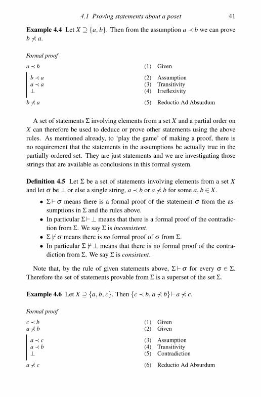
4.1 Proving statements about a poset 41
Example 4.4 Let X ⊇ {a, b}. Then from the assumption a ≺ b we can proveb �≺ a.
Formal proof
a ≺ b (1) Given
b ≺ a (2) Assumptiona ≺ a (3) Transitivity⊥ (4) Irreflexivity
b �≺ a (5) Reductio Ad Absurdum
A set of statements Σ involving elements from a set X and a partial order onX can therefore be used to deduce or prove other statements using the aboverules. As mentioned already, to ‘play the game’ of making a proof, there isno requirement that the statements in the assumptions be actually true in thepartially ordered set. They are just statements and we are investigating thosestrings that are available as conclusions in this formal system.
Definition 4.5 Let Σ be a set of statements involving elements from a set Xand let σ be ⊥ or else a single string, a ≺ b or a �≺ b for some a, b ∈ X .
• Σ�σ means there is a formal proof of the statement σ from the as-sumptions in Σ and the rules above.
• In particular Σ�⊥ means that there is a formal proof of the contradic-tion from Σ. We say Σ is inconsistent.
• Σ � �σ means there is no formal proof of σ from Σ.• In particular Σ � �⊥ means that there is no formal proof of the contra-
diction from Σ. We say Σ is consistent.
Note that, by the rule of given statements above, Σ� σ for every σ ∈ Σ.Therefore the set of statements provable from Σ is a superset of the set Σ.
Example 4.6 Let X ⊇ {a, b, c}. Then {c ≺ b, a �≺ b}�a �≺ c.
Formal proof
c ≺ b (1) Givena �≺ b (2) Given
a ≺ c (3) Assumptiona ≺ b (4) Transitivity⊥ (5) Contradiction
a �≺ c (6) Reductio Ad Absurdum
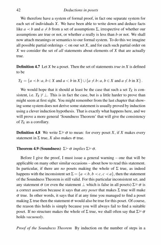
42 Deductions in posets
We therefore have a system of formal proof, in fact one separate system foreach set of individuals X . We have been able to write down and deduce factslike a ≺ b and a �≺ b from a set of assumptions Σ, irrespective of whether ourassumptions are true or not, or whether a really is less than b or not. We shallnow attach meanings or semantics to our formal system. To do this we imagineall possible partial orderings < on our set X , and for each such partial order onX we consider the set of all statements about elements of X that are actuallytrue.
Definition 4.7 Let X be a poset. Then the set of statements true in X is definedto be
TX = {a ≺ b : a, b ∈ X and a < b in X}∪{a �≺ b : a, b ∈ X and a �< b in X} .
We would hope that it should at least be the case that such a set TX is con-sistent, i.e. TX � �⊥. This is in fact the case, but is a little harder to prove thanmight seem at first sight. You might remember from the last chapter that show-ing some system does not derive some statement is usually proved by inductionusing a clever induction hypothesis. That is exactly what happens here, and wewill prove a more general ‘Soundness Theorem’ that will give the consistencyof TX as a corollary.
Definition 4.8 We write Σ � σ to mean: for every poset X , if X makes everystatement in Σ true, X also makes σ true.
Theorem 4.9 (Soundness) Σ�σ implies Σ�σ .
Before I give the proof, I must issue a general warning – one that will beapplicable on many other similar occasions – about how to read this statement.In particular, if there are no posets making the whole of Σ true, as indeedhappens with the inconsistent set Σ = {a ≺ b, b ≺ c, c ≺ a}, then the statementof the Soundness Theorem is still valid. For this particular inconsistent set, andany statement σ (or even the statement ⊥ which is false in all posets) Σ�σ isa correct assertion because it says that any poset that makes Σ true will makeσ true. In other words, it says that if at any time you managed to find a posetmaking Σ true then the statement σ would also be true for this poset. Of course,the reason this holds is simply because you will always fail to find a suitableposet. If no structure makes the whole of Σ true, we shall often say that Σ�σholds vacuously.
Proof of the Soundness Theorem By induction on the number of steps in a
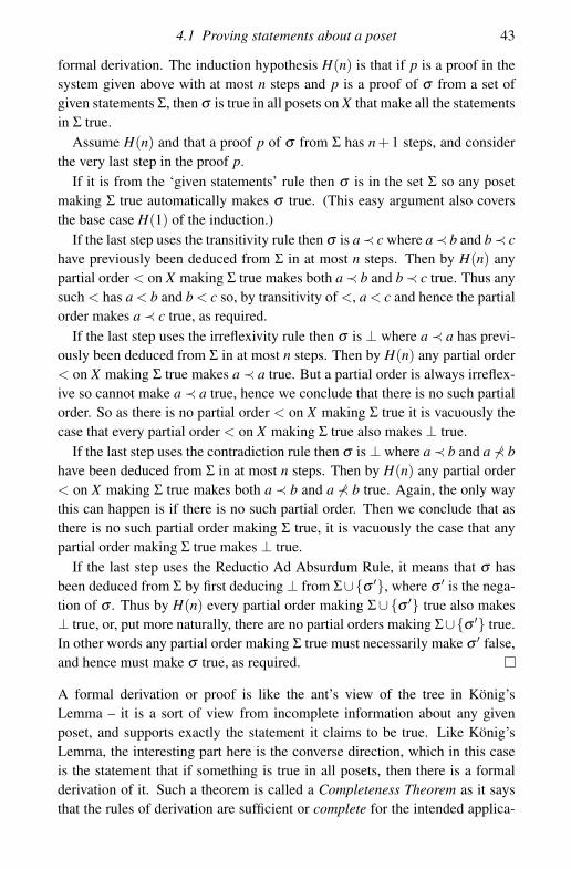
4.1 Proving statements about a poset 43
formal derivation. The induction hypothesis H(n) is that if p is a proof in thesystem given above with at most n steps and p is a proof of σ from a set ofgiven statements Σ, then σ is true in all posets on X that make all the statementsin Σ true.
Assume H(n) and that a proof p of σ from Σ has n + 1 steps, and considerthe very last step in the proof p.
If it is from the ‘given statements’ rule then σ is in the set Σ so any posetmaking Σ true automatically makes σ true. (This easy argument also coversthe base case H(1) of the induction.)
If the last step uses the transitivity rule then σ is a≺ c where a≺ b and b≺ chave previously been deduced from Σ in at most n steps. Then by H(n) anypartial order < on X making Σ true makes both a ≺ b and b ≺ c true. Thus anysuch < has a < b and b < c so, by transitivity of <, a < c and hence the partialorder makes a ≺ c true, as required.
If the last step uses the irreflexivity rule then σ is ⊥ where a ≺ a has previ-ously been deduced from Σ in at most n steps. Then by H(n) any partial order< on X making Σ true makes a ≺ a true. But a partial order is always irreflex-ive so cannot make a ≺ a true, hence we conclude that there is no such partialorder. So as there is no partial order < on X making Σ true it is vacuously thecase that every partial order < on X making Σ true also makes ⊥ true.
If the last step uses the contradiction rule then σ is ⊥ where a ≺ b and a �≺ bhave been deduced from Σ in at most n steps. Then by H(n) any partial order< on X making Σ true makes both a ≺ b and a �≺ b true. Again, the only waythis can happen is if there is no such partial order. Then we conclude that asthere is no such partial order making Σ true, it is vacuously the case that anypartial order making Σ true makes ⊥ true.
If the last step uses the Reductio Ad Absurdum Rule, it means that σ hasbeen deduced from Σ by first deducing ⊥ from Σ∪{σ ′}, where σ ′ is the nega-tion of σ . Thus by H(n) every partial order making Σ∪{σ ′} true also makes⊥ true, or, put more naturally, there are no partial orders making Σ∪{σ ′} true.In other words any partial order making Σ true must necessarily make σ ′ false,and hence must make σ true, as required.
A formal derivation or proof is like the ant’s view of the tree in Konig’sLemma – it is a sort of view from incomplete information about any givenposet, and supports exactly the statement it claims to be true. Like Konig’sLemma, the interesting part here is the converse direction, which in this caseis the statement that if something is true in all posets, then there is a formalderivation of it. Such a theorem is called a Completeness Theorem as it saysthat the rules of derivation are sufficient or complete for the intended applica-

44 Deductions in posets
tion. By switching the implication round to the contrapositive, completenesstheorems can also be seen as mathematical theorems that say certain mathe-matical structures exist, in this case, saying that certain order relations < exist.We are going to present our Completeness Theorem in this second form first.
Theorem 4.10 (Completeness) Suppose Σ is a consistent set of statementsabout elements of a set X. Then there is a partial order < on X making everystatement in Σ true.
Proof Define a partial order < on X by
a < b if and only if Σ�a ≺ b.
We need to prove that this is a partial order, and that all statements in Σ aremade true by this order.
To see that it is a partial order, we check the axioms. First if Σ� a ≺ b andΣ� b ≺ c then Σ� a ≺ c by the transitivity rule of deduction. So a < b andb < c imply a < c. For the irreflexivity axiom, consider a ∈ X . It cannot bethat Σ�a ≺ a, for this would imply Σ�⊥ by the irreflexivity rule of deduction,contradicting the consistency of Σ. Therefore Σ � �a ≺ a so by our definition itis not true that a < a.
To show that every statement in Σ is true for this order, suppose a statementof the form a ≺ b is in Σ. Then Σ� a ≺ b is immediate by the rule on givenstatements. If a �≺ b is in Σ then we need to show that Σ � �a ≺ b. (This requiresa little care: it is not the same thing as saying Σ� a �≺ b.) But suppose not,i.e. suppose Σ�a ≺ b. Then we already have a �≺ b ∈ Σ so from Σ�a �≺ b andthe contradiction rule we have Σ�⊥, which is impossible by the consistencyof Σ.
We already introduced a semantic notion of deduction, Σ � σ . This semanticdeduction is deduction from ‘total mathematical knowledge’. If we knew ev-erything there is to know about all possible orderings < on X we could decidequestions such as whether Σ�σ .
The Completeness Theorem, in its alternative form, says that anything thatmight have been deduced from ‘total mathematical knowledge’ by examiningall of the posets on X can in fact be deduced by a finite formal derivation. Inother words our rules of derivation are complete in the sense that they captureall possible (semantic) deductions.
Theorem 4.11 (Contrapositive of the Completeness Theorem) Suppose Xis a set, Σ is a set of statements about a partial order on X, and σ is a further

4.1 Proving statements about a poset 45
statement such that Σ�σ . Then there is a formal proof or derivation from therules given that Σ implies σ , i.e. Σ�σ .
Proof If not, Σ � �σ , so by the Reductio Ad Absurdum Rule, Σ∪{σ ′} is consis-tent, where σ ′ is the opposite, or negation, of σ . This is because if Σ∪{σ ′}�⊥then Σ�σ by Reductio Ad Absurdum. It follows that by the first form of theCompleteness Theorem there would be a partial order < on X making Σ trueand σ false, contradicting the assumption Σ�σ .
The reader should note in the proof of the theorem just given the example ofan informal nested proof by contradiction, i.e. one argument by contradictioninside another.
Notice also that the Soundness Theorem as originally stated is the exactconverse of this. It says that Σ�σ implies Σ�σ .
We have now proved our Completeness and Soundness Theorems for thissystem. But so far in this chapter, despite the new notation and definitions andcare required in separating the objects of discussion (formal derivations) fromour proofs about them, the mathematics has been comparatively straightfor-ward and no particularly interesting mathematical results have been proved.This changes with the next theorem, which relies on the following definitionand lemma.
Definition 4.12 Say a statement is positive if it is of the form a ≺ b andnegative if it is of the form a �≺ b.
Lemma 4.13 Suppose X is a non-empty set, and Σ is a consistent set of positivestatements about a partial order on the elements of X. Suppose a, b are inX and are distinct. Then either Σ∪ {a ≺ b} is consistent or Σ∪ {b ≺ a} isconsistent.
Proof Let us suppose that Σ∪{b ≺ a} is not consistent, so by the ReductioAd Absurdum Rule Σ� b �≺ a. Then by the Completeness Theorem and theconsistency of Σ there is a partial order < on X making Σ true, and by theSoundness Theorem the order < must also make b �≺ a.
We now define a new order � on X as follows:
x � y if and only if either x < y or both x � a and b � y.
We need to show that this is a poset that makes all of Σ true and also makesa ≺ b true.
To check transitivity, suppose that x � y � z. There are several cases.
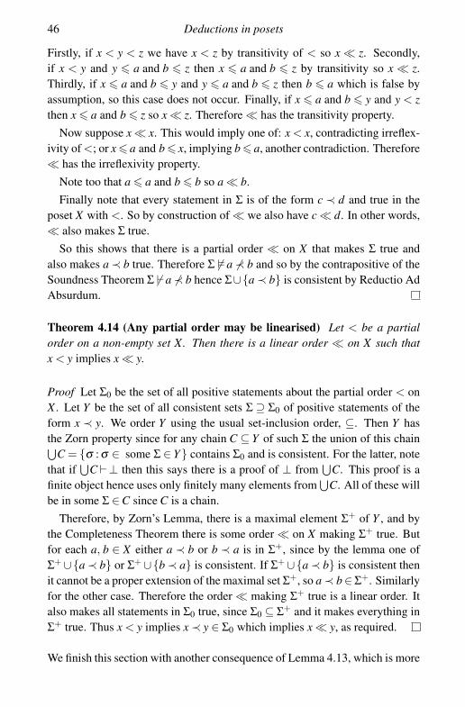
46 Deductions in posets
Firstly, if x < y < z we have x < z by transitivity of < so x � z. Secondly,if x < y and y � a and b � z then x � a and b � z by transitivity so x � z.Thirdly, if x � a and b � y and y � a and b � z then b � a which is false byassumption, so this case does not occur. Finally, if x � a and b � y and y < zthen x � a and b � z so x � z. Therefore � has the transitivity property.
Now suppose x � x. This would imply one of: x < x, contradicting irreflex-ivity of <; or x � a and b � x, implying b � a, another contradiction. Therefore� has the irreflexivity property.
Note too that a � a and b � b so a � b.Finally note that every statement in Σ is of the form c ≺ d and true in the
poset X with <. So by construction of � we also have c � d. In other words,� also makes Σ true.
So this shows that there is a partial order � on X that makes Σ true andalso makes a ≺ b true. Therefore Σ ��a �≺ b and so by the contrapositive of theSoundness Theorem Σ � �a �≺ b hence Σ∪{a ≺ b} is consistent by Reductio AdAbsurdum.
Theorem 4.14 (Any partial order may be linearised) Let < be a partialorder on a non-empty set X. Then there is a linear order � on X such thatx < y implies x � y.
Proof Let Σ0 be the set of all positive statements about the partial order < onX . Let Y be the set of all consistent sets Σ ⊇ Σ0 of positive statements of theform x ≺ y. We order Y using the usual set-inclusion order, ⊆. Then Y hasthe Zorn property since for any chain C ⊆ Y of such Σ the union of this chain⋃
C = {σ : σ ∈ some Σ ∈ Y} contains Σ0 and is consistent. For the latter, notethat if
⋃C�⊥ then this says there is a proof of ⊥ from
⋃C. This proof is a
finite object hence uses only finitely many elements from⋃
C. All of these willbe in some Σ ∈C since C is a chain.
Therefore, by Zorn’s Lemma, there is a maximal element Σ+ of Y , and bythe Completeness Theorem there is some order � on X making Σ+ true. Butfor each a, b ∈ X either a ≺ b or b ≺ a is in Σ+, since by the lemma one ofΣ+∪{a ≺ b} or Σ+∪{b ≺ a} is consistent. If Σ+∪{a ≺ b} is consistent thenit cannot be a proper extension of the maximal set Σ+, so a ≺ b∈Σ+. Similarlyfor the other case. Therefore the order � making Σ+ true is a linear order. Italso makes all statements in Σ0 true, since Σ0 ⊆ Σ+ and it makes everything inΣ+ true. Thus x < y implies x ≺ y ∈ Σ0 which implies x � y, as required.
We finish this section with another consequence of Lemma 4.13, which is more

4.2 Examples and exercises 47
‘logical’ in nature. A general theme in many parts of logic is as follows: be-cause formal proofs are rather special and difficult to come by, we should feelthat having a proof of a statement is often mathematically rather stronger thanjust knowing that the statement is true. This is similar to the fact that knowinga particular infinite path in a tree is often more useful than simply knowingthat the tree is infinite. This observation is particularly relevant when the state-ment is provable from some ‘weakened’ form of the system, since one thenhas to work even harder to get the formal proof. If this intuition is correct,there should be some nice mathematical consequences when we know a for-mal proof exists, rather than just knowing the statement is true, and sometimesthe proof itself can be converted to a proof of something better.
Our last result in this section is a rather pretty illustration of exactly this sit-uation. It says that if a negative statement can be proved from a set of positivestatements then there is a stronger positive statement we could have provedinstead. Of course this only works for the particular system of this chapter,and the reason it works is Lemma 4.13. The proof uses both Soundness andCompleteness Theorems.
Theorem 4.15 If Σ is a set of positive statements about a partial order < on aset X and a, b ∈ X are distinct, then Σ�b �≺ a implies that Σ�a ≺ b.
Proof We show the contrapositive, that Σ � �a ≺ b implies Σ � �b �≺ a.Suppose Σ � � a ≺ b. Then Σ∪{a �≺ b} ��⊥ by the Reductio Ad Absurdum
Rule. So by the Completeness Theorem there is a partial order on X makingΣ and a �≺ b true. By the proof of Lemma 4.13, this shows that there is apartial order � on X making Σ true and also making b ≺ a true. Hence by theSoundness Theorem Σ∪{b ≺ a} ��⊥ and Σ � �b �≺ a by the contradiction rule,as if Σ�b �≺ a then Σ∪{b ≺ a}�⊥.
Of course, no such result can hold without some special condition on Σ suchas it being a set of positive statements. Indeed {b �≺ a}� b �≺ a always holds,but {b �≺ a} ��a ≺ b.
4.2 Examples and exercises
We have introduced a lot of notation and terminology in this chapter, and someof it is quite tricky to master at first. For example, there is a big differencebetween Σ � �a ≺ b and Σ�a �≺ b. Some of the arguments employed are a littlesubtle too, with uses of contrapositive statements and also uses of informal

48 Deductions in posets
proofs by contradiction within a larger argument. Some of the exercises hereinvestigate these areas further.
The main point of the chapter is to illustrate the key methods of logic, offormal systems and semantics, applied to a familiar situation. Once again,the fact that proofs are finite objects is used in several places, for example toshow that a poset of a consistent set of sentences has the Zorn property (in theproof of the theorem that any partial order may be linearised). The techniqueof switching between the point-of-view of formal proofs, or �, and what theseformal proofs mean, or �, using the Completeness and Soundness Theoremsgives useful and interesting mathematical information.
Exercise 4.16 Show that ∅�{a �≺ a}.
Exercise 4.17 Show that:
(i) {a ≺ b, b �≺ c} ��a �≺ c(ii) {a �≺ b, b ≺ c} ��a �≺ c
(iii) {a �≺ b, b �≺ c} ��a �≺ c
(Hint: use soundness.)
Exercise 4.18 Explain the difference between the two statements Σ � � a ≺ band Σ�a �≺ b. Does either one of these imply the other? Justify your answer.
Exercise 4.19 Suppose Σ is a consistent set of statements about elements of aset X , and a, b ∈ X . Prove that either Σ∪{a ≺ b} is consistent or Σ∪{a �≺ b}is consistent.
Exercise 4.20 Suppose Σ is a set of negative statements (i.e. of statements ofthe form a �≺ b for a, b ∈ X) and suppose σ is positive. Show that Σ � �σ .
The proof we gave of the Completeness Theorem (Theorem 4.10) was ratherspecialised to partial orders and does not generalise nicely to other systems.The following exercise gives an alternative.
Exercise 4.21 Suppose Σ is a consistent set of statements about elements ofa set X . Show that there is Σ+ ⊇ Σ which is maximal in X = {Γ ⊇ Σ : Γ � �⊥},where Γ ranges over all sets of statements of the form a ≺ b or a �≺ b aboutelements of X . Define < on X by a < b if and only if Σ+�a ≺ b. Show that <
is a partial order on X such that Σ+ is precisely the set of statements true for <.
To illustrate this, the following exercise discusses a modification of our sys-tem to allow for deductions about linear orders.

4.3 Linearly ordering algebraic structures* 49
Exercise 4.22 Add a new rule to the system that says, if a, b are distinctelements of X such that the statement a �≺ b has been deduced, then b ≺ a mayalso be deduced. Also, redefine Σ�σ to mean every linear order making Σ truemust make σ true. State and prove Completeness and Soundness Theorems forthis system. (Hint: for the proof of a Completeness Theorem, follow the ideaof the previous exercise.)
Similar systems can describe preorders and equivalence relations, as the nexttwo exercises show.
Exercise 4.23 Let X be a set with at least two elements. Consider the followingformal system, where statements are allowed to be of the form a � b wherea, b ∈ X .
The rules of deduction are: (1) the ‘given statements rule’ above; (2) for ana ∈ X the statement a � a can be deduced; and (3) if a � b and b � c have beendeduced where a, b, c ∈ X then we may deduce a � c.
Prove the following Soundness Theorem that if Σ� a � b then a � b holdsin any preorder on X that makes Σ true. Prove also that ‘Σ� a � b’ defines apreorder on X that makes Σ true.
Exercise 4.24 Develop a formal system for proofs about an equivalence re-lation ∼ on a set X . Prove Soundness and Completeness Theorems for yoursystem.
4.3 Linearly ordering algebraic structures*
In general, the notion of formal proof and the Completeness Theorem can beregarded as a clever way of organising a poset with the Zorn property andthe consequences of having maximal elements. So in principle, the logicaltechniques described in this book can be avoided. That said, in many real-lifesituations the correct notion of consistency required is so complicated that itseems humanly impossible to avoid some of the logical manoeuvres describedin later chapters.
Exercise 4.25 Prove the theorem that any partial order can be linearised byusing Zorn’s Lemma directly.
As an astute reader will have observed, some of the results in this chaptercan be proved without the use of the Axiom of Choice, including (unusually)the Completeness Theorem. On the other hand, the theorem that any partialorder can be linearised requires some Choice, but it turns out that it is not

50 Deductions in posets
equivalent to the full Axiom of Choice. In the rest of this section we shall lookat other examples where these systems of proof can help organise and provesome results in algebra related to ordered structures; all of these will requireZorn’s Lemma or the Axiom of Choice in some way.
We start with abelian groups. Recall that an abelian group is a group G withbinary operation + and identity 0 for which the operation is commutative:x+ y = y+ x for all x, y ∈ G. We write nx for x+ x+ · · ·+ x where x appears ntimes.
Definition 4.26 An ordered abelian group is an abelian group G with a linearorder < on G such that
x < y implies x+ z < y+ z
for all x, y, z ∈ G.An abelian group G is orderable if there is some linear order < on G making
G into an ordered abelian group.
For example, the group (Z, +) is orderable, and in fact the usual ordersatisfies the axiom above. On the other hand, no finite cyclic group is or-derable since if x is a generator and 0 < x then the axiom above implies0 < x < x + x < x + x + x < · · · but nx = x + · · ·+ x = 0 where n is the or-der of x. This contradicts transitivity of <. A similar argument applies whenx < 0.
Definition 4.27 An element x of an abelian group G is torsion if x �= 0 andthere is n > 0 in N such that nx = 0. A group G is torsion-free if there are notorsion elements of G other than the identity element, 0.
Exercise 4.28 Continue the argument for finite cyclic groups above, showingthat an abelian group with a torsion element x is not orderable.
We want to investigate which abelian groups are orderable. The first step isto extend the system of Exercise 4.22 and prove Completeness and SoundnessTheorems.
Let our set X of elements be the elements of G, an abelian group. Add a newrule to the system for linear orders in Exercise 4.22 that says that if a, b, c ∈ Xand a ≺ b has been deduced then a′ ≺ b′ may be deduced, where a′ = a + cand b′ = b+ c.
Exercise 4.29 Prove that Σ � � ⊥ if and only if G is orderable with a linearorder < making all statements in Σ true; in particular ∅ � �⊥ if and only if G is

4.3 Linearly ordering algebraic structures* 51
orderable. (For completeness, use a Zorn’s Lemma argument similar to that inExercise 4.21.)
The next stage is to simplify this proof system so that we can analyse italgebraically. Using the group operation we can rewrite the statement a ≺ bas 0 ≺ c where c = b−a ∈ G. Because our orders will be linear, a �≺ b is ‘thesame as’ b ≺ a for a �= b, and we will have no need for negative statements.So the new simplified system will have statements ⊥ and 0 ≺ a for a ∈ G only.The new proof rules will be:
• the Given Statements Rule;• the rule, from 0 ≺ 0 deduce ⊥;• the rule, from 0 ≺ a and 0 ≺ b deduce 0 ≺ c, where c = a+b;• the Reductio Ad Absurdum Rule in the form, if from assumption 0 ≺ a
(where a �= 0) you can prove ⊥, then you may deduce 0 ≺ b withoutany assumptions, where b = −a is the inverse of a.
Note that the new Reductio Ad Absurdum Rule combines the old Reductio AdAbsurdum Rule with the rule for linearity of the order. The rule about a+b isa special case of the rule about the order respecting addition in the group.
We could prove new Completeness and Soundness Theorems for the newsimplified system directly. However, in this case there is a simpler alternative:to define a translation of one system into the other.
Definition 4.30 We define a translation t of the system of Exercise 4.29 intothe new system by letting the translation t(⊥) of ⊥ be ⊥, t(a ≺ b) be 0 ≺ b−a,and for a �= b, we let t(a �≺ b) be 0 ≺ a−b. (For a = b the statement a �≺ b isalways provable and may be safely ignored.)
Exercise 4.31 Prove by induction on proofs that a ≺ b is provable in the firstsystem from Σ implies that t(a ≺ b) is provable in the simplified system from{t(σ) : σ ∈ Σ}. Also, arguing directly this time, prove a converse to this state-ment.
Hence deduce Completeness and Soundness Theorems for the new system,including the statement that Σ � � ⊥ if and only if the group G is orderable insuch a way that every statement in Σ is true for the new order on G.
We are now in a position to prove our converse to Exercise 4.28 and provethat every torsion-free abelian group is orderable. The main technical result(giving the induction on length of proofs that is required) is the following.
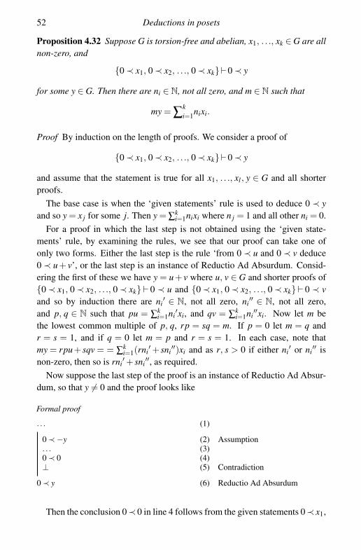
52 Deductions in posets
Proposition 4.32 Suppose G is torsion-free and abelian, x1, . . ., xk ∈ G are allnon-zero, and
{0 ≺ x1, 0 ≺ x2, . . ., 0 ≺ xk}�0 ≺ y
for some y ∈ G. Then there are ni ∈ N, not all zero, and m ∈ N such that
my = ∑ki=1nixi.
Proof By induction on the length of proofs. We consider a proof of
{0 ≺ x1, 0 ≺ x2, . . ., 0 ≺ xk}�0 ≺ y
and assume that the statement is true for all x1, . . ., xl , y ∈ G and all shorterproofs.
The base case is when the ‘given statements’ rule is used to deduce 0 ≺ yand so y = x j for some j. Then y = ∑k
i=1nixi where n j = 1 and all other ni = 0.For a proof in which the last step is not obtained using the ‘given state-
ments’ rule, by examining the rules, we see that our proof can take one ofonly two forms. Either the last step is the rule ‘from 0 ≺ u and 0 ≺ v deduce0 ≺ u + v’, or the last step is an instance of Reductio Ad Absurdum. Consid-ering the first of these we have y = u+ v where u, v ∈ G and shorter proofs of{0 ≺ x1, 0 ≺ x2, . . ., 0 ≺ xk} � 0 ≺ u and {0 ≺ x1, 0 ≺ x2, . . ., 0 ≺ xk} � 0 ≺ vand so by induction there are ni
′ ∈ N, not all zero, ni′′ ∈ N, not all zero,
and p, q ∈ N such that pu = ∑ki=1ni
′xi, and qv = ∑ki=1ni
′′xi. Now let m bethe lowest common multiple of p, q, rp = sq = m. If p = 0 let m = q andr = s = 1, and if q = 0 let m = p and r = s = 1. In each case, note thatmy = rpu+ sqv = = ∑k
i=1(rni′ + sni
′′)xi and as r, s > 0 if either ni′ or ni
′′ isnon-zero, then so is rni
′ + sni′′, as required.
Now suppose the last step of the proof is an instance of Reductio Ad Absur-dum, so that y �= 0 and the proof looks like
Formal proof
. . . (1)
0 ≺−y (2) Assumption. . . (3)0 ≺ 0 (4)⊥ (5) Contradiction
0 ≺ y (6) Reductio Ad Absurdum
Then the conclusion 0≺ 0 in line 4 follows from the given statements 0≺ x1,

4.3 Linearly ordering algebraic structures* 53
0 ≺ x2, . . . , 0 ≺ xk and the additional assumption 0 ≺ −y, and thus by ourinduction hypothesis there are m, ni ∈ N (not all zero) such that
0 = m(−y)+∑ki=1nixi.
Now y �= 0 (otherwise the assumption to the Reductio Ad Absurdum Rule isnot allowed) so if all of the ni are zero we would have my = 0 contradicting thefact that G is torsion-free. Thus at least one of the ni is non-zero and
my = ∑ki=1nixi
as required.
Corollary 4.33 Let G be torsion-free and abelian. Then G is orderable.
Proof If not then ⊥ is provable from no given statements. Without any state-ments previously given the first step must be a subproof with some assumption0 ≺ y (y �= 0), and the conclusion to this subproof is the contradiction 0 ≺ 0.Thus by the proposition 0 = ny for some n ∈ N, n not zero. Thus G is nottorsion-free.
We now turn, briefly, to non-abelian groups, i.e. groups where the commutativ-ity axioms might fail. As is conventional, we revert to multiplicative notation.Since the group may no longer be abelian we must specify the side that theaction in the axiom ‘a < b implies ac < bc’ takes place.
Definition 4.34 A right-ordered group is a group G with a linear order < onG such that a < b implies ac < bc for all a, b, c ∈ G. A right-orderable groupis a group G which may be made into a right-ordered group by the choice ofan appropriate order.
It is not so easy to give a purely algebraic criterion that describes when agroup G can be ordered in such a way that it becomes a right-ordered group.However, the analogue of Exercise 4.29 holds.
Exercise 4.35 Let X be the set of elements of a group G. Add a new rule to thesystem for linear orders in Exercise 4.22 that says that if a, b, c ∈ X and a ≺ bhas been deduced then a′ ≺ b′ may be deduced, where a′ = ac and b′ = bc.Prove that Σ � � ⊥ if and only if there is a linear order on X making G intoa right-ordered group in which all statements in Σ are true, and in particular∅ � �⊥ if and only if G is right-orderable.

54 Deductions in posets
The following exercise gives a family of examples that are right-orderable.In attempting it, it may be helpful to know that any set such as Ω has a well-order, i.e. a linear order in which every non-empty subset has a least element.(This fact about well-orders can be proved from Zorn’s Lemma and is in factequivalent to the Axiom of Choice.)
Exercise 4.36 Let G be a group of permutations of a linearly ordered setΩ, i.e. each g ∈ G is a bijection g: Ω→Ω, with the group operation beingcomposition of maps. The order on Ω will be denoted �. Suppose each g ∈ Grespects � in the sense that x � y implies g(x)� g(y) for each x, y∈Ω. Showthat G is right-orderable.
The ‘simplified system’ for orderable abelian groups that we looked at aboveconcerns specifications of which elements are positive, i.e. for which a we have0 < a. A related result on orderability of fields goes via specifying the positiveelements in a field.
Definition 4.37 A field F is an ordered field if it has a linear order < such thatx < y implies x + z = y + z for all x, y, z ∈ F and x < y implies xz = yz for allpositive x, y, z ∈ F . The field F is orderable or formally real if there is such anorder that can be defined on F .
Definition 4.38 Let F be a field. A pre-positive cone of F is a set P ⊆ F whichis closed under addition and multiplication, contains 1 but does not contain 0,and contains all x2 for x �= 0 in F . A positive cone of F is a maximal pre-positive cone P ⊆ F .
Exercise 4.39 Use Zorn’s Lemma to show that a pre-positive cone of a field Fis always contained in a positive cone.
Exercise 4.40 Let P be a positive cone of F . Define < by x < y if and onlyif y− x ∈ P. Show that this defines a linear order on F that makes F into aordered field.
Exercise 4.41 Deduce that F is orderable if and only if F has a pre-positivecone, and that this is the case if and only if no finite sum of non-zero squaresfrom F equals −1.
Exercise 4.42 Reinterpret these results as a formal system, proving Soundnessand Completeness Theorems for your system.

5
Boolean algebras
5.1 Boolean algebras
Partially ordered and linearly ordered sets may be interesting but they are notreally ‘logic’ in the usual sense of the word: they do not represent logical state-ments nor do they model logical operations such as ‘not’, ‘and’, or ‘or’. Weare now going to investigate special kinds of posets called boolean algebras,the elements of which can be used to represent logical propositions.
We start by adding extra operations such as ‘and’, ‘or’, and ‘not’ to a poset,turning it into a boolean algebra. (But it turns out that it is much more con-venient to look at non-strict posets with an order relation �, though you maytake a strict partial order and change it to a non-strict order as explained be-fore.) The axioms for a boolean algebra are given in three groups, making upthe axioms for a lattice, a distributive lattice and a boolean algebra proper. Wegive each group separately.
Definition 5.1 A lattice is a poset X with non-strict order � such that everypair of elements x, y of X has a greatest lower bound denoted inf(x, y) or x∧ ysatisfying
x∧ y � x and x∧ y � y
and also
z � x and z � y imply z � x∧ y
for all z ∈ X ; furthermore, every pair of elements x, y of X has a least upperbound denoted sup(x, y) or x∨ y satisfying
x∨ y � x and x∨ y � y
and also
z � x and z � y imply z � x∨ y
55

56 Boolean algebras
for all z ∈ X .
Exercise 5.2 Let X be a poset. Suppose a, b ∈ X are both greatest lowerbounds of x, y ∈ X , i.e. suppose that a � x, a � y, b � x and b � y (so botha, b are lower bounds of x, y) and that whenever z satisfies z � x and z � y thenz � a and z � b (so both a, b are greatest lower bounds of x, y). Show that a = b.Thus there can be at most one greatest lower bound x∧y of x, y ∈ X . Similarly,show that there can be at most one least upper bound x∨ y of x, y ∈ X .
Exercise 5.3 Show that any linearly ordered set is a lattice.
Exercise 5.4 Show that any finite poset is a lattice.
Exercise 5.5 Find an infinite poset which is not a lattice.
Definition 5.6 A distributive lattice is a lattice X such that the distributivityaxioms hold for ∧ and ∨, i.e.
x∧ (y∨ z) = (x∧ y)∨ (x∧ z)
and
x∨ (y∧ z) = (x∨ y)∧ (x∨ z)
for all x, y ∈ X .
Example 5.7 If X is an infinite set, the set F of all finite subsets of X forms adistributive lattice under ⊆.
Example 5.8 Let A = {0, 1, 2, 3, 4} be the poset where 0 < 1 < 2 < 4, 0 <
3 < 4 and no other relations between these elements hold. Then A is a non-distributive lattice. (Exercise: compute 1∧ (2∨3) and (1∧2)∨ (1∧3) in A.)
Example 5.9 Let B = {0, 1, 2, 3, 4} be the poset where 0 < 1 < 4, 0 < 2 < 4,0 < 3 < 4 and no other relations hold. Then B is also a non-distributive lattice.(Exercise: compute 1∧ (2∨3) and (1∧2)∨ (1∧3) in B.)
Remark 5.10 The last two examples are typical of non-distributive lattices: infact, every non-distributive lattice contains a copy of either A of Example 5.8or B of Example 5.9. An ambitious reader might try to prove this as a moredifficult exercise.
Definition 5.11 A boolean algebra is a distributive lattice X containing two
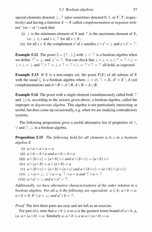
5.1 Boolean algebras 57
special elements denoted ⊥, � (also sometimes denoted 0, 1, or F , T , respec-tively) and having a function X →X called complementation or negation writ-ten ′ (or ¬ or c) such that:
(i) ⊥ is the minimum element of X and � is the maximum element of X ,i.e. ⊥ � x and x � � for all x ∈ X ;
(ii) for all x ∈ X the complement x′ of x satisfies x∧x′ = ⊥ and x∨x′ = �.
Example 5.12 The poset 2 = {�, ⊥} with ⊥ < � is a boolean algebra whenwe define �′ =⊥, and ⊥′ =�. You can check that ⊥∧⊥=⊥∧�=�∧⊥=⊥∨⊥ = ⊥ and �∧� = ⊥∨� = �∨⊥ = �∨� = � all hold, as expected.
Example 5.13 If X is a non-empty set, the poset P(X) of all subsets of Xwith the usual ⊆ is a boolean algebra where ⊥ = ∅, � = X , A′ = X \ A (setcomplementation) and A∧B = A∩B, A∨B = A∪B.
Example 5.14 The poset with a single element (simultaneously called both �and ⊥) is, according to the axioms given above, a boolean algebra, called theimproper or degenerate algebra. This algebra is not particularly interesting oruseful, but does come up occasionally, e.g. when we are studying contradictorysystems.
The following proposition gives a useful alternative list of properties of ∧,∨ and �, ⊥ in a boolean algebra.
Proposition 5.15 The following hold for all elements a, b, c in a booleanalgebra X
(i) a∧a = a∨a = a(ii) a∧b = b∧a and a∨b = b∨a
(iii) a∧ (b∧ c) = (a∧b)∧ c and a∨ (b∨ c) = (a∨b)∨ c(iv) a∧ (a∨b) = a∨ (a∧b) = a(v) a∧ (b∨ c) = (a∧b)∨ (a∧ c) and a∨ (b∧ c) = (a∨b)∧ (a∨ c)
(vi) ⊥∧a = ⊥, ⊥∨a = a, �∧a = a and �∨a = �(vii) a∧a′ = ⊥ and a∨a′ = �.
Additionally, we have alternative characterisations of the order relation in aboolean algebra. For all a, b the following are equivalent: a � b; a∧ b = a;a∨b = b; b′ ∧a = ⊥; and a′ ∨b = �.
Proof The first three parts are easy and are left as an exercise.For part (iv), note that a∨b � a so a is the greatest lower bound of a∨b, a,
i.e. a∧ (a∨b) = a. Similarly a, a∧b � a so a∨ (a∧b) = a.

58 Boolean algebras
The distributivity laws were already given as axioms of boolean algebras sothere is nothing to prove in the next point.
Since ⊥ is the least element, it must be the greatest lower bound of itself andany other a ∈ X . Hence ⊥∧a = ⊥. The other three equations in this group aresimilar.
The statements a∧ a′ = ⊥ and a∨ a′ = � were also given as axioms forboolean algebras.
If a � b then a is a lower bound for b and hence the greatest lower bound fora, b together. Conversely if a∧ b = a then a is a lower bound for b so a � b.The next case is similar. If a′ ∨b = � then doing ‘a∧’ to both sides and usingdistributivity we have the left hand side is equal to
a∧ (a′ ∨b) = (a∧a′)∨ (a∧b) = ⊥∨ (a∧b) = a∧b
and this equals the right hand side, which is a∧�= a, so a∧b = a. Converselydoing ‘a′∨’ to both sides of a∧b = a and using distributivity gives a′ ∨b = �.The other case is similar.
The last part of this proposition shows that the order relation in a boolean alge-bra can be defined in terms of ∧ or ∨. This gives us another way of specifying aboolean algebra as an algebraic structure somewhat like a ring, with operations∧, ∨ , ′ and elements �, ⊥ and defining � from these.
Proposition 5.16 Let (X , ∧, ∨, ′, �, ⊥) be an algebraic structure satisfyingproperties (i)–(vii) in Proposition 5.15 for all a, b, c ∈ X. Define � on X byany of the clauses given in the last part of the proposition. Then this makesX into a boolean algebra, with the sup and inf operations being ∨ and ∧, andwith maximum and minimum elements � and ⊥.
Proof It is necessary to check that � is a partial order satisfying the axioms inDefinition 5.11. Left as an exercise.
We can thus swap between our view of a boolean algebra as a poset or as analgebraic object like a ring at will, just like we swap between our views of astrict and non-strict poset.
Purists would read �, ⊥ as ‘top’ and ‘bottom’, respectively, and ∧, ∨ as‘meet’ and ‘join’. However, the symbols �, ⊥ are often read as ‘true’ and‘false’, and ∧, ∨ as ‘and’ and ‘or’. ‘Or’ is always inclusive or, i.e. meaningone or the other or both. The complementation operation is ‘not’, especiallywhen it is written as ¬.
The mathematically rather common implication, ‘if a then b’, often causes

5.1 Boolean algebras 59
some consternation, since from the point of view of natural language we nor-mally expect this to be true only when a and b have something to do with eachother. (So ‘if the sky has dark clouds then it will rain’ seems quite reason-able, but ‘if there are small green men on Mars then it is raining’ seems as ifit should be false, because what have the strange creatures on Mars got to dowith our rain? But on the other hand, if it really is raining, surely the statementis true whatever might be on Mars? And, if there are no small green men onMars, is the statement not vacuously true anyway?) There is no mathematicalsymbol that captures exactly this ‘natural’ idea of ‘if a then b’ where a shouldbe relevant to b, but the � in the boolean algebra does quite a good job in allother respects. Think of a � b as saying that b is at least as true as a. Thena � b is quite a good mathematical definition for ‘if a then b’, even if it doesnot capture all the nuances of natural language.
By the last part of Proposition 5.15, a � b is equivalent in a boolean algebrato the statement that a′ ∨b = �, or in words ‘not-a or b’.
We investigate this order relation as ‘implies’ or ‘if. . . then. . . ’ in the nextfew propositions. The first of these says that if a implies b then a and c impliesb and c, and with something similar for ‘or’.
Proposition 5.17 Let B be a boolean algebra with a, b, c ∈ B and a � b. Thena∧ c � b∧ c and a∨ c � b∨ c.
Proof For a∧c � b∧c it suffices to observe that a∧c � a � b and a∧c � c soa∧ c is a lower bound of both b, c hence is less than or equal to the least suchlower bound.
For a∨ c � b∨ c argue similarly using a � b � b∨ c and c � b∨ c.
The next proposition is the law of contraposition: the contrapositive of ‘a im-plies b’ is ‘not-b implies not-a’. As shown here, an implication and its contra-positive are equivalent.
Proposition 5.18 Let B be a boolean algebra and suppose a � b. Then b′ � a′.
Proof If a � b then
b′ = b′ ∧ (a′ ∨a) � b′ ∧ (a′ ∨b) = (b′ ∧a′)∨ (b∧b′) = b′ ∧a′
so b′ � a′.
Proposition 5.19 Let B be a boolean algebra and suppose b′ � a′. Then a � b.

60 Boolean algebras
Proof Exercise, to be done in a similar way. Or use the previous result andProposition 5.22 on Uniqueness of Complements below, where it is shown thatx′′ = x in any boolean algebra B.
The next proposition is often useful. It says that to determine whether a state-ment a holds it suffices to consider two cases: one where b is true, and onewhere it is false. Of course b can be any proposition at all. (It can even be aitself, in which case the proposition would be a triviality.)
Proposition 5.20 Let B be a boolean algebra and suppose a, b ∈ B. Then(a∧b)∨ (a∧b′) = a.
Proof By the distributivity laws,
(a∧b)∨ (a∧b′) = a∧ (b∨b′) = a∧� = a
as required.
There is a similar dual statement, with ‘and’ and ‘or’ swapped over.
Proposition 5.21 Let B be a boolean algebra and suppose a, b ∈ B. Then(a∨b)∧ (a∨b′) = a.
Proof Exercise.
Finally, we have an important result concerning ‘not’.
Proposition 5.22 (Uniqueness of Complements) Let B be a boolean algebra,with a, b ∈ B, and suppose that a∧ b = ⊥ and a∨ b = �. Then b = a′. Inparticular x′′ = x for all x ∈ B.
Proof Assume that a∧b = ⊥ and a∨b = �. Then
a′ = a′ ∨⊥ = a′ ∨ (a∧b) = (a′ ∨a)∧ (a′ ∨b) = �∧ (a′ ∨b) = a′ ∨b
by distributivity, so a′ � b, and similarly
a′ = a′ ∧� = a′ ∧ (a∨b) = (a′ ∧a)∨ (a′ ∧b) = ⊥∨ (a′ ∧b) = a′ ∧b
so a′ � b. Hence a′ = b.Now let a in the previous paragraph be x′, and put b = x. Then x′ ∧ b = ⊥
and x′ ∨b = �, hence b = x′′.

5.2 Examples and exercises 61
5.2 Examples and exercises
Exercise 5.23 Carry out the procedure that starts with a boolean algebra asan algebraic structure (X , ∧, ∨, ′, �, ⊥) satisfying the statements in Proposi-tion 5.15, defining an order relation by a � b if and only if a∧b = a and thenverifying that the poset obtained has the properties in Definition 5.11.
Exercise 5.24 Show that in any boolean algebra the expressions (a∧ b)′ and(a′ ∨b′) are equal.
Exercise 5.25 Let B be a boolean algebra. Show that the complementationoperation ′: B→B is one-to-one and onto.
Exercise 5.26 The following statements are all intuitively correct. (To verifythat they are valid, just multiply the first equation by 2 or 0.)
(a) 1 = 1 implies 2 = 2; (b) 1 = 2 implies 2 = 4; (c) 1 = 2 implies 0 = 0.On the other hand the following is not a correct implication:
(d) 1 = 1 implies 2 = 4.Assuming that a mathematical implication a implies b only depends on the
truth of a and b, and writing → for ‘implies’, deduce that mathematical im-plication should be fully determined by the following rules: (�→�) = �;(�→⊥) = ⊥; (⊥→�) = �; (⊥→�) = �.
5.3 Boolean algebra and the algebra of Boole*
The name ‘boolean algebra’ celebrates the contributions of George Boole tologic. In fact, Boole’s work is so important that the word ‘boolean’ has en-tered the language and is conventionally spelled without a capital letter. Boolewas the first to employ algebraic techniques in logic and is rightly commemo-rated for his contributions to logic, particularly in his books The MathematicalAnalysis of Logic (1847) and An Investigation of the Laws of Thought (1854).However, in keeping with the traditions of the time, Boole never wrote downa full set of axioms for his algebra, and it is not quite clear how one mightdescribe the algebra of Boole in modern terms.
Certainly the symbols ∧ and ∨ post-date Boole’s work by many years. Booleinstead used multiplication and addition operations, in what seems like a ring-like structure. It is commonly believed (especially by those who have not readBoole’s books) that Boole worked in what are now called boolean rings.

62 Boolean algebras
Definition 5.27 A boolean ring is a ring R which is commutative with 1 andfor which x2 = x for all x ∈ R.
Exercise 5.28 Given a boolean ring R, show that by defining a∧ b = ab anda∨b = ab+a(1−b)+(a−1)b on R, we obtain a boolean algebra.
Exercise 5.29 Given a boolean algebra, we can define a boolean ring on thesame set by ab = a∧b and a + b = (a∨b′)∧ (a′ ∨b). If this is applied to theboolean algebra resulting from the previous exercise we recover the originaladdition operation in R.
Exercise 5.30 Show that x + x = 0 holds for all x in a boolean ring R. Inparticular all boolean rings have characteristic 2, i.e. 1+1 = 0.
Exercise 5.31 Let R be a commutative ring with 1 and let I ⊆ R be the idealgenerated by all elements x(1−x) with x ∈ R. Show that R/I is a boolean ring,in fact the largest quotient of R which is a boolean ring.
The operations taking a boolean algebra to a boolean ring and back againdescribed in the last few exercises are inverse to each other. However, Boole’salgebra was not that of boolean rings, since (for example) there are a numberof places where he carefully includes a coefficient ‘2’ – indeed he sometimesdivides by 2 – and yet 1+1 = 0 holds in any boolean ring.
Instead, it seems that Boole’s algebra was of a ring R which is commutativeand has 1, in which there are no additive or multiplicative nilpotent elementsat all (meaning nx = x + x + · · ·+ x �= 0 for all n �= 0 and all x �= 0, and xn =xx· · ·x �= 0 for all n and all x �= 0), but some elements x of R have the (forthe time, counter-intuitive) property of being idempotent elements, i.e. x2 = x.Boole would call such x elective elements.
For an example of such a ring, consider a non-empty set X of individuals andconsider R to be the set of functions f : X →R with componentwise additionand multiplication, ( f + g)(x) = f (x) + g(x) and ( f g)(x) = f (x)g(x). Thenthe characteristic function of a subset A ⊆ R, defined by χA(x) = 1 if x ∈ Aand χA(x) = 0 otherwise, is idempotent and represents the set of individualsA. This particular ring can thus be seen to contain a representation of the setP(X) of all subsets of X and the idempotents in it are very closely related tothe boolean algebra P(X) with ⊆ , ∪ , ∩.
The mathematical part of Boole’s work in logic can be seen then to be aninvestigation into the properties of elective, or idempotent, elements of such aring R, and of functions of such elective arguments. In more modern terms, the
5.3 Boolean algebra and the algebra of Boole* 63
set E ⊆ R of electives or idempotents is not a subring of R, but may be madeinto a boolean ring by redefining the addition operation on it to be x⊕ y =x + y− 2xy. The development of boolean algebra from Boole’s algebra camesome time later.

6
Propositional logic
6.1 A system for proof about propositions
We are going to develop a formal system for proofs about boolean algebras,just as in a previous chapter we developed one for posets. It will also be richenough to simulate proofs in the systems given in Chapters 3 and 4, thoughwe will not be in a position to explain the precise connections until Chapter 7.(For this, please see Examples 7.27 and 7.29.)
The system will contain objects representing elements of a boolean algebrathat say things such as a � b and a = b, but there is a subtle and rather elegantpoint here: with our extra symbols for ∧, ∨ , ′, �, ⊥ we do not need to useeither of the symbols < or �, since a � b holds if and only if a′ ∨b = �. In-stead, the statements in our system will be elements of the boolean algebra – orrather terms representing elements in the boolean algebra – and if a statementis provable or derivable we shall think of it as being true, or equal to �.
The next definition explains the terms which will represent elements of someboolean algebra.
Definition 6.1 Let X be any set, which for this definition will be called a setof propositional letters. The set of boolean terms BT(X) over X is defined asa set of expressions, or strings of symbols, from a set of symbols including(, ), ∧ , ∨ , �, ⊥, ¬ and all elements of X , as follows.
• ⊥ and � are both boolean terms over X .• Any element a of X is a boolean term over X .• If t is a boolean term over X then so is ¬ t.• If t and s are boolean terms over X then so are (t ∧ s) and (t ∨ s).• No other object r is a boolean term unless it can be obtained by finitely
many applications of the previous four rules.
64

6.1 A system for proof about propositions 65
Example 6.2 If X = {a, b, c} then �, a, ((a∧¬b)∨ c), ((a∧¬b)∨ c), and¬⊥ are all distinct boolean terms over X .
Note that two terms such as � and ¬⊥, or (a∧ a) and (a∨ a), count asdistinct terms since they are different as strings of symbols, even though theywill evaluate to the same object in any boolean algebra.
Definition 6.3 Let X be a set, and let BT(X) be the set of boolean terms overX . A formal proof or derivation from assumptions Σ ⊆ BT(X) is a derivationof finite length where each statement in it is an element of BT(X) and whichuses only the following proof rules.
• (Given Statements Rule) Any σ ∈ Σ may be deduced from Σ in onestep.
• (Top Rule) The statement � may be deduced from any Σ in one step.• (∧-Introduction) If σ and τ have been derived from Σ then (σ ∧τ) may
be deduced from Σ in one further step.• (∨-Introduction) If τ has been deduced from Σ and σ ∈ BT(X) then
either of (σ ∨ τ), (τ ∨σ) may be deduced from Σ in one further step.• (∧-Elimination) If (σ ∧ τ) has been deduced from Σ then either σ or τ
may be deduced from Σ in one further step.• (∨-Elimination) If (σ ∨ τ) and ¬σ have been deduced from Σ then τ
may be deduced from Σ in one further step.• (¬-Elimination) If ¬¬σ has been deduced from Σ then σ may be de-
duced from Σ in one further step.• (Contradiction Rule) If σ and ¬σ have been deduced from Σ then ⊥
may be deduced from Σ in one further step.• (Reductio Ad Absurdum Rule) If ⊥ has been deduced from Σ∪{σ}
then ¬σ may be deduced from Σ in one further step.
The notation Σ�σ will be used as in previous chapters to mean that σ maybe deduced from Σ according to the rules above. Here, some set of proposi-tional letters X is understood and Σ ⊆ BT(X), σ ∈ BT(X). So Σ�σ meansthere is a formal proof, i.e. a finite structured list of statements and subproofsof BT(X) obeying the above rules, showing that σ can be deduced from as-sumptions from Σ. In particular we will say that Σ is inconsistent if Σ�⊥, andconsistent otherwise.
We shall give some examples of formal proofs here, and in so doing weshow how formal proofs are usually written, and spell out in more detail howthe above rules should be applied.
Example 6.4 Let X = {a, b} and Σ = {(¬a∨b)}. Then Σ�¬(a∧¬b).

66 Propositional logic
Formal proof
(a∧¬b) (1) Assumptiona (2) ∧-Elimination
¬a (3) Assumption⊥ (4) Contradiction
¬¬a (5) RAA¬b (6) ∧-Elimination(¬a∨b) (7) Given, from Σb (8) ∨-Elimination⊥ (9) Contradiction
¬(a∧¬b) (10) RAA
Example 6.5 Let X = {a, b}. Then ∅� (((a∧¬b)∨¬a)∨b).
Formal proof
¬(((a∧¬b)∨¬a)∨b) (1) Assumption
b (2) Assumption(((a∧¬b)∨¬a)∨b) (3) ∨-Introduction⊥ (4) Contradiction
¬b (5) RAA
¬a (6) Assumption((a∧¬b)∨¬a) (7) ∨-Introduction(((a∧¬b)∨¬a)∨b) (8) ∨-Introduction⊥ (9) Contradiction
¬¬a (10) RAAa (11) ¬-Elimination(a∧¬b) (12) ∧-Introduction((a∧¬b)∨¬a) (13) ∨-Introduction(((a∧¬b)∨¬a)∨b) (14) ∨-Introduction⊥ (15) Contradiction
¬¬(((a∧¬b)∨¬a)∨b) (16) RAA(((a∧¬b)∨¬a)∨b) (17) ¬-Elimination
This system is considerably more complicated than systems previously pre-sented in this book. It does, however, share many features with other systems.In particular, the derived objects in a proof are simply strings of symbols withno a priori meanings attached. (Though there is a clear idea that such ‘mean-ing’ should be connected with boolean algebras – this will be taken up in thenext chapter.) The proof rules are more complicated and there are more of
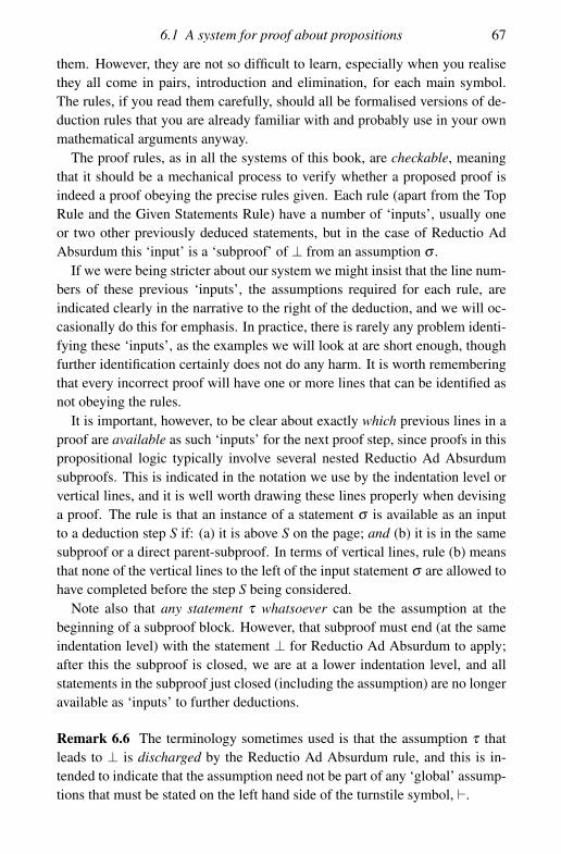
6.1 A system for proof about propositions 67
them. However, they are not so difficult to learn, especially when you realisethey all come in pairs, introduction and elimination, for each main symbol.The rules, if you read them carefully, should all be formalised versions of de-duction rules that you are already familiar with and probably use in your ownmathematical arguments anyway.
The proof rules, as in all the systems of this book, are checkable, meaningthat it should be a mechanical process to verify whether a proposed proof isindeed a proof obeying the precise rules given. Each rule (apart from the TopRule and the Given Statements Rule) have a number of ‘inputs’, usually oneor two other previously deduced statements, but in the case of Reductio AdAbsurdum this ‘input’ is a ‘subproof’ of ⊥ from an assumption σ .
If we were being stricter about our system we might insist that the line num-bers of these previous ‘inputs’, the assumptions required for each rule, areindicated clearly in the narrative to the right of the deduction, and we will oc-casionally do this for emphasis. In practice, there is rarely any problem identi-fying these ‘inputs’, as the examples we will look at are short enough, thoughfurther identification certainly does not do any harm. It is worth rememberingthat every incorrect proof will have one or more lines that can be identified asnot obeying the rules.
It is important, however, to be clear about exactly which previous lines in aproof are available as such ‘inputs’ for the next proof step, since proofs in thispropositional logic typically involve several nested Reductio Ad Absurdumsubproofs. This is indicated in the notation we use by the indentation level orvertical lines, and it is well worth drawing these lines properly when devisinga proof. The rule is that an instance of a statement σ is available as an inputto a deduction step S if: (a) it is above S on the page; and (b) it is in the samesubproof or a direct parent-subproof. In terms of vertical lines, rule (b) meansthat none of the vertical lines to the left of the input statement σ are allowed tohave completed before the step S being considered.
Note also that any statement τ whatsoever can be the assumption at thebeginning of a subproof block. However, that subproof must end (at the sameindentation level) with the statement ⊥ for Reductio Ad Absurdum to apply;after this the subproof is closed, we are at a lower indentation level, and allstatements in the subproof just closed (including the assumption) are no longeravailable as ‘inputs’ to further deductions.
Remark 6.6 The terminology sometimes used is that the assumption τ thatleads to ⊥ is discharged by the Reductio Ad Absurdum rule, and this is in-tended to indicate that the assumption need not be part of any ‘global’ assump-tions that must be stated on the left hand side of the turnstile symbol, �.

68 Propositional logic
We follow with some instructive examples of incorrect proofs.
Example 6.7 Consider the following erroneous proof the shows b is a conse-quence of (a∨b). Of course, no such proof should be possible.
Formal proof
(a∨b) (1) Given
¬b (2) Assumption¬a (3) Assumptionb (4) ∨-Elimination, lines 1 and 3⊥ (5) Contradiction, lines 2 and 4
¬¬b (6) RAAb (7) ¬-Elimination
Here, the error is that we do not keep track of the assumptions. The firstassumption ¬b starts a subproof and is done correctly, but the second assump-tion ¬a should start an inner proof block, and this assumption is not dischargedproperly. When this is corrected, the proof looks like,
Formal proof
(a∨b) (1) Given
¬b (2) Assumption
¬a (3) Assumptionb (4) ∨-Elimination, lines 1 and 3⊥ (5) Contradiction, lines 2 and 4
¬¬a (6) RAA. . . (7)
and, although we are not in a position to prove this here yet, there is no way todischarge the assumption ¬b.
Example 6.8 The following incorrect formal derivation shows how it is nec-essary to be extra careful with the positioning of brackets.
Formal proof
a∨b (1) Given
¬a (2) Assumption¬a∨b (3) ∨-Introduction⊥ (4) Contradiction, lines 1 and 3
¬¬a (5) RAAa (6) ¬-Elimination
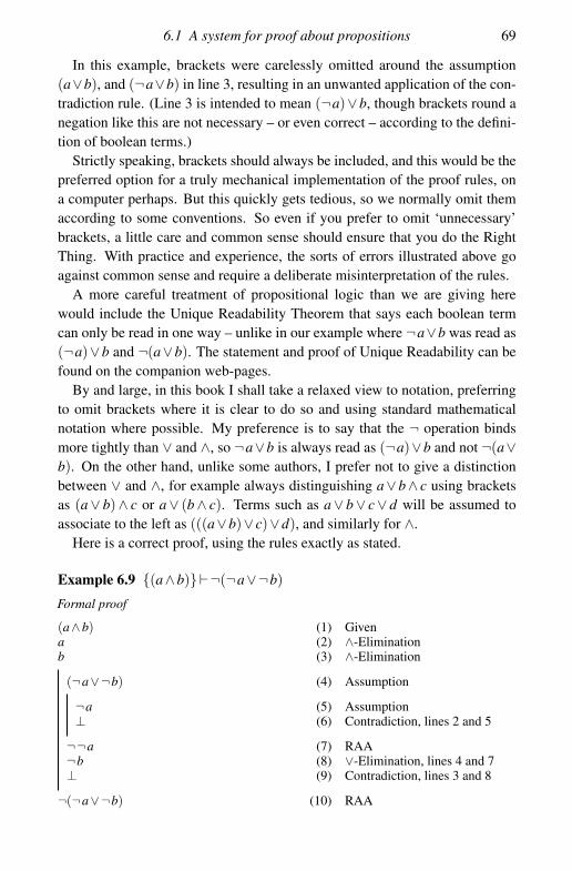
6.1 A system for proof about propositions 69
In this example, brackets were carelessly omitted around the assumption(a∨b), and (¬a∨b) in line 3, resulting in an unwanted application of the con-tradiction rule. (Line 3 is intended to mean (¬a)∨b, though brackets round anegation like this are not necessary – or even correct – according to the defini-tion of boolean terms.)
Strictly speaking, brackets should always be included, and this would be thepreferred option for a truly mechanical implementation of the proof rules, ona computer perhaps. But this quickly gets tedious, so we normally omit themaccording to some conventions. So even if you prefer to omit ‘unnecessary’brackets, a little care and common sense should ensure that you do the RightThing. With practice and experience, the sorts of errors illustrated above goagainst common sense and require a deliberate misinterpretation of the rules.
A more careful treatment of propositional logic than we are giving herewould include the Unique Readability Theorem that says each boolean termcan only be read in one way – unlike in our example where ¬a∨b was read as(¬a)∨b and ¬(a∨b). The statement and proof of Unique Readability can befound on the companion web-pages.
By and large, in this book I shall take a relaxed view to notation, preferringto omit brackets where it is clear to do so and using standard mathematicalnotation where possible. My preference is to say that the ¬ operation bindsmore tightly than ∨ and ∧, so ¬a∨b is always read as (¬a)∨b and not ¬(a∨b). On the other hand, unlike some authors, I prefer not to give a distinctionbetween ∨ and ∧, for example always distinguishing a∨ b∧ c using bracketsas (a∨ b)∧ c or a∨ (b∧ c). Terms such as a∨ b∨ c∨ d will be assumed toassociate to the left as (((a∨b)∨ c)∨d), and similarly for ∧.
Here is a correct proof, using the rules exactly as stated.
Example 6.9 {(a∧b)}�¬(¬a∨¬b)
Formal proof
(a∧b) (1) Givena (2) ∧-Eliminationb (3) ∧-Elimination
(¬a∨¬b) (4) Assumption
¬a (5) Assumption⊥ (6) Contradiction, lines 2 and 5
¬¬a (7) RAA¬b (8) ∨-Elimination, lines 4 and 7⊥ (9) Contradiction, lines 3 and 8
¬(¬a∨¬b) (10) RAA

70 Propositional logic
As with other systems in this book, the proof rules should be used in amechanical fashion without any attempt to interpret the symbols with ‘mean-ings’. Thus, for example, a and (¬a∨¬b) do not together give ¬b directly by∨-Elimination. The above example shows a way this problem can be circum-vented.
Manoeuvres such as ‘from α deduce ¬¬α’ and ‘from α and (¬α ∨¬β )deduce ¬β ’ are sufficiently common that they are worth learning as metaruleswhich can be safely used (when it is explained what you are doing) when theproof rules are used in a less rigid fashion. See Exercise 6.20 and the discussionfollowing for more information on metarules.
Another place where we relax notation is in the notation on the left handside of a turnstile symbol. Instead of using set theory notation with {. . .}, ∪,∅, etc., it is traditional to list formulas and sets of formulas, separating themwith commas, and regard the list as a single set of formulas, so the order offormulas in the list and any repetitions in it is ignored. This applies to boththe � turnstile of this chapter and the � turnstile that will be introduced in thenext. Thus, with all the conventions in place, the previous example would bewritten as a∧b�¬(¬a∨¬b). The empty set is written as an empty list, as in�(a∨¬a).
To many students, writing informal mathematical proofs accurately is a suf-ficiently daunting prospect. It might seem that writing formal proofs followingprecise rules is much worse. In fact, I believe that the opposite is the case, andthe formal rules add structure and suggest specific and useful proof strategiesthat not only make writing formal proofs easier, but can help in suggestingways to write informal arguments too.
When constructing a proof, the first step is to write down all the assumptionsor ‘known data’ at the top of a page and, leaving a large space, write the ‘goal’or statement-to-be-proved at the bottom. Then a small number of memorable‘proof strategies’ can be employed to generate most of the structure of theproof and (for propositional logic, at least) these can in fact generate the wholeproof with little or no real thinking required at all.
Many of the strategies are common sense from the rules. For example, oneis that, having got the statement α ∧β it makes sense to deduce immediatelyα and β by ∧-Elimination. This was done for example in lines 2 and 3 of theprevious example.
Another strategy is that, to prove a statement ¬α it makes sense to start anew subproof with assumption α and try and to ⊥. Our required ¬α thenfollows from Reductio Ad Absurdum. This strategy was used on line 4 of theprevious example.
A variation of this strategy is also useful, but perhaps in a slightly more

6.1 A system for proof about propositions 71
limited way: to prove a statement α it is always possible to start a new subproofwith assumption ¬α and try to prove ⊥. Our required α then follows fromReductio Ad Absurdum and ¬-Elimination. You will find plenty of occasionswhere this strategy has been used. It is often essential, and even when it is notessential it can never do any harm, though it sometimes results in longer orless elegant proofs, so should probably be left as a last resort. It is also worthmentioning that any statement at all can be derived from a contradiction, aswill be shown in Example 6.10 below.
Of course, if applying a strategy such as one of these results in a new state-ment being assumed or known ‘true’ in a part of a proof, then other strategiesshould be applied to that new statement, and so on until (hopefully) the proofis complete.
The next few examples give a short but complete list of strategies for thepropositional logic with connectives �, ⊥, ¬ , ∧ , ∨.
Example 6.10 From ⊥ or ¬� any statement can be deduced.
Formal proof
⊥ (1) Given
¬θ (2) Assumption⊥ (3) Line 1
¬¬θ (4) RAAθ (5) ¬-Elimination
It is part of the rules that statements can be copied from previously deducedones. In line 3 the statement ⊥ is available from line 1, so a contradiction isimmediate. If you prefer, think of line 3 as repetition or ‘re-deduction’ of ⊥from whatever was used to get ⊥ in line 1.
A related formal proof shows that from ¬� we quickly get ⊥. This is asfollows.
Formal proof
¬� (1) Given� (2) Top rule⊥ (3) Contradiction, lines 1 and 2
Example 6.11 To prove the statement θ from (α ∧β ) and other given state-ments Σ, deduce both of α and β first by ∧-Elimination and prove θ from Σ,α and β .

72 Propositional logic
Formal proof
(α ∧β ) (1) Givenα (2) ∧-Eliminationβ (3) ∧-Elimination. . . (4)θ (5)
Example 6.12 To prove a statement θ from ¬(α ∨β ) and other given state-ments Σ, deduce both of ¬α and ¬β first, as shown in the following argument,and then prove θ from Σ, ¬α and ¬β .
Formal proof
¬(α ∨β ) (1) Given
α (2) Assumption(α ∨β ) (3) ∨-Introduction⊥ (4) Contradiction
¬α (5) RAA
The proof that ¬(α ∨β )�¬β is similar.
It is not so easy to see how to use a statement of the form (α ∨ β ) as an‘input’, since we are not told which of α and β is true. The solution in suchcases is to construct proofs from both α and β .
Example 6.13 To prove a statement θ from (α∨β ) and other given statementsΣ, try to construct two proofs of θ , one from α and Σ, and the other from βand Σ. The final argument can be put together like this.
Formal proof
(α ∨β ) (1) Given
¬θ (2) Assumption
α (3) Assumption. . . (4)θ (5) From α, Σ�θ⊥ (6) Contradiction
¬α (7) RAAβ (8) ∨-Elimination, lines 1 and 7. . . (9)θ (10) From β , Σ�θ⊥ (11) Contradiction
¬¬θ (12) RAAθ (13) ¬-Elimination

6.1 A system for proof about propositions 73
In the special case when θ is ⊥, the previous proof simplifies to the followingformal proof.
Formal proof
(α ∨β ) (1) Given
α (2) Assumption. . . (3)⊥ (4) From α, Σ�⊥
¬α (5) RAAβ (6) ∨-Elimination, lines 1 and 7. . . (7)⊥ (8) From β , Σ�⊥
Using a given statement of the form ¬(α ∧ β ) is similar to the case usinga statement (¬α ∨¬β ), and you should construct two proofs and put themtogether using an assumption and subproof.
Example 6.14 To prove a statement θ from ¬(α ∧β ) and other statements Σ,construct two proofs of θ , one from ¬α and Σ, and the other from ¬β and Σ.
Formal proof
¬(α ∧β ) (1) Given
¬θ (2) Assumption
¬α (3) Assumption. . . (4)θ (5) From ¬α, Σ�θ⊥ (6) Contradiction
¬¬α (7) RAAα (8) ¬-Elimination
¬β (9) Assumption. . . (10)θ (11) From ¬β , Σ�θ⊥ (12) Contradiction
¬¬β (13) RAAβ (14) ¬-Elimination(α ∧β ) (15) ∧-Introduction⊥ (16) Contradiction, lines 1 and 15
¬¬θ (17) RAAθ (18) ¬-Elimination
In the special case when θ is ⊥, this simplifies to the following formal proof.
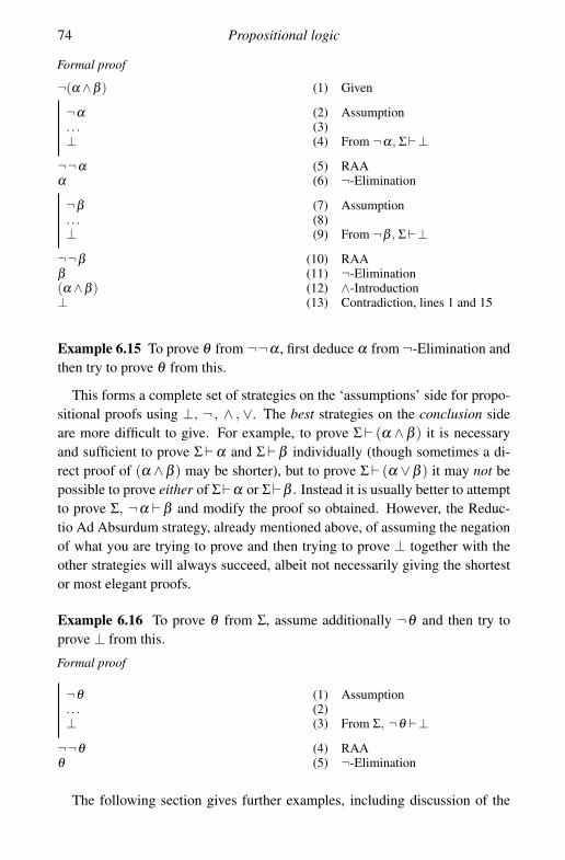
74 Propositional logic
Formal proof
¬(α ∧β ) (1) Given
¬α (2) Assumption. . . (3)⊥ (4) From ¬α, Σ�⊥
¬¬α (5) RAAα (6) ¬-Elimination
¬β (7) Assumption. . . (8)⊥ (9) From ¬β , Σ�⊥
¬¬β (10) RAAβ (11) ¬-Elimination(α ∧β ) (12) ∧-Introduction⊥ (13) Contradiction, lines 1 and 15
Example 6.15 To prove θ from ¬¬α , first deduce α from ¬-Elimination andthen try to prove θ from this.
This forms a complete set of strategies on the ‘assumptions’ side for propo-sitional proofs using ⊥, ¬ , ∧ , ∨. The best strategies on the conclusion sideare more difficult to give. For example, to prove Σ� (α ∧ β ) it is necessaryand sufficient to prove Σ�α and Σ�β individually (though sometimes a di-rect proof of (α ∧β ) may be shorter), but to prove Σ� (α ∨β ) it may not bepossible to prove either of Σ�α or Σ�β . Instead it is usually better to attemptto prove Σ, ¬α �β and modify the proof so obtained. However, the Reduc-tio Ad Absurdum strategy, already mentioned above, of assuming the negationof what you are trying to prove and then trying to prove ⊥ together with theother strategies will always succeed, albeit not necessarily giving the shortestor most elegant proofs.
Example 6.16 To prove θ from Σ, assume additionally ¬θ and then try toprove ⊥ from this.
Formal proof
¬θ (1) Assumption. . . (2)⊥ (3) From Σ, ¬θ �⊥
¬¬θ (4) RAAθ (5) ¬-Elimination
The following section gives further examples, including discussion of the

6.2 Examples and exercises 75
implication operator, and the final optional section of this chapter sketchesa proof that the above examples do indeed form a complete set of strategiesthat are guaranteed to produce a proof of an assertion in propositional logic –provided, of course, that such a proof exists at all.
6.2 Examples and exercises
Exercise 6.17 Give a formal proof of the law of excluded middle which saysthat if φ is any statement or boolean term then (φ ∨¬φ) has a formal proof inthe system above.
Exercise 6.18 Find a formal proof of (¬a∨¬b) from ¬(a∧ b), and anotherformal proof for the converse.
Exercise 6.19 Give formal derivations showing the following:
• ¬ p∨q�¬¬q∨¬ p• �¬(¬ p∨⊥)∨¬ p• ¬ p∨q, ¬ p∨ r�¬ p∨ (q∧ r)• �¬ p∨ (p∨q)• ¬ p∨q�¬(¬q∨ r)∨ (¬ p∨ r)
Exercise 6.20 Show that the following rule could be added to the system with-out changing the set of statements that are provable: ‘If τ has been deducedfrom Σ∪ {¬σ}, then (σ ∨ τ) may be deduced from Σ in one further step.’(Hint: show how to transform a proof of τ from Σ∪{¬σ} to one of (σ ∨ τ)from Σ.)
The last exercise shows how ‘metarules’ can be added to the system; suchrules can simplify the process of finding formal proofs considerably, as well asshortening and making the resulting proofs more readable.
As an example of metarules, note that the ∨-elimination rule is quite trickyas it is only available in one limited form, and like all the other rules it is asyntactic rule and only applies when the symbols combine in exactly the waystated in the rule. Fortunately, all the other forms that most people expect to bepresent can be justified as metarules.
Exercise 6.21 Show that addition of the following metarules to the systemdoes not change the set of sentences provable.
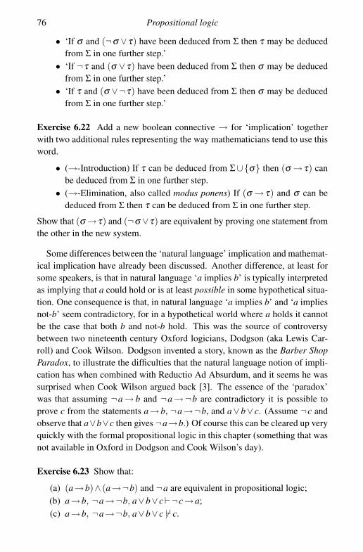
76 Propositional logic
• ‘If σ and (¬σ ∨ τ) have been deduced from Σ then τ may be deducedfrom Σ in one further step.’
• ‘If ¬τ and (σ ∨ τ) have been deduced from Σ then σ may be deducedfrom Σ in one further step.’
• ‘If τ and (σ ∨¬τ) have been deduced from Σ then σ may be deducedfrom Σ in one further step.’
Exercise 6.22 Add a new boolean connective → for ‘implication’ togetherwith two additional rules representing the way mathematicians tend to use thisword.
• (→-Introduction) If τ can be deduced from Σ∪{σ} then (σ → τ) canbe deduced from Σ in one further step.
• (→-Elimination, also called modus ponens) If (σ → τ) and σ can bededuced from Σ then τ can be deduced from Σ in one further step.
Show that (σ →τ) and (¬σ ∨τ) are equivalent by proving one statement fromthe other in the new system.
Some differences between the ‘natural language’ implication and mathemat-ical implication have already been discussed. Another difference, at least forsome speakers, is that in natural language ‘a implies b’ is typically interpretedas implying that a could hold or is at least possible in some hypothetical situa-tion. One consequence is that, in natural language ‘a implies b’ and ‘a impliesnot-b’ seem contradictory, for in a hypothetical world where a holds it cannotbe the case that both b and not-b hold. This was the source of controversybetween two nineteenth century Oxford logicians, Dodgson (aka Lewis Car-roll) and Cook Wilson. Dodgson invented a story, known as the Barber ShopParadox, to illustrate the difficulties that the natural language notion of impli-cation has when combined with Reductio Ad Absurdum, and it seems he wassurprised when Cook Wilson argued back [3]. The essence of the ‘paradox’was that assuming ¬a→ b and ¬a→¬b are contradictory it is possible toprove c from the statements a→b, ¬a→¬b, and a∨b∨ c. (Assume ¬c andobserve that a∨b∨c then gives ¬a→b.) Of course this can be cleared up veryquickly with the formal propositional logic in this chapter (something that wasnot available in Oxford in Dodgson and Cook Wilson’s day).
Exercise 6.23 Show that:
(a) (a→b)∧ (a→¬b) and ¬a are equivalent in propositional logic;(b) a→b, ¬a→¬b, a∨b∨ c�¬c→a;(c) a→b, ¬a→¬b, a∨b∨ c � � c.

6.3 Decidability of propositional logic* 77
(Part (c) is possibly too hard at this stage, but will become easy with the resultsof the next chapter.)
We have seen many kinds of implication in this book, including the informaluse of ‘implies’ in our metatheorems and metaproofs, �, �, and now →. Theyare all different (albeit, related) and it is important to be able to distinguishbetween them all. The next exercises point out some connections between �and →.
Exercise 6.24 Prove the Deduction Theorem that says that Σ∪{σ}� τ is trueif and only if Σ�σ →τ is true, where � is for the extended system with the ad-ditional rules for → added. (The Deduction Theorem is quite straightforwardfor the system we have here given the rules for →, but for other formal systemsbecomes an important result.)
Exercise 6.25 Show that (a) ¬θ �¬ψ implies ψ �θ , and (b) in the proposi-tional logic with → added we have
�((¬θ →¬ψ)→ (ψ →θ)).
In what ways are statements (a) and (b) different?
6.3 Decidability of propositional logic*
Given a finite set of boolean terms Σ and a further boolean term σ we mayask whether Σ� σ . More generally, the data Σ, σ being finite could be theinput to a computer program, and we could ask whether there is an algorithm,programmable on a computer, that correctly tells us whether Σ � σ , and, ifpossible, generates a formal proof too.
For propositional logic, this is indeed possible. One method uses valuations,as discussed in the next chapter, but this method simply yields a yes/no answer,not a formal proof. Another method uses the proof strategies discussed infor-mally in the text above.
The idea of the algorithm is to reduce the question ‘does Σ�σ?’ to ‘simpler’questions, and working backwards each stage of the reduction gives a recipeof how to transform proofs of the ‘simpler’ questions to one of the original.More precisely, the following theorem (which is a formal statement of the ideaof proof strategies discussed above) allows us to reduce Σ� σ to a numberof questions about provability of statements with no ∧, ∨, or double negationsymbols.

78 Propositional logic
Theorem 6.26 Let X be a set of propositional letters, Σ a finite set of booleanterms in X, and α, β , σ other boolean terms in X. Then:
(i) Σ�σ if and only if Σ, ¬σ �⊥;(ii) Σ, ¬¬α �⊥ if and only if Σ, α �⊥;
(iii) Σ, α ∧β �⊥ if and only if Σ, α, β �⊥;(iv) Σ, ¬(α ∨β )�⊥ if and only if Σ, ¬α, ¬β �⊥;(v) Σ, α ∨β �⊥ if and only if Σ, α �⊥ and Σ, β �⊥;
(vi) Σ, ¬(α ∧β )�⊥ if and only if Σ, ¬α �⊥ and Σ, ¬β �⊥.
Proof The right-to-left directions were covered in examples earlier in thischapter. The other directions are done in a similar way.
(i) If Σ�σ then Σ, ¬σ �⊥ as
Formal proof
¬σ (1) Given. . . (2)σ (3) From Σ�σ⊥ (4) Contradiction, lines 1 and 3
(ii) If Σ, ¬¬α �⊥ then Σ, α �⊥ as
Formal proof
α (1) Given
¬α (2) Assumption⊥ (3) Contradiction, lines 1 and 2
¬¬α (4) RAA. . . (5)⊥ (6) From Σ, ¬¬α �⊥
The other cases are similarly easy, and we leave them as exercises.
By iterating the previous theorem, we see that any statement of the form Σ�σis equivalent to a number of statements of the form Π�⊥, where each α ∈ Πis either �, ⊥, ¬�, ¬⊥, or a or ¬a for some propositional letter a. What ismore, the proof of the theorem shows how we can transform formal proofs ofall the statements Π�⊥ back into a proof of the original Σ�σ .
Statements of the form �, ⊥, or a are called atomic. Those of the form¬�, ¬⊥, or ¬a are called negated atomic. This means that we can reduceour problem of whether Σ�σ to the case where σ = ⊥ and Σ consists of onlyatomic or negated atomic statements. Now two cases when such a set Σ isobviously contradictory are (a) when Σ contains ⊥ or ¬�, and (b) when Σ

6.3 Decidability of propositional logic* 79
contains both a and ¬a for some letter a. In fact, this is the only way such aset Σ can prove ⊥, as the following shows.
Theorem 6.27 Let Σ consist of atomic and negated atomic statements only.Then Σ�⊥ if and only if Σ contains ⊥ or ¬�, or both a and ¬a for someletter a.
I am not going to prove this here. The difficult direction is to show that ifΣ does not contain ⊥ nor ¬�, nor both a and ¬a for some a, then Σ � �⊥, andthe worry is that somehow the rules for ∨ or ∧ might be used in a way that wehave not yet envisaged. One method (that will be discussed in more detail inthe next chapter) is to define a semantics making every statement a occurringin Σ ‘true’ and every other letter b ‘false’ and use this as a basis for inductionon the length of proofs. Another method, also by induction on the length ofproofs, is to show that if such Σ�⊥ then there is a proof that does not use anyof the rules for ∨ or ∧.
Either way, our discussion yields the following theorem.
Theorem 6.28 There is an algorithm which, on input Σ and σ (a finite setof statements and a single statement in the propositional logic) correctly de-termines whether Σ�σ , and in case the answer is ‘yes’ also returns a formalproof of σ from Σ.

7
Valuations
7.1 Semantics for propositional logic
Following the general method for other formal systems in this book, we mustconnect the system for propositional logic of the last chapter with the booleanalgebras of the chapter preceding it, by using boolean algebras to provide‘meanings’ or semantics for boolean terms and the symbolic manipulationsin the system for proof. As for other logics in this book, we will develop oursemantics far enough to present a Completeness Theorem and a SoundnessTheorem. The basis of our semantics is the following very simple idea of avaluation.
Definition 7.1 Let X be any set, and B a boolean algebra. A valuation on X isa function f : X →B.
This notion of a valuation is very straightforward, but is enough to givea valuation v: X →B interesting extra structure. A valuation induces a mapBT(X)→B defined by evaluating boolean terms over X in the boolean algebraB, using the value v(x) in place of the symbol x from X and the operations inB for all other terms. Formally, this means making the following definition byinduction on the number of symbols in a term:
• v(¬σ) = (v(σ))′
• v(σ ∧ τ) = (v(σ))∧ (v(τ))• v(σ ∨ τ) = (v(σ))∨ (v(τ))• v(�) = �• v(⊥) = ⊥
where the right hand side of each of these is evaluated in B using its booleanalgebra structure. Remember that the arguments inside the v(. . .) are simplyformal terms, i.e. strings of symbols in the appropriate alphabet, so the symbols
80
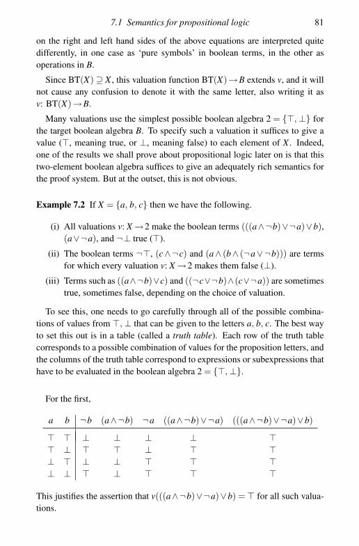
7.1 Semantics for propositional logic 81
on the right and left hand sides of the above equations are interpreted quitedifferently, in one case as ‘pure symbols’ in boolean terms, in the other asoperations in B.
Since BT(X) ⊇ X , this valuation function BT(X)→B extends v, and it willnot cause any confusion to denote it with the same letter, also writing it asv: BT(X)→B.
Many valuations use the simplest possible boolean algebra 2 = {�, ⊥} forthe target boolean algebra B. To specify such a valuation it suffices to give avalue (�, meaning true, or ⊥, meaning false) to each element of X . Indeed,one of the results we shall prove about propositional logic later on is that thistwo-element boolean algebra suffices to give an adequately rich semantics forthe proof system. But at the outset, this is not obvious.
Example 7.2 If X = {a, b, c} then we have the following.
(i) All valuations v: X →2 make the boolean terms (((a∧¬b)∨¬a)∨b),(a∨¬a), and ¬⊥ true (�).
(ii) The boolean terms ¬�, (c∧¬c) and (a∧ (b∧ (¬a∨¬b))) are termsfor which every valuation v: X →2 makes them false (⊥).
(iii) Terms such as ((a∧¬b)∨c) and ((¬c∨¬b)∧(c∨¬a)) are sometimestrue, sometimes false, depending on the choice of valuation.
To see this, one needs to go carefully through all of the possible combina-tions of values from �, ⊥ that can be given to the letters a, b, c. The best wayto set this out is in a table (called a truth table). Each row of the truth tablecorresponds to a possible combination of values for the proposition letters, andthe columns of the truth table correspond to expressions or subexpressions thathave to be evaluated in the boolean algebra 2 = {�, ⊥}.
For the first,
a b ¬b (a∧¬b) ¬a ((a∧¬b)∨¬a) (((a∧¬b)∨¬a)∨b)
� � ⊥ ⊥ ⊥ ⊥ �� ⊥ � � ⊥ � �⊥ � ⊥ ⊥ � � �⊥ ⊥ � ⊥ � � �
This justifies the assertion that v(((a∧¬b)∨¬a)∨b) = � for all such valua-tions.
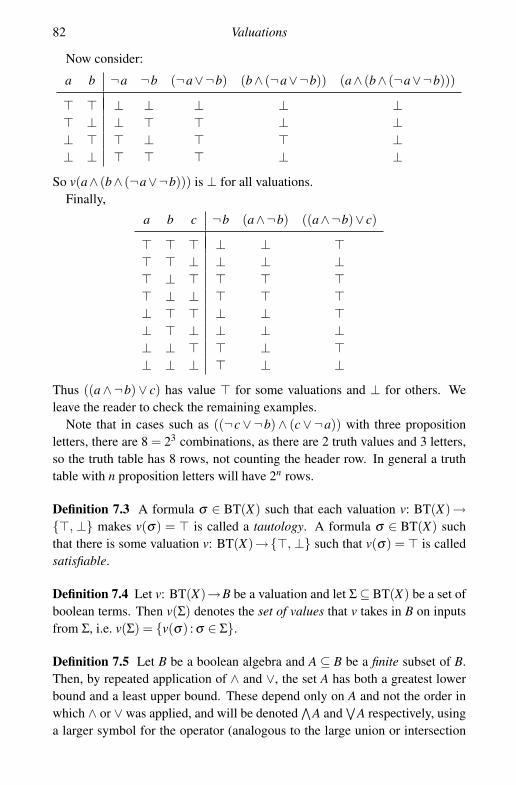
82 Valuations
Now consider:
a b ¬a ¬b (¬a∨¬b) (b∧ (¬a∨¬b)) (a∧ (b∧ (¬a∨¬b)))
� � ⊥ ⊥ ⊥ ⊥ ⊥� ⊥ ⊥ � � ⊥ ⊥⊥ � � ⊥ � � ⊥⊥ ⊥ � � � ⊥ ⊥
So v(a∧ (b∧ (¬a∨¬b))) is ⊥ for all valuations.Finally,
a b c ¬b (a∧¬b) ((a∧¬b)∨ c)
� � � ⊥ ⊥ �� � ⊥ ⊥ ⊥ ⊥� ⊥ � � � �� ⊥ ⊥ � � �⊥ � � ⊥ ⊥ �⊥ � ⊥ ⊥ ⊥ ⊥⊥ ⊥ � � ⊥ �⊥ ⊥ ⊥ � ⊥ ⊥
Thus ((a∧¬b)∨ c) has value � for some valuations and ⊥ for others. Weleave the reader to check the remaining examples.
Note that in cases such as ((¬c∨¬b)∧ (c∨¬a)) with three propositionletters, there are 8 = 23 combinations, as there are 2 truth values and 3 letters,so the truth table has 8 rows, not counting the header row. In general a truthtable with n proposition letters will have 2n rows.
Definition 7.3 A formula σ ∈ BT(X) such that each valuation v: BT(X)→{�, ⊥} makes v(σ) = � is called a tautology. A formula σ ∈ BT(X) suchthat there is some valuation v: BT(X)→{�, ⊥} such that v(σ) = � is calledsatisfiable.
Definition 7.4 Let v: BT(X)→B be a valuation and let Σ ⊆ BT(X) be a set ofboolean terms. Then v(Σ) denotes the set of values that v takes in B on inputsfrom Σ, i.e. v(Σ) = {v(σ) : σ ∈ Σ}.
Definition 7.5 Let B be a boolean algebra and A ⊆ B be a finite subset of B.Then, by repeated application of ∧ and ∨, the set A has both a greatest lowerbound and a least upper bound. These depend only on A and not the order inwhich ∧ or ∨ was applied, and will be denoted
∧A and
∨A respectively, using
a larger symbol for the operator (analogous to the large union or intersection

7.1 Semantics for propositional logic 83
signs⋃
,⋂
or the large summation and product signs ∑ , ∏). To cover the casewhen A is empty, we conventionally define
∧∅ = � and
∨∅ = ⊥.
There are boolean algebras in which∧
A and∨
A are defined for all sets A,not just the finite ones. The power set algebra P(X) of a set X is an example.These are interesting algebras, but not every one is of this type. To ensure thatour results apply to all boolean algebras, we will take care to apply
∧and
∨to
finite sets only.Here is the formal definition of semantics, �. It says that Σ�σ holds if σ is
at least as true as the greatest lower bound (or ‘and’) of some finite subset of Σ.(We cannot take the whole of Σ, in case that Σ itself is infinite.) To measure ‘atleast as true’ we use boolean algebras and valuations.
Definition 7.6 Given a set X , Σ ⊆ BT(X) and σ ∈ BT(X) we write Σ � σ forthe statement that, for all boolean algebras B and all valuations v: BT(X)→B,there is a finite subset Σ0 ⊆ Σ such that
∧v(Σ0) � v(σ).
Definition 7.7 We write Σ �2 σ for the specialisation of Σ � σ to the booleanalgebra 2 = {�, ⊥}. That is, Σ �2 σ means for all valuations v: BT(X)→ 2,there is a finite subset Σ0 ⊆ Σ such that
∧v(Σ0) � v(σ).
Once again, truth tables can help calculate whether Σ�2 σ holds or not.
Example 7.8 Given proposition letters p, q we have
p, ¬(p∧ r)�2 ¬((p∨q)∧ r).
The truth table is
p q r p ¬(p∧ r) ¬((p∨q)∧ r)
� � � � ⊥ ⊥� � ⊥ � � �� ⊥ � � ⊥ ⊥� ⊥ ⊥ � � �⊥ � � ⊥ � ⊥⊥ � ⊥ ⊥ � �⊥ ⊥ � ⊥ � �⊥ ⊥ ⊥ ⊥ � �
Observe that in each of the two rows in which both p and ¬(p∧ r) are � (thesecond and fourth), the conclusion ¬((p∨q)∧ r) is also �. This suffices. Thefact that the conclusion is also true in additional rows is irrelevant.

84 Valuations
Example 7.9 Again, with proposition letters p, q we have
¬(q∧ r), (p∨ r) ��2 p∧ (¬q∨ r).
The truth table is
p q r ¬(q∧ r) (p∨ r) p∧ (¬q∨ r)
� � � ⊥ � �� � ⊥ � � ⊥� ⊥ � � � �� ⊥ ⊥ � � �⊥ � � ⊥ � ⊥⊥ � ⊥ � ⊥ ⊥⊥ ⊥ � � � ⊥⊥ ⊥ ⊥ � ⊥ ⊥
Here, we see that the valuation v(p) = ⊥, v(q) = ⊥, v(r) = � makes ¬(q∧ r)and p∨ r both equal to � but makes the conclusion p∧ (¬q∨ r) equal to ⊥, so¬(q∧ r), (p∨ r)�2 p∧ (¬q∨ r) is false.
Theorem 7.10 (Soundness Theorem) Let X be a set and τ ∈ BT(X), andsuppose that Σ� τ . Then Σ� τ .
Proof Let B be a boolean algebra and v: BT(X)→B a valuation. Let Σ0 be theset of assumptions used in Σ to prove τ . We shall prove
∧v(Σ0) � v(τ). To
simplify notation we will assume without loss of generality that Σ is finite andΣ0 = Σ.
So we must prove that if there is a formal derivation of τ from Σ then thevalue of the conclusion of such a formal derivation, v(τ), is always ‘at least astrue as’ the value of the assumptions, Σ. In particular if v(σ) =� for all σ ∈ Σthen � =
∧v(Σ) � v(τ), so v(τ) = �.
The proof is by induction on the length of a derivation. Our induction hy-pothesis H(n) is the statement that if p is a derivation in the system with atmost n steps and p is a proof of τ from a finite set of assumptions Σ, then∧
v(Σ) � v(τ) for all valuations v on BT(X).Assume we have such a derivation p of length n of τ from a finite set Σ, that
H(n− 1) holds, and that v is a valuation. As before, we look at the very lastdeduction in p.
The cases when the last deduction used is either the Top Rule or the GivenStatements Rule is easy, since in the first of these cases τ is � and v(�) =��∧
v(Σ), and in the second of these cases τ is some σ ∈Σ and hence v(τ) = v(σ)for some σ ∈ Σ so v(τ) � ∧
v(Σ).

7.1 Semantics for propositional logic 85
If the last step in p is ∧-Introduction then τ is (α ∧ β ) where α, β havepreviously been derived from Σ. Thus v(α), v(β ) � ∧
v(Σ) by the inductionhypothesis and so
∧v(Σ) is a lower bound for both v(α), v(β ), hence v(α ∧
β ) = v(α)∧ v(β ) � ∧v(Σ).
If the last step in p is ∧-Elimination then τ is α or β where (α ∧β ) has beenpreviously derived from Σ. So by the induction hypothesis v(α ∧β ) � ∧
v(Σ).And as v(α ∧β ) = v(α)∧v(β ) � v(α), v(β ) we have v(α), v(β ) � ∧
v(Σ) bytransitivity.
If the last step in p is ∨-Elimination then (σ ∨ τ) and ¬σ have alreadybeen deduced from Σ so by the induction hypothesis v(σ ∨τ) = v(σ)∨v(τ) �∧
v(Σ) and v(¬σ) = v(σ)′ � ∧v(Σ). So from v(σ)∨ v(τ) � ∧
v(Σ) we have
v(σ)′ ∧ (v(σ)∨ v(τ)) � v(σ)′ ∧∧
v(Σ).
And from v(σ)′ � ∧v(Σ) we have
v(σ)′ ∧∧
v(Σ) =∧
v(Σ).
Also
v(σ)′ ∧ (v(σ)∨ v(τ)) = v(σ ′)∧ v(τ)
by distributivity, so v(τ) � v(σ ′)∧ v(τ) � ∧v(Σ), as required.
If the last step in p is ¬-Elimination then ¬¬τ has already been derived sov(¬¬τ) = v(τ)′′ = v(τ) � ∧
v(Σ), as required.If the last step is the Contradiction Rule, both σ and ¬σ have already been
derived with v(σ), v(¬σ) � ∧v(Σ). So
∧v(Σ) is a lower bound for v(σ) and
v(¬σ) = v(σ)′ so ⊥ = v(σ)∧ v(σ)′ � ∧v(Σ), as required.
If the last step is the ∨-Introduction Rule, assume that τ is (α∨β ) or (β ∨α)where α has been deduced from Σ. Then by our induction hypothesis v(α) �∧
v(Σ), so
v(α ∨β ), v(β ∨α) � v(α) �∧
v(Σ)
as required.Finally, the Reductio Ad Absurdum Rule: if ⊥ has been deduced from Σ∪
{α} then by the induction hypothesis ⊥ = v(⊥) � ∧v(Σ)∧ v(α) so v(¬α) =
v(α)′ ∨ v(⊥) � v(α)′ ∨ (∧
v(Σ)∧ v(α)). But
v(α)′ ∨ (∧
v(Σ)∧ v(α)) = v(α)′ ∨∧
v(Σ) �∧
v(Σ)
by distributivity, so v(¬α) = v(α)′ � ∧v(Σ) as required.
The Completeness Theorem for propositional logic takes the form ‘Σ � φ im-plies Σ� φ ’ and says that any statement φ that follows from Σ in the sense

86 Valuations
of boolean algebras, i.e. any φ whose valuation is at least as true as that ofΣ however these valuations are chosen, actually has a formal derivation fromassumptions Σ in the formal system. This is hardly an obvious assertion sincethe rules for the formal system are limited and coming up with formal proofscan be rather difficult, even for specific cases, let alone in general. It turns outthat the Completeness Theorem is a strong and useful result for mathematics.In the next chapter we shall also look at what it has to say for boolean algebrasin particular.
From a more philosophical point of view, the Completeness Theorem showsthat any correct deduction about propositions or boolean terms can alwaysbe rewritten as a formal deduction in a specific formal system. By a ‘correctdeduction’ here, we mean one that is ‘semantically correct’, i.e. one that can beshown to be correct in all possible cases by considering valuations into booleanalgebras. There is a considerable saving here as the Completeness Theoremshows that any deduction given by any correct method can be replaced byone of a specific form using one particular proof system. In other words, theformal system is complete in the sense that it can make all necessary logicaldeductions about the statements that can be expressed in it. As a bonus, therules of our formal system were chosen specifically to mimic real mathematicalpractice and we know them to be correct, because of the Soundness Theorem.Furthermore, these rules can be checked mechanically too.
We are now going to prove the Completeness Theorem. First, we need alemma. Recall that a set Σ ⊆ BT(X) is consistent if Σ � �⊥.
Lemma 7.11 Suppose X is a set of propositional letters, Σ ⊆ BT(X) is con-sistent, and φ ∈ BT(X). Then either Σ∪ {φ} is consistent or Σ∪ {¬φ} isconsistent.
Proof If Σ∪{φ}�⊥ and Σ∪{¬φ}�⊥ then by the first of these and ReductioAd Absurdum Σ�¬φ . By appending a proof of ⊥ from Σ∪{¬φ} (given bythe second of our assumptions) on to the end of a proof for Σ�¬φ we obtaina proof of ⊥ from Σ, hence Σ is inconsistent.
Theorem 7.12 (Completeness Theorem, first form) Let X be a set, andsuppose that Σ0 ⊆ BT(X) is consistent. Then there is a valuation v: BT(X)→{�, ⊥} such that v(σ) = � for all σ ∈ Σ0.
Proof Somehow we have to define an appropriate valuation, and this mayinvolve making choices for the value of the letters in X . This already suggeststhat if X is not finite then we will need to use Zorn’s Lemma.

7.1 Semantics for propositional logic 87
It is not obvious how to use Zorn’s Lemma directly, as decisions on thevalue v(x) to give to a propositional letter x ∈ X can have rather subtle conse-quences. So instead we use our system of formal derivations to ‘control’ whatis going on.
We consider the set Z = {Σ ⊆ BT(X) : Σ ⊇ Σ0 and Σ � �⊥} of all consistentextensions of Σ0. This is a poset, where the order relation is ⊆. We claim thatZ has the Zorn property and so has a maximal element.
To see this, let C ⊆ Z be a chain. So each element of C is a set Σ such thatΣ ⊇ Σ0 and Σ � �⊥. Now consider ΣC =
⋃C. Clearly ΣC is an upper bound for
C, we just need to show that it is in Z. First, ΣC extends Σ0 as each element ofC does. Now suppose ΣC�⊥. Then there is a single derivation p from ΣC of ⊥.This derivation is finite so only requires finitely many assumptions from ΣC.Each of these assumptions comes from some Σ ∈ C, and as there are finitelymany assumptions, only finitely many Σ ∈C are required, and of these there isa ⊆-largest one, Π say, since C is a chain. Therefore the derivation p can beregarded as a derivation Π�⊥, but this is impossible as Π ∈ Z so by definitionis consistent. Hence ΣC is consistent.
By the previous paragraph and Zorn’s Lemma there is a maximal elementΣmax in Z. Note that by Lemma 7.11 this has the property that for any φ ∈BT(X) either φ ∈ Σmax or ¬φ ∈ Σmax, for otherwise from the lemma we coulddeduce that one of Σmax∪{φ} or Σmax∪{¬φ} is a proper consistent extensionof Σmax, contradicting maximality. Furthermore we cannot have both of φ , ¬φin Σmax since that would mean that Σmax would be inconsistent by the Contra-diction Rule. Note also that by the same argument � ∈ Σmax and ¬⊥ ∈ Σmax
since both {¬�} and {⊥} are inconsistent.We may now define our valuation by v(x) = � if x ∈ Σmax and v(x) = ⊥ if
¬x ∈ Σmax. By the previous paragraph this does indeed define a valuation andwe just need to show that v(σ) = � for each σ ∈ Σ0. We shall in fact showv(σ) = � for each σ ∈ Σmax, which suffices as Σ0 ⊆ Σmax.
The proof that v(σ) = � for each σ ∈ Σmax is by induction on the numberof symbols in σ ∈ BT(X). Our induction hypothesis H(n) is the statement thatif σ contains at most n symbols then
v(σ) = � if and only if σ ∈ Σmax.
This statement is true for n = 1 since the only elements of σ ∈ BT(X) with onesymbol are �, ⊥ or elements of X and these have been dealt with already bythe definition of v.
If σ has n+1 symbols and is ¬τ for some τ then we have by the inductionhypothesis v(τ) =� if and only if τ ∈ Σmax. If ¬τ ∈ Σmax then τ �∈ Σmax sinceotherwise Σmax would be inconsistent and v(τ) =⊥ so v(¬τ) = v(τ)′ =�. On
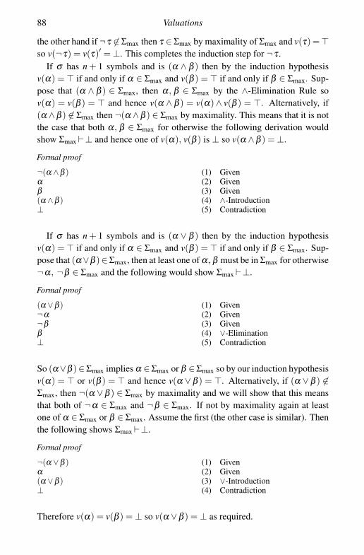
88 Valuations
the other hand if ¬τ �∈ Σmax then τ ∈ Σmax by maximality of Σmax and v(τ) =�so v(¬τ) = v(τ)′ = ⊥. This completes the induction step for ¬τ .
If σ has n + 1 symbols and is (α ∧ β ) then by the induction hypothesisv(α) = � if and only if α ∈ Σmax and v(β ) = � if and only if β ∈ Σmax. Sup-pose that (α ∧ β ) ∈ Σmax, then α, β ∈ Σmax by the ∧-Elimination Rule sov(α) = v(β ) = � and hence v(α ∧ β ) = v(α)∧ v(β ) = �. Alternatively, if(α ∧β ) �∈ Σmax then ¬(α ∧β ) ∈ Σmax by maximality. This means that it is notthe case that both α, β ∈ Σmax for otherwise the following derivation wouldshow Σmax �⊥ and hence one of v(α), v(β ) is ⊥ so v(α ∧β ) = ⊥.
Formal proof
¬(α ∧β ) (1) Givenα (2) Givenβ (3) Given(α ∧β ) (4) ∧-Introduction⊥ (5) Contradiction
If σ has n + 1 symbols and is (α ∨ β ) then by the induction hypothesisv(α) = � if and only if α ∈ Σmax and v(β ) = � if and only if β ∈ Σmax. Sup-pose that (α∨β )∈Σmax, then at least one of α , β must be in Σmax for otherwise¬α, ¬β ∈ Σmax and the following would show Σmax �⊥.
Formal proof
(α ∨β ) (1) Given¬α (2) Given¬β (3) Givenβ (4) ∨-Elimination⊥ (5) Contradiction
So (α∨β )∈Σmax implies α ∈Σmax or β ∈Σmax so by our induction hypothesisv(α) = � or v(β ) = � and hence v(α ∨β ) = �. Alternatively, if (α ∨β ) �∈Σmax, then ¬(α ∨β ) ∈ Σmax by maximality and we will show that this meansthat both of ¬α ∈ Σmax and ¬β ∈ Σmax. If not by maximality again at leastone of α ∈ Σmax or β ∈ Σmax. Assume the first (the other case is similar). Thenthe following shows Σmax �⊥.
Formal proof
¬(α ∨β ) (1) Givenα (2) Given(α ∨β ) (3) ∨-Introduction⊥ (4) Contradiction
Therefore v(α) = v(β ) = ⊥ so v(α ∨β ) = ⊥ as required.

7.1 Semantics for propositional logic 89
This completes the induction proof and therefore v is a valuation making allof Σmax (and hence Σ0) true, as required.
Theorem 7.13 (Completeness Theorem, second form) Let X be a set, andsuppose that Σ ⊆ BT(X) and τ ∈ BT(X) with Σ� τ , or just Σ�2 τ . Then Σ� τ ,i.e. there is a formal derivation of τ from Σ.
Proof Assume Σ � �τ . Then Σ∪{¬τ} ��⊥ since if otherwise we would have Σ�¬¬τ by Reductio Ad Absurdum and hence Σ� τ by ¬-Elimination. But thenthe first form of the Completeness Theorem gives us a valuation v: BT(X)→{�, ⊥} with v(σ) = � for all σ ∈ Σ and v(¬τ) = v(τ)′ = � hence v(τ) = ⊥.So
∧v(Σ) = � > v(τ) and hence Σ �� τ .
Many of the more interesting consequences of completeness and soundness areconnected with the finite nature of proofs. We can express this connection inthe following important result.
Theorem 7.14 (Compactness Theorem) Let X be an infinite set and letΣ ⊆ BT(X). Suppose that for every finite subset Σ0 ⊆ Σ there is a valuationv0: BT(X)→{�, ⊥} such that v0(σ) =� for all σ ∈Σ0. Then there is a singlevaluation v: BT(X)→{�, ⊥} such that v(σ) = � for all σ ∈ Σ.
Proof By hypothesis, and the Soundness Theorem, every finite subset of Σis consistent. It follows that the whole of Σ is consistent since if Σ�⊥ thenthere is a finite proof of ⊥ from Σ, which necessarily uses only finitely manyassumptions from Σ. This would imply that some finite subset of Σ is incon-sistent, contrary to hypothesis. So Σ � � ⊥ and by the Completeness Theoremthere is a valuation as indicated.
Finally, to sum up this section, we have looked at boolean algebras in general,and the boolean algebra 2 = {�, ⊥} in particular, and proved a version of theSoundness Theorem for general boolean algebras and a version of the Com-pleteness Theorem for the particular boolean algebra {�, ⊥}. The results weproved show that, for any set of boolean terms Σ and any other statement σ
Σ�2 σ implies Σ�σ
(the Completeness Theorem), and
Σ�σ implies Σ�σ
(the Soundness Theorem). It is a triviality from the definition that
Σ�σ implies Σ�2 σ

90 Valuations
since 2 = {�, ⊥} is an example boolean algebra that can be used in the defini-tion of Σ�σ . Thus we have proved the following.
Corollary 7.15 For any set of boolean terms Σ and any other statement σ ,
Σ�σ if and only if Σ�2 σ .
This is hardly obvious, but the equivalence of all these statements is of greatinterest as it allows us to decide statements of the form Σ�σ by looking atvaluations to the boolean algebra 2, and this is a great help as this algebra isparticularly easy to compute in. In particular, from Example 7.8 we can nowdeduce that p, ¬(p∧r)�(p∨q)∧r without having to construct a formal proofdirectly, and from Example 7.9 we can see that ¬(q∧r), (p∨r) � � p∧(¬q∨r).This last fact would have been difficult to deduce directly from the formalsystem alone without the help of the Soundness Theorem.
7.2 Examples and exercises
We have used boolean algebras to represent the more traditional material on‘propositional logic’. The Soundness and the Completeness Theorems give aconnection between the two sides of the story: semantics or meanings, givenby boolean algebras in general or by the particular boolean algebra 2 = {�, ⊥}on the one hand, and the propositions or boolean terms themselves consideredas strings of symbols, and formal proofs involving them on the other hand.The side involving boolean terms and formal proofs is useful since a proofis mechanically checkable and therefore incontrovertibly a proof of what itclaims to be. The semantics side is often easier to use when it comes to provingthat something is not derivable.
Exercise 7.16 Show that the following hold:
(i) p∧ (¬ p∨q)�q(ii) �¬(p∧ (q∨ r))∨ ((p∧q)∨ (p∧ r))
(iii) ¬ p∨q, ¬r∨ s�¬(p∨ r)∨ (q∨ s)(iv) (p∧q)∧ r �q∧ (r∧ p)(v) �(¬((¬ p∨q)∧ p)∨q)
Exercise 7.17 Determine whether
(i) ¬(¬q∨ r)� (p∧ r)∨ (q∧¬ p)∨ (¬r∧q∧ p)(ii) ¬(¬q∨¬ p)� (p∧q∧ r)∨ (q∧¬r∧¬ p)∨ (r∧q)

7.2 Examples and exercises 91
Exercise 7.18 Our ‘or’ or ∨ should be interpreted as ‘inclusive or’, i.e. a∨ bis ‘a or b or both’. Introduce a new symbol, + for exclusive or, where a + bmeans ‘a or b but not both at the same time’. Add the axiom
a+b = (a∧b′)∨ (a′ ∧b)
to those for boolean algebras, and add the following formal rules of deduc-tion to the proof system for propositional logic: ‘from (a +b) and ¬a deduceb’; ‘from (a + b) and a deduce ¬b’; ‘from (a + b) and ¬b deduce a’; ‘from(a + b) and b deduce ¬a’; ‘from a and ¬b deduce (a + b)’; ‘from ¬a and bdeduce (a + b)’. State and prove Completeness and Soundness Theorems forthe resulting system.
Why do you think I suggest the symbol ‘+’ for this operation?
Definition 7.19 Two propositional terms φ , ψ involving propositional lettersfrom a set X are said to be logically equivalent if whenever v: X →{�, ⊥} isa valuation then v(φ) = v(ψ). For example, the terms (p∨ p) and (p∧ p) aredifferent terms but are logically equivalent.
Exercise 7.20 Suppose that φ , ψ are logically equivalent. Show that φ �ψ ,ψ �φ , φ �ψ , and ψ �φ .
Consider a truth table for a formula φ . For example, if φ has three proposi-tion letters a, b, c the truth table will take the form
a b c φ
� � � v1
� � ⊥ v2
. . . . . . . . . . . .
⊥ ⊥ ⊥ v8
Exercise 7.21 By considering the rows of the table for which vi =� show thatφ is logically equivalent to an ‘or’ or disjunction
τ1 ∨ τ1 ∨ . . .∨ τk
where each τ j is an ‘and’ or conjunction τ j, 1 ∧ τ j, 2 ∧ τ j, 3 and τ j, 1 is a or ¬a,τ j, 2 is b or ¬b, and τ j, 3 is b or ¬c.
More generally, show that any propositional formula φ is logically equiva-lent to one, ψ , in Disjunctive Normal Form (DNF), meaning ψ is a disjunction
τ1 ∨ τ1 ∨ . . .∨ τk

92 Valuations
where each τ j is a conjunction τ j, 1 ∧ τ j, 2 ∧ . . .∧ τ j, l and each τ j, i is a propo-sitional letter or the negation of a propositional letter.
Exercise 7.22 By considering the rows of the truth table for which vi = ⊥, orotherwise, show that φ is also logically equivalent to a formula ψ in Conjunc-tive Normal Form (CNF)
τ1 ∧ τ1 ∧ . . .∧ τk
where each τ j is a disjunction τ j, 1 ∨ τ j, 2 ∨ . . .∨ τ j, l and each τ j, i is a proposi-tional letter or the negation of a propositional letter.
Exercise 7.23 Suppose Σ is a set of terms in BT(X) and there is a booleanalgebra B such that for each finite subset Σ0 ⊆ Σ there is a valuation v: X →Bwith ⊥ <
∧v(Σ0). Show that there is another valuation w: X →{⊥, �} such
that w(σ) = � for each σ ∈ Σ. (Hint: apply the Soundness Theorem to showΣ is consistent, and then use completeness.)
The next exercise presents a notion of ‘positive’ boolean terms. (Comparewith Definition 4.12.)
Exercise 7.24 Add the operation → for ‘implies’ to the set of logical sym-bols ∧, ∨ , ¬ , �, ⊥ for propositional logic. A term involving these symbolstogether with propositional letters from a set X is said to be positive if neitherof the symbols ⊥ or ¬ appear in it. Prove (by induction on terms) that if φ isa positive term and v is the valuation sending each propositional letter x to �,then v(φ) = �. Deduce that ¬ p is not logically equivalent to a positive term.
Exercise 7.25 Prove a converse to the previous exercise by showing that if apropositional term φ has the property that the valuation v sending each propo-sitional letter x to � gives v(φ) =�, then φ is logically equivalent to a positiveterm. (Hint: use induction on the number of distinct propositional letters in φ .In particular show that φ(p1, p2, . . ., pn) is logically equivalent to a statementof the form
(p j1 ∨ p j2 ∨ . . .∨ p jk)∧∧
i(pi →φ(p1, . . ., pi−1, �, pi+1, . . ., pn)). )
Exercise 7.26 Suppose that Σ� φ where Σ is a set of positive propositionalterms Show that φ is also logically equivalent to a positive term. (Hint: con-sider the valuation v sending each propositional letter to �. What does theSoundness Theorem say about Σ�φ and v? Now apply the characterisation ofpositive terms in the previous exercise.)
7.2 Examples and exercises 93
Finally, we shall show that with infinitely many propositional letters, ourpropositional logic can simulate the systems of Chapters 3 and 4.
Example 7.27 Let X be the set 2∗ of strings of 0s and 1s of finite length, con-sidered as a set of propositional letters. To avoid any possibility of confusionwe shall write a string σ in 2∗ as qσ when we think of it as a propositionalletter. Suppose Σ ⊆ 2∗ is a set of given strings or axioms for the system ofChapter 3. We define a set ΓΣ of terms in BT(X) that represent Σ and the proofsystem of Chapter 3.
The set ΓΣ is the set of: qσ for each σ ∈ Σ; the statement ¬qτ0 ∨¬qτ1 ∨qτfor each τ ∈ 2∗; and the statement ¬qρ ∨ (
qρ0 ∧qρ1)
for each ρ ∈ 2∗. Theidea is that these propositional formulas represent the given statements andShortening and Lengthening Rules of the previous system. Indeed, it is thecase that Σ�τ in the system of Chapter 3 if and only if ΓΣ�qτ in propositionallogic.
One direction is straightforward: by induction on the length of proofs in thesystem of Chapter 3, if Σ� τ then ΓΣ �qτ . We leave this as an exercise.
For the other direction, suppose Σ � � τ . Then by the Completeness Theoremfor that system, Theorem 3.12, there is an infinite path p in 2∗ such that τ ∈ pbut p ∩ Σ = ∅. Define a valuation v: X →{�, ⊥} by v(qρ) = ⊥ if ρ ∈ pand v(qρ) = � if ρ �∈ p. Then v(qρ) = � for all ρ ∈ Σ since Σ ∩ p = ∅;v(¬qτ0 ∨¬qτ1 ∨ qτ) = � since if v(qτ) = ⊥ then τ is in the path p and soat least one of τ0, τ1 is in the path and hence v(¬qτ0) = � or v(¬qτ1) = �;and v(¬qρ ∨
(qρ0 ∧qρ1
)) = � since if v(qρ0 ∧qρ1) = ⊥ then one of ρ0 or ρ1
is in the path p hence ρ itself is in p and so v(¬qρ) = �. Thus v makes allstatements in ΓΣ true and v(qτ) = ⊥ since τ ∈ p, so this shows that ΓΣ � �qτ bythe Soundness Theorem for propositional logic.
Example 7.28 As a converse to the last example, and for ambitious readersonly, we shall try to show that the system of Chapter 3 can be used as a basisfor propositional logic.
Once again, we take infinitely many propositional letters pi, with i rangingover natural numbers, but we let X = {pi : i ∈ N} and look at BT(X), the setof propositional statements involving the pi. It turns out that BT(X) is alsocountable, so the set of all terms in BT(X) can be enumerated as σi where iranges over N.
We consider a boolean term θ from BT(X) and we try to determine whetherθ is possible or impossible. (This is rather more general than the discussion atthe end of Section 3.1, since we are specifying a collection of boolean terms,and not a collection of sets of values. However, an arbitrary finite set of values,

94 Valuations
for example p0 = 0, p1 = 1, p2 = 1, p3 = 0, . . ., pk−1 = 0 can be specified asa single boolean term as for example ¬ p0 ∧ p1 ∧ p2 ∧ . . .∧¬ pk−1.)
We also need to consider an additional set Ξ of situations that we know tobe impossible, based on the logic of ¬, ∧ and ∨. These are as follows.
• The sets {⊥} and {¬�} are in Ξ, as no situation in which ⊥ or ¬�holds is possible.
• For every φ ∈ BT(X), the set {φ , ¬φ} is in Ξ, as no situation in whichboth φ and ¬φ hold is possible.
• For every φ , ψ ∈ BT(X), the set {(φ ∨ψ), ¬φ , ¬ψ} is impossible andis in Ξ.
• For every φ , ψ ∈ BT(X), both {¬(φ ∨ψ), φ} and {¬(φ ∨ψ), ψ} areimpossible and are in Ξ.
• For every φ , ψ ∈BT(X), both {(φ ∧ψ), ¬φ} and {¬(φ ∧ψ), ¬ψ} areimpossible and are in Ξ.
• For every φ , ψ ∈ BT(X), the set {¬(φ ∧ψ), φ , ψ} is impossible and isin Ξ.
(These rules are sometimes known as the tableau rules for propositional logic,and a proof system derived from them is a tableau system.)
Now, we identify each of our finite sets S ⊆ BT(X) = {σi : i ∈ N} with a setS∗ of strings s0s1. . .sk−1 of minimal length k corresponding to one more thanthe largest index of σi ∈ S, where
S∗ ={
s0s1. . .sk−1 ∈ {0, 1}k :∀i < k (σi ∈ S→ si = 1)}
so that, if S does not contain σi for some i < k, then both possible values of si
are allowed. We will do this for each S ∈ Ξ and also apply this to the singletonset {¬θ}.
This then gives a large set of strings Πθ = {¬θ}∗ ∪⋃{S∗ : S ∈ Ξ}. Themain property of this is that Πθ �⊥ in the system of Chapter 3 if and onlyif θ �⊥ in propositional logic. One direction is proved by induction on thelength of derivations in the system of Chapter 3. The other direction is provedby saying that if Πθ � � ⊥ then there is a path p through the tree 2∗ avoidingΠθ , and this path defines a valuation v: BT(X)→{�, ⊥} with v(σi) = � ifsome string s0s1. . .si is in p with si = 1. It is not trivial in this case to seethat this is a valuation, i.e. satisfies v(⊥) = ⊥, v(�) = �, v(¬φ) = ¬v(φ),v(φ ∧ψ) = v(φ)∧ v(ψ), and v(φ ∨ψ) = v(φ)∨ v(ψ), because v is defined onall formulas of BT(X) and not just on X , but this follows from the fact thatthe path p avoids all S∗ with S ∈ Ξ. This valuation clearly makes ¬θ false, somakes θ true. Thus θ � �⊥.

7.3 The complexity of satisfiability* 95
Full details are left as an exercise, as is the extension of this to the charac-terisation of the provability R�τ of a statement τ from a set of statements R inpropositional logic.
Example 7.29 Let X be a non-empty set and Σ a set of statements of the forma ≺ b or a �≺ b for elements a, b ∈ X . We will define a translation t(σ) ofstatements σ in the system of Chapter 4 and a set Ξ of statements such that fort(Σ) = {t(σ) : σ ∈ Σ} we have: Σ�σ holds in the sense of Chapter 4 if andonly if Ξ∪ t(Σ)� t(σ).
Let Y be the set of proposition letters pa, b for all a, b ∈ X , and translatestatements of the system of Chapter 4 by: t(⊥) =⊥; t(a≺ b) = pa, b; and t(a �≺b) = ¬ pa, b. Now define Ξ to be the set of statements: ¬ pa, b ∨¬ pb, c ∨ pa, c
for all a, b, c ∈ X ; and pa, a for each a ∈ X . We now want to prove that Σ�σ ifand only if Ξ∪ t(Σ)� t(σ). One direction, that Σ�σ implies Ξ∪ t(Σ)� t(σ),is a straightforward induction on the length of derivations in the system ofChapter 4 and is left as an exercise.
For the other direction, suppose Σ � �σ . Then by the Completeness Theoremof Chapter 4, Theorem 4.10, there is a partial order < on X making Σ true andσ false. Define a valuation by v(pa, b) = � if a < b holds in this order, and ⊥otherwise. So v(t(τ)) = � for all τ ∈ Σ and v(t(σ)) = ⊥. Also v(ρ) = � forall ρ ∈ Ξ, by the transitivity and irreflexivity axioms for a partial order. Thus vmakes Ξ∪ t(Σ) true and t(σ) false and so Ξ∪ t(Σ) � � t(σ), as required.
7.3 The complexity of satisfiability*
We have seen that, given a set of propositional letters X , a finite set of proposi-tional formulas Σ in X and a further formula σ , there are algorithms to decidewhether Σ�σ . As pointed out in Section 6.3, one algorithm goes by directlysearching for a proof according to some strategy that is guaranteed to givean answer. From the results in this chapter, Σ � σ is equivalent to Σ �2 σ ,so another quite different algorithm goes by checking all possible valuationsv: X →{�, ⊥} and checking that each valuation v that makes each statementin Σ true also makes σ true. Thus we have two quite different algorithms fordeciding whether Σ�σ and there are others too.
Just knowing that there is an algorithm to solve our problem is not the endof the story. We might also like to ensure that our algorithm runs efficientlyand is effective in the sense that it runs in reasonable time for typical inputs.But here there is a problem.
If X has n propositional letters, then there are 2n different valuations on theletters in X . Even if n is a very reasonable (and typical) 100, that would mean
96 Valuations
that there are 2100 individual valuations to check, and this is an unreasonablylarge number to expect any sort of computer to run through in a human lifetime.And of course n = 1000 would be much much worse.
The other algorithm does not fare any better. Suppose we consider a specialcase (but a rather typical one) where we ask whether τ �⊥, where τ is τ1 ∧τ2 ∧ . . .∧ τk and each τi is a disjunction of three atomic or negated atomicstatements (τi1 ∨ τi2 ∨ τi3). Then our proof strategies ask us to decide whetherτ1, τ2, . . ., τk �⊥ and this in turn requires us to check each τ1 j1 , τ2 j2 , . . ., τk jk �⊥ for each possible combination of jm ∈ {1, 2, 3}. There are then 3k suchproofs to check, and this is unreasonably large for any computer, even forreasonable values of k of the order of 100.
Of course these arguments prove nothing on their own about how hard it isto decide whether Σ�σ or whether τ �⊥, since these are just two possiblealgorithms; there may be other algorithms for the same problem and one ofthose may be much better than the two we have available at present. To currentknowledge, this could indeed be the case, but most experts in the field seem tothink it unlikely.
To study this problem more thoroughly will take us into the subject of com-putability, and in particular complexity theory, which tries to study the inher-ent complexity of a problem such as Σ�σ in terms of the performance of thebest-possible algorithm to solve it. I will not give the official definitions of‘algorithm’, or an algorithm’s ‘performance’ here as it would take us too faroff track, but I will say enough to give a flavour of the subject and the mainopen problem.
In complexity theory, a problem is a set of inputs, usually encoded as a stringof symbols from a finite set of symbols, to a question, which should have adefinite yes/no answer. A problem can also be thought of as that set of inputdata for which the answer to the question is yes. Thus ‘does Σ�σ?’ is a typicalproblem, where the inputs are the data Σ, σ . This problem is usually simplifiedto special cases that nevertheless contain all of the difficulties. These are givenin the following definition.
Definition 7.30 The problem SAT is the set of satisfiable propositional for-mulas, i.e. formulas σ in some set of letters X for which there is a valuationv: BT(X)→{�, ⊥} with v(σ) = �.
The problem TAUT is the set of tautologies, i.e. formulas σ in some set ofletters X for which every valuation v: BT(X)→{�, ⊥} has v(σ) = �.
These problems are related. σ is in TAUT if and only if ¬σ is not in SAT,and Σ�σ if and only if (¬∧
Σ)∨σ is in TAUT, which is the case if and only

7.3 The complexity of satisfiability* 97
if (∧
Σ)∧ (¬σ) is not in SAT. The algorithms described earlier can easily beadapted to solve SAT and TAUT, with similar difficulties about the time thatthey take.
In complexity theory, the time taken by an algorithm is regarded as a func-tion of the number of symbols in the input. This length of the input is denoted nand for the problems we are considering here, SAT and TAUT, n is the numberof ∨, ∧ , ¬ , (, ), �, ⊥ and propositional letters in the input. It is a non-obviousbut interesting fact that as far as theoretical running time is concerned it doesnot much matter what kind of (theoretical or actual) computer an algorithmruns on. Within a constant multiplying factor, or very occasionally a squaringor a square-root, all normal deterministic computers run the same algorithmsin the same time. A very fast algorithm might have running time which isO(n), a slightly slower might have running time O(n2). There are also O(n3),O(n4), . . . , algorithms, and these may also be useful in practice. Generallyspeaking, it is conventional to say that an algorithm is useful or effective if itsrunning time is the order of a polynomial in n. Of course this is not the endof the story, and one might want to know the order of the polynomial, size ofthe coefficients, etc., but an algorithm which does not have running time theorder of a polynomial in n seems pretty clearly one that will not be effective,practical or useful in general.
Definition 7.31 The class P of problems soluble in polynomial time is theclass of problems for which there is a deterministic algorithm solving it inpolynomial time, i.e. having running time which is O(nk) for some constant kdepending on the problem, but not the input to the problem.
To estimate the performance of our algorithms for SAT and TAUT, we needto relate the length of input n to the number of propositional letters. In thevery worst case, a formula may be something like ((((a ∧ b)∨ c)∧ d). . . )with around n/4 distinct propositional letters. Of course the SAT and TAUTproblems for such formulas may be easy to solve, but rather difficult examplescan easily be constructed with around
√n propositional letters. Thus (since we
are only interested in running times of the order of a polynomial in n anyway,and square-roots or constant factors are immaterial) we might as well makethe simplification that n is the same as the number of propositional letters.Then we see straight away that the running time of our algorithms is closer to2n than a polynomial in n, since for example there are 2n many valuations toconsider for a single formula. Thus our algorithms are definitely not runningin polynomial time.
This does not answer our basic question, however.

98 Valuations
Question 7.32 Are SAT and TAUT in the class P of polynomial-time solubleproblems?
This question is a version of the famous and unsolved ‘P = NP?’ problem,which is arguably one of the most interesting and important (and possibly oneof the most difficult) open problems in mathematics at the current time. Toexplain the connection we need to say what NP and co-NP are, and what theyhave to do with SAT and TAUT.
To give an algorithm for SAT, we can run through all valuations v: X →{�, ⊥} and see whether any of them make our formula true. Given a valuation,it is easy and fast to check it against a formula. But if the valuation happensto make the formula true, we do not need to check any more valuations, wecan just answer ‘yes’. (Of course, if the formula is not in SAT we still needto check all the valuations.) Now suppose our machine was given the freedomto make guesses all on its own, and also somehow given an ability always tochoose the lucky option when one is available. Then SAT would be computablein polynomial time: our machine is set off on input σ , and (assuming σ is inSAT) very luckily chooses the right valuation straight away, verifies it correct,and answers ‘yes’. On the other hand (assuming σ is not in SAT) our machinetries its best to be lucky in choosing a valuation, but when verifying it discoversthis valuation is incorrect, and so must answer ‘no’.
Such machines are called non-deterministic. It is important to realise thatverifying the lucky guess is an essential part of a non-deterministic machine,since to the machine, it is the ‘yes’ answer that matters, and not our intentionswhen programming the machine. It is like a mouse running through a mazelooking for a lump of cheese. The mouse only wants to take the correct turnsto reach the cheese, and does not understand who built the maze or what themaze is for; in the same way the non-deterministic machine’s luck leads it to a‘yes’ if its program allows it to do so. This is why we still need to program ina verification step to ensure that it only reaches ‘yes’ when we want it to.
Definition 7.33 The class NP is the class of problems soluble in polynomialtime on a non-deterministic computer.
We have seen that SAT is in NP. The ‘P = NP?’ question asks whether everyNP problem is soluble in polynomial time on a deterministic machine.
Question 7.34 Does P = NP?
This sounds as if it would be much harder to prove that P = NP insteadof just showing SAT is in P, but in fact a result due to Stephen Cook states
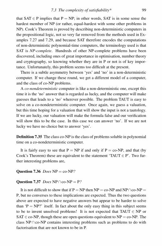
7.3 The complexity of satisfiability* 99
that SAT ∈ P implies that P = NP; in other words, SAT is in some sense thehardest member of NP (or rather, equal-hardest with some other problems inNP). Cook’s Theorem is proved by describing non-deterministic computers inthe propositional logic, not so very far removed from the methods used in Ex-amples 7.27 and 7.29, and because SAT therefore encodes the computationsof non-deterministic polynomial-time computers, the terminology used is thatSAT is NP-complete. Hundreds of other NP-complete problems have beendiscovered, including ones of great importance in optimisation, number theoryand cryptography, so knowing whether they are in P or not is of key impor-tance. Unfortunately, this problem seems too difficult at the present.
There is a subtle asymmetry between ‘yes’ and ‘no’ in a non-deterministiccomputer. If we change these round, we get a different model of a computer,and the class of co-NP problems.
A co-nondeterministic computer is like a non-deterministic one, except thistime it is the ‘no’ answer that is regarded as lucky, and the computer will makeguesses that leads to a ‘no’ wherever possible. The problem TAUT is easy tosolve on a co-nondeterministic computer. Once again, we guess a valuation,but this time hoping for a valuation that will show the input is not a tautology.If we are lucky, our valuation will make the formula false and our verificationwill show this to be the case. In this case we can answer ‘no’. If we are notlucky we have no choice but to answer ‘yes’.
Definition 7.35 The class co-NP is the class of problems soluble in polynomialtime on a co-nondeterministic computer.
It is fairly easy to see that P = NP if and only if P = co-NP, and that (byCook’s Theorem) these are equivalent to the statement ‘TAUT ∈ P’. Two fur-ther interesting problems are,
Question 7.36 Does NP = co-NP?
Question 7.37 Does NP∩ co-NP = P?
It is not difficult to show that if P = NP then NP = co-NP and NP∩co-NP =P, but no converses to these implications are expected. Thus the two questionsabove are expected to have negative answers but appear to be harder to solvethan ‘P = NP?’ itself. In fact about the only easy thing in this subject seemsto be to invent unsolved problems! It is not expected that TAUT ∈ NP orSAT ∈ co-NP, though these are open questions equivalent to NP = co-NP. Theclass NP∩ co-NP contains interesting problems such as problems to do withfactorisation that are not known to be in P.

8
Filters and ideals
8.1 Algebraic theory of boolean algebras
In this chapter we start to explore the theory of boolean algebras as an algebraictheory in its own right, in a way analogous to ring theory, say. We will seemany applications of the Completeness and Soundness Theorems proved inthe last chapter.
We start with an important definition concerning boolean algebras.
Definition 8.1 Let B, C be boolean algebras. A homomorphism from B to C isa map h: B→C such that, for all a, b ∈ B,
• h(a∨b) = h(a)∨h(b)• h(a∧b) = h(a)∧h(b)• h(�) = �• h(⊥) = ⊥• h(a′) = h(a)′
Here, ∨ and ∧, etc., are calculated inside B on the left hand side, and inside Con the right. In fact, the last condition (on complementation) is not necessaryand follows from the other four, since if those four hold then we have � =h(�) = h(a′ ∨ a) = h(a′)∨ h(a) and ⊥ = h(⊥) = h(a′ ∧ a) = h(a′)∧ h(a) soh(a′) = h(a)′ by Proposition 5.22 on the Uniqueness of Complements.
We will see several examples of homomorphisms later, but first we studyone particular homomorphism of boolean algebras that applies to all such B.
Definition 8.2 Let B be a boolean algebra. Define a boolean algebra Bop =(B, ∧op, ∨op, ′, �op, ⊥op) with the same underlying set and the same comple-mentation operation as B, by defining the other operations as follows
• x∧opy = x∨ y
100

8.1 Algebraic theory of boolean algebras 101
• x∨opy = x∧ y• �op = ⊥• ⊥op = �
Bop is a boolean algebra in its own right, called the opposite of B. The mapx �→ x′ is a homomorphism B→Bop which is also one-to-one and onto. Inother words it is an isomorphism of boolean algebras. This ‘opposite’ mapturns boolean algebras ‘upside down’ swapping � and ⊥ and reversing theorder relation. It also swaps ∧ and ∨, showing that we should expect theseoperations to have similar properties. More importantly, it shows that for everynotion in a boolean algebra there is a dual notion, in which the order is reversedand �, ⊥ and ∧, ∨ are swapped over, and proofs of propositions for one kindcarry over directly to the dual. Again, we will see plenty of examples in thischapter.
As well as being used to model propositional logic, boolean algebras areclosely related to rings. (See the exercises below for more details.) In ringtheory, the important subsets of a ring are the ideals. These are the subringswhich can be used to ‘quotient out’ the ring to get a new (and often nicer)ring. One way of understanding ideals of rings is that they are the kernels ofhomomorphisms. The same applies for boolean algebras.
Definition 8.3 Let h: B→C be a homomorphism of boolean algebras. Thenthe kernel of h is the subset kerh = {a ∈ B : h(a) = ⊥}.
Proposition 8.4 Let h: B→C be a homomorphism of boolean algebras andI = kerh. Then I satisfies: (a) if a ∈ I and b ∈ I then a∨b ∈ I; (b) if a ∈ I andb ∈ B with b � a then b ∈ I. In particular, it follows from (b) that I contains ⊥and is closed under ∧.
Proof If a ∈ I and b ∈ I then h(a) = h(b) = ⊥ so h(a∨b) = h(a)∨h(b) = ⊥,so a ∨ b ∈ I. Also, if a ∈ I and b ∈ B with b � a then h(b) = h(b ∧ a) =h(b)∧h(a) � ⊥ so h(b) = ⊥ and b ∈ I.
Definition 8.5 Let B be a boolean algebra, or more generally, a lattice. Anideal of B is a non-empty subset I ⊆ B such that for all x, y ∈ B: (a) x � y ∈ Iimplies x ∈ I; and (b) x, y ∈ I implies x∨y ∈ I. The ideal I is proper if it is notequal to the whole of B.
As you may have guessed, there is a similar dual notion obtained by replac-ing ∧, ∨ , �, ⊥ by their duals ∨, ∧ , ⊥, �. The dual notion to that of an idealis called a filter.

102 Filters and ideals
Definition 8.6 A filter of B is a non-empty subset F ⊆ B such that for allx, y ∈ B: (a) x � y ∈ F implies x ∈ F ; and (b) x, y ∈ F implies x∧ y ∈ F . It isproper if it is not equal to the whole of B.
As mentioned, filters and ideals are dual concepts. If I is an ideal thenF = {a′ : a ∈ I} is the corresponding filter, and vice versa.
The way to picture these is to think of an ideal as representing a set ofelements to be thought of as ‘negligible’, ‘small’ or ‘false’. If x � y and y is‘false’ then x should also be false as it is ‘more false’ than y. Also if x, y ∈ I areboth ‘false’ then so is x∨y or ‘x or y’. Similarly a filter is a set of elements thatcan be thought of as ‘large’ or ‘true’. If x � y, i.e. x is ‘more true’ than a truestatement y, then x should be ‘true’, and if both x, y are ‘true’ then so should‘x and y’ or x∧ y. In this picture, we should only be interested in proper idealsand proper filters, because we want to retain at least some distinction between‘true’ and ‘false’.
Another way of saying the same thing – a way that is algebraically somewhatmore sophisticated – is to say that we can factor a boolean algebra out by anideal to make everything in the ideal look like ⊥. Similarly we can factor outby a filter to make everything in the filter look like �.
Factoring out an ideal or filter has repercussions on the whole of the booleanalgebra, though. If x, y ∈ B and I is an ideal consisting of objects to be thoughtof as ‘false’ or ‘negligible’ then x and y should be regarded as equivalent mod-ulo the ideal I if the terms representing how x and y differ, i.e. the terms x∧ y′
and x′ ∧ y, are both negligible. (In the case when B is a boolean algebra ofsubsets of some set X you can think of this as saying the set differences x \ yand y \ x are both negligible.)
Exercise 8.7 (For those who have read Section 5.3.) Switching when nec-essary between B as a boolean algebra and B as a boolean ring, the differ-ence between x and y is x − y, or (as B has characteristic 2), x + y. Butx + y = (x∧ y′)∨ (x′ ∧ y), and so x− y ∈ I if and only if (x∧ y′)∨ (x′ ∧ y) ∈ I,which is the case if and only if both (x∧y′), (x′ ∧y)∈ I, since ideals are closedunder ∨.
Dually, x and y are equivalent modulo the filter F if x∧ y′ and x′ ∧ y are inthe corresponding ideal, i.e. (x∧y′)′ ∈ F and (x′ ∧y)′ ∈ F , which is equivalentto saying that both x′ ∨ y ∈ F and x∨ y′ ∈ F . (You can think of this as sayingthat the filter makes both implications x→ y and y→ x true.)
Definition 8.8 Let B be a boolean algebra and I ⊆ B an ideal. Then B/I is the

8.1 Algebraic theory of boolean algebras 103
set of equivalence classes for the equivalence relation
a ∼ b if and only if (a′ ∧b) ∈ I and (a∧b′) ∈ I.
Similarly, if F ⊆ B a filter. Then B/F is the set of equivalence classes for theequivalence relation
a ∼ b if and only if (a∨b′) ∈ F and (a′ ∨b) ∈ F .
The quotients B/I and B/F are made into a boolean algebra by defining
• � = [�] = F• ⊥ = [⊥] = I• [a]∨ [b] = [a∨b]• [a]∧ [b] = [a∧b]• [a]′ = [a′]
for each a, b ∈ B, where [x] denotes the ∼-equivalence class of x.
Proposition 8.9 In each of these cases, ∼ is an equivalence relation, theoperations of ∨, ∧ and ′ on the quotient are well defined (i.e. do not depend onthe choice of the representative of the equivalence class used to define them)and satisfy the axioms for a boolean algebra. The quotient algebra is proper(i.e. not degenerate) if and only if the ideal (or filter) used is proper.
Proof This is a long detailed check against the axioms. We will do sometypical steps, including the more difficult ones, and leave the remaining partsas an exercise for the more energetic students.
To see that ∼ is an equivalence, note that x ∼ x as ⊥= x∧x′ = x′ ∧x ∈ I. Thesymmetry axiom is obvious. For transitivity, suppose x∧ y′, x′ ∧ y, y∧ z′, y′ ∧ zare all in I. Then
x∧ z′ = (x∧ z′ ∧ y)∨ (x∧ z′ ∧ y′) = (x∧ z′)∧ ((y∧ z′)∨ (x∧ y′))
which is in I as (y∧ z′), (x∧ y′) ∈ I and I is closed downwards and under ∨.Similarly for x′ ∧ z.
The operations on B/I are well defined. For example if x1 ∼ x2 and y1 ∼ y2
then x1 ∧ x2′, x1
′ ∧ x2 and y1 ∧ y2′, y1
′ ∧ y2 are all in I. Thus (x1 ∧ y1)∧ (x2 ∧y2)
′ = x1 ∧y1 ∧ (x2′ ∨y2
′) = (x1 ∧y1 ∧x2′)∨ (x1 ∧y1 ∧y2
′) = (x1 ∧y1)∧ ((x1 ∧x2
′)∨(y1∧y2′)) which is in I by the closure properties of I. All other cases are
similar.Checking the axioms for a boolean algebra is now easy. (I suggest the easiest
way is to check against the properties in Proposition 5.15; see also Proposition5.16.) To check that the quotient is proper, it suffices to check that it is not thecase that �∼⊥. But if �∼⊥ then �=�∧⊥′ ∈ I, so I = B is not proper.

104 Filters and ideals
In the sequel, I will tend to concentrate on filters rather than ideals since (beingan optimist) I prefer to focus on true statements rather than false ones, but aswe have seen these ideas are interchangeable. (Is this boolean algebra half-trueor half-false?) Pessimists can easily translate what I have to say to ideals usingduality.
The next lemma presents a useful way of making a new filter from an oldone by adding a new element x to the filter and closing the resulting set under� and ∧.
Lemma 8.10 Let B be a boolean algebra, x ∈ B, and F ⊆ B a filter of B. Then
G = {g : g � x∧ f , for some f ∈ F}is a filter containing both x and all elements of F, and is in fact the least suchfilter. The filter G is a proper filter except when x′ ∈ F.
Proof Checking that G is a filter is routine. If g ∈ G and h � g then it is clearthat h ∈ G from the definition. If g1 � x∧ f1 and g2 � x∧ f2 with f1, f2 ∈ Fthen g1 ∧ g2 � (x∧ f1)∧ (x∧ f2) = x∧ ( f1 ∧ f2) and f1 ∧ f2 ∈ F since F is afilter.
For the final part, suppose that G is not proper. Then ⊥∈ G so ⊥� x∧ f forsome f ∈ F so f � x′. Hence x′ ∈ F as F is a filter.
Our set BT(X) of boolean terms over X is close to being a boolean algebra inits own right. It has operations of ∧, ∨ and complementation given by t, s �→(t ∧ s), t, s �→ (t ∨ s), t �→ ¬ t, for terms t, s ∈ BT(X). The problem is thatcertain distinct terms should be ‘equal’. For example, for x, (x∧ x) and (x∨ x)ought to be equal to each other as elements of the boolean algebra but are infact distinct terms. The solution is once again to use an equivalence relation.
Lemma 8.11 Let X be a set. Then we may define an equivalence relation ∼on BT(X) by
t ∼ s if and only if t � s and s� t.
The set of equivalence classes [t] of BT(X) forms a boolean algebra when wedefine
• [t] � [s] if and only if t � s• [t]∧ [s] = [(t ∧ s)]• [t]∨ [s] = [(t ∨ s)]• [t]′ = [¬ t]• � = [�]
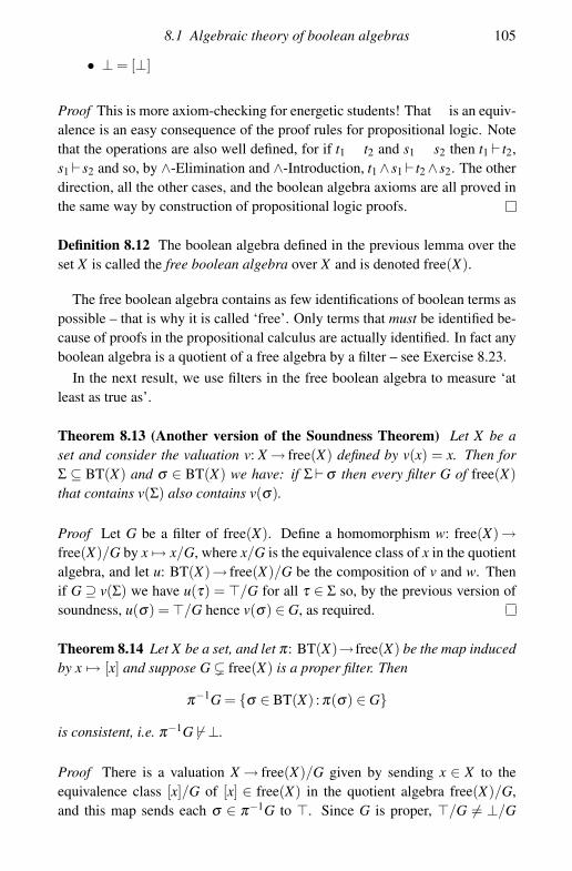
8.1 Algebraic theory of boolean algebras 105
• ⊥ = [⊥]
Proof This is more axiom-checking for energetic students! That ∼ is an equiv-alence is an easy consequence of the proof rules for propositional logic. Notethat the operations are also well defined, for if t1 ∼ t2 and s1 ∼ s2 then t1 � t2,s1 � s2 and so, by ∧-Elimination and ∧-Introduction, t1 ∧ s1 � t2 ∧ s2. The otherdirection, all the other cases, and the boolean algebra axioms are all proved inthe same way by construction of propositional logic proofs.
Definition 8.12 The boolean algebra defined in the previous lemma over theset X is called the free boolean algebra over X and is denoted free(X).
The free boolean algebra contains as few identifications of boolean terms aspossible – that is why it is called ‘free’. Only terms that must be identified be-cause of proofs in the propositional calculus are actually identified. In fact anyboolean algebra is a quotient of a free algebra by a filter – see Exercise 8.23.
In the next result, we use filters in the free boolean algebra to measure ‘atleast as true as’.
Theorem 8.13 (Another version of the Soundness Theorem) Let X be aset and consider the valuation v: X → free(X) defined by v(x) = x. Then forΣ ⊆ BT(X) and σ ∈ BT(X) we have: if Σ�σ then every filter G of free(X)that contains v(Σ) also contains v(σ).
Proof Let G be a filter of free(X). Define a homomorphism w: free(X)→free(X)/G by x �→ x/G, where x/G is the equivalence class of x in the quotientalgebra, and let u: BT(X)→ free(X)/G be the composition of v and w. Thenif G ⊇ v(Σ) we have u(τ) = �/G for all τ ∈ Σ so, by the previous version ofsoundness, u(σ) = �/G hence v(σ) ∈ G, as required.
Theorem 8.14 Let X be a set, and let π: BT(X)→ free(X) be the map inducedby x �→ [x] and suppose G � free(X) is a proper filter. Then
π−1G = {σ ∈ BT(X) : π(σ) ∈ G}
is consistent, i.e. π−1G � �⊥.
Proof There is a valuation X → free(X)/G given by sending x ∈ X to theequivalence class [x]/G of [x] ∈ free(X) in the quotient algebra free(X)/G,and this map sends each σ ∈ π−1G to �. Since G is proper, �/G �= ⊥/G

106 Filters and ideals
in free(X)/G, so this valuation does not send ⊥ ∈ BT(X) to ⊥ in free(X)/G.Therefore π−1G is consistent by soundness.
Definition 8.15 Let F be a filter in a boolean algebra B. We say that F is primeif it is proper and whenever a, b ∈ B with a∨b ∈ F then either a or b is in F .
Dually, an ideal I is prime if it is proper and whenever a, b ∈ B with a∧b ∈ Ithen either a or b is in I.
Proposition 8.16 Let B be a boolean algebra and F � B a proper filter. Thenthe following are equivalent.
• F is maximal, i.e. there is no filter G with F � G � B.• F is prime.• F has the property that for all x ∈ B either x ∈ F or x′ ∈ F.• B/F is isomorphic to the two-element boolean algebra {�, ⊥}.
Proof If F is maximal and a∨b∈F with neither a, b∈F then, by Lemma 8.10,we may extend F to the filters Ga = {g : g � a∧ f for some f ∈ F} and Gb ={g : g � b∧ f for some f ∈ F} and these contain a, b respectively; hence theyare improper by the maximality of F . Therefore ⊥ � a∧ f and ⊥ � b∧g forsome f , g ∈ F , so ⊥� (a∧ f )∨ (b∧g) = (a∨b)∧ ( f ∨b)∧ (a∨g)∧ ( f ∨g) ∈F , hence F is also not proper, contradicting assumption. So F is maximalimplies that F is prime.
If F is prime then x∨ x′ = � ∈ F so one of x, x′ ∈ F , so F has the thirdproperty listed in the proposition.
If F has the property that one of x, x′ ∈ F for each x, then the equivalenceclass x/F of x is either F itself (if x ∈ F) or {x′ : x ∈ F} (if x′ ∈ F) as you maycheck. Therefore there are only two such equivalence classes and B/F is thetwo-element boolean algebra.
If B/F is isomorphic to {�, ⊥} then F = {x ∈ B : x/F = �/F} and so fora filter G with F � G ⊆ B we have x ∈ G for some x/F = ⊥/F . It followsfrom the definition of the equivalence class x/F that x∨ f =⊥ for some f ∈ Fi.e. G = B.
Maximal proper filters are usually called ultrafilters. The previous propositionshows that this notion of ultrafilter coincides exactly with prime filter. Thefollowing theorem stating that ultrafilters exist is an important consequenceof Zorn’s Lemma. It is normally known as the Prime Ideal Theorem, and weshall stick with this convention, despite the fact that we shall state the resultin its equivalent form concerning filters. It is in fact just another form of theCompleteness Theorem for propositional logic.
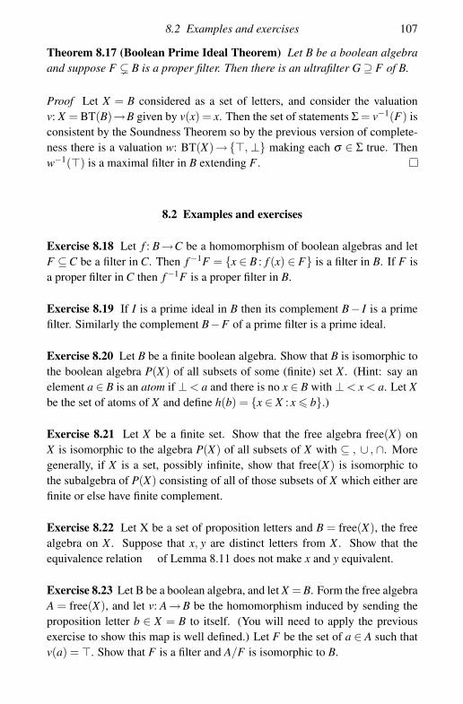
8.2 Examples and exercises 107
Theorem 8.17 (Boolean Prime Ideal Theorem) Let B be a boolean algebraand suppose F � B is a proper filter. Then there is an ultrafilter G ⊇ F of B.
Proof Let X = B considered as a set of letters, and consider the valuationv: X = BT(B)→B given by v(x) = x. Then the set of statements Σ = v−1(F) isconsistent by the Soundness Theorem so by the previous version of complete-ness there is a valuation w: BT(X)→{�, ⊥} making each σ ∈ Σ true. Thenw−1(�) is a maximal filter in B extending F .
8.2 Examples and exercises
Exercise 8.18 Let f : B→C be a homomorphism of boolean algebras and letF ⊆C be a filter in C. Then f−1F = {x ∈ B : f (x) ∈ F} is a filter in B. If F isa proper filter in C then f−1F is a proper filter in B.
Exercise 8.19 If I is a prime ideal in B then its complement B− I is a primefilter. Similarly the complement B−F of a prime filter is a prime ideal.
Exercise 8.20 Let B be a finite boolean algebra. Show that B is isomorphic tothe boolean algebra P(X) of all subsets of some (finite) set X . (Hint: say anelement a ∈ B is an atom if ⊥ < a and there is no x ∈ B with ⊥ < x < a. Let Xbe the set of atoms of X and define h(b) = {x ∈ X : x � b}.)
Exercise 8.21 Let X be a finite set. Show that the free algebra free(X) onX is isomorphic to the algebra P(X) of all subsets of X with ⊆ , ∪ , ∩. Moregenerally, if X is a set, possibly infinite, show that free(X) is isomorphic tothe subalgebra of P(X) consisting of all of those subsets of X which either arefinite or else have finite complement.
Exercise 8.22 Let X be a set of proposition letters and B = free(X), the freealgebra on X . Suppose that x, y are distinct letters from X . Show that theequivalence relation ∼ of Lemma 8.11 does not make x and y equivalent.
Exercise 8.23 Let B be a boolean algebra, and let X = B. Form the free algebraA = free(X), and let v: A→B be the homomorphism induced by sending theproposition letter b ∈ X = B to itself. (You will need to apply the previousexercise to show this map is well defined.) Let F be the set of a ∈ A such thatv(a) = �. Show that F is a filter and A/F is isomorphic to B.

108 Filters and ideals
Exercise 8.24 (For those who have read Section 5.3 on the algebra of Boole.)Let R be a boolean ring and B the boolean algebra corresponding to it. Showthat I ⊆ R is an ideal of R in the sense of ring theory (i.e. is non-empty, isclosed under + and satisfies xy ∈ I whenever one of x or y is in R) if and onlyif I is an ideal of B in the sense of boolean algebras.
8.3 Tychonov’s Theorem*
The main theorem of this chapter was the Boolean Prime Ideal Theorem, thefact that every proper filter in a boolean algebra can be extended to an ul-trafilter, i.e. a maximal and hence prime proper filter. Ultrafilters have manyapplications in mathematics, including to logic itself, and to infinitary combi-natorics.
One nice application of ultrafilters is their use in proving Tychonov’s The-orem, that an arbitrary product of compact topological spaces is compact. Wesay an open cover Ui (i ∈ I) of a topological space X is a family of open setswhose union is the whole of X , and the closure of a set A⊆ X is the set of x ∈ Xsuch that every non-empty open U containing x also contains some a ∈ A. Theclosure of A is denoted A. We start with a characterisation of compact topo-logical spaces.
Proposition 8.25 Let X be a topological space, and B = P(X) the booleanalgebra of subsets of X. Then the following are equivalent.
• Any open cover Ui (i∈ I) of X has a finite subcover Uin (n = 0, 1, . . ., k).• For any proper filter F ⊆B the intersection
⋂{A : A ∈ F
}is non-empty.
Proof For one direction, suppose F ⊆ B is a filter. Then U ={
Ac : A ∈ F}
,the set of complements of closures of A ∈ F , is a collection of open sets. If⋂{
A : A ∈ F}
= ∅ then there is no x ∈ X in all the A (A ∈ F), so U is an opencover of X . Therefore there are A1, . . ., An ∈ F such that A1
c ∪ . . .∪Anc = X
hence A1 ∩ . . .∩An = ∅ hence A1 ∩ . . .∩An = ∅, so F is not proper.For the other direction, let Ui (i ∈ I) be an open cover of X with no finite
subcover. Then the Ui generate a proper filter,
F ={
A : A ⊇Uci1 ∩ . . .∩Uc
in , some n, i1, . . ., in}
,
and⋂{
A : A ∈ F}
=⋂{Uc
i : i ∈ I} = ∅ as the Ui cover X .
Definition 8.26 A topological space X satisfying either of the conditions inthe last proposition is said to be compact.
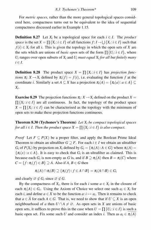
8.3 Tychonov’s Theorem* 109
For metric spaces, rather than the more general topological spaces consid-ered here, compactness turns out to be equivalent to the idea of sequentialcompactness discussed earlier in Example 1.15.
Definition 8.27 Let Xi be a topological space for each i ∈ I. The productspace is the set X = ∏{Xi : i ∈ I} of all functions f : I→⋃{Xi : i ∈ I} such thatf (i) ∈ Xi for all i. This is given the topology in which the open sets of X arethe sets which are unions of basic open sets of the form ∏{Ui : i ∈ I}, whereUi ranges over open subsets of Xi and Ui must equal Xi for all but finitely manyi ∈ I.
Definition 8.28 The product space X = ∏{Xi : i ∈ I} has projection func-tions πi: X →Xi defined by πi( f ) = f (i), i.e. evaluating the function f at thecoordinate i. Similarly a set A ⊆ X has a projection πi(A) = {πi(a) : a ∈ A} ⊆Xi.
Exercise 8.29 The projection functions πi: X →Xi defined on the product X =∏{Xi : i ∈ I} are all continuous. In fact, the topology of the product spaceX = ∏{Xi : i ∈ I} can be characterised as the topology with the minimum ofopen sets to make these projection functions continuous.
Theorem 8.30 (Tychonov’s Theorem) Let Xi be compact topological spacesfor all i ∈ I. Then the product space X = ∏{Xi : i ∈ I} is also compact.
Proof Let F ⊆ P(X) be a proper filter, and apply the Boolean Prime IdealTheorem to obtain an ultrafilter G ⊇ F . For each i ∈ I we obtain an ultrafilterGi of P(Xi) by projection on Xi defined by Gi = {πi(A) : A ∈ G} where πi(A) ={πi(x) : x ∈ A}. It is easy to check that Gi is an ultrafilter as claimed. This isbecause each Gi is non-empty as G is, and if B ⊇ πi(A) then B = πi(C) whereC = { f : πi( f ) ∈ B} ⊇ A. Also if A, B ∈ G then
πi(A)∩πi(B) ⊇ {πi( f ) : f ∈ A∩B} = πi(A∩B) ∈ Gi
and clearly ∅ �∈ Gi since ∅ �∈ G.By the compactness of Xi, there is for each i some a ∈ Xi in the closure of
each πi(A) ∈ Gi. Using the Axiom of Choice we select one such ai ∈ Xi foreach i, and define a ∈ X to be the function a: i �→ ai. Then it remains to checkthat a ∈ A for each A ∈ G. That is, we need to show that if U ⊆ X is an openneighbourhood of a then U ∩A �= ∅. As open sets in X are unions of basicopen sets, it suffices to prove this in the case when U = ∏{Ui : i ∈ I} is such abasic open set. Fix some such U and consider an index i. Then as ai ∈ πi(A)
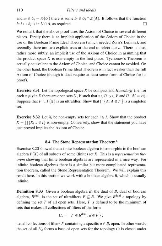
110 Filters and ideals
and ai ∈Ui = πi(U) there is some bi ∈Ui ∩πi(A). It follows that the functionb: i �→ bi is in U ∩A, as required.
We remark that the above proof uses the Axiom of Choice in several differentplaces. Firstly there is an implicit application of the Axiom of Choice in theuse of the Boolean Prime Ideal Theorem (which needed Zorn’s Lemma); andsecondly there are two explicit uses at the end to select our a. There is also,rather more subtly, an implicit use of the Axiom of Choice in assuming thatthe product space X is non-empty in the first place. Tychonov’s Theorem isactually equivalent to the Axiom of Choice, and Choice cannot be avoided. Onthe other hand, the Boolean Prime Ideal Theorem is in fact weaker than the fullAxiom of Choice (though it does require at least some form of Choice for itsproof).
Exercise 8.31 Let the topological space X be compact and Hausdorff (i.e. foreach x �= y in X there are open sets U , V such that x ∈U , y∈V and U ∩V = ∅).Suppose that F ⊆ P(X) is an ultrafilter. Show that
⋂{A : A ∈ F
}is a singleton
set.
Exercise 8.32 Let Xi be non-empty sets for each i ∈ I. Show that the productX = ∏{Xi : i ∈ I} is non-empty. Conversely, show that the statement you havejust proved implies the Axiom of Choice.
8.4 The Stone Representation Theorem*
Exercise 8.20 showed that a finite boolean algebra is isomorphic to the booleanalgebra P(X) of all subsets of some (finite) set X . This is a representation the-orem showing that finite boolean algebras are represented in a nice way. Forinfinite boolean algebras there is a similar but more complicated representa-tion theorem, called the Stone Representation Theorem. We will explain thisresult here. In this section we work with a boolean algebra B, which is usuallyinfinite.
Definition 8.33 Given a boolean algebra B, the dual of B, dual of booleanalgebra, Bdual, is the set of ultrafilters F ⊆ B. We give Bdual a topology bydefining the set T of all open sets. Here, T is defined to be the minimum ofsets that makes all collections of filters of the form
Ua ={
F ∈ Bdual : a ∈ F}
,
i.e. all collections of filters F containing a specific a ∈ B, open. In other words,the set of all Ua forms a base of open sets for the topology (it is closed under

8.4 The Stone Representation Theorem* 111
intersections because Ua ∩Ub = Ua∧b) and T is defined to be the set of allU ⊆ Bdual which are a union of sets of the form Ua. We call Bdual with thistopology the dual space of B.
Definition 8.34 A topological space X is totally disconnected if for all x, y∈Xwith x �= y there are open U , V ⊆ X with x ∈ U , y ∈ V and X = U ∪V is adisjoint union of the two sets.
Proposition 8.35 The topological space Bdual is a compact totally discon-nected topological space, in which the clopen subsets (i.e. sets which are bothclosed and open) are exactly the sets of the form Ua for a ∈ B.
Proof This is an application of the Boolean Prime Ideal Theorem. We start byproving compactness.
Let {Ui : i ∈ I} be an open cover of Bdual. We must show that there is afinite subcover. Each Ui is a union of basic open sets, so there is a cover{Ua : a ∈ A} for some A ⊆ B such that each Ua (a ∈ A) is a subset of some Ui.It suffices therefore to show that there is a finite subcover of {Ua : a ∈ A}. Weshall assume, to get a contradiction, that there is no such subcover.
Consider the filter
F ={
x ∈ B : x � a1′ ∧ . . .∧ak
′, k ∈ N, a1, . . ., ak ∈ A}
.
This is clearly a filter. It is also proper since if ⊥ ∈ F then a1′ ∧ . . .∧ ak
′ =⊥ for some k and some a1, . . ., ak ∈ A; we show that this would imply thatUa1 ∪ . . .∪Uak = Bdual. If G ∈ Bdual, so G ⊆ B is a (proper) ultrafilter andG �∈Uai for each i then ai �∈ G for each i (by the definition of Uai ) so ai
′ ∈ G foreach i, as G is an ultrafilter. It would follow that ⊥= a1
′ ∧ . . .∧ak′ ∈ G, which
is impossible.Now, since F is a proper filter of B it extends to an ultrafilter F ⊆ G ∈ Bdual.
But by construction G �∈ Ua for each a ∈ A, as a′ ∈ F ⊆ G and therefore a �∈G, otherwise G would contain a∧ a′ = ⊥. Thus {Ua : a ∈ A} is not in fact acover of Bdual, and this is our required contradiction completing the proof ofcompactness.
The other properties now follow more easily. To see that Bdual is totallydisconnected, note first that Ua ∪Ua′ = Bdual is a disjoint two-set cover of Bdual
for each a ∈ B. This is because each ultrafilter G of B contains exactly oneof a, a′. Thus each Ua is clopen, and if F , G ∈ Bdual are distinct there is somea ∈ F \ G or b ∈ G \ F ; in the first case we have F ∈Ua and G ∈Ua′ , and in thesecond case F ∈Ub′ and G ∈Ub. This shows that Bdual is totally disconnected.
Now suppose U ⊆ Bdual is clopen. We want to show U = Ua for some a ∈ B.

112 Filters and ideals
As U is open there are Uai (i ∈ I) such that U =⋃{
Uai : i ∈ I}
, and as Uc isopen there are Ub j ( j ∈ J) such that Uc =
⋃{Ub j : j ∈ J
}. Thus the Uai and Ub j
form an open cover of Bdual, and by compactness there is a finite subcover. Inparticular U = Ua1 ∪ . . .∪Uak for some a1, . . ., ak ∈ B. It follows that U = Ua
where a = a1 ∨ . . .∨ ak, for given an ultrafilter G ∈ Bdual we have: if G ∈ Ua
then some ai ∈ G (for if ai �∈ G for all i then ai′ ∈ G as G is an ultrafilter, so
⊥= (a1∨ . . .∨ak)∨(a1′ ∧ . . .∧ak
′)∈ G which is impossible) hence G ∈Uai soG ∈U ; and conversely, if G ∈U then ai ∈ G for some i so a = a1∨ . . .∨ak � ai
is also in G. Thus the clopen sets are precisely the basic open sets.
The interesting thing about clopen sets is that finite unions and intersectionsof clopen sets are clopen, as are complements of clopen sets. In other words,the collection of clopen subsets of a topological space forms a boolean algebrawith the usual ⊆ relation, and ∪, ∩. This now gives the promised representa-tion theorem.
Theorem 8.36 (Stone Representation Theorem) Let B be a boolean algebraand Bdual its dual space. Then the map
a �→ Ua
is an isomorphism from the boolean algebra B to the boolean algebra of clopensubsets of Bdual.
Proof Most of the ideas have already been presented in the last proposition,and we only need to tie some loose ends. In particular, the map a �→ Ua isa homomorphism of boolean algebras from B to the algebra of clopen sets inBdual.
To see Ua∧b = Ua ∩Ub, take an ultrafilter G and observe a∧ b ∈ G impliesa ∈ G and b ∈ G as a, b � a ∧ b and conversely a ∈ G and b ∈ G impliesa∧b ∈ G as G is closed under ∧.
To see Ua∨b = Ua ∪Ub, observe a∨b ∈ G implies a ∈ G or b ∈ G as G is anultrafilter and the alternative would be a′ ∈ G and b′ ∈ G. Conversely a ∈ G orb ∈ G implies a∨b ∈ G as a∨b � a, b.
That Ua′ = Uac has already been noted, as Ua ∪Ua′ = Bdual is a disjoint
union. Also U⊥ = ∅ and U� = Bdual as every ultrafilter G contains �, andnone contains ⊥. This shows a �→ Ua is a homomorphism of boolean algebras.
Finally, this homomorphism is onto, since every clopen set is Ua for somea, and one-to-one since if a �= b then F = {x : x � a∧b′} is a proper filter(proper because a∧b′ = ⊥ implies a = b) and so is contained in an ultrafilterG ∈Ua \ Ub.

8.4 The Stone Representation Theorem* 113
If we now take one step back we may see that this correspondence between theboolean algebra and its dual space is much deeper and more powerful.
Definition 8.37 Say a topological space X is a Stone space if it is compact andtotally disconnected.
Let BOOL denote the class of all boolean algebras and STONE the classof all Stone spaces. Then the Stone Representation Theorem uses two impor-tant maps, D: BOOL→STONE, taking B to S(B) = Bdual, and E: STONE→BOOL, taking X to the boolean algebra B(X) = Xclopen of clopen subsets ofX . The Stone Theorem says that B(S(B)) is isomorphic to B. In fact a similarresult holds the other way round too, and the maps D and E are inverse to eachother.
Theorem 8.38 Let X be a Stone space, B = Xclopen the boolean algebra ofclopen subsets of X, and Y = Bdual the dual space of B. Then X and Y arehomeomorphic.
Proof We must define a map X →Y and show it is one-to-one, onto, continu-ous, and with continuous inverse. Given x ∈ X we define
Dx = {U ⊆ X :U clopen, x ∈U} .
The set Dx is a set of clopen subsets of X , hence a subset of B and our mapwill be x �→ Dx. For this map to be well defined as a map X →Y we need tocheck that Dx is indeed an ultrafilter. But if U , V ⊆ X are any clopen sets andx ∈ U and x ∈ V then x ∈ U ∩V and U ∩V is clopen. Similarly if x ∈ U ⊆ Vthen x ∈ V . Thus Dx is a filter. It is proper as it does not contain ∅ and anultrafilter because if U is any clopen set then Uc is clopen and x is in exactlyone of U , Uc, hence exactly one of U , Uc is in Dx.
To check that x �→ Dx is one-to-one, suppose x �= y are elements of X . Thenby total disconnectedness there are disjoint clopen U , V ⊆ X such that x ∈U ,y ∈V and X = U ∩V . So U ∈ Dx and V ∈ Dy and Dx �= Dy.
For the onto property, we use compactness. Let G ⊆ B = Xclopen be anultrafilter. Then by compactness and Proposition 8.25 there is some x in theintersection
⋂{U :U ∈ G
}. As each U ∈ G is already closed, we may write
this more simply as x ∈ ⋂G. Now let U ⊆ X be clopen. Then X = U ∪Uc is
a disjoint union of clopen sets and G contains exactly one of U , Uc as it is anultrafilter. Since x ∈ ⋂
G, G must contain whichever of U , Uc that contains x,and hence G = Dx.
For continuity, suppose U ⊆ Y is basic open, of the form U = UV , where

114 Filters and ideals
V ∈ B, i.e. V ⊆ X is clopen. Then U = {Dx :V ∈ Dx} and the inverse image ofU under x �→ Dx is just V , which is open. Similarly, every open set of a totallydisconnected space is a union of clopen sets. If V ⊆ X is clopen then the imageof V under x �→ Dx is {Dx : x ∈V} which equals {Dx :V ∈ Dx}, a clopen setin Y .
For our final refinement of these ideas, we can consider the classes BOOL andSTONE together with their familiar notion of ‘homomorphisms’. (In otherwords, we consider BOOL and STONE as categories, though we shall notin fact need or use any terminology from category theory in this book.) ForA, B ∈ BOOL, the notion of ‘homomorphism’ is that of ordinary homomor-phisms A → B of boolean algebras. For X , Y ∈ STONE the correspondingnotion of ‘homomorphism’ is that of a continuous map X →Y . Then, not onlydo boolean algebras and their Stone-space duals correspond, but so also dohomomorphisms between them – except that in the correspondence of homo-morphisms the direction of the maps must be reversed. (It is this reversal ofthe direction of maps that is characteristic of ‘duality’ and the reason for call-ing Bdual the ‘dual’ of B in the first place.) Specifically, we have the followingtheorem.
Theorem 8.39 (a) Let A, B ∈ BOOL be boolean algebras and let h: A→Bbe a homomorphism of boolean algebras. Then there is a continuous mapS(h): S(B)→S(A) from the dual S(B) = Bdual of B to the dual S(A) = Adual ofA given by a ∈ S(h)(y) if and only if h(a) ∈ y. Furthermore, if h is one-to-onethen S(h) is onto, and if h is onto then S(h) is one-to-one.
(b) Let X , Y ∈ STONE be Stone spaces and θ : X →Y a continuous map.Then there is a homomorphism B(θ): B(Y )→B(X) from the boolean algebraB(Y ) = Y clopen of clopen sets in Y to the boolean algebra B(X) = Xclopen ofclopen sets in X given by a ∈ θ(y) if and only if B(θ)(a) ∈ y. Furthermore, ifθ is one-to-one then B(θ) is onto, and if θ is onto then B(θ) is one-to-one.
Proof (a) Given an ultrafilter G ⊆ B define θ(G) = {a ∈ A : h(a) ∈ G}. Thisis a proper filter because: ⊥ �∈ θ(G) since h(⊥) = ⊥ �∈ G; if a, b ∈ θ(G)then h(a), h(b) ∈ G so h(a∧ b) = h(a)∧ h(b) ∈ G so a∧ b ∈ θ(G); and ifa � b∈ θ(G) then h(a) � h(b)∈G so h(a)∈G and a∈ θ(G). It is an ultrafilterbecause, given a, either h(a)∈G or h(a′) = h(a)′ ∈G. θ = S(h) is the requiredmap S(B)→S(A).
To check θ is continuous consider a basic open Ua = {H ⊆ A : a ∈ H} ⊆Adual. Then θ(G) ∈ Ua if and only if a ∈ θ(G), which holds if and only ifh(a) ∈ G, so θ−1Ua = Uh(a) is open.

8.4 The Stone Representation Theorem* 115
Given H ⊆ A let G = {h(a) : a ∈ H} so H ⊆ {a ∈ A : h(a) ∈ G}, and if h isone-to-one then for each a∈H there is a unique b∈G such that b = h(a), henceθ is onto. If h is onto and G1, G2 are such that θ(G1) = {a ∈ A : h(a) ∈ G1} ={a ∈ A : h(a) ∈ G2}= θ(G2) then for each b ∈ G1 there is a ∈ A with b = h(a)so a ∈ θ(G1) = θ(G2) hence b = h(a) ∈ G2. Thus by symmetry G1 = G2 andθ is one-to-one.
(b) Given X , Y ∈ STONE and continuous θ : X →Y we let h(U) be the set{x ∈ X : θ(x) ∈U} for a clopen U ⊆ Y . This is clopen in X by the continuityof θ and a similar amount of straightforward axiom-checking shows that h isa homomorphism of boolean algebras, is one-to-one if θ is onto, and is onto ifθ is one-to-one. Thus B(θ) = h is the required map.

9
First-order logic
9.1 First-order languages
Propositional logic is the logic of statements that can be true or false, or takesome value in a boolean algebra. The logic of most mathematical argumentsinvolves more than just this: it involves mathematical objects from one or otherdomain, such as the set of natural numbers, real numbers, complex numbers,etc. If we introduce such objects into our formal system for proof we get whatis known as first-order logic, or predicate logic.
As for any of our other logics, first-order logic would not be so interestingif it was just a system for writing and mechanically checking formal proofsfor one particular domain of mathematical work. But fortunately it can beinterpreted in a rather general class of mathematical structures and the theoryof these structures is a sort of generalised algebraic theory that applies equallywell to groups, rings, fields, and many other familiar structures, so first-orderlogic can be applied to a wide range of mathematical subject areas.
There are Completeness and Soundness Theorems for first-order logic too.In a similar way to the Completeness and Soundness Theorems we have al-ready seen, they can be read as stating the correctness and adequacy of ourlogical system, or as much more interesting constructive statements that en-able new structures to be created and analysed.
We will start here by discussing the idea of first-order language, and thesorts of things that can (and cannot) be expressed in first-order logic. Later on,we will give some rules for a proof system for this logic. The rules we givewill be precise versions of logical manoeuvres familiar from many informalarguments or proofs, and will build on the proof system for the propositionalcalculus given earlier.
Consider for the moment building a theory of the reals R. We will wantto talk about specific real numbers, so will need variables to represent reals.
116

9.1 First-order languages 117
We also require symbols for special real numbers such as 0 or 1. We willwant to say when two real numbers are equal, so we will need the symbol =for equality. We also need to combine real numbers with familiar functionssuch as x �→ −x and (x, y) �→ x+ y, etc., so we will need symbols to representthese. We may need to compare two real numbers and determine which is thegreater. A symbol for the < relation is necessary here. Finally, we need twospecial symbols ∀ and ∃ (called quantifiers) to represent the phrases ‘for all. . . ’ and ‘there exists . . . ’ common in mathematical arguments. If we put allof this together we have a first-order language for the real numbers. Thereare similar first-order languages for groups, posets, boolean algebras, etc. Thenext definition brings together all of these into one general framework.
Definition 9.1 A first-order language consists of the following symbols:
• ∧, ∨ , ¬ , �, ⊥ for propositional logic;• an infinite set of variables, x, y, z, . . .;• the symbols ‘=’, ‘∀’, ‘∃’;• a (possibly empty) set of constant symbols, such as 0, 1;• a (possibly empty) set of function symbols, such as +, ×, −;• a (possible empty) set of relation symbols, such as <;• the punctuation symbols ‘(’, ‘)’ and ‘, ’.
The logical symbols of a first-order language are ∧, ∨ , ¬ , �, ⊥, = , ∀, ∃;all the first-order languages we consider have all of these as well as variablesand punctuation symbols. (Countably infinitely many variables is always suf-ficient.) The remaining symbols are special to the particular language and arecalled non-logical symbols. Thus we can specify a first-order language by giv-ing the constant, relation and function symbols and taking the other symbolsfor granted. For example we may discuss ‘the first-order language for the realswith 0, 1, +, ×, −, <’.
Of course, a language is more than just a collection of symbols. We needto say how these symbols are combined and what the resulting strings of sym-bols (also called expressions or statements) mean. From the point of view ofexperts (or pedants) my explanation of how this is done will be very informal,relegating the more formal details to a discussion elsewhere. For beginners,the discussion that I do give will be quite complicated enough, especially aswe are working in sufficient generality to apply the ideas to such a wide rangeof mathematical topics. Fortunately, the syntactical constructions and their in-tended meanings by and large follow normal mathematical usage anyway. Myadvice to a beginner is to read and write these expressions in as natural a wayas possible, and the likelihood is that you will be right.
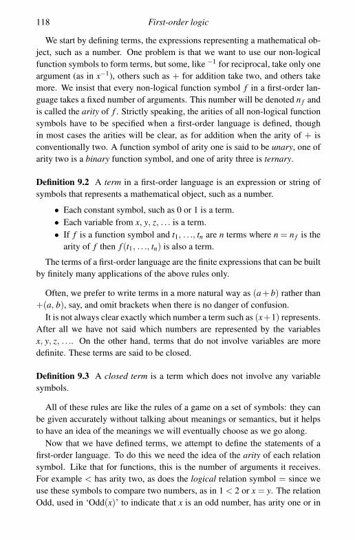
118 First-order logic
We start by defining terms, the expressions representing a mathematical ob-ject, such as a number. One problem is that we want to use our non-logicalfunction symbols to form terms, but some, like −1 for reciprocal, take only oneargument (as in x−1), others such as + for addition take two, and others takemore. We insist that every non-logical function symbol f in a first-order lan-guage takes a fixed number of arguments. This number will be denoted n f andis called the arity of f . Strictly speaking, the arities of all non-logical functionsymbols have to be specified when a first-order language is defined, thoughin most cases the arities will be clear, as for addition when the arity of + isconventionally two. A function symbol of arity one is said to be unary, one ofarity two is a binary function symbol, and one of arity three is ternary.
Definition 9.2 A term in a first-order language is an expression or string ofsymbols that represents a mathematical object, such as a number.
• Each constant symbol, such as 0 or 1 is a term.• Each variable from x, y, z, . . . is a term.• If f is a function symbol and t1, . . ., tn are n terms where n = n f is the
arity of f then f (t1, . . ., tn) is also a term.
The terms of a first-order language are the finite expressions that can be builtby finitely many applications of the above rules only.
Often, we prefer to write terms in a more natural way as (a+b) rather than+(a, b), say, and omit brackets when there is no danger of confusion.
It is not always clear exactly which number a term such as (x+1) represents.After all we have not said which numbers are represented by the variablesx, y, z, . . .. On the other hand, terms that do not involve variables are moredefinite. These terms are said to be closed.
Definition 9.3 A closed term is a term which does not involve any variablesymbols.
All of these rules are like the rules of a game on a set of symbols: they canbe given accurately without talking about meanings or semantics, but it helpsto have an idea of the meanings we will eventually choose as we go along.
Now that we have defined terms, we attempt to define the statements of afirst-order language. To do this we need the idea of the arity of each relationsymbol. Like that for functions, this is the number of arguments it receives.For example < has arity two, as does the logical relation symbol = since weuse these symbols to compare two numbers, as in 1 < 2 or x = y. The relationOdd, used in ‘Odd(x)’ to indicate that x is an odd number, has arity one or in

9.1 First-order languages 119
other words is unary. We also say that a relation symbol of arity two is binary,a relation symbol of arity three is ternary, etc. Every relation symbol R of afirst-order language has a fixed arity, denoted nR and these arities all have tobe specified when the language is defined, though where possible we followcommon usage for standard relations like <, ∼, etc.
Definition 9.4 A statement or formula of a first-order language is a finiteexpression or string of symbols built using the following rules only.
• If t, s are terms of the language then (t = s) is a formula.• If R is a relation symbol of the language of arity n = nR, and t1, . . ., tn
are terms of the language then R(t1, . . ., tn) is a formula.• If φ , ψ are both formulas then so are (φ ∨ψ), (φ ∧ψ), ¬φ , � and ⊥.• If φ is a formula and x is a variable then ∀x φ and ∃x φ are formulas.
Statements of the form (t = s) or R(t1, . . ., tn) are called atomic formulas asother statements are built from these.
As before, we may choose to write some formulas in a more natural way, as(x < y) rather than <(x, y), say, and omit brackets where there is no danger ofconfusion. We typically use lower case Greek letters to refer to formulas.
According to the definition above, a formula θ may, and usually will, con-tain substrings which are other formulas. These are called subformulas of θ .
In a way exactly analogous to the case of terms, the meaning of formulasmay or may not depend on the meaning of particular variables, but the rulesare more complicated because of the quantifiers ∀x φ and ∃x φ . To understandthe rules for variables and for quantifiers you will need to keep in mind thepicture of how a formula is built from subformulas.
Definition 9.5 The scope of a quantifier ∀x . . . that occurs in a formula θ is thesubformula of θ consisting of the quantifier itself and the subformula immedi-ately following this quantifier. So if θ is . . .∀x φ . . . where φ is a subformula ofθ then the scope of ∀x . . . is the subformula ∀x φ .
Similarly, the scope of the quantifier ∃x . . . in a formula θ is the subfor-mula ∃x φ of θ consisting of the quantifier and the subformula immediatelyfollowing it.
The bracketing rules for formulas ensure that the scope of a quantifier isuniquely determined: there is always exactly one subformula immediately fol-lowing any quantifier. (If this is not the case for your formula then you must

120 First-order logic
have accidently omitted some brackets.) The idea is that the scope of the quan-tifier is the part of the formula for which the variable’s meaning is modified bythe quantifier.
Definition 9.6 A formula σ is closed or is a sentence if every occurrence ofevery variable x in it is in the scope of a matching quantifier ∀x . . . or ∃x . . .. Anoccurrence of a variable x in a formula θ is free if it is not in the scope of anymatching quantifier ∀x . . . or ∃x . . .; if otherwise then we say this occurrence ofx is bound.
Example 9.7 Consider for example the first-order language for the reals wherethe non-logical symbols are constants 0, 1, functions +, × , − of arities 2, 2and 1 respectively, and relation symbol < of arity 2, as well as the logicalsymbols including =. The term (1 + 1) is closed and always represents 2.(Note that 2 is not in our language. This term shows we do not really needit.) On the other hand, the terms (x + y) and (x× x) are not closed. The firstranges over all real numbers, whereas the second ranges over all non-negativereal numbers.
Many familiar statements about real numbers can now be represented. Forexample (0 < x)∨ (0 = x) is a formula expressing the statement that x is non-negative. (This formula is not closed: it has the variable x occurring free in it.)The statement that square numbers are always non-negative can be expressedby
∀x ((0 < x× x)∨ (0 = x× x)).
This statement is closed: every occurence of x in it is bound.The statement that the polynomial x2 + x+1 has a root is the statement
∃x ((((x× x)+ x)+1) = 0)
and we follow common notation to simplify this to ∃x(x× x+ x+1 = 0) whenit is clear that this should be regarded as an abbreviation for the first. Note thatwe are only discussing what can or cannot be expressed: the statement justgiven is actually false for the real numbers!
For a more complicated example, consider the statement that every polyno-mial of degree 3 has a root. This is expressed as the sentence
∀a∀b∀c∀d ∃x (a× x× x× x+b× x× x+ c× x+d = 0)
which is strictly speaking an abbreviation for
∀a∀b∀c∀d ∃x (((((((a× x)× x)× x)+((b× x)× x))+(c× x))+d) = 0).

9.1 First-order languages 121
Given a first-order language, there are usually a number of structures inwhich we can interpret sentences. For example, corresponding to the first-orderlanguage with 0, 1, <, +, ×, − we have the algebraic structure of the reals asan ordered field. The same language can be interpreted in other structures too,such as the ordered field of the rationals, or the ring of integers, or somethingcompletely different. So (as in our chapter on the logic of posets) we can havemany different structures interpreting the same sentences – possibly makingthem true, possibly false. The common features of all such structures are thatthey all contain a non-empty set of mathematical objects or numbers, called thedomain of the structure, they contain elements of the domain interpreting theconstant symbols, relations on the domain interpreting the relation symbols,and functions on the domain corresponding to the function symbols. We willreturn to these structures later after we have given a system of proof for first-order logic.
To define our formal system of proof, we need to use variables and the ideaof scope, and there are a number of technical details that should be addressed,but are best omitted or read quickly at first reading. (If the first-order languageis used in a natural or sensible way these issues need not crop up.) So weshall introduce some informal notation for formulas with free variables nextthat covers all the usual situations.
Given a formula θ with free variable x we can regard θ as expressing someproperty that x might have. We shall write this formula more suggestively asθ(x). This notation only makes sense however if x is the only free variable inθ . If the property θ(x) also depends on the value y we will eventually makesome error, and we want to avoid this.
More generally, we can write a formula θ as θ(x1, . . ., xk) but only if thefree variables in θ are amongst x1, . . ., xk. Actually it will not matter much ifwe list more variables than actually occur free, but it certainly will matter if wemiss any out. So, from now on when we write ‘the formula θ(x1, . . ., xk)’ weare stating implicitly that ‘the free variables in θ are amongst x1, . . ., xk’.
Note that in a formula such as θ(x), the free variable x may occur more thanonce in θ(x). Sometimes we might like to specify these separate occurrences,but there is no good notation for this – we will discuss this point further whenneeded.
If θ(x) is a formula involving some free instance or instances of a variablex then θ(t) denotes the result of replacing all of these instances of x by theterm t. At the level of symbols in a string, the operation being carried outhere is a substitution of a string t for one or more specified occurrences of avariable symbol x. Similarly, if θ(x1, . . ., xk) has free instances of variablesx1, . . ., xk then θ(t1, . . ., tk) denotes the result of replacing all these instances

122 First-order logic
with t1, . . ., tk respectively. This is a simultaneous substitution of terms forvariables. (The terms t1, . . ., tk might themselves involve variables, so per-forming n substitutions one after the other may not have the same effect.)
With this idea in mind, we can introduce a formal proof system for first-order logic that extends the proof system for propositional logic.
Definition 9.8 Let L be a first-order language, Σ a set of formulas of L and τanother formula of L. We define Σ� τ , read ‘Σ proves τ’ or ‘there is a formalproof of τ from Σ’, to mean that there is a finite derivation using the followingrules.
• (Given Statements Rule) For any σ ∈ Σ, Σ�σ .
• (Propositional Logic) Any of the rules in the proof system for proposi-tional logic can be used.
• (Equality Rules) (Reflexivity) If t is any term then Σ� (t = t); (Sym-metry) if t, s are terms and Σ� (t = s) then Σ� (s = t); (Transitivity) ift, s, r are terms and Σ� (t = s) and Σ� (s = r) hold then Σ� (t = r).
• (Substitution Rule) Given terms t1, . . ., tk and s1, . . ., sk such that wehave Σ�θ(t1, . . ., tk) and also for each i = 1, . . ., k we have Σ�(ti = si),then Σ�θ(s1, . . ., sk), provided this substitution is valid.
• (∃-Elimination) To show Σ ∪ {∃x σ(x)} � θ it suffices to show Σ ∪{σ(a)} � θ , provided the substitution is valid and the variable a is anew variable not already free in some formula in Σ nor in θ .
• (∃-Introduction) For any variable x, from Σ�θ(t) you may deduce Σ�∃x θ(x), provided the substitution of the variable x for the term t in θis valid.
• (∀-Elimination) For any term t, from Σ�∀x θ(x) you may deduce Σ�θ(t), provided the substitution of the term t for x in θ is valid.
• (∀-Introduction) If Σ�θ(x) where no assumption from Σ in the proofinvolves the free variable x then Σ�∀x θ(x).
A formal proof of τ from Σ is a sequence of formulas ending with τ thatshows that Σ� τ . Each step in the proof should correspond to one of the proofrules above. Subproofs may be used to indicate where certain assumptions andvariables are introduced. We shall write formal proofs as before with verticallines indicating subproofs.
We usually write the ∃-Elimination and ∀-Introduction Rules by making asubproof. Then an instance of ∀-Introduction looks like the following.

9.1 First-order languages 123
Formal proof
Let x be arbitrary (1)
...
θ(x) (2)
∀x θ(x) (3) ∀-Introduction
An instance of ∃-Elimination looks like the following.
Formal proof
∃x σ(x) (1)
Let a satisfy σ(a) (2)
...
θ (3)
θ (4) ∃-Elimination
In the ∃-Elimination Rule one must introduce a variable, which must be anew variable not previously introduced at that point, and a subproof, whichmust be closed by making a conclusion that does not mention the new variablejust introduced.
The next example explains the mysterious phrase, ‘provided the substitutionof the variable x for t in θ is valid’.
Example 9.9 If θ(t) is ∃x (x = (t +1)) (a perfectly reasonable statementwhich is usually true) then the substitution of x for t is ∃x (x = (x+1)). Thisstatement is usually false, and the substitution is not valid because in making it,a variable x is introduced into the scope of an already existing quantifier ∃x . . ..
A substitution like this would also be invalid if the quantifier were ∀ ratherthan ∃. Similarly, substituting the term (x + y) for t would give the formula∃x (x = ((x+ y)+1)), and this substitution is invalid for the same reason. Onthe other hand, substituting the term (y + z) for t would give the formula∃x (x = ((y+ z)+1)), and this substitution is valid as there is no quantifierfor y or z.
Problems like that in Example 9.9 are not unique to logical formulas. Careis needed in similar examples in other areas of mathematics. For example.a function f (t) may be defined from another function g(x) by an integral,f (t) =
∫ ∞−∞ g(x)sin(tx)dx. It would be incorrect to substitute a term such
as (x + y) for t in the formula for f (t), since this would give the incorrect∫ ∞−∞ g(x)sin(x(x+ y))dx. Instead the bound variable in the integral, x, should

124 First-order logic
be changed first to something different: f (x + y) =∫ ∞−∞ g(s)sin((x+ y)s)ds.
We will see later how such a change of variable can also be achieved in theproof system we are studying.
The condition that the variable introduced in the ∃-Elimination Rule is a‘new’ one and that no conclusions involving this variable are passed on whenthe subproof is closed is also very important. In the following, this rule isbroken and the newly introduced variable ‘leaks out’ with disastrous effects.(The assumptions are reasonable but the conclusion clearly is not.)
Example 9.10 Something goes badly wrong in the following incorrect proof.
Formal proof
Let x be arbitrary (1)x = x (2) Equality∃v (v = x) (3) ∃-Introduction
∀x∃v (v = x) (4) ∀-Introduction
Let w be arbitrary (5)∃v (v = w+1) (6) ∀-Elimination
Let a satisfy (a = w+1) (7)
(a = w+1) (8) ∃-Elimination
∀w (a = w+1) (9) ∀-Introduction∃v∀w (v = w+1) (10) ∃-Introduction
In examples like this where a proof is clearly wrong it should always bepossible to point out the exact line where one of the rules above has beenbroken. Conversely, as with any other system of formal proof, any step in aproof should be checkable to see that it obeys the rules exactly. In this case it isline 8 that is erroneous as the variable a still appears free in this line, breakingthe rule of ∃-Elimination.
Remark 9.11 Many people like to have a symbol for ‘implies’. There are sev-eral options for incorporating implies into the system, all of them equivalent.One can add the symbol → to the language, modifying the definition of theword ‘formula’ appropriately, and add the following proof rules.
• (→-Introduction) If τ can be deduced from Σ∪{σ} then (σ → τ) canbe deduced from Σ in one further step.
• (→-Elimination, also called modus ponens) If (σ → τ) and σ can bededuced from Σ then τ can be deduced from Σ in one further step.

9.1 First-order languages 125
See Exercise 6.22. Alternatively (and Exercise 6.22 asks you to show that thisreally is equivalent) you may pretend that there is actually no extra symbol for‘implies’ at all, but that ‘α implies β ’ or ‘α →β ’ is actually just an abbrevia-tion for (¬α ∨β ), and use the ordinary rules for ∨.
If the set on the left hand side of Σ� σ is finite, we shall omit the curlybrackets and just list the elements of Σ, as in ‘φ , ψ �σ ’, etc. We will do thesame for the other turnstile symbol � when it is introduced. Also, we mayoccasionally want to put a set Σ on the right hand side of a turnstile symbol, asin φ �Σ. This will mean φ �σ for every σ ∈ Σ.
To learn how these new proof rules work, and in particular understand theidea of quantifiers, we will first look at some example proofs showing equiva-lences of statements involving quantifiers.
Example 9.12 Let θ(x) be a formula in which x is free. Then we have thefollowing: ¬∀x θ(x)�∃x¬θ(x).
Formal proof
¬∀x θ(x) (1) Given
¬∃x¬θ(x) (2) Assumption
Let x be arbitrary (3)
¬θ(x) (4) Assumption∃x¬θ(x) (5) ∃-Introduction⊥ (6)
¬¬θ(x) (7) RAAθ(x) (8) ¬-Elimination
∀x θ(x) (9) ∀-Introduction⊥ (10)
¬¬∃x¬θ(x) (11) RAA∃x¬θ(x) (12) ¬-Elimination
Exercise 9.13 Prove that ¬∃x θ(x)�∀x¬θ(x). (Use ∃-Introduction and ∀-Introduction.)
Example 9.14 Let θ(x) be a formula in which x is free. Then we have thefollowing: ∀x¬θ(x)�¬∃x θ(x).

126 First-order logic
Formal proof
∀x¬θ(x) (1) Given
∃x θ(x) (2) Assumption
Let a satisfy θ(a) (3)¬θ(a) (4) ∀-Elimination⊥ (5)
⊥ (6) ∃-Elimination
¬∃x θ(x) (7) RAA
Exercise 9.15 Prove that ∃x¬θ(x)�¬∀x θ(x). (Use ∃-Elimination and ∀-Elimination.)
The last four examples and exercises show that ¬∀x ¬θ(x) and ∃x θ(x)are equivalent, and similarly ¬∃x¬θ(x) and ∀x θ(x) are equivalent. In otherwords, one of these quantifiers can be defined in terms of the other. Some au-thors use just one quantifier in their formal language and regard the other asan abbreviation. I feel it is more natural to use both sets of quantifier rules.What is more, since there is an exact symmetry between the two quantifiers, itis difficult to decide which should be dropped and which preserved.
The next example uses unary relation symbols ‘P’ and ‘R’ and the → sym-bol. You can read ‘P(x)’ as ‘x is a Pope’ and ‘R(x)’ as ‘x is in this room’, sothe example says that if there are two people in this room and at most one Popethen one person in this room is not a Pope.
Example 9.16 There is a proof of ∃x (R(x)∧¬P(x)) from the two statements∃x∃y (R(x)∧R(y)∧¬(x = y)) and ∀x∀y (P(x)∧P(y)→ (x = y)).
First, we write down all the given statements and the negation of the state-ment we are trying to prove and then apply the ∃-Elimination Rule as far aspossible.
Formal proof
∃x∃y (R(x)∧R(y)∧¬(x = y)) (1) Given∀x∀y (P(x)∧P(y)→ (x = y)) (2) Given
¬∃x (R(x)∧¬P(x)) (3) Assumption
Let a satisfy ∃y (R(a)∧R(y)∧¬(a = y)) (4)
Let b satisfy R(a)∧R(b)∧¬(a = b) (5)
. . .

9.1 First-order languages 127
The rest of the proof involves propositional logic and the ∃-Introduction and∀-Elimination Rules.
Formal proof (continued)
. . .
R(a) (6) ∧-EliminationR(b) (7) ∧-Elimination¬(a = b) (8) ∧-Elimination
¬P(a) (9) AssumptionR(a)∧¬P(a) (10) ∧-Introduction∃x (R(x)∧¬P(x)) (11) ∃-Introduction⊥ (12)
¬¬P(a) (13) RAAP(a) (14)
¬P(b) (15) AssumptionR(b)∧¬P(b) (16) ∧-Introduction∃x (R(x)∧¬P(x)) (17) ∃-Introduction⊥ (18)
¬¬P(b) (19) RAAP(b) (20)P(a)∧P(b) (21) ∧-Introduction∀y (P(a)∧P(y)→ (a = y)) (22) ∀-EliminationP(a)∧P(b)→ (a = b) (23) ∀-Elimination(a = b) (24) →-Elimination⊥ (25)
⊥ (26) ∃-Elimination
⊥ (27) ∃-Elimination
¬¬∃x (R(x)∧¬P(x)) (28) RAA∃x (R(x)∧¬P(x)) (29)
This example used the equality symbol, but did not need any of the specialrules for equality, such as the Substitution Rule. A variation of our ‘Pope’example says that if there is at most one Pope, and at least one Pope thatis not in this room, then everyone in this room is not a Pope. This requiresthe Substitution Rule. The overall strategy for the proof is clear: using ∀-Introduction and →-Introduction we need to show that the given statementstogether with P(x) imply ¬R(x).
Example 9.17 There is a proof of ∀x (R(x)→¬P(x)) from the two statements∀x∀y (P(x)∧P(y)→ (x = y)) and ∃x (P(x)∧¬R(x)).

128 First-order logic
Formal proof
∀x∀y (P(x)∧P(y)→ (x = y)) (1) Given∃x (P(x)∧¬R(x)) (2) Given
Let x be arbitrary (3)
R(x) (4) Assumption
Let a satisfy P(a)∧¬R(a) (5)P(a) (6) ∧-Elimination¬R(a) (7) ∧-Elimination
P(x) (8) Assumption(P(x)∧P(a)) (9) ∧-Introduction∀y (P(a)∧P(y)→ (a = y)) (10) ∀-Elimination(P(a)∧P(x)→ (a = x)) (11) ∀-Elimination(a = x) (12) →-Elimination¬R(x) (13) Substitution, lines 7 and 12⊥ (14)
¬P(x) (15) RAA
¬P(x) (16) ∃-Elimination
R(x)→¬P(x) (17) →-Introduction
∀x (R(x)→¬P(x)) (18) ∀-Introduction
Here is a similar example, using a function symbol this time.
Example 9.18 Let L be the first-order language with unary relation symbolsR, S, and a unary function symbol f . Then starting from statements ∃x R(x),∀x (R(x)→S( f (x))) and ∀x¬(R(x)∧S(x)) we may deduce ∃x∃y¬(x = y).
Formal proof
∃x R(x) (1) Given∀x (R(x)→S( f (x))) (2) Given∀x¬(R(x)∧S(x)) (3) Given
¬∃x∃y¬(x = y) (4) Assumption
Let a satisfy R(a) (5)R(a)→S( f (a)) (6) ∀-EliminationS( f (a)) (7) →-Elimination
. . .
Now we use the Substitution Rule to show f (a) is not equal to a.

9.1 First-order languages 129
Formal proof (continued)
. . .
. . .
( f (a) = a) (8) AssumptionS(a) (9) SubstitutionR(a)∧S(a) (10) ∧-Introduction¬(R(a)∧S(a)) (11) ∀-Elimination⊥ (12) Contradiction
¬( f (a) = a) (13) RAA∃y¬( f (a) = y) (14) ∃-Introduction∃x∃y¬(x = y) (15) ∃-Introduction⊥ (16) Contradiction
⊥ (17) ∃-Elimination
¬¬∃x∃y¬(x = y) (18) RAA∃x∃y¬(x = y) (19) ¬-Elimination
The Equality Rules (Reflexivity, Symmetry, Transitivity) are more familiaras they are similar to rules you may already know about: rules concerningequivalence relations. It may be thought that equality can be regarded as reallyjust another relation symbol, like the non-logical relation symbols, and weneed only include reflexivity, transitivity and symmetry of equality. Thus onemight propose that the Substitution Rule and Equality Rules in Definition 9.8be replaced with the following statements of the first-order language
• ∀x (x = x)• ∀x∀y (x = y→ y = x)• ∀x∀y∀z ((x = y∧ y = z)→ x = z)
considered as axioms, or additional assumptions to be used wherever needed.But the Equality and Substitution Rules do rather more than this and are quitespecial and powerful. We also need to know that if x = y and R(x) holds thenR(y) holds, and also that there is always only one object equal to the elementx. (It would be impossible to say this using = if all we knew about = is thatit is an equivalence relation.) The Substitution Rule is actually saying thatequality is the ‘finest’ possible equivalence relation, and I like to think of thisas saying that = is a special logical symbol, not just a mathematical relationlike an equivalence. In any case, what could be more logical than the idea ofequality?
Example 9.19 The Transitivity and Symmetry Rules (two of the EqualityRules in Definition 9.8) are just special cases of the Substitution Rule.

130 First-order logic
To see this, suppose t, s are terms and we have proved (t = s). Let θ(u, v)be the formula (u = v). Then (t = t) is provable directly using the ReflexivityRule. Think of (t = t) as the statement θ(t, t) and using the Substitution Rulesubstitute s for the first t in θ(t, t) using (t = s) and substitute t for the secondt in θ(t, t) using (t = t). This gives θ(s, t) or (s = t).
Similarly, suppose we have proved (t = s) and (s = r). Then substitute t forthe t in (t = s) using (t = t) and substitute r for the s in (t = s) using (s = r).This gives (t = r).
The statement (x = x) is a useful one to know and convenient on manyoccasions because it should be true for all objects x. In other words, it behavesjust like � except that it is a property of x. In the next short example it is usedto show that there should always be some object in any interpretation of theformal system, and this example uses the Reflexivity Rule for equality in anessential way. The formal proof is a very simple two-liner.
Example 9.20 �∃x (x = x).
Formal proof
(x = x) (1) Reflexivity∃x (x = x) (2) ∃-Introduction
We now move on to another very important example using the quantifierrules. This will be particularly important, especially for the proof of the Com-pleteness Theorem later.
Example 9.21 For any formula θ(x) and any choice of distinct variables x, athere is a proof of the sentence ∃a∀x (¬θ(x)∨θ(a)).
The difficulty here is that we would like to substitute x for a in the ∀-Elimination Rule, but this substitution is forbidden because a is in the scope ofa ∀x . . . quantifier. In other words, the formal proof
Formal proof
¬∃a∀x (¬θ(x)∨θ(a)) (1)
. . .
∀a¬∀x (¬θ(x)∨θ(a)) (2)¬∀x (¬θ(x)∨θ(x)) (3)
is disallowed for reasons similar to those in Example 9.9.Instead, we may first change variable names and then make the required
substitution.

9.1 First-order languages 131
Formal proof
¬∃a∀x (¬θ(x)∨θ(a)) (1) Assumption
∃b∀y (¬θ(y)∨θ(b)) (2) Assumption
Let a satisfy ∀y (¬θ(y)∨θ(a)) (3)
Let x be arbitrary (4)¬θ(x)∨θ(a) (5) ∀-Elimination
∀x (¬θ(x)∨θ(a)) (6) ∀-Introduction∃a∀x (¬θ(x)∨θ(a)) (7) ∃-Introduction
∃a∀x (¬θ(x)∨θ(a)) (8) ∃-Elimination⊥ (9)
¬∃b∀y (¬θ(y)∨θ(b)) (10) RAA
. . .
Note particularly the first half of the proof where we have ‘unzipped’ our for-mula using the elimination proof rules and then ‘zipped’ it up again with theintroduction proof rules and different variables. (Other changes of variablescan be achieved in the same way.)
Formal proof (continued)
. . .
Let x be arbitrary (11)
θ(x) (12) Assumption
Let y be arbitrary (13)¬θ(y)∨θ(x) (14) ∨-Introduction
∀y (¬θ(y)∨θ(x)) (15) ∀-Introduction∃b∀y (¬θ(y)∨θ(b)) (16) ∃-Introduction⊥ (17)
¬θ(x) (18) RAA¬θ(x)∨θ(a) (19) ∨-Introduction
∀x (¬θ(x)∨θ(a)) (20) ∀-Introduction∃a∀x (¬θ(x)∨θ(a)) (21) ∃-Introduction⊥ (22)
¬¬∃a∀x (¬θ(x)∨θ(a)) (23) RAA∃a∀x (¬θ(x)∨θ(a)) (24)
Note that in the above proof the final contradiction comes from the originalversion of the assumption, so both it and the renamed version are required.
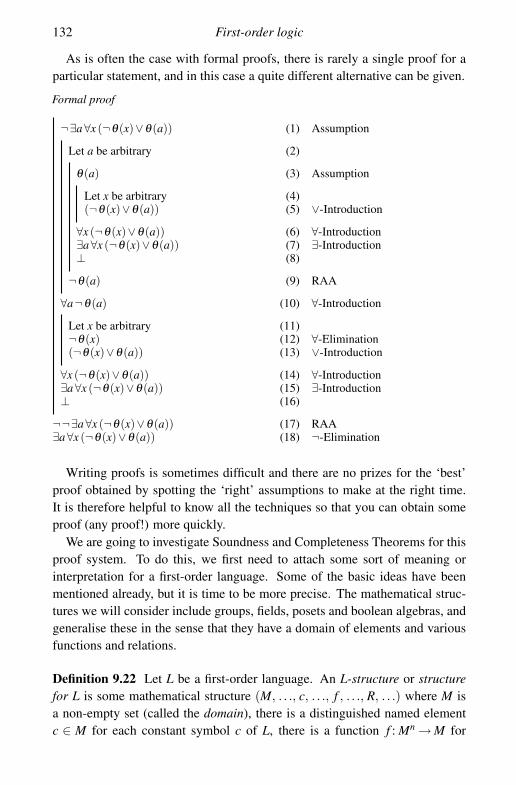
132 First-order logic
As is often the case with formal proofs, there is rarely a single proof for aparticular statement, and in this case a quite different alternative can be given.
Formal proof
¬∃a∀x (¬θ(x)∨θ(a)) (1) Assumption
Let a be arbitrary (2)
θ(a) (3) Assumption
Let x be arbitrary (4)(¬θ(x)∨θ(a)) (5) ∨-Introduction
∀x (¬θ(x)∨θ(a)) (6) ∀-Introduction∃a∀x (¬θ(x)∨θ(a)) (7) ∃-Introduction⊥ (8)
¬θ(a) (9) RAA
∀a¬θ(a) (10) ∀-Introduction
Let x be arbitrary (11)¬θ(x) (12) ∀-Elimination(¬θ(x)∨θ(a)) (13) ∨-Introduction
∀x (¬θ(x)∨θ(a)) (14) ∀-Introduction∃a∀x (¬θ(x)∨θ(a)) (15) ∃-Introduction⊥ (16)
¬¬∃a∀x (¬θ(x)∨θ(a)) (17) RAA∃a∀x (¬θ(x)∨θ(a)) (18) ¬-Elimination
Writing proofs is sometimes difficult and there are no prizes for the ‘best’proof obtained by spotting the ‘right’ assumptions to make at the right time.It is therefore helpful to know all the techniques so that you can obtain someproof (any proof!) more quickly.
We are going to investigate Soundness and Completeness Theorems for thisproof system. To do this, we first need to attach some sort of meaning orinterpretation for a first-order language. Some of the basic ideas have beenmentioned already, but it is time to be more precise. The mathematical struc-tures we will consider include groups, fields, posets and boolean algebras, andgeneralise these in the sense that they have a domain of elements and variousfunctions and relations.
Definition 9.22 Let L be a first-order language. An L-structure or structurefor L is some mathematical structure (M, . . ., c, . . ., f , . . ., R, . . .) where M isa non-empty set (called the domain), there is a distinguished named elementc ∈ M for each constant symbol c of L, there is a function f : Mn → M for

9.1 First-order languages 133
each function symbol f of arity n in L (so, in particular M is closed under thisfunction), and there is a relation R ⊆ Mm for each relation symbol R of L ofarity m.
As is common mathematical practice, we often talk about ‘the structure M’rather than ‘the structure (M, . . ., c, . . ., f , . . ., R, . . .)’ when the operations onM are understood. Note too that our normal notation confuses the distinctionbetween the symbol in L for a function f , constant c or relation R with theactual operation in M that interprets this symbol. Again this is standard math-ematical shorthand, but would not satisfy a pedantic logician. If absolutelynecessary, authors may use a different font or face, or use underlining or someother typographical device, for the symbol, as opposed to its interpretation ina structure.
Example 9.20 shows why we insist that our structures always have non-empty domain. If we allowed empty domains the Soundness Theorem (Theo-rem 9.25 below) would be false.
A sentence of L is one with no free variables, so must be either true or falsein any L-structure. To determine which, we need to interpret the quantifiers∀x . . . and ∃x . . . as ranging over all possible values x of the domain of M. Thisis possibly the most important feature of first-order logic: that all variablesrange over the same set of individuals. This feature distinguishes first-orderlogic from second-order logic (where it is possible to have variables rangingover subsets of the domain) or higher-order logics with sets of sets, and so on.
Definition 9.23 Let L be a first-order language and M an L-structure. If σ isa sentence of L, we write M �σ for ‘σ is true in M’. If Σ is a set of sentenceswe write M �Σ to mean M �σ for all σ ∈ Σ.
If an L-formula φ has free variables, these variables must be given somemeaning or interpretation in an L-structure M before we can say what it meansfor M � φ . In other words, these free variables should be replaced by con-stant symbols or closed terms with specific meaning in M. However, if somemeaning is defined or understood for these variables, and we are arguing in aninformal sense rather than a picky and pedantic way, we can use this under-stood meaning to make sense of M �φ for such formulas φ too.
Structures are used to define the notion Σ � τ , which is essential for thestatement of the Soundness and Completeness Theorems.
Definition 9.24 Let L be a first-order language, Σ a set of L-sentences and τa further L-sentence. Then we write Σ � τ to mean: for all L-structures M, ifM �Σ then M � τ .

134 First-order logic
As before, Σ � τ is vacuously true if there are no L-structures M makingM �Σ true. In this case, Σ� τ for any τ whatsoever.
Theorem 9.25 (Soundness) Let L be a first-order language, Σ a set of L-sentences and τ a further L-sentence. Then Σ� τ implies Σ� τ .
Sketch-proof of Soundness Theorem Formally, the proof is by induction on the(finite) length of the derivation. We simply need to inspect each proof rule tocheck that it preserves the property ‘Σ� τ implies Σ� τ’ for all Σ, τ .
I am not going to prove the Soundness Theorem in any more detail here. A fullproof would involve a more formal definition of what it really means for anL-sentence θ to be true in an L-structure M. This can be done (by induction onthe number of symbols in θ ) but is unenlightening for the beginner and onlybecomes really useful in much more advanced work. Instead, I shall appealto the reader’s common sense and mathematical experience that the rules justgiven look like they should be correct and are in fact particular proof rules thathe/she is accustomed to using anyway.
The Soundness Theorem is really a piece of mathematical book-keeping,checking that our proof rules are reasonable. It is chiefly used in its contra-positive form, Σ �� τ implies Σ � � τ , which gives us a version of a very familiartechnique to show something is not provable, to wit: find counter-example Min which Σ is true but τ is not. Then M shows that Σ �� τ , so Σ � � τ .
9.2 Examples and exercises
In exercises that use the → symbol, use the additional Rules of →-Introductionand Elimination given in Remark 9.11.
Exercise 9.26 Express the following in the first-order language for the realswith non-logical symbols 0, 1, +, ×, −, <.
(i) There is a square-root of 2.(ii) Every non-zero number has a multiplicative inverse.
(iii) Some negative number has a square-root.
Exercise 9.27 Consider the following:
(i) ∀v (θ(v)→ψ(v))(ii) ∀v θ(v)→∀v ψ(v)
(iii) ∃v θ(v)→∃v ψ(v)

9.2 Examples and exercises 135
Prove that (i) implies (ii). Prove as many other implications between thesethree statements as you can.
Exercise 9.28 Let L be the first-order language with a unary function symbol fand constants 0, 1. Prove that from the sentences
∀x ( f (x) = 0∨ f (x) = 1)
and
∃x∃y∃z (¬x = y∧¬y = z∧¬z = x)
you may deduce
∃x∃y (¬x = y∧ f (x) = f (y)).
Exercise 9.29 Let L be the first-order language with a unary function sym-bol f . Prove that from the sentences
∀x ( f ( f (x)) = x),
∀x∀y∀z∀w (x = y∨ x = z∨ x = w∨ y = z∨ y = w∨ z = w),
and
∃x∃y∃z (¬x = y∧¬y = z∧¬z = x)
you may deduce
∃u f (u) = u.
Exercise 9.30 A (simple) graph is usually defined as a non-empty set V ofvertices together with a set E of edges, which are considered as unorderedpairs of vertices. Define a graph as a first-order structure where the domain isthe set of vertices and the edges are represented by a binary relation symbol E,and E(x, y) holds if and only if there is an edge from x to y.
Which first-order axiom(s) is(are) also required for your graphs to corre-spond to the usual ones?
Exercise 9.31 Write down statements in the first-order language of graphs ofExercise 9.30 stating the following.
(i) Between and two vertices there is a path of length at most 4.(ii) There is a cycle of length 4 but no cycle of length 3.
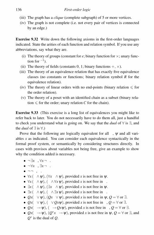
136 First-order logic
(iii) The graph has a clique (complete subgraph) of 5 or more vertices.(iv) The graph is not complete (i.e. not every pair of vertices is connected
by an edge.)
Exercise 9.32 Write down the following axioms in the first-order languagesindicated. State the arities of each function and relation symbol. If you use anyabbreviations, say what they are.
(i) The theory of groups (constant for e; binary function for ×; unary func-tion for −1).
(ii) The theory of fields (constants 0, 1; binary functions +, ×).(iii) The theory of an equivalence relation that has exactly five equivalence
classes (no constants or functions; binary relation symbol R for theequivalence relation).
(iv) The theory of linear orders with no end-points (binary relation � forthe order relation).
(v) The theory of a poset with an identified chain as a subset (binary rela-tion � for the order; unary relation C for the chain).
Exercise 9.33 (This exercise is a long list of equivalences you might like torefer back to later. You do not necessarily have to do them all, just a handfulto check you understand what is going on. We say that the dual of ∀ is ∃, andthe dual of ∃ is ∀.)
Prove that the following are logically equivalent for all φ , ψ and all vari-ables x as indicated. You can consider each equivalence syntactically in theformal proof system, or semantically by considering structures directly. Incases with provisos about variables not being free, give an example to showwhy the condition added is necessary.
• ¬∃x φ , ∀x¬φ .• ¬∀x φ , ∃x¬φ .• ¬¬φ , φ .• ∀x (φ ∧ψ), (∀x φ ∧ψ), provided x is not free in ψ .• ∀x (φ ∧ψ), (φ ∧∀x ψ), provided x is not free in φ .• ∃x (φ ∧ψ), (∃x φ ∧ψ), provided x is not free in ψ .• ∃x (φ ∧ψ), (φ ∧∃x ψ), provided x is not free in φ .• Qx(φ ∨ψ), (Qxφ ∨ψ), provided x is not free in ψ , Q = ∀ or ∃.• Qx(φ ∨ψ), (φ ∨Qxψ), provided x is not free in φ , Q = ∀ or ∃.• Qx(φ →ψ), (φ →Qxψ), provided x is not free in φ , Q = ∀ or ∃.• Qx(φ →ψ), (Q∗xφ →ψ), provided x is not free in ψ , Q = ∀ or ∃, and
Q∗ is the dual of Q.

9.3 Second- and higher-order logic* 137
Exercise 9.34 Use the previous exercise and induction to show that everyformula ψ(x1, . . ., xk) in some first-order language L is equivalent to a formulain prenex normal form, i.e. to a formula in the same language L of the formQ1y1. . .Qlylθ(x1, . . ., xk, y1. . ., yl) where each Qi is ∀ or ∃ and the formulaθ(x1, . . ., xk, y1. . ., yl) contains no quantifiers.
Exercise 9.35 (a) Show that from ∀x∃y∀z ((¬R(x, y)∧S(y, z))∨R(x, z)) youmay prove ∀v∃w∀x ((¬R(v, w)∧S(w, x))∨R(v, x)).
(b) Explain in as general terms as you can how the proof rules for first-orderlogic enable you to rename all bound variables in a sentence σ (providing thereare no name clashes or illegal substitutions, of course).
(c*) Attempt to state and prove a general theorem on renaming variables informulas. (The proof will be by induction on the complexity of formulas.)
Exercise 9.36 Give a modified set of proof rules for first-order logic that allowfor empty domains. Check that the Soundness Theorem holds for your logicand that, on adding the single statement ∃x(x = x) as an axiom, all the provablestatements are exactly those of the normal first-order logic.
9.3 Second- and higher-order logic*
Calling our logic ‘first-order’ begs the question as to what ‘second-order’logic is.
The essential feature of first-order logic is that the quantifiers ∀x . . . and∃x . . . are only allowed to range over elements of a non-empty domain, thedomain of the structure M under consideration. This limits the things one cansay quite considerably. For example it is possible to say that a structure G is agroup in first-order logic, but it is not possible to say that G is a simple group.The obvious attempts fail because the usual definition is that G is a group if andonly if it has no subset N ⊆ G containing the identity and closed under certainoperations (multiplication, inverse, and conjugation by arbitrary elements ofG) other than {1} or G itself. This seems to require a quantifier over subsetsof the structure, and first-order logic does not have this.
The reader should be very wary of any false sense of security in these argu-ments. They are sometimes rather deep and often very difficult. I did not proveanything in the last paragraph – only pointed out that the obvious attempt tosay in first-order logic that ‘G is simple’ fails. At this stage, it seems possiblethat there are other less obvious approaches. In fact, it really cannot be done,but we will not have the apparatus to prove this until the next chapter. (See

138 First-order logic
Exercise 10.17 for a hint.) In contrast, some cases can be done: we can de-scribe all simple groups of order 168 (or any other finite order) by a first-ordersentence, for example.
Second-order logic allows for these subset-quantifiers. A particular lan-guage for second-order logic is obtained from one for first-order logic byadding a new set of variables X j
i for each i, j ∈ N. The idea is that X ji ranges
over subsets of M j, where M is the structure under consideration. We alsoadd new atomic formulas (t1, . . ., t j) ∈ X j
i for every i, j and terms t1, . . ., t j.We allow these new atomic formulas to take part in more complex formulasand build up the notion of a second-order formula in a similar way to that forfirst-order formulas. The structures for a second-order language are the sameas those for the corresponding first-order language.
In fact, although we have added second-order variables X ji of all ‘types’ j,
thinking of X ji as ranging over subsets of M j, we never need more than the
first three cases, j = 1, 2, 3. This is because there is always a bijection from aninfinite set M to its cartesian power M2.
Exercise 9.37 Assume the assertion just made, that for any infinite set Mthere is a bijection f : M →M2. Write down a formula in second-order logicthat expresses the fact that X3
1 is the set {(x, y, z) : z = f (x, y)} for some suchfunction f . Use this to show that second-order variables of ‘type’ greater thanthree are unnecessary.
This then gives the main ideas of second-order logic. We have a language, agrammar explaining how formulas are built, and a notion of what it means fora second-order sentence to be true in a structure M. (For the latter all we needto know is that M �∃X j
i θ(X ji ) holds if and only if M �θ(A) for some A ⊆ M j
and M �∀X ji θ(X j
i ) holds if and only if M � θ(A) for all A ⊆ M j, and use theother ideas from first-order logic.)
If this seems interesting, then good: it is interesting – in fact, far too in-teresting! Some structures, such as those for the reals and the naturals, canbe characterised completely by the second-order sentences true in them, andsentences achieving this were first written down by Dedekind and, in the caseof the naturals, independently by Peano. The real problem comes when onetries to put right the most conspicuous omission in the account of second-orderlogic: the lack of any system for proof. There is no such system, and in fact it isa consequence of Godel’s famous theorem on the incompleteness of arithmeticthat there cannot be such a second-order system for N that is any better thansimply writing down all the true sentences and using them as a set of axioms.(This is not what we want: we want a way of discovering new true statements!)

9.3 Second- and higher-order logic* 139
There are possible ways round at least some of the problems here. One is tochange our idea of structure to allow two or more domains: one of numbers orobjects, and another of sets of objects, for example. Thus the structure for thenatural numbers becomes (N, P(N), P(N2), P(N3), . . ., 0, 1, . . .), where P(S)is the power-set or set of all subsets of S. We can even write down somesuitable axioms, such as the axiom of extensionality saying two sets are equalif and only if their elements (in the sense of the symbol ∈) are the same, andalso lists of axioms – called axiom schemes – expressing the existence of plentyof sets, such as
∃X11 ∀x (x ∈ X1
1 ↔θ(x))
for all second-order formulas θ(x). (This particular axiom scheme is calledcomprehension.)
As a tool for proving statements about the naturals, the approach just sug-gested is quite powerful. But in fact, it is just first-order logic in disguise onceagain. Consider structures of the form
(N∪P(N)∪P(N×N)∪ . . ., N, S1, S2, S3, . . ., ∈1, ∈2, ∈3, . . ., 0, 1, . . .)
where N, S1, S2, S3 are all unary relations: N(x) means ‘x is a number’ orx ∈ N; S1(x) means ‘x is a set’ or x ⊆ N; S2(x) means ‘x is a set of pairs’ orx ⊆ N×N; and S3(x) means ‘x is a set of triples’; etc. The k + 1-ary relation(x1, . . ., xk) ∈k s means ‘the k-tuple (x1, . . ., xk) is a member of the set s.’.
A similar approach can be used for even stronger third-order logic wherevariables ranging over sets of sets are introduced, or for higher-order logic.An even more powerful approach is to adopt a first-order set theory such asZermelo–Frankel as a base theory to prove statements about N. This behavesrather like nth order logic for all n, including transfinite n, and amazingly is afirst-order theory in the language with a single binary relation symbol, ∈. Thuswe return, very squarely, back to the realm of first-order logic.

10
Completeness and compactness
10.1 Proof of completeness and compactness
This chapter is devoted to the main theorem for first-order logic, the Complete-ness Theorem.
Theorem 10.1 (Completeness) Let L be a first-order language, Σ a set ofL-sentences and τ a further L-sentence. Then Σ� τ implies Σ� τ .
By contrast with the Soundness Theorem, the Completeness Theorem forfirst-order logic is a powerful mathematical tool with very many interestingconsequences and applications. Its proof involves an application of Zorn’sLemma in an essential way, and will take us quite a bit longer. We startby looking at a way of adding new constant symbols to the language, called‘Henkinisation’, and named after the logician Leon Henkin who first used thismethod.
Definition 10.2 Let L be a first-order language. We consider for each formulaφ(x) with a single free variable x a new constant symbol ε . (‘New’ here meansthat these constants are distinct symbols not already in L. We only need asupply of new symbols and we may assume that there are always enough newsymbols available.) Since there will be one such constant ε for each φ(x)and we require these symbols to be all distinct we shall denote the symbolcorresponding to φ(x) by εφ(x). This is just a name for a new symbol whichis used to indicate this symbol’s use in the formulas below. There is no newlogical rule being introduced here.
The first Henkinisation of L is the first-order language H(L) consisting of Ltogether with all εφ(x).
The second Henkinisation of L is the first-order language H(H(L)) consist-
140
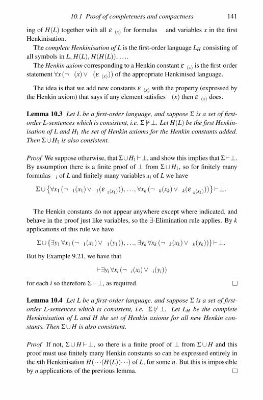
10.1 Proof of completeness and compactness 141
ing of H(L) together with all εφ(x) for formulas φ and variables x in the firstHenkinisation.
The complete Henkinisation of L is the first-order language LH consisting ofall symbols in L, H(L), H(H(L)), . . ..
The Henkin axiom corresponding to a Henkin constant εφ(x) is the first-orderstatement ∀x (¬φ(x)∨φ(εφ(x))) of the appropriate Henkinised language.
The idea is that we add new constants εφ(x) with the property (expressed bythe Henkin axiom) that says if any element satisfies φ(x) then εφ(x) does.
Lemma 10.3 Let L be a first-order language, and suppose Σ is a set of first-order L-sentences which is consistent, i.e. Σ � �⊥. Let H(L) be the first Henkin-isation of L and H1 the set of Henkin axioms for the Henkin constants added.Then Σ∪H1 is also consistent.
Proof We suppose otherwise, that Σ∪H1�⊥, and show this implies that Σ�⊥.By assumption there is a finite proof of ⊥ from Σ∪H1, so for finitely manyformulas φi of L and finitely many variables xi of L we have
Σ∪{∀x1 (¬φ1(x1)∨φ1(εφ1(x1))), . . ., ∀xk (¬φk(xk)∨φk(εφk(xk)))}�⊥.
The Henkin constants do not appear anywhere except where indicated, andbehave in the proof just like variables, so the ∃-Elimination rule applies. By kapplications of this rule we have
Σ∪{∃y1 ∀x1 (¬φ1(x1)∨φ1(y1)), . . ., ∃yk ∀xk (¬φk(xk)∨φk(yk))}�⊥.
But by Example 9.21, we have that
�∃yi ∀xi (¬φi(xi)∨φi(yi))
for each i so therefore Σ�⊥, as required.
Lemma 10.4 Let L be a first-order language, and suppose Σ is a set of first-order L-sentences which is consistent, i.e. Σ � � ⊥. Let LH be the completeHenkinisation of L and H the set of Henkin axioms for all new Henkin con-stants. Then Σ∪H is also consistent.
Proof If not, Σ∪H �⊥, so there is a finite proof of ⊥ from Σ∪H and thisproof must use finitely many Henkin constants so can be expressed entirely inthe nth Henkinisation H(· · ·(H(L))· · ·) of L, for some n. But this is impossibleby n applications of the previous lemma.

142 Completeness and compactness
Lemma 10.5 Let L be a first-order language, and suppose Σ is a consistentset of first-order L-sentences, and θ is a further L-sentence. Then at least oneof Σ∪{θ}, Σ∪{¬θ} is also consistent.
Proof If Σ∪{θ}�⊥ then by Reductio Ad Absurdum Σ�¬θ . But then wecannot have Σ∪{¬θ}�⊥, for this would mean that Σ�⊥. So either Σ∪{θ} ��⊥ or Σ∪{¬θ} ��⊥.
We are now in a position to prove the Completeness Theorem.We shall suppose that Σ � � τ and find a structure M making Σ true but not τ .
It will follow that Σ �� τ , thus proving the contrapositive of the CompletenessTheorem.
By a now familiar application of the Reductio Ad Absurdum Rule, Σ � � τimplies Σ∪ {¬τ} is consistent. If we can show that there is a structure Mmaking Σ∪{¬τ} true it would follow that M � Σ and M �� τ hence Σ �� τ , asrequired.
Let LH be the complete Henkinisation of L, and H the set of Henkin axioms.By the lemma on Henkinisation, Σ0 = Σ∪H ∪{¬τ} is consistent. We lookat the set X of all consistent sets of LH sentences Ξ ⊇ Σ0, and order X by ⊆.This makes X into a poset with the Zorn property since any chain Y ⊆ X hasupper bound Ξ =
⋃Y = {σ : σ ∈ Γ, for some Γ ∈ Y}. (The argument that this
is consistent has been given before and simply requires that proofs are finiteobjects and Y is a chain.) Therefore there is a set Σ+ ∈ X which is consistent,contains Σ0, and is maximal. By maximality and the previous lemma, Σ+ ∈ Xhas the property that for all sentences θ of LH we have either θ ∈ Σ+ or ¬θ ∈Σ+.
The set Σ+ contains all the information we need. Notice that if σ is any LH -sentence and Σ+ �σ then σ ∈ Σ+. The process from now on requires definingour L-structure M and checking various properties such as well-definedness,and that the structure we define satisfies the sentences in Σ0. Each step in theprocess uses the maximality of Σ+ and will also require applications of theindividual proof rules for our system.
First, we need to define M. The domain of M is defined to be the set T of allclosed terms of LH , factored out by the equivalence relation
t ∼ s if and only if t = s ∈ Σ+.
Clearly the first task is to show this is an equivalence relation. This uses theequality rules of first-order logic. If t ∈ T then �t = t, so t = t ∈ Σ+ hence t ∼ tand ∼ is reflexive. If t, s ∈ T and t ∼ s then t = s ∈ Σ+ so Σ+� s = t and hence

10.1 Proof of completeness and compactness 143
s ∼ t. Also if t, s, r ∈ T and t ∼ s and s ∼ r then t = s, s = r ∈ Σ+ so Σ+� t = rhence t ∼ r. Thus ∼ is an equivalence.
Write [t] for the equivalence class of t ∈ T . We must next define the con-stants, relations and functions on M. This is done as follows:
• for each constant symbol c, the corresponding element of M is [c];• for each n-ary relation symbol R, we define the meaning of R on M by
R([t1], . . ., [tn]) if and only if R(t1, . . ., tn) ∈ Σ+;• for each n-ary function symbol f , we define the meaning of f in M by
f ([t1], . . ., [tn]) = [ f (t1, . . ., tn)].
Our next task is to show that the functions and relations here are well definedand do not depend on the choice of representatives t1, . . ., tn of [t1], . . ., [tn].There is nothing to do for the constant symbols. For a relation symbol R wemust prove that if R(t1, . . ., tn) ∈ Σ+ and si ∼ ti for each i then R(s1, . . ., sn) ∈Σ+. But this follows from maximality: R(t1, . . ., tn) ∈ Σ+ and si = ti ∈ Σ+ foreach i implies that Σ+ �R(s1, . . ., sn) by the Substitution Rule. The treatmentof function symbols is similar; here we must prove that if si ∼ ti for each ithen f (t1, . . ., tn) ∼ f (s1, . . ., sn). Applying the Substitution Rule to the for-mula θ(x1, . . ., xn) defined to be f (t1, . . ., tn) = f (x1, . . ., xn) we have Σ+ �θ(t1, . . ., tn), by the Reflexivity Rule, hence Σ+ � f (t1, . . ., tn) = f (s1, . . ., sn)by substitution.
Finally we have to show that M makes Σ0 true. In fact, as in the proof ofthe Completeness Theorem for propositional logic, it is easier to show thatM makes Σ+ true, and we do this by an induction on the ‘size’ of a sentenceθ . For the purposes of this proof, we say a connective is one of the symbols¬ , ∨ , ∧ , ∀, ∃. Then we show inductively that
• for all θ with at most n connectives we have: M � θ if and only if θ ∈Σ+.
If θ has 0 connectives, it may be t = s for some t, s ∈ T . Observe that itis quite possible for two different closed terms t, s ∈ T to represent the sameobject in M. But by the definition of M, M � t = s holds if and only if t ∼ swhich, by the definition of ∼, holds if and only if t = s ∈ Σ+.
The other possibility when θ has 0 connectives is when θ is R(t1, . . ., tn),for some relation symbol R and some terms ti. But then, by the definition of Rin M, M �R(t1, . . ., tn) if and only if R(t1, . . ., tn) ∈ Σ+.
We now suppose θ has one or more connectives and use our induction hy-pothesis on formulas with fewer connectives.
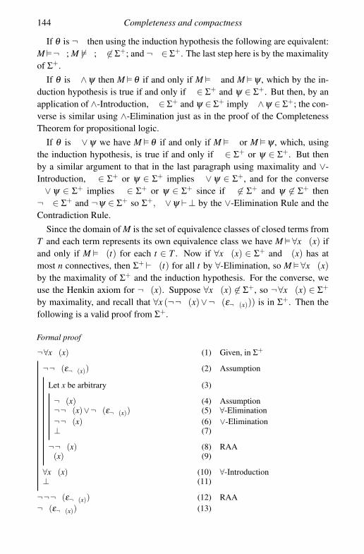
144 Completeness and compactness
If θ is ¬φ then using the induction hypothesis the following are equivalent:M �¬φ ; M ��φ ; φ �∈ Σ+; and ¬φ ∈ Σ+. The last step here is by the maximalityof Σ+.
If θ is φ ∧ψ then M � θ if and only if M � φ and M � ψ , which by the in-duction hypothesis is true if and only if φ ∈ Σ+ and ψ ∈ Σ+. But then, by anapplication of ∧-Introduction, φ ∈ Σ+ and ψ ∈ Σ+ imply φ ∧ψ ∈ Σ+; the con-verse is similar using ∧-Elimination just as in the proof of the CompletenessTheorem for propositional logic.
If θ is φ ∨ψ we have M � θ if and only if M � φ or M � ψ , which, usingthe induction hypothesis, is true if and only if φ ∈ Σ+ or ψ ∈ Σ+. But thenby a similar argument to that in the last paragraph using maximality and ∨-Introduction, φ ∈ Σ+ or ψ ∈ Σ+ implies φ ∨ψ ∈ Σ+, and for the converseφ ∨ ψ ∈ Σ+ implies φ ∈ Σ+ or ψ ∈ Σ+ since if φ �∈ Σ+ and ψ �∈ Σ+ then¬φ ∈ Σ+ and ¬ψ ∈ Σ+ so Σ+, φ ∨ψ �⊥ by the ∨-Elimination Rule and theContradiction Rule.
Since the domain of M is the set of equivalence classes of closed terms fromT and each term represents its own equivalence class we have M �∀x φ(x) ifand only if M � φ(t) for each t ∈ T . Now if ∀x φ(x) ∈ Σ+ and φ(x) has atmost n connectives, then Σ+ �φ(t) for all t by ∀-Elimination, so M �∀x φ(x)by the maximality of Σ+ and the induction hypothesis. For the converse, weuse the Henkin axiom for ¬φ(x). Suppose ∀x φ(x) �∈ Σ+, so ¬∀x φ(x) ∈ Σ+
by maximality, and recall that ∀x (¬¬φ(x)∨¬φ(ε¬φ(x))) is in Σ+. Then thefollowing is a valid proof from Σ+.
Formal proof
¬∀x φ(x) (1) Given, in Σ+
¬¬φ(ε¬φ(x)) (2) Assumption
Let x be arbitrary (3)
¬φ(x) (4) Assumption¬¬φ(x)∨¬φ(ε¬φ(x)) (5) ∀-Elimination¬¬φ(x) (6) ∨-Elimination⊥ (7)
¬¬φ(x) (8) RAAφ(x) (9)
∀x φ(x) (10) ∀-Introduction⊥ (11)
¬¬¬φ(ε¬φ(x)) (12) RAA¬φ(ε¬φ(x)) (13)

10.1 Proof of completeness and compactness 145
This shows that ε¬φ(x) is a t ∈ T such that φ(t) �∈ Σ+, so M �� φ(t) by theinduction hypothesis. Hence M ��∀x φ(x), as required.
The case of the ∃ quantifier is similar. For one direction, if M � ∃x φ(x)where φ(x) has at most n connectives then M �φ(t) for some t ∈ T , so φ(t) ∈Σ+ by the induction hypothesis, and hence ∃x φ(x) ∈ Σ+ by maximality ofΣ+ and ∃-Introduction. Conversely, if ∃x φ(x) ∈ Σ+ then since we also have∀x (¬φ(x)∨φ(εφ(x))) ∈ Σ+ the following is a proof from Σ+.
Formal proof
∃x φ(x) (1) Given, in Σ+
Let a satisfy φ(a) (2)¬φ(a)∨φ(εφ(x)) (3) ∀-Elimination
¬φ(a) (4) Assumption⊥ (5)
¬¬φ(a) (6) RAAφ(εφ(x)) (7) ∨-Elimination
φ(εφ(x)) (8) ∃-Elimination
So the term t = εφ(x) has φ(t) in Σ+ hence M � φ(t) by induction, and soM �∃x φ(x), as required.
This completes the inductive proof that M � Σ+ and hence completes theproof of the Completeness Theorem.
The Completeness and Soundness Theorems are interesting from a founda-tional point of view (where they show that just about any mathematical proofcan be expressed in a formal system which is mechanically checkable), but arealso powerful mathematical tools in their own right. We will be investigatingthem as mathematics in the next two chapters, but we can give here a samplecorollary, the Compactness Theorem. It is a powerful result allowing us toconstruct new mathematical structures, and is proved by using the Soundnessand Completeness Theorems together to allow us to pass between the worldsof proofs and mathematical structures.
Theorem 10.6 (Compactness) Let L be a first-order language and Σ a setof L-sentences. Suppose that each finite subset Γ of Σ has a structure MΓ � Γmaking Γ true. Then there is a structure M making the whole of Σ true.
Proof By assumption and the Soundness Theorem, each finite Γ ⊆ Σ is consis-tent, Γ � �⊥. This means Σ is consistent too, since a proof of ⊥ from Σ is finiteso can only use finitely many assumptions from Σ. So Σ � �⊥. It follows from

146 Completeness and compactness
the Completeness Theorem that there is a structure M making the whole of Σtrue.
10.2 Examples and exercises
For the next few paragraphs and exercises, we shall examine the ‘pure’ first-order language L0 with = and all the other logical symbols, but no non-logicalsymbols.
Exercise 10.7 Indicate how to write down sentences σn and τn of L0 with thefollowing meanings.
• σn: There are at least n elements in the domain.• τn: There are exactly n elements in the domain.
(Hint: use plenty of variables. Look at Exercises 9.28 and 9.29 for ideas.)
Exercise 10.8 Write out a formal proof showing that σ3 �σ2.
Exercise 10.9 Explain why a structure M satisfies
S∞ = {σn : n ∈ N}if and only if its domain is infinite.
The last exercise shows that the class of infinite M is axiomatisable in L0,i.e. there is a set of sentences of L0 such that M is infinite if and only if itsatisfies all these sentences.
Example 10.10 The class of infinite M is not finitely axiomatisable in thelanguage L0, i.e. there is no single sentence σ∞ of L0 which is satisfied in astructure M if and only if the domain of M is infinite.
Proof If σ∞ is such a sentence it must be that σ∞ �σk for all k. This is bythe Completeness Theorem, because clearly σ∞ � σk for all k. Similarly, bycompleteness, there is a proof p of σ∞ from the set of sentences S∞, since onceagain S∞ � σ∞. But proofs are finite objects, so there is a finite subset of S∞such that
σ1, . . ., σn �σ∞ �σk
for all k. In particular this would imply that
σ1, . . ., σn �σn+1.

10.2 Examples and exercises 147
But this is impossible since there is an L0 structure with exactly n elements,and this satisfies σ1, . . ., σn but not σn+1, so
σ1, . . ., σn ��σn+1
hence
σ1, . . ., σn � �σn+1
by the Soundness Theorem.
Exercise 10.11 Show that there is no set S f of L0-sentences such that a struc-ture satisfies S f if and only if its domain is finite. (Hint: if such a set S f exists,show that S f ∪{σ1, . . ., σn} is consistent for all n. Using compactness or oth-erwise, derive a contradiction.)
Exercise 10.12 Find a single sentence θ in a (necessarily different) first-orderlanguage L that only has infinite models.
Exercise 10.13 Show that the following properties of a graph (representedin a first-order language as in Exercise 9.30) are not equivalent to any set offirst-order statements in this language.
(i) The graph is connected, i.e. between any two vertices there is a finitepath connecting them.
(ii) The graph is not a forest, i.e. it has a finite cycle.(iii) There is no infinite clique in the graph.
Example 10.14 The first-order theory of groups can be described in the lan-guage LG with one constant symbol e for the identity, one binary functionsymbol × for the group multiplication and one unary function −1 for inverses.The theory of groups is the set of LG sentences
• ∀x∀y∀z ((x× y)× z = x× (y× z))• ∀x (x× e = x∧ e× x = x)• ∀x (x× x−1 = e∧ x−1 × x = e)
so that a group is an LG structure satisfying these sentences. (Note that ‘clo-sure under multiplication and inverses’ is automatic from our definition of LG-structure.)
Example 10.15 A cyclic group is a group G generated by a single element x,that is G = {xn : n ∈ Z} where x0 = e and x−n = (x−1)n for negative exponents.

148 Completeness and compactness
Then, in contrast with the last example, the set of cyclic groups is not axioma-tisable, i.e. there is no set of first-order sentences true for precisely the cyclicgroups.
Proof Define a set of first-order sentences involving two new constant symbolsa, b and the other LG operations by
Γ ={¬an = bk : n, k ∈ Z, not both zero
}.
Here, an abbreviates some term in the language involving a, × and possiblyalso e (if n = 0) and −1 (if n < 0). Then if G is a group and a, b ∈ G�Γ then Gis not cyclic, for if G is generated by x ∈ G we have a = xr and b = xs for somer, s ∈ Z and so as = xrs = br so r = s = 0 by Γ. But this would mean a = b = eso an = bk for all n, k, contradicting Γ.
Now suppose Σ is a set of sentences containing the axioms for group theoryand such that each σ ∈ Σ is true in all cyclic groups. To show that Σ does notaxiomatise all cyclic groups it suffices to find a non-cyclic group satisfying Σ.To this end, let N0 ∈ N and let
Γ0 ={¬an = bk : n, k ∈ Z, not both zero, |n|, |k| < N0
}.
Now consider
C ={. . ., x−2, x−1, x0, x1, x2, . . .
},
the infinite cyclic group generated by x. Then C � Σ as C is cyclic. Let a = xand b = xN0 . Then if an = bk with |n|, |k| < N0 we have kN0 −n = 0 which hasn = k = 0 as its only solution. Thus C �Γ0.
The previous paragraph shows that for each finite subset Γ0 ⊆ Γ there is agroup C with a, b ∈ C such that (C, a, b)� Γ0 ∪Σ. By the Compactness The-orem it follows that there is a group G with elements a, b ∈ G and (G, a, b)�Γ ∪ Σ. So this group satisfies Σ but is not cyclic as it also satisfies Γ, asrequired.
The technique of going to an expanded language by adding constants and thenapplying the Compactness Theorem is typical, and we will see other exampleslike this.
Exercise 10.16 Which of the following classes of groups is axiomatisable inthe language LG of Example 10.14? Finitely axiomatisable in LG? Give proofs.
(i) The class of groups of size n (for some fixed n ∈ N).(ii) The class of all groups of size at most n (for some fixed n ∈ N).
(iii) The class of all infinite groups.

10.3 The Compactness Theorem and topology* 149
(iv) The class of all finite groups.(v) The class of all torsion groups.
(vi) The class of all n-torsion groups.(vii) The class of all torsion-free groups.
(A group G is n-torsion if gn = e for all g ∈ G. It is torsion if for all g ∈ Gthere is n ∈ N such that gn = e, and it is torsion-free if for all g ∈ G, if g �= ethen gn �= e for all n ∈ N.)
There are very many ways of doing the next exercise, and it is instructive totry several and see what extra information each gives. Possibly the simplest isto note that an abelian group is simple if and only if it is cyclic of prime order.By compactness every set of sentences true in all simple abelian groups is alsotrue in some infinite group.
Exercise 10.17 Prove that the class of all simple groups is not axiomatisable.
10.3 The Compactness Theorem and topology*
The Compactness Theorem is not idly named. It is actually equivalent to theassertion that a particular topological space is compact. This short optionalsection defines the topological space and shows the connection, and is providedhere for readers with some background knowledge in general topology.
First, we fix a first-order language L. We are interested in L-structures andthe L-sentences that they satisfy.
Definition 10.18 Let M be an L-structure. The theory of M, written ThM, isthe set {σ : M �σ} of all L-sentences true in M.
We can see quickly that the set Σ = ThM has the property
• if σ is any L-sentence then exactly one of σ ∈ Σ or ¬σ ∈ Σ.
This is just a restatement of the fact that every σ is either true or false in astructure for L, but not both.
In fact, by the Soundness Theorem, we can also see that ThM is consistent,i.e. ThM � � ⊥, and the above property shows that it is maximally consistent,i.e. that there is no proper extension which is a set of L-sentences and consis-tent. Also, by the Completeness Theorem, any such maximally consistent setof L-sentences is ThM for some L-structure M. Thus the idea of the theoryof M characterises such maximally consistent sets, though we will not requirethese observations here.
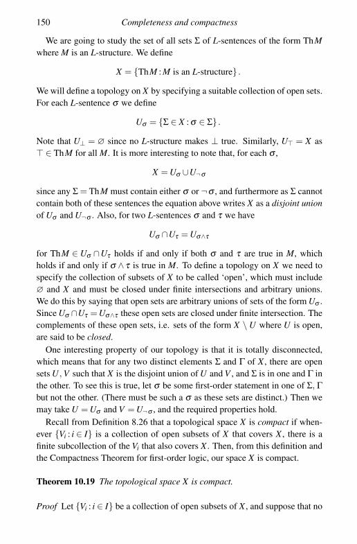
150 Completeness and compactness
We are going to study the set of all sets Σ of L-sentences of the form ThMwhere M is an L-structure. We define
X = {ThM : M is an L-structure} .
We will define a topology on X by specifying a suitable collection of open sets.For each L-sentence σ we define
Uσ = {Σ ∈ X : σ ∈ Σ} .
Note that U⊥ = ∅ since no L-structure makes ⊥ true. Similarly, U� = X as� ∈ ThM for all M. It is more interesting to note that, for each σ ,
X = Uσ ∪U¬σ
since any Σ = ThM must contain either σ or ¬σ , and furthermore as Σ cannotcontain both of these sentences the equation above writes X as a disjoint unionof Uσ and U¬σ . Also, for two L-sentences σ and τ we have
Uσ ∩Uτ = Uσ∧τ
for ThM ∈ Uσ ∩Uτ holds if and only if both σ and τ are true in M, whichholds if and only if σ ∧ τ is true in M. To define a topology on X we need tospecify the collection of subsets of X to be called ‘open’, which must include∅ and X and must be closed under finite intersections and arbitrary unions.We do this by saying that open sets are arbitrary unions of sets of the form Uσ .Since Uσ ∩Uτ = Uσ∧τ these open sets are closed under finite intersection. Thecomplements of these open sets, i.e. sets of the form X \ U where U is open,are said to be closed.
One interesting property of our topology is that it is totally disconnected,which means that for any two distinct elements Σ and Γ of X , there are opensets U , V such that X is the disjoint union of U and V , and Σ is in one and Γ inthe other. To see this is true, let σ be some first-order statement in one of Σ, Γbut not the other. (There must be such a σ as these sets are distinct.) Then wemay take U = Uσ and V = U¬σ , and the required properties hold.
Recall from Definition 8.26 that a topological space X is compact if when-ever {Vi : i ∈ I} is a collection of open subsets of X that covers X , there is afinite subcollection of the Vi that also covers X . Then, from this definition andthe Compactness Theorem for first-order logic, our space X is compact.
Theorem 10.19 The topological space X is compact.
Proof Let {Vi : i ∈ I} be a collection of open subsets of X , and suppose that no

10.3 The Compactness Theorem and topology* 151
finite collection of the Vi covers X . We must show that there is Γ ∈ X which isin none of the Vi.
We first reduce to the case when each Vi is of the form Uσ for some L-sentence σ . Since Vi is open and therefore the union of sets of the form Uσ ,every element in Vi is contained in some Uσ . We now consider the collection ofopen sets {Uσ :Uσ ⊆Vi for some i ∈ I} and note that it covers the same subsetof X as {Vi : i ∈ I}, and also has the property that no finite subcollection of itcan cover the whole of X . It suffices therefore to find Γ ∈ X which is in noneof the Uσ .
To this end, let
Γ = {¬σ :Uσ ⊆Vi for some i ∈ I} .
We claim that there is an L-structure MΓ in which all sentences in Γ hold. Ifnot then, by the Compactness Theorem, there is a finite subset of Γ with nostructure making it true:
{¬σ1, ¬σ2, . . ., ¬σn}�⊥.
This means that no structure M satisfies all of ¬σ1, ¬σ2, . . ., ¬σn and henceno Σ ∈ X can contain all of ¬σ1, ¬σ2, . . ., ¬σn. Thus
Uσ1 ∪Uσ2 ∪ . . .∪Uσn = X
since every structure makes one of σ1, . . ., σn true. But this contradicts theassumption that no finite subcollection of the Uσ covers X . Hence there is astructure MΓ in which Γ is true. Let Γ+ = ThMΓ ∈ X . It is now easy to seethat Γ+ is not an element of any of the Uσ used in the definition of Γ, since¬σ ∈ Γ ⊆ Γ+. This shows that the original collection of open sets Uσ does notcover X , as required.
The reader may be interested to note that this argument only used the Com-pactness Theorem and the idea of an L-structure. Neither Soundness nor Com-pleteness was needed at all. There is a converse argument too: the compactnessof the space X implies the Compactness Theorem as previously given, since ifΓ is a an infinite set of L-sentences with no structure satisfying all σ ∈ Γ then
{U¬σ : σ ∈ Γ}is an open cover of X since every M satisfies some ¬σ . Therefore there is afinite subcover
{U¬σi : i = 1, 2, . . ., n}and hence there is no L-structure satisfying all sentences in {σ1, σ2, . . ., σn}.

152 Completeness and compactness
Exercise 10.20 Express the Compactness Theorem for propositional logic asthe compactness of a suitable topological space X . (For this, see also Proposi-tion 8.35.)
10.4 The Omitting Types Theorem*
The Henkin method used in the proof of the Completeness Theorem is surpris-ingly powerful, and by inspecting it carefully we can get plenty of extra usefulinformation, especially when the language is countable. Model theorists knowthis kind of argument as ‘Omitting Types’ for reasons that will become appar-ent, but from the point of view of topology (as discussed in Section 10.3) it isvery close to the Baire Theorem for compact Hausdorff spaces.
The Omitting Types Theorem is an important and useful result in model the-ory, and many more advanced texts on model theory rightly give it a thoroughpresentation and a long discussion of its applications, how the proof works, andhow the proof may be varied to give related results. Here I shall present onlythe very shortest of proofs for readers comfortable with the topological termi-nology used before. Throughout this section we work with first-order logic incountable languages.
We start by taking a countable first-order language L and a consistent setΣ0 of L-sentences. We add a countably infinite set of constants, W (so thecardinality of W is the same as the cardinality of L) and denote by LW theexpanded language with these constant symbols added. We note the key factthat LW is also a countable first-order language.
Now consider sets of LW -sentences Σ that are deductively closed, i.e. forwhich
Σ�σ implies σ ∈ Σ
for each sentence σ of LW . The set of all such Σ is called the set of LW -theoriesextending Σ0 and will be denoted here by T . Thus
T = {Σ ⊆ LW : Σ is consistent, deductively closed and Σ ⊇ Σ0} .
As in Section 10.3, we make T into a topological space by defining Uσ ={Σ ∈ T : σ ∈ Σ} and saying that open sets are unions of sets of the form Uσ .
If X is a topological space, i.e. a set with specified open subsets, and Y ⊆ Xis a subset of X , then we can regard Y as a topological space with topologyinherited from X by saying that a set U ⊆ Y is open if and only if U = Y ∩Vfor some open V ⊆ X . This topology on Y is called the subspace topology.
Exercise 10.21 In the case when Σ0 = ∅, we can recover our space X of
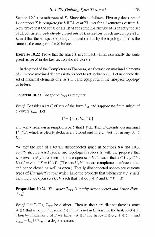
10.4 The Omitting Types Theorem* 153
Section 10.3 as a subspace of T . Show this as follows. First say that a set ofL-sentences Σ is complete for L if Σ�σ or Σ�¬σ for all sentences σ from L.Now prove that the set X of all ThM for some L-structure M is exactly the setof all consistent, deductively closed sets of L-sentences which are complete forL, and that the subspace topology induced on this by the topology on T is thesame as the one given for X before.
Exercise 10.22 Prove that the space T is compact. (Hint: essentially the sameproof as for X in the last section should work.)
In the proof of the Completeness Theorem, we focused on maximal elementsof T , where maximal denotes with respect to set inclusion ⊆. Let us denote theset of maximal elements of T as Tmax, and equip it with the subspace topologyas before.
Theorem 10.23 The space Tmax is compact.
Proof Consider a set C of sets of the form Uσ and suppose no finite subset ofC covers Tmax. Let
Γ = {¬σ :Uσ ∈C}
and verify from our assumptions on C that Γ � �⊥. Then Γ extends to a maximalΓ′ ⊇ Γ, which is clearly deductively closed and in Tmax but not in any Uσ ∈U .
We met the idea of a totally disconnected space in Sections 8.4 and 10.3.Totally disconnected spaces are topological spaces X with the property thatwhenever x �= y in X then there are open sets U , V such that x ∈ U , y ∈ V ,U ∩V = ∅ and X = U ∪V . (The sets U , V here are complements of each otherand hence closed as well as open.) Totally disconnected spaces are extremetypes of Hausdorff spaces which have the property that whenever x �= y in Xthen there are open sets U , V such that x ∈U , y ∈V and U ∩V = ∅.
Proposition 10.24 The space Tmax is totally disconnected and hence Haus-dorff.
Proof Let Σ, Γ ∈ Tmax be distinct. Then as these are distinct there is someσ ∈ Σ that is not in Γ or some τ ∈ Γ that is not in Σ. Assume the first, so σ �∈ Γ.Then by maximality of Γ we have ¬σ ∈ Γ and hence Σ ∈ Uσ , Γ ∈ U¬σ andTmax = Uσ ∪U¬σ is a disjoint union.

154 Completeness and compactness
In a small number of very special cases in certain languages L and base sets Σ0
we can build an L-structure M�Σ+ directly from the set Σ+ ∈ Tmax, often usingan argument similar to the proof of the Completeness Theorem. Unfortunately,these arguments do not work in all cases and in general it requires the Henkinaxioms to work. So we next abstract from the Henkin axioms those propertiesof a set Σ+ ∈ Tmax that are required for the construction in the CompletenessTheorem to work.
Definition 10.25 Say that a set of LW -sentences Σ has the Henkin propertyif whenever φ(x) is an LW -formula in a single free variable then there is aconstant c ∈W such that the sentence
∀x (¬φ(x)∨φ(c))
is Σ.
The Henkin property appears to be a rather technical property of a set ofsentences in LW . We are really interested in LW -structures. The followinglemma indicates the connection.
Lemma 10.26 Suppose Σ+ ∈ Tmax has the Henkin property. Then there isM �Σ+ such that for all elements a ∈ M there is some constant symbol w ∈Wsuch that a realises w.
Proof This is identical to the proof of the Completeness Theorem. We letM = W/∼ where u ∼ v if and only if u = v ∈ Σ+ and M � R([u1], . . ., [uk]) ifand only if R(u1, . . ., uk) ∈ Σ+ for a k-ary relation symbol R, and similarly forfunctions. Then M is well defined and by an induction on formulas using themaximality of Σ+ and the Henkin property we get that M �Σ+.
So, not only do sets of sentences with the Henkin property have structures, butthese structures can be chosen to consist entirely of constants from W .
By Lemma 10.4 and a Zorn’s Lemma argument, maximal sets Σ+ ∈ T withthe Henkin property exist, at least when we choose the constants W to be theHenkin constants in Lemma 10.4. But by renaming these constants, we see thatmaximal sets Σ+ ∈ T with the Henkin property exist whatever W is, provided ithas the same cardinality as L. With the topological setting here we can reviewthis argument and understand it in a more useful form.
First we need some more definitions and a result from topology.
Definition 10.27 Let X be a topological space and A ⊆ X . Then A is co-rareif whenever U ⊆ X is open and non-empty then there is a non-empty open set
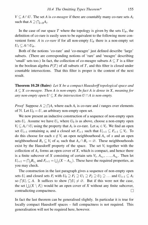
10.4 The Omitting Types Theorem* 155
V ⊆ A∩U . The set A is co-meagre if there are countably many co-rare sets Ai
such that A ⊇ ⋂∞i=0Ai.
In the case of our space T where the topology is given by the sets Uσ , thedefinition of co-rare is easily seen to be equivalent to the following more con-venient form: A is co-rare if for all non-empty Uσ there is a non-empty setUτ ⊆ A∩Uσ .
Both of the notions ‘co-rare’ and ‘co-meagre’ just defined describe ‘large’subsets. (There are corresponding notions of ‘rare’ and ‘meagre’ describing‘small’ sets too.) In fact, the collection of co-meagre subsets A ⊆ T is a filterin the boolean algebra P(T ) of all subsets of T , and this filter is closed undercountable intersections. That this filter is proper is the content of the nextresult.
Theorem 10.28 (Baire) Let X be a compact Hausdorff topological space andA ⊆ X co-meagre. Then A is non-empty. In fact A is dense in X, meaning forany non-empty open U ⊆ X the intersection U ∩A is non-empty.
Proof Suppose A ⊇ ⋂Ai where each Ai is co-rare and i ranges over elements
of N. Let U0 = U , an arbitrary non-empty open set.We now present an inductive construction of a sequence of non-empty open
sets Ui. Assume we have Ui, where U0 is as above, choose a non-empty openVi ⊆ Ai ∩Ui using the property that Ai is co-rare. Let ui ∈Vi. We find an openset Ui+1 containing ui and a closed set Fi+1 such that Ui+1 ⊆ Fi+1 ⊆ Vi. Todo this choose for each x �∈ Vi an open neighbourhood Ax of x and an openneighbourhood Bx ⊆ Vi of ui such that Ax ∩Bx = ∅. These neighbourhoodsexist by the Hausdorff property of the space. The set Vi together with thecollection of Ax forms an open cover of X , which is compact, and hence thereis a finite subcover of X consisting of certain sets Vi, Ax1 , . . . , Axk . Then letUi+1 =
⋂jBx j and Fi+1 =
⋃j(X −Ax j). These have the required properties, as
you may check.The construction in the last paragraph gives a sequence of non-empty open
sets Ui and closed sets Fi with U0 ⊇ F1 ⊇ U1 ⊇ F2 ⊇ U2 ⊇ . . . and Ui+1 ⊆ Ai
so⋂
Ui ⊆ A. It suffices to show⋂
Ui �= ∅. But if this were not the case,the set
⋃i(X \ Fi) would be an open cover of X without any finite subcover,
contradicting compactness.
In fact the last theorem can be generalised slightly. In particular it is true forlocally compact Hausdorff spaces – full compactness is not required. Thisgeneralisation will not be required here, however.

156 Completeness and compactness
The real power of Baire’s Theorem is that it shows that any countable inter-section of co-meagre sets is also co-meagre and hence non-empty. To see this,let Ai be co-meagre and Ai ⊇ ⋂
Ai j where each Ai j is co-rare. But N×N iscountable so there are in total a countable number of co-rare sets Ai j and hence⋂
iAi ⊇ ⋂i, jAi j which is non-empty by the Baire Theorem.
The next theorem connects these ideas with logic.
Theorem 10.29 The set of Σ+ ∈ Tmax with the Henkin property is a co-meagresubset of Tmax.
Proof Consider a formula φ(x) in a single free variable x. To ‘witness’ this xwith some c ∈ W we need to look at the Henkin sentence ∀x (¬φ(x)∨φ(c)).The set of Σ+ ∈ Tmax that makes this statement true is U∀x (¬φ(x)∨φ(c)). In fact,we do not mind which particular constant witnesses x in φ(x). The set ofΣ+ ∈ Tmax that witnesses x in φ(x) by some constant from W is the open setHφ(x) =
⋃c∈WU∀x (¬φ(x)∨φ(c)).
We stop a moment at this point to show that Hφ(x) is co-rare. Given a typicalnon-empty basic open set Uσ we need to consider Uσ ∩ Hφ(x). This set isopen; we need to show it is non-empty. Since Uσ is non-empty, Σ0 ∪ {σ}is consistent. But the sentence σ can only mention finitely many constantsc ∈ W . So some constant d ∈ W is not mentioned in σ , and so by the lemmaon Henkinisation (Lemma 10.4) σ ∧∀x(¬φ(x)∨φ(d)) is consistent. It followsby Zorn’s Lemma that this sentence is contained in some maximal Σ+ ∈ Tmax
and hence Σ+ ∈ Hφ(x) ∩Uσ , as required. Since this works for all Uσ , Hφ(x) isco-rare.
However, we are not interested in the set of Σ+ that witness φ(x) for a singleφ(x), but those that witness φ(x) for all φ(x). The set of these is
H =⋂
φ(x)Hφ(x)
which is a countable intersection of co-rare sets, hence co-meagre, since theset of all φ(x) is countable as LW is a countable language. This completes theproof
As mentioned, any countable intersection of co-meagre sets is co-meagre andhence non-empty. This suggests that we should find other co-meagre sets tointersect with the set of Σ+ having the Henkin property.
Definition 10.30 Let p be a set of L-formulas φ(x) in a single free variablex. Say that a set of LW -sentences Σ omits p if whenever c ∈ W is a constantsymbol then there is a formula φ(x) ∈ p such that ¬φ(c) ∈ Σ.

10.4 The Omitting Types Theorem* 157
We are going to find Σ ∈ Tmax with the Henkin property that omits one ormore sets p. However we will not be able to omit every set p. For example,when Σ0 is a theory of numbers and p is the set of all properties φ(x) true ofa prime x, then presumably p cannot be omitted as Σ0 already implies that theprime number x exists. More subtly, constructions using the Baire theorem areusually complex affairs with many parts happening ‘simultaneously’ and wemay not be able to omit p because some other part of the construction mayhave made some statement ∃x ψ(x) true and p is a set of properties true ofany x satisfying ψ(x). We define the class of p we can hope to omit in thefollowing definition.
Definition 10.31 Suppose p is a set of L-formulas φ(x) in a single free variablex, and Σ0 is a set of L-sentences. Say that p is isolated over Σ0 if there is someformula ψ(x) of L such that Σ0∪{∃x ψ(x)} ��⊥ and Σ0�∀x (ψ(x)→φ(x)) forall φ(x) ∈ p. Such a formula ψ(x) as here is said to be a support of p.
Lemma 10.32 Suppose p is a countable set of L-formulas with no supportover Σ0. Then the set of Σ+ ∈ Tmax which omits p is a co-meagre subset ofTmax.
Proof Start by looking at a single c ∈ W . We want this c to fail to satisfy allproperties in p. That is we want some ¬φ(c) to be true. That tells us to lookat the set
Sp, c =⋃
φ(x)∈pU¬φ(c).
The set of Σ+ in Sc are those that omit the set p at c. Let us show that Sc isco-rare. It is clearly open, so let σ be a sentence of LW and suppose Uσ isnon-empty. The sentence σ might involve c, so we write it as σ(c). Howeverthe sentence ∃x σ(x) is not a support of p, by our assumptions on p. So, asΣ0 ∪{∃x σ(x)} is consistent, by the definition of support there must be someφ(x) ∈ p such that Σ0 {∃x (σ(x)∧¬φ(x))} is consistent. But that means thatUσ(c)∧¬φ(c) = Uσ(c) ∩U¬φ(c) is non-empty, as required. The lemma now fol-lows as the set of Σ+ omitting p is
Sp =⋂
c∈WSp, c
which is a countable intersection of co-rare sets and hence is co-meagre.
Similar considerations apply to sets of first-order properties of a collection ofvariables.

158 Completeness and compactness
Definition 10.33 Suppose p is a set of L-formulas φ(x1, . . ., xk) in free vari-ables x1, . . ., xk, and Σ0 is a set of L-sentences. Then p is isolated over Σ0 ifthere is some formula ψ(x1, . . ., xk) of L such that Σ0 ∪{∃x ψ(x1, . . ., xk)} ��⊥and Σ0 �∀x (ψ(x1, . . ., xk)→φ(x1, . . ., xk)) for all φ(x1, . . ., xk) ∈ p. Such aformula ψ(x1, . . ., xk) is said to be a support of p. A set of LW -sentencesΣ omits p if whenever c1, . . ., ck ∈ W are constants from W then there isφ(x1, . . ., xk) ∈ p such that ¬φ(c1, . . ., ck) ∈ Σ.
Lemma 10.34 Suppose p is a countable set of L-formulas in free variablesx1, . . ., xk with no support over Σ0. Then the set of Σ+ ∈ Tmax which omits p isa co-meagre subset of Tmax.
Proof Identical to the previous proof, but using
Sp, c1, ..., ck =⋃
φ(x1, ..., xk)∈pU¬φ(c1, ..., ck)
and the fact that the set W k of k-tuples c1, . . ., ck of constants from W is alsocountable.
The reader can probably guess by now the terminology that is typically used insituations like this. A set p of formulas of the form φ(x1, . . ., xk) is often calleda ‘type’. (It represents a set of properties that may be held by some a1, . . ., ak ∈M, and hence represents a ‘kind’ or ‘type’ of k-tuple from M.) Also, a type isomitted by M if no tuple a1, . . ., ak ∈ M has the property represented by p.
If a type is not omitted in a structure M it is said to be realised in M. Ingeneral, omitting a type is the more difficult thing to do: realising a type simplyrequires the Compactness Theorem, as the next exercise shows.
Exercise 10.35 Let Σ0 be a consistent set of L-sentences, where L is a count-able first-order language, and for each n let p be a set of L-formulas of the formφ(x1, . . ., xkn) in free variables x1, . . ., xkn . Suppose that each pn is finitely sat-isfiable over Σ0, that is, for each finite q ⊆ pn there is Mq � Σ0 with somea1, . . ., akn ∈ Mq which satisfy every φ(x1, . . ., xkn) in q. Using the Compact-ness Theorem show that there is a single M � Σ0 in which none of the pn isomitted.
In contrast, the Omitting Types Theorem says that isolated types can beomitted. All that remains is to state this formally and put all the ingredientsabove together to give the proof.
Theorem 10.36 (Omitting Types) Let Σ0 be a consistent set of L-sentences,where L is a countable first-order language, and for each n ∈ N suppose that

10.4 The Omitting Types Theorem* 159
pn is a set of L-formulas φ(x1, . . ., xkn) in free variables x1, . . ., xkn and pn isisolated over Σ0. Then there is a countable L-structure M such that M �Σ0 andin which each pn is omitted.
Proof We will find a maximal Σ+ ∈ Tmax with the Henkin property. By Lemma10.26 this gives an LW -structure M � Σ+ in which every element is a constantfrom W . If in addition Σ+ omits each pn then each type pn is omitted by eachtuple of constants, and hence is omitted in M.
Thus we must find
Σ+ ∈ H ∩⋂
n∈NSpn
where H is the set of Σ+ with the Henkin property, in Theorem 10.29, and Spn
is the set of Σ+ that omits pn from Lemma 10.34. But this is a countable in-tersection of co-meagre sets, hence is non-empty by the Baire Theorem. Thussome Σ+ exists and we have proved the theorem.

11
Model theory
11.1 Countable models and beyond
Model theory is the study of arbitrary L-structures for first-order languages L.It is a sort of generalised algebraic theory of algebraic structures. We talk ofa structure M being a model of a set of L-sentences Σ when M � Σ, and thisgives the name to the theory. Actually, in practice, model theory tends to bemuch more about the structures themselves and the subsets and functions thatare definable in those structures by first-order formulas, and much less aboutfirst-order sentences, but the term ‘model theory’ seems to be fixed now. Thischapter attempts to give a flavour of model theory and presents some of thefirst theorems. It also contains a considerable amount of preliminary materialon countable sets and cardinalities that we have somehow managed to put offuntil now.
Model theory starts off with the Compactness Theorem for first-order logic,which is phrased entirely in terms of the notion of semantics, �, but was provedin the last chapter by an excursion into the realm of formal proofs. The keyresult guaranteeing the existence of models of a set of sentences Σ is the Com-pleteness Theorem for first-order logic which provides us with a model M of Σ,under the assumption that Σ � �⊥. We will start by looking at the CompletenessTheorem in a little more detail to see what extra it can say for us.
The construction of the model M that the proof of the Completeness Theo-rem gives us is rather mysterious, as it relies on Zorn’s Lemma to do the workof finding the maximal set extending Σ, and aside from choosing the sentencesin Σ in the first place, we have little input. It is natural to ask a little more aboutthis structure M we end up with.
As it happens, we cannot really say very much more about it: most questionsabout M that can be settled at all are answered by looking at the initial data Σ.In other words, almost all we know about M is the Σ that we started with.
160
11.1 Countable models and beyond 161
If you need a particular M with special properties it is usually necessary tostart with a different Σ (possibly in a different language) or, for more advancedwork, apply more sophisticated variations of the Henkin construction givenabove such as the Omitting Types Theorem of Section 10.4. One of the fewexceptions to this rule is the ‘size’ or cardinality of M. This is what we shallstart our study of model theory with here.
We shall start with the countable case, and then explain how similar resultsapply in other infinite cases. As the discussion of uncountable structures in-evitably involves some set theoretic background, the key technical results willbe stated here but proved in an optional section, later on in this chapter.
The idea of a countable set was introduced earlier, in Definition 2.13. Ourdefinition said that a set X is countable if it is empty or if there is a surjectionfrom N to X . There is an alternative that is also convenient at times, indicatedin the following proposition.
Proposition 11.1 A set X is countable if and only if there is an injectionf : X →N.
Proof Suppose X is countable. Then if X is empty, by convention the emptyfunction f from X to N is a perfectly good injection. (We do not have tospecify any values f (x) because there are none.) Otherwise, suppose g: N→Xis a surjection. Then we can define f : X →N by letting f (x) be the least n ∈ N
such that g(n) = x. This is well defined as g is onto X , and is clearly aninjection as no two distinct x, y ∈ X can receive the same n since this wouldmean x = g(n) = y.
Conversely, if f : X →N is an injection, then if X is empty it is countable, sosuppose not. Choose x0 ∈ X and let g(n) = x0 if n �∈ im( f ) and let g(n) be theunique x ∈ X such that g(x) = n otherwise. It is easy to check that this definesa surjection g: N→X .
We are mainly interested in infinite countable sets, also called countably infi-nite sets. The canonical example of such a set is the set N of natural numbers.However, many other such sets are countable, and there are some surpriseshere too. We start with some reasonably pleasant consequences of our notionof ‘countable’.
Proposition 11.2 Let A be a countable set and f : A→B a bijection. Then B iscountable.
Proof If A is empty, then B must be too, for otherwise f cannot be surjective.

162 Model theory
And if g: N→A is a surjection then the composition of g and f is a surjectionN→B.
Proposition 11.3 Any subset of a countable set is countable.
Proof If A is countable and f : A→N is an injection, then for each B ⊆ A therestriction of f to B is also an injection B→N.
Proposition 11.4 If A is a countable set and ∼ is an equivalence relation onA then the set A/∼ of equivalence classes of A is countable.
Proof Suppose f : N→A is a surjection and define g: A→A/∼ by g(a) = a/∼,the equivalence class of a. Then the composition of f and g is a surjectionN→A/∼.
Proposition 11.5 If A and B are countably infinite sets then there is a bijectionf : A→B.
Proof We suppose A is countably infinite and show that there is a bijectiong: N→A. The result will follow from a similar fact about B and by composingbijections.
So suppose h: A→N is an injection. Then im(h) cannot be empty nor have alargest element n, for if it did, A would have at most n+1 elements and wouldbe finite. Thus im(h) contains arbitrarily large natural numbers and there is afunction k: N→N such that k(0) is the first element of im(h), k(1) is the secondelement of im(h), . . ., and k(n) is the n+1st element of im(h). (This functionk is defined inductively by k(0) is the least element of im(h) and k(n + 1) isthe least element of im(h)∩{m ∈ N : m > k(n)}.) Then the function g: N→Adefined by g(n) = h−1(h(n)) is a bijection.
The surprise comes next.
Proposition 11.6 If A, B are countable sets then their union A∪B and carte-sian product A×B are both countable.
Proof Suppose f : A→N and g: B→N are injections.We can define an injection h: A ∪ B →N by h(x) = 2 f (x), if x ∈ A, and
h(x) = 2g(x)+ 1, if x �∈ A. It is easy to check this is also an injection, henceA∪B is countable.
For the cartesian product, note that the function p: N×N→N given by

11.1 Countable models and beyond 163
�x
�
y
0 1 2 3 4 · · ·
0 0 � 1�
��
3�
��
6�
��
10�
��1 2������
4�
��
7�
��
11�
��2 5
��
��
���
8�
��
12�
��3 9
�
13���
4 . . .
...
Figure 11.1 A pairing function for the natural numbers.
p(x, y) = (x + y)(x + y + 1)/2 + y is in fact a bijection pairing up two naturalnumbers as a single number. This is because (x + y)(x + y + 1)/2 gives thenumber of points (r, s) ∈ N×N for which r + s < x + y and thus the pairsmapping to values between k(k + 1)/2 and (k + 1)(k + 2)/2− 1 are the pairs(x, y)∈N×N with x+y = k (see Figure 11.1). Thus we can define an injectionk: A×B→N by k(a, b) = p( f (a), g(b)), showing A×B is countable.
The first time you see this, it is quite startling news. For example, this propo-sition implies that Z and Q are countable. Z is countable because it is thedisjoint union of two copies of N (namely the non-negative and the nega-tive integers) and Q is countable since it can be constructed as a quotient ofthe set Z× (Z \ {0}). The countability of the set of Z and Q seems to becounter-intuitive as Q contains so many more elements than N, but as we cannow see Q and N turn out to be exactly the same size.
These simple propositions on countability are enough to sharpen the Com-pleteness Theorem quite considerably.
Definition 11.7 A countable first-order language is a first-order language L inwhich the set of variables, the set of constants, the set of relation symbols, andthe set of function symbols, are all countable.

164 Model theory
Proposition 11.8 Let L be a countable first-order language. Then there arecountably many finite strings of symbols from L.
Proof We use the bijection p: N×N→N of Proposition 11.6, and extend it tobijections pk: Nk →N by defining p1(n) = n and
pk+1(n1, n2, . . ., nk, nk+1) = p(pk(n1, n2, . . ., nk), nk+1).
Now given an injection f : L→N from the set of symbols of L to N, we defineg from strings σ1σ2. . .σk of L-symbols σ1, σ2, . . ., σk to natural numbers by
g(σ1σ2. . .σk) = p(k, pk( f (σ1), f (σ2), . . ., f (σk)))
and it is easy to check this is an injection.
Proposition 11.9 Let L be a countable first-order language. Then the com-plete Henkinisation LH is countable, and the set of closed terms of LH is alsocountable.
Proof It suffices, by the previous proposition, to show that there are countablymany symbols in LH , for the set of closed terms in this language is a set ofstrings from these symbols.
Now there are countably many strings of the form φ(x) from L, and so thefirst Henkinisation H(L) consists of a union of a countable set of symbols Land an additional countable set
{εφ(x) : φ(x) from L
}. So H(L) is countable
by Proposition 11.6, and what is more this process gives a completely definitemethod for obtaining an injection H( f ): H(L)→N from an injection f : L→N.
To define an injection LH →N, take a symbol s of LH and let n ∈ N be leastsuch that s is in the nth Henkinisation Hn(L) of L. Then we define g(s) =p(n, Hn(s)), the number for the pair consisting of n and the number for thesymbol s in Hn(s).
Definition 11.10 An L-structure M is said to be countable if its domain orunderlying set is countable.
Theorem 11.11 (Completeness Theorem, countable version) Let Σ be a setof sentences in a countable first-order language L, and suppose that Σ � � ⊥.Then there is a countable model of Σ.
Proof Just repeat the previous proof of the Completeness Theorem, notingthat the structure obtained has domain which is a quotient of the set of closed

11.1 Countable models and beyond 165
terms of the Henkinised language, so is countable by Proposition 11.9 andProposition 11.4.
This new version of the Completeness Theorem is quite striking too. For ex-ample, consider the structure R consisting of the real numbers together withthe constants 0, 1, the functions +, ×, −, and the relation <. The correspond-ing first-order language L is countable. Now let Σ be the set of all L-sentencestrue in R. By the Soundness Theorem Σ � �⊥, so by the countable form of theCompleteness Theorem Σ has a countable model. This cannot be R itself, as R
is uncountable.Even more disconcertingly, it is possible to express all our axioms of set the-
ory, the Zermelo–Frankel theory of sets, in a countable first-order language. InZermelo–Frankel set theory it is possible to discuss and prove all of our re-sults on countability and uncountability – including the uncountability of R.It follows that there is a countable model M of set theory, with its own count-able version of R, that makes the statement ‘R is uncountable’ true. Thisparadox is known as ‘Skolem’s paradox’. It is resolved by observing that thenotions of ‘countable’ in our M and in the real world are actually rather dif-ferent. Rather than concluding that we cannot in fact talk about countable anduncountable sets in any coherent way, it is perhaps better to conclude that acountable first-order language is not actually expressive enough to capture ournotion of countability in the real world correctly.
We now turn to other infinite sets, such as the set of real numbers, whichwas shown to be uncountable by Cantor (see Exercise 2.28). We will needsome results on the sizes of these sets analogous to our results on countablesets, and as these results are really ‘set theory’ rather than ‘logic’ we shall notprove them here. They can all be proved from Zorn’s Lemma, and proofs aregiven in an optional section in this chapter. The size of a set will be calledits cardinality, and we will need to compare cardinalities, saying when twocardinalities are equal, or when one is larger than the other. The next twodefinitions explain this.
Definition 11.12 Two sets A and B have the same cardinality if there is abijection f : A→B.
Definition 11.13 Let A and B be sets. We write cardA � cardB to mean thereis an injection f : A→B. We write cardA < cardB to mean there is an injectionf : A→B but no bijection g: A→B.
A very special case of this is that of 0, the cardinality of the empty set: this

166 Model theory
is less than or equal to all other cardinalities, since there is always an injectionfrom ∅ to any other set, the empty function, as discussed earlier.
Remark 11.14 Definitions 11.12 and 11.13 beg a difficult question: whatmathematical object is the cardinality of a set? In fact nothing later on willrequire a specific answer to this question, so unless you are curious, this re-mark can be safely skipped. But there are perfectly reasonable definitions of‘cardinal’. One attempt goes as follows. As the relation of ‘having the samecardinality’ is an equivalence relation on the class of all sets, the cardinalitycardA of a set A should be the equivalence class of A under this relation. Thatwill be good enough for us here, but it is not quite right since – as it happens –this equivalence class is not a set in the official sense of Zermelo–Frankel settheory. A technical variation of this definition (known as Scott’s trick) doessucceed in defining a set cardA representing the cardinality of A as the equiva-lence class of all sets in a specially chosen sub-universe of sets containing setsof the same cardinality as A. With the Axiom of Choice there are several moreattractive alternative definitions of cardA, including defining it to be the leastordinal in one-to-one correspondence with A, so the problem can be resolved,though not without going somewhat beyond the scope of this book.
Definition 11.15 For a finite set A with n elements we let cardA = n and,following the notation first given by Cantor, if A is a countably infinite set wewrite ℵ0 for the cardinality cardA, where ℵ is the first Hebrew letter ‘aleph’.
The next three propositions explore the � relation further; they do not seemvery surprising, but should not be belittled. None of these propositions is ob-vious or straightforward to prove. Proofs appear later in the optional section.
Proposition 11.16 Suppose there is a surjection f : A→ B. Then cardB �cardA, i.e. there is an injection g: B→A.
Proposition 11.17 (Schroder–Bernstein Theorem) Let A and B be sets andsuppose that cardA � cardB and cardB � cardA; then cardA = cardB. Inother words if there are injections A→B and B→A then there is a bijectionA→B.
Proposition 11.18 (Trichotomy Theorem) Let A and B be sets. Then exactlyone of the following is true: cardA < cardB; cardA = cardB; or cardB <
cardA.
There are results analogous to earlier propositions on countable sets for ar-
11.1 Countable models and beyond 167
bitrary cardinalities. For example, if A ⊆ B then cardA � cardB since themap a �→ a is an injection A→B. If ∼ is an equivalence relation on A thencard(A/∼) � cardA as the map a �→ a/∼ is a surjection A→A/∼ and wemay apply Proposition 11.16 to obtain an injection A/∼→A. Here is anotherapplication of the above results.
Proposition 11.19 Let A be infinite. Then ℵ0 � cardA, i.e. there is an injectionN→A.
Proof By trichotomy, if the conclusion is false then cardN > cardA. Thiswould mean that there is an injection f : A→N but no bijection between Aand N. This is impossible since A is infinite, so the image im f ⊆ N is alsoinfinite and any infinite subset of N is in one-to-one correspondence with thewhole of N, by Proposition 11.5, which would mean A is also in one-to-onecorrespondence with N.
We are interested in uncountable versions of the Completeness Theorem. Forthat we need to compute the number of symbols in the complete HenkinisationLH of an uncountable language L. To do this we will need to add and multiplyinfinite cardinalities.
Definition 11.20 Let A, B be sets, and κ = cardA, λ = cardB. Then
(i) κ +λ is the cardinality of the set (A×{0})∪ (B×{1}),(ii) κλ is the cardinality of the set A×B.
Proposition 11.21 The cardinal arithmetic operations of addition and multi-plication are well defined. That is, they do not depend on the choice of setsA, B.
Proof Suppose cardA = cardA′ and cardB = cardB′, so there are bijectionsf : A→A′ and g: B→B′. Then
h: (A×{0})∪ (B×{1})→ (A′ ×{0})∪ (B′ ×{1})defined by
h(a, 0) = ( f (a), 0) ∈ A′ ×{0} and h(b, 1) = (g(b), 1) ∈ B′ ×{1}for a ∈ A and b ∈ B, is a bijection, since f , g are. (Exercise: verify this.) Also,
k: A×B→A′ ×B′

168 Model theory
defined by
k(a, b) = ( f (a), g(b)) ∈ A′ ×B′
is also a bijection. Thus card(A×{0}∪B×{1}) = card(A′ ×{0}∪B′ ×{1})and card(A×B) = card(A′ ×B′).
Other natural properties of cardinal arithmetic such as associativity, commuta-tivity and distributivity also work as you might expect. For infinite cardinali-ties, these operations are quite straightforward, and the next proposition is ourkey result for calculating the cardinality of LH . Again, it is not at all easy, anda proof from Zorn’s Lemma will be found in an optional section later on.
Theorem 11.22 (Cardinal Arithmetic) Let A, B be infinite sets, and κ =cardA, λ = cardB. Then κ +λ = κλ = max{κ, λ}.
With all these preliminaries out of the way, we can get back to logic. Sinceproofs are finite objects, there is never any need for more than countably manyvariable symbols in a first-order language, so from now on we shall assume allof our first-order languages have countably many variables.
Definition 11.23 Let L be a first-order language. Then the cardinality cardLof L is the cardinality of the set of symbols in L. In other words, using Theo-rem 11.22, cardL is the maximum of: (a) ℵ0; (b) the cardinality of the set ofconstant symbols of L; (c) the cardinality of the set of relation symbols of L;(d) the cardinality of the set of function symbols of L.
Proposition 11.24 Let L be a first-order language. Then the cardinality of theset of strings of symbols from L equals cardL
Proof This is similar to the countable case, but using the proposition on cardi-nal arithmetic instead of a directly constructed pairing function.
Let S be the set of symbols from L, so cardS = κ is infinite. By cardinalarithmetic (Theorem 11.22) there is a bijection p: S×S→S. We extend this topk: Sk →S by p1(s) = s and
pk+1(n1, n2, . . ., nk, nk+1) = p(pk(n1, n2, . . ., nk), nk+1).
Also, as S is infinite, there is an injection q: N→ S, by Proposition 11.19. Sowe may define g from strings of symbols of L to S by
g(σ1σ2. . .σk) = p(q(k), pk(σ1, σ2, . . ., σk))
and this is readily seen to be an injection.

11.1 Countable models and beyond 169
Proposition 11.25 Let L be a first-order language. Then the cardinality of thecomplete Henkinisation LH of L is the same as that of L; the cardinality of theset of closed terms of LH is also equal to cardL.
Proof This proof is almost identical to the countable case, Proposition 11.9.Let κ = cardL. It suffices to show that there are κ many symbols in LH .
Now there are κ many strings of the form φ(x) from L, and so the firstHenkinisation H(L) consists of a disjoint union of L with a set of constantsymbols
{εφ(x) : φ(x) from L
}of cardinality κ . So cardH(L) = κ +κ = κ by
cardinal arithmetic, and this gives a bijection h1: H(L)→L from the symbolsof H(L) to the symbols of L. Similarly we can choose for each k ∈N a bijectionhk: Hk(L)→L from the symbols of the kth Henkinisation of L to the symbolsof L. We also have, by Proposition 11.19 and cardinal arithmetic, an injectionp: N×L→L.
Now, to define an injection LH → L, take a symbol s of LH and let k ∈ N
be least such that s is in the kth Henkinisation Hk(L) of L. Then define a mapg(s) = p(k, hk(s)) taking the symbol s to a symbol in L ‘encoding’ the pairconsisting of k and the symbol s. This is readily seen to be an injection.
Definition 11.26 The cardinality of an L-structure is the cardinality of itsunderlying set, i.e. the cardinality of the non-empty domain of elements of thestructure.
Theorem 11.27 (Completeness Theorem, arbitrary cardinalities) Let Σ bea set of sentences in a first-order language L, and suppose that Σ � �⊥. Thenthere is a model of Σ of cardinality at most cardL.
Proof Just repeat the previous roof, noting that the domain of the structure itgives is a quotient of the set of closed terms of the Henkinised language, andtherefore has cardinality at most this.
It does not take very much work to modify this result to obtain models of allpossible infinite cardinalities. All we need is an additional assumption thatour set Σ has some infinite model. More specifically, we use the followingtheorem.
Theorem 11.28 Let Σ be a consistent set of sentences in a first-order languageL, let κ � cardL, and suppose that Σ has at least one infinite model. Then Σhas an infinite model of cardinality κ .

170 Model theory
Proof Let Cκ be a set of constants of cardinality κ and let L+ be the languageL with these constant symbols added. Then cardL+ is exactly κ , by cardinalarithmetic. Also, let Tκ be the set of all statements ¬c = d for c �= d ∈ Cκ .Observe that Tκ ∪Σ is consistent. This is because in any infinite model M of Σ,any finite subset of constants from Cκ can be interpreted in M in a way makingthem all different.
It follows by the Completeness Theorem that there is a model Mκ � Tκ ∪Σof cardinality at most κ . That is, there is an injection M →C, where C is ourset of new constants which has cardinality κ . But by the statements Tκ , themap c �→ [c] taking the constant symbol c ∈ C to the element of M realisingit, i.e. to the equivalence class of c, is also an injection C→M. It follows bythe Schroder–Bernstein Theorem that there is a bijection C →M and hencecardM = cardC. By discarding the additional constants in Cκ we obtain anL-structure of cardinality κ making Σ true.
At last, we can do some model theory and give an application of these ideasto mathematical theories formalised in first-order languages. First, we need adefinition.
Definition 11.29 Let L be a first-order language and Σ be a set of L-sentences.We say that Σ is complete (for L) if whenever σ is an L-sentence we have eitherΣ�σ or Σ�¬σ .
This should not be confused with the Completeness Theorem. The Com-pleteness Theorem says that our logic is complete, i.e. can prove all valid as-sertions. Think of Σ as a mathematical theory, such as a theory of groups,formalised in a first-order language L using first-order logic. Then Σ is com-plete if it can decide all mathematical statements that can be expressed in L, forexample our theory of groups is complete if it decides all first-order statementsabout groups.
Example 11.30 Let L be the first-order language with the usual logical sym-bols, including =, but with no additional logical symbols. Let σn be an L-sentence expressing the fact that there are at least n elements (see Exercise10.7). Let Σ = {σn : n ∈ N}. Then it turns out that Σ is complete, i.e. for everyσ in L either Σ�σ or Σ�¬σ . (We will prove this in a moment.) On the otherhand, no finite subset Σ0 of Σ is complete since, given Σ0 there is always somen ∈ N such that Σ0 � �σn and Σ0 � �¬σn as we may take models of any particularfinite cardinality above some minimum cardinality determined by Σ0.
Complete sets Σ are of interest for many reasons, not least in the study of the

11.1 Countable models and beyond 171
foundations of mathematics, where complete sets provide examples of math-ematical theories where all mathematical statements (in the appropriate lan-guage) can be determined true or false by a formal proof. It was a sort ofHoly Grail of logic in the early twentieth century to find a proof system forthe whole of mathematics, or a large part of it such as number theory or settheory, that was complete for its language. Such a system would, in principle,put mathematicians out of work, to be replaced by a computer churning outtheorems in the system. That this Grail is in fact unattainable was eventuallyproved by Godel in 1931. However, in looking for such theories a number ofpeople, such as Tarski and Hilbert, found interesting first-order systems thatwere complete for their (limited) languages.
In a way exactly analogous to isomorphisms in traditional algebraic con-texts, we say that two models M, N for the same language L are isomorphic ifthere is a bijection from M to N that preserves the L-structure on M, N. Suchisomorphisms necessarily preserve the truth of L-sentences. (A formal proofof this fact is an induction on the number of symbols in a formula, and is leftas an exercise for the pedantic reader.) We now use this idea to give anotherimportant model theoretic notion.
Definition 11.31 Let L be a first-order language, Σ be a set of L-sentences,and κ an infinite cardinal. We say Σ is κ-categorical if all models of Σ ofcardinality κ are isomorphic to each other.
Theorem 11.32 Let L be a first-order language, and Σ be a set of L-sentences.Suppose Σ is κ-categorical for some infinite cardinal κ � cardL and Σ has nofinite models. Then Σ is complete.
Proof If Σ is not complete there is an L-sentence such that both Σ1 = Σ∪{σ}and Σ2 = Σ∪{¬σ} are consistent. Since Σ has no finite models, by Theorem11.28 there are models M1 �Σ1 and M2 �Σ2 of cardinality κ . But these modelscannot be isomorphic since they do not agree about the truth of the sentenceσ , so Σ is not κ-categorical.
Example 11.33 The set Σ of Example 11.30 is complete, as any two countablyinfinite models for the language with no non-logical symbols are necessarilyisomorphic, and Σ has no finite models.
Theorem 11.32 gives interesting information in the following example.
Example 11.34 Let F be a field, such as R, and consider infinite vector spaces

172 Model theory
over F . We will present a first-order language LF for such vector spaces. LF
has binary function + for addition of vectors, unary function − for additiveinverses, and a constant symbol 0 for the zero vector. It also has, for eachλ ∈ F , a unary function sλ for scalar multiplication by λ . It is possible towrite down a set ΣF of first-order axioms for F-vector spaces in this language(Exercise 11.37). Note that our language works for a fixed F only, and thereare no symbols for addition or multiplication in F .
Then ΣF is complete, since there are models of ΣF of every infinite cardinal-ity κ � cardF , and any two vector spaces of cardinality κ > cardF have basesof cardinality κ and hence are isomorphic. See also Exercises 2.32, 2.33, and11.38.
This example is rather good in that it gives the flavour of the subject fromthis point. There is a huge amount of extra information to be gleaned from thealgebraic arguments on vector spaces and the logical information on the theoryof F-vector spaces. It is possible to classify, for example, all the possibleformulas in our language of F-vector spaces, what they say and what they candefine.
The example of F-vector spaces is typical in one other important regard, inthat it is categorical for all cardinalities greater than the cardinality of the lan-guage. A remarkable theorem due to Morley shows that this is generally truefor theories categorical in some cardinality greater than that of their language.
Theorem 11.35 (Morley) Let T be a set of sentences in a language L andsuppose that T has no finite models. Suppose further that T is κ-categoricalfor some cardinality κ > cardL. Then T is κ-categorical for all cardinalitiesκ > cardL.
A proof of Morley’s Theorem is well beyond the scope of this book. Oneproof goes by trying to associate a notion of dimension to a model of T . Thenby some subtle generalisation of the argument for vector spaces a model of Tis determined exactly by its dimension, which for cardinalities greater than thatof the language can only be the same as the cardinality of the whole model.
Model theory says a lot about theories of dimension for rather general L-structures. In particular, a set of sentences Σ in a countable language which isκ-categorical for all uncountable κ will have the property of being ω-stable,and ω-stable structures have an elegant independence and dimension theorythat generalise the idea of independence in a vector space. More generally,there is a slightly weaker notion of a stable structure which includes ω-stablestructures as a special case, and stable structures also have an elegant (but notin general quite so well behaved) notion of independence. For example, the

11.2 Examples and exercises 173
first-order theory of modules over a ring R is a stable theory with a nice notionof independence, that generalises and includes the idea of independence in avector space over a field as a special case. Stability theory is a large branch ofmodel theory that tries to analyse and classify algebraic theories of groups,rings, fields, modules, according to their properties concerning the model-theoretic notion of stability and these corresponding independence properties,and say something useful about these theories, such as what sets are definableby first-order formulas in the language.
For further information on model theory the reader should consult a moreadvanced text, such as the one by Marker [9].
11.2 Examples and exercises
Exercise 11.36 (a) Let A be a set of circular discs in the plane, no two of whichintersect. Show that A is countable.
(b) Let B be a set of circles in the plane, no two of which intersect. Showthat B may be uncountable.
(c) Let C be a set of figures-of-eight in the plane, no two of which intersect.Can C be uncountable?
Exercise 11.37 Write down the axioms for infinite F-vector spaces in thelanguage LF of Example 11.34. (Note that, to ensure the models of this theoryare all infinite, it may be necessary to add the statements σn of Example 11.30.)
Exercise 11.38 Suppose V is an F-vector space of cardinality κ > cardF . LetB be a basis of V . Show that cardB = κ . What can happen when κ = cardF?
Definition 11.39 The theory DLO (for Dense Linear Orders) has single binaryrelation < and axioms
• ∀x∀y∀z (x < y∧ y < z→ x < z)• ∀x¬(x < x)• ∀x∀y (x < y∨ x = y∨ y < x)• ∀x∃y∃z (x < y∧ z < x)• ∀x∀y (x < y→∃z (x < z∧ z < y))
For example, the structures (Q, <) and (R, <) both satisfy DLO.
Exercise 11.40 Prove that DLO is ℵ0-categorical.(Hint: prove that a countable model (A, <)�DLO is isomorphic to (Q, <)
174 Model theory
by building an isomorphism A→Q inductively. At any stage in the construc-tion we have n distinct elements a1, a2, . . ., an of A and n distinct elementsq1, q2, . . ., qn of Q. Inductively assume ai < a j if and only if qi < q j for alli, j, i.e. the ai can be ordered as ai1 < ai2 < .. . < ain with the qi ordered by thesame indices, qi1 < qi2 < .. . < qin . Show how the DLO axioms allow, givensome new an+1 from A, a new element qn+1 to be added to the qi list with theinduction hypothesis preserved, and that, given some new qn+2 from Q, a newelement an+2 to be added to the ai list with the induction hypothesis preserved.(These two steps are traditionally called ‘back-and-forth’.) Explain also howthe countability of A and Q, and hence enumerations of each, allow this induc-tive back-and-forth construction to build an isomorphism between (A, <) and(Q, <).)
Exercise 11.41 Explain why the previous exercise shows that DLO is completefor its language.
Exercise 11.42 Find sets of sentences Ta, Tb, Tc, Td in countable languagesLa, Lb, Lc, Ld such that none of Ta, Tb, Tc, Td has any finite models, and
• Ta is κ-categorical for all infinite κ ,• Tb is κ-categorical for all infinite κ > ℵ0 but is not ℵ0-categorical,• Tc is ℵ0-categorical but is not κ-categorical for any κ > ℵ0,• Td is not κ-categorical for any infinite κ .
(Hint: for Tc consider the theory DLO. Why is it not κ-categorical for κ > ℵ0?)
A formula of the language of DLO can always be rewritten without the ¬sign. For example, ¬x = y is equivalent in DLO to x < y∨ y < x and ¬(x < y)is equivalent in DLO to x = y∨ y < x. We shall see soon that the quantifiers ∀and ∃ can also be eliminated.
Definition 11.43 A formula is said to be quantifier free if it contains neither ∀nor ∃.
Exercise 11.44 Using induction on the number of connectives of θ , prove thatany quantifier free formula θ which only uses connectives ∨ and ∧ is logicallyequivalent to a formula of the form
∨k
r=1
∧lrs=1
φr, s
where each φr, s is atomic, i.e. is an equation t1 = t2 or is R(t1, t2, . . ., tn) forsome relation symbol R.
11.2 Examples and exercises 175
A number of theories have the property that all formulas are equivalent inthem to a quantifier free formula. The process showing this is called elimi-nation of quantifiers. When a theory has elimination of quantifiers we usuallyhave a nice description of sets that are definable in models of the theory. Quan-tifiers are not eliminated from the discussion completely: they are still neededin the axioms of the theory, for example. Also, from the point of view of de-scribing the set defined by a formula, adding an existential quantifier ∃xn . . .
to a formula φ(x1, . . ., xn−1, xn) corresponds to a projection of the set onto thefirst n − 1 coordinates. Elimination of quantifiers shows that the quantifierfree definable sets are closed under projection functions, and this is often verypowerful.
We will illustrate this with the theory DLO. The following lemma containsthe main step in the elimination of quantifiers for DLO.
Proposition 11.45 Suppose a formula θ(x1, . . ., xk) of the language of DLO isof the form
∃y∧k
n=1φn(y, x1, . . ., xk)
where each φn is either ‘xi < y’, ‘y < xi’, ‘y = xi’, ‘xi = x j’, or ‘xi < x j’, forsome i, j. Then θ is equivalent (in the theory DLO) to a formula which isquantifier free.
Proof If some φn is ‘y = xi’ then we may replace y throughout with xi andremove the quantifier. So assume that the φn involving y are all of the form‘xi < y’, or ‘y < xi’, and let L be the set of indices of lower bounds,
L = {i : some φn is xi < y} ,
and U be the set of indices of upper bounds,
U = {i : some φn is y < xi} .
Also, let A = {n : φn does not involve y}. The more interesting case is when Land U are both non-empty, and in this case we try to rewrite θ as∧
n∈Aφn ∧
∧i∈L
∧j∈U
xi < x j.
I have to explain why this statement is equivalent to θ .The easiest way to do this is to think about a specific model of DLO with
specific elements x1, . . ., xk in our model and argue that for these the equiva-lence of θ and the statement above holds. Then by the Completeness Theo-rem and by the fact our model and elements x1, . . ., xk were arbitrary we havethat the equivalence is provable in DLO. But there are finitely many elements

176 Model theory
x1, . . ., xk in our list, so from {xi : i ∈ L} there is a maximum element (as theorder is linear), and from {xi : i ∈U} there is a minimum element. The state-ment
∧i∈L
∧j∈U xi < x j says that max{xi : i ∈ L} is less than min{xi : i ∈U}.
So by an axiom of DLO there is some y between these. Therefore, if all theφn not involving y are also true, we deduce that θ(x1, . . ., xn) is true, and thisshows one direction of the equivalence of the formula above with θ . The otherdirection is easier since if there is y such that xi < y for all i ∈ L and y < x j forall i ∈U then xi < x j for all i ∈ L, j ∈U by transitivity.
In the cases when U or L is empty, we claim that θ is equivalent in DLO to∧n∈Aφn, and use another axiom of DLO (the one that states there is no least or
greatest element) to find a y such that y is greater than all xi for i ∈ L (in thecase when U = ∅) or to find a y such that y is less than all x j for j ∈U (in thecase when L = ∅).
Exercise 11.46 Using induction on the number of quantifiers in a statement θ ,and also Exercise 11.44 and Proposition 11.45, show that every formula θ inthe language of DLO is equivalent in DLO to a quantifier free formula in thesame language with the same free variables.
(Hint: treat the universal quantifier ∀y . . . by converting it to an existentialone ¬∃y¬ . . ..)
Definition 11.47 A subset A of a model M is definable if there is a formulaθ(x, y1, . . ., yk) of the language of M and parameters a1, . . ., ak ∈ M such that
A = {b ∈ M : M �θ(b, a1, . . ., ak)} .
Exercise 11.48 Show that every definable set in a model of DLO can bedescribed as a disjoint union of singleton sets {a} and intervals of the form(a, b) = {x : a < x∧ x < b} or (a, ∞) = {x : a < x} or (−∞, b) = {x : x < b}.
11.3 Cardinal arithmetic*
The object of this section is to provide the proofs of the various results on car-dinal arithmetic that were needed above. With the exception of the Schroder–Bernstein Theorem, they all require Zorn’s Lemma in some form or other. Allof the results here are ‘set theory’ rather than logic and although the results areimportant for more advanced model theory they may be taken on trust.
We will start by giving Tarski’s proof of the Schroder–Bernstein Theorem.The idea is that, given sets A and B and injections f : A→B and g: B→A wewould like to partition A = A0 ∪A1 and B = B0 ∪B1 so that f : A0 →B0 and

11.3 Cardinal arithmetic* 177
g: B1→A1 are onto, for then we could define h: A→B as h(a) = f (a) if a ∈ A0
and h(a) = g−1(a) if a ∈ A1. To get this to work we need to find A0, andyou should note that A0 would have to satisfy A0 = A \ g(B \ f (A0)). Thefollowing lemma is designed to provide us with such a set A0.
Lemma 11.49 (Tarski’s Fixed Point Lemma) Let A be any set and let k bean order preserving map k: P(K)→P(K) defined on the power set P(K) ={U :U ⊆ K} of U, where ‘order preserving’ means that if X ⊆ Y ⊆ A thenk(X) ⊆ k(Y ). Then there is some A0 ⊆ A such that k(A0) = A0.
Proof The idea is to define A0 to be the ‘limit’ (or more precisely, the union) ofall sets X ⊆ A which are too small in the sense that X ⊆ k(X). More precisely,let A0 =
⋃T where T = {X ⊆ A : X ⊆ k(X)}.
Then if X ∈ T then X ⊆A0 so X ⊆ k(X)⊆ k(A0). This shows that A0 ⊆ k(A0)since each x ∈ A0 is in some X ∈ T . Also, as k is order preserving and A0 ⊆k(A0) we have k(A0) ⊆ k(k(A0)) so k(A0) ∈ T , showing that k(A0) ⊆ A0.
Proof of the Schroder–Bernstein Theorem Given sets A and B and injectionsf : A→B and g: B→A, define a map from k: P(A)→P(A) by
k(X) = A \ g(B \ f (X)),
and verify that it is order preserving. By Tarski’s Lemma there is a fixed pointA0 ⊆ A. Given this we may define A1 = A \ A0 and h: A→B as h(a) = f (a) ifa ∈ A0 and h(a) = g−1(a) if a ∈ A1. It is straightforward now to check that his a bijection from A to B.
The next result shows that in almost all cases we could have defined the ‘lessthan’ operation on cardinals in terms of surjections rather than injections. (Thecase that would not work is that of the empty set.) Despite its apparent sim-plicity the Axiom of Choice or Zorn’s Lemma is necessary here.
Proposition 11.50 Suppose f : A→B is a surjection. Then cardB � cardA,i.e. there is an injection g: B→A.
Proof Let S be the set of all injections g: U →A such that U ⊆ B and f (g(b)) =b for all b ∈U . Order S by the idea of extending functions, i.e. say that g � hif and only if domg ⊆ domh and g(x) = h(x) for all x ∈ domg. Then theempty function is in S and S has the Zorn property as all functions in a chainof elements of S are ‘compatible’ so the union of this chain is also an injectionfrom some subset of B to A satisfying the required condition.

178 Model theory
By Zorn’s Lemma there is a maximal injection g: U →A such that f (g(b)) =b and we may check that U = B. For if not then there is b ∈ B \U and b = f (a)for some a ∈ A as f is surjective. Then we may define h(x) = x if x ∈ U andh(b) = a. This would be an extension of g in S, but g is maximal so there canbe no such extension. Therefore U = B as required.
If X is a non-empty set and ∼ an equivalence relation on X then there is alwaysa surjection X→X/∼ given by x �→ [x], so a quotient by an equivalence relationalways has the same or smaller cardinality than the original set.
The Trichotomy Theorem is a direct consequence of the following applica-tion of Zorn’s Lemma.
Proposition 11.51 Let X , Y be sets. Then either there is an injection X →Y ,or there is an injection Y →X.
Proof Let S be the set of all bijections U →V where U ⊆ X and V ⊆ Y . S isnon-empty because it contains the empty function ∅→∅. Order S by the ideaof extending functions, i.e. say that f � g if and only if dom f ⊆ domg andf (x) = g(x) for all x ∈ dom f . Our set S has the Zorn property as all functionsin a chain of elements of S are ‘compatible’ so the union of this chain is alsoa bijection from the union of the domains of the functions in the chain, to theunion of their images.
By Zorn’s Lemma there is a maximal bijection f : U →V where U ⊆ X andV ⊆ Y . Since this function is maximal and cannot be extended further, thereare two possibilities: either U = X in which case f is an injection X →Y ; orV = Y , in which case f−1 is an injection Y →X .
We now prove some results in cardinal arithmetic, starting with the morestraightforward results and using these to prove more powerful results. Weshall use Zorn’s Lemma throughout; indeed all the remaining results in thissection need Zorn’s Lemma or the Axiom of Choice for their proof, includingthe proposition which says that the cardinality of the set of natural numbers isthe least infinite cardinal. This is not quite as trivial as it may seem.
Proposition 11.52 Let X be an infinite set, i.e. suppose that for no n ∈ N isthere a bijection f : X →{1, 2, . . ., n}. Then cardX � cardN, i.e. there is aninjection N→X.
Proof Let S be the set of finite sequences
(x0, x1, . . ., xn−1)

11.3 Cardinal arithmetic* 179
of elements of X with xi �= x j for all i �= j. We give S a partial order by defining
(x0, x1, . . ., xn−1) � (y0, y1, . . ., ym−1)
to hold if and only if n−1 � m−1 and xi = yi for all i < n. In other words Sis ordered by the ‘initial segment of’ relation.
Our set S has no maximal element. This is because if (x0, x1, . . ., xn−1) ismaximal then X = {x0, x1, . . ., xn−1} (otherwise we could extend the sequenceby at least one place), but this would contradict the assumption that X is notfinite. Therefore S fails to have the Zorn property. In other words there is achain C ⊆ S with no upper bound in S. Since C is a chain, of any two sequencesin C, one will always be an initial segment of the other, and since C has noupper bound in S it contains elements of arbitrarily large finite length. Thus themap n �→ xn where (x0, x1, . . ., xk−1) ∈C with k > n defines an injection N→X .
A variation of this says essentially that κ + n = κ for each infinite cardinal κand each finite number n.
Proposition 11.53 Let X be an infinite set and x0, . . ., xn−1 ∈ X. Then there isa bijection X →X \ {x0, . . ., xn−1}.
Proof Assume without loss of generality that the x0, . . ., xn−1 are all distinct.As in the proof of the last proposition, find an infinite sequence
(x0, x1, . . ., xn−1, xn, . . .)
of distinct elements of X by defining S to be the set of finite sequences ofdistinct elements of X starting with x0, x1, . . ., xn−1. Then define f : xi �→ xi+n
for xi in this sequence and f : x �→ x for all other x ∈ X . This is the requiredbijection.
Proposition 11.54 Let X be an infinite set. Then there is a bijection f : X →(X ×{0})∪ (X ×{1}).
Proof Suppose for the sake of obtaining a contradiction that there is no suchfunction f .
Let
S = { f : U → (U ×{0})∪ (U ×{1}) :U ⊆ X and f is a bijection} .
This is a poset where the order relation is the notion of one function extendinganother, as before, and is non-empty (because S contains the empty function)

180 Model theory
and has the Zorn property (because the union of a chain of functions in S is afunction with the required properties). Therefore there is a maximal elementf : U → (U ×{0})∪ (U ×{1}) of S, with U ⊆ X . We must show that thismaximal f gives a bijection X → (X ×{0})∪ (X ×{1}).
If U is in one-to-one correspondence with X , i.e. there is a bijection g: X →U , then we would have a bijection h: X → (X ×{0})∪ (X ×{1}) given byh(x) = (r, 0) if f (g(x)) = (g(r), 0) and h(x) = (r, 1) if f (g(x)) = (g(r), 1).(You can check the properties.) So X \ U must be infinite, for else if X \ U ={x1, . . ., xn} then by the previous proposition there would be a bijection g: X =U ∪{x1, . . ., xn}→U . Therefore there must be an injection N→X \ U , whichwill be notated here i �→ xi, and using this we can extend our function f to gdefined by g(x) = f (x) for x ∈U , g(x) = (xi, 0) for x = x2i, and g(x) = (xi, 1)for x = x2i+1. Thus f is not maximal after all.
Proposition 11.55 Let X be infinite. Then there is a bijection f : X →X ×X.
Proof This argument is similar in structure to the last, but uses that result toobtain the contradiction to maximality. Suppose then for the sake of obtaininga contradiction that there is no such function f .
Let
S = { f : U →U ×U :U ⊆ X and f is a bijection} .
This is made into a poset where the order relation is the notion of one functionextending another, and is non-empty and has the Zorn property for the samereasons as before. Therefore there is a maximal element f : U →U ×U of S,with U ⊆ X . We must show that this maximal f gives a bijection X →X ×X .
If U is in one-to-one correspondence with X , i.e. there is a bijection g: X →U , then we would have a bijection h: X → X × X given by h(x) = (r, s) iff (g(x)) = (g(r), g(s)). It follows that there can be no injection X \ U →U forthen there would be an injection X →U and hence by the Schroder–BernsteinTheorem a bijection between X and U . To see this suppose g: X \U →U is aninjection; then considering X \ U via g as a subset of a second copy of U andcomposing maps in the obvious way we have an injection X = U ∪ (X \ U)→(U ×{0})∪ (U ×{1})→U by the previous proposition.
Since there is no injection X \ U →U , by trichotomy there is an injectionU → X \ U , and we let V be the image of this, so V ⊆ X \ U and V is inone-to-one correspondence with U . Then by using the previous propositionagain twice together with the fact that there is a bijection U →U ×U we finda bijection
g: V → (U ×V )∪ (V ×V )∪ (V ×U).
11.3 Cardinal arithmetic* 181
The union of f and g is a bijection U ∪V → (U ∪V )× (U ∪V ) contradictingthe maximality of our f .
These last two propositions and the Schroder–Bernstein Theorem easily implythe Theorem on Cardinal Arithmetic.

12
Nonstandard analysis
12.1 Infinitesimal numbers
The Completeness and Compactness Theorems for first-order logic are inter-esting from the point of view of the foundations of mathematics, which is whatthey were originally designed for, but they also provide a powerful logicaltoolkit that can be applied to other areas of mathematics. One of the mostexciting applications of the Completeness and Compactness Theorems is thediscovery by Robinson that they may be used to make perfectly rigorous senseof the idea of an infinitesimal number, and to use infinitesimals to presentthe material of traditional analysis, including continuity and differentiability.Robinson called his method ‘nonstandard analysis’, which to my mind is asomewhat unfortunate name as there is nothing at all improper about his ap-proach. Indeed, if historical circumstances had been different, nonstandardanalysis might even have been mainstream analysis. That it is not is possiblydue to the logical difficulties some mathematicians have in understanding howthe analysis is set up – difficulties we aim to set to rights in this chapter.
Throughout this chapter I shall spell the word ‘nonstandard’ without a hy-phen, to emphasise that this word is being used in the technical sense of ‘per-taining to infinite or infinitesimal numbers’, and not in the more commoneveryday sense of ‘not standard’ – which will never be used and always spelled‘non-standard’.
The nonstandard method involves using methods from logic to build an ex-tended version of the real number line with infinitesimals (called the ‘hyperrealnumber line’) and moving between the hyperreals and the usual reals. Thereare several possible approaches to this, including axiomatic ways that makethe job of transferring information between the hyperreals and the reals almostcompletely automatic. For workers in nonstandard analysis, these mechanicalmethods of transfer are the quickest and preferred way. The approach here is
182
12.1 Infinitesimal numbers 183
somewhat slower than many, and has been chosen to emphasise the reasoningbehind it and, in particular, the use of the Compactness Theorem.
We shall discuss analysis on the reals. (Analysis on other sets can be donein exactly the same way.) We start with a first-order structure for the realswith its familiar constants, operations and relations: (R, 0, 1, +, ×, <). If welike, we can add other relations and functions to this structure, such as a unary(or binary) function symbol − for ‘subtraction’ and a unary function −1 forreciprocal. (In the case of −1 we need to take care to define 0−1 since, accord-ing to the official definition of a structure, all functions must be defined on allelements of the domain. The choice of a value for 0−1 is entirely arbitrary;0−1 = 0 seems to be the simplest one to take.) By the usual abuse of notation,we will use the symbol R for both the set of reals and the structure with thisdomain under consideration. (If this structure and its first-order language isnot clear from context it will be indicated in detail.) As the structure R is ourmain interest, we shall say that a first-order sentence σ for which R�σ holdsis true, since it is true in the real world.
Our first goal is to build a system of ‘hyperreals’ that looks as similar to R aspossible but which contains infinitesimal numbers. We would like our hyper-reals to contain the ordinary reals, and to achieve this we need to name all theordinary reals with constant symbols. We introduce a constant symbol cr foreach real number r ∈ R and insist that r represents cr itself in the structure R.Thus we have expanded the language by adding infinitely many new symbolsand saying how they are all to be interpreted. From now on, R will denotethe corresponding structure in this expanded language. Actually, the use of theletter c and subscript r becomes cumbersome very quickly and as the constantsymbol cr always denotes the real number r we will be safe in identifying thesetwo and using the same symbol r for each.
The set of true sentences in this expanded language{σ : (R, 0, 1, . . ., r, . . ., +, ×, −, −1, <)�σ
}will be denoted Th(R).
We still do not have any infinitesimals, and this is achieved by adding yetanother constant symbol, h. (I prefer to use the letter h for an infinitesimal asit is the symbol usually used in numerical analysis for a small increment, andthis h and the small increment in numerical analysis play very similar roles, aswe shall see.) We need to say that h is positive and smaller than any normalpositive real, and this is now easy in the first-order language we have. Let
Σ = {0 < h}∪{h < r : r ∈ R, r > 0} .
This is a set of infinitely many sentences, one for each positive r ∈R. We want

184 Nonstandard analysis
to show that Th(R)∪Σ has a model, and to do this we use the CompactnessTheorem.
Let Σ0 ⊆ Σ be finite. Then there are finitely many sentences h < r in Σ0
and hence amongst these sentences there is one, h < r0, where r0 is minimum.Clearly r0 > 0 (since otherwise h < r0 would not be in Σ), so we may temporar-ily interpret h as r0/2. In so doing we make a new structure (R, . . ., h) for thelanguage of Σ∪Th(R) and as this h is positive and less than all r appearing inΣ0, we have
(R, 0, 1, . . ., r, . . ., +, ×, −, −1, <, h)�Σ0 ∪Th(R).
This applies to any Σ0 ⊆ Σ, though the choice of the interpretation of h willdiffer for different Σ0. Thus the conditions of the Compactness Theorem aremet, and the conclusion is that there is a new structure ∗R that makes all thestatements in Σ∪Th(R) true simultaneously. That is,
∗R = (∗R, 0, 1, . . ., r, . . ., +, ×, −, −1, <, h)�Σ∪Th(R)
where we identify the name of the structure with its underlying set, as usual.The Compactness Theorem provided us with this new structure, but gives us
little extra information about it that we did not have already in the sentencesfrom Σ∪Th(R). The procedure to find out anything about ∗R is to write downsentences from Th(R) and use the fact that they are also true in ∗R. For exam-ple, if r, s are distinct real numbers then they represent distinct values of ∗R.This is because the sentence ¬(r = s) is true in R and hence in ∗R. Thereforewe may safely continue to identify r with the value it represents in ∗R; in otherwords we may regard ∗R as a superset of R. This embedding of R into ∗Rpreserves all the structure in R, for if r + s = t is true, then this is a sentence inTh(R) and hence is true in ∗R too. The same argument applies to all the otherfunction and relation symbols of the language. Thus R is a subfield of ∗R, andwe are justified in thinking of ∗R as an extension of the number line R that alsocontains infinitesimals such as h.
The hyperreals, ∗R, contains many infinitesimals, such as
3h, 2h, h/2, h/3, h2, h3, . . .
To see that these are all different, it is necessary to write down true first-orderstatements again. For example,
∀x (0 < x→¬(x = 2× x))
is true, hence true in ∗R, and shows that h �= 2h. As well as containing in-finitesimal numbers, ∗R also contains infinite numbers such as h−1. That this

12.1 Infinitesimal numbers 185
is greater than all standard reals is because of the sentences
0 < r→0 < r−1
and
∀x (0 < x∧ x < r−1 → r < x−1)
which are both true for all positive r ∈ R. There are of course infinitely manyinfinite numbers in ∗R for similar reasons, and near each standard real r ∈ R
there are hyperreals such as r + h and r− h which are ‘infinitesimally close’to r.
To further develop our picture of ∗R and to draw some conclusions aboutfirst-order logic, it may be helpful to consider the Archimedean Property of R.The Archimedean Property for an ordered field F states that
• For all x ∈ F there is n∈N such that x < 1+1+ · · ·+1 where 1 appearsn times.
This is not true for our hyperreals, as infinite numbers such as h−1 are notbounded above by natural numbers. Thus there is no statement in Th(R) whichis equivalent in both R and ∗R to the Archimedean Property, because if therewere, it would be true, hence hold in ∗R and ∗R would be Archimedean. Putanother way: the Archimedean Property is not first-order. If we examine thestatement above we see the cause of the problem. The expression ‘there is anatural number n such that . . . ’ cannot be rewritten using quantifiers ∀x . . . and∃y . . . where the variables range over elements of the field in question.
A similar problem occurs for another familiar property of the reals, that forevery bounded subset there is a least upper bound. R itself is a bounded subsetof ∗R (bounded above and below by h−1 and −h−1) but has no least upperbound, since if x ∈ ∗R is infinite then x− 1 ∈ ∗R would also be infinite (ex-ercise). This property of R (confusingly for us also called completeness of,though it has nothing to do with the Completeness Theorem of logic) is there-fore also not first-order. Once again, the offending phrase is a quantificationover objects that are not elements of the field, in this case ‘for every boundedsubset . . . ’.
To see how the hyperreals can be used to define derivatives, etc., considerthe function f : x �→ x2. Suppose x ∈ R and h is an infinitesimal (any positiveor negative infinitesimal, not necessarily our original h). Then we have
f (x+h)− f (x)h
=(x+h)× (x+h)− x× x
h=
2xh+h2
h= 2x+h.
This is because these facts are all represented by true first-order statements

186 Nonstandard analysis
starting ∀x∀h (h �= 0→ . . .) hence true in ∗R. Thus ( f (x + h)− f (x))/h is 2xplus an infinitesimal, and this should be used to conclude that the derivative off (x) is 2x.
To make this precise we need a way of ‘disregarding an infinitesimal’ like hin 2x+h.
Definition 12.1 A hyperreal x ∈ ∗R is finite if it is bounded above and belowby standard reals. That is, x is finite if there are r, s ∈ R such that s < x < r.The set of finite hyperreals is denoted ∗Rfin.
If x ∈ ∗R is finite, then the set {r ∈ R : r < x} is non-empty and boundedabove. Sets of reals A like this which are non-empty and bounded above havea least upper bound or supremum denoted supA.
Definition 12.2 If x ∈ ∗R is finite, we define its standard part, st(x) by
st(x) = sup{r ∈ R : r < x} .
Thus the standard part operation is a map st : ∗Rfin →R, taking finite hy-perreals to the standard reals. For any r ∈ R and any (positive or negative) in-finitesimal h, we have st(r +h) = r, since st(x) = sup{s ∈ R : s < r +h} whichis sup{s ∈ R : s � r} = r if h > 0 and sup{s ∈ R : s < r} = r if h � 0. Sincethere are many infinitesimals, this means that many hyperreals get sent to thesame standard part.
Using this idea we can say the derivative of a function like f (x) = x2 shouldbe 2x since
st(( f (x+h)− f (x))/h) = 2x
for all x ∈ R and all infinitesimals h �= 0.
12.2 Examples and exercises
Exercise 12.3 Prove that for any r ∈R and any (positive or negative) infinites-imal h, we have st(r +h) = r.
Exercise 12.4 Let h be infinitesimal. Prove that st 11+h = 1.
Exercise 12.5 Explain why the relation < in ∗R is a linear order.

12.3 Overspill and applications* 187
Exercise 12.6 Show that there is no first-order formula θ(x) such that, for alla ∈ ∗R,
∗R�θ(a) if and only if a is infinitesimal.
(Hint: assuming such a formula exists, write down a sentence of Th(R) thatshows R�∃x θ(x) and deduce that some r �= 0 in R satisfies θ(r) in ∗R.)
Exercise 12.7 Prove in detail the assertion made above that if h ∈ ∗R is in-finitesimal and positive and r ∈ R is positive then r× h ∈ ∗R is infinitesimaland, for r, s ∈ R, r×h = s×h implies r = s.
Exercise 12.8 Let h ∈ ∗R be a positive infinitesimal. Show that h−1 > n forall n ∈ N.
Exercise 12.9 Show that the standard part map st : ∗Rfin →R preserves +, ×and �. That is, if x, y, z∈ ∗Rfin we have: x+y = z implies st(x)+st(y) = st(z);x×y = z implies st(x)×st(y) = st(z); and x � y implies st(x) � st(y). Explainwhy similar statements for the strict order < and reciprocal −1 fail.
12.3 Overspill and applications*
We are now going to develop the ideas presented in the previous section andapply them to give some applications for real analysis. The discussion abovewas comparatively simple – simplistic perhaps – and our first task is to extendthe ideas to more difficult problems than differentiating functions like x2.
Our discussion in the last section relied on x2 being definable in the lan-guage. In fact, the language we took for the reals was rather limited and veryfew functions we might be interested in are definable there. The solution is tostart from a richer structure for the reals with more functions.
In the approach I am taking here, there are some choices to be made con-cerning the structure to study, and in particular what functions and relations itshould have. In some sense any nonstandard approach to analysis seems to re-quire some choice of structure at the outset, but the process is not nearly as badas it sounds, and there are some good ways to get round this issue which moreor less guarantee that all the functions you are interested in will be there. (SeeLindstrøm’s article in Cutland [5] for example.) I want to emphasise the pre-cise links with the Completeness Theorem, so my approach will be somewhatmore pedestrian.
For the rest of this section we shall take as our structure R with all possible

188 Nonstandard analysis
functions f : Rk →R and all possible relations R ⊆ Rl (k, l ∈ N). This gives astructure for set of
R = (R, . . ., r, . . ., R, . . ., f , . . .)
for a huge uncountable language (where constant symbols r, relation symbolsR, and function symbols f are identified with the real number, set or functionthey represent), but it has the advantage that all functions (such as sin, cos, exp)and sets (such as N, Q) are represented. Of course the usual arithmetic func-tions such as +, ×, etc., and the usual relations such as < are represented justas before.
Let Th(R) be the set of sentences true in this structure. By the Compact-ness Theorem there is a structure ∗R ⊇ R for the same language, containinginfinitesimals and making every sentence in Th(R) true. The usual notationfor the functions and relations in ∗R corresponding to f : Rk →R and R ⊆ Rl
is to add a star, so these are notated ∗ f : ∗Rk →∗R and ∗R ⊆ ∗Rl . The set ∗R isoften called the set of hyperreals.
Of course N⊆R, so there is a relation symbol for the naturals in R. We startby considering its nonstandard version ∗N ⊆ ∗R.
Adding new relations as we did makes new properties first-order. For in-stance the Archimedean Property is now a first-order statement about R,
∀x ∈ R∃n ∈ N x < n,
or, as variables range over real numbers anyway, we may as well write
∀x∃n (n ∈ N∧ x < n).
Thus this statement is in Th(R) and the corresponding version is true for thehyperreals:
∀x ∈ ∗R∃n ∈ ∗N x < n.
The hyperreal field ∗R is not however Archimedean: it still contains infinites-imals and infinite numbers just as before. Instead, the statement above showsthat for each infinite number such as h−1 there are elements n ∈ ∗N greaterthan it. This is such an important fact we shall record it here as a proposition.
Proposition 12.10 The nonstandard version ∗N of the set of natural numberscontains infinite numbers. The finite elements of ∗N are exactly the standardnaturals n ∈ N.
Proof The first part has already been explained. For the second, supposex ∈ ∗N∧ x < r where r ∈ R. Then let n ∈ N be the largest integer such that
12.3 Overspill and applications* 189
n < r. So ∀x (x < r∧ x ∈ N→ x = 0∨ x = 1∨ . . .∨ x = n) is a true first-orderstatement, hence true in the nonstandard world. It follows x is equal to one ofthe standard natural numbers 0, 1, . . ., n.
The main tool for nonstandard analysis is the overspill principle, which in itssimplest form says that the set of standard natural numbers cannot be given bya first-order formula in the structure ∗R.
Definition 12.11 A set A ⊆ ∗Rn is parameter-definable in ∗R if there is aformula θ(x1, . . ., xn, y1, . . ., yk) in the free-variables shown and hyperrealsr1, . . ., rk ∈ ∗R such that
A ={(x1, . . ., xn) ∈ ∗Rn : ∗R�θ(x1, . . ., zn, r1, . . ., rk)
}.
A function f : ∗Rn →∗R is parameter-definable in ∗R if the set{(x1, . . ., xn, xn+1) ∈ ∗Rn+1 : f (x1, . . ., xn) = xn+1
}is parameter-definable in ∗R. Parameter-definable sets and functions will alsobe called internal.
Theorem 12.12 (Overspill) The set N is not parameter-definable in ∗R. Infact, if a set A ⊆ ∗R is parameter-definable in ∗R and contains all standardnatural numbers n∈N then it must also contain some infinite natural numbers.
Proof Suppose θ(x, y1, . . ., yn) and r1, . . ., rn ∈ ∗R are such that
N = {x ∈ ∗N : ∗R�θ(x, r1, . . ., rn)} .
Then ∗R�θ(0, r1, . . ., rn) and also
∗R�∀x (x ∈ ∗N∧θ(x, r1, . . ., rn)→θ(x+1, r1, . . ., rn))
since x ∈ ∗N and θ(x, r1, . . ., rn) implies x ∈ N hence x + 1 ∈ N. But then itwould follow from the true statement
∀y (θ(0, y)∧∀x (x ∈ N∧θ(x, y)→θ(x+1, y))→∀x (x ∈ N→θ(x, y)))
(where y denotes y1, . . ., yn) that
∗R�∀x (x ∈ ∗N→θ(x, r1, . . ., rn)),
or in other words
∗N = {x ∈ ∗N : ∗R�θ(x, r1, . . ., rn)} .
But ∗N contains infinite numbers, so this contradicts our assumption that theformula θ(x, r1, . . ., rn) is only true for finite natural numbers x.

190 Nonstandard analysis
The scope of this book prevents us from giving many applications of nonstandardanalysis. Those that we do give will use ∗R to define new functions on R. Theprocedure typically is to take an internal function f : ∗R→∗R definable in thefirst-order language (with parameters) such that the restriction of f to the fi-nite hyperreals maps into the finite hyperreals: f � ∗Rfin: ∗Rfin →∗Rfin. Wemay then define a new function st f : R→R by (st f )(x) = st( f (x)), for x ∈ R.Overspill is the main tool used to prove properties of st f such as continu-ity, differentiability. As a by-product our theory also gives elegant alternativecharacterisations of continuity, differentiability, etc., for standard functions.
We start by looking at continuity. For a function defined as above, the nexttheorem says that st f is continuous at a if and only if f (y) is infinitesimallyclose to f (a) whenever y is infinitesimally close to a.
Theorem 12.13 Suppose f : ∗R→∗R is internal, a ∈ R, and f � ∗Rfin: ∗Rfin →∗Rfin. Suppose also that
for all y ∈ ∗R, st(y) = a implies st( f (y)) = st( f (a)).
Then the function st f : R→R defined by (st f )(x) = st( f (x)) is continuous at a.
Proof Suppose st(y) = a implies st( f (y)) = st( f (a)) for all y ∈ ∗R, and letε > 0 be an arbitrary standard real. We look at the internal set
A ={
n ∈ ∗N :∃y ∈ ∗R(|y−a| > 1
n+1∧| f (y)− f (a)| � ε
)}.
If A ⊇ N then by overspill there is an infinite n ∈ ∗N in A and hence some yin the interval (a− 1
n+1 , a + 1n+1 ) with | f (y)− f (a)| � ε . This would mean
st(y) = a and st( f (y)) �= st( f (a)), contradicting the assumption. So insteadthere must be some standard n ∈ N in A for which the statement
∀y ∈ ∗R(|y−a| � 1
n+1→| f (y)− f (a)| < ε
)
is true in ∗R. It follows that for all standard y ∈ R with y ∈ (a− 1n+1 , a+ 1
n+1 )we have f (a)− ε < f (y) < f (a)+ ε true in ∗R so
st( f (a))− ε � st( f (y)) � st( f (a))+ ε,
which suffices to show st f is continuous at a.
Every standard function f : R→R has a nonstandard version ∗ f : ∗R→∗R;also, for each x ∈ R and y = f (x) ∈ R the statement y = f (x) is true and first-order, so y = ∗ f (x) holds in the nonstandard world. Thus f (x) = st(∗ f (x)) forall x ∈ R, so the above result gives a useful criterion for when a function f

12.3 Overspill and applications* 191
is continuous at a ∈ R. In fact this criterion is exact, as the following resultshows.
Theorem 12.14 A function f : R→R is continuous at a if and only if for ally ∈ ∗R, st(y) = a implies st(∗ f (y)) = a.
Proof One direction has already been proved. For the other, suppose f iscontinuous at a, so
∀ε > 0∃δ > 0∀h < δ | f (a+h)− f (a)| < ε.
Let ε > 0 be a standard real number and choose another standard real numberδ > 0 such that
∀h < δ | f (a+h)− f (a)| < ε.
This last statement about ε, δ is first-order hence true in ∗R, so
∀h < δ |∗ f (a+h)−∗ f (a)| < ε.
So in particular |∗ f (a+h)−∗ f (a)| < ε holds for any infinitesimal h. But εwas arbitrary, so |∗ f (a+h)−∗ f (a)| is also infinitesimal, hence
st(∗ f (a+h)) = f (a)
for any infinitesimal h.
We can define differentiation in a similar way.
Theorem 12.15 Suppose f : ∗R→∗R is internal, suppose a, b ∈ R, and thatf � ∗Rfin: ∗Rfin →∗Rfin. Suppose also that
st(
f (a+h)− f (a)h
)= b
for all non-zero infinitesimals h ∈ ∗R. Then the function st f is differentiableat a with derivative b.
Proof Let ε > 0 be a standard real. We will find a positive n ∈ N such that forall standard h ∈ R with 0 < |h| < 1/n,
∣∣∣∣ st f (a+h)− st f (a)h
−b∣∣∣∣ � ε.

192 Nonstandard analysis
Note that as the difference of two infinitesimals is infinitesimal and h is stan-dard and positive (st f (a+h)− st f (a))/h = st(( f (a+h)− f (a))/h). It there-fore suffices to find a positive n ∈ N such that
∀h(
0 < |h| < 1/n→∣∣∣∣ f (a+h)− f (a)
h−b
∣∣∣∣ < ε)
holds in ∗R. But by assumption, the statement just given is first-order and truefor all infinite n ∈ ∗N. If it is false for all finite n ∈ ∗N then the formula
n ∈ ∗N ∧ ∃h(
0 < |h| < 1/n ∧∣∣∣∣ f (a+h)− f (a)
h−b
∣∣∣∣ � ε)
would define the set N in ∗R, which is impossible by overspill. Therefore sucha finite n ∈ N exists as required.
This idea can be used to give a nonstandard characterisation of differentiability.
Theorem 12.16 Suppose f : R→R, and a, b ∈ R. Then the function f isdifferentiable at a with derivative b if and only if
st( ∗ f (a+h)−∗ f (a)
h
)= b
for all infinitesimals h ∈ ∗R.
Proof Left as an exercise.
We are finally in a position to prove a more substantial result: we will prove thePeano Existence Theorem for a solution to a first-order differential equation,and the argument will be based on the classical Euler method for its numericalsolution.
The Euler method for solving a differential equation y′(t) = F(y(t), t) nu-merically, subject to a given value for y(0), asks us to choose a small step-size h and define a sequence of points (xn, yn) approximating the solutionby x0 = 0, y0 = y(0), xn+1 = xn + h, and yn+1 = yn + hF(xn, yn). Noticethat this approximates the differential equation with a ‘difference equation’yn+1 − yn = hF(nh, yn). The connections between differential equations anddifference equations go very deep.
Theorem 12.17 (Peano Existence Theorem) Let F : R× [0, 1]→R be a con-tinuous function, which is bounded, i.e. there is B ∈ R such that |F(t, y)| < Bfor all t, y. Suppose also y0 ∈ R. Then there is a continuous and differentiablefunction y: [0, 1]→R such that y(0) = y0 and y′(t) = F(y(t), t) for all t ∈ [0, 1].

12.3 Overspill and applications* 193
Proof Using the idea of the Euler method, we inductively define for eachpositive h ∈ R a function Yh(t) so that
Yh(t) = y0 if t ∈ [0, h)
and
Yh(t) = Yh(t −h)+hF(([t/h]−1)h, Yh(t −h)) if t ∈ [h, 1]
where [t/h] denotes the integer part of t/h. Thus Yh(t) is just a stepped versionof the Euler method solution defined on the whole of [0, 1]. (Using the simplerlooking t − h instead of ([t/h]− 1)h would give a slightly different function,but one that would work just as well for the proof that follows.)
There is no difficulty about the existence of the function Yh. It is definedusing induction in approximately 1/h steps. In fact, we can regard Yh(t) as afunction of two arguments, writing it as Y (h, t). This will enable us to use thefunction ∗Y (h, t) in our nonstandard universe.
Now let h ∈ ∗R be a positive infinitesimal and define y(t) = st(∗Y (h, t)). Weneed to show that this is well defined (i.e. that ∗Y (h, t) is finite for all t ∈ [0, 1])and differentiable with derivative satisfying y′(t) = F(y(t), t).
To do this, use the fact that F is bounded and there is B ∈ R such that|F(t, y)| < B for all t, y. Thus |Yh(t1)−Yh(t2)| < B|t1 − t2| for all t1, t2 andh, since at most |t1 − t2|/h steps are required in going from t1 to t2 and eachone adds or subtracts less than hB. This is a first-order statement about Yh(t) =Y (h, t) so transfers to ∗Y (h, t):
∀h > 0∀t1, t2 ∈ [0, 1] |∗Y (h, t1)−∗Y (h, t2)| < B|t1 − t2|.
It follows from ∗Y (h, 0) = y0 that y0 −B < ∗Y (h, t) < y0 +B for t ∈ [0, 1] andhence ∗Y (h, t) is always finite and y(t) is well defined.
We use Theorem 12.15 to show that y(t) is differentiable and find its deriva-tive. Let t ∈ [0, 1] be standard and k ∈ ∗R a non-zero infinitesimal. For sim-plicity assume k > 0; the case when k < 0 is identical with signs reversed.We need to estimate ∗Y (h, t + k)−∗Y (h, t). This number is the sum of [k/h]terms of the form h×∗F(t ′, ∗Y (h, t ′)) where t � t ′ � t + k. For such t ′, notethat |t − t ′|� k is infinitesimal and we can employ the formula above bounding|∗Y (h, t1)−∗Y (h, t2)| to see that
∣∣∗Y (h, t)−∗Y (h, t ′)∣∣ < B
∣∣t − t ′∣∣
is also infinitesimal. Thus ∗F(t ′, ∗Y (h, t ′)) = ∗F(t + r, ∗Y (h, t)+ s) for some

194 Nonstandard analysis
infinitesimals r, s and therefore |∗F(t ′, ∗Y (h, t ′))−∗F(t, ∗Y (h, t))| is infinites-imal by Theorem 12.14 and the continuity of F . Putting all this together,
∗Y (h, t + k)−∗Y (h, t)k
=[k/h]×h× (∗F(t, ∗Y (h, t))+ infinitesimal)
k
which is ∗F(t, ∗Y (h, t))+ infinitesimal. We conclude that y(t) is differentiablewith derivative y′(t) = st(∗F(t, ∗Y (h, t))) = F(t, y(t)), by the continuity of Fagain.
We are going to conclude with one further example of nonstandard analysis: itsuse in constructing a function f : [0, 1]→ [0, 1] which is everywhere-continuousand nowhere-differentiable. The idea once again is to define a family of func-tions fn(x) in R indexed by n ∈ N and then consider the function fn(x) in ∗Rwhere n ∈ ∗N is infinite. This use of an infinite n replaces the usual limit pro-cess of classical analysis.
We define, for all x ∈ [0, 1], f0 by
f0(x) = 0
and f1 by
f1(x) = f0(x)+(x−1/4) for all x ∈ [1/4, 1/2],
and
f1(x) = f0(x)+(3/4− x) for all x ∈ [1/2, 3/4],
where f1(x) = f0(x) for all other x. More generally, for n ∈ N, we define fn+1
by
fn+1(x) = fn(x)+(x−a) for all x ∈ [a, (a+b)/2],
and
fn+1(x) = f0(x)+(b− x) for all x ∈ [(a+b)/2, b],
for all [a, b] with a, b given by a = (4k + 1)/4n+1 and b = (4k + 3)/4n+1, fork ∈ N, setting fn+1(x) = fn(x) for all other x. Figure 12.1 shows the first fourfunctions in this sequence.
Once again, there is no problem in defining fn(x) for each n ∈ N by thisinduction. In fact, we may consider fn(x) as a two-argument function f (n, x) assoon as we make some arbitrary choice of f (y, x) for y �∈N such as f (y, x) = 0for such y.
One helpful fact about this family of functions is that at the ‘corner’ pointswhere x = i/4n (i ∈N, 0 � i � 4n) the value fm(x) is fixed for sufficiently large

12.3 Overspill and applications* 195
0 11/2
Figure 12.1 The construction of a nowhere-differentiable function.
m: in fact, fm(x) = fn(x) for all m � n. This fact can be written as a first-orderstatement about R:
∀n ∈ N∀i ∈ N (0 � i � 4n →∀m ∈ N (m � n→ fm(i/4n) = fn(i/4n))).
Another useful fact about these functions is that fn and fn+1 do not differ byvery much. Indeed, checking the definition one can see that
| fn+1(x)− fn(x)| � 14n+1
for all x ∈ [0, 1] and hence for all k � n
| fk(x)− fn(x)| � 14n+1 +
14n+2 + · · ·+ 1
4k <1
4n+1
(1+
14
+ · · ·)
=1
3×4n .
In particular, fk(x) < 1/3 for all k and all x. Once again these facts may bewritten down in a first-order way and transferred to ∗R.
We now define the actual function we are interested in. It is the functionf = st ∗ f n where ∗ f n(x) = ∗ f (n, x) in ∗R and n ∈ ∗N is some fixed infinitenatural number. Thus, for x ∈ [0, 1], f (x) = st(∗ f n(x)).
Theorem 12.18 The function f : [0, 1]→R is continuous at all a ∈ [0, 1] anddifferentiable at no a ∈ [0, 1].
Proof We prove continuity by using Theorem 12.14. Let a ∈ [0, 1] and x ∈∗[0, 1] be infinitesimally close to a. Suppose a < x, the other case being arguedin an almost identical way, and take i ∈ ∗N and k ∈ ∗N such that
i4k � a < x � i+1
4k .
Since st(x) = a we may take k � n to be an infinite natural number here.
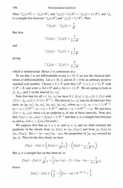
196 Nonstandard analysis
Then ∗ f n(i/4k) = ∗ f k(i/4k), and ∗ f n((i+1)/4k) = ∗ f k((i+1)/4k), and ∗ f kis a straight line between ∗ f k(i/4k) and ∗ f k((i+1)/4k). Thus
|∗ f k(a)−∗ f k(x)| <14k .
But also,
|∗ f k(a)−∗ f n(a)| < 13×4k
and
|∗ f k(x)−∗ f n(x)| <1
3×4k
giving
|∗ f n(a)−∗ f n(x)| <5
3×4k
which is infinitesimal. Hence f is continuous at a.To see that f is not differentiable at any a ∈ [0, 1] we use the classical defi-
nition of differentiability. Let a ∈ [0, 1] and let δ > 0 be an arbitrary positivestandard real number. Choose i, k ∈ N such that i/4k � a � (i + 1)/4k with1/4k < δ , and write x1 for i/4k and x2 for (i + 1)/4k. We are going to look atfk, fk+1 and f on the interval [x1, x2].
Note first that for all x ∈ [x1, x2] we have 0 � fk(x) � fk+1(x) � f (x) with| f (x)− fk+1(x)| � 1/(3×4k+1). The interval [x1, x2] may be divided into fourparts, as [u0, u1], [u1, u2], [u2, u3], [u3, u4], where u0 = x1, u1 = x1 + 1/4k+1,u2 = x1 +2/4k+1, u3 = x1 +3/4k+1, and u2 = x1 +4/4k+1 = x2. We also havef (u) = fk+1(u) when u is an endpoint ui of one of these intervals. Note alsothat f (u2) = fk+1(u2) = fk(u2)+1/4k+1 and that fk is a straight line betweenu0 and u4. Let vi = fk(ui) for each i.
We suppose first that u0 � a � u1 and v0 � v4 and we shall estimate thegradients of the chords from (a, f (a)) to (u2, f (u2)) and from (a, f (a)) to(u4, f (u4)). Set t = (a− u0)/(u4 − u0), the proportion of [u0, u4] covered by[u0, a]. Then for the first chord, we have
f (u2)− f (a) �(
fk(u2)+1
4k+1
)−
(fk(a)+
13×4k+1
).
But fk is a straight line on this interval, so
f (u2)− f (a) � 14k+1 +
12(v0 + v4)− (1− t)v0 − tv4 − 1
3×4k+1
hence
f (u2)− f (a) �(
12− t
)(v4 − v0)+4−(k+1) × 2
3.

12.3 Overspill and applications* 197
The horizontal distance from a to u2 is (1/2− t)/4k and so the gradient of thischord from (a, f (a)) to (u2, f (u2)) is at least
4k(v4 − v0)+16
(12− t
)−1
.
As t � 0 this is at least
4k(v4 − v0)+13.
The gradient of the chord from (a, f (a)) to (u4, f (u4)) is a little easier toestimate. As f (a) � fk(a) it is at most
fk(u4)− fk(a)(1− t)×4−k =
v4 − (1− t)v0 − tv4
(1− t)×4−k =(1− t)(v4 − v0)(1− t)×4−k = 4k(v4 − v0).
Thus the difference between these two gradients is at least 1/3, which is apositive number, independent of k and hence independent of δ . Therefore thefunction f is not differentiable at a since for each δ we can find two chordswithin distance δ of a that differ in gradient by 1/3.
The cases for the other values for a, between u1 and u2, etc., and whenv4 < v0 are treated with a similar calculation of gradients of suitably chosenchords, and are left for the reader to complete and verify. In all cases theconclusion is that f is not differentiable at a, as we require.
Overspill, as we have seen, is an important tool for nonstandard analysis. In itssimplest form it is, however, only a statement about how the standard naturalnumbers sit inside the set of nonstandard natural numbers. As such, it is alsoa tool for understanding number theory, Th(N, 0, 1, +, ×, <) say. Thus inprinciple nonstandard techniques might be applied to number theory, though itturns out that there are (at present) fewer convincing applications in this area.On the other hand, nonstandard models of number theory (or arithmetic, asthey are more usually called) are interesting objects with links and applicationsto many other areas, especially model theory and algebra. For an introductionto models of arithmetic, see Kaye [7].
Exercise 12.19 Show that ∗N contains infinitely many infinite prime numbers.
Exercise 12.20 Suppose that ∗N contains an infinite prime number p such thatp+2 is also prime. Show that this would imply that N contains infinitely manyprimes p such that p+2 is also prime.
The last exercise shows how nonstandard methods may be of use in numbertheory too: proving the existence of a single nonstandard number with a given

198 Nonstandard analysis
property implies the existence of infinitely many standard numbers with thesame property.
Exercise 12.21 Let f : R→R and g: R→R be functions and a ∈ R. Supposef and g are continuous at a and g(a) �= 0. Use nonstandard methods to showf (x)/g(x) is continuous at a (when considered as a function of x). Contrastyour proof with a traditional epsilon-delta proof.
Exercise 12.22 Prove Theorem 12.16 giving the nonstandard characterisationof differentiability.
Exercise 12.23 Prove the chain rule, that if g is differentiable at a ∈R and f isdifferentiable at g(a) ∈ R then the composition f ◦g is differentiable at a withderivative ( f ◦ g)′(a) = f ′(g(a))×g′(a). (Hint: work in a hyperreal structurewith versions ∗ f and ∗g of both f , g.)

References
[1] Martin Aigner and Gunter M. Ziegler, Proofs from The Book. Berlin:Springer-Verlag, third edition, 2004.
[2] George S. Boolos and Richard C. Jeffrey, Computability and Logic. Cambridge:Cambridge University Press, 1989.
[3] Lewis Carroll, Symbolic logic: Part II. Advanced, edited with annotations and anintroduction by William Warren Bartley. New York: Clarkson N. Potter, 1977.
[4] Nigel Cutland, Computability. Cambridge: Cambridge University Press, 1980.[5] Nigel Cutland, editor, Nonstandard Analysis and its Applications, Volume 10 of
London Mathematical Society Student Texts. Cambridge: Cambridge UniversityPress, 1988.
[6] Douglas R. Hofstadter, Godel, Escher, Bach: an Eternal Golden Braid. NewYork: Basic Books, 1979.
[7] Richard Kaye, Models of Peano Arithmetic, Volume 15 of Oxford Logic Guides.Oxford: Oxford University Press, 1991.
[8] Azriel Levy, Basic Set Theory. Berlin: Springer-Verlag, 1979. ReprintedMineola, NY: Dover Publications, 2002.
[9] David Marker, Model Theory: an Introduction, Volume 217 of Graduate Texts inMathematics. New York: Springer-Verlag, 2002.
[10] Thomas L. Saaty and Paul C. Kainen, The Four-Color Problem: Assaults andConquest. New York: Dover Publications, second edition, 1986.
[11] Stephen G. Simpson, editor, Reverse Mathematics 2001, Volume 21 of LectureNotes in Logic. La Jolla, CA: Association for Symbolic Logic, 2005.
[12] Robin Wilson, Four Colors Suffice: How the Map Problem Was Solved.Princeton, NJ: Princeton University Press, 2002.
199

Index
abelian group, 50
aleph, 166ℵ0, 166algorithm, 77, 96alphabet, 35
and (logical connective), ix, 55, 58ant, 3Appel and Haken, 8Archimedean Property, 185, 188arithmetic, models of, 197arity, 118
assumption, 67atom, 107
atomic formula, 78, 119, 138Axiom of Choice, 16, 20, 50, 110, 166axiom scheme, 139axiomatisable theories, 146
back-and-forth, 174Baire’s Theorem, 152, 155Barber Shop Paradox, 76basis, 19, 20bijection, 161, 165binary tree, 5, 12BOOL, 113Boole, George, 61boolean algebra, 56, 57, 100, 113
degenerate, 57dual space of, 110, 111
free, 105improper, 57proper, 103quotient of, 103representation theorem for, 110
Boolean Prime Ideal Theorem, 107, 110, 111boolean ring, 62, 102boolean term, 64, 81, 90, 104
positive, 92
bottom (logical constant), 58
Cantor, Georg, 14, 165, 166cardinal arithmetic, 167, 178cardinality, 161, 165, 166cardinality of
first-order language, 168Carroll, Lewis, 76categoricity, 171, 174category theory, 114chain, 15
chain rule, 198change of variables, 131characteristic function, 62
choice function, 20clopen set, 112closed term, 118, 164closure of a set, 108
co-meagre set, 155
co-nondeterministic computation, 99co-rare set, 154
compact space, 7, 108, 150Compactness Theorem
first-order logic, 145, 150, 160propositional logic, 89
complementation, 57, 58, 60, 61complete theory, 153, 170
completeness of a formal system, 43, 86completeness of the reals, 185Completeness Theorem, viii, 30, 43, 44, 48
arbitrary cardinalities, 169countable version, 164first-order logic, 142, 160, 163propositional logic, 85, 86, 89, 106uncountable version, 167
complexity theory, 96comprehension, axiom scheme of, 139computability, 37, 96computation tree, 9concatenation, 4
conjunction, 91Conjunctive Normal Form (CNF), 92
200

Index 201
connected nodes, 5
connective, 143consistent set, 41, 42, 65, 86constant symbol, 117, 132continuity, 190contradiction, 39Contradiction Rule, 39, 65contrapositive, 59
Cook Wilson, John, 76countable set, 14, 161, 162counter-example, 134cyclic group, 50, 147
decidability, 37, 77Dedekind, Richard, 138Deduction Theorem, 77deductively closed, 152
definable, 160, 175, 176, 187, 189
degenerate algebra, 57
degree, 6
Dense Linear Order (DLO), 173difference equation, 192differential equation, 192differentiation, 185, 191dimension, 20, 172discharged assumption, 67disjunction, 91Disjunctive Normal Form (DNF), 91distributive lattice, 56
Dodgson, Charles, 76domain, 116, 121, 132, 164
empty, 137dual of a propositional connective, 101dual of a quantifier, 136
dual of boolean algebra, Bdual, 110duality, 114
elective element, 62
elimination of quantifiers, 175∧-Elimination, 65∨-Elimination, 65∃-Elimination, 122∀-Elimination, 122→-Elimination, 76, 124¬-Elimination, 65empty function, 161, 166empty string, 24Equality Rules, 122equivalence relation, 49, 129, 162, 167, 178Erdos, Paul, 1Euler method, 192
excluded middle, 75extensionality, axiom of, 139
false (logical constant), 58field, 20filter, 102
maximal, 106
finitely satisfiable, 158
first-order language, 117, 119cardinality of, 168
countable, 163
first-order logic, 116, 133forest, 147formal proof, 25, 29, 39, 122
first-order logic, 122propositional logic, 65
formal system, 24complete, 43
formally real field, 54
formula, 119
closed, 120
foundations of mathematics, 171free boolean algebra, 105
free(X), 105Friedman, Harvey, 10Frankel, Abraham, 16full binary tree, 2
function symbol, 117, 133binary, 118
ternary, 118
unary, 118
Given Statements Rule, 39, 65, 122Given Strings Rule, 24graph, 1, 8, 135, 147
colouring, 8
connected, 147planar, 8
greatest lower bound, 55∧A, 82
group, 147simple, 137, 149torsion, 50, 149
Godel, Kurt, 171
Hausdorff space, 110, 153Henkin axiom, 141
Henkin property, 154
Henkin, Leon, 140Henkinisation, 140, 156, 164, 167, 169Hilbert, David, 171homomorphism, 100
hyperreal number, 182finite, 186
ideal, 20, 101
idempotent element, 62
implication, 58, 59, 61, 76, 77, 124incompleteness of arithmetic, 138inconsistent set, 41, 65
independence, 172infinite paths, 29infinitesimal, 182, 184, 187
202 Index
informal mathematical proof, 70injection, 161, 165, 166, 177internal set or function, 189
∧-Introduction, 65∨-Introduction, 65∃-Introduction, 122∀-Introduction, 122→-Introduction, 76, 124Irreflexivity Rule, 39isolated, 158
isolated type, 157
isomorphism, 101, 171, 174
join (logical connective), 58joke (logical), 182
kernel, 101
Konig’s Lemma, 3, 5, 7, 23
largeness, 102, 155lattice, 55
least upper bound, 55, 186∨A, 82
length, 4
length of the input, 97Lengthening Rule, 24linear order, 11, 15, 46, 49linearly independent, 19logical symbol, 117
logically equivalent, 91
maximal element, 11, 13
maximal filter, 106
maximally consistent set, 142, 149meagre set, 155meet (logical connective), 58metamathematics, 29metaproof, 29metarule, 70, 75metatheorem, 29metric space, 7, 109MIU system, 34model
countable, 164infinite, 169isomorphic, 171
model theory, 160, 170M �σ , 133
module over a ring, 173modus ponens, 76, 124Morley’s Theorem, 172
natural language, 59, 76natural number, 4
infinite, 188nonstandard, 188, 197
negated atomic formula, 78
negation, 39, 57node, 1non-deterministic computation, 9, 98non-distributive lattice, 56non-logical symbol, 117
non-strict partial order, 12
nonstandard analysis, ix, 182, 190not (logical connective), 55, 58nowhere-differentiable function, 194NP, 98NP-complete, 99
number theory, model of, 197numerical analysis, 183
omits p, 158
omitting a type, 156
Omitting Types Theorem, 152, 158Bop, 101open cover, 108
open set, 108, 150opposite, 101optimism, 104or (logical connective), ix, 55, 58order relation, 11ordered abelian group, 50
ordered field, 54, 185overspill, 197overspill principle, 189
pairing function, 163parameter-definable, 189
partial order, 11, 38linearised, 46non-strict, 12strict, 12
partially ordered set, 11path, 3, 5
Peano Existence Theorem, 192Peano, Guiseppe, 138pedantic logician, 133pessimism, 104planar graph, 8
polynomial time, 97
Pope, 126poset, 12, 38
directed, 14
maximal element in, 13positive cone, 54
Post system, 35
power set, 11
predicate logic, 116prenex normal form, 137
preorder, 17, 49pre-positive cone, 54
prime filter, 106
prime ideal, 106
Prime Ideal Theorem, 106
Index 203
problem, 96
product space, 109
projection function, 109, 175proof strategy, 70, 77proof theory, 26propositional letters, 64
propositional logicalgorithm, 95decidability, 77
provability, 24
punctuation symbol, 117
quantifier, 119, 133, 137quantifier elimination, 175quantifier free, 174
quotient, 101, 103
rare set, 155rationals
as ordered set, 173countability of the set of, 18, 163
real numberstandard, 186
realscompleteness of, 185countable model of the theory of, 165structure for set of, 183, 188theory of, 116uncountability of set of, 18
reciprocal, 183Reductio Ad Absurdum (RAA) Rule, 39Reductio Ad Absurdum Rule, 38, 39, 65Reflexivity, 122relation symbol, 117, 133
binary, 119
ternary, 119
unary, 119
representation theorem, 110restriction, 4reverse mathematics, 10right-ordered group, 53
ring, 20, 101ring theory, 100Robinson, Abraham, 182root, 1
SAT, 96
satisfiable, 82, 96
Schroder–Bernstein Theorem, 166, 176scope of a quantifier, 119
Scott’s trick, 166second-order logic, 133, 138semantic deduction, 44semantics, 3, 29, 42, 80, 90, 160sentence, 120, 133sequence, 4
k-sequences, 8
sequential compactness, 7
set theory, 139, 165, 176countable model of, 165
Shortening Rule, 24Simpson, Stephen, 10simultaneous substitution, 122Skolem’s paradox, 165smallness, 102, 155Soundness Theorem, viii, 4, 25, 30
first-order logic, 134logic of posets, 42propositional logic, 84, 105
square-free sequence, 8
stable, 172standard part, 186, 187statement
negative, 45
positive, 45, 47STONE, 113Stone Representation Theorem, 110Stone space, 113
strings, 24structure, viii, 132
cardinality of, 169
countable, 164
L-structure, 132, 133subformula, 119
subgroup, 18subproof, 38, 40, 67subspace topology, 152
substitution, 121valid, 123
Substitution Rule, 122, 127subtraction, 183subtree, 5, 6
support of a type, 157, 158
supremum, 186surjection, 161, 166, 177Symmetry, 122
tableau, 94Tarski’s Fixed Point Lemma, 177Tarski, Alfred, 171, 176TAUT, 96
tautology, 82, 96
term, 118, 122theory, 170
categorical, 171
complete, 170
theory of M, 149
Th(R), 183
tiling problem, 9top (logical constant), 58Top Rule, 65topological space, 108, 149torsion group, 50, 149
torsion-free group, 50, 149
204 Index
total order, 11, 15
totally disconnected space, 111, 150, 153transfer, 182Transitivity, 122transitivity, 38Transitivity Rule, 39transversal, 19
tree, 1, 5, 29binary, 1
describing computations, 9infinite, 3, 5
walk, 3
Trichotomy Theorem, 166, 178true (logical constant), 58truth, 42, 133
in the reals, 183
truth table, 81, 832 (boolean algebra), 57Tychonov’s Theorem, 108, 109type, 158
omitted, 158
realised, 158
ultrafilter, 106, 108, 110uncountable set, 165Unique Readability Theorem, 69upper bound, 15
vacuously, 42
valency, 6
valuation, 80
variable, 35, 117, 119bound, 120
free, 120
renaming, 137substitution of, 122
vector space, 19, 20, 171, 172
well-ordered set, 21, 54
Well-Ordering Principle, 22
Zermelo, Ernst, 16Zermelo–Frankel set theory, 139, 165zero, 4Zorn property, 15
Zorn’s Lemma, 16, 18, 20, 50, 106, 110, 160,168, 176
Zorn, Max, 22


![[S.C. Gupta, V.K. Kapoor] Fundamentals of Mathemat(Bookos.org)](https://static.fdocuments.us/doc/165x107/55cf9c06550346d033a8483b/sc-gupta-vk-kapoor-fundamentals-of-mathematbookosorg.jpg)