The mathematical physics of rainbows and glories - … · The mathematical physics of rainbows and...
137
Physics Reports 356 (2002) 229–365 The mathematical physics of rainbows and glories John A. Adam Department of Mathematics and Statistics, Old Dominion University, Norfolk, VA 23529, USA Received May 2001; editors: J: Eichler; T:F: Gallagher Contents 1. Introduction 231 1.1. Structure and philosophy of the review 231 1.2. The rainbow: elementary physical features 233 1.3. The rainbow: elementary mathematical considerations 243 1.4. Polarization of the rainbow 246 1.5. The physical basis for the divergence problem 250 2. Theoretical foundations 252 2.1. The supernumerary rainbows; a heuristic account of Airy theory 252 2.2. Mie scattering theory 258 3. Glories 260 3.1. The backward glory 260 3.2. Rainbow glories 267 3.3. The forward glory 269 4. Semi-classical and uniform approximation descriptions of scattering 270 5. The complex angular momentum theory: scalar problem 276 5.1. The quantum mechanical connection 276 5.2. The poles of the scattering matrix 280 5.3. The Debye expansion 283 5.4. Geometrical optics r egimes 289 5.5. Saddle points 291 5.6. The glory 297 5.7. Summary of the CAM theory for rainbows and glories 302 5.8. A synopsis: diractive scattering, tunneling eects, shape resonances and Regge trajectories [89] 304 6. The electromagnetic problem 311 6.1. Polarization 311 6.2. Further developments on polarization: Airy theory revisited 314 6.3. Comparison of theories 319 6.4. Non-spherical (non-pendant) drops 326 6.5. Rainbows and glories in atomic, nuclear and particle physics 331 7. The rainbow as a diraction catastrophe 335 8. Summary 343 8.1. The rainbow according to CAM theory 344 Acknowledgements 347 Appendix A. Classical scattering; the scattering cross section 347 A.1. Semi-classical considerations: a pr ecis 351 Appendix B. Airy functions and Fock functions 353 Appendix C. The Watson transform and its modication for the CAM method 354 Appendix D. The Chester–Friedman–Ursell (CFU) method 359 References 360 E-mail address: [email protected] (J.A. Adam). 0370-1573/02/$ - see front matter c 2002 Published by Elsevier Science B.V. PII: S0370-1573(01)00076-X
-
Upload
nguyenkhanh -
Category
Documents
-
view
269 -
download
3
Transcript of The mathematical physics of rainbows and glories - … · The mathematical physics of rainbows and...
Physics Reports 356 (2002) 229–365
The mathematical physics of rainbows and gloriesJohn A. Adam
Department of Mathematics and Statistics, Old Dominion University, Norfolk, VA 23529, USA
Received May 2001; editors: J: Eichler; T:F: Gallagher
Contents
1. Introduction 2311.1. Structure and philosophy of the review 2311.2. The rainbow: elementary physical
features 2331.3. The rainbow: elementary mathematical
considerations 2431.4. Polarization of the rainbow 2461.5. The physical basis for the divergence
problem 2502. Theoretical foundations 252
2.1. The supernumerary rainbows;a heuristic account of Airy theory 252
2.2. Mie scattering theory 2583. Glories 260
3.1. The backward glory 2603.2. Rainbow glories 2673.3. The forward glory 269
4. Semi-classical and uniform approximationdescriptions of scattering 270
5. The complex angular momentum theory:scalar problem 2765.1. The quantum mechanical connection 2765.2. The poles of the scattering matrix 2805.3. The Debye expansion 2835.4. Geometrical optics r7egimes 2895.5. Saddle points 2915.6. The glory 297
5.7. Summary of the CAM theory forrainbows and glories 302
5.8. A synopsis: di9ractive scattering,tunneling e9ects, shape resonancesand Regge trajectories [89] 304
6. The electromagnetic problem 3116.1. Polarization 3116.2. Further developments on polarization:
Airy theory revisited 3146.3. Comparison of theories 3196.4. Non-spherical (non-pendant) drops 3266.5. Rainbows and glories in atomic,
nuclear and particle physics 3317. The rainbow as a di9raction catastrophe 3358. Summary 343
8.1. The rainbow according to CAM theory 344Acknowledgements 347Appendix A. Classical scattering; the scattering
cross section 347A.1. Semi-classical considerations: a pr7ecis 351
Appendix B. Airy functions and Fock functions 353Appendix C. The Watson transform and
its modiAcation for the CAMmethod 354
Appendix D. The Chester–Friedman–Ursell(CFU) method 359
References 360
E-mail address: [email protected] (J.A. Adam).
0370-1573/02/$ - see front matter c© 2002 Published by Elsevier Science B.V.PII: S 0370-1573(01)00076-X
230 J.A. Adam /Physics Reports 356 (2002) 229–365
Abstract
A detailed qualitative summary of the optical rainbow is provided at several complementary levels ofdescription, including geometrical optics (ray theory), the Airy approximation, Mie scattering theory, thecomplex angular momentum (CAM) method, and catastrophe theory. The phenomenon known commonlyas the glory is also discussed from both physical and mathematical points of view: backward glories,rainbow-glories and forward glories. While both rainbows and glories result from scattering of the incidentradiation, the primary rainbow arises from scattering at about 138◦ from the forward direction, whereasthe (backward) glory is associated with scattering very close to the backward direction. In fact, it is amore complex phenomenon physically than the rainbow, involving a variety of di9erent e9ects (includingsurface waves) associated with the scattering droplet. Both sets of optical phenomena—rainbows andglories—have their counterparts in atomic, molecular and nuclear scattering, and these are addressedalso. The conceptual foundations for understanding rainbows, glories and their associated features rangefrom classical geometrical optics, through quantum mechanics (in particular scattering from a square wellpotential; the associated Regge poles and scattering amplitude functions) to di9raction catastrophes. Boththe scalar and the electromagnetic scattering problems are reviewed, the latter providing details about thepolarization of the rainbow that the scalar problem cannot address. The basis for the complex angularmomentum (CAM) theory (used in both types of scattering problem) is a modiAcation of the Watsontransform, developed by Watson in the early part of this century in the study of radio wave di9ractionaround the earth. This modiAed Watson transform enables a valuable and accurate approximation to bemade to the Mie partial-wave series, which while exact, converges very slowly at high frequencies. Thetheory and many applications of the CAM method were developed in a fundamental series of papers byNussenzveig and co-workers (including an important interpretation based on the concept of tunneling), butmany other contributions have been made to the understanding of these beautiful phenomena, includingdescriptions in terms of so-called di9raction catastrophes. The rainbow is a Ane example of an observableevent which may be described at many levels of mathematical sophistication using distinct mathematicalapproaches, and in so doing the connections between several seemingly unrelated areas within physicsbecome evident. c© 2002 Published by Elsevier Science B.V.
PACS: 42.15.−i; 42.25.−p; 42.25.FX; 42.68.Mj
Keywords: Rainbow; Glory; Mie theory; Scattering; Complex angular momentum; Di9raction catastrophe
J.A. Adam /Physics Reports 356 (2002) 229–365 231
Like the appearance of a rainbow in the clouds on a rainy day, so was the radiance aroundhim. This was the appearance of the likeness of the glory of the Lord...The Book of Ezekiel, chapter 1, verse 28 (New International Version of the Bible).
1. Introduction
1.1. Structure and philosophy of the review
The rainbow is at one and the same time one of the most beautiful visual displays in natureand, in a sense, an intangible phenomenon. It is illusory in that it is not of course a solid arch,but like mirages, it is nonetheless real. It can be seen and photographed, and described as aphenomenon of mathematical physics, but it cannot be located at a speciAc place, only in aparticular direction. What then is a rainbow? Since many levels of description will be encoun-tered along the way, the answers to this question will take us on a rather long but fascinatingjourney in the footsteps of those who have made signiAcant contributions to the subject of “lightscattering by small particles”. Let us Arst ‘listen’ to what others have written about rainbowsand the mathematical tools with which to understand them.
“Rainbows have long been a source of inspiration both for those who would prefer to treatthem impressionistically or mathematically. The attraction to this phenomenon of D7escartes,Newton, and Young, among others, has resulted in the formulation and testing of some ofthe most fundamental principles of mathematical physics.” K. Sassen [1].
“The rainbow is a bridge between two cultures: poets and scientists alike have long beenchallenged to describe it: : : Some of the most powerful tools of mathematical physicswere devised explicitly to deal with the problem of the rainbow and with closely relatedproblems. Indeed, the rainbow has served as a touchstone for testing theories of optics.With the more successful of those theories it is now possible to describe the rainbowmathematically, that is, to predict the distribution of light in the sky. The same methods canalso be applied to related phenomena, such as the bright ring of color called the glory, andeven to other kinds of rainbows, such as atomic and nuclear ones.” H.M. Nussenzveig [2].
“Probably no mathematical structure is richer, in terms of the variety of physical situationsto which it can be applied, than the equations and techniques that constitute wave theory.Eigenvalues and eigenfunctions, Hilbert spaces and abstract quantum mechanics, numericalFourier analysis, the wave equations of Helmholtz (optics, sound, radio), SchrRodinger (elec-trons in matter), Dirac (fast electrons) and Klein–Gordon (mesons), variational methods,scattering theory, asymptotic evaluation of integrals (ship waves, tidal waves, radio wavesaround the earth, di9raction of light)—examples such as these jostle together to prove theproposition.” M.V. Berry [3].
The three quotations above provide a succinct yet comprehensive survey of the topic addressedin this review: the mathematical physics of rainbows and glories. An attempt has been made toprovide complementary levels of description of the rainbow and related phenomena; this mirrors
232 J.A. Adam /Physics Reports 356 (2002) 229–365
to some extent the historical development of the subject, but at a deeper level it addresses thefact that, in order to understand a given phenomenon as fully as possible, it is necessary tostudy it at as many complementary levels of description as possible. In the present context, thismeans both descriptive and mathematical accounts of the rainbow and related phenomena, thelatter account forming the basis of the paper: it is subdivided into the various approaches andlevels of mathematical sophistication that have characterized the subject from the investigationsof D7escartes down to the present era.
There are several classic books and important papers that have been drawn on frequentlythroughout this paper: the book by Greenler on rainbows, halos and glories [4] has provedinvaluable for the descriptive physics in this introduction; the article by Nussenzveig [2] fromwhich the second quotation is taken is an excellent introduction to both the physics and thequalitative description of the various mathematical theories that exist for the rainbow. The twopapers [5,6] by the same author constitute a major thread running throughout this article, butparticularly so in Section 5 (complex angular momentum theory). Van de Hulst’s book on lightscattering by small particles [7] is a classic in the Aeld, and for that reason is often cited, bothin this article and in many of the references. Indeed, to quote from Section 13:2 in that book
“The rainbow is one of the most beautiful phenomena in nature. It has inspired art andmythology in all people, and it has been a pleasure and challenge to the mathematicalphysicists of four centuries. A person browsing through the old literature receives theimpression that a certain a9ection for this problem pervades even the driest computations.”
The very next sentence in the above citation is most Sa propos, since it also accurately reTectsthis author’s hopes for the present article
“The writer hopes that the following report, though it has to be concise and must leaveout most of the history, will to some extent demonstrate this mathematical beauty.”
Another important book, less comprehensive and mathematically complete than [7], but nonethe-less extremely valuable from both physical and mathematical viewpoints, is that by Tricker onmeteorological optics [8]. The book by Bohren and Hu9man [9] provides a great deal of in-formation on the absorption and scattering of light by small particles and diverse applications,with many references. At the time of writing, the most comprehensive and up-to-date book ondi9raction e9ects in semi-classical scattering theory and its applications is that by Nussenzveig[10]. It is a seminal work, and incorporates many of the topics addressed here (amongst others),and should be consulted by anyone wishing to study the subject from an expert in the Aeld.
No attempt is made here to discuss the historical development of the theory of the rainbowexcept insofar as it is germane to the context; that topic is superbly treated in the book by Boyer[11]. A noteworthy and somewhat technical account of more recent historical developments canbe found in the review article by Logan [12]. It is a survey of early studies in the scatteringof plane waves by a sphere. This is extremely important and interesting from a historicalperspective: Logan provides 103 references, and in so doing notes that the literature appears tobe characterized by writers who, it seems, failed to recognize the signiAcance of the contributionsmade by their predecessors and contemporaries. There are several instances of the “rediscoveryof the wheel” (so to speak), and the author has performed a valuable task in identifying the“lost” contributions to the subject.
J.A. Adam /Physics Reports 356 (2002) 229–365 233
In the rest of this introduction, elementary physical and mathematical descriptions (e.g. geo-metrical optics) of the rainbow are provided. Section 2 addresses the capacity of Airy’s theoryto account for, among other things, the primary bow and its associated supernumeraries. InSection 3 glories (backward, forward and rainbow-modiAed) are described; Section 4 addressesthe semiclassical description of atomic, molecular and nuclear rainbows and glories, as wellas di9ractive=tunneling e9ects in these areas and in particle physics. Section 5 is devoted to asummary of the complex angular momentum (CAM) theory for the scalar scattering problem;a fascinating and very powerful tool for understanding many of the subtleties of wave scat-tering by both impenetrable and transparent (or even absorbing) spheres. It is appropriate toinclude the topic of the glory again in this section, because much of the CAM theory devel-oped by Nussenzveig addressed both rainbows and glories. In Section 6 further developmentsare discussed, including the full electromagnetic problem (Mie scattering theory), polarization,alternative models, the e9ects of non-spherical droplets, and a comparison of theories. A briefaccount of rainbows and glories in atomic, molecular and nuclear scattering is also provided.Section 7 contains an account of the relevant aspects of ‘di9raction catastrophe’ scattering tothe problem at hand. The summary in Section 8 precedes four appendices: Appendix A sum-marizes aspects of classical scattering relevant to the present article, and previews rainbow andglory scattering, forward peaking and orbiting, all of which reappear in a semiclassical context.Appendix B provides brief details of the Airy and Fock functions referred to in the article.Appendix C contains a brief account of the Watson transform and its modiAcation to becomethe basis of the CAM theory discussed earlier, while Appendix D is a brief summary of theChester–Friedmann–Ursell (CFU) method.
1.2. The rainbow: elementary physical features
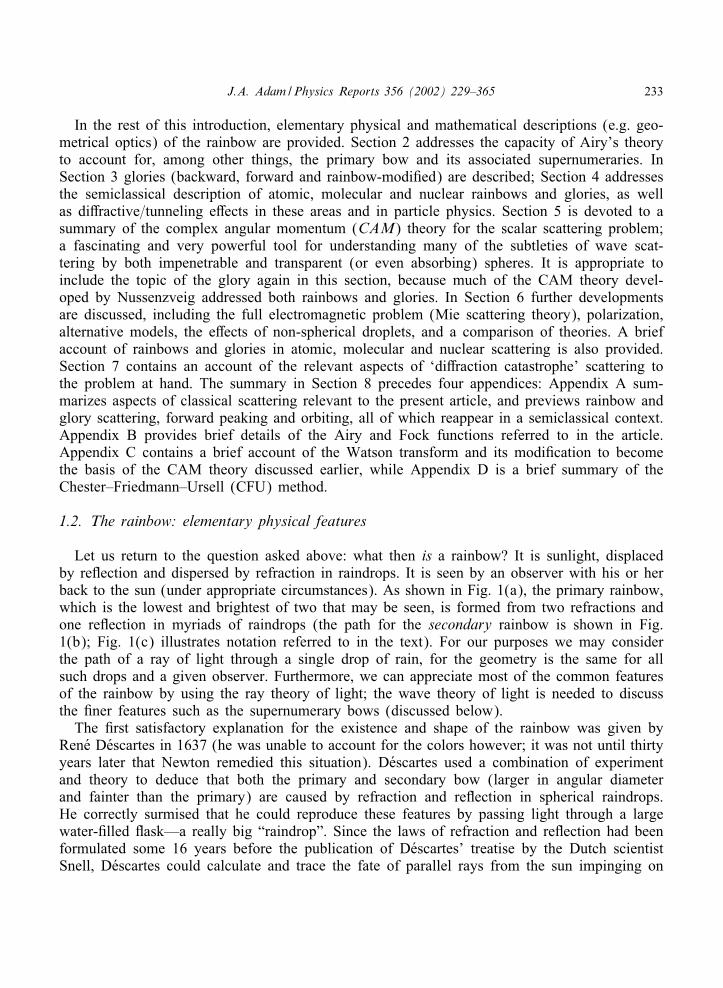
Let us return to the question asked above: what then is a rainbow? It is sunlight, displacedby reTection and dispersed by refraction in raindrops. It is seen by an observer with his or herback to the sun (under appropriate circumstances). As shown in Fig. 1(a), the primary rainbow,which is the lowest and brightest of two that may be seen, is formed from two refractions andone reTection in myriads of raindrops (the path for the secondary rainbow is shown in Fig.1(b); Fig. 1(c) illustrates notation referred to in the text). For our purposes we may considerthe path of a ray of light through a single drop of rain, for the geometry is the same for allsuch drops and a given observer. Furthermore, we can appreciate most of the common featuresof the rainbow by using the ray theory of light; the wave theory of light is needed to discussthe Aner features such as the supernumerary bows (discussed below).
The Arst satisfactory explanation for the existence and shape of the rainbow was given byRen7e D7escartes in 1637 (he was unable to account for the colors however; it was not until thirtyyears later that Newton remedied this situation). D7escartes used a combination of experimentand theory to deduce that both the primary and secondary bow (larger in angular diameterand fainter than the primary) are caused by refraction and reTection in spherical raindrops.He correctly surmised that he could reproduce these features by passing light through a largewater-Alled Task—a really big “raindrop”. Since the laws of refraction and reTection had beenformulated some 16 years before the publication of D7escartes’ treatise by the Dutch scientistSnell, D7escartes could calculate and trace the fate of parallel rays from the sun impinging on
234 J.A. Adam /Physics Reports 356 (2002) 229–365
Fig. 1. (a) the basic geometry of ray paths in a spherical raindrop for the primary rainbow; O is the center of thedrop, and i, r, respectively, are the angles of incidence and refraction. The incident and exiting ‘wavefronts’ A′A′′and B′B′′ are also shown (refer to Section 2.1), (b) the corresponding geometry for the formation of the secondaryrainbow, (c) the geometry of an incident ray (1) showing the externally reTected ray (1′), the transmitted ray (2)and externally refracted ray (2′), etc. All externally transmitted rays are denoted by primed numbers.
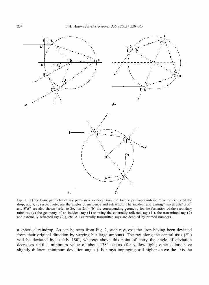
a spherical raindrop. As can be seen from Fig. 2, such rays exit the drop having been deviatedfrom their original direction by varying but large amounts. The ray along the central axis (#1)will be deviated by exactly 180◦, whereas above this point of entry the angle of deviationdecreases until a minimum value of about 138◦ occurs (for yellow light; other colors haveslightly di9erent minimum deviation angles). For rays impinging still higher above the axis the
J.A. Adam /Physics Reports 356 (2002) 229–365 235
Fig. 2. The paths of several rays through a spherical raindrop illustrating the di9erences in total deTection anglefor di9erent angles of incidence (or equivalently, di9erent impact parameters). The ray #7 is called the rainbow rayand this ray deAnes the minimum angle of deTection in the primary rainbow. (Redrawn from [4].)
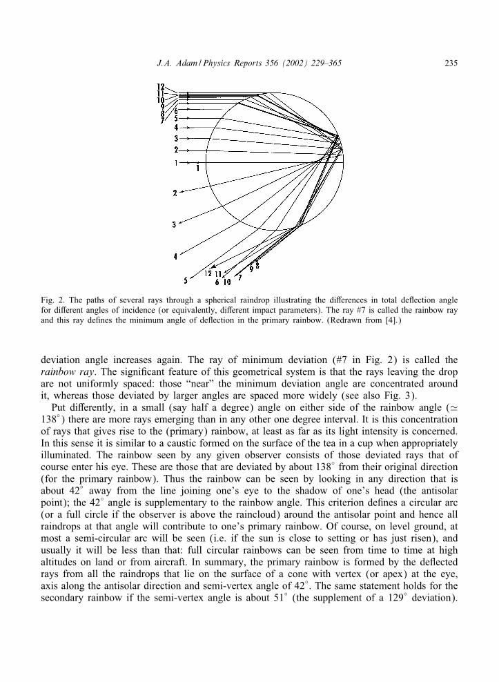
deviation angle increases again. The ray of minimum deviation (#7 in Fig. 2) is called therainbow ray. The signiAcant feature of this geometrical system is that the rays leaving the dropare not uniformly spaced: those “near” the minimum deviation angle are concentrated aroundit, whereas those deviated by larger angles are spaced more widely (see also Fig. 3).
Put di9erently, in a small (say half a degree) angle on either side of the rainbow angle (�138◦) there are more rays emerging than in any other one degree interval. It is this concentrationof rays that gives rise to the (primary) rainbow, at least as far as its light intensity is concerned.In this sense it is similar to a caustic formed on the surface of the tea in a cup when appropriatelyilluminated. The rainbow seen by any given observer consists of those deviated rays that ofcourse enter his eye. These are those that are deviated by about 138◦ from their original direction(for the primary rainbow). Thus the rainbow can be seen by looking in any direction that isabout 42◦ away from the line joining one’s eye to the shadow of one’s head (the antisolarpoint); the 42◦ angle is supplementary to the rainbow angle. This criterion deAnes a circular arc(or a full circle if the observer is above the raincloud) around the antisolar point and hence allraindrops at that angle will contribute to one’s primary rainbow. Of course, on level ground, atmost a semi-circular arc will be seen (i.e. if the sun is close to setting or has just risen), andusually it will be less than that: full circular rainbows can be seen from time to time at highaltitudes on land or from aircraft. In summary, the primary rainbow is formed by the deTectedrays from all the raindrops that lie on the surface of a cone with vertex (or apex) at the eye,axis along the antisolar direction and semi-vertex angle of 42◦. The same statement holds for thesecondary rainbow if the semi-vertex angle is about 51◦ (the supplement of a 129◦ deviation).
236 J.A. Adam /Physics Reports 356 (2002) 229–365
Fig. 3. A more detailed version of Fig. 2 showing the “Airy wavefront” (which is perpendicular to all rays of class3’ in Fig. 1(c)). Also shown, following Nussenzveig [2] are the caustics (one real, one imaginary) of these rays;these are envelopes of the ray system. (Redrawn from [2].)
These cones will be di9erent for each observer, so each person has his or her own personalrainbow.
Up to this point, we have been describing a generic, colorless type of rainbow. Blue and violetlight get refracted more than red light: the actual amount depends on the index of refraction ofthe raindrop, and the calculations thereof vary slightly in the literature because the wavelengthschosen for “red” and “violet” may di9er slightly. Thus, for a wavelength of 6563 WA (Angstromunits; 1 WA=10−10 m) the cone semi-angle is about 42:3◦, whereas for violet light of 4047 WAwavelength, the cone semi-angle is about 40:6◦, about a 1:7◦ angular spread for the primarybow. A similar spread (dispersion) occurs for the secondary bow, but the additional reTectionreverses the sequence of colors, so the red in this bow is on the inside of the arc.
In principle more than two internal reTections may take place inside each raindrop, sohigher-order rainbows (tertiary, quaternary, etc.) are possible. It is possible to derive the angularsize of such a rainbow after any given number of reTections (Newton was the Arst to do this).Newton’s contemporary, Edmund Halley found that the third rainbow arc should appear as acircle of angular radius about 40◦ around the sun itself. The fact that the sky background isso bright in this vicinity, coupled with the intrinsic faintness of the bow itself would makesuch a bow almost impossible, if not impossible to see (but see [13]). Jearl Walker has useda laser beam to illuminate a single drop of water and traced rainbows up to the 13th order,their positions agreeing closely with predictions. Others have traced 19 rainbows under similarlaboratory conditions [14].
J.A. Adam /Physics Reports 356 (2002) 229–365 237
The sky below the primary rainbow is often noticeably brighter than the sky outside it; in-deed the region between the primary and secondary bow is called Alexander’s dark band (afterAlexander of Aphrodisias who studied it in connection with Aristotle’s (incorrect) theory of therainbow). Raindrops scatter incident sunlight in essentially all directions, but as we have seen,the rainbow is a consequence of a “caustic” or concentration of such scattered light in a particu-lar region of the sky. The reason the inside of the primary bow (i.e. inside the cone) is bright isthat all the raindrops in the interior of the cone reTect light to the eye also, (some occurring fromdirect reTections at their surfaces) but it is not as intense as the rainbow light, and it is composedof many colors intermixed. Similarly, outside the secondary bow a similar (but less obvious)e9ect occurs (see Figs. 4:3(b) and 4:7 in [15]). Much of the scattered light then, comes fromraindrops through which sunlight is refracted and reTected: these rays do not emerge betweenthe 42◦ and 51◦ angle. This dark angular band is not completely dark, of course, because the sur-faces of raindrops reTect light into it; the reduction of intensity, however, is certainly noticeable.
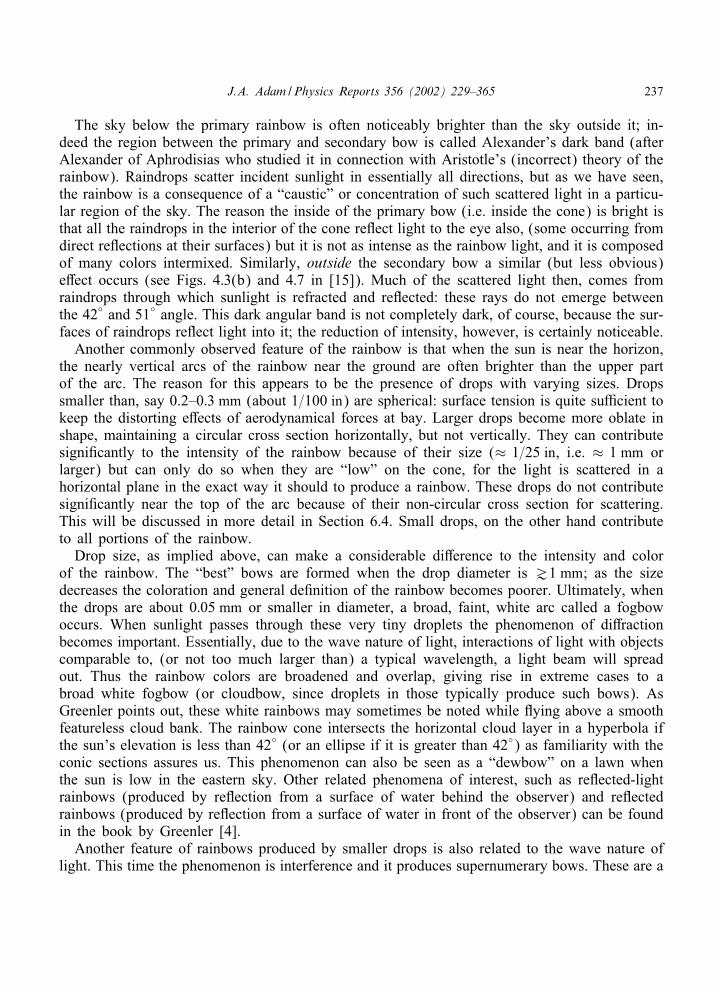
Another commonly observed feature of the rainbow is that when the sun is near the horizon,the nearly vertical arcs of the rainbow near the ground are often brighter than the upper partof the arc. The reason for this appears to be the presence of drops with varying sizes. Dropssmaller than, say 0.2–0:3 mm (about 1=100 in) are spherical: surface tension is quite suYcient tokeep the distorting e9ects of aerodynamical forces at bay. Larger drops become more oblate inshape, maintaining a circular cross section horizontally, but not vertically. They can contributesigniAcantly to the intensity of the rainbow because of their size (≈ 1=25 in, i.e. ≈ 1 mm orlarger) but can only do so when they are “low” on the cone, for the light is scattered in ahorizontal plane in the exact way it should to produce a rainbow. These drops do not contributesigniAcantly near the top of the arc because of their non-circular cross section for scattering.This will be discussed in more detail in Section 6.4. Small drops, on the other hand contributeto all portions of the rainbow.
Drop size, as implied above, can make a considerable di9erence to the intensity and colorof the rainbow. The “best” bows are formed when the drop diameter is &1 mm; as the sizedecreases the coloration and general deAnition of the rainbow becomes poorer. Ultimately, whenthe drops are about 0:05 mm or smaller in diameter, a broad, faint, white arc called a fogbowoccurs. When sunlight passes through these very tiny droplets the phenomenon of di9ractionbecomes important. Essentially, due to the wave nature of light, interactions of light with objectscomparable to, (or not too much larger than) a typical wavelength, a light beam will spreadout. Thus the rainbow colors are broadened and overlap, giving rise in extreme cases to abroad white fogbow (or cloudbow, since droplets in those typically produce such bows). AsGreenler points out, these white rainbows may sometimes be noted while Tying above a smoothfeatureless cloud bank. The rainbow cone intersects the horizontal cloud layer in a hyperbola ifthe sun’s elevation is less than 42◦ (or an ellipse if it is greater than 42◦) as familiarity with theconic sections assures us. This phenomenon can also be seen as a “dewbow” on a lawn whenthe sun is low in the eastern sky. Other related phenomena of interest, such as reTected-lightrainbows (produced by reTection from a surface of water behind the observer) and reTectedrainbows (produced by reTection from a surface of water in front of the observer) can be foundin the book by Greenler [4].
Another feature of rainbows produced by smaller drops is also related to the wave nature oflight. This time the phenomenon is interference and it produces supernumerary bows. These are a
238 J.A. Adam /Physics Reports 356 (2002) 229–365
series of faint pink or green arcs (2–4 perhaps) just beneath the top of the primary bow, or muchmore rarely, just above the top of the secondary bow. They rarely extend around the fully visiblearc, for reasons that are again related to drop size. Two rays that enter the drop on either side ofthe rainbow ray (the ray of minimum deviation) may exit the drop in parallel paths; this certainlywill happen for appropriately incident rays. By considering the wavefronts (perpendicular to therays), it is clear that if the incident waves are in phase (i.e. crests and troughs aligned withcrests and troughs) the emerging rays will not be in phase, in general. Inside the drop they travelalong paths of di9erent length. Depending on whether this path di9erence is an integral numberof wavelengths or an odd integral number of half-wavelengths, these waves will reinforce eachother (constructive interference) or annihilate each other (destructive interference). Obviouslypartially constructive=destructive interference can occur if the path di9erence does not meetthe above criteria exactly. Where waves reinforce one another, the intensity of light will beenhanced; conversely, where they annihilate one another the intensity will be reduced. Sincethese beams of light will exit the raindrop at a smaller angle to the axis than the D7escartes ray,the net e9ect for an observer looking in this general direction will be a series of light and darkbands just inside the primary bow.
The angular spacing of these bands depends on the size of the droplets producing them (seeFig. 4). The width of individual bands and the spacing between them decreases as the drops getlarger. If drops of many di9erent sizes are present, these supernumerary arcs tend to overlapsomewhat and smear out what would have been obvious interference bands for droplets ofuniform size. This is why these pale blue or pink or green bands are then most noticeable nearthe top of the rainbow: it is the smaller drops that contribute to this part of the bow, and thesemay represent a rather narrow range of sizes. Nearer the horizon a wide range of drop sizecontributes to the bow, but as we have seen, at the same time it tends to blur the interferencebands.
There are many complementary levels of mathematical techniques with which one can de-scribe the formation and structure of the rainbow. In this section we examine the broad featuresusing only elementary calculus; one account of the basic mathematics is described in [16] (anda useful graphical account is provided in [17]); a thorough treatment of the related physicsof multiple rainbows may be found in the article by Walker [14]. More mathematical detailsare found in two classical works, one by Humphreys [18] and the other by Tricker [8]. In[16] the description of the location and color of the rainbow is approached as an exercise inmathematical modeling: the laws of reTection and refraction are stated along with the underly-ing assumptions about the deviation of sunlight by a raindrop (e.g. the sphericity of the drop;parallel light “rays” from the sun, neither of which are strictly true, of course; the raindropbeing Axed during the scattering process, amongst other ‘axioms’). At this elementary level ofdescription involving geometrical optics, dispersion, geometry, trigonometry and calculus of asingle variable, a reasonably satisfactory “explanation” of the main features of the rainbow ispossible. Incorporation of wave interference and di9raction, amongst other things, is necessaryto take the description further, and as we shall see, this can lead to very sophisticated modelsindeed.
A most fascinating aspect of the topic at hand is the fact that rainbows and glories can also beproduced in atomic, molecular and nuclear scattering experiments, thus illustrating at a profoundlevel the wave=particle duality of matter and radiation. Rays in geometrical optics become
J.A. Adam /Physics Reports 356 (2002) 229–365 239
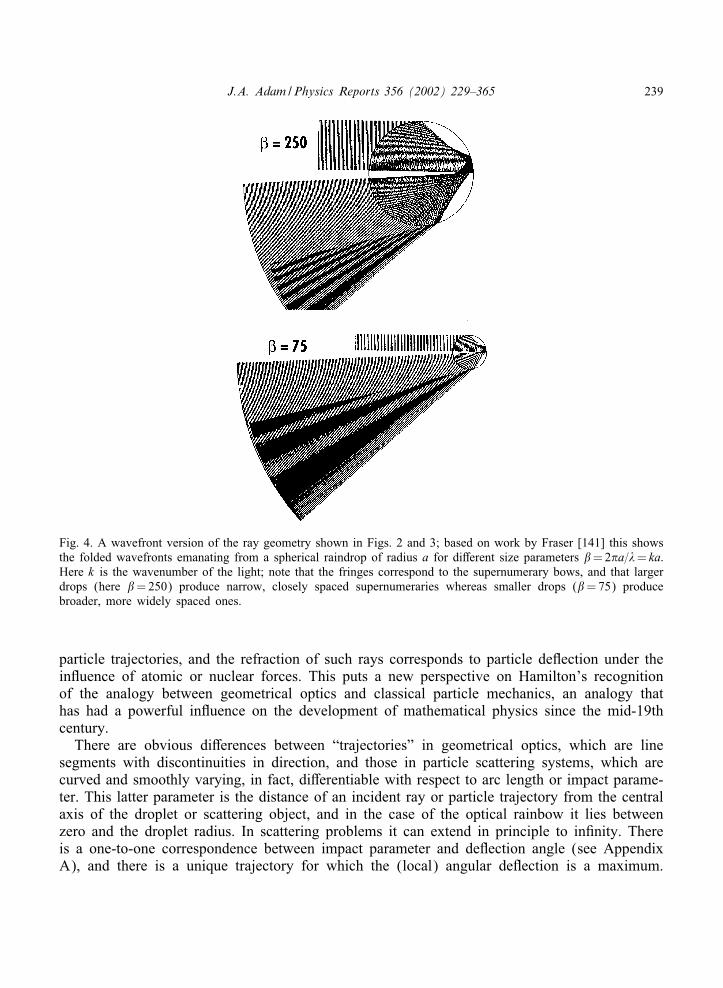
Fig. 4. A wavefront version of the ray geometry shown in Figs. 2 and 3; based on work by Fraser [141] this showsthe folded wavefronts emanating from a spherical raindrop of radius a for di9erent size parameters =2�a=�= ka:Here k is the wavenumber of the light; note that the fringes correspond to the supernumerary bows, and that largerdrops (here =250) produce narrow, closely spaced supernumeraries whereas smaller drops (=75) producebroader, more widely spaced ones.
particle trajectories, and the refraction of such rays corresponds to particle deTection under theinTuence of atomic or nuclear forces. This puts a new perspective on Hamilton’s recognitionof the analogy between geometrical optics and classical particle mechanics, an analogy thathas had a powerful inTuence on the development of mathematical physics since the mid-19thcentury.
There are obvious di9erences between “trajectories” in geometrical optics, which are linesegments with discontinuities in direction, and those in particle scattering systems, which arecurved and smoothly varying, in fact, di9erentiable with respect to arc length or impact parame-ter. This latter parameter is the distance of an incident ray or particle trajectory from the centralaxis of the droplet or scattering object, and in the case of the optical rainbow it lies betweenzero and the droplet radius. In scattering problems it can extend in principle to inAnity. Thereis a one-to-one correspondence between impact parameter and deTection angle (see AppendixA), and there is a unique trajectory for which the (local) angular deTection is a maximum.
240 J.A. Adam /Physics Reports 356 (2002) 229–365
By analogy this is the “rainbow angle” for the interaction because a concentration of scatteredparticles arises near this angle. However, the analogy extends much further than this, for aswill be noted in Section 4, Ford and Wheeler [19] carried out a wave–mechanical analysis ofatomic and nuclear rainbows, showing that interference between trajectories emerging in thesame direction gives rise to supernumerary bows (peaks in intensity). Furthermore, it has beenpossible to formulate an analogue of Airy’s theory (Section 2) for particle scattering. In 1964,Hundhausen and Pauly [20] made the Arst observations of an atomic rainbow with an exper-iment in which sodium atoms were scattered by mercury atoms. The “primary” bow (there isno secondary) and two supernumeraries were detected; subsequent experiments have revealedstructure at yet Aner scales. Just as careful observations of optical rainbows yield informationon the scatterering centers—the raindrops, the refractive index, etc., so too do experiments suchas these. The atomic (and for that matter, molecular and nuclear) rainbow angle depends onthe strength of the interaction, speciAcally the attractive part, and the range of the interactionin turn determines the positions of the supernumerary bows. This topic will be discussed atgreater length in Section 6.5.
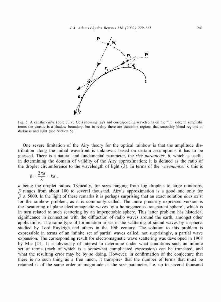
Returning to the optical rainbow, it is important to note that the theories of D7escartes, Newtonand even Young’s interference theory all predicted an abrupt transition between regions ofillumination and shadow (as at the edges of Alexander’s dark band when rays only givingrise to the primary and secondary bows are considered). In the wave theory of light suchsharp boundaries are softened by di9raction—and this should have been Young’s conclusion,incidentally, for his was a wave theory [2]. In 1835, Potter showed that the rainbow ray canbe interpreted as a caustic, i.e. the envelope of the system of rays comprising the rainbow. Theword caustic means “burning curve”, and caustics are associated with regions of high intensityillumination (as we shall below, geometrical optics predicts an inAnite intensity there). Whenthe emerging rays comprising the rainbow are extended backward through the drop, anothercaustic (a virtual one) is formed, associated with the real caustic on the illuminated side of thedrop. Typically, the number of rays di9ers by two on each side of a caustic at any given point,so the rainbow problem is essentially that of determining the intensity of (scattered) light in theneighborhood of a caustic (see Fig. 3, and also Fig. 5). This was exactly what Airy attemptedto do several years later in 1838 [21]. The principle behind Airy’s approach was establishedby Huygens in the 17th century: Huygens’ principle regards every point of a wavefront as asecondary source of waves, which in turn deAnes a new wavefront and hence determines thesubsequent propagation of the wave. Airy reasoned that if one knew the amplitude distributionof the waves along any complete wavefront in a raindrop, the distribution at any other pointcould be determined by Huygens’ principle. However, the problem is to And the initial amplitudedistribution. Airy chose as his starting point a wavefront surface inside the raindrop, the surfacebeing orthogonal to all the rays which comprise the primary bow; this surface has a pointof inTection wherever it intersects the ray of minimum deviation—the rainbow ray. Using thestandard assumptions of di9raction theory, he formulated the local intensity of scattered lightin terms of a “rainbow integral”, subsequently renamed the Airy integral in his honor (it isrelated to the now familiar Airy function; see Appendix B. Note that there is another so-calledAiry function in optics which has nothing to do with this phenomenon [22]). Qualitatively, theintensity distribution so produced is similar to that associated with the shadow of a straightedge, particularly when external reTection is included (see [23, Chapter 8]).
J.A. Adam /Physics Reports 356 (2002) 229–365 241
Fig. 5. A caustic curve (bold curve CC) showing rays and corresponding wavefronts on the “lit” side; in simplisticterms the caustic is a shadow boundary, but in reality there are transition regions that smoothly blend regions ofdarkness and light (see Section 5).
One severe limitation of the Airy theory for the optical rainbow is that the amplitude dis-tribution along the initial wavefront is unknown: based on certain assumptions it has to beguessed. There is a natural and fundamental parameter, the size parameter, ; which is usefulin determining the domain of validity of the Airy approximation; it is deAned as the ratio ofthe droplet circumference to the wavelength of light (�). In terms of the wavenumber k this is
=2�a�
= ka ;
a being the droplet radius. Typically, for sizes ranging from fog droplets to large raindrops, ranges from about 100 to several thousand. Airy’s approximation is a good one only for& 5000: In the light of these remarks it is perhaps surprising that an exact solution does existfor the rainbow problem, as it is commonly called. The more precisely expressed version isthe ‘scattering of plane electromagnetic waves by a homogeneous transparent sphere’, which isin turn related to such scattering by an impenetrable sphere. This latter problem has historicalsigniAcance in connection with the di9raction of radio waves around the earth, amongst otherapplications. The same type of formulation arises in the scattering of sound waves by a sphere,studied by Lord Rayleigh and others in the 19th century. The solution to this problem isexpressible in terms of an inAnite set of partial waves called, not surprisingly, a partial waveexpansion. The corresponding result for electromagnetic wave scattering was developed in 1908by Mie [24]. It is obviously of interest to determine under what conditions such an inAniteset of terms (each of which is a somewhat complicated expression) can be truncated, andwhat the resulting error may be by so doing. However, in conArmation of the conjecture thatthere is no such thing as a free lunch, it transpires that the number of terms that must beretained is of the same order of magnitude as the size parameter, i.e. up to several thousand
242 J.A. Adam /Physics Reports 356 (2002) 229–365
for the rainbow problem! The “why is the sky blue?” scattering problem, on the other hand—Rayleigh scattering—requires only one term because the scatterers are molecules which aremuch smaller than a wavelength, so the simplest truncation—retaining only the Arst term—isperfectly adequate. Although in principle the rainbow problem can be “solved” with enoughcomputer time and resources, numerical solutions by themselves (as Nussenzveig points out)o9er little or no insight into the physics of the phenomenon.
Fortunately help was at hand. The now-famous Watson transformation, developed by Watson[25] is a method for transforming the slowly converging partial-wave series into a rapidly con-vergent expression involving an integral in the complex angular-momentum plane (see AppendixC). But why angular momentum? Although they possess zero rest mass, photons have energyE = hc=� and momentum E=c= h=� where h is Planck’s constant and c is the speed of light invacuo. Thus, for a non-zero impact parameter bi, a photon will carry an angular momentumbih=�, (which can in fact assume only certain discrete values). Each of these discrete valuescan be identiAed with a term in the partial wave series expansion. Furthermore, as the photonundergoes repeated internal reTections, it can be thought of as orbiting the center of the rain-drop. Why complex angular momentum? This allows some powerful mathematical techniquesto “redistribute” the contributions to the partial wave series into a few points in the complexplane—speciAcally poles (called Regge poles in elementary particle physics) and saddle points.Such a decomposition means that instead of identifying angular momentum with certain discretereal numbers, it is now permitted to move continuously through complex values. However, de-spite this modiAcation, the poles and saddle points have profound physical interpretations in therainbow problem; (this is known in other contexts: in many wave propagation problems polesand branch points of Green’s functions in the complex plane can be identiAed with trappedand freely propagating waves, respectively, or in terms of discrete and continuous spectra ofcertain Sturm–Liouville operators (see e.g. [26–28] and references therein). A thoughtful andsomewhat philosophical response to the question ‘why complex angular momentum?’ appearsin a quotation at the very end of this review (Section 8).
Mathematical details will be provided later in Section 5, but for now it will suYce to pointout that since real saddle points correspond to ordinary rays of light, we might expect com-plex saddle points to correspond in some sense to complex rays (whatever that might mean).Again, in problems of wave propagation, imaginary components can often be identiAed withthe damping of some quantity—usually the amplitude—in space or time. An elementary butperfect example of this can be found in the phenomenon of (critical) total internal reTection oflight at a glass=air or water=air boundary: the “refracted” ray is in e9ect a surface wave, prop-agating along the interface with an amplitude which diminishes exponentially away from thatinterface. Such waves are sometimes identiAed as “evanescent”, and are common in many othernon-quantum contexts [26]. Typically, the intensity is negligible on the order of a wavelengthaway from the interface; this deAnes a type of “skin depth”. Quantum-mechanical tunnelinghas a similar mathematical description, and, directly related to the rainbow problem, complexrays can appear on the shadow side of a caustic, where they represent the damped amplitudeof di9racted light.
In the light of this (no pun intended) it is interesting to note that there is another type ofsurface wave: this one is associated with the Regge pole contributions to the partial-waveexpansion. Such waves are initiated when the impact parameter is the drop diameter, i.e.
J.A. Adam /Physics Reports 356 (2002) 229–365 243
the incident ray is tangential to the sphere. These waves are damped in the direction of in-creasing arc-length along the surface, i.e. tangentially, (as opposed to radially, in the case of anevanescent wave) because at each point along its circumferential path the wave penetrates thespherical drop at the critical angle for total internal reTection, in a reversal of the normal event.Subsequently it will re-emerge as a surface wave after taking one or more of these shortcuts. In[2] Nussenzveig points out that this “pinwheel” path for light rays was considered by Kepler in1584 (see [11,29]) as a possible explanation for the rainbow, but he did not pursue it becausehe could not reproduce the correct rainbow angle.
It is important to note that the Watson transformation was originally introduced in con-nection with the di9raction of radio waves around the earth [25], alluded to above. In 1937,Van der Pol and Bremmer [30,31] applied it to the rainbow problem, but, notwithstanding aclaim by Sommerfeld that the problem had now been brought to a beautiful conclusion [32],they were able only to establish that the Airy approximation could be recovered as a limitingcase. (Their papers contain some very beautiful and detailed mathematics, however, and aresigniAcant contributions nonetheless.) In some profound and highly technical papers Nussen-zveig subsequently developed a modiAcation of the transformation [33,5,6] (a valuable summaryof his work up to that point may be found in [34]; references to more recent work will bemade throughout the review) and was able to bring the problem to the desired conclusion us-ing some extremely sophisticated mathematical techniques without losing sight of the physicalimplications.
In the simplest Cartesian terms, on the illuminated side of the rainbow (in a limiting sense)there are two rays of light emerging in parallel directions: at the rainbow angle they coalesceinto the ray of minimum deTection, and on the shadow side, according to geometrical optics,they vanish (this is actually a good deAnition of a caustic curve or surface; refer again to Fig. 5).From the above general discussion of real and complex rays it should not be surprising that, inthe complex angular momentum plane, a rainbow in mathematical terms is the collision of tworeal saddle points. But this is not all: this collision does not result in the mutual annihilation ofthese saddle points; instead a single complex saddle point is born, corresponding to a complexray on the shadow side of the caustic curve. This is directly associated with the di9racted lightin Alexander’s dark band.
1.3. The rainbow: elementary mathematical considerations
As already noted, the primary rainbow is seen in the direction corresponding to the mostdense clustering of rays leaving the drop after a single internal reTection. Correspondinglyhigher-order rainbows exist (in principle) at similar “ray clusters” for k internal reTections,k =2; 3; 4; : : : . Although only the primary and secondary rainbow are seen in nature, Walker[14] has determined the scattering angles, widths, color sequences and scattered light intensitiesof the Arst 20 rainbows using geometric optics (he also examined the associated interferencepatterns, discussed in Sections 2 and 6 below). Referring to Figs. 1(a) and (b), consider themore general angular deviation Dk between the incident and emergent rays after k internalreTections. Since each such reTection causes a deviation of �− 2r; (r= r(i) being the angle ofrefraction, itself a function of i, the angle of incidence) and two refractions always occur, the
244 J.A. Adam /Physics Reports 356 (2002) 229–365
total deviation is
Dk(i)= k(�− 2r) + 2(i − r) : (1.1)
Thus, for the primary rainbow (k =1); D1(i)=� − 4r + 2i; and for the secondary rainbow(k =2); D2 =2i − 6r (modulo 2�). Seeking an extremum of Dk(i), and using Snell’s law ofrefraction twice (once in di9erentiated form) it is readily shown that for all k; Dk(i) is anextremum when
cos icos r
=N
k + 1(1.2)
or after some rearrangement,
cos i={
N 2 − 1k(k + 2)
}1=2
; (1.3)
where N is the index of refraction for the incident ray (assumed monochromatic for the present).For this value of i, im say, Dk =Dm
k ; so that for k =1 in particular
Dm1 =� + 2im − 4 arcsin
(sin imN
): (1.4)
That this extremum is indeed a minimum for k =1 follows from the fact that
D′′k (i)=
2(k + 1)(N 2 − 1)tan rN 3 cos2 r
(1.5)
(see [18]) which is positive since N ¿ 1 and 0¡r¡�=2, except for the special case of normalincidence, so the clustering of deviated rays corresponds to a minimum deTection. Note alsothat the generalization of Eq. (1.4) above to k internal reTections is
Dmk (im)= k� + 2im − 2(k + 1)arcsin
(sin imN
): (1.6)
Returning to the primary rainbow for which k =1, since the minimum angle of deviation dependson N , we now incorporate dispersion into the model. For red light of wavelength 6563 WA inwater [8], N ≈ 1:3318, and for violet light of wavelength 4047 WA; N ≈ 1:3435. These correspondto Dm
1 ≈ 137:7◦ (i.e. a rainbow angle—the supplement of Dm1 , of ≈ 42:3◦—see below) and
Dm1 ≈ 139:4◦ (a rainbow angle of ≈ 40:6◦), respectively. This gives a theoretical angular width
of ≈ 1:7◦ for the primary rainbow; in reality it is about 0:5◦ wider than this [2] because thisis the angular diameter of the sun for an earth-based observer, and hence the incident rayscan deviate from parallellism by this amount (and more to the point, so can the emergentrays as a simple di9erential argument shows). The above-mentioned rainbow angle for a givenDm
k (or Dmin) is the supplementary angle 180◦−Dmk ; this is the angle of elevation relative the
sun-observer line and for the primary rainbow is about 42◦. Light deviated at angles largerthan this minimum will illuminate the sky inside the rainbow more intensely than outside it,for this very reason. For this reason, the outside “edge” of the primary bow will generally bemore sharply deAned than the inner edge. For the secondary rainbow (k =2) Dm
2 =Dmin ≈ 231◦
J.A. Adam /Physics Reports 356 (2002) 229–365 245
and the rainbow angle in this case is Dm2 − 180◦, or approximately 51◦ for light of an orange
color for which we choose n= 43 (sometimes, as in [8] the angle of minimum deviation is
deAned as the complement of Dmin; which for k =2 is ≈ 129◦). Each additional reTection ofcourse is accompanied by a loss of light intensity because of transmission out of the drop atthat point, so on these grounds alone it would be expected that the tertiary rainbow (k =3)would be diYcult to observe. In this case Dmin ≈ 319◦, and the light concentration therefore isat about an angle of 41◦ from the incident light direction. This means that it appears behind theobserver as a ring around the sun. Due to (i) the increased intensity of sunlight in this region,(ii) the fact that the angles of incidence im increase with k (see (1.3)) and result in a reductionof incident intensity per unit area of the surface, and hence also a reduction for the emergentbeam, (iii) higher-order rainbows are wider than orders one and two, (iv) the presence of lightreTected from the outer surface of the raindrops (direct glare), (v) light emerging with nointernal reTections (transmitted glare), and (vi) the reduced intensity from three reTections, itis not surprising that such rainbows (i.e. k¿ 3) have not been reliably reported in the literature(but see [13]).
At this point it is useful to note the alternative valuable and very succinct treatment of thegeometrical theory of the rainbow provided by Jackson [35]. Instead of using the angles ofincidence i and refraction r, the author works in terms of the impact parameter b (normalizedby the drop radius a so the fundamental variable is x=sin i= b=a; see also the appendix in[16]). For the primary rainbow in particular (k =1) Eq. (1.1) becomes
�=� + 2 arcsin x − 4 arcsin(x=N ) ; (1.1a)
where the deviation angle D1 has been replaced by �; which is the standard variable used in thestudy of scattering cross sections (see Appendix A and Section 1.5 below; it is useful to interpretthe rainbow problem in terms of scattering theory even at this basic level of description). Notingthat d�=di=cos i d�=dx for given N , it follows that extrema of �(i) can be expressed in termsof extrema of �(x); hence
�′(x)=2√
1− x2− 4√
N 2 − x2(1.1b)
and
�′′(x)=2x
(1− x2)3=2− 4x
(N 2 − x2)3=2: (1.1c)
By requiring �′(x0)=0 it follows that x0 =√
(4− N 2)=3 from which result (1.3) is recoveredfor k =1: Obviously, this result can be generalized to other positive integer values of k: Notealso that
�′′(x0)=9(4− N 2)1=2
2(N 2 − 1)3=2¿ 0 for 1¡N ¡ 2 ;
so the angle of deviation is indeed a minimum as expected. We note two other aspects of theproblem discussed in [35] (this article will be mentioned again in connection with Airy’s theoryof the rainbow in Section 2.1). First, it is clear that for x ≈ x0 the familiar quadratic “fold” for
246 J.A. Adam /Physics Reports 356 (2002) 229–365
�(x) is obtained:
� ≈ �0 + �′′(x0)(x − x0)2=2 ; (1.1d)
where �0 = �(x0): This result will be required in Section 2.1. The second comment concernsdispersion: since �= �(x; N ) it follows from (1.1a) that
9�9N =− 4
99N [arcsin(x=N )]=
4xN√N 2 − x2
and so at the rainbow angle (�0 ≈ 138◦ corresponding to x0 =√
(4− N 2)=3 ≈ 0:86 for N = 43)
9�9N =
2N
√4− N 2
N 2 − 1: (1.1e)
This can be used to estimate the angular spread of the rainbow (]�) given the variation in Nover the visible part of the spectrum (]N ); as noted above ]� is slightly less than 2◦ for theprimary bow. Note also that since
d�d�
≈ d�dN
dNd�
for given x0 (i.e. neglecting the small variation of x0 with wavelength �) and dN=d�¡ 0; itfollows that d�=d�¡ 0, and so the red part of the (primary) rainbow emerges at a smaller anglethan the violet part, so the latter appears on the underside of the arc with the red outermost.
Thus far we have examined only the variation in the deviation of the incident ray as afunction of the angle of incidence (or as a function of the normalized impact parameter). Evenwithin the limitations of geometrical optics, there are two other factors to consider. The Arstof these is the behavior of the coeYcients of reTection and refraction as a function of angleof incidence, and the second is to determine how much light energy, as a function of angle ofincidence, is deviated into a given solid angle after interacting with the raindrop. This might bethought of as a classical “scattering cross section” type of problem. The Arst of these factorsinvolves the Fresnel equations, and though we shall not derive them here an excellent accountof this can be found in the book by Born and Wolf [23] (see also [22,36]: another classic text).
1.4. Polarization of the rainbow
Electromagnetic radiation—speciAcally light—is propagated as a transverse wave, and theorientation of this oscillation (or “ray”) can be expressed as a linear combination of two “basisvectors” for the “space”, namely, mutually perpendicular components of two independent linearpolarization states [2]. Sunlight is unpolarized (or randomly polarized), being an incoherentmixture of both states, but reTection can and does alter the state of polarization of an incidentray of light. For convenience we can consider the two polarization states of the light incidentupon the back surface of the drop (i.e. from within) as being, respectively, parallel to andperpendicular to the plane containing the incident and reTected rays. Above a critical angle ofincidence (determined by the refractive index) both components are totally reTected, althoughsome of the light does travel around the surface as an “evanescent” wave; this shall be discussed
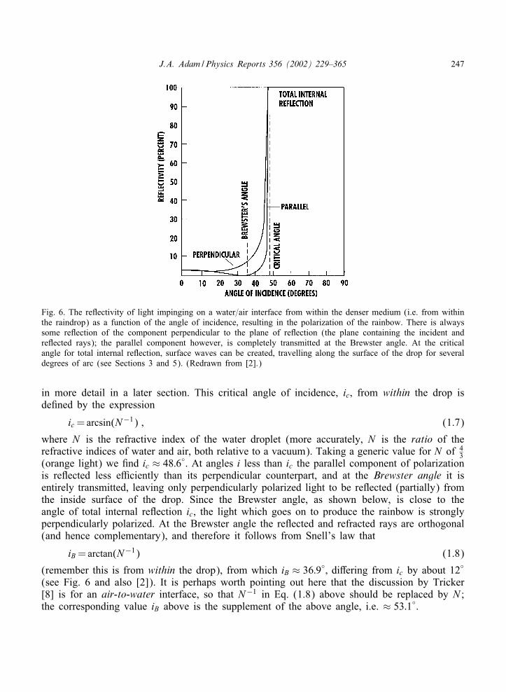
J.A. Adam /Physics Reports 356 (2002) 229–365 247
Fig. 6. The reTectivity of light impinging on a water=air interface from within the denser medium (i.e. from withinthe raindrop) as a function of the angle of incidence, resulting in the polarization of the rainbow. There is alwayssome reTection of the component perpendicular to the plane of reTection (the plane containing the incident andreTected rays); the parallel component however, is completely transmitted at the Brewster angle. At the criticalangle for total internal reTection, surface waves can be created, travelling along the surface of the drop for severaldegrees of arc (see Sections 3 and 5). (Redrawn from [2].)
in more detail in a later section. This critical angle of incidence, ic; from within the drop isdeAned by the expression
ic =arcsin(N−1) ; (1.7)
where N is the refractive index of the water droplet (more accurately, N is the ratio of therefractive indices of water and air, both relative to a vacuum). Taking a generic value for N of 4
3(orange light) we And ic ≈ 48:6◦: At angles i less than ic the parallel component of polarizationis reTected less eYciently than its perpendicular counterpart, and at the Brewster angle it isentirely transmitted, leaving only perpendicularly polarized light to be reTected (partially) fromthe inside surface of the drop. Since the Brewster angle, as shown below, is close to theangle of total internal reTection ic, the light which goes on to produce the rainbow is stronglyperpendicularly polarized. At the Brewster angle the reTected and refracted rays are orthogonal(and hence complementary), and therefore it follows from Snell’s law that
iB =arctan(N−1) (1.8)
(remember this is from within the drop), from which iB ≈ 36:9◦; di9ering from ic by about 12◦
(see Fig. 6 and also [2]). It is perhaps worth pointing out here that the discussion by Tricker[8] is for an air-to-water interface, so that N−1 in Eq. (1.8) above should be replaced by N ;the corresponding value iB above is the supplement of the above angle, i.e. ≈ 53:1◦:
248 J.A. Adam /Physics Reports 356 (2002) 229–365
The coeYcient of reTection of light depends on its degree of polarization: Consider Arstthe case of light polarized perpendicular to the plane of incidence, with the amplitude of theincident light taken as unity. It follows from the Fresnel equations that the fraction of theincident intensity reTected is [23]
sin2(r − i)sin2(r + i)
(1.9)
and
tan2(r − i)tan2(r + i)
; (1.10)
if the light is polarized parallel to the plane of incidence (there is an apparent discrepancybetween the terminology of Tricker [8] and Walker [14] at this point: in particular the diagramsin [8] for the Fresnel coeYcients as a function of i for an air-to-water interface have the oppositesense of polarization to that in [22,23] and other texts). It follows that for a ray entering a dropand undergoing k internal reTections (plus 2 refractions), the fraction of the original intensityremaining in the emergent ray is, for perpendicular polarization,
Ik1 =[1−(
sin2(r − i)sin2(r + i)
)]2(sin2(r − i)sin2(r + i)
)2k(1.11)
and for parallel polarization
Ik2 =[1−(
tan2(r − i)tan2(r + i)
)]2( tan2(r − i)tan2(r + i)
)2k: (1.12)
The total fraction is the sum of these two intensities. For angles of incidence close to normal,for which i ≈ Nr; it follows that the single-reTection intensity coeYcients for reTection andrefraction become, from Eq. (1.9)(
N − 1N + 1
)2(1.13)
and4N
(N + 1)2; (1.14)
respectively. For the choice of N = 43 under these circumstances it follows that the reTection
and refraction coeYcients are approximately 0:02 and 0:98, respectively.An alternative but entirely equivalent formulation of the Fresnel equations is applied to the
polarization of the (primary) rainbow in [35], using the relative amplitude equations for polar-ization both perpendicular to (E⊥) and parallel to the plane of incidence (E||) [36]. For eachpolarization, the emerging relative amplitude (i.e. scattered : incident) is determined by the prod-uct of the relative amplitudes corresponding to the three interfaces, namely transmission at anair=water interface, reTection at a water=air interface and transmission at a water=air interface(for rays 1, 2, 3 and 3′, respectively, in Fig. 1(c)). Care must be taken to identify the correctrefractive indices and angles of incidence, both of which depend on which medium the ray is
J.A. Adam /Physics Reports 356 (2002) 229–365 249
about to enter. The calculations (omitted in [35]) are straightforward but nonetheless worthy ofnote, and are summarized below. There are three interfaces to consider for the primary rainbowanalysis: air=water transmission (with transmission coeYcients t(1)s and t(1)p for the vector Eperpendicular and parallel to the plane of incidence, respectively); water=water re9ection (withcorresponding reTection coeYcients r(2)s ; r(2)p ), and water=air transmission (with transmissioncoeYcients t(3)s ; t(3)p ). Each will be considered in turn; in what follows n denotes the refractiveindex of the ‘incidence’ medium, n′ that of the ‘transmission’ medium, and as usual, i and rrepresent the angles of incidence and refraction. N is the refractive index of water; that of airwill be taken as unity. The formulae for the various coeYcients are taken from [36].
1.4.1. Air=water transmissionn=1; n′ =N = 4
3; at the (primary) rainbow angle (according to geometrical optics)
cos i=
√N 2 − 1
3from which the remaining quantities follow, so that
t(1)s =2 cos i
cos i +√
N 2 − sin2 i=
23
and
t(1)p =2N cos i
N 2 cos i +√
N 2 − sin2 i=
2N2 + N 2 :
1.4.2. Water=water re9ectionn=N = 4
3 ; n′ =1; in this case
sin r=1N
√4− N 2
3;
so that
r(2)s =N cos r −
√1− N 2 sin2 r
N cos r +√
1− N 2 sin2 r=
13
and
r(2)p =cos r − N
√1− N 2 sin2 r
cos r + N√
1− N 2 sin2 r=
2− N 2
2 + N 2 :
1.4.3. Water=air transmissionAgain, n=N = 4
3 ; n′ =1; and in this Anal situation
t(3)s =2N cos r
N cos i +√
1− N 2 sin2 r=
43
and
t(3)p =2N cos r
cos i + N√
1− N 2 sin2 r=
4N2 + N 2 :

250 J.A. Adam /Physics Reports 356 (2002) 229–365
These coeYcients are combined according to respective products
(i) t(1)s r(2)s t(3)s = 23
13
43 = 8
27
and
t(1)p r(2)p t(3)p =2N
2 + N 2
2− N 2
2 + N 2
4N2 + N 2 =2
(2− N 2
2 + N 2
)(2N
2 + N 2
)2so that the required relative amplitudes are
(1)Escatt
Einc= 8
27 (for E⊥) and (1:15)
Escatt
Einc= 2(
2NN 2 + 2
)2 (2− N 2
2 + N 2
)(for E||) :
It follows that the relative intensity of the perpendicular polarization (for N = 43) is 8:78% (i.e.
I⊥ ≈ 0:0878I0) and for the parallel polarization it is 0:34% (i.e. I|| ≈ 0:0034I0; note therefore,that I|| ≈ 0:039I⊥; so the primary bow is about 96% perpendicularly polarized).
Notice from Eq. (1.10) that the fraction of the intensity of reTected light is zero (for parallelpolarization) when the denominator in the coeYcient vanishes, i.e. when i+r=�=2; at this pointthe energy is entirely transmitted, so the internally reTected ray is completely perpendicularlypolarized. From this it follows that
sin i=N sin r=N cos i ;
whence
tan i= tan iB =N
for external reTection, and Eq. (1.8) for internal reTection. In the latter case, for N = 43, this
yields iB ≈ 36:9◦; the Brewster polarizing angle, as pointed out above. Note that as i+r “passesthrough” �=2; the tangent changes sign (obviously being undeAned at �=2); this correspondsto a phase change of 180◦ which will be noted when the so-called “glory” is discussed later.Notwithstanding the di9erences in terminology, it is also shown in [8], using Eqs. (1.11) and(1.12) that the primary rainbow is about 96% polarized (as shown above using Eqs. (1:15)),and the secondary bow somewhat less so: approximately 90%.
1.5. The physical basis for the divergence problem
In this subsection the physics of the di;erential scattering cross section is discussed (seethe deAnition of this in Appendix A). Referring to Fig. 7, note that for light incident upon theraindrop in the incidence interval (i; i + �i) the area “seen” by the incident rays is
(2�a sin i)(a cos i)�i
or
�a2�i sin 2i :

J.A. Adam /Physics Reports 356 (2002) 229–365 251
Fig. 7. The geometry leading to the derivation of the geometrical optics intensity function (1.15), which predictsinAnite intensity at the rainbow angle. (Redrawn from [8].)
These rays are then scattered into an interval (�; � + ��) say, measured from the direction ofincidence, and this results in solid angle of
(2� sin �)��
being occupied by these rays. Thus the energy (relative to incoming energy) entering unit solidangle per unit time after internal reTection (and neglecting losses from refraction and reTection)is
a2 sin 2i2 sin �
(�i��
): (1.15)
Passing to the limit, the Cartesian condition for the occurrence of the rainbow is of course thatd�=di=0, but now we are in possession of a geometric factor which modulates non-zero valuesof this derivative. This factor is undeAned when �=0 or � (these cases occurring when i=0),but for the case of a single internal reTection with both i and � “small”, using �=�−D=4r−2i,we have
limi→0+
sin 2isin �
=2i�
=2i
4r − 2i=
N2− N
: (1.16)
Since this ratio is just 2 when N = 43 it is clear that the intensity of the “backscattered” light
is not particularly large when �=0. This excludes, of course, any di9raction e9ects. Note thatfor large angles of incidence (i.e. i ≈ 90◦), the angle � (as deAned in Fig. 7) never returns tozero, being given instead by the expression
�=4 arcsin(N−1)− 180◦ ; (1.17)
which for N = 43 is approximately 14:4◦ according to geometrical optics (more will be said about
such grazing incidence rays when the glory is discussed in Section 3). Of course, it has alreadybeen noted that at the rainbow angle (corresponding to � ≈ 42◦) the intensity is predicted tobecome inAnite according to the same theory!
252 J.A. Adam /Physics Reports 356 (2002) 229–365
2. Theoretical foundations
2.1. The supernumerary rainbows; a heuristic account of Airy theory
These bows are essentially the result of interference between rays emerging from the raindropclose to the rainbow angle (i.e. angle of minimum deviation). In general they will have enteredat di9erent angles of incidence and traversed di9erent paths in the denser medium; there is ofcourse a reduction in wavelength inside the drop, but the overall e9ect of di9erent path lengthsis the usual “di9raction” pattern arising as a result of the destructive=constructive interferencebetween the rays. The spacing between the maxima (or minima) depends on the wavelengthof the light and the diameter of the drop—the smaller the drop the greater the spacing (seeFig. 4). Indeed, if the drops are less than about 0:2 mm in diameter, the Arst maximum willbe distinctly below the primary bow, and several other such maxima may be distinguished ifconditions are conducive.
Although this phenomenon is decidedly a “wavelike” one, we can gain some heuristic insightinto this mechanism by considering, following Tricker [8], a geometrical optics approach tothe relevant rays and their associated wavefronts. This is done by considering, not the angleof minimum deviation, but the point of emergence of a ray from the raindrop as the angle ofincidence is increased. A careful examination of Fig. 1(a) reveals that as the angle of incidenceis increased away from zero, while the point of entry moves clockwise around the drop, thepoint of emergence moves Arst in a counterclockwise direction, reaches an extreme position,and then moves back in a clockwise direction. This extreme point has signiAcant implicationsfor the shape of the wavefront as rays exit the drop in the neighborhood of this point. Referringto this Agure, we wish to And when angle BOA=4r − i is a maximum. This occurs when
drdi
=14
and
d2rdi2
¡ 0 :
The Arst derivative condition leads to
cos2 iN 2 − sin2 i
=16 (2.1)
or
i=arccos(N 2 − 1
15
)1=2; (2.2)
whence for N = 43, i ≈ 76:8◦, well past the angle of incidence corresponding to the rainbow
angle, which is i ≈ 59:4◦ for the same value of N . As can be seen from Fig. 8(a), if YEY ′represents the ray which emerges at minimum deviation, rays to either side of this are deviatedthrough larger angles as shown. By considering the corresponding wavefront WEW ′ (distortedfrom the wavefront XOX ′ (see Fig. 8(b)) corresponding to a parallel beam of rays) it is clear thatwe are dealing with, locally at least, a cubic approximation to the wavefront in the neighborhood
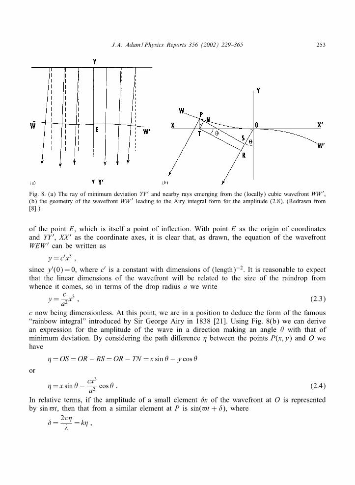
J.A. Adam /Physics Reports 356 (2002) 229–365 253
Fig. 8. (a) The ray of minimum deviation YY ′ and nearby rays emerging from the (locally) cubic wavefront WW ′,(b) the geometry of the wavefront WW ′ leading to the Airy integral form for the amplitude (2.8). (Redrawn from[8].)
of the point E, which is itself a point of inTection. With point E as the origin of coordinatesand YY ′, XX ′ as the coordinate axes, it is clear that, as drawn, the equation of the wavefrontWEW ′ can be written as
y= c′x3 ;
since y′(0)=0, where c′ is a constant with dimensions of (length)−2. It is reasonable to expectthat the linear dimensions of the wavefront will be related to the size of the raindrop fromwhence it comes, so in terms of the drop radius a we write
y=ca2 x
3 ; (2.3)
c now being dimensionless. At this point, we are in a position to deduce the form of the famous“rainbow integral” introduced by Sir George Airy in 1838 [21]. Using Fig. 8(b) we can derivean expression for the amplitude of the wave in a direction making an angle � with that ofminimum deviation. By considering the path di9erence % between the points P(x; y) and O wehave
%=OS =OR− RS =OR− TN = x sin �− y cos �
or
%= x sin �− cx3
a2 cos � : (2.4)
In relative terms, if the amplitude of a small element �x of the wavefront at O is representedby sin$t, then that from a similar element at P is sin($t + �), where
�=2�%�
= k% ;
254 J.A. Adam /Physics Reports 356 (2002) 229–365
� being the wavelength, and k being the wavenumber of the disturbance. For the whole wave-front the cumulative disturbance amplitude is therefore the integral
A=∫ ∞
−∞sin($t + k%) dx
or, since sin k% is an odd function,
A=sin$t∫ ∞
−∞cos k% dx : (2.5)
In terms of the following changes of variable:
+3 =2kcx3 cos �
�a2 (2.6)
and
m+=2kx sin �
�; (2.7)
the above integral may be written in the canonical form(�a2
2kc cos �
)1=3 ∫ ∞
−∞cos
�2(m+− +3) d+ : (2.8)
This is Airy’s rainbow integral, Arst published in his paper entitled “On the Intensity of Lightin the neighbourhood of a Caustic” [21]. The signiAcance of the parameter m can be noted byeliminating + from Eqs. (2.6) and (2.7) to obtain
m=(
2ka�
)2=3(sin3 �cos �
)1=3; (2.9)
which for suYciently small values of � (the angle of deviation from the rainbow ray) is pro-portional to �3.
A graph of the rainbow integral qualitatively resembles the di9raction pattern near the edgeof the shadow of a straight edge, which has the following features: (i) low-intensity, rapidlydecreasing illumination in regions that geometrical optics predicts should be totally in shadow,and (ii) in the illuminated region (as with di9raction), a series of fringes, which correspondto the supernumerary bows below the primary rainbow. The Arst maximum is the largest inamplitude, and corresponds to the primary bow; the remaining maxima decrease rather slowly inamplitude, the period of oscillation decreasing also. The underlying assumption in this approachis that di9raction arises from points on the wavefront in the neighborhood of the D7escartes ray(of minimum deviation); provided that the drop size is large compared to the wavelength oflight this is reasonable, and is in fact valid for most rainbows. It would not be as useful anassumption for cloud or fog droplets which are considerably smaller than raindrops, but eventhen the drop diameter may be Ave or ten times the wavelength, so the Airy theory is stilluseful. Clearly, however, it has a limited domain of validity.
J.A. Adam /Physics Reports 356 (2002) 229–365 255
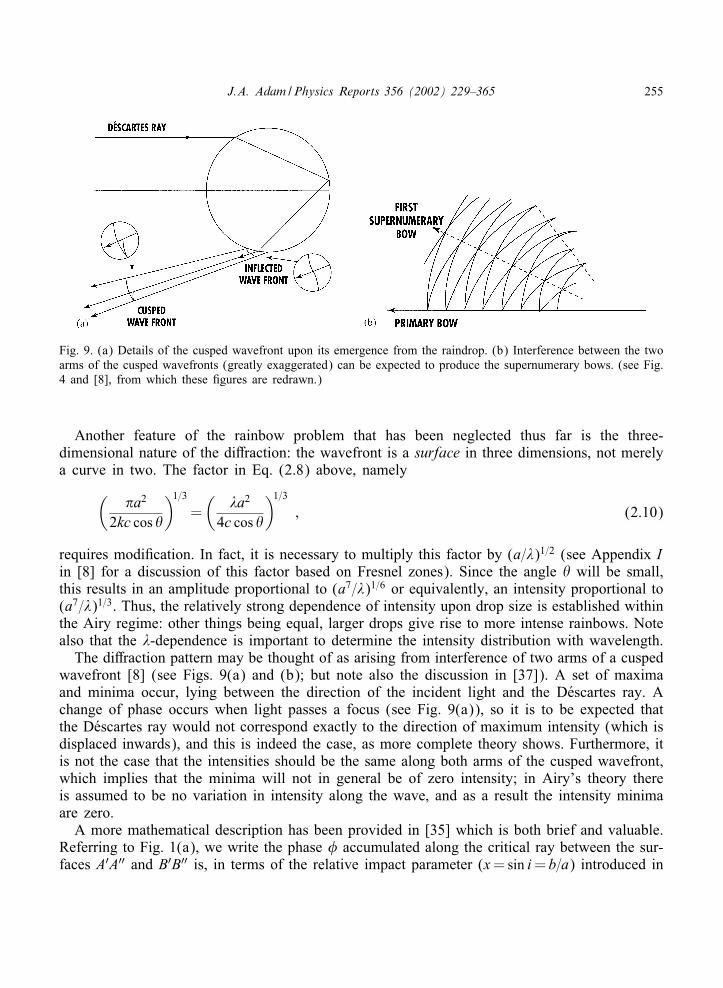
Fig. 9. (a) Details of the cusped wavefront upon its emergence from the raindrop. (b) Interference between the twoarms of the cusped wavefronts (greatly exaggerated) can be expected to produce the supernumerary bows. (see Fig.4 and [8], from which these Agures are redrawn.)
Another feature of the rainbow problem that has been neglected thus far is the three-dimensional nature of the di9raction: the wavefront is a surface in three dimensions, not merelya curve in two. The factor in Eq. (2.8) above, namely
(�a2
2kc cos �
)1=3=(
�a2
4c cos �
)1=3; (2.10)
requires modiAcation. In fact, it is necessary to multiply this factor by (a=�)1=2 (see Appendix Iin [8] for a discussion of this factor based on Fresnel zones). Since the angle � will be small,this results in an amplitude proportional to (a7=�)1=6 or equivalently, an intensity proportional to(a7=�)1=3. Thus, the relatively strong dependence of intensity upon drop size is established withinthe Airy regime: other things being equal, larger drops give rise to more intense rainbows. Notealso that the �-dependence is important to determine the intensity distribution with wavelength.
The di9raction pattern may be thought of as arising from interference of two arms of a cuspedwavefront [8] (see Figs. 9(a) and (b); but note also the discussion in [37]). A set of maximaand minima occur, lying between the direction of the incident light and the D7escartes ray. Achange of phase occurs when light passes a focus (see Fig. 9(a)), so it is to be expected thatthe D7escartes ray would not correspond exactly to the direction of maximum intensity (which isdisplaced inwards), and this is indeed the case, as more complete theory shows. Furthermore, itis not the case that the intensities should be the same along both arms of the cusped wavefront,which implies that the minima will not in general be of zero intensity; in Airy’s theory thereis assumed to be no variation in intensity along the wave, and as a result the intensity minimaare zero.
A more mathematical description has been provided in [35] which is both brief and valuable.Referring to Fig. 1(a), we write the phase , accumulated along the critical ray between the sur-faces A′A′′ and B′B′′ is, in terms of the relative impact parameter (x=sin i= b=a) introduced in
256 J.A. Adam /Physics Reports 356 (2002) 229–365
Section 1.3,
,(x)= ka{2(1− cos i) + 4N cos r}=2ka{1−
√1− x2 + 2
√N 2 − x2} :
The Arst term inside the Arst set of brackets is the sum of the distances from both A′′ and B′′ tothe surface of the drop; the second term is N times the path length interior to the drop. Notingthat
,′x(x)=2ka{
x√1− x2
− 2x√N 2 − x2
}
and comparing this with the result derived in Section 1 for the derivative with respect to x ofthe deTection angle �(x) it is seen that
,′(x)= kax�′(x) :
Near the critical angle �= �0 (and hence near x= x0) this result may be written in terms of thevariable += x − x0, i.e.
,′(+)= ka[x0�′(+) + +�′(+)] ;
whence
,(+)=,0 + ka
[x0(�− �0) + +�(+)−
∫ +′
0�(+′) d+′
]:
Using the result, previously derived, that near �= �0,
�(+) ≈ �0 + �′′(�0)+2=2 + O(+3) ;
it is readily shown that
,(+) ≈ ,0 + ka[x0(�− �0) + �′′(�0)+3=3 + O(+4) ;
so that for two rays, each one close to, but on opposite sides of the critical ray, with equal andopposite +-values, it follows that their phase di9erence � is
�=,(+)− ,(−+) ≈ 2ka�′′(�0)+3=3 :
When a phase di9erence is equal to an integer multiple of 2� then the rays interfere construc-tively in general; however, in this instance (and as noted above) an additional �=2 must beadded because a focal line is passed in the process (see [7, chapters 12 and 13]). Hence forconstructive interference
�K − �0 ≈(
3�(K + 14)
ka
)2=3 [�′′(�0)
8
]1=3; K =1; 2; : : : :
Clearly, within this approximation, �K − �0 ˙ (ka)−2=3 which is quite sensitive to droplet size.If the droplets are large enough, the supernumerary bows lie inside the primary bow and thus
J.A. Adam /Physics Reports 356 (2002) 229–365 257
are not visible; Jackson demonstrates that the maximum uniform droplet size rendering themvisible is a � 0:28 mm [35]. If the droplets are not uniform in size, the maxima may be washedout by virtue of the spread in sizes; if the droplets are all very small (a¡ 50 �m) the variouscolors are dispersed little and “whitebows” or “cloudbows” result.
To capitalize on the expressions for the phase function ,(x) and �− �0, refer now in Agure(∗) to the wavefront along BB′; following [35], it can be shown using the Kircho9 integral fordi9raction that the amplitude of the scattered wave near �= �0 is
scatt ˙∫ ∞
−∞eika[(�−�0)+−�′′+3=6] d+ :
This can be expressed in the form of an Airy integral Ai(−%) (essentially equivalent to Eq.(2.8), which is the form given in [7]), where
Ai(−%)=1�
∫ ∞
0cos(
13+3 − %+
)d+ ;
where
%=(
2k2a2
�′′(�0)
)1=3(�− �0) :
For more details of the Airy function and the relationship between the two forms, see AppendixB. For large values of %¿ 0 the dominant term in the asymptotic expansion for Ai(−%) is
Ai(−%) � (�2%)−1=4 sin(
23%3=2 +
�4
)
corresponding to slowly decaying oscillations on the “bright” side of the primary bow (for%¡ 0, Ai(−%) decreases to zero faster than exponentially; this is the “shadow” side of theprimary bow). Noting that [35]
〈|Ai(−%)|2〉=(2�√%)−1 ;
where 〈:〉 means the average value of its argument, it may be veriAed that
〈|Ai(−%)|2〉= 12�
(�′′2(�0)4ka
)1=3√ 2�′′(�0)(�− �0)
:
Near �= �0, the classical di9erential scattering cross section has been found to be
d/d0 class
≈(
a2x0sin �0
)√2
|�′′(�0)(�− �0)|(the factor a2 appearing because x is dimensionless). By comparing this directly with the meansquare Airy intensity, an approximate expression for the “Airy di9erential cross section” can beinferred, namely
d/d0Airy
≈(
2�a2x0sin �0
)(4ka
�′′2(�0)
)1=3|Ai(−%)|2 :

258 J.A. Adam /Physics Reports 356 (2002) 229–365
If the intensity loss from two refractions and one reTection are ignored (they cannot be)this cross section is about 30 times as great as that for an isotropic di9erential cross sec-tion (d/=d0= a2=4) at the peak of the primary bow when ka=103. This must be multiplied bythe scattered=incident ratios calculated in Section 1.4 when these intensity losses are included.This renders the two cross sections comparable in magnitude [35].
The extension of the Airy theory to incorporate the superposition of light of all colors wasArst carried out by Pernter and Exner [38] in 1910, and later by Buchwald [39], who cor-rected some errors in the former work. The methods and results for the Airy–Pernter theoryare well summarized by Tricker, and only a few speciAc results will be noted here. From thebasic di9raction theory discussed so far, it is reasonable to expect supernumerary bows to existoutside the secondary bow (in the region of low-intensity illumination). Because of the widthof the secondary—more than twice that of the primary—the displacements of the individualcolor interference patterns will be larger, and whiter, weaker supernumerary bows are to beexpected, which, coupled with the lower intensity of the secondary bow means that such su-pernumeraries are rarely observed. Another point to be mentioned here involves polarization:changes in polarization can be neglected only if the plane of incidence of sunlight on the dropvaries by a small angle, which in turn means that integral (2.8) should extend (in practice)only over those portions of the wavefront in the neighborhood of the D7escartes ray. This isclearly another limitation of the theory as originally formulated. Malkus et al. attempted toimprove upon the Airy–Pernter theory by developing a better approximation to the shape of thewavefront (amongst other things), subsequently applying their theory to cloud (as opposed torain) droplets, with mixed success [40].
2.2. Mie scattering theory
Mie theory is based on the solution of Maxwell’s equations of electromagnetic theory fora monochromatic plane wave from inAnity incident upon a homogeneous isotropic sphere ofradius a. The surrounding medium is transparent (as the sphere may be), homogeneous andisotropic. The incident wave induces forced oscillations of both free and bound charges in syn-chrony with the applied Aeld, and this induces a secondary electric and magnetic Aeld, each ofwhich has a components inside and outside the sphere [41] (see also [9,10]).
In what follows reference will be made to the intensity functions i1; i2, the Mie coeYcientsan; bn and the angular functions �n; 1n. The former pair are proportional to the (magnitude)2 oftwo incoherent, plane-polarized components scattered by a single particle; they are related tothe scattering amplitudes S1 and S2 in the notation of Nussenzveig [10]. The function i1(; N; �)is associated with the electric oscillations perpendicular to the plane of scattering (sometimescalled horizontally polarized) and i2(; N; �) is associated with the electric oscillations parallelto the plane of scattering (or vertically polarized). The scattered wave is composed of manypartial waves, the amplitudes of which depend on an(; N ) and bn(; N ). Physically, thesemay be interpreted as the nth electrical and magnetic partial waves, respectively. The intensityfunctions i1; i2 are represented in Mie theory as a spherical wave composed of two sets ofpartial waves: electric (an) and magnetic (bn). The Arst set is that part of the solution forwhich the radial component of the magnetic vector in the incident wave is zero; in the second
J.A. Adam /Physics Reports 356 (2002) 229–365 259
set the corresponding radial component of the electric vector is zero. A given partial wave canbe thought of as coming from an electric or a magnetic multipole Aeld, the Arst wave comingfrom a dipole Aeld, the second from a quadrupole, and so on [41]. The angular functions �n(�)and 1n(�) are, as their name implies, independent of size () and refractive index (N ). Theseare investigated in some detail by Penndorf [41] in connection with scattering in the forward,backward and side directions for N =1:33.
For a point P located a distance r from the origin of coordinates, at polar angle � andazimuthal angle , the scattered intensities I� and I, are, respectively,
I� =(
i2kr
)2cos2 , (2.11)
and
I, =(
i1kr
)2sin2 , ; (2.12)
where ij = |Sj|2; j=1; 2 and the amplitude functions Sj are given by
S1 =∞∑n=1
2n + 1n(n + 1)
[an�n(cos �) + bn1n(cos �)] (2.13)
and
S2 =∞∑n=1
2n + 1n(n + 1)
[an1n(cos �) + bn�n(cos �)] ; (2.14)
where n is the order of the induced electric or magnetic multipole. The Legendre functions�n(cos �) and 1n(cos �) are deAned in terms of the associated Legendre functions of the Arstkind, P1
n(cos �) as
�n(cos �)=P1
n(cos �)sin �
(2.15)
and
1n(cos �)=dd�
P1n(cos �) : (2.16)
The scattering coeYcients an and bn are deAned in terms of the so-called Ricatti–Besselfunctions of the Arst and second kinds, respectively, these being
n(z)=√
�z2Jn+1=2(z) and 4n(z)= (−1)n
√�z2J−(n+1=2)(z) :
Also note that a Riccati–Hankel function is readily deAned by
+n(z)= n(z) + i4n(z) :
260 J.A. Adam /Physics Reports 356 (2002) 229–365
Then it follows that an and bn can be written
an = n() ′
n(5)− N n(5) ′n()
+n() ′n(5)− N n(5)+′n()
(2.17)
and
bn = n(5) ′
n()− N n() ′n(5)
+′n() n(5)− N ′n(5)+n()
; (2.18)
where the usual dimensionless size parameters are = ka and 5=N. This form can be sim-pliAed by the introduction of phase angles; and this results in considerable simpliAcation if therefractive index is real. Further details of the analysis may be found in the book by van deHulst [7]; for an alternative but entirely equivalent formulation see [10]. Van de Hulst demon-strated that the Mie formulae lead, for large values of ; to a principle for localizing rays andseparating di9racted, refracted and reTected light (in the sense of geometrical optics). This iscalled the localization principle and will be utilized in connection with the theories of the gloryin Section 3 and the CAM approach to rainbows and glories in Section 5. The principle assertsthat the term of order n in the partial wave expansion corresponds approximately to a ray ofdistance (n + 1
2)=k from the center of the particle (this is just the impact parameter). When�1, the expansions for the Sj may be truncated at n+ 1
2 � (in practice, nmax ∼ +41=3+2;see [5,10,42]) and the remaining sum is separated into two parts: a di9racted light Aeld com-ponent independent of the nature of the particle, and reTected and refracted rays dependent onthe particle (see also [43–46]). In the former case both amplitude functions are equal to thequantity
2 J1( sin �)( sin �)
; (2.19)
a result we shall have occasion to refer to later.
3. Glories
3.1. The backward glory
Mountaineers and hill-climbers have noticed on occasion that when they stand with theirbacks to the low-lying sun and look into a thick mist below them, they may sometimes see aset of colored circular rings (or arcs thereof) surrounding the shadow of their heads. Althoughan individual may see the shadow of a companion, the observer will see the rings only aroundhis or her head. This is the phenomenon of the glory, sometimes known at the anticorona, thebrocken bow, or even the specter of the Brocken (it being frequently observed on this high peakin the Harz mountains of central Germany). A brief but very useful historical account (based on[38]), along with a summary of the theories, can be found in [47]. Early one morning in 1735,a small group of people were gathered on top of a mountain in the Peruvian Andes, membersof a French scientiAc expedition, sent out to measure a degree of longitude, led by Bouguer
J.A. Adam /Physics Reports 356 (2002) 229–365 261
and La Condamine; a Spanish captain named Antonio de Ulloa also accompanied them. Theysaw an amazing sight that morning. According to Bouguer [38] this was
“a phenomenon which must be as old as the world, but which no one seems to haveobserved so far: : : A cloud that covered us dissolved itself and let through the rays of therising sun: : : Then each of us saw his shadow projected upon the cloud: : : The closenessof the shadow allowed all its parts to be distinguished: arms, legs, the head. What seemedmost remarkable to us was the appearance of a halo or glory around the head, consistingof three or four small concentric circles, very brightly colored, each of them with the samecolors as the primary rainbow, with red outermost.”
Ulloa gave a similar description and also drew a picture. In his account he said
“The most surprising thing was that, of the six or seven people that were present, each onesaw the phenomenon only around the shadow of his own head, and saw nothing aroundother people’s heads.”
During the 19th century, many such observations of the glory were made from the top of theBrocken mountain in central Germany, and it became known as the “Specter of the Brocken”.It also became a favorite image among the Romantic writers; it was celebrated by Coleridge inhis poem “Constancy to an Ideal Object”. Other sightings were made from balloons, the gloryappearing around the balloon’s shadow on the clouds. Nowadays, while not noted as frequentlyas the rainbow, it may be seen most commonly from the air, with the glory surrounding theshadow of the airplane. Once an observer has seen the glory, if looked for, it is readily found onmany subsequent Tights (provided one is on the shadow side of the aircraft!). Some beautifulcolor photographs have appeared in the scientiAc literature [4,48,49].
The phenomenon in simplest terms is essentially the result of light backscattered by clouddroplets, the light undergoing some unusual transformations en route to the observer, transfor-mations not predictable by standard geometrical optics (see the summary of contributing factorslisted below). In a classic paper ([50]; later incorporated into his book [7]) van de Hulst putforward his theory of the glory, though at that time the term anti-corona was commonly usedfor this phenomenon. Noting that glories typically occur for cloud drop diameters of the or-der of 25 �m ( ≈ 150), he used the asymptotic forms for the Legendre functions (sphericalharmonics) �n and 1n above, namely
�n(cos �)= (−1)n−1 12n(n + 1){J0(z) + J2(z)} (3.1)
and
1n(cos �)= (−1)n 12n(n + 1){J0(z)− J2(z)} ; (3.2)
where as before, n is the order of the induced electric or magnetic multipole, z=(n+ 12)6 and
6=�−� is small (note that in [42] z is deAned as n6). Under these circumstances the amplitudefunctions S1(�) and S2(�) in the backward direction have the form
S1(180◦)=− S2(180
◦)=∞∑n=1
12(2n + 1)(−1)n(bn − an) : (3.3)
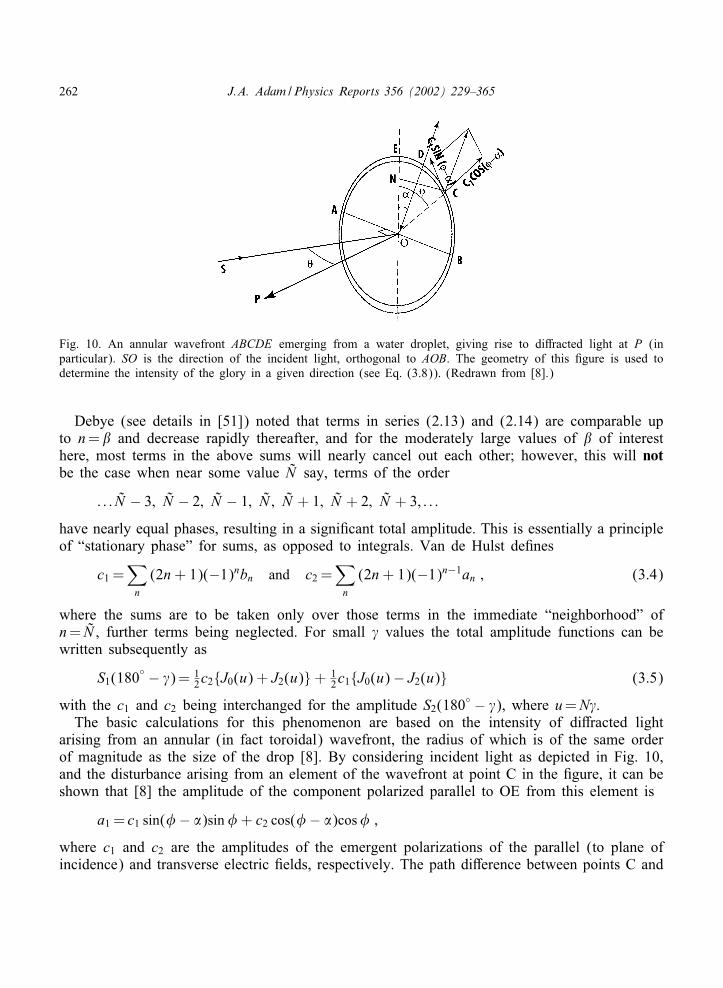
262 J.A. Adam /Physics Reports 356 (2002) 229–365
Fig. 10. An annular wavefront ABCDE emerging from a water droplet, giving rise to di9racted light at P (inparticular). SO is the direction of the incident light, orthogonal to AOB. The geometry of this Agure is used todetermine the intensity of the glory in a given direction (see Eq. (3.8)). (Redrawn from [8].)
Debye (see details in [51]) noted that terms in series (2.13) and (2.14) are comparable upto n= and decrease rapidly thereafter, and for the moderately large values of of interesthere, most terms in the above sums will nearly cancel out each other; however, this will notbe the case when near some value N say, terms of the order
: : : N − 3; N − 2; N − 1; N ; N + 1; N + 2; N + 3; : : :
have nearly equal phases, resulting in a signiAcant total amplitude. This is essentially a principleof “stationary phase” for sums, as opposed to integrals. Van de Hulst deAnes
c1 =∑n
(2n + 1)(−1)nbn and c2 =∑n
(2n + 1)(−1)n−1an ; (3.4)
where the sums are to be taken only over those terms in the immediate “neighborhood” ofn= N , further terms being neglected. For small 6 values the total amplitude functions can bewritten subsequently as
S1(180◦ − 6)= 1
2c2{J0(u) + J2(u)}+ 12c1{J0(u)− J2(u)} (3.5)
with the c1 and c2 being interchanged for the amplitude S2(180◦ − 6), where u=N6.
The basic calculations for this phenomenon are based on the intensity of di9racted lightarising from an annular (in fact toroidal) wavefront, the radius of which is of the same orderof magnitude as the size of the drop [8]. By considering incident light as depicted in Fig. 10,and the disturbance arising from an element of the wavefront at point C in the Agure, it can beshown that [8] the amplitude of the component polarized parallel to OE from this element is
a1 = c1 sin(,− 5)sin, + c2 cos(,− 5)cos, ;
where c1 and c2 are the amplitudes of the emergent polarizations of the parallel (to plane ofincidence) and transverse electric Aelds, respectively. The path di9erence between points C and
J.A. Adam /Physics Reports 356 (2002) 229–365 263
E in the direction OP is �= r sin, sin �, and the phase di9erence is 2��=� ≡ x sin,. The totalamplitude polarized parallel to OE from the whole wavefront is, after some reduction (and usingantisymmetry of the cosine between the Arst and second quadrants)
A1 = c1 cos 5∫ 2�
0
1− cos 2,2
cos(x sin,) d, + c2 cos 5∫ 2�
0
1 + cos 2,2
cos(x sin,) d, ;
which to within a multiplicative factor is
A1 = cos 5(c1{J0(x)− J2(x)}+ c2{J0(x) + J2(x)}) : (3.6)
Similarly, for the perpendicular polarization
A2 = sin 5(c1{J0(x) + J2(x)}+ c2{J0(x)− J2(x)}) : (3.7)
For unpolarized light the direction of polarization changes rapidly and randomly, so little islost by replacing the terms cos2 5 and sin2 5 in the intensity by their averages (1
2) to obtain
I =A21 + A2
2 = (c1 + c2)2J 20 (x) + (c1 − c2)2J 2
2 (x) : (3.8)
The observational consequences of various choices of c1 and c2 (e.g. c1 =± c2; c1 =0) can befound in Section 13:33 of [7]. Tricker [8] makes the choice c2 =− 0:204c1 based on a rainbowwith 96% polarization in the plane of incidence (c2
2=c21 =4=96), and incorporating the change in
phase as the Brewster angle is exceeded (see also [50]). Fig. 10 is based on his calculations.Further descriptive (and also historical) details may be found in [52].
More can be said about the glory from a purely geometrical optics viewpoint. Recall that,for the heuristic description of the rainbow (Section 1.5) an important geometrical factor in theamplitude was shown to be∣∣∣∣sin 2i
sin �did�
∣∣∣∣1=2
:
As noted already, rainbows correspond (at this level of description) to the condition d�=di=0,i.e. inAnite intensity is predicted at the rainbow angle when interference is neglected. Such adivergence also occurs when sin �=0 while sin 2i �=0; which occurs for �=0 and �. The fea-tures associated with the forward direction are blended with the stronger coronae caused by thedi9raction of light around the spherical drop [7], but the backward direction corresponds to theglory. Notice from Fig. 11 that the plane wavefront of the incident wave is emitted as a circularfront, which has a virtual focus at F; when the Agure is rotated about the axis of symmetry,the emitted wavefront is seen to be toroidal. Furthermore, this wavefront apparently emergesfrom the focal circle deAned by Huygens’ principle can be used to describe the interferencepattern corresponding to this wavefront. Note that for a refractive index N ¡
√2 there can be
no such o9-axis rays with less than four internal reTections contributing to the glory [7], butthe attenuation for these rays is such that their contribution is negligible [53]. Thus accordingto ray theory, only the axial rays can contribute to this phenomenon.
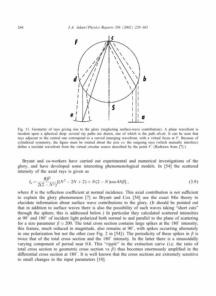
264 J.A. Adam /Physics Reports 356 (2002) 229–365
Fig. 11. Geometry of rays giving rise to the glory (neglecting surface-wave contribution). A plane wavefront isincident upon a spherical drop: several ray paths are drawn, one of which is the path abcde. It can be seen thatrays adjacent to the central one correspond to a curved emerging wavefront, with a virtual focus at F . Because ofcylindrical symmetry, the Agure must be rotated about the axis cs; the outgoing rays (which mutually interfere)deAne a toroidal wavefront from the virtual circular source described by the point F . (Redrawn from [7].)
Bryant and co-workers have carried out experimental and numerical investigations of theglory, and have developed some interesting phenomenological models. In [54] the scatteredintensity of the axial rays is given as
Ia =R2
2(2− N 2)[(N 2 − 2N + 2) + N (2− N )cos 4N] ; (3.9)
where R is the reTection coeYcient at normal incidence. This axial contribution is not suYcientto explain the glory phenomenon [7] so Bryant and Cox [54] use the exact Mie theory toelucidate information about surface wave contributions to the glory. (It should be pointed outthat in addition to surface waves there is also the possibility of such waves taking “short cuts”through the sphere; this is addressed below.) In particular they calculated scattered intensitiesat 90◦ and 180◦ of incident light polarized both normal to and parallel to the plane of scatteringfor a size parameter � 200. The total cross section contains large spikes at the 180◦ intensity;this feature, much reduced in magnitude, also remains at 90◦; with spikes occurring alternatelyin one polarization but not the other (see Fig. 2 in [54]). The periodicity of these spikes in istwice that of the total cross section and the 180◦ intensity. In the latter there is a sinusoidallyvarying component of period near 0:8. This “ripple” in the extinction curve (i.e. the ratio oftotal cross section to geometric cross section vs ) thus becomes enormously ampliAed in thedi9erential cross section at 180◦. It is well known that the cross sections are extremely sensitiveto small changes in the input parameters [10].
J.A. Adam /Physics Reports 356 (2002) 229–365 265
Mention has been made already of the localization principle: terms of order n in the Mieexpansion correspond to a ray passing the origin at a distance (n+ 1
2)=k because as is known inconnection with partial-wave analysis, the nth partial wave is associated with angular momentum
M =√
n(n + 1)˜ ∼ bn =(n + 12)˜
(the last approximation being valid for large values of n). The appropriate impact parametersare concentrated within the annular region [n�=2�; (n + 1
2)�=2�]; and for the mid-range impactparameter bn; M =pbn, where p is the incident linear momentum, which in the semiclassicalapproximation is associated classically with a particle of momentum h=�. Hence
bn ≈(n + 1
2)k
:
The convergence of the Mie expansion for n&= ka is (physically) a consequence of the factthat the rays no longer interact with the scattering sphere (again, though, this is not the completepicture; as has been noted in the introduction, tunneling to the surface can occur for impactparameters greater than a, giving rise to the sharp resonances found in the ripple: this willbe further elaborated in Section 5). The results for the scattering at 180◦ indicate that theyare determined almost entirely by rays nearly tangential to the surface together with a smallercontribution from the axial rays.
Based on these results, an interesting phenomenological model for the surface waves wasdeveloped in [54]. The idea is that a tangentially incident bundle of rays is trapped on thespherical surface and propagates around it with constant attenuation due to reradiation. In termsof unit amplitude at its point of tangential entry at 0◦, at 90◦ it is A; A2 at 180◦; A3 at 270◦,and so on, where |A|¡ 1: The scattering amplitude at 0◦ can be represented as
S(0◦)= 5(1 + A4 + A8 + A12 + · · ·) + B ; (3.10)
where 5 is a real constant, and the term B represents the contribution to zero-degree scatteringfrom other mechanisms. Clearly
S(0◦)= 5(1− A4)−1 + B ; (3.11)
so writing A4 = bei, and using the optical theorem [7] in the form
Q=4Re[S(0◦)]−2 ; (3.12)
Q being the extinction coeYcient, it is found that
Q=Q0 +452
(1− b cos,
1 + b2 − 2b cos,
); (3.13)
where Q0 is determined by the term B. The authors then consider a region of resonance near,=2m�; m being an integer and , being replaced by ,mod 2�: Thus it follows that if b=e−g
and , and g are both small
Q(,) ≈ D1
1 + (,=g)2+ D2 ; (3.14)
266 J.A. Adam /Physics Reports 356 (2002) 229–365
where D1 and D2 are insensitive to small changes in ,: The period of this peak is 0:809,so ,=2�=0:809, and the authors At the equation for Q(,) to their numerical results for Q,yielding a value for g=0:008. This means that b ≈ 0:99, and this represents the attenuationaround one circumference of the drop. Being so small, it implies that the peak is an interferencemaximum involving tens, perhaps even hundreds of circuits by the surface wave. A similarargument for �=180◦ yields
S(180◦)= 5A2(1− A4)−1 + B′ (3.15)
with a corresponding expression for the intensity |S(180◦)|2; if the 90◦ and 270◦ scatteringamplitudes are combined then
S(90◦=270◦)= 5A(1− A2)−1 + B′′ (3.16)
and from the deAnition of , it is clear that the resonances at 90◦ have twice the period that isexhibited by S(180◦) and Q.
In a subsequent comparison of experimental results with Mie theory, Fahlen and Bryant[55] developed a two-parameter scalar model in an attempt to gain insight into the scatteringmechanisms involved in the scattering data they acquired. Their model again involved surfacewaves; such waves transport energy tangential to the interface between two media, and ariseswhen that energy strikes such an interface (between two dielectric media) from the more denseside at or exceeding the critical angle for total reTection (allowing for a limiting process for theinitial interaction from the less dense side). It is known from several experiments [56,57] thatas a surface wave travels along the interface, it continuously reradiates energy back into thedenser medium at the angle of critical refraction. It is also attenuated by “spraying” o9 energytangentially as it propagates around the drop surface. Part of the energy refracted back into thedrop (the short cut component) is reTected internally and the remaining part interferes with thesurface wave; this occurs over the course of many revolutions around the drop. For a drop ofradius a it is shown that the total optical path length for a ray performing M revolutions aroundthe drop and n jumps (short cuts) across it is
l(n;M)=2�Ma + �a + 2na(tan 5− 5) ; (3.17)
where � is the scattering angle subtended by both the chord and the arc AB (see Fig. 12).Denoting the amplitude of such a ray by A(n;M), the probability (statistical weight in [55]) forn jumps by P(n;M) and the surface wave attenuation by exp(−6z), z being the surface distancedeAned by
z=2�Ma + �a− 2n5a ;
then
A(n;M)=P(n;M) exp[− 6z + 2�il(n;M)=�] : (3.18)
The (complex) total amplitude At is the sum of all possible paths, i.e.
At =∞∑
M=0
n∗∑n=0
A(n;M) ; (3.19)
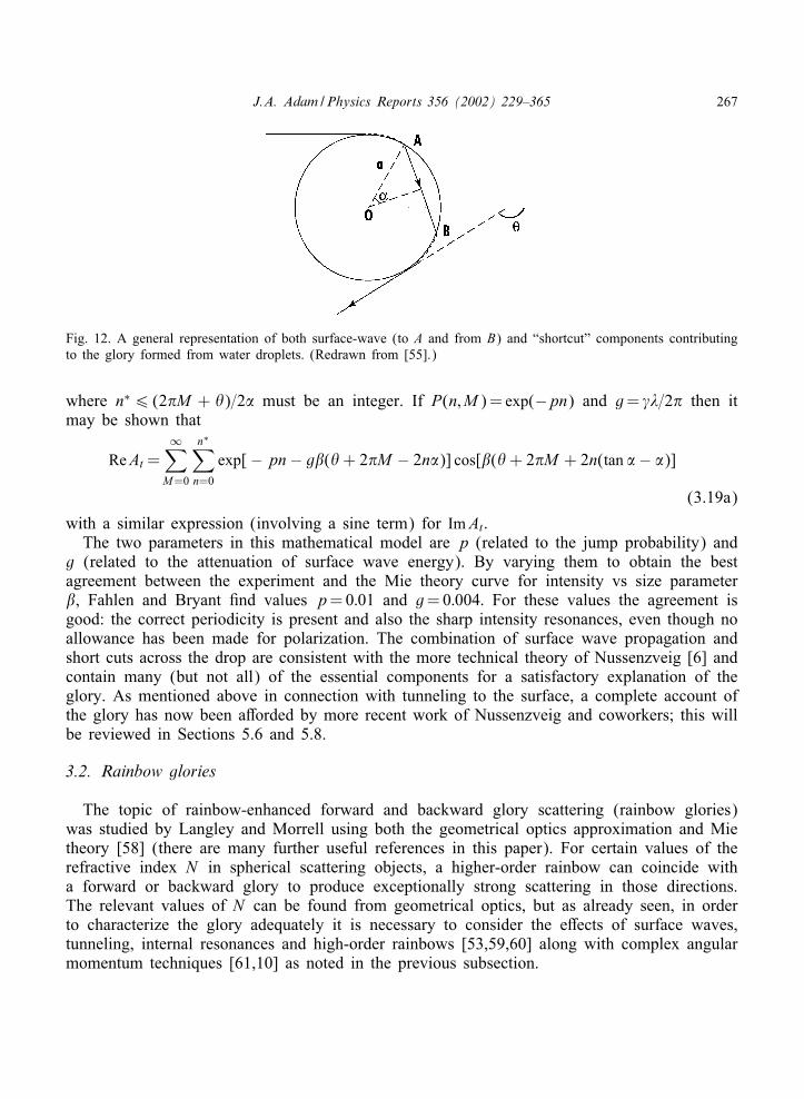
J.A. Adam /Physics Reports 356 (2002) 229–365 267
Fig. 12. A general representation of both surface-wave (to A and from B) and “shortcut” components contributingto the glory formed from water droplets. (Redrawn from [55].)
where n∗6 (2�M + �)=25 must be an integer. If P(n;M)= exp(−pn) and g= 6�=2� then itmay be shown that
ReAt =∞∑
M=0
n∗∑n=0
exp[− pn− g(� + 2�M − 2n5)] cos[(� + 2�M + 2n(tan 5− 5)]
(3.19a)
with a similar expression (involving a sine term) for ImAt:The two parameters in this mathematical model are p (related to the jump probability) and
g (related to the attenuation of surface wave energy). By varying them to obtain the bestagreement between the experiment and the Mie theory curve for intensity vs size parameter, Fahlen and Bryant And values p=0:01 and g=0:004: For these values the agreement isgood: the correct periodicity is present and also the sharp intensity resonances, even though noallowance has been made for polarization. The combination of surface wave propagation andshort cuts across the drop are consistent with the more technical theory of Nussenzveig [6] andcontain many (but not all) of the essential components for a satisfactory explanation of theglory. As mentioned above in connection with tunneling to the surface, a complete account ofthe glory has now been a9orded by more recent work of Nussenzveig and coworkers; this willbe reviewed in Sections 5.6 and 5.8.
3.2. Rainbow glories
The topic of rainbow-enhanced forward and backward glory scattering (rainbow glories)was studied by Langley and Morrell using both the geometrical optics approximation and Mietheory [58] (there are many further useful references in this paper). For certain values of therefractive index N in spherical scattering objects, a higher-order rainbow can coincide witha forward or backward glory to produce exceptionally strong scattering in those directions.The relevant values of N can be found from geometrical optics, but as already seen, in orderto characterize the glory adequately it is necessary to consider the e9ects of surface waves,tunneling, internal resonances and high-order rainbows [53,59,60] along with complex angularmomentum techniques [61,10] as noted in the previous subsection.
268 J.A. Adam /Physics Reports 356 (2002) 229–365
The total deviation angle D undergone by a ray is, in the present notation,
D=2i − 2rP + (P − 1)� : (3.20)
Forward and backward scattering correspond to D=L�; so from this relation and Snell’s lawthe glory condition is found to be
N =(csc r) cos{rP − �(P − L)=2} : (3.21)
The ray paths may be conveniently designated by the ordered pair (P; L) where P is thenumber of chords the ray makes inside the sphere and L is the number of times the ray crossesthe optical axis. The authors demonstrate that for a given N there may be 0; 1 or 2 glory raysof type (P; L) with the following ranges:
3.2.1. Ray
sec(L�=2P)¿N ¿ 0; P − 1¿L ;
csc(�=2P)6N6P; P − 1=L :
3.2.2. Rays
sec(L�=2P)6N6N ∗; P − 1¿L¿ 0 :
N ∗ is the refractive index for which a rainbow coincides with a glory; using the (necessary)rainbow condition dD=di=0 is, on using Snell’s law and Eq. (3.20),
tan i=P tan r : (3.22)
The requirement that both the rainbow and glory conditions be satisAed is therefore
P tan r=B(tan rP)B (3.23)
where B=(−1)P−L−1: For a given (P; L) the solution of this equation for r when substitutedin (3.21) gives the value of N ∗. A table of eight such values can be found in [58] along withdetailed Agures and calculations for the physical optics approximation and the Mie theory; wenote several features here. By comparing incremental areas of the wavefront entering and exitingthe sphere, the parameter A=2(P tan r − tan i) occurs, where A is zero at the rainbow angle.Using this parameter, the radius of curvature of the wavefront at the exit plane is deAned to be
Q(N )=A
A + sin i:
Q=0 corresponds to a cubic wavefront, but the glory wavefront may be diverging (Q¿ 0) orconverging (Q¡ 0) at the exit plane, depending on the value of N: Many of the mathematicaldetails follow from the earlier work [62,63]. Normal glory scattering leads to an irradiance withsize parameter dependence O(); for a rainbow-enhanced glory this becomes O(4=3), based onthe physical optics approximation, and the Mie theory calculations conArm this at the predictedvalues of N: The polarization properties of rainbow glories are found to be similar to those fornormal glory scattering.
J.A. Adam /Physics Reports 356 (2002) 229–365 269
3.3. The forward glory
The optical glory is a strong enhancement in near-backward scattering of light from waterdroplets with size parameter &100, arising from a combination of almost grazing incident rays,di9raction of and interference between surface waves, ray shortcuts across the drop interior, andcomplex rays in the shadow of high-order rainbows. The enhancement is associated with anaxial focusing e9ect of order
√�G, where �G = kb is the glory angular momentum [7], but
for water droplets the major contribution to the phenomenon is from complex trajectories.Nussenzveig and Wiscombe [64] studied the forward (optical) glory, and noted the followingnecessary conditions for such a glory to be observed in Mie scattering: (i) the contributing raypaths should involve the smallest possible number of internal reTections to minimize attenuationby reTection and absorption along the optical path (the latter occurring if ImN ¿ 0); (ii) theincident rays should be nearly tangential to minimize energy losses from internal reTections (sothe internal reTectivity should be as large as possible); and (iii) the e9ect must be large enoughnot to be swamped by the intense forward di9raction peak (which is O()).
The smallest number of internal reTections that can lead to a forward glory is two; thisrequires ReN¿ 2. For ReN =2, tangential incidence gives rise to an internal geometrical res-onance path [6] in the shape of an equilateral triangle. For ReN ¡ 2, of interest in this report,the triangle does not close, resulting in an angular gap > to be bridged by surface rays, (wherefor simplicity of notation we write N for ReN ) [64]
>=6 arcsin(1=N )− � : (3.24)
For N =1:33, > � 112:5◦, but for N =1:85; > � 16◦: This is indicative of the sensitivity of >(N ),and as pointed out by Khare [42], for large values of p (p − 1 being the number of internalreTections) this becomes extreme, and care must be taken in employing asymptotic expressionsfor the Debye amplitudes (note that if >¡ 0, the contribution is from rainbow terms, not surfacewaves [53]).
In their calculations comparing the exact Mie theory with the complex angular momentumapproximation, Nussenzveig and Wiscombe note that the di9erence between the extinction eY-ciencies does not show the irregular ripple Tuctuations seen in the backward glory, but insteada regular, nearly sinusoidal oscillation arising from interference between the forward di9ractionpeak and the forward glory contributions. Comparison of the predicted oscillation periods � fromboth methods shows excellent agreement; the complex angular momentum theory predicting that[61]
�=2�=(6√
N 2 − 1 + >) (3.25)
Note that for the next geometrical resonance (an inscribed square), occurring for N =√
2, thecorresponding � has a factor of 8 instead of 6 in (3.25), and the corresponding > is given by
>=8 arcsin(1=N )− 2� : (3.26)
Concerning polarization, the authors state that for scattering angles ��−1=3 and � not �1,both scattering amplitudes tend to be dominated by the Airy pattern of Fraunhofer di9ractionby a circular disk, namely J1(�)=�, which gives rise to the forward di9raction peak. Theamplitudes are polarized in a similar manner to those in the backward glory: one component
270 J.A. Adam /Physics Reports 356 (2002) 229–365
exhibiting the Airy pattern behavior and the other with a J ′1(�) angular dependence. In short,
the forward glory is strongly polarized, with the electric (parallel) component dominating, char-acteristic of surface waves [61].
4. Semi-classical and uniform approximation descriptions of scattering
In a primitive sense, the semi-classical approach is the “geometric mean” between classicaland quantum mechanical descriptions of phenomena; while one wishes to retain the conceptof particle trajectories and their individual contributions, there is nevertheless an associatedde Broglie wavelength for each particle, so that interference and di9raction e9ects enter thepicture. The latter do so via the transition from geometrical optics to wave optics. The dif-ferential scattering cross section is related to the quantum scattering amplitude f(k; �) andthis in turn is expressible as the familiar partial wave expansion [65]. The formal relationshipbetween this and the classical di9erential cross section is established using the WKB approxi-mation, and the principle of stationary phase is used to evaluate asymptotically a certain phaseintegral (see [10], Section (1:2) and below for further details). A point of stationary phasecan be identiAed with a classical trajectory, but if more than one such point is present (pro-vided they are well separated and of the Arst order) the corresponding expression for |f(k; �)|2will contain interference terms. This is a distinguishing feature of the ‘primitive’ semiclassi-cal formulation, and has signiAcant implications for the four e9ects (rainbow scattering, gloryscattering, forward peaking and orbiting) noted in Appendix A. The inAnite intensities (in-correctly!) predicted by geometrical optics at focal points, lines and caustics in general are“breeding grounds” for di9raction e9ects, as are light=shadow boundaries for which geomet-rical optics predicts Anite discontinuities in intensity. Such e9ects are most signiAcant whenthe wavelength is comparable with (or larger than) the typical length scale for variation ofthe physical property of interest (e.g. size of the scattering object). Thus a scattering objectwith a “sharp” boundary (relative to one wavelength) can give rise to di;ractive scatteringphenomena.
Under circumstances appropriate to the four critical e9ects noted above, the primitive semi-classical approximation breaks down, and di9raction e9ects cannot be ignored. Although theangular ranges in which such critical e9ects become signiAcant get narrower as the wavelengthdecreases, the di9erential cross section can oscillate very rapidly and become very large withinthem. As such the latter are associated with very prominent features and in principle representimportant probes of the potential, especially at small distances. The important paper by Fordand Wheeler [66] contained transitional asymptotic approximations to the scattering amplitudein these ‘critical’ angular domains, but they have very narrow domains of validity, and do notmatch smoothly with neighboring ‘non-critical’ angular domains. It is therefore of considerableimportance to seek uniform asymptotic approximations that by deAnition do not su9er fromthese failings [68]. Fortunately, the problem of plane wave scattering by a homogeneous sphereexhibits all of the critical scattering e9ects (and it can be solved exactly, in principle), andis therefore an ideal laboratory in which to test both the eYcacy and accuracy of the variousapproximations. Furthermore, it has relevance to both quantum mechanics (as a square well orbarrier problem) and optics (Mie scattering); indeed, it also serves as a model for the scattering
J.A. Adam /Physics Reports 356 (2002) 229–365 271
of acoustic and elastic waves, and was studied in the early 20th century as a model for thedi9raction of radio waves around the surface of the earth [67].
The existence of a rainbow angle, �R (or �0 as has also been used above) is not just relevantto the meteorological phenomenon; along with the glory it has counterparts in atomic, molec-ular, heavy-ion and nuclear scattering (though the glory is usually a forward glory in thesesituations). These fundamentally important aspects of ‘scattering problems’ will be summarizedin Section 7, but a few comments are in order at this juncture. In general, whenever a planewave is scattered by a spherically symmetric potential there is an associated scattering angle�R (measured from the forward direction) for which the di9erential cross section /(�) is large[68]. Just as with the optical rainbow, on the “shadow” side of �R the scattering drops rapidlyto zero; on the “lit” side /(�) oscillates. Ford and Wheeler [66] referred to this as rainbowscattering whenever it occurs in other scattering situations, where provided �R �=0; � it is calledthe rainbow angle. In particular rainbow scattering occurs in the intermolecular collisions arisingduring molecular beam experiments, where “molecular rainbows” can provide information aboutthe intermolecular forces ([20,69]; an early non-mathematical account can be found in [70]); thisis often referred to as an inverse problem in the mathematics literature. The inverse problem inscattering theory refers to the construction of the potential directly from the measured data, e.g.in molecular scattering, a set of phase shifts may be obtained from the observed angular andenergy dependence of the cross section, and the potential is deduced from these phase shifts.There is an enormous amount of literature on the subject of inverse problems in general, rang-ing from the mathematical theory (e.g. questions of existence and uniqueness of the potential)to the practical aspects of implementing the theory. Since uniqeness is not usually guaranteedin problems of this type, there has been interest in identifying all equivalent potentials for agiven set of phase shifts. For a summary of both aspects of the problem prior to 1974 (butwith emphasis on practical inversion procedures) see the excellent review by Buck [71] wheremany further references can be found. A discussion of more recent developments in the Aeldis found in Section 6.5.
The types of phenomena identiAed thus far typically arise when the scattering “center” ismuch larger than the wavelength of the incident beam (as in the meteorological rainbow);under these circumstances a large number of partial waves contribute to the scattering, givingrise to signiAcant variations in the di9erential cross section. Under these conditions, as pointedout by Berry [68], the system is close to both the geometrical optics limit of electromagnetismand the classical limit of quantum mechanics. However, the calculations are not the same foroptical and atomic=molecular=nuclear rainbows because in the former case the refractive index isdiscontinuous (or at least changes signiAcantly over distances much smaller than a wavelength,i.e. at the drop surface) and in the latter case the potential is continuous (this latter point hasbeen made already in connection with truncated potentials). There are several approximationsthat have been used to describe rainbow scattering (to be understood in the general sense inthis section). In [68] these are classiAed as (i) the classical approximation, (ii) the “crudesemi-classical” (or WKB) approximation, (iii) the Airy approximation, and (iv) the uniformapproximation. Mention has been already made of these, but now more details will be included.
The classical approximation can be obtained by smoothing out the oscillations in the asymp-totic form of the exact cross section for angles far from �R and analytically continuing theresult to angles near �R; this is basically equivalent to D7escartes’ theory in the case of the
272 J.A. Adam /Physics Reports 356 (2002) 229–365
optical rainbow, and as in that case, it diverges at �R: The ‘crude semi-classical’ approach isthe unsmoothed asymptotic form of /(�) far from �R and it also diverges if continued ana-lytically to �R: The Airy approximation here means the application to continuous potentials ofthe previously discussed account of the light intensity in the neighborhood of a caustic anddeveloped by Airy for the optical rainbow problem. This gives the form of /(�) close to �Rbut rapidly becomes inaccurate as � deviates from �R by more than a degree or two. Since it issuch an important paper, we will defer discussion of the Ford=Wheeler contribution [66] untillater, and content ourselves with summarizing here the seminal contribution of Berry [68] tothe fourth classiAcation—the uniform approximation—which in some respects is very similar to(and pre-dates) the application of the Chester et al. [72] saddle-point method to the rainbowproblem.
In his valuable paper Berry discusses the reason for the existence of all these di9erent ap-proximations. Each is valid in a restricted angular domain, and the asymptotic expansion of thescattering amplitude f(�) with respect to the (very) small parameter ˜ (when |�− �R| is large)changes its form from a series in powers of ˜1=2 to a series in powers of ˜1=3 (when |�−�R|�1).This phenomenon is familiar for functions deAned by ordinary di9erential equations, which iswhy the term ‘crude semi-classical’ is associated with the WKB approximation. By contrast,the Airy approximation is called a transitional approximation: it ‘heals the wound’ betweenone region and another in a smooth, well-deAned manner [73]. The uniform approximation,as its name implies, is valid for the whole variable domain (see [74,75]). Berry transformsthe eigenfunction expansion of f(�) by the Poisson sum formula (see Appendix C) to givea series of integrals (as does Rubinow in an important but infrequently noted paper [76], andNussenzveig [33]; indeed, in 1950 Pekeris [77] suggested that the Poisson formula is the nat-ural mathematical tool to use when considering an eigenfunction expansion in a region whereray=classical concepts are appropriate). As noted earlier in connection with the Mie series, sucha transformation is exceedingly helpful in practical terms because the standard Faxen–Holtsmarkformula for f(�), while exact, converges extremely slowly for � in the neighborhood of �R;often many thousand partial waves are required in this region.
The application of the Poisson sum formula allows f(�) to be written in terms of integralswhich, in the notation of [68], may be referred to as I±m (though we do not write them downhere; see Eqs. (4)–(9) in [68]). The integrands of I±m are rapidly oscillating functions, and it isknown that the main contributions to the integrals come from the neighborhoods of stationarypoints on the positive real axis (when they exist) [78]. We will describe the basic features ofthis analysis below, but it suYces here to note that the points of stationary phase are deAnedin terms of a quantity @(l) (this is in fact the classical deTection function—see below andAppendix A); rainbow scattering arises whenever @(l) has an extremum. As we will see inSection 5, there are in fact two real stationary (saddle) points if �¡�R; if �¿�R they arecomplex conjugates, having moved away from the real axis, and only one of these contributessigniAcantly to the amplitude. At �= �R they coalesce into a third-order saddle point, for whichthe semiclassical approach is not valid (recall that the direction �R deAnes a caustic direction).The uniform approximation, based on the work of Chester et al. [72] comes, so to speak, tothe rescue. Instead of treating the saddle points separately, as in semi-classical methods, oras essentially coincident, as in the Airy approximation, this method maps their exact behavioronto that of the stationary points of the integrand in the Airy function. The resulting equations
J.A. Adam /Physics Reports 356 (2002) 229–365 273
for the rainbow cross section /R are rather complicated, but Berry shows that on both the litand shadow sides of �R they reduce in the appropriate limits to that deduced from the Airyapproximation.
Ford and Wheeler [66] identify four mathematical approximations that can be considered todeAne the term “semi-classical” approximation. The di9erential scattering cross section into unitsolid angle at � is
/(�)= |f(�)|2 ; (4.1)
where f(�) is expressed in the form
f(�)=1
2ik
∞∑l=0
(2l + 1)(e2i%l − 1)Pl(cos �) ; (4.2)
%l being the phase shift for the lth partial wave. The Arst approximation is:(i) %l is replaced by its WKB approximate value, namely
%l =�4
+�l2
− r0 +∫ ∞
r0(A(r)− k) dr ; (4.3)
where
A(r)=
[2m(E − V )
˜2 − (l + 12)
2
r2
]1=2
(4.4)
and r0 is the turning point of the (classical) motion, deAned by A(r)=0 (see Appendix A).Physically, this approximation is equivalent to the requirement that the potential V be “slowlyvarying”, i.e.∣∣∣∣ 1
kVdVdr
∣∣∣∣�1 : (4.5)
As Ford and Wheeler point out, the most important property of the WKB phase shift is itssimple relation to the classical deTection function @(l):
@(l)=2d%l
dl: (4.6)
This allows a correspondence of sorts to be made between the quantum and classical results.(ii) The second approximation concerns the replacement of the Legendre polynomials by their
aymptotic forms for large values of l: Thus (a)
Pl(cos �) ∼= [12(l +
12)� sin �]−1=2 sin
[(l + 1
2)� +�4
]; sin �& l−1 (4.7)
and (b)
Pl(cos �) ∼= (cos �)lJ0[(l + 12)�]; sin �. l−1 : (4.8)
For this approximation to be valid, many l-values must contribute to the scattering at a givenangle (and the major contribution to the scattering amplitude comes from values of l�1). Thethird approximation is
274 J.A. Adam /Physics Reports 356 (2002) 229–365
(iii) Replacement of the sum over l by an integral with respect to the same variable. Again,this means that many partial waves should contribute to the scattering and also that %l(l) shouldvary slowly and smoothly. Approximations (i) and (ii) render both %l and Pl continuouslydi9erentiable functions of their arguments (in general), so that (iii) is appropriate.
Approximations (i), (ii)(a) and (iii) (for angles � not close to 0 or �) yield the semi-classicalform of the scattering amplitude
fsc =− k−1(2� sin �)1=2∫ ∞
0(l + 1
2)1=2[ei,+ − ei,−] dl ; (4.9)
where the phase functions ,±(l; �) are deAned by
,±(l; �)=2%l ± (l + 12)�± �
4(4.10)
and the result∑
l(2l + 1)Pl =0 has been used [79]. A fourth approximation, not always nec-essary, is that
(iv) It may be necessary for the integral in (iii) above to be evaluated by the method ofstationary phase, or the method of steepest descent, as we have seen already. Mott and Massey[79] examined the integral under circumstances such that there is only one point of stationaryphase (corresponding to @(l) varying monotonically between 0 and ±�). This is not the casein rainbow or glory scattering, where @(l) is not monotone everywhere in its domain. Ford andWheeler study Ave special features of scattering in the semiclassical approximation; we mentiononly the interference=rainbow=glory features in keeping with the emphasis of this review. Themathematical details can be found in [79].
Because (classically) several incident angular momenta may correspond to the same scat-tering angle at a given energy, the total cross section will in general be the sum of di9erentcontributions from the di9erent branches; and when these are well separated, each will give anindependent contribution to the scattering amplitude which may be evaluated by the method ofstationary phase. Then, formally, the semi-classical amplitude becomes
fsc =∑j
(/cl)1=2j eij ; (4.11)
where j is a phase angle for the jth contributing branch. If j=1; 2 only, then
/sc = |(/cl)1=21 + (/cl)
1=22 ei(2−1)|2 (4.12)
so that /sc will oscillate between minimum and maximum values deAned by the quantities[(/cl)
1=21 ± (/cl)
1=22 ]2, with “wavelength” ]�=2�=|l2 − l1|, the l1;2 being the points of stationary
phase.The rainbow angle corresponds to the singularity arising in the classical cross section when
d@(l)=dl vanishes (the cross section contains a factor (d@(l)=dl)−1). Near a rainbow angle,@(l) may be approximated by the quadratic function
@(l)= �R + q(l− lR)2 ; (4.13)
J.A. Adam /Physics Reports 356 (2002) 229–365 275
where the terms have obvious meanings. On the “lit” or bright side of the rainbow angle theclassical intensity is
/cl =
(lR + 1
2
k2 sin �R
)|q(�− �R)|−1=2 (4.14)
and on the “dark” or shadow side, the classical intensity is zero (if there are no additionalcontributing branches of the deTection function @(l)). This of course is identical with thepredictions of geometrical optics for the optical rainbow. In terms of the phase shift %l however,
%l = %R ± (�R=2)(l− lR) + (q=6)(l− lR)3 ; (4.15)
where the ± is necessary for the antisymmetry (see Eq. (4.10) for ,± above). For �R ¿ 0 thedominant contribution to integral (4.9) will come from the term containing the factor exp(i,−);this yields essentially the same functional form for the scattering di9erential cross section asdoes the original Airy theory for the intensity of the optical rainbow. Thus
fsc = [2�(lR + 1=2)=k2 sin �]1=2q−1=3ei�Ai(x) (4.16)
where
x= q−1=3(�R − �) ;
is a measure of the deviation from the rainbow angle, and
�=25R − �=4 + (lR + 1=2)(�R − �) (4.17)
for @(lR)¿ 0: If @(lR)¡ 0, then �R − � must be replaced by its negative in the expressionsfor x and �. The quantity 5R is the intercept of the tangent line to the (%R; lR +1=2) curve withthe vertical axis, i.e.
5R =[%l − (l + 1=2)(d%l=dl)]l=lR (4.18)
(see Fig. 1 in [66]). The form of the Airy integral used there is
Ai(x)=12�
∫ ∞
−∞exp[ixu +
13iu3]
du : (4.19)
The di9erential cross section near the rainbow angle then has the form
/sc = [2�(lR + 1=2)=k2 sin �]|q−2=3|Ai2(x) : (4.20)
If other branches of @(l) do contribute at �R, then fsc above must be combined with the othercontributing amplitudes before the absolute square is taken (this in fact arises (theoretically) formagnetic pole scattering, and also for ion-atom scattering (see a detailed discussion in [66])).
Provided 0¡@(l)¡�, or −�¡@(l)¡ 0; /sc can be described entirely in terms of theclassical cross section, together with interference e9ects (not discussed here) and rainbow scat-tering. If however @(l) passes smoothly through 0; ±�; etc. then the vanishing of sin@(l)for l; |d@=dl|¡∞ leads to a singularity in the cross section for both forward and backward
276 J.A. Adam /Physics Reports 356 (2002) 229–365
scattering. The optical=meteorological terminology is again borrowed for this situation: it isreferred to as a glory. In the case e.g. of a backward glory, near @(l)=�, we may write theapproximate form
@(l)=� + a(l− lg) (4.21)
and then /cl in the backward direction is just the sum of two equal contributions from @¡�and @¿�, i.e.
/cl =2lg
k2|a|(�− �): (4.22)
From (4.21) the phase shift, for those values of l that contribute most to the glory, may bewritten as
%l = %g +�2(l− lg) +
a4(l− lg)2 (4.23)
and after some rearrangements of the integral in the expression for fsc, it can be shown thatthe glory cross section is
/sc = (lg + 1=2)2(2�=k2|a|)J 20 (lg sin �) ; (4.24)
when there are no interference e9ects. For a forward glory the result is similar; there is adi9erent phase term but this makes no contribution of course to /sc: Thus the singularity in /clis replaced by a Anite peak in both forward and backward directions of
/maxsc = (lg + 1=2)2(2�=k2|a|) : (4.25)
The Bessel function oscillations may be interpreted as resulting from interference between con-tributions from the two branches of @(l) near a glory, i.e. @¿� (or 0) and @¡� (or 0).Ford and Wheeler point out that when the intensity is averaged over several such oscillations(using the result 〈J 2
0 (x)〉=(1=�x)) then /sc reduces to the classical expression /cl: For furtherearly references to atomic and molecular scattering, see [80–87]; more recent work in thesecontexts and in nuclear scattering is reviewed in Section 6.5.
5. The complex angular momentum theory: scalar problem
5.1. The quantum mechanical connection
An important summary of the main results for high frequency scattering by a transparentsphere has been provided by Nussenzweig [34]. A rather comprehensive set of references tothis and related work up to 1991 can be found in his book [10]; there are several more recentpapers, along with those of co-workers (e.g. [88,89]; see also an early paper on square welland barrier potentials [90]).
J.A. Adam /Physics Reports 356 (2002) 229–365 277
As has been pointed out already, in terms of the size parameter = ka, the wavenumber k;the real refractive index N and the impact parameter for the lth partial wave
bl =(l + 1=2)
k; (5.1)
there are certain assumptions necessary for reasonable approximations to be made to the scat-tering problem. The presence of absorption can be incorporated by allowing N to be complex-valued, but that will not be necessary here; although according to [5] it should not be undulydiYcult to carry out.
The essential mathematical problem for scalar waves can be thought of either in classicalterms, e.g. the scattering of sound waves, or in wave-mechanical terms, e.g. the non-relativisticscattering of particles with momentum p=˜k by a square potential well (or barrier) of radiusa and depth (or height) V0, i.e.
(2) V (r)=− V0 (06 r6 a) ;
V (r)=0 (r¿a) :(5.2)
The governing time-independent radial SchrRodinger equation for this potential is[d2
dr2− l(l + 1)
r2+
2m˜2 (E − V (r))
] (r)=0 ; (5.3)
where (r) is the scalar radial wavefunction and the third term represents the centrifugal barrier[91] and E =p2=2m is the eigenvalue parameter (energy: note that expressed in units for which˜=2m=1; E is merely equal to k2). In the l=0 case in particular, this equation has a useful“classical” form if the wavenumber k is used, i.e.[
d2
dr2+ k2N 2(r)
] (r)=0 ; (5.4)
where the refractive index is, for the potential well [5,76,92]
N =(1 +
2mV0
˜2k2
)1=2; (5.5)
m being the mass of the “particle”. It follows that N ¿ 1 corresponds, for Axed k (or energy),to a potential well (crudely, the raindrop can “trap” the ‘probability waves’ to some extent)while N ¡ 1 corresponds to a barrier (inhibiting the waves to a lesser degree, as with an airbubble in water). It is the former case that will concern us here. Other related interpretationsare possible: for a Axed V0, N is dispersive, being frequency-dependent, and if N is Axed thenthe potential is proportional to the energy, as noted earlier.
Partial waves for which bl . a (i.e. l+12 . = ka) are substantially distorted by the spherical
scatterer, so that at least terms are required for reasonable accuracy (in fact it transpires thata better measure of the number of terms is given by l+ ∼ + c1=3; where c&3; [93]). Thiscan be interpreted in terms of the centrifugal barrier penetration: from the radial equation (5.3)
278 J.A. Adam /Physics Reports 356 (2002) 229–365
the e9ective potential is (see Appendix A)
U (r)=V (r) +˜2l(l + 1)
2mr2: (5.6)
In fact, if the WKB approximation is to be applied, a correction is in order, as pointed out byBerry [94]; the term l(l+1) should be replaced by (l+ 1
2)2: This is because the ordinary WKB
solutions are not valid near the origin (because U (r) varies rapidly there) and so cannot satisfythe boundary condition that the reduced radial wavefunction is zero at the origin. However, asshown by Langer [74] and Bertocchi et al. [95], the WKB approximation is valid near the originprovided the above change is made in the e9ective potential U (r): Under these circumstancesthe modiAed WKB wavefunction is
(r)˙exp{±i
∫ r A(r) dr}{A(r)}1=2 ; (5.7)
where from (4.4)
A2(r)=2m˜2
{E − V (r)− ˜2(l + 1
2)2
2mr2
}: (5.8)
Note also that U (r) is discontinuous at r= a, introducing a barrier, so bl ¿a corresponds toan energy level below the top of the centrifugal barrier. Berry states that the transmissivity ofthe barrier up to r= a (from below) is
Tl =4N
N 2 + 1exp(2 l) : (5.9)
From where does this particular multiplicative factor come? The transmissivity T for a step-barrier of heights V1 and −V0 with barrier thickness a (see Fig. 13) is obtained in the usualmanner by matching the wavefunction and its Arst derivative, and is found to be [65] (recallthat, as deAned above, V0 ¡ 0 for a barrier):
T =4Kk
[(1 +
Kk
)2cosh2 Aa +
(Ak− K
A
)2sinh2 Aa
]−1
; (5.10)
where
˜2k2
2m=E + V0;
˜2K2
2m=E and
˜2A2
2m=V1 − E :
The centrifugal barrier is, to a Arst approximation, a potential of this type; speciAcally it isextremely narrow because the high l-value imposes a steep decline beyond r= a. This of coursemeans that a�1 and hence sinh2 Aa�1, cosh2 Aa ≈ 1 and under these circumstances
T =4N
(1 + N )2; (5.11)
where
N =kK
=(1 +
V0
E
)1=2(5.12)
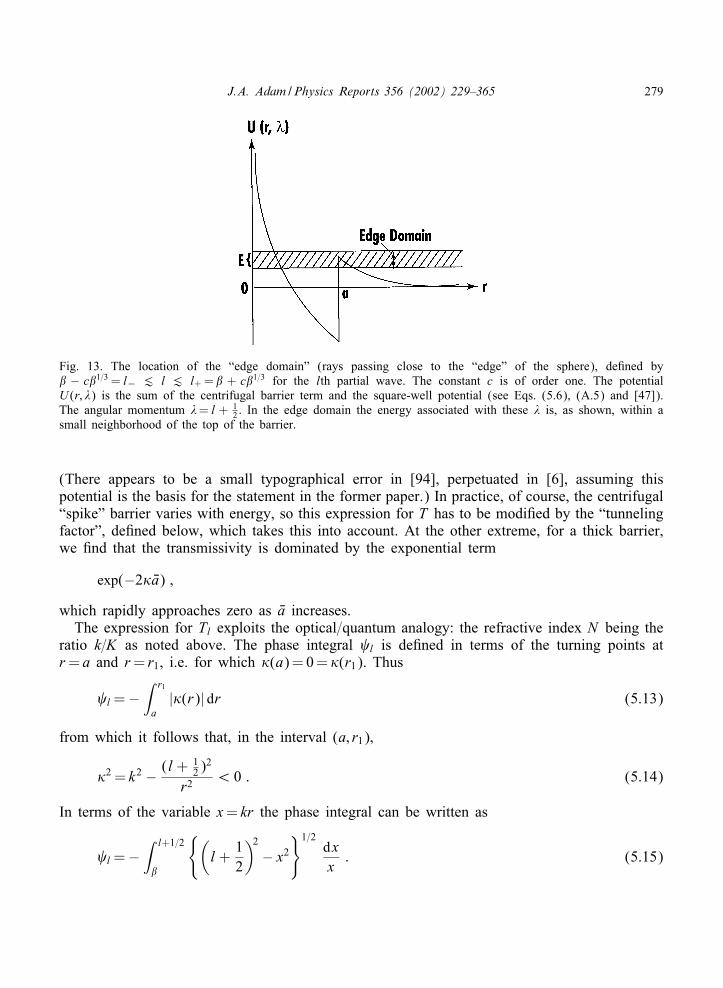
J.A. Adam /Physics Reports 356 (2002) 229–365 279
Fig. 13. The location of the “edge domain” (rays passing close to the “edge” of the sphere), deAned by − c1=3 = l− . l . l+ = + c1=3 for the lth partial wave. The constant c is of order one. The potentialU (r; �) is the sum of the centrifugal barrier term and the square-well potential (see Eqs. (5.6), (A.5) and [47]).The angular momentum �= l + 1
2 : In the edge domain the energy associated with these � is, as shown, within asmall neighborhood of the top of the barrier.
(There appears to be a small typographical error in [94], perpetuated in [6], assuming thispotential is the basis for the statement in the former paper.) In practice, of course, the centrifugal“spike” barrier varies with energy, so this expression for T has to be modiAed by the “tunnelingfactor”, deAned below, which takes this into account. At the other extreme, for a thick barrier,we And that the transmissivity is dominated by the exponential term
exp(−2Aa) ;
which rapidly approaches zero as a increases.The expression for Tl exploits the optical=quantum analogy: the refractive index N being the
ratio k=K as noted above. The phase integral l is deAned in terms of the turning points atr= a and r= r1, i.e. for which A(a)=0=A(r1). Thus
l =−∫ r1
a|A(r)| dr (5.13)
from which it follows that, in the interval (a; r1);
A2 = k2 − (l + 12)
2
r2¡ 0 : (5.14)
In terms of the variable x= kr the phase integral can be written as
l =−∫ l+1=2
{(l +
12
)2− x2
}1=2dxx
: (5.15)
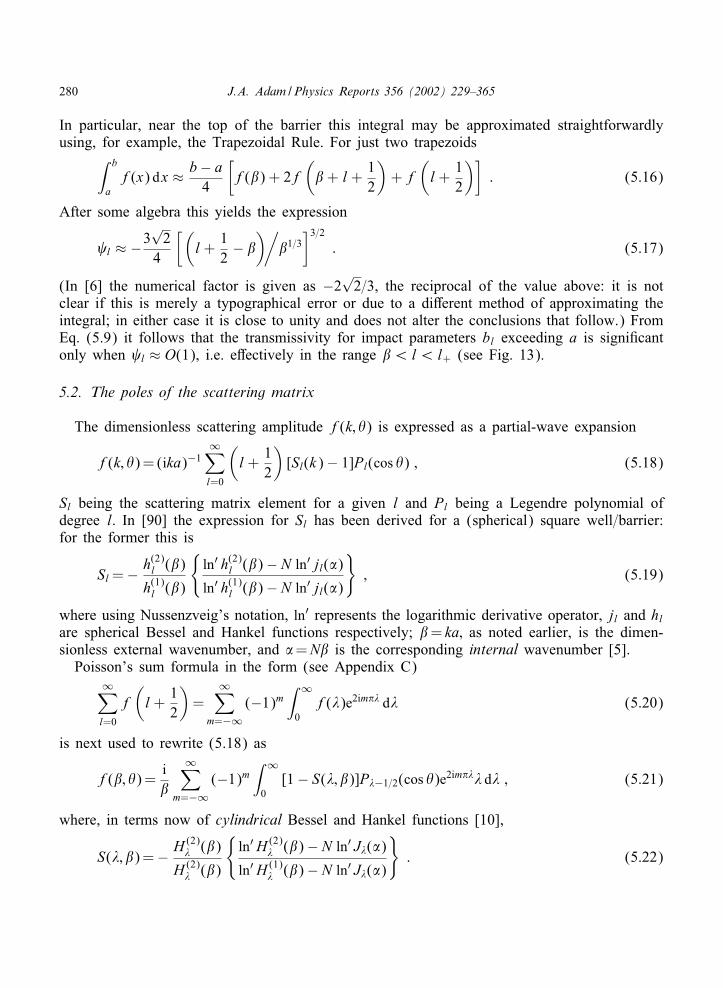
280 J.A. Adam /Physics Reports 356 (2002) 229–365
In particular, near the top of the barrier this integral may be approximated straightforwardlyusing, for example, the Trapezoidal Rule. For just two trapezoids∫ b
af(x) dx ≈ b− a
4
[f() + 2f
( + l +
12
)+ f
(l +
12
)]: (5.16)
After some algebra this yields the expression
l ≈ −3√
24
[(l +
12− )/
1=3]3=2
: (5.17)
(In [6] the numerical factor is given as −2√
2=3, the reciprocal of the value above: it is notclear if this is merely a typographical error or due to a di9erent method of approximating theintegral; in either case it is close to unity and does not alter the conclusions that follow.) FromEq. (5.9) it follows that the transmissivity for impact parameters bl exceeding a is signiAcantonly when l ≈ O(1), i.e. e9ectively in the range ¡l¡l+ (see Fig. 13).
5.2. The poles of the scattering matrix
The dimensionless scattering amplitude f(k; �) is expressed as a partial-wave expansion
f(k; �)= (ika)−1∞∑l=0
(l +
12
)[Sl(k)− 1]Pl(cos �) ; (5.18)
Sl being the scattering matrix element for a given l and Pl being a Legendre polynomial ofdegree l: In [90] the expression for Sl has been derived for a (spherical) square well=barrier:for the former this is
Sl =− h(2)l ()
h(1)l ()
{ln′ h(2)
l ()− N ln′ jl(5)
ln′ h(1)l ()− N ln′ jl(5)
}; (5.19)
where using Nussenzveig’s notation, ln′ represents the logarithmic derivative operator, jl and hlare spherical Bessel and Hankel functions respectively; = ka; as noted earlier, is the dimen-sionless external wavenumber, and 5=N is the corresponding internal wavenumber [5].
Poisson’s sum formula in the form (see Appendix C)∞∑l=0
f(l +
12
)=
∞∑m=−∞
(−1)m∫ ∞
0f(�)e2im�� d� (5.20)
is next used to rewrite (5.18) as
f(; �)=i
∞∑m=−∞
(−1)m∫ ∞
0[1− S(�; )]P�−1=2(cos �)e2im��� d� ; (5.21)
where, in terms now of cylindrical Bessel and Hankel functions [10],
S(�; )=− H (2)� ()
H (2)� ()
{ln′ H (2)
� ()− N ln′ J�(5)
ln′ H (1)� ()− N ln′ J�(5)
}: (5.22)
J.A. Adam /Physics Reports 356 (2002) 229–365 281
For Axed ; S(�; ) is a meromorphic function of the complex variable �, and in particularin what follows, it is the poles of this function that are of interest. They are deAned by thecondition
ln′ H (1)� ()=N ln′ J�(5) : (5.23)
In view of relationship (5.5) between the refractive index N and the square well depth −V0,these zeros may be identiAed with the Regge poles for a square potential well (N ¿ 1) or barrier(N ¡ 1). Several studies have been made of such poles for these potentials [96–100], both forN ¿ 1 and N ¡ 1: Nussenzveig [90] carried out a detailed investigation of the distribution ofsuch poles, particularly for the case of �1; some of this material is relevant to the rainbowscattering problem so a brief summary of the pertinent details will be provided here for N ¿ 1;but as is noted in [5], the physical interpretation is especially simple for N�1: This impliesthat 5��1, and renders it appropriate to use the asymptotic expansions for the Bessel andHankel functions. Physically, this corresponds to an optically dense material or an extremelydeep potential well (with, therefore, many energy levels). Mathematical details are provided in[98,99].
Under these approximations the complex �-plane is subdivided into seven regions, thoughthe Regge poles themselves can be associated with (i) broad resonances, (ii) narrow reso-nances and (iii) surface waves. Firstly, there exists a series of poles very close to the realaxis; optically they correspond to so-called free modes of vibration of a dielectric sphere. Theassociated high internal reTectivity (since N is large) and high centrifugal barrier (since l islarge) guarantee long lifetimes: the resonance appears when the pole is in close proximity toa physical value of �, i.e. �= l+ 1
2 : Quantum mechanically, a deep well surrounded by a highbarrier gives rise to sharp resonances. All these poles have their counterparts in the - (or k-)plane of course, from which the penetration factors exp(2 l) and resonance widths Fn can beestablished.
Another class of poles exists, this time not so close to the real �-axis, but with almostconstant imaginary part. These poles are associated with broad resonances above the top ofthe centrifugal barrier; again in the -plane the location of the corresponding poles providesinformation on the penetration factors and resonance widths. A third set of poles, this time near�=; have an extremely important physical interpretation, and to clarify this, we write downthe approximation for these, namely
�n ≈ +xnei�=3
(2=)1=3+
i(N 2 − 1)1=2
; (5.24)
where −xn is the nth zero of the Airy function Ai(z), i.e. Ai(−xn)=0: The Arst and secondterms occur in the expression for Regge poles for an impenetrable sphere [10,30], so the polesare related to surface waves. The second term contains a damping contribution which dependson the radius of curvature, and represents damping due to propagation along a curved surface.The Anal term represents damping due to refraction of the surface waves into the sphere, and byvirtue of the temporary assumption that N�1, this term is small, so the surface wave damping isdetermined primarily by geometry rather than refraction. For even larger values of |�| there arepoles which continue to be associated with surface waves by virtue of their similarity to those
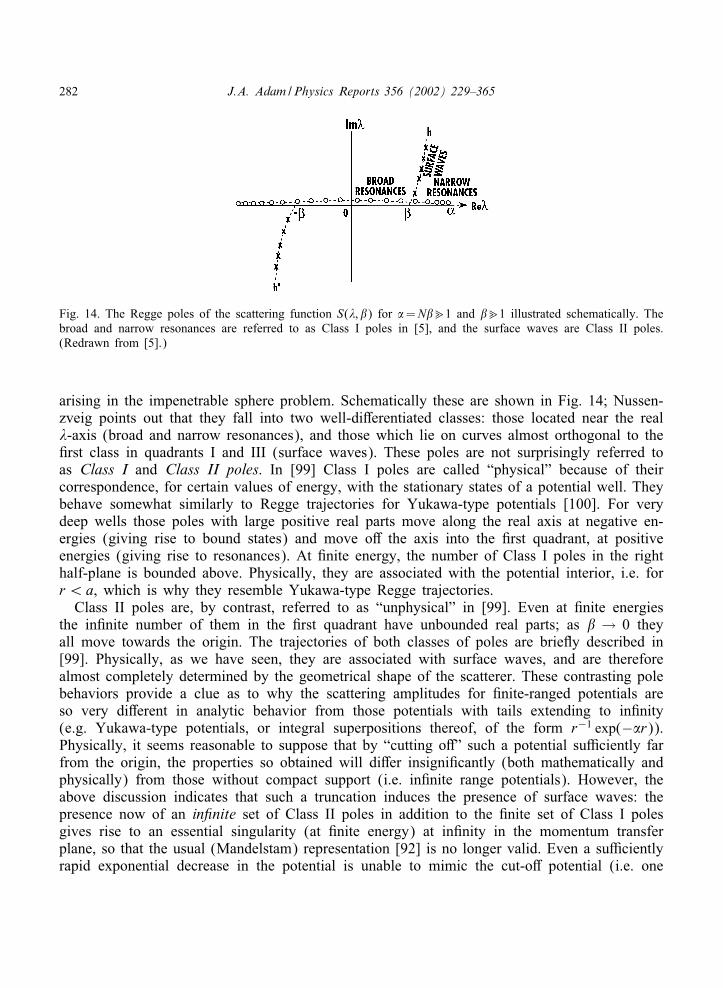
282 J.A. Adam /Physics Reports 356 (2002) 229–365
Fig. 14. The Regge poles of the scattering function S(�; ) for 5=N�1 and �1 illustrated schematically. Thebroad and narrow resonances are referred to as Class I poles in [5], and the surface waves are Class II poles.(Redrawn from [5].)
arising in the impenetrable sphere problem. Schematically these are shown in Fig. 14; Nussen-zveig points out that they fall into two well-di9erentiated classes: those located near the real�-axis (broad and narrow resonances), and those which lie on curves almost orthogonal to theArst class in quadrants I and III (surface waves). These poles are not surprisingly referred toas Class I and Class II poles. In [99] Class I poles are called “physical” because of theircorrespondence, for certain values of energy, with the stationary states of a potential well. Theybehave somewhat similarly to Regge trajectories for Yukawa-type potentials [100]. For verydeep wells those poles with large positive real parts move along the real axis at negative en-ergies (giving rise to bound states) and move o9 the axis into the Arst quadrant, at positiveenergies (giving rise to resonances). At Anite energy, the number of Class I poles in the righthalf-plane is bounded above. Physically, they are associated with the potential interior, i.e. forr¡a, which is why they resemble Yukawa-type Regge trajectories.
Class II poles are, by contrast, referred to as “unphysical” in [99]. Even at Anite energiesthe inAnite number of them in the Arst quadrant have unbounded real parts; as → 0 theyall move towards the origin. The trajectories of both classes of poles are brieTy described in[99]. Physically, as we have seen, they are associated with surface waves, and are thereforealmost completely determined by the geometrical shape of the scatterer. These contrasting polebehaviors provide a clue as to why the scattering amplitudes for Anite-ranged potentials areso very di9erent in analytic behavior from those potentials with tails extending to inAnity(e.g. Yukawa-type potentials, or integral superpositions thereof, of the form r−1 exp(−5r)).Physically, it seems reasonable to suppose that by “cutting o9” such a potential suYciently farfrom the origin, the properties so obtained will di9er insigniAcantly (both mathematically andphysically) from those without compact support (i.e. inAnite range potentials). However, theabove discussion indicates that such a truncation induces the presence of surface waves: thepresence now of an in?nite set of Class II poles in addition to the Anite set of Class I polesgives rise to an essential singularity (at Anite energy) at inAnity in the momentum transferplane, so that the usual (Mandelstam) representation [92] is no longer valid. Even a suYcientlyrapid exponential decrease in the potential is unable to mimic the cut-o9 potential (i.e. one
J.A. Adam /Physics Reports 356 (2002) 229–365 283
with compact support); the phrase ‘suYciently rapid’ implies a length scale much shorter thanthe wavelength under consideration, and this is not true at ‘suYciently high’ energies, whereascut-o9 potentials can support surface waves at arbitrarily high energy.
5.3. The Debye expansion
The Watson transformation is applicable to the problem of scattering by an impenetrablesphere; this is discussed in detail elsewhere [30]; see also [10] and Appendix C. However, inthe case of a transparent sphere, a large number of Regge poles lie in the neighborhood ofthe real axis, so if expression (5.21) for f(; �) were reduced to rapidly convergent contourintegrals plus a series of residues from the Regge poles, such a series would of necessityconverge very slowly (physically, the di9erence between the two cases arises because wavepenetration occurs in the transparent sphere). The number of such poles is of the order of(N − 1), as may be seen from Eq. (2:37) in [6], which means that the minimum numberof residue terms required is at least of the same order as the number of terms needed inthe original partial-wave series (a large number of such waves can be near resonance at highfrequencies). In [33], the contour integrals were evaluated by the saddle point method, thecontributions from which correspond to those arising from geometrical optics, at least to a Arstapproximation. This is perfectly acceptable for the impenetrable sphere, for which only directreTection occurs, but in the present case an incident ray is partially reTected and partiallytransmitted, the latter in turn being partially (internally) reTected and partially transmitted, andso on. Thus an inAnite series of multiple internal reTections (or interactions with the surface)corresponds to an inAnite number of saddle points, which must be appropriately superimposedto enable the external solution to be constructed. The Debye series is just this: a representationof the scattering problem in terms of surface interactions; Debye adopted this method for acircular cylinder [101], and later van der Pol and Bremmer applied it to the sphere [30,31]. Thisis done by means of a related but Actitious problem; i.e. by regarding the surface r= a as aninterface between two unbounded homogeneous media and matching the solutions to the (radial)equation to determine the internal and external spherical reTection and transmission coeYcients.The interaction of an incoming spherical wave with the sphere is then described in terms of asequence of surface interactions (partial reTections and transmissions) with interior propagationoccurring in an alternate fashion. In particular, the external and internal spherical reTectioncoeYcients R22 and R11 are given by Eqs. (5.25) and (5.26) for the scalar scattering problem(for the full electromagnetic problem there is a corresponding coeYcient for each polarization;see [10,102] for details):
R22(�; )=−(
ln′ H (2)� ()− N ln′ H (2)
� (5)
ln′ H (1)� ()− N ln′ H (2)
� (5)
)(5.25)
and
R11(�; )=−(
ln′ H (1)� ()− N ln ′H (1)
� (5)
ln′ H (1)� ()− N ln′ H (2)
� (5)
): (5.26)
284 J.A. Adam /Physics Reports 356 (2002) 229–365
From conservation of energy (or probability in the quantum–mechanical context) the followingrelationships hold:
|R22(�; )|2 +
∣∣∣∣∣H(2)� ()
H (2)� (5)
T21(�; )
∣∣∣∣∣2
=1 (5.27)
and
|R11(�; )|2 +
∣∣∣∣∣H(1)� (5)
H (1)� ()
T12(�; )
∣∣∣∣∣2
=1 ; (5.28)
where Tij is the spherical transmission coeYcient from medium i to medium j (i; j=1; 2; theinterior and exterior of the sphere are denoted by indices 1 and 2, respectively). In the limit asthe radius a of the sphere tends to inAnity, the above four coeYcients reduce to the standardFresnel coeYcients for reTection and transmission for a plane interface at normal incidence, i.e.
R11 → N − 1N + 1
; T12 → 2NN + 1
(5.29)
and R22 =− R11; T21 =T12:The scattering function S(�; ) (Eq. (5.22)) is to be expressed in terms of surface interactions;
in order to accomplish this the external reTection coeYcient R22 is subtracted from S; after somerearrangement this can be written in terms of the quantity.
G(�; )=H (1)
� (5)
H (2)� (5)
R11(�; ) (5.30)
as
S(�; )=H (2)
� ()
H (1)� ()
R22(�; ) + T21(�; )T12(�; )
H (1)� (5)
H (2)� (5)
∞∑p=1
[G(�; )]p−1
: (5.31)
This is the celebrated Debye expansion, arrived at by expanding the expression [1− G(�; )]−1
as an inAnite geometric series. The Arst term inside the parentheses represents direct reTectionfrom the surface; the pth term represents transmission into the sphere (from the term T21)subsequently “bouncing” back and forth between r= a and 0 a total of p times (from the ratioof Hankel functions preceding the summation), with p−1 internal reTections at the surface (viathe R11 term in G; the case p=1 corresponds to direct transmission). The Anal factor in thesecond term, T12, corresponds to transmission to the outside medium. The multiplicative factoroutside the parentheses is phase term due to the surface interaction taking place at r= a ratherthan r=0: The origin behaves as a perfectly reTecting “boundary” because of the regularity ofthe wavefunction there. In summary, therefore, the pth term of the Debye expansion representsthe e;ect of p + 1 surface interactions.
Regarding convergence of the expansion, it follows from Eqs. (5.28) and (5.30) for real �that
|G(�; )|= |R11(�; )|¡ 1 :

J.A. Adam /Physics Reports 356 (2002) 229–365 285
Nussenzveig [6] also shows that
lim� →±∞
|G(�; )|=1 ; (5.32)
so that any improper integrals for �∈ (0;∞) must be interpreted in the limiting sense of�∈ (0; $); $ → ∞: In this spirit we may write
f(; �)=f0(; �) +∞∑
p=1
fp(; �) ; (5.33)
where
f0(; �)=i
∞∑m=−∞
(−1)m∫ ∞
0
[1− H (2)
� ()
H (1)� ()
R22
]P�−1=2(cos �) exp(2im��)� d� (5.34)
and
fp(; �)=− i
∞∑m=−∞
(−1)m∫ ∞
0U (�; )[G(�; )]p−1P�−1=2(cos �) exp(2im��)� d� (5.35)
for p¿ 1: In this last expression
U (�; )=T21(�; )H (1)
� (5)
H (2)� (5)
H (2)� ()
H (1)� ()
T12(�; )=U (−�; ) : (5.36)
In practice, contributions to the integrals in (5.33) for large values of � become vanishinglysmall, so the e9ect of condition (5.32) is negligible. Alternative but equivalent representationsto f(; �) are also possible (see [5] for details).
While convergence of the Debye expansion is a fundamental mathematical property, onceestablished it is necessary to ask the practical question: how rapid is the convergence? Theearlier expression (5.21) for f(; �) involves a slowly converging residue series because of theexistence of many Regge poles close to the real axis. What happens when the modiAed Watsontransformation is applied now, i.e. how are the poles for each term distributed in the complex-�plane? A distinct but related question concerns how fast the Debye expansion itself converges.
The poles for the Debye expansion di9er from the Regge poles associated with expression(5.23); they are deAned by
ln′ H (1)� ()=N ln′ H (2)
� (5) (5.37)
corresponding to the replacement of standing waves (Regge poles) by travelling waves (Debyeinteractions). Interestingly, the locations of the poles are the same for each term, but their ordervaries: they are of order p+ 1 for the pth term (p=0; 1; 2; : : :). There are now two classes ofpoles to consider, each being symmetrically located with respect to the origin, denoted in [5]by �n and �′n respectively. In the right half-plane, for N | − 1|�1=3; using earlier notation
�n ≈ + ei�=3(xn=6)− i=M (5.38)
286 J.A. Adam /Physics Reports 356 (2002) 229–365
for N ¿ 1; (the only situation which concerns us in this paper). Similarly,
�′n ≈ 5 + e−i�=3N 1=3(xn=6) + N=M (5.39)
for N ¿ 1:The set {�n} di9ers little from that corresponding to the impenetrable sphere problem, so it
is closely associated with surface waves. This is actually the case for the set {�′n} as well: the�′n lie in the fourth quadrant, and arise from the Debye expansion; however, for N ¿ 1 theircontributions are negligible (which is not the case for N ¡ 1) and so they will not be discussedfurther here.
In general, when the modiAed Watson transformation is applied to each term in the Debyeexpansion, the dominant contributions to the asymptotic behavior of each term will be fromsaddle points and residue series, the former corresponding to rays in geometrical optics. Thus foreach term there is a Anite number of saddle points, though this number does increase for eachsuccessive term. The residue-series terms converge rapidly (the imaginary part of �n increasesrapidly with n), and so overall a rapidly convergent asymptotic expansion for each term of theDebye expansion can be obtained.
Returning to the question of convergence of the Debye series itself, the saddle-point con-tributions converge at a rate determined by the damping produced at each internal reTection.This in turn is determined by the Fresnel reTection coeYcient at the interface, and that dependson the impact parameter and the value of N: For most directions (excluding the cases N�1and N�1) this coeYcient is small and as a consequence the Debye series converges quiterapidly. The convergence rate will be enhanced if the scattering sphere is not transparent, i.e.if absorption occurs in the interior; mathematically this can be accommodated by allowing Nto be a complex number.
Van de Hulst [7] has estimated that for water droplets (N ≈ 1:33 for orange light) more than98:5% of the total intensity of incident radiation is accounted for by the rays 1′; 2′ and 3′ inFig. 1(c); these correspond to the Arst three terms in the Debye expansion. Thus the remainder,less than 1.5%, must be distributed among the higher-order terms and the contributions from theresidue series. This is not to say, however, that they do not contribute signiAcantly; they can beconcentrated within narrow angular domains about certain directions (see Section 5.4 below).Indeed, the phenomenon of the “glory” (see Section 3 and [47]) is a consequence of theseresidue-series contributions dominating the geometrical ray contributions in a particular angularregion. These contributions in general converge considerably more slowly than their saddle-pointcounterparts. This can be appreciated on physical grounds by considering what happens to theincident ray as the impact parameter increases. Under these circumstances the reTection coeY-cient increases towards unity (total reTection) as glancing incidence (for N ¿ 1) is approached.At glancing incidence these rays are of course totally reTected within the approximation ofgeometrical optics, but these are precisely the limiting rays responsible for the excitation ofsurface waves. The consequence of high reTectivity inevitably implies slow convergence ofthese surface-wave contributions.
In [5], Nussenzveig examined in detail the Arst two terms of the Debye expansion (and in [6]the third term and e9ects associated with higher-order terms were discussed in connection withboth the optical rainbow and glory). The Arst two terms are associated respectively with direct
J.A. Adam /Physics Reports 356 (2002) 229–365 287
reTection from the surface of the scatterer and direct transmission (with no internal reTection),consistent with the physical interpretation of the Debye series. The asymptotic expansions werecarried out up to (but not including) correction terms of order (ka)−2. The behavior of theArst term is similar to that found for the impenetrable sphere problem, exhibiting (for N ¿ 1)a forward di9raction peak, a geometrical reTection (or lit) region, and a transition region inwhich the scattering amplitude is expressible in terms of generalizations of Fock functions (seeEq. (4:67) in [5] and Appendix 2), the latter being deAned in [33] as
F(1)=∫ ∞
0
ei1x
Ai(xei�=3)dx +
∫ ∞
0
e−i1x
Ai(xe−i�=3)dx : (5.40)
The second term gives rise to a lit region, a shadow region and again, a Fock-type transitionregion. By a process termed critical refraction, surface waves are able to take “shortcuts” acrossthe sphere. The application of the modiAed Watson transform to the third term in the Debyeexpansion of the scattering amplitude is examined by Nussenzveig in [6], along with the e9ectof higher-order terms. It is this term which is associated with the phenomena of the rainbowand the glory.
The theory for the Arst two terms is uniformly valid for all N ¿ 1; this is not the casefor the third term however. It transpires that there are Ave di9erent ranges of the refractiveindex to be considered: each of them requires a separate treatment [6,34]. These subdivisionscan be found directly from geometrical optics considerations; corresponding to di9erent valuesof N there are di9erent angular regions characterized by the number of rays—0; 1; 2 or 3—ina particular direction within that region. The only range of signiAcance here is 1¡N ¡
√2;
the refractive index of water for the optical spectrum falls within this range, and from nowon all statements made pertain to it. From a consideration of geometrical optics, there arethree di9erent angular regions to examine: (i) a 0-ray (shadow) region located near the for-ward region, 06 �¡�R; (ii) a 1-ray region near the backward direction, �L ¡�6�; where asshown below, �L =4 arccos(1=N ) and (iii) a 2-ray region between them, �R ¡�¡�L: However,the presence of (non-geometrical optics) transition regions leads to a total of six regions toexamine for �∈ (0; �); the three additional regions arise because of di9raction e9ects at theboundaries between the above three regions. The transition region near �=� corresponds to the“glory” region, and the 2-ray=0-ray (light=shadow or caustic) transition region corresponds tothe “rainbow” region. There is a penumbra region around the 1-ray=2-ray boundary.
The so-called “normal” regions can be described as follows. The 1-ray region contains thesingle geometrical optics contribution plus surface waves excited at the 2-ray=1-ray shadowboundary; these are associated with di9racted rays that take two “shortcuts” across the scatteringsphere. This 2-ray=1-ray transition region corresponds to one of the normal “Fock-type” regions.The 2-ray region contains two real saddle points (one for each ray direction in this region) whichbecome complex in the 0-ray (shadow) region; here the scattering amplitude cannot be reducedto a pure residue series.
The rainbow light=shadow transition region is associated physically with the conTuence ofa pair of geometrical rays and their transformation into “complex rays”; mathematically thiscorresponds to a pair of real saddle points merging into a complex saddle point. Then theproblem is to And the asymptotic expansion of an integral having two saddle points that movetowards or away from each other. The generalization of the standard saddle-point technique to
288 J.A. Adam /Physics Reports 356 (2002) 229–365
include such problems was made by Chester et al. [72] and using their method, Nussenzveigwas able to And a uniform asymptotic expansion of the scattering amplitude which was validthroughout the rainbow region, and which matched smoothly onto results for neighboring re-gions (see Appendix D). The lowest order approximation in this expansion turns out to be thecelebrated Airy approximation which, despite several attempts to improve upon it, was the bestapproximate treatment prior to the analyses of Nussenzveig and coworkers. However, Airy’stheory had a limited range of applicability as a result of its underlying assumptions; by con-trast the uniform expansion is valid over a much larger range. This new approach also enablesa quantitative theory of the glory—a strong enhancement of scattering in the near-backwarddirection, as noted in Section 3—to be developed. The intensity predicted by geometrical op-tics is not nearly suYcient to account for this e9ect. In 1947, Van de Hulst conjectured thatthe glory is due to surface waves that make two shortcuts across the sphere ([50], see also[7]), but no quantitative analysis had been provided. Nussenzveig used the modiAed Watsontransform to advantage in the backward scattering direction, and evaluated the residue-seriescontributions there, showing that they are indeed capable of accounting for the enhancement inthe backward intensity, thus conArming Van de Hulst’s conjecture (as far as the third term ofthe Debye series is concerned; but many other terms contribute to the glory, as summarized inSection 5.7 below). The enhancement arises from the focusing of di9racted rays on the axiswhich compensates for the exponential damping over the surface of the sphere, and illustratesthe phenomenon of “Regge-pole dominance” of the scattering amplitude.
Nevertheless, the “third term” theory, highly successful as it is, is not able to satisfactorilyaccount for the backward-scattered intensity as a function of ; it transpires that contributionsfrom higher-order terms in the Debye expansion are necessary to explain the results obtainedby numerical summation of the partial-wave series (and note that the fourth term in the Debyeexpansion corresponds to the secondary rainbow). As noted in Section 3, Bryant and Cox [54]found a very complicated Ane structure consisting of a quasiperiodic pattern with prominent butirregular peaks, and it is this type of behavior that requires higher-order terms to be invoked.Despite some mathematically technical diYculties, it was shown that the quasiperiodic Anestructure could be accounted for in this way, and also resonance e9ects predicted. Furthermore,the same e9ects can be shown to be responsible for the “ripple” in the total cross section forN ¿ 1 (see [10,88,89] and Section 5.6 for more details).
Explicitly, the third term in the Debye expansion is, from (5.35),
f2(; �)=− i
∞∑m=−∞
(−1)m∫ ∞
0U (�; )G(�; )P�−1=2(cos �) exp(2im��)�d� : (5.41)
After some rearrangement, and a shift in the path of integration to the above real axis, this canbe written as
f2(; �)=− i2
∫ ∞+ij
−∞−ijU (�; )G(�; )P�−1=2(cos �) exp(i��)
�cos��
d� ; (5.42)
where H¿ 0: Furthermore, this integral can be decomposed into
f2(; �)=f+2;0 + f2; r =f−
2;0 − f2; r ; (5.43)
J.A. Adam /Physics Reports 356 (2002) 229–365 289
where
f±2;0(; �)=± i
∫ ∞∓ij
−∞±ijGUQ(2)
�−1=2(cos �)� d� (5.44)
and
f2; r(; �)=12
∫ ∞+ij
−∞−ijGU exp(2i��)
� d�cos��
: (5.45)
In expression (5.44), Q(2)�−1=2 is a Legendre function of the second kind. Details of these manip-
ulations can be found in [33,6]. It can also be shown from the nature of the integrand in (5.44)that there is always some neighborhood of the imaginary axis where that integrand diverges toinAnity. Since this is true for any value of �, it follows that there is no domain of �-values inwhich f±
2;0 (and hence f2(; �)) can be reduced to a pure residue series.
5.4. Geometrical optics rBegimes
As previously noted, the third term of the Debye expansion corresponds to rays that aretransmitted out of the transparent sphere after one internal reTection. There are in fact threepossible types of ray trajectories depending on the value of the refractive index N . The oneof concern here is for N in the domain (1; 2); in fact it is the subdomain (1;
√2) that will be
examined below. The other domains are of course (0; 1) and (2;∞); again, further subdivisionsoccur, so that there are in total ?ve subdomains:
(0; 1); (1;√
2); (√
2; [6√
3− 8]1=2); ([6√
3− 8]1=2; 2) and (2;∞) :
The mathematics based on ray theory has been discussed earlier so we merely summarize ithere. In terms of the angles of incidence, refraction and deTection (or scattering), �i; �r and �(= i; r; and Dk , respectively, in Section 1.3)
sin �i =N sin �r; 06 �i; �r6�=2; 06 �6�
and
�=2(�i − 2�r) + � : (5.46)
For the deTection angle to be no greater than � radians it is necessary that ,= �i − 2�r6 0;the limiting angle of incidence �a
i such that ,=0 satisAes the implicit condition
�ai =2 arcsin
(sin �a
i
N
)(5.47)
or explicitly
cos �ai =
12(N
2 − 2) (5.48)

290 J.A. Adam /Physics Reports 356 (2002) 229–365
Fig. 15. A schematic representation of the six angular regions associated with both rainbow and glory scatteringfrom a spherical water droplet. The glory, rainbow and 2-ray=1-ray transition region are greatly exaggerated forclarity. The angular size of these regions are noted (see text for details). This is valid for 1¡N ¡
√2: The rainbow
angle is �R and �L is the 2-ray=1-ray boundary angle. (Redrawn from [6].)
(excluding the zero impact parameter case cos �ai =1). Since �i ∈ [0; �=2] it follows that such an
angle �ai only exists for N ∈ [
√2; 2]: In terms of ,, it can be seen that
d,dN
=2 sin �i=N 2√
1− (sin �i=N )2¿ 0 ;
i.e. , is an increasing function of N . Since ,=0 for N =√
2, it follows that the range ofinterest here corresponds to ,¡ 0, i.e. N ∈ (1;
√2): Note also that the limiting incident ray is
�i =�2; �r =arcsin
1N
= �l ; (5.49)
the corresponding scattering angle is
�L =2�− 4 arcsin1N
=4 arccos1N
: (5.50)
Finally, as noted in Section 1.3, the rainbow angle (the minimum value of the scattering angle)is, in the present notation,
�R =� + 2�i;R − 4 arcsin(
sin �i;R
N
)
where
�i;R =arccos(N 2 − 1
3
)1=2:
The angle �L is a 1-ray=2-ray shadow boundary; the rainbow appears around the angle �R, whichis a 2-ray=0-ray shadow boundary (see Fig. 15).
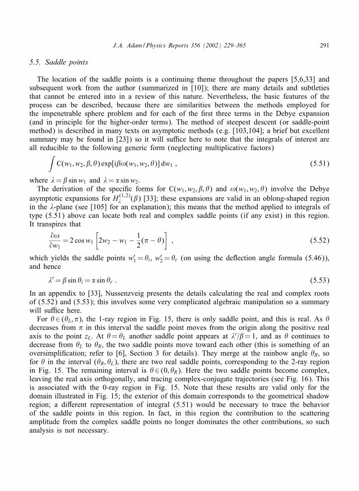
J.A. Adam /Physics Reports 356 (2002) 229–365 291
5.5. Saddle points
The location of the saddle points is a continuing theme throughout the papers [5,6,33] andsubsequent work from the author (summarized in [10]); there are many details and subtletiesthat cannot be entered into in a review of this nature. Nevertheless, the basic features of theprocess can be described, because there are similarities between the methods employed forthe impenetrable sphere problem and for each of the Arst three terms in the Debye expansion(and in principle for the higher-order terms). The method of steepest descent (or saddle-pointmethod) is described in many texts on asymptotic methods (e.g. [103,104]; a brief but excellentsummary may be found in [23]) so it will suYce here to note that the integrals of interest areall reducible to the following generic form (neglecting multiplicative factors)∫
C(w1; w2; ; �) exp[i!(w1; w2; �)] dw1 ; (5.51)
where �= sinw1 and �= 5 sinw2:The derivation of the speciAc forms for C(w1; w2; ; �) and !(w1; w2; �) involve the Debye
asymptotic expansions for H (1;2)� () [33]; these expansions are valid in an oblong-shaped region
in the �-plane (see [105] for an explanation); this means that the method applied to integrals oftype (5.51) above can locate both real and complex saddle points (if any exist) in this region.It transpires that
9!9w1
=2 cosw1
[2w2 − w1 − 1
2(�− �)
]; (5.52)
which yields the saddle points w′1 = �i; w′
2 = �r (on using the deTection angle formula (5.46)),and hence
�′ = sin �i = 5 sin �r : (5.53)
In an appendix to [33], Nussenzveig presents the details calculating the real and complex rootsof (5.52) and (5.53); this involves some very complicated algebraic manipulation so a summarywill suYce here.
For �∈ (�L; �); the 1-ray region in Fig. 15, there is only saddle point, and this is real. As �decreases from � in this interval the saddle point moves from the origin along the positive realaxis to the point zL: At �= �L another saddle point appears at �′==1, and as � continues todecrease from �L to �R, the two saddle points move toward each other (this is something of anoversimpliAcation; refer to [6], Section 3 for details). They merge at the rainbow angle �R; sofor � in the interval (�R; �L); there are two real saddle points, corresponding to the 2-ray regionin Fig. 15. The remaining interval is �∈ (0; �R): Here the two saddle points become complex,leaving the real axis orthogonally, and tracing complex-conjugate trajectories (see Fig. 16). Thisis associated with the 0-ray region in Fig. 15. Note that these results are valid only for thedomain illustrated in Fig. 15; the exterior of this domain corresponds to the geometrical shadowregion; a di9erent representation of integral (5.51) would be necessary to trace the behaviorof the saddle points in this region. In fact, in this region the contribution to the scatteringamplitude from the complex saddle points no longer dominates the other contributions, so suchanalysis is not necessary.
292 J.A. Adam /Physics Reports 356 (2002) 229–365
Fig. 16. The coalescence of two real saddle points in the complex �-plane as the rainbow angle �R is approachedfrom below (i.e. from the lit side). At �R the points collide and subsequently move away from each other alongcomplex-conjugate directions as � increases away from �R into the shadow region. It is the lower complex saddlepoint that contributes to the wave Aeld in this region.
It has been noted already that there is a total of six angular regions in (0; �) of interest inthe full scattering problem for 1¡N ¡
√2; the regions [0; �R); (�R; �L) and (�L; �] discussed
above, together with their transition regions and a transition region near the backward direction(the glory region). We defer discussion of this and the rainbow region and brieTy discuss thenature of the remaining four so-called “normal” regions.
5.5.1. The 1-ray regionThis is the region
�− �L�6=(2=)1=3; �− ��−1=2 ;
where the latter restriction is to enable the asymptotic expansion for Q(2)�−1=2(cos �) to be utilized
in (5.44), leading to the integral representation (5.51). The path of steepest descent crosses thereal axis at the (unique) saddle point at an angle of �=4, as it passes from the third quadrantthrough the fourth to the Arst quadrant. The third term in the Debye expansion (referred to hereas f2 for brevity) is dominated by the WKB approximation, representing the contribution fromone geometrical ray (transmitted after one internal reTection; see Fig. 1(a)).
5.5.2. The 2-ray regionThis is the region
�L − ��6; �− �R�62=M ;
where the second restriction is related to the condition for validity of the Debye asymptotic ex-pansion. Essentially, it requires that the “range” of the (now two) saddle points [103] be muchsmaller than their separation distance (see Appendix D). In this region the path of steepest
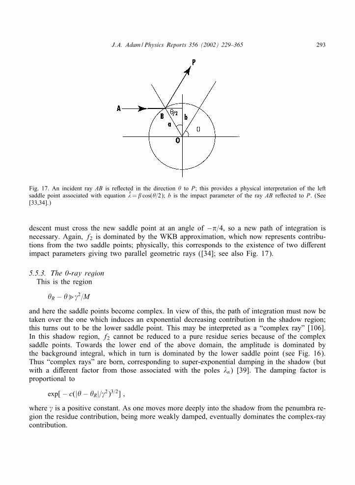
J.A. Adam /Physics Reports 356 (2002) 229–365 293
Fig. 17. An incident ray AB is reTected in the direction � to P; this provides a physical interpretation of the leftsaddle point associated with equation �= cos(�=2); b is the impact parameter of the ray AB reTected to P. (See[33,34].)
descent must cross the new saddle point at an angle of −�=4, so a new path of integration isnecessary. Again, f2 is dominated by the WKB approximation, which now represents contribu-tions from the two saddle points; physically, this corresponds to the existence of two di9erentimpact parameters giving two parallel geometric rays ([34]; see also Fig. 17).
5.5.3. The 0-ray regionThis is the region
�R − ��62=M
and here the saddle points become complex. In view of this, the path of integration must now betaken over the one which induces an exponential decreasing contribution in the shadow region;this turns out to be the lower saddle point. This may be interpreted as a “complex ray” [106].In this shadow region, f2 cannot be reduced to a pure residue series because of the complexsaddle points. Towards the lower end of the above domain, the amplitude is dominated bythe background integral, which in turn is dominated by the lower saddle point (see Fig. 16).Thus “complex rays” are born, corresponding to super-exponential damping in the shadow (butwith a di9erent factor from those associated with the poles �n) [39]. The damping factor isproportional to
exp[− c(|�− �R|=62)3=2] ;where 6 is a positive constant. As one moves more deeply into the shadow from the penumbra re-gion the residue contribution, being more weakly damped, eventually dominates the complex-raycontribution.
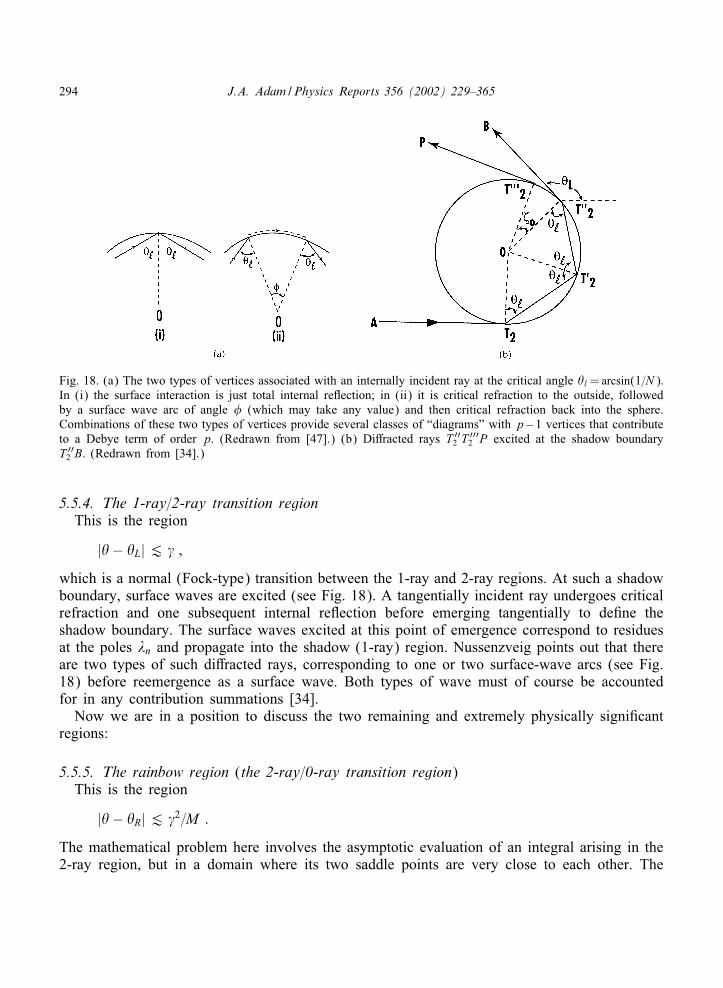
294 J.A. Adam /Physics Reports 356 (2002) 229–365
Fig. 18. (a) The two types of vertices associated with an internally incident ray at the critical angle �l =arcsin(1=N ):In (i) the surface interaction is just total internal reTection; in (ii) it is critical refraction to the outside, followedby a surface wave arc of angle , (which may take any value) and then critical refraction back into the sphere.Combinations of these two types of vertices provide several classes of “diagrams” with p−1 vertices that contributeto a Debye term of order p. (Redrawn from [47].) (b) Di9racted rays T ′′
2 T ′′′2 P excited at the shadow boundary
T ′′2 B. (Redrawn from [34].)
5.5.4. The 1-ray=2-ray transition regionThis is the region
|�− �L|. 6 ;
which is a normal (Fock-type) transition between the 1-ray and 2-ray regions. At such a shadowboundary, surface waves are excited (see Fig. 18). A tangentially incident ray undergoes criticalrefraction and one subsequent internal reTection before emerging tangentially to deAne theshadow boundary. The surface waves excited at this point of emergence correspond to residuesat the poles �n and propagate into the shadow (1-ray) region. Nussenzveig points out that thereare two types of such di9racted rays, corresponding to one or two surface-wave arcs (see Fig.18) before reemergence as a surface wave. Both types of wave must of course be accountedfor in any contribution summations [34].
Now we are in a position to discuss the two remaining and extremely physically signiAcantregions:
5.5.5. The rainbow region (the 2-ray=0-ray transition region)This is the region
|�− �R|. 62=M :
The mathematical problem here involves the asymptotic evaluation of an integral arising in the2-ray region, but in a domain where its two saddle points are very close to each other. The
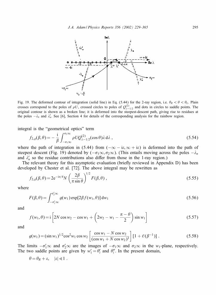
J.A. Adam /Physics Reports 356 (2002) 229–365 295
Fig. 19. The deformed contour of integration (solid line) in Eq. (5.44) for the 2-ray region, i.e. �R ¡�¡�L. Plaincrosses correspond to the poles of GU , crossed circles to poles of Q(2)
�−1=2 and dots in circles to saddle points. Theoriginal contour is shown as a broken line; it is deformed into the steepest-descent path, giving rise to residues atthe poles −�n and �′n: See [6], Section 4 for details of the corresponding analysis for the rainbow region.
integral is the “geometrical optics” term
f2; g(; �)=− i
∫ /2∞
−/1∞GUQ(2)
�−1=2(cos �)� d� ; (5.54)
where the path of integration in (5.44) from (−∞ − iH;∞ + iH) is deformed into the path ofsteepest descent (Fig. 19) denoted by (−/1∞; /2∞): (This entails moving across the poles −�nand �′n so the residue contributions also di9er from those in the 1-ray region.)
The relevant theory for this asymptotic evaluation (brieTy reviewed in Appendix D) has beendeveloped by Chester et al. [72]. The above integral may be rewritten as
f2; g(; �)=2e−i�=4N(
2� sin �
)1=2F(; �) ; (5.55)
where
F(; �)=∫ /′2∞
−/′1∞g(w1) exp[2f(w1; �)] dw1 (5.56)
and
f(w1; �)= i[2N cosw2 − cosw1 +
(2w2 − w1 − �− �
2
)sinw1
](5.57)
and
g(w1)= (sinw1)1=2cos2w1 cosw2
[cosw1 − N cosw2
(cosw1 + N cosw2)3
][1 + O(−1)] : (5.58)
The limits −/′1∞ and /′
2∞ are the images of −/1∞ and /2∞ in the w1-plane, respectively.The two saddle points are given by w′
1 = �′i and �′′i : In the present domain,
�= �R + H; |H|�1 :
296 J.A. Adam /Physics Reports 356 (2002) 229–365
If we take H¿ 0 initially, then the saddle points are real. To illustrate the complexity of thecalculations, note that after a great deal of analysis it can be shown that [6]
f2; g(; �)= 4ei�=4N( �sin �
)1=2(2)1=6 exp[2A(j)]{p0(j)Ai[(2)2=3>(j)] ;
− q0(j)(2)1=3
Ai′[(2)2=3>(j)]}[1 + O(−1)] ; (5.59)
where
A(H)= i[N (cos �′r + cos �′′r )− 12(cos �
′i + cos �′′i )] ; (5.60)
23[>(H)]
3=2 = i[N (cos �′r − cos �′′r )− 12(cos �
′i − cos �′′i )] ; (5.61)
p0; q0 =e−i�=4
4N>±1=4
[(sin �′′i
2 cos �′′i − N cos �′′r
)1=2(2N cos �′′i cos �′′r )
3=2 (cos �′′i − N cos �′′r )(cos �′′i + N cos �′′r )3
±(
sin �′iN cos �′r − 2 cos �′i
)1=2(2N cos �′i cos �
′r)
3=2 (cos �′i − N cos �′r)(cos �′i + N cos �′r)3
][1 + O(−1)]
(5.62)
and the ± signs correspond to p0 and q0; respectively. Also recall that �′1 and �′′1 are the saddlepoints. The expressions for A(j) and >(j) correspond to half the sum and half the di9erenceof the optical paths through the sphere, respectively. Very close to the rainbow angle, i.e. for|j|�1, the approximations for the above quantities may be substituted into the expression forf2; g(; �) to yield a still very complicated expression (see [6] for details); the result is a goodapproximation for |j|�6, containing as it does, the rainbow region. The dominant contributionto the third Debye term for the scattering amplitude Sj2(; �) turns out to be proportional to7=6: The above approximation can still be employed over part of the 2-ray region, where theAiry functions may be replaced by their asymptotic expansions for negative arguments, whichwe will not state here. The resulting expression is oscillatory (containing a sinusoidal term)and is associated with the interference between the two geometrical ray contributions, givingrise to the supernumerary bows referred to in the introduction. Other expressions, valid forstill larger scattering angles in the 2-ray region, may be derived which coincide exactly withthe results obtained by the saddle-point method, so the Chester–Friedman–Ursell method leadsto a uniform asymptotic expansion, matching smoothly the result obtained by the saddle-pointmethod in its domain of validity.
In the 0-ray region, within the domain 62=M�|j|�−1=2, j¡ 0 so the asymptotic expansionsfor Airy functions with positive arguments may now be used, resulting in an expression forthe complex-ray contribution (described above) and giving rise to Alexander’s dark band be-tween the primary and secondary bows. Further away from the rainbow angle, the residue-seriescontributions dominate the amplitude in the deep shadow region.
J.A. Adam /Physics Reports 356 (2002) 229–365 297
Airy’s approximation may be recovered from the |j|�1 version of Eq. (5.59) for f2; g(; �),as expected; this is
f(Airy)2; g (; �)=−16
27(3)7=12
(2)1=3e−i�=4 N 2(N 2 − 1)1=4
(8 + N 2)1=2(4− N 2)2=31=6
×exp{
i√3[6(N 2 − 1)1=2 + (4− N 2)1=2(�− �R)]
}
×Ai
[−(N 2 − 1)1=2
(4− N 2)1=6
(23
)2=3(�− �R)
]: (5.63)
Van de Hulst [7] claims that this approximation is a useful quantitative theory only for¿ 5000 (or drops of radius greater than about 0:5 mm) and |j|¡ 0:5◦; although Huygen’sprinciple may still be applied for ¿ 2000, “a quantitative theory of the rainbow for the entiregap 30¡¡ 2000 is still lacking”. The above contributions from Nussenzveig and coworkersbridge this gap and more; indeed, to quote from [10, Section 8:6],
the CAM theory bridges the gap between short-wavelength and long-wavelength scattering,remaining applicable all the way down to ∼ 1 : : : For ¿ 100, the accuracy of the CAMapproximation is better than 1 ppm, i.e. it becomes, for all practical purposes, more accuratethan the ‘exact’ partial-wave expansion!
(For further comments on accuracy see Section 5.7 below). For of the order of a fewhundred, within the domain |j|�6, the corrections to Airy’s theory can attain several percent;this increases with deviation from the rainbow angle.
5.6. The glory
The post-Airy study of both the rainbow and the glory may be divided into two phases,expressed succinctly as “. CAM” and “& CAM”. The dividing line for the purposes of thisreview occurs around the late 1970s=early 1980s, and although what follows below pertainsmore to the Arst phase, it contains within it much that is relevant to the second phase, sinceduring the latter many of the implications of the CAM method for rainbows and glories were“Ane-tuned” to a high degree. The details that follow are based predominantly on the analysisin [6], which provides a convenient overview of the results in the Arst phase of study. The‘second phase’ is summarized in Section 5:7 below.
The angular region where the glory is observed is �=� − j; 06 j . −1=2; i.e. in theneighborhood of the backward region. It is a strong enhancement in this direction due to verysmall water droplets, with value up to a few hundred ( ∼ 160 corresponds to water dropletswith average diameter ≈ 0:028 mm). The e9ect is concentrated within a very small solid anglearound the 180◦ direction, corresponding to a narrow peak in the back-scattered intensity. Thisexplains in part the unusual meteorological manifestations that have been observed (see theintroduction for more details). It is not observed for larger water droplets ( ∼ 1000). Otherimportant features of the phenomenon are as follows:
298 J.A. Adam /Physics Reports 356 (2002) 229–365
If Hi denotes the angular radius of the ith dark ring (as observed in yellow light) then theapproximate bounds arise [6,7]:
0:35. j1=j2 . 0:45; 1:6. j3=j2 . 1:7
and j1 =O(−1), which is a measure of the narrowness of the backward peak. The above ratiobounds are di9erent from those associated with another di9raction e9ect: di9raction coronae,which correspond to the forward di9raction peak. The intensity of the rings in the glory de-creases more slowly away from the center than it does in di9raction coronae. The radii andbrightness of the rings may change with time, even during the course of a single observation.There are indications that the glory, like the rainbow, is strongly polarized.
To recapitulate some points made earlier in Section 3, Bryant and Cox [54] made somenumerical calculations of the intensity at or near 180◦ for the electromagnetic problem; the in-tensity was computed as a function of ; at intervals of 0:005; near =200 and 500: The resultsshowed a great deal of Ane structure; in particular they found a rapidly varying quasiperiodicpattern superimposed on a more slowly varying background for the back-scattered intensity. Theperiod � for these Tuctuations was found to be in the approximate range 0:81 . � . 0:82:Even within a single period, they found irregular peak widths ranging from ∼0:01 to ∼0:1; withintensities changing by a factor of ∼100, resulting in large spikes superimposed on the back-ground. They also found that the total cross section showed Tuctuations similar to those of thebackground intensity, but greatly reduced in magnitude; at 90◦ intermediate-sized Tuctuationswere noticed but with periods twice those given above for �.
The scalar theory developed by Nussenzveig [5,6] was in principle capable of explaining theabove features, with the exception of polarization e9ects; however, the details of the intensityvariations require that higher-order terms in the Debye expansion be taken into consideration.Van de Hulst [50] conjectured that surface waves are responsible for the glory: speciAcallydi9racted rays excited at the 2-ray=1-ray shadow boundary which travel along a surface arc ofabout 14◦ (for water) before emerging in the backward direction, having taken two shortcutsacross the sphere (see Fig. 18(c)). Using the formalism of the modiAed Watson transformf2; g(; �) may be written as [6]
f2; g(; �)=i
∫ /1∞
0GUP�−1=2(−cos �)ei��tan(��)� d� ; (5.64)
upon employing symmetry arguments. This background integral represents near-central rayswhich are reTected back after one internal transmission; the surface waves are “generated” bythe residue-series contributions f2; res at the poles �n: In [34] it is pointed out that the evaluationof f2; res in the -domain under consideration is diYcult because it involves computing a residueat a triple pole of Hankel functions with complex index in a region where several terms in theirasymptotic expansion may have to be retained. Nevertheless, for =130 and �=180◦,
f2; res(130; �) ≈ −0:165 + 0:483i :
The geometric ray contribution to this order of approximation consists of two terms: the con-tribution from the directly reTected ray (f0; g) and that from the central ray which undergoes
J.A. Adam /Physics Reports 356 (2002) 229–365 299
one internal reTection (f2; g): Thus (for N =1:33)
fg =f0; g(130; �) + f2; g(130; �) ≈ 0:101 + 0:176i :
The “exact” scattering amplitude can be computed from its partial-wave expansion with theresult that
f(130; �) ≈ −0:011 + 0:798i :
Noting that |fg|2 ≈ 0:04 while |f|2 ≈ 0:64; it is clear that the geometrical optics or lowestWKB approximation accounts for only about 7% of the total intensity and has the wrongphase. The remainder must be accounted for by the residue-series contributions; this is whathas been referred to above as strong “Regge-pole dominance” of the scattering amplitude (butin contrast to earlier circumstances, this is a lit region as opposed to a shadow region wherethe amplitude would vanish in the WKB approximation). Indeed, the above f2; res term alonecorrects the phase in the right direction, and
|fg + f2; res|2 = | − 0:064 + 0:659i|2 ≈ 0:44 ;
which is about 70% of the correct value. This implies that the Van de Hulst conjecture issubstantially correct. The remaining di9erence must come from residue-series contributions ofhigher-order terms in the Debye expansion. These are not damped as rapidly as the geometricaloptics terms, due to the high internal reTection coeYcient. The angular distribution for thesecontributions near the backward direction follows from the approximation [107]
P�n−1=2(−cos �) ≈ J0([�− �])= J0(j) ; (5.65)
where, as noted earlier,
�n ≈ + e�i=36−1xn
and J0 is a Bessel function of the Arst kind of order zero. This of course corresponds to anintensity distribution near the backward direction proportional to J 2
0 (j), which is not unrea-sonable when compared with the observations [7]. In fact, this will explain the slow intensitydecrease at large angles, in contrast with di9raction coronae, for which the intensity is propor-tional to J 2
1 (�)=(�)2: In the former case, the intensity decreases like (j)−1; whereas in the
latter case it decreases like (�)−3: Furthermore, the ratios of the dark-ring radii in the gloryare given by the ratios of the corresponding zeros of J0(x); namely
j1=j2 ≈ 0:44; j3=j2 ≈ 1:6 ;
which compares quite favorably with the observational results quoted earlier from [7].There are two other pieces of evidence which tend to support the general correctness of the
Van de Hulst surface-wave conjecture, the numerical evidence being that when Bryant and Cox[54] examined the partial sums of the Mie series as a function of the number of partial wavesretained, they found in the near-backward direction that the most important contribution by farcomes from the edge domain, l− . l. l+, which corresponds to nearly grazing incident rays.The other piece of evidence is experimental; Fahlen and Bryant [55] observed a luminosity ofthe circumference of a water droplet as seen from the backward direction, analogous to the
300 J.A. Adam /Physics Reports 356 (2002) 229–365
luminosity of a di9racting edge as seen from the shadow. This provides direct evidence for theexistence of intense surface-wave contributions along the 180◦ direction.
With the surface-wave explanation in principle fairly well established, we can now ask whythe exponential damping of these waves along a 14◦ arc would not prevent them from makingsuch a signiAcant contribution. It turns out that, while the speciAc surface waves referred toby Van de Hulst are nonetheless signiAcant, such contributions from higher-order terms in theDebye expansion (by now not surprisingly) also play an important role in this phenomenon.We will not delve further into the mathematical details here, merely suYcing ourselves withsome qualitative comments. It can be shown that the total residue-series contribution has thesame order of magnitude as the second term in the Debye expansion [6]. Certain “resonance”phenomena may occur among di9racted rays, wherein each di9racted ray returns to its startingpoint after an integer number of shortcuts taken through the sphere. Thus for N =
√2; (outside
the scope of interest in this article) a resonance occurs after four shortcuts, i.e. the internalpiecewise path is a square. For N =[cos(�=5)]−1 ≈ 1:236; the corresponding resonance path isa regular pentagon. The character of oscillations in the scattering amplitude can be explainedtheoretically, in part at least, by the deviation (or otherwise) of the refractive index from oneor other of these resonance values. In fact the intensity is very sensitive to the values of andN; which may also explain the variability of the glory referred to earlier (see further commentson this below). The magnitude of the residue-series-dominated resonance peaks predicted bythe theory is bounded by
|fres(; �)|. 1=3 ;
which can be appreciated by considering the approximation to the partial-wave series
fres(; �) ≈ 1i
l=l+∑l=l−
(−1)l(l +
12
)[Sl(k)− 1] : (5.66)
It follows from the unitarity condition for the S-matrix that
|Sl(k)− 1|6 2 ;
where the upper bound is attained when the lth partial wave is resonant. Using this and theexpression for the edge domain (or edge strip)
l− ∼ − c1=3 . l. l+ ∼ + c1=3; c=O(1) ;
leads to the above result. Physically, it arises because most of the partial waves within the edgedomain are close to resonance (see Fig. 13). We have seen that the di9racted-ray resonances areassociated with poles of the Debye expansion; resonances in particular partial waves correspondto Regge poles close to the real axis. Thus it appears that there is an interesting two-wayrelationship between the Debye and the partial-wave expansions: surface-wave resonances maybe interpreted as the cumulative e9ect of many partial waves close to resonance, and vice versa.
For the forward scattering amplitude, an irregular Tuctuation known as the “ripple” is knownto occur, which Van de Hulst suggested may be a type of “forward” glory [7]. This is reTectedin the total cross-section, via the optical theorem. By summing the contributions for =130
J.A. Adam /Physics Reports 356 (2002) 229–365 301
from the forward di9raction peak (fd), the Fock correction terms (fF) and the geometrical-opticcomponent (fg; neglecting non-central rays), it is found that
fd(130; 0) + fF(130; 0) + fg(130; 0) ≈ −2:142 + 69:093i
for N =1:33: The corresponding “exact” result from the partial-wave series is
f(130; 0)=− 2:529 + 68:988i ;
so that the residue-series contribution must of necessity be
fres(130; 0) ≈ −0:387− 0:105i ;
which is in fact smaller than any of the three terms in the approximate sum above.The total cross section /tot is related to f(; 0) via the optical theorem, i.e.
/tot =4�a2
Imf(; 0) : (5.67)
In terms of the above notation we may write, in an obvious manner
/tot =/d + /F + /g + /res :
The di9raction, Fock and geometric terms give rise to a slowly varying background (whichin the absence of the geometric contribution is monotonically decreasing) which approaches/d asymptotically as → ∞: Since fd = i=2 and hence /d =2�a2; this is equivalent to thewell-known result that the asymptotic cross-section is twice the geometrical cross section. Thegeometrical-optic contribution gives a set of relatively slow oscillations with period
�g=�
N − 1
and amplitude decreasing like −1, superimposed on the background. Physically, these oscilla-tions arise from interference between waves di9racted around the sphere and those transmittedthrough it (geometrically).
No ripple is to be expected for N ¡ 1 (and none is observed); di9racted rays cannot takeany shortcuts through the sphere in this case. However, damping of the ripple is to be expectedfor an absorbing sphere (complex N; ReN ¿ 1), and such attenuation has indeed been observedin numerical computations [54]. For small values of (here meaning . 4) the ripple peaksmay be explained as resonances in successively higher partial waves. As increases however,more than a single partial wave may be near resonance, and the ripple may be thought of morereasonably as a surface-wave phenomenon. In a similar manner to the discussion of the glory,these two pictures are actually symbiotic in that each e9ect in one description corresponds toa collective e9ect produced by several terms in the other one. There is no reason why ripplee9ects should be conAned to just the backward and forward directions, of course. As pointed outearlier, they have been observed in numerical calculations [54] for �=90◦ with correspondingperiod twice that found for �=0◦ and 180◦: The amplitude of the ripple contribution has beenestimated [6]; for low values of and N =1:33 the dominant contribution arises from the
302 J.A. Adam /Physics Reports 356 (2002) 229–365
di9racted rays taking four shortcuts (the “square” resonance mentioned earlier). Under thesecircumstances the contribution to the scattering cross section from the pole �1 is
/res ∼ A()−2=3 exp(−>4 Im �1) sin(4Re � + 4) ; (5.68)
where the various terms are as follows: A is a bounded amplitude factor, >p is the minimumangle described by surface waves after p shortcuts through the sphere before emerging in thedirection �; �= �(N; ; �1; >2) is a complex number describing the period of the ripple oscillation,and 4 is a constant phase term. From this expression it follows that the relative amplitude ofthe ripple component is at most of order −2=3 at �=0◦, and at most of order 1=3 at �=180◦
(see [6]) where the ripple is dominant. In directions far from these two angles Nussenzveigconcludes that the relative amplitude of the ripple is of order −1=6, i.e. the geometric mean ofthe values in the backward and forward directions. This is in good agreement with numericalestimates made by Penndorf [41], who found that the ripple is present in all directions, withincreasing relative amplitude as � increases from 0◦ to 180◦: He estimated the average relativeamplitude as 0:1; 5 and 500, respectively, at �=0◦; 90◦ and 180◦:
5.7. Summary of the CAM theory for rainbows and glories
The modiAed Watson transformation is a very e9ective tool in the high-frequency domain(1=3�1; 1=3|N − 1|1=2�1) for extracting the complete asymptotic behavior of the scatteringamplitude in any direction from the partial-wave expansion. In general, the total amplitude inany direction is found by adding the contributions from the Arst three terms in the Debye ex-pansion and incorporating, where appropriate, the higher-order correction terms. There are sixsubdivisions of the interval (0; �) that arise in the rainbow=glory problem (i.e. correspondingto the third term in the Debye expansion) for N ¿ 1. Essentially the regions consist of thosepredicted by geometrical optics and transition regions; the dominant term in the lit regions isusually that provided by the geometrical-optic contribution, which is the Arst-order WKB ap-proximation. (The Arst correction term is the second-order WKB approximation.) In the shadowregions the surface-wave contributions usually dominate, and this is usually pictured in termsof geometrical di9raction. Surface waves are excited by tangentially incident rays (for N ¿ 1)for both the impenetrable and transparent sphere problems, though in the latter case, as notedearlier, there are two types of surface interactions from within the sphere wherein shortcuts mayoccur across the sphere.
There are three types of transition problem of interest here: (i) normal transitions (of thegeneralized Fock type); (ii) the rainbow; (iii) the glory. Type (i) transitions also arise forthe impenetrable sphere, and in both cases their angular width is of order 6: They includethe region around the forward di9raction peak. The rainbow region (ii) is associated with thetransformation of a pair of real rays into complex rays, and a uniform asymptotic expansioncan be developed for the amplitude which contains the Airy theory as a special case, butwhich is valid for a considerable domain beyond that approximation. Finally, the glory region(iii) is an example of “Regge-pole dominance” of the scattering amplitude in near-backwarddirections. The glory is due to surface waves taking shortcuts through the sphere, but with somecorrections (from higher-order terms) to the original idea proposed by Van de Hulst. With theexception of polarization, the CAM version of the theory enables an almost complete description
J.A. Adam /Physics Reports 356 (2002) 229–365 303
of the glory to be made. The features so explained arise from competition between four di9erentphenomena: (a) exponential damping of surface waves as they travel along the spherical surface;(b) focusing of di9racted rays along the axis, which enhances the back-scattered contribution;(c) high internal reTectivity of di9racted rays at the surface, which means that many internalreTections must be taken into consideration in general; (iv) resonance e9ects associated withnearly closed circuits after four successive short-cuts. Estimates of higher-order residue-seriescontributions can also be made. The quasiperiodic intensity Tuctuations associated with theseresonant di9racted rays are present in all directions, but dominate near the backward directionin terms of large intensity variations that characterize the glory region. The contribution fromsurface-wave terms decreases with increasing , eventually (for large enough ) permitting thegeometrical-optic terms to become dominant again. The electromagnetic problem is discussedin some detail by Khare and Nussenzveig in [47,108] (see also [53]).
Nussenzveig critiqued his (‘phase one’) papers from mathematical, numerical and physicalpoints of view [6] in the sense of suggesting further improvements, extensions and applications,which were later addressed in [10] (and references therein). Nevertheless, several of his earliercomments in this regard bear repeating here: in the neighborhood of transition points betweendi9erent ranges of N , a conTuence of saddle points may occur near �=�, leading to a mixtureof rainbow and glory e9ects; this has been discussed more fully in [47]. Furthermore onlythe scattering amplitude has been studied—the behavior of the wavefunction itself has not beendiscussed (as it has been for the impenetrable sphere problem [33]). The extension of the theoryto complex N to represent an absorptive sphere is of interest, both from a mathematical pointof view (the convergence of the Debye series would be improved owing to increased damping),and because of potential applications to both nuclear physics (in the optical model) and atomicphysics (see Section 6.5). Indeed, there was also early evidence for nuclear glory scattering[109]. Extension of the theory to both di9erent-shaped scattering objects and inhomogeneousbodies (see for example [110]) is of considerable interest (both of which correspond to moregeneral potentials than the square well=barrier in the quantum–mechanical context).
The second phase of the analysis of the glory (from about 1980 onward) Alled in the gapsthat were present in the early studies. The later work showed that higher-order terms in theDebye expansion, both from surface waves and the shadow of higher-order rainbows, cannot beneglected [10]. Noting that the glory is one of the most complicated of all scattering phenomena[10], Nussenzveig lists (along with their explanation) a total of 15 observational and numericalfeatures associated with optical glories (some of which are conspicuously di9erent from coronae(which arise from a forward di9raction peak); indeed, as already noted, van de Hulst namedthem anti-coronae [50]). BrieTy summarized, they are:
(i) variability of the glory rings; (ii) their angular distribution; (iii) polarization (parallelpolarization appears to be dominant in the outer rings); (iv) the angular width of the gloryregion is O(−1); (v) features around =102; (vi) features around =103; (vii) intensityenhancement (at least an order of magnitude greater than that predicted by geometrical optics;this is due to dominant di9raction e9ects); (viii) ripple Tuctuations; (ix) quasiperiodicity; (x)background intensity; (xi) e9ects of absorption or size averaging; (xii) other periodicities; (xiii)quasichaotic features; (xiv) average gain factor (the ratios of polarized intensities to their limitingvalue as predicted by geometrical optics for a totally reTecting sphere); and (xv) edge origin(dominant contributions to the backscattered intensity arise from the edge strip).

304 J.A. Adam /Physics Reports 356 (2002) 229–365
Within the glory region, cross-polarization e9ects also contribute to the intensity enhancement.Concerning surface waves, van de Hulst’s p=2 term is an important contributor to the opticalglory, but which higher-order Debye terms might contribute signiAcantly to backscattering? Itis known that in general such terms are strongly damped by multiple internal reTection exceptwithin the edge strip(s)
6 �6(1 + c+62)
and
(1− c−62)6 �6 ;
i.e. near the top of the centrifugal barrier (as noted in Section 5.1 the constants c± are of orderunity; note also that ‘physical’ values of � correspond to �= l + 1
2; in Sections 4 and 5 and[5,6], the edge strip is stated in terms of l; in [10] the above form is used). It transpires thatDebye terms of orders up to a few times 1=3 (undergoing a large number of internal reTectionsin a manner analogous to orbiting) can yield appreciable contributions from these regions. Inaddition there are enhancements due to axial focusing (of order 1=2 arising from constructiveinterference along the axis from toroidal wavefronts where the edge strip acts as a virtual ringsource) and proximity to an edge backward glory ray or a near-backward higher-order rainbow(of order 1=6). The latter arise from near-edge incidence; the 10th-order rainbow is predominant,being formed very close to �=�, and for &200 this is the leading term. However, the widthof the main rainbow peak decreases as increases, and complex-ray damping in the rainbowshadow reduces the backward gain factor [10]. The quasiperiodic features referred to above areconsequences of interference oscillations among Debye components (and corresponding shortcutsthrough the droplets); the quasichaotic features are identiAed with the sensitive dependence oflower-order geometric resonances (for closed or nearly closed orbits) on the droplet size andphysical parameters, as are the resonances in the total amplitude (the ripple Tuctuations). Theslowest ripple Tuctuations are also major contributors to the glory; they correspond to resonancesin the total scattering amplitude (s). Because an inAnite number of branches of the deTectionfunction contibute to this component of the glory (in keeping with the concept of orbiting),they cannot be represented as a Anite sum of terms in the Debye expansion. The resonancesarise from complex Regge poles near �= (see Fig. 19) as a result of tunneling around theedge strip. Thus (and leading naturally to the next subsection) it has been stated that [10]:
...all leading contributions to the glory arise from complex critical points (poles or sad-dle points), so that this beautiful and impressive meteorological e9ect is produced almostentirely by light tunneling on a macroscopic scale.
5.8. A synopsis: di;ractive scattering, tunneling e;ects, shape resonances and Reggetrajectories [89]
For a sphere of radius a and dimensionless size parameter = ka�1 (k being the incidentwavenumber) the di9ractive scattering amplitude in direction � is [65]
fd(k; �)=ia�J1(�) ; (5.69)
J.A. Adam /Physics Reports 356 (2002) 229–365 305
where J1 is the Bessel function of the Arst kind of order one. Nussenzveig [10] notes that theangular width of the forward di9raction peak (and the spacing of secondary peaks) is verynarrow, being O(−1). The total (elastic) di9ractive cross section [65] is
/d ≈ 2�∫ ∞
0|fd(k; �)|2� d�=2�a2
∫ ∞
0
J 21 (z)z
dz=�a2 ; (5.70)
which is the cross sectional area of the sphere. The forward peak arises from axial focusing:secondary waves with di9erent azimuths interfere constructively along the axis. The domainof validity of the above expression is 06 �6−1, and the question therefore arises: how canthe domain be extended to larger angles of di9raction? One approach was developed by Fock[112], based on the idea of “transverse di9usion” along a wavefront [113,114]; an alternativeapproximation is Keller’s geometric theory of di;raction [106,115]. Di9racted rays are intro-duced as extremals of the optical path, and follow the laws of geometrical optics. A smoothscattering object (e.g. a sphere) can support such rays along segments of the boundary; tangen-tially incident rays excite such di9racted rays. Considered as surface waves, their amplitudes aredamped exponentially with angle of travel (�) around the surface because of tangential sheddingof radiation (in acoustics these waves are sometimes referred to as creeping modes). As notedabove, competing approximations can be conveniently tested using the model of scattering (bothby direct reTection and di9raction, in this instance) by an impenetrable sphere of radius a (thetransparent sphere is not necessary since it is only the “blocking e9ect” that is being describedhere; obviously the transparent sphere model is crucial for understanding the complete scatteringproblem).
The domain of validity of the semiclassical approximation to the reTection amplitude isdetermined by the condition that the Arst Fresnel zone for the reTected ray should not intersectthe discontinuity at the light=shadow boundary on the surface of the sphere [114]. This imposesthe condition
�& 2(
2
)1=3=26 ;
where 6 is a parameter measuring the angular width of the penumbral region. This is muchbroader than the classical di9raction domain � . −1 (since �1), but both the convergenceof the WKB expansion (used in the semi-classical approximation) and the surface wave con-tributions are rapid only for ��6. It is not surprising therefore that the greatest analytical andnumerical challenges are associated with the domain between these two angular regions. Fock’stheory yields only a transitional asymptotic approximation here, and is based on an inadequatephysical picture (because the di9usion coeYcient is pure imaginary, the di9usion equationshould be replaced by the SchrRodinger equation, with corresponding changes in interpretation—see below). A uniform semiclassical approximation for potentials with long-range tails wasprovided by Berry [116] (though recall that the forward di9raction peak in this case is notcaused by edge di9raction), and for Anite-range potentials of the type discussed here, Nussen-zveig and co-workers applied complex angular momentum (CAM) theory to obtain the requisiteuniform approximation [117–119]. The essential (and novel) feature of his approach is to regarddi9raction as a tunneling process.
306 J.A. Adam /Physics Reports 356 (2002) 229–365
The basic procedure used is to transform the partial-wave expansion for the scattering am-plitude by means of a modiAed version of the Poincar7e–Watson transform (via the Poissonsummation formula [33]). In this process, the scattering function Sl(k) is extended to continu-ous values of angular momentum � in the complex �-plane (at this juncture for the impenetrablesphere only; the extension to the transparent sphere was developed later [5,6]). The resultingexpression for the scattering amplitude f(k; �) can be considered to be a superposition of “pseu-doclassical paths” (generalizations of di9racted rays) [120] associated with all values of � (awayfrom the forward and backward scattering directions). The qualiAcation is to distinguish suchpaths from the corresponding classical paths, the envelope of which is the sphere r= r0(�), r0being the outermost radial turning point (di9racted rays are pseudoclassical paths with r0(�)= a;they are composed of incoming and outgoing classical paths). The resulting integral superposi-tion over � arises from the classical “action” along such paths (the action being the analog ofthe optical path).
In appropriate units (i.e. ˜=2m=1), the impact parameter associated with angular momen-tum � is b= �=k (this follows from the so-called localization principle [7,10]) tangential rays(grazing or edge rays) correspond to the threshold value �= with energy k2 located at the topof the potential barrier in the e9ective potential (see Figs. 29(a), (c) and also Fig. 13). So-calledbelow-edge rays (�¡= ka) ‘hit’ the sphere, and above-edge rays (�¿) pass outside witha radial turning point given by r0(�)= b(�); it is the contributions from these regions close theedge that give rise to signiAcant modiAcations of classical di9raction. When �¿ tunnelingthrough the ‘triangular’ barrier can occur between r= r0(�) and a (see below for further dis-cussion of this); as might be expected, if the potential is approximated by a linear potential,the solutions of the SchrRodinger equation are expressible in terms of Airy functions (more pre-cisely, as generalized Fock functions; see Appendix B). By deforming the path of integrationfor the scattering amplitude into the complex plane, the integral can be evaluated approximatelyfrom a small number of dominant contributions. The outer approximation is valid for ��6,being the sum of the WKB expansion (for reTection) and small surface wave corrections. Forvalues of � below this range (including zero) the uniform approximation is composed of threedominant terms, namely uniform versions of the classical di9raction amplitude, above-edge am-plitude (incorporating the e9ects of tunneling through the centrifugal barrier) and below-edgeamplitude (see [121]). The CAM approximation is obtained from a smooth match of the outerand uniform approximations, and is valid for 06 �6�. It is also extremely accurate [10,121]and bridges the gap between short and long wavelength scattering (remaining accurate down to ∼= 1).
There is an interesting consequence from the e9ects of above-edge tunneling: each contribu-tion is weighted by the uniform tunneling penetration amplitude through the centrifugal barrierto the surface, and in contrast to classical di9raction, represents a nonlocal interaction withrange b − a ≈ (�2
0a)1=3, i.e. a weighted geometric mean between the wavelength �0 and the
radius a. Furthermore, it should come as no surprise by now that near-edge tunneling is alsovery signiAcant in rainbow and glory scattering and also orbiting. We are reminded in [122]that descriptions of tunneling always involve analytic extensions to complex values of some pa-rameter, and CAM is a natural vehicle for this. In rainbow scattering, for example, penetrationinto the shadow zone (tunneling) occurs through a complex ray; in the optical glory surfacewaves (launched by tunneling) and complex rainbow shadow rays make dominant contributions
J.A. Adam /Physics Reports 356 (2002) 229–365 307
to this phenomenon; orbiting also contributes to the glory, and to resonance e9ects, which arewell-illustrated by the problem of scattering by a transparent sphere (with real refractive in-dex N ¿ 1). Now the e9ective potential has a discontinuity at r= a, essentially because of the‘addition’ of a potential well to the centrifugal potential. Thus the ‘spike’ corresponds to abarrier surrounding a well, and suggests the existence of resonances, particularly between thetop of the former and bottom of the latter, where there are three turning points. Such reso-nances are called “shape resonances” (and sometimes these are called “morphology-dependentresonances” [123]); they are quasibound states in the potential well that escape by tunnelingthrough the centrifugal barrier. The widths of these resonances depends on where they are lo-cated; the smaller the node-number of the radial wavefunction within the well, the deeper thatstate lies in the well. This in turn determines the width (and lifetime) of the state, because thetunneling amplitude is “exponentially sensitive” to the barrier height and width [122]. Sincethe latter decreases rapidly with the depth of the well, the smaller is the barrier transmissivityand the lowest-node resonances become very narrow for large values of . The lifetime of theresonance (determined by the rate of tunneling through the barrier) is inversely proportionalto the width of the resonance, so these deep states have the longest lifetimes [123,88] (withtheoretical details in [89]).
Some calculations are in order at this point. Powerful analogies abound in physics; of par-ticular interest here are the well-known analogies of Hamiltonian mechanics with geometricaloptics and wave mechanics with wave optics [10]. In the former case, a non-relativistic particleof energy E (= k2) in a central potential V (r) has associated with it in the optical realm anindex of refraction N given by
N =
√1− V (r)
E: (5.71)
The analog of the optical path being the action, Fermat’s principle corresponds to the principleof least action. In particular, if the potential is a square well for which V (r)=−V0; V0 ¿ 0; for0¡r¡a; then the depth of the well is V0 = (N 2 − 1)k2; this is therefore a potential which isdirectly proportional to the energy in contrast to the standard quantum mechanical problem inwhich V (r) is a Axed function, independent of the energy. Thus it follows that if the energy k2
is varied, so does the depth of the potential well (or barrier, if V0 ¡ 0). The e9ective potentialcorresponding to the square well is (in units with ˜=2m=1)
(3) U (r) =�2
r2− (N 2 − 1)k2 for 0¡r¡a
=�2
r2for a6 r¡∞
(5.72)
(see Fig. 29). Note that as k2 is reduced, the bottom of the potential rises (and for some valueof k the energy will coincide with the bottom of the well [123]); however, at the top of the well,U (a)= �2=a2 is independent of k2, but if k2 is increased, it will eventually coincide with thetop of the well. Consider a value of k2 between the top and the bottom of the well: within thisrange there will be three radial turning points, the middle one obviously occurring at r= a, and
308 J.A. Adam /Physics Reports 356 (2002) 229–365
the largest at r= b for which U (b)= �2=b2. The smallest of the three (rmin) is found by solvingthe equation
k2 =�2
r2min− (N 2 − 1)k2 ;
to obtain
rmin =�Nk
=bN
(5.73)
in terms of the impact parameter b(�)= �=k. By applying Snell’s law for given b, it is readilyshown that the distance of nearest approach to the center of the sphere is just rmin; indeed,there are in general many nearly total internal reTections (because of internal incidence beyondcritical) within the sphere between r= b=N and a. This is analogous to orbiting in a ray picture;the very low leakage of these states allows the resonance amplitude and energy to build upsigniAcantly during a large resonance lifetime which in turn can lead to non-linear optical e9ects[10]. In acoustics these are called “whispering gallery modes” [124,125].
The energy at the bottom of the well (i.e. limr→a−U (r)) corresponding to the turning pointat r= a is determined by the impact parameter inequalities a¡b¡Na, or in terms of �= kb,
U (a−)=(
�Na
)2¡k2 ¡
(�a
)2=U (a+) ; (5.74)
which is the energy range between the top and bottom of the well (and in which the resonancesoccur). To cross the “forbidden region” a¡r¡b requires tunneling through the centrifugalbarrier and near the resonance energies the usual oscillatory=exponential matching procedureslead to very large ratios of internal to external amplitudes (see Fig. 29(c)); these resonancescorrespond to “quasibound” states of light (that would be bound in the limit of zero leakage)[88].
Mathematically, the resonances are complex eigenfrequencies associated with the poles �n ofthe scattering function S(�; k) in the Arst quadrant of the complex �-plane; these are known asRegge poles (for real ). Corresponding to the energy interval [U (a−); U (a+)] the real partsof these poles lie in the interval = ka¡Re �n ¡N=Nka (i.e. impact parameters ∈ [a; Na]which is of course the tunneling region). The imaginary parts of the poles are directly relatedto resonance widths (and therefore lifetimes); in fact Nussenzveig has coined the term “lifeangle” instead of lifetime, since the leakage gives rise to angular damping [92]. As n decreases,Re �n increases and Im �n decreases very rapidly (reTecting the exponential behavior of thebarrier transmissivity). As increases, the poles �n trace out Regge trajectories, and Im �ntends exponentially to zero. When Re �n passes close to a “physical” value, �= l + 1=2, it isassociated with a resonance in the lth partial wave; the larger the value of , the sharper theresonance becomes for a given node number n. More speciAc mathematical details are providedbelow.
It has been noted several times that Mie scattering cross sections have a very complicatedstructure as functions of ; this “ripple” is extremely sensitive to parameter changes in thecross sections (quasichaotic) at all angles, being greatly enhanced in backscattering; but it doescontain some quasiperiodic features. It is very much related to the sensitivity of the resonancesto variations in barrier shape noted above. A detailed CAM analysis [88,89] identiAes the ripple
J.A. Adam /Physics Reports 356 (2002) 229–365 309
with the residue contribution from Regge trajectories, and it is to these we now brieTy turn.The poles of the Sj(�; ) function (the scalar version of which is given by Eq. (5.22)) are theroots of the following complex transcendental equation [10]
ln′ H (1)� () +
12
=Nej
{ln′J (1)
� (5) +125
}(5.75)
in the notation of Section 5, where ‘ln′’ refers to the logarithmic derivative, and for the magnetic(electric) polarization, e1 (e2)=1 (N−2). For real ; the Regge poles are the zeros of thisexpression in the complex �-plane; for real �= l + 1
2 ; the poles may also be found in thecomplex -plane, although this is not particularly relevant here. It is the Regge poles close tothe real �-axis, with ¡Re �¡5, that are of interest (see Fig. 14). The imaginary part ofthese poles is exponentially small. Their approximate location was obtained in [5,88], and if Nis real, their real parts (in the lowest order of approximation) are determined by the implicitrelation
2∫ a
�=Nk
(N 2k2 − �2
r2
)1=2dr=(2n + 1)� (n=0; 1; 2; : : :) ; (5.76)
where the integrand plays the role of an e9ective radial wavenumber within the well. Theintegral is a radial phase integral between the inner turning point and the surface; it is noted in[10] that the above condition is like a Bohr–Sommerfeld quantization condition [20] for ‘bound’states of electromagnetic energy. The integer n plays the role of a quantum (or ‘family’) number.To the same degree of approximation, the imaginary part of the Regge poles is proportional tothe centrifugal barrier penetration factor
exp[− 2M(a; �=k)] ≡ exp
[−2∫ �=k
a
(�2
r2− k2
)1=2dr
]; (5.77)
where M is the radial phase integral between the surface and the outer turning point. Higher-orderapproximations can be obtained [88]. As varies, each complex Regge pole �nj() describesa Regge trajectory (a path in each of the Re �= and Im �= planes). When Re �nj()= l+ 1=2a resonance occurs for polarization j in the lth partial wave. The lifetime of the resonant stateis the inverse of its width and proportional to the inverse of the transmissivity of the barrier.As such, the dominant inTuence on resonant widths is that of tunneling through the centrifugalbarrier.
We revisit non-relativistic quantum scattering of an impenetrable sphere by considering thegeneralization of the above expression (in connection with the above-edge amplitude). In thenotation of Nussenzveig and Wiscombe [118], the uniform approximation to the dimensionlessscattering amplitude F(; �) ≡ f(k; �)=a is [117]
F =Fd + Fs + Fe+ + Fe− ; (5.78)
where the Arst term is the uniform version of the classical (blocking) di9raction amplitude. Thesecond term Fs is the surface-wave contribution from waves that have traversed at least half thecircumference, and is usually small in comparison with the last two terms which cumulatively
310 J.A. Adam /Physics Reports 356 (2002) 229–365
are referred to as the edge amplitude Fe; arising from incident rays with impact parameters inthe edge domain. The ‘±’ identiAes the above=below edge amplitudes respectively. Of primaryinterest here is the former amplitude, Fe+. By employing uniform asymptotic expansions forboth the Legendre function P�−1=2(cos �) and cylindrical functions (see [117] for more details)it is found that
Fe+(; �)=−∫ ∞
0H(x; ,)P(�; cosh,)(,−1 cosh,)x1=2 dx ; (5.79)
where
P(�; �) ≡(
�sin �
)1=2{[1 + O(�−2)]J0(��)− 1
8(� −1 − cot �)
J1(��)�
+ O(�−3)}
;
H(x; ,) ≡ e−i�=6 Ai(x)− /(x; ,)Ai′(x)Ai(e2i�=3x) + e−i�=6/(x; ,)Ai′(e2i�=3x)
with
/(x; ,) ≡ 5e−i�=6
24x1=2 sinh,
[1
3(, coth,− 1)− coth2, +
35
]
and
x ≡[32
(, cosh,− sinh,)]2=3
:
This independent variable is equivalent to 6(�−) ≡ 6k(b−a), where b is the impact parameterassociated with angular momentum �; note that |x| . 1 deAnes the edge strip [10]. For x�1,H(x; ,) is approximated by
ei�=3H(x; ,) ≈ exp(−4
3x3=2)
=exp
[−2∫ �=k
a
(�2
r2− k2
)1=2dr
]: (5.80)
(There is a minor misprint in Eq. (7) of [118].) Hence Fe+ is a pure tunneling amplitude: itdescribes uniform tunneling of the outside rays through the centrifugal barrier to the surface(with which they interact) and back.
The below-edge amplitude Fe− is given by an integral similar to (5.79), and the integrandagain has behavior dominated by a nonlinear exponent. For real paths, it corresponds to strongreTection above but close to the top of the centrifugal barrier (containing the e9ects of surfacecurvature on reTection); but an alternative representation in terms of complex angles [117]demonstrates that this is equivalent to tunneling with the super-exponential decay factor (5.80)(for a brief summary of the contributions from both paths of steepest descent and stationaryphase describing the ‘birth’ of a reTected wave in the WKB region, see [10]). Thus, thefull edge amplitude Fe can be interpreted as a tunneling amplitude. For � . 6; it can beexpanded in powers of �=6, leading to generalized Fock functions, and the recovery of theFock approximation. This breaks down, not surprisingly, for ��6, and as is characteristic oftransitional approximations, cannot be matched with large angle results. However, it can be
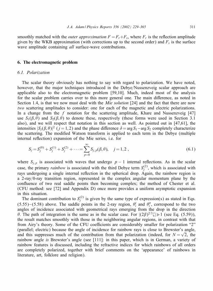
J.A. Adam /Physics Reports 356 (2002) 229–365 311
smoothly matched with the outer approximation F =Fr+Fs, where Fr is the reTection amplitudegiven by the WKB approximation (with corrections up to the second order) and Fs is the surfacewave amplitude containing all surface-wave contributions.
6. The electromagnetic problem
6.1. Polarization
The scalar theory obviously has nothing to say with regard to polarization. We have noted,however, that the major techniques introduced in the Debye=Nussenzveig scalar approach areapplicable also to the electromagnetic problem [59,10]. Much, indeed most of the analysisfor the scalar problem carries over to this more general one. The main di9erence, as noted inSection 1.4, is that we now must deal with the Mie solution [24] and the fact that there are nowtwo scattering amplitudes to consider: one for each of the magnetic and electric polarizations.In a change from the f notation for the scattering amplitude, Khare and Nussenzveig [47]use S1(; �) and S2(; �) to denote these, respectively (these forms were used in Section 3.1also), and we will respect that notation in this section as well. As pointed out in [47,61], theintensities |Sj(; �)|2 (j=1; 2) and the phase di9erence �=arg S1−arg S2 completely characterizethe scattering. The modiAed Watson transform is applied to each term in the Debye (multipleinternal reTection) expansion of the Mie series, i.e. for
Sj = S(0)j + S(1)
j + S(2)j + · · ·=
∞∑p=0
Sj;p(; �); j=1; 2 ; (6.1)
where Sj;p is associated with waves that undergo p − 1 internal reTections. As in the scalarcase, the primary rainbow is associated with the third Debye term S(2)
j , which is associated withrays undergoing a single internal reTection in the spherical drop. Again, the rainbow region isa 2-ray=0-ray transition region, represented in the complex angular momentum plane by theconTuence of two real saddle points then becoming complex; the method of Chester et al.(CFU method: see [72] and Appendix D) once more provides a uniform asymptotic expansionin this situation.
The dominant contribution to S(2)j is given by the same type of expression(s) as stated in Eqs.
(5.55)–(5.58) above. The saddle points in the 2-ray region, �′i and �′′i , correspond to the twoangles of incidence associated with geometrical rays emerging from the drop in the direction�. The path of integration is the same as in the scalar case. For |(2)2=3>|�1 (see Eq. (5.59)),the result matches smoothly with those in the neighboring angular regions, in contrast with thatfrom Airy’s theory. Some of the CFU coeYcients are considerably smaller for polarization “2”(parallel; electric) because the angle of incidence for rainbow rays is close to Brewster’s angle,and this suppresses much of the contribution from that polarization (indeed, for N =
√2, the
rainbow angle is Brewster’s angle (see [111]: in this paper, which is in German, a variety ofrainbow features is discussed, including the refractive indices for which rainbows of all ordersare completely polarized, together with brief comments on the ‘appearance’ of rainbows inliterature, art, folklore and religion).

312 J.A. Adam /Physics Reports 356 (2002) 229–365
There is of course a contribution to the rainbow region from the ray directly reTected atthe drop surface, represented by the Arst Debye term S(0)
j (; �), and this was included inthe numerical studies undertaken by Khare and Nussenzveig [59]. They compared the exactMie results (obtained, recall by summing over a number & of partial waves) for N =1:33;5066 1500, and 136◦6 �6 142◦ with both the Airy approximation and the results fromsystem (5.55)–(5.58). The main correction to the Airy theory is provided by the Ai′(−x) term(where x=− (2)2=3>) in Eq. (5.59). For polarization 1, within the main rainbow peak |x|. 1,the corrections to the Airy theory are small, but for the supernumerary arcs (x�1; secondarypeaks) they become signiAcant. For polarization 2 there are large corrections to the Airy the-ory, because the Ai′(−x) term is dominant throughout the complete range of interest. Becausethere is a change in sign of the amplitude reTection coeYcient at Brewster’s angle, one suchcorrection is that the secondary-peak maxima and minima should be interchanged for the twopolarizations (see also [7]). The results are compared in several Agures in [59]; in particularfor =500 oscillations with period ≈ (300=)◦ are superimposed on the main peak and part ofthe secondary (see Fig. 2 in [59]); this results from interference with the direct reTection term.Such interference remains appreciable up to =1500 (the upper value investigated; this is trueeven close to the rainbow angle �R), so the direct reTection term has been subtracted out intheir Fig. 3, which is reproduced here as Fig. 20. For the same value of the phase di9erence� is also plotted: the Airy theory fails here, even close to �R, whereas the exact results andasymptotic theory agree well throughout. Again, rapid oscillations arise from interference withdirect reTection. The authors point out that the oscillatory nature of the deviations between theasymptotic theory and the exact solution is consistent with interpreting them as “ripple”; this, aswe have noted above, is present in all directions (but dominant in the glory) is due to grazingincident rays which are in turn associated with Regge-pole-type contributions (surface waves)and higher-order Debye terms.
Concerning the glory, the same techniques apply, but for �=� the scattering amplitudes arerelated by
S1(; �)= SM () + SE()=− S2(; �) ; (6.2)
where the contributions from the magnetic multipoles (M) and the electric multipoles (E) areof the same order (this is called the cross-polarization e9ect [7,53,108]). Again, the object isto And which p values in the Debye expansion for each polarization yield signiAcant contri-butions at a given value of �; and thence to represent these by suitable asymptotic expansionsvia the modiAed Watson transform. There are in general four sets of contributions from (i)geometrical-optic rays (real isolated saddle-points in the �-plane); (ii) surface waves (complexRegge poles); (iii) rainbow terms (conTuent saddle points) and (iv) Fock-type transition regioncontributions (interpolating smoothly between (i) and (ii)). As we have seen in the scalar case,the contributions from geometrical optics are too insigniAcant to account for the glory; andwhile van de Hulst conjectured that p=2 surface waves are the dominant feature in describingthe phenomenon, as we have already seen, higher-order Debye terms need to be incorporatedfor a complete description.
For p�1, the important contributions come from the edge domain |� − | . 1=3, wherethe internal reTectivity is close to one. However, there are also contributions from higher-order
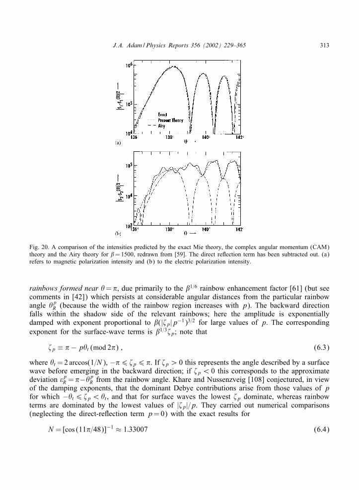
J.A. Adam /Physics Reports 356 (2002) 229–365 313
Fig. 20. A comparison of the intensities predicted by the exact Mie theory, the complex angular momentum (CAM)theory and the Airy theory for =1500, redrawn from [59]. The direct reTection term has been subtracted out. (a)refers to magnetic polarization intensity and (b) to the electric polarization intensity.
rainbows formed near �=�, due primarily to the 1=6 rainbow enhancement factor [61] (but seecomments in [42]) which persists at considerable angular distances from the particular rainbowangle �p
R (because the width of the rainbow region increases with p). The backward directionfalls within the shadow side of the relevant rainbows; here the amplitude is exponentiallydamped with exponent proportional to (|>p|p−1)3=2 for large values of p. The correspondingexponent for the surface-wave terms is 1=3>p; note that
>p ≡ �− p�t (mod 2�) ; (6.3)
where �t =2 arccos(1=N ), −�6 >p6�. If >p ¿ 0 this represents the angle described by a surfacewave before emerging in the backward direction; if >p ¡ 0 this corresponds to the approximatedeviation HpR =�−�p
R from the rainbow angle. Khare and Nussenzveig [108] conjectured, in viewof the damping exponents, that the dominant Debye contributions arise from those values of pfor which −�t6 >p ¡�t , and that for surface waves the lowest >p dominate, whereas rainbowterms are dominated by the lowest values of |>p|=p. They carried out numerical comparisons(neglecting the direct-reTection term p=0) with the exact results for
N =[cos (11�=48)]−1 ≈ 1:33007 (6.4)
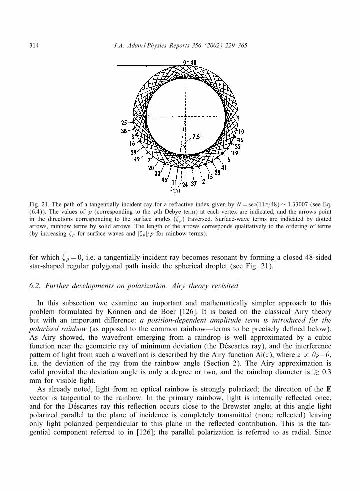
314 J.A. Adam /Physics Reports 356 (2002) 229–365
Fig. 21. The path of a tangentially incident ray for a refractive index given by N =sec(11�=48) � 1:33007 (see Eq.(6.4)). The values of p (corresponding to the pth Debye term) at each vertex are indicated, and the arrows pointin the directions corresponding to the surface angles (>p) traversed. Surface-wave terms are indicated by dottedarrows, rainbow terms by solid arrows. The length of the arrows corresponds qualitatively to the ordering of terms(by increasing >p for surface waves and |>p|=p for rainbow terms).
for which >p =0, i.e. a tangentially-incident ray becomes resonant by forming a closed 48-sidedstar-shaped regular polygonal path inside the spherical droplet (see Fig. 21).
6.2. Further developments on polarization: Airy theory revisited
In this subsection we examine an important and mathematically simpler approach to thisproblem formulated by KRonnen and de Boer [126]. It is based on the classical Airy theorybut with an important di9erence: a position-dependent amplitude term is introduced for thepolarized rainbow (as opposed to the common rainbow—terms to be precisely deAned below).As Airy showed, the wavefront emerging from a raindrop is well approximated by a cubicfunction near the geometric ray of minimum deviation (the D7escartes ray), and the interferencepattern of light from such a wavefront is described by the Airy function Ai(z), where z ˙ �R−�,i.e. the deviation of the ray from the rainbow angle (Section 2). The Airy approximation isvalid provided the deviation angle is only a degree or two, and the raindrop diameter is & 0:3mm for visible light.
As already noted, light from an optical rainbow is strongly polarized; the direction of the Evector is tangential to the rainbow. In the primary rainbow, light is internally reTected once,and for the D7escartes ray this reTection occurs close to the Brewster angle; at this angle lightpolarized parallel to the plane of incidence is completely transmitted (none reTected) leavingonly light polarized perpendicular to this plane in the reTected contribution. This is the tan-gential component referred to in [126]; the parallel polarization is referred to as radial. Since

J.A. Adam /Physics Reports 356 (2002) 229–365 315
the reTection angle for the D7escartes ray is several degrees away from the Brewster angle,some of the radial component is reTected to produce a correspondingly much weaker rainbow;it is this that we shall refer to as the polarized rainbow, the more intense common rainbowbeing tangentially polarized. It is interesting to note that the supernumerary bows (intensitymaxima) in the polarized rainbow are shifted to the locations of the minima in the commonrainbow; this was Arst observed in fog bows by Bricard [127]. From the geometrical opticsviewpoint, supernumerary bows are caused by interference between two rays with di9erentimpact parameters (and hence path lengths inside the drop) and the same scattering (devia-tion) angle. If the respective angles of incidence for these two rays, i1; i2 say, are such thati1 ¡IB ¡ i2, where IB is the Brewster angle, then these two rays have an additional phase dif-ference of 180◦ (see the very useful descriptions in KRonnen’s book [128]). This does not occurfor the corresponding rays in the common rainbow, so it is clear that constructive interferencein the latter is associated with destructive interference in the polarized rainbow, and this isconsistent with the numerical calculations of Khare and Nussenzveig [59]. Note also that thiscontrast will not be present in the secondary bow because of the two internal reTections in thedrop.
Near the Brewster angle the Fresnel coeYcient of reTection for parallel-polarized light variessubstantially (in relative terms), so that the wave amplitude cannot be considered constant alongthe wavefront, even near the rainbow angle. This contrasts with the case for perpendicularpolarization, for which the Fresnel coeYcient while varying, is never zero and so (in relativeterms again) the wave amplitude may be treated as constant to a Arst approximation. This is thebasis of the Airy approximation and while not completely satisfactory, provides a reasonablerepresentation of the common rainbow as we have seen.
The expression for the cubic wavefront has been noted earlier. A fuller account of its deriva-tion may be found in the book by Humphreys [18] to which we now refer. By consideringsmall deviations from the angles of incidence and refraction corresponding to the D7escartes ray,and with judicious use of Maclaurin’s theorem, Humphreys deduces that in a coordinate systemcentered on the point of inTection (see Eq. (2.3) above, where h=3c)
y=h
3a2 x3 ; (6.5)
where in terms of the order n of the rainbow and the refractive index N
h=(n2 + 2n)2
(n + 1)2(N 2 − 1)
{(n + 1)2 − N 2
N 2 − 1
}1=2
; (6.6)
a being as before the radius of the drop. For the primary rainbow (n=1) and N =1:33, h ≈ 4:9;for the secondary rainbow (n=2), h ≈ 28. Obviously h is not independent of N . Let IB; RBand IR be the Brewster angles of incidence, reTection and the angle of incidence for minimumdeviation respectively, and furthermore let 5= i − IR and �d = � − �R, where i and � refer togeneral angles of incidence and scattering, respectively. Then after some tedious but elementarymanipulations [18] we may write
x= a5 cos IR
316 J.A. Adam /Physics Reports 356 (2002) 229–365
and the integral superposition of the wave amplitude in the direction �d as
A=∫ ∞
−∞k(x) sin(!t − �) dx=A sin!t − B cos!t ; (6.7)
where k(x) is the wave amplitude per unit length along the wavefront, ! is the angular frequencyof the (monochromatic) light and � is the phase shift for a wave in direction �d from positionx with respect to a wave emanating from x=0 in the same direction. The expression for � is([18], see also Section 2)
�=2��
(hx3
3a2 cos �d − x sin �d
); (6.8)
where � is the wavelength of the light. We deAne the intensity I=A2 +B2 since (6.7) can bewritten in the form A=(A2 + B2)1=2 sin(!t − ,).
For the common rainbow, the Airy assumption is that k(x) is uniform throughout (and chosenhere as unity without loss of generality), and B=0 since � is an odd function of x, so for smallvalues of �d the standard Airy intensity is obtained as A2 where
A=∫ ∞
−∞cos
2��
(hx3
3a2 − x�d
)dx : (6.9)
The situation is more complicated for the polarized rainbow. For the primary rainbow A⊥ andA|| refer to the amplitudes of light with the E vector perpendicular and parallel to the plane ofincidence, respectively. Then by Fresnel’s equations (for unit amplitude incident light)
A⊥ =[1− sin2(r − i)
sin2(r + i)
] [sin(r − i)sin(r + i)
](6.10)
and
A|| =−[1− tan2(r − i)
tan2(r + i)
]2 [ tan(r − i)tan(r + i)
]: (6.11)
Note again that A|| changes sign if i passes through IB. If 6= i − IB; H= r − RB then usingSnell’s law it follows for small 6 and H that
H=cos IB
N cosRB6=
6N 2
from which
k(x)=A||A⊥
� 6 + Hcos3(IB − RB)
or
k(x) � (1 + N−2)6cos3(IB − RB)
≈ 1:776=1:77
a cos IR(x + x0) ; (6.12)
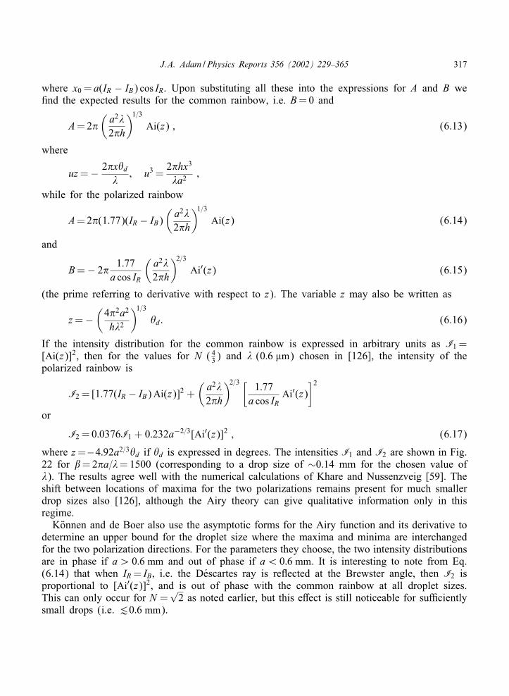
J.A. Adam /Physics Reports 356 (2002) 229–365 317
where x0 = a(IR − IB) cos IR. Upon substituting all these into the expressions for A and B weAnd the expected results for the common rainbow, i.e. B=0 and
A=2�(
a2�2�h
)1=3Ai(z) ; (6.13)
where
uz=− 2�x�d
�; u3 =
2�hx3
�a2 ;
while for the polarized rainbow
A=2�(1:77)(IR − IB)(
a2�2�h
)1=3Ai(z) (6.14)
and
B=− 2�1:77
a cos IR
(a2�2�h
)2=3Ai′(z) (6.15)
(the prime referring to derivative with respect to z). The variable z may also be written as
z=−(
4�2a2
h�2
)1=3�d: (6.16)
If the intensity distribution for the common rainbow is expressed in arbitrary units as I1 =[Ai(z)]2, then for the values for N (4
3) and � (0:6 �m) chosen in [126], the intensity of thepolarized rainbow is
I2 = [1:77(IR − IB)Ai(z)]2 +(
a2�2�h
)2=3 [ 1:77a cos IR
Ai′(z)]2
or
I2 =0:0376I1 + 0:232a−2=3[Ai′(z)]2 ; (6.17)
where z=−4:92a2=3�d if �d is expressed in degrees. The intensities I1 and I2 are shown in Fig.22 for =2�a=�=1500 (corresponding to a drop size of ∼0:14 mm for the chosen value of�). The results agree well with the numerical calculations of Khare and Nussenzveig [59]. Theshift between locations of maxima for the two polarizations remains present for much smallerdrop sizes also [126], although the Airy theory can give qualitative information only in thisregime.
KRonnen and de Boer also use the asymptotic forms for the Airy function and its derivative todetermine an upper bound for the droplet size where the maxima and minima are interchangedfor the two polarization directions. For the parameters they choose, the two intensity distributionsare in phase if a¿ 0:6 mm and out of phase if a¡ 0:6 mm. It is interesting to note from Eq.(6.14) that when IR = IB, i.e. the D7escartes ray is reTected at the Brewster angle, then I2 isproportional to [Ai′(z)]2, and is out of phase with the common rainbow at all droplet sizes.This can only occur for N =
√2 as noted earlier, but this e9ect is still noticeable for suYciently
small drops (i.e. .0:6 mm).
318 J.A. Adam /Physics Reports 356 (2002) 229–365
Fig. 22. The light intensity distribution as a function of � − �R for both rainbow polarizations: (a) the “common”rainbow and (b) the polarized rainbow. This corresponds, respectively, to the E vector (a) tangential and (b) radialwith respect to the rainbow arc. The scattering angle is � and the rainbow angle is �R. The calculations are forsize parameter =1500 which corresponds to a droplet radius of approximately 0:14 mm in visible light. Note thedi9erences in the positions of the supernumerary bows in the two Agures. (Redrawn from [126].)
Returning to the choice k(x)=1, made earlier for the classical Airy approximation to thecommon rainbow, it is of course possible to extend that theory by including the variation in thereTection coeYcient for A⊥ also. This in fact contributes only a small correction to the Airytheory: the term in Ai′(z) is never dominant. However, the minima in this case are never zero,which is also in agreement with the results reported in [59]. Similar calculations were performedfor the secondary rainbow; deviations from the Airy theory are less pronounced, even for thepolarized rainbow, where the expression for I2 contains terms in Ai2(z) and Ai′′(z) only; sincethese terms are proportional (see e.g. [129]) the intensity oscillations remain in phase with thoseof the common secondary rainbow.
Finally, the degree of polarization can be easily determined using this formalism. At therainbow angle �d =0; so from Eq. (6.17) it follows that
I2
I1=R(a)=0:036 + 0:00465a−2=3 ; (6.18)
which for large a compares well with the geometrical optics result [111] of R=0:039, especiallyas a→∞. However, since R as written here increases monotonically as a→ 0, for small values of
J.A. Adam /Physics Reports 356 (2002) 229–365 319
a it is more appropriate to consider R as the ratio of the maxima of the intensity distributions forz �=0. By taking values of z equal to −3:25 (common rainbow) and −4:08 (polarized rainbow)as representative maxima (the Arst supernumerary bows) KRonnen and de Boer obtain
R(a)=0:0087a−2=3[Ai′(−4:08)Ai(−3:25)
]2=0:032a−2=3 ; (6.19)
R(0:14)=0:12 (a is in mm) which is to be compared with the prediction of 0:054 from theabove asymptotic-type geometrical optics result. This implies that the polarized rainbow is morereadily observable for small droplets (e.g. as in fogbows) than is predicted by geometrical optics.
6.3. Comparison of theories
There have been several comparisons between some or all of the following: geometricaloptics, Mie theory and the Airy approximation. Ungut et al. [43] studied the scattered light fromtransparent spherical particles with a range of diameters from 1 to 100 �m, and in the forwardscattering angle range 0◦–20◦; and compared the results of Mie theory and geometrical optics.For the parameter ranges considered they concluded that the latter is a reasonable approximationto the former, especially if the particles are assumed to deviate from perfect sphericity in anycross-sectional area by a change in the diameter �d � �. More recently, Wang and van deHulst [42] have given a detailed computational account of an eYcient and accurate method ofevaluating the Mie coeYcients for . 50 000, corresponding to drop diameters up to ∼6 mmfor visible light. They also compare their Mie theory calculations with the Airy approximation(generalized to an arbitrary number of internal reTections; this number is denoted by p −1; p¿ 1, consistent with the notation in [6] and Section 5 above). SpeciAcally they And thatfor drop diameters ∼ 1 mm there is agreement in all details, including the polarization and theposition and intensity of the supernumerary maxima; this agreement is still fairly good down toa diameter of ∼ 0:1 mm. It transpires that the higher the value of the refractive index, the closeris the agreement between the two theories for the primary rainbow (p=2) for drop diametersas small as 0:02 mm. They also investigate Alexander’s dark band and conclude that in additionto the presence of externally reTected light (p=1) there is a signiAcant contribution from thep=6 and 7 rainbows. The positions of these are very sensitive to the wavelength of the light.
We note some other points from this paper, the Arst being of historical interest. The authorspoint out that since 1957 (when Van de Hulst’s book [7] Arst appeared) the large gap thatexisted between small -values, for which Mie theory was computationally feasible, and large-values, for which the Airy theory is valid, is much closer to being closed today. This gapwas 30 . . 2000, and since that time (as detailed earlier) the complex angular momentumtheory ([10] and many references therein) and the development of highly eYcient computationalschemes have helped to close the gap (from the upper and lower ends, respectively). Now,reliable Mie computations are feasible for up to at least 50 000. Details of these can befound in [42].
We have alluded earlier to the curvature term h=3a2 for the cubic wavefront approximation ofAiry (see Eqs. (6.5) and (6.6)), where h is expressed in terms of the order of the rainbow andthe refractive index. Note that the curvature of the wavefront is greater for higher values of p(and hence n) and smaller values of a (or, for light of a given wavelength, for smaller values

320 J.A. Adam /Physics Reports 356 (2002) 229–365
of ), so that the angular spacing between two successive supernumerary peaks increases withincreasing p (or n) and=or with decreasing a. In both [7] and its relatively recent extension [42]an expression is given for the rainbow peak intensity: in particular there is a size dependenceof ∼ x7=3 which is consistent with an amplitude dependence of ∼x7=6 in Eq. (2.4) of [61], sothere is no discrepancy in this regard between the two approaches, i.e. between the Airy theoryand the complex angular momentum theory. For a drop with diameter 3:2 mm, the authors alsofound excellent agreement between the Mie and the Airy theories (such a large drop would not,of course retain its spherical shape in the atmosphere). The primary rainbow was found to be≈ 7:7 (red light) to ≈ 8:4 (violet light) times more intense than the secondary rainbow, and allthe Airy maxima up to about the tenth supernumerary bow were at the predicted angles andhad the correct intensities. Also the angular separation of the rainbows was found to decreaseas the light shifted from violet to red: the shift in the secondary (p=3) being twice that in theprimary (p=2) rainbow.
For a drop diameter of 0:1 mm there is still (surprisingly, as the authors point out) goodagreement between the Mie and Airy intensities for the Arst maxima in cases p=2 and 3.Amongst other features, the dark band is still seen in the violet but diminishes in the red, andthe Airy theory predicts somewhat larger shifts in the higher supernumerary bow positions forp=2 and 3. Tests for even smaller sizes (and various refractive indices) indicate that the Airytheory predicts well the features of the Arst peak of the primary rainbow. In the dark band,where the intensity may drop to below 0:5% of that in the primary peak, the intensity is wellexplained as contributions from the p=0 (external reTection) and the p=6 and 7 rainbows.The overall conclusion drawn by Wang and van de Hulst is that the Airy theory providessimple and reliable information over a wide range of sizes, and furthermore this may be usefulin determining properties of particles in laboratory, meteorological or astronomical experiments.
Related to these results is a set of observations made earlier by Sassen [1] in connectionwith angular scattering and rainbow formation in pendant drops. These are laboratory-producednear-spherical drops with certain similarities to the shape of distorted raindrops. The latterbecome increasingly oblate and unstable with increasing size, and tend to orient themselvesuniformly in space as they fall. Measurable raindrop distortions have been noted for drops assmall as 0:3 mm in diameter [130] and are signiAcant for diameters &1 mm. As might thereforebe expected, rainbow features often vary with the position of the generator of the rainbow “cone”as the observer views di9erent parts of the rainbow. This is because of the change in geometriccross-section of the drop as the angle of observation changes (for more on this see Section 6.4).Such variations have been observed [131]. Obviously in any given situation it is expected thatthere will be a distribution in raindrop size. It is frequently the case that rainfall from convectiveshowers (conditions under which rainbows are frequently observed) contain “supermillimeter”drops, so information on near-spherical drops may well help to explain occasional anomalousfeatures (i.e. unlikely to occur for purely spherical drops) such as reports of tertiary rainbows[14,132–134] at 42◦ (while standard theory predicts their existence, they are considered toofaint and too close to the sun’s position to be observable, although these reports might refer toreTected or reTected-light rainbows [4]).
The pendant drops discussed in [1] are more akin in shape to the familiar “teardrop” shapeso beloved of cartoonists. Nevertheless, they combine spherical and non-spherical scatteringmechanisms that are considered relevant to those for aspherical raindrops for the following
J.A. Adam /Physics Reports 356 (2002) 229–365 321
two reasons: (i) they retain a circular cross section in a horizontal plane and (ii) display areduction in surface curvature (compared to a spherical drop) along the vertical sides of thedrop. These are exactly the same features displayed by the “hamburger-bun” shapes of largerraindrops (see further references in [1] for details of numerical and theoretical simulations ofrealistic raindrop shapes). Angular scattering experiments revealed that such near-spherical dropsgenerate exceptionally well-deAned primary, secondary and associated supernumerary bows, butunexpectedly strong higher-order bows as well, perhaps because of the reduced curvature in thecentral elongated regions, thus providing relatively more surface area within the drop availablefor generating rainbow rays. As with the later work of Wang and van de Hulst [42], it wasfound that the precise angular positions of at least the Arst 10 intensity maxima for the primaryand secondary rainbows were predicted by the Airy theory. Interestingly, it is claimed that thetheory fails to account for the position of the sixth-order rainbow (p=7), but in [42] it wasfound that this rainbow, along with that for p=6 is found just inside Alexander’s dark band.
Dave [135] presented results of Mie computations for large non-absorbing spheres and com-pared them with those corresponding to geometrical and physical optics (i.e. including di9rac-tion e9ects). This was done for monochromatic radiation of wavelength �=0:4 �m and waterspheres of radii a=6:25; 12:5; 25 and 50 �m, corresponding to size parameters, respectively,of =31:25�; 62:5�; 125� and 250�, well below the region of applicability (and prior to theemergence of the complex angular momentum theory) of the classical ray and Airy theories [7].Dave considered three regimes using geometrical optics: forward scattering, the rainbow regionand the glory region. An approximate value for the scattered intensity in the Arst regime canbe found by replacing the sphere by a circular disk of radius a [7]. This unpolarized di9ractedradiation has intensity
If =4[J1( sin �) sin �
]2;
relative to the incident radiation intensity. The maximum intensity of 4=4 occurs of course at�=0◦; successive minima and maxima occur as � increases away from zero. If the amplitudesof the reTected and refracted are comparable with that of this di9racted component, there can bea signiAcant increase in intensity and interference between these components. (This is sometimesreferred to as “anomalous di9raction” mentioned earlier; further details may be found in [7].)Similar interference phenomena may of course occur in the rainbow region on either side of theD7escartes ray of minimum deviation, if two such rays emerge in parallel directions—leadingat this level of description to an explanation of the supernumerary bows. Apart from van deHulst’s suggestion of surface wave involvement as responsible (in part) for the glory, therewas at that time no satisfactory detailed account of this phenomenon (the work by Nussenzveigwas published shortly after [135] appeared). This paper [135] provides many Agures and relatedresults; it was concluded on the basis of the four size parameters studied that ray optics andMie theory agree well only if ∼ 800 (and presumably & 800, though Dave’s largest valuewas =785:4). He concluded that a satisfactory explanation of the glory should await a moresubstantial understanding of surface waves and the interaction between radiation Aelds (true),and noted also the lack of a simple explanation for (i) anomalous di9raction in the forwarddirection (for �¿ 2◦) and (ii) the appearance of several distinct maxima outside the regions ofprimary and secondary rainbows.
322 J.A. Adam /Physics Reports 356 (2002) 229–365
The four approaches to the theory of the rainbow discussed so far are, in historical order:geometrical optics, Airy’s approximation, Mie theory and complex angular momentum theory.Crudely, the Arst of these is independent of size of the drop, but only valid for large sizeparameters, e.g. & 5000. Airy’s approximation is valid for & 5000 and for |�−�R|. 0:5◦;the Mie solution is exact but requires the summation of a number of partial waves greater than (this is no longer the problem it used to be for & 100 as noted above in connection with[42]). The complex angular momentum theory provides a very good substitute for Mie theoryif & 50 (in fact it is still very accurate for & 1 [10]) but is mathematically very technical.It was with these restrictions in mind that Mobbs [136] developed another theory, based onHuygens’ principle (as is Airy’s theory) in which he states that the physics is straightforward andonly simple computation is required for a substantial range of drop sizes. A virtual wavefrontleaving the drop after one internal reTection is examined, as in Airy’s theory, and a set ofequations is developed which completely deAnes this wavefront. Mobbs also deAnes, in a similarmanner, a virtual wavefront for the externally reTected ray. The distributions of amplitude (forboth polarizations) depend on the drop geometry, the wavefront and the Fresnel amplitudecoeYcients. Sixteen Fresnel zones were constructed across the wavefront, each of which has anamplitude (uniform across the zone) characteristic of the total light Tux passing through thatzone. Thus the wavefronts consisted of 16 annular rings around the (obvious) central axis (z)of the drop; the boundaries corresponding approximately to equally spaced values of the angleof incidence. The basic mathematical features of this approached will be brieTy summarizedhere (and in the opinion of this author, with regard to Mobbs’ earlier comment about the CAMtheory, his calculations are not entirely without mathematical complexity either!).
Suppose that the nth zone, 16 n6 16, lies in the angle of incidence interval [in; in+1]. Thearea orthogonally presented to the incident light between these angles is readily shown to be
an =�a2
2(cos 2in − cos 2in+1) (6.20)
and the area of the zone is, in a cylindrical polar coordinate system,
An =2�∫ in+1
inR
[1 +
(dzdR
)2]1=2dRdi
di : (6.21)
DeAne
Gp;n =(
anAp;n
)1=2;
where the subscript p refers to externally reTected light (p=0) and internally reTected lightfor the primary rainbow (p=2). The rainbow rays undergo two refractions (transmissions) anda single reTection. So using the Fresnel amplitude coeYcients the amplitude corresponding tothe nth zone is given by
A(1)2; n =G2; n
sin(2i) sin(2r) sin(i − r)sin3(r + i)
(6.22)

J.A. Adam /Physics Reports 356 (2002) 229–365 323
for polarization 1 (magnetic) and
A(2)2; n =G2; n
4 sin(2i) sin(2r) tan(i − r)[sin(2i) + sin(2r)]2 tan(r + i)
(6.23)
for polarization 2 (electric). The corresponding amplitudes for externally reTected light are
A(1)0; n =−G0; n
sin(i − r)sin(i + r)
(6.24)
and
A(2)0; n =G0; n
tan(i − r)tan(i + r)
: (6.25)
Mobbs then applies Fresnel’s formulation of Huygen’s principle by examining the path di9erencebetween rays that meet the wavefronts such that 1=�−�R. The disturbance from an element ofarea dS of the wavefront near a point P, a large distance s from the drop can then be expressedin terms of the A coeYcients above, some complex exponential factors in time and space, andan obliquity factor, details of which may be found in [136]. By suitable formal integrations,using results of the type [105]∫ �
0cos(n�− x sin �) d�=�Jn(x); n=0; 1; 2; : : : (6.26)
and after considerable reduction, the amplitude coeYcients S( j)p (�; ) can be written in terms of
the rather formidable expression
S( j)p (�; )=
16∑n=1
�A( j)p;n(�
−1 tan 1)e−iklp sin 1[RpJ1(kRp sin 1)eikzp cos 1]Rp; in+1Rp; in
−16∑n=1
�A( j)p;n(k�
−1)e−klp sin 1
( ∫ in+1
inRp
[1 +
(dzpdRp
)2]1=2
+ sec �
×eikzp cos 1J0(kRp sin 1)dRp
didi
); (6.27)
where the path di9erence calculated is between light from the point (lp; 0; 0) and the pointP(Rp; ,; zp). The addition of the contributions from the internally and externally reTected lightis carefully considered in terms of the phase di9erence between the two; then the totalamplitude coeYcients S(j)(�; ) are
S(j)(�; )=Re(S( j)2 ) + Re(S( j)
0 ) cos − Im(S( j)0 ) sin
+i[Im(S( j)2 ) + Re(S( j)
0 ) sin + Im(S( j)0 ) cos ] : (6.28)
Concerning the validity of this approach, Mobbs makes an interesting point: its validity isbased on the assumption that the wavefronts can be determined by constructing rays (orthogonal
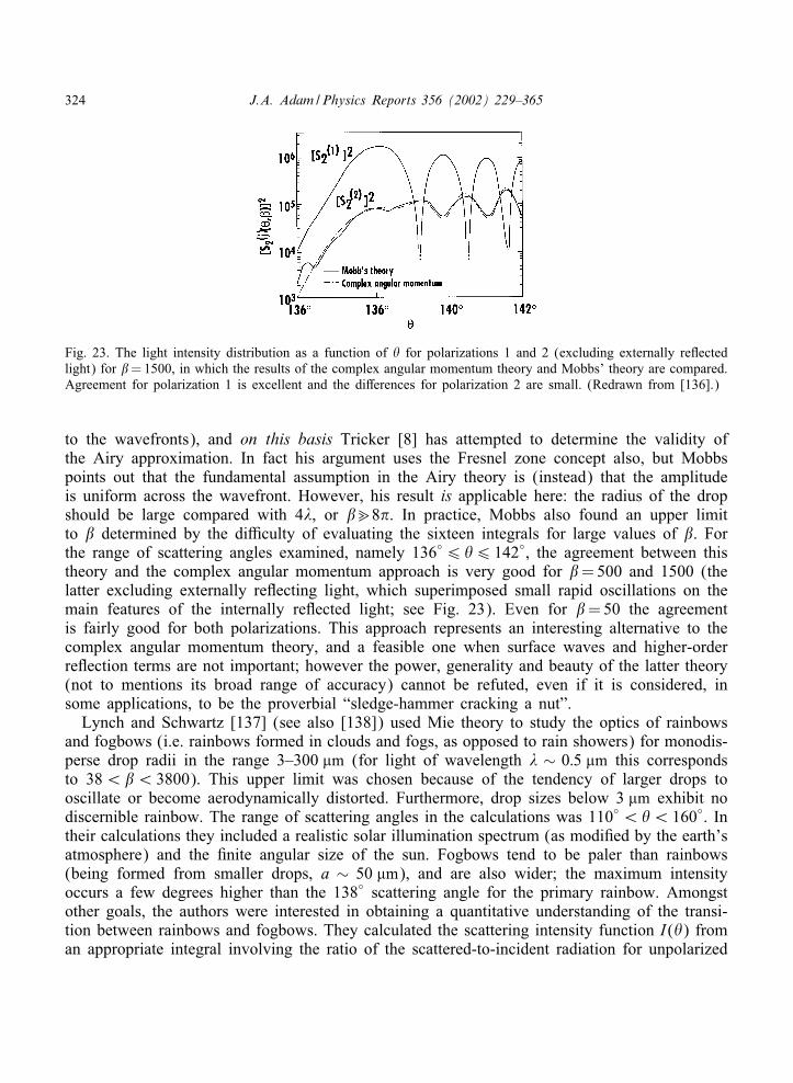
324 J.A. Adam /Physics Reports 356 (2002) 229–365
Fig. 23. The light intensity distribution as a function of � for polarizations 1 and 2 (excluding externally reTectedlight) for =1500, in which the results of the complex angular momentum theory and Mobbs’ theory are compared.Agreement for polarization 1 is excellent and the di9erences for polarization 2 are small. (Redrawn from [136].)
to the wavefronts), and on this basis Tricker [8] has attempted to determine the validity ofthe Airy approximation. In fact his argument uses the Fresnel zone concept also, but Mobbspoints out that the fundamental assumption in the Airy theory is (instead) that the amplitudeis uniform across the wavefront. However, his result is applicable here: the radius of the dropshould be large compared with 4�, or �8�. In practice, Mobbs also found an upper limitto determined by the diYculty of evaluating the sixteen integrals for large values of . Forthe range of scattering angles examined, namely 136◦6 �6 142◦, the agreement between thistheory and the complex angular momentum approach is very good for =500 and 1500 (thelatter excluding externally reTecting light, which superimposed small rapid oscillations on themain features of the internally reTected light; see Fig. 23). Even for =50 the agreementis fairly good for both polarizations. This approach represents an interesting alternative to thecomplex angular momentum theory, and a feasible one when surface waves and higher-orderreTection terms are not important; however the power, generality and beauty of the latter theory(not to mentions its broad range of accuracy) cannot be refuted, even if it is considered, insome applications, to be the proverbial “sledge-hammer cracking a nut”.
Lynch and Schwartz [137] (see also [138]) used Mie theory to study the optics of rainbowsand fogbows (i.e. rainbows formed in clouds and fogs, as opposed to rain showers) for monodis-perse drop radii in the range 3–300 �m (for light of wavelength � ∼ 0:5 �m this correspondsto 38¡¡ 3800). This upper limit was chosen because of the tendency of larger drops tooscillate or become aerodynamically distorted. Furthermore, drop sizes below 3 �m exhibit nodiscernible rainbow. The range of scattering angles in the calculations was 110◦ ¡�¡ 160◦. Intheir calculations they included a realistic solar illumination spectrum (as modiAed by the earth’satmosphere) and the Anite angular size of the sun. Fogbows tend to be paler than rainbows(being formed from smaller drops, a ∼ 50 �m), and are also wider; the maximum intensityoccurs a few degrees higher than the 138◦ scattering angle for the primary rainbow. Amongstother goals, the authors were interested in obtaining a quantitative understanding of the transi-tion between rainbows and fogbows. They calculated the scattering intensity function I(�) froman appropriate integral involving the ratio of the scattered-to-incident radiation for unpolarized
J.A. Adam /Physics Reports 356 (2002) 229–365 325
light; this latter quantity is the scattering matrix element S11(a; �; �) in their notation. (To usetheir results to model a rainbow formed in a rain shower would require I(�) to be weightedwith the drop distribution n(a) and an additional cross-section factor.) In particular, for theranges considered the authors found that:
(i) the rainbow attains a minimum angular width for a=100 �m. Indeed, as a decreasesthe widths of both primary and secondary bows increase, their contrasts (as deAned in [137])decrease and their scattering angles of maximum brightness move away from Alexander’s darkband.
(ii) the supernumerary bows for the primary rainbow attain maximum visibility for a=50 �m;they grow wider and further apart as a decreases. For values of a above about 56 �m theirseparation is less than the sun’s angular diameter of 0:5◦ and their amplitudes are greatlyreduced as a result of the concomitant smoothing e9ect; below about 36 �m the wider bowslose contrast. There are other factors inTuencing this of course, such as drop size, shape anddistribution [139,140].
(iii) Alexander’s dark band maintains a constant angular width of about 9:5◦, apparentlybecause the primary and secondary bows, while widening grow away from the dark band withdecreasing drop size; its angular width, however, is a function of drop size;
(iv) the maximum linear polarization of both types of bow is also a function of drop size,reaching a maximum of 90% for the primary bow and 50% for the secondary bow when20 �m¡a¡ 100 �m, and
(v) the secondary fogbow is observable only when a¿ 10 �m. The authors further suggestthat a fogbow be deAned as any rainbow formed in drops for which a¡ 35 �m.
In 1983, Fraser published a paper with the intriguing title “Why can the supernumerarybows be seen in a rainshower?” [141]. In order to see why there should be such a questionin the Arst place a little background will be useful. The supernumerary bows are essentially aninterference phenomenon, as Young pointed out in the Bakerian Lecture of 1802 [142]. TheAiry approximation predicts, as we have seen, that the spacing between adjacent bows, and thewidth of the primary bow should increase with decreasing drop radius. Since in reality however,normal rainshowers have a spectrum of drop radii (spanning more than an order of magnitude[143]) it would seem that no consistent pattern of supernumeraries should be seen, contrary towhat is frequently observed. These bows form near the top of the bow, and so any explanationof their existence should incorporate the fact that the light in this portion passes through thevertical cross section of often-distorted drops.
While the standard ray approach (supplemented by the wave concept of interference) isa perfectly reasonable way to explain the existence of supernumerary bows for two sets ofrays emerging in the same direction from monodisperse drops, Fraser points out that “a morecompelling visualization is obtained if the rays are replaced by waves”, and this is certainly thecase (see Fig. 4). The ray picture cannot of course account for di9erent drop sizes, whereasthe wave picture does, and indicates that large drops yield tightly spaced supernumeraries withnarrow maxima, while small drops yield broader maxima with wider spacing. Fraser uses theAiry approximation in his calculations, pointing out that it does adequately identify the positionsof the maxima for drop radii in excess of 0:05 mm (50 �m), which is certainly outside thefogbow range according to [137]. The angle of minimum deviation is a9ected by drop distortion:MRobius showed that the deviation angle of the D7escartes ray would in fact be increased [144].
326 J.A. Adam /Physics Reports 356 (2002) 229–365
Fraser used ellipsoidal drops in his calculations, noting that for the smaller drop sizes of interestto him, this is an excellent approximation. It appears that the minimum angle of deviation isalso weakly dependent on solar elevation (presumably because of the di9erent-sized drops thatcontribute to the light distribution at the top of the rainbow), but only one such elevation (0◦)was used since this e9ect is negligible here. Since smaller drops yield larger angles for theD7escartes ray, it is apparent that there is an intermediate drop size that will yield a minimumdeviation angle D, i.e. in formal terms
D(a)=mina{min
iD(i)}
and it these drops which cause the supernumeraries that are observed. This drop size turnsout to be in the range 0.1–0:2 mm for the primary bow and in the range 0.2–0:3 mm for theArst two supernumeraries. No other drops make a signiAcant contribution. On the basis of hisresults Fraser predicts that if supernumerary bows are seen in a rain shower, their separationwill be ∼ 0:75◦, independent of the particular size distribution of the raindrops, and found fromphotographs typical separations of ∼ 0:70◦:
In addition, Fraser [145] has pointed out that the explanation by Voltz [150] for the absenceof supernumerary bows near the base of the primary rainbow (when the sun is low in thesky) also applies to the intensiAcation of the red light contribution in the same location. (Healso states that the rainbow is a Ane example of a phenomenon in which theory tends to colorobservations.) Near the top of a rainbow the red color is much less intense that towards thebase, i.e. the more nearly vertical portions of the bow. It is only in these regions that theincident light, which is deviated in a more nearly horizontal plane, encounters a circular crosssection in a Tattened drop. Large drops will still contribute to the rainbow, whereas such dropsin the vertical plane displace the rainbow angle inward toward the antisolar point because oftheir distorted cross section in that plane (this was in fact Arst demonstrated by MRobius [144]:elliptical drops lower the top of the bow. Voltz estimates that drops smaller in radius than 0.25–0:5 mm are suYciently spherical to contribute to all portions of the rainbow; larger than this theywill contribute only to the vertical portions, which in turn explains why the rainbow is brightestthere—the larger drops substantially increase the intensity—and why the supernumeraries areabsent—the intensity maxima overlap. The complete spectrum of “colors of the rainbow” mayonly occur near the foot of the bow (along with the pot of gold, etc.).
6.4. Non-spherical (non-pendant) drops
Subsequently, and perhaps inspired by the work of Fraser, KRonnen discussed the same type ofphenomena in more mathematical detail, but speciAcally for the secondary rainbow [147]. They(i.e. supernumeraries for the secondary bow) are seen only on extremely rare occasions [148].KRonnen points out that the D7escartes ray for the secondary rainbow shows very little dependenceon the drop oblateness (for visible light) due to the fact that oblateness-induced changes in thetwo refractions and two interior reTections essentially cancel out, and so in view of Fraser’sexplanation for supernumeraries associated with the primary bow, they are unlikely to be seenfor the secondary bow (for most solar elevations there is now no stationary point for D(a)).However, for solar elevations exceeding about 35◦ the Tattening of the drops can result in a
J.A. Adam /Physics Reports 356 (2002) 229–365 327
minimum for D(a), and this may be suYcient to cause the Arst supernumerary—particularlyfor red light—to become visible (see [147] for a detailed explanation). KRonnen approximates afalling drop by an oblate spheroid, with its two semi-major axes of length a horizontal and itssemi-minor axis of length b vertical. The equivalent (i.e. same volume) spherical drop radiusis r=(a2b)1=3 and for r¡ 1:2 mm this is a reasonable approximation (and an excellent one ifr¡ 0:5 mm). Following MRobius [144] the drop ellipticity is deAned as
G=a− ba + b
: (6.29)
For drops falling at terminal velocity (assumed here) Green [149] derived an approximaterelationship between the ratio b=a and r. It is given by
ba−1 = [(4=17)(17B=4 + 1)1=2 + 13=17]−3=2 ; (6.30)
where B=G′r2g′=/ is called the Bond number; G′; g′ and / are respectively the drop density,e9ective gravity (g′ =(G − Gair)G−1g) and surface tension coeYcient. By substituting this intothe expression above for G and expanding in a Maclaurin series about r2 =0, KRonnen obtainsthe further approximation G � 0:05r2 if r is expressed in millimeters. He states that this simpleresult is useful for r¡ 1:5 mm. According to [144] the deviation between the rainbow anglesfor spheroidal and spherical drops is
]�R ≡ �R(spheroid)− �R(sphere) ;
i.e.
]�R =180◦
�16G sin cos3 cos(2h− 42◦) ; (6.31)
where here is the angle of refraction of the D7escartes ray for spheres, h is the (angular) solarelevation and 42◦ (=180◦ − �R(sphere)) is the angular distance from the bow to the antisolarpoint. (KRonnen also notes a sign error, and signiAcant consequences therefrom, present in [152]).For angles of observation other than for the top of the bow, (i.e. a non-vertical scattering plane)the corrections to G and h are also provided in [147]. In the visible range the angle (� 40◦)varies by only about 1◦, so equation (6.31) is almost independent of wavelength. Furthermore,it is consistent with Fraser’s conclusions that ]�R is a strong function of drop radius r butonly a weak function of h (h¡ 42◦). Thus to a good approximation,
]�R =13◦r2 cos(2h− 42◦) ≡ Cr2; (6.32)
where 10◦6C6 13◦: The result corresponding to (6.31) for the secondary rainbow is
]�R =− 180◦
�64G sin cos3 cos 2 cos(2h− 51◦) ; (6.33)
where the negative sign results from changing the scattering angle interval to [180◦; 360◦], whichenables the results for the primary and secondary bows to be presented in a more convenientand consistent manner. Note that in this case ]�R is zero when =45◦; it is a straightforward
328 J.A. Adam /Physics Reports 356 (2002) 229–365
matter to show from geometrical optics that
cos 2=5N 2 − 9
4N 2
and so this occurs when N =√
9=5 � 1:342, which for water corresponds to violet light. Thisof course means that now there is a strong dependence of ]�R on wavelength for light thiswavelength, which is readily formulated using di9erentials. It turns out to be necessary to includeterms up to G2 for the secondary rainbow, the result corresponding to (6.32) above being
]�R =C1r2 + C2r4; (6.34)
where the coeYcients C1 and C2 are deAned in [147]. The author further demonstrates that thestationary behavior for the secondary rainbow near its Arst supernumerary occurs if r � 0:7 mm;this in turn leads to a yet simpler form for (6.34), namely ]�R =C ′r2, where C ′ =C1 + 0:5C2:C ′ is a strong function of wavelength (via C1) and solar elevation (via C2).
For falling drops not exceeding about 1:8 mm in radius (G ≈ 0:1), the Airy theory can still beapplied if the rainbow angle for spheres is replaced by that for spheroids using the expression for]�R: For larger eccentricities this is not the case, because the Airy intensity distribution (whichmay be thought of as corresponding to a fold di;raction catastrophe) may be transformedinto a hyperbolic umbilic di;raction catastrophe in any given drop of large enough G. Thisis because two additional rays with skew paths through the drop can also contribute to therainbow interference pattern [151]. (Di9raction catastrophes will be discussed in more detail inSection 7). This has been observed to occur for the primary rainbow when the scattering planeis approximately horizontal [147]. For reasons discussed in that paper, it is conjectured that nosuch transformation occurs for the secondary rainbow (though it may occur for other refractiveindices). Furthermore this e9ect can be neglected if there is a broad distribution of drop sizes,because for the Marshall-Palmer distribution [152] (for example) less than 1% of the dropsexceed 1:5 mm in radius, so the e9ect is swamped by that from the smaller drops.
Returning to the regime for which the analytic form from the Airy theory is still appropriate,the following expression arises for the intensity distribution near the secondary rainbow angle�R (� 231◦)
I(r; �)˙ r7=3 Ai2[f(r; �; �)] ; (6.35)
where f(r; �; �) (not to be confused with the scattering amplitude) is deAned as:
f(r; �; �)=− 3:1(
500r�
)2=3[�− �R(sphere)− Cr2] : (6.36)
The same functional form applies to the primary rainbow also with some di9erences in theargument of the Airy function. The above argument is stationary at r= rs where
4Cr2s = �− �R(sphere) :
If C ¿ 0, the stationary behavior of f is in the oscillatory region of the Airy function, whichmeans that the integral of Eq. (6.35) over a broad drop-size distribution also has an oscillatory
J.A. Adam /Physics Reports 356 (2002) 229–365 329
component, and the spacing between consecutive maxima in the intensity distribution can beinferred from this. The angular spacing �1;2(�; h) between the Arst and second supernumerarybows is given in [147] by the expression
�1;2(�; h)=0:71◦C1=4(�; h)(
�640
)1=2: (6.37)
For the primary bow with C =13◦; �1;2 =0:88◦ at �=640 nm, consistent with the results ofFraser [141]; for the secondary bow with C =1◦ at the same wavelength, �1;2 =0:71◦:
In order to simulate the intensity distribution of a typical secondary bow produced by a raincloud, KRonnen assumed the drop-size distribution to be of the Marshall-Palmer type [152]
dndr˙ exp(−6r) ;
where n is the number of particles of radius r (in mm). This relation was then multiplied by(6.35) and integrated over both r and the solar disk. Amongst KRonnen’s conclusions were thefollowing: (i) the intensity of the main peak of the secondary bow is a factor of 4 greater at thetop than at the base; (ii) at low solar elevations, no supernumeraries (for the secondary bow)should ever be observed; and (iii) at higher solar elevations the Arst supernumerary should beobservable, especially at the red end of the visible spectrum if a Alter is used. The primaryreason for the diYculty of observing the supernumerary bows is that the secondary rainbowangle is much less sensitive to the Tattening of rain drops than is the corresponding angle forthe primary bow. At low solar elevations, an increase in drop oblateness shifts the secondaryrainbow pattern toward smaller deviation angles, which is in the wrong direction for producingsupernumeraries. At higher solar elevations this is not necessarily the case, but even then thebackground light may swamp an otherwise visible supernumerary bow.
Lock [153] discusses the observability of supernumerary bows and atmospheric glories, point-ing out that one of the chief factors inTuencing this is the spatial coherence width of sunlightas received at the earth. Sunlight in fact possesses little spatial (or temporal) coherence, andthis places limits on both the number of supernumerary bows that can be produced adjacentto the primary (for a given size of drop) and on the size of drops that can produce a glory.It is shown by Wood [154] that the diameter of the area over which the phase is constant isd ≈ R�=2r for an object of apparent diameter 2r=R (r being the actual radius if circular) ob-served at a distance R. For sunlight with � ≈ 0:5 �m, d ≈ 50 �m, so if the distance between theincident light rays exceeds d then the lack of coherence results in no interference phenomena,i.e. supernumeraries or glories. The idea behind Lock’s investigation is to test the consistencyof this approach with the observations by calculating the optical path di9erence between raysexiting the drop parallel to each other. According to these calculations, only the Arst two orthree supernumerary bows have incident rays that are separated by less than the value of dgiven above (in fact Lock uses d ≈ 40 �m, so only the Arst supernumerary bow meets hiscriterion). Interestingly, the intensity distribution calculated for scattering by a sphere of radius250 �m with partial coherence qualitatively resembles the pattern for di9raction by an edge, asopposed to the standard Airy pattern for coherent radiation (cf. Figs. 1 and 2 in [153]).
As far as the glory is concerned, Lock demonstrates that the peak observability of the gloryoccurs for droplets with radii in the range 10–20 �m. Some pertinent comments are made
330 J.A. Adam /Physics Reports 356 (2002) 229–365
about the nature of the surface wave e9ect in this phenomenon that are usefully stated here.It is known that the wave-interference factor for glory backscattering (exiting the drop as atoroidal wave front) is [7,50]
F =(c1 + c2)2J 20
(rz
)+ (c1 − c2)2J 2
2
(rz
); (6.38)
at a distance z behind the scatterer, r being the radial coordinate. The quantities c1 and c2 arethe products of the transmission and internal reTection coeYcients for the incident transversemagnetic and electric Aelds, respectively. (There is also a geometric scaling factor 2�a]r ˙ a4=3
associated with the edge region ]r of the drop.) As noted earlier, for water drops there mustbe a surface wave traversing a 14◦ arc to account for the glory, so the coeYcients c1 and c2must also include terms to account for the creation and propagation of surface waves, and sothey will not be constants in fact, for they will depend on the droplet size. It is shown in [47]that damping of surface waves increases with drop size, with
c1 ≈ c2 ˙ exp(−0:41=3) :
For a perfectly coherent light source the contribution to the intensity of the glory from the sur-face wave is proportional to [47] 8=3 exp(−0:81=3) which has a relative maximum at =1000or a ≈ 88 �m. This may be understood as follows: If a increases (below this maximum value),the geometric scaling factor likewise increase and this allows more rays to contribute to the gloryscattering. Above this maximum value of a the damping of the surface waves reduces the con-tribution [153]. Based on estimates of Van de Hulst [7], Lock uses in his calculations the formsc1 =−0:2 exp(−0:41=3) and c2 =1:0 exp(−0:41=3): Again, signiAcant quantitative di9erences arefound for the case of partial coherence versus coherence in the spatial domain, and it appearsthat in the presence of a wide distribution of drop sizes the glory is primarily produced by asmall range (10–20 �m).
Since many rainbows are formed in association with thunderstorms, it is natural to enquire asto the e9ects on them of strong (vertical) electric Aelds. A study by Gedzelman [155] does justthat, noting that any force that can alter the shape of a raindrop will also a9ect the rainbow.Indeed, rainbows have been observed to quiver during thunderstorms [148]. A vertical electricAeld is known to polarize the drops and stretch them vertically [156,157] which of course isthe opposite e9ect to that of aerodynamic forces on falling drops. The extremely large verticalAelds in the vicinity of thunderstorms (E & 105 V m−1) may produce signiAcant and hencemeasurable changes on drop shape. Any net charge present on the drops also a9ects theirshape by reducing the e9ective surface tension, thus enhancing any propensity to depart fromsphericity, though this is realistic only for the largest drops, and since these do not contributeto the supernumeraries at the top of the bow, electrical charge should not a9ect the visibleappearance of the rainbow signiAcantly.
If electric charge is neglected, the formula used in [155] for the eccentricity of a raindrop inthe presence of a vertical electric Aeld of intensity E is (on correcting a minor typographicalerror)
e=a− ba + b
=3r(2Ggr − 3jE2)
16/; (6.39)
J.A. Adam /Physics Reports 356 (2002) 229–365 331
where r is the drop radius, G is the e9ective density for water in air, H is the permittivity and /is the surface tension of water under these conditions. The quantities a and b are, respectively,horizontal and vertical semi-axes. This formula is valid only for small eccentricities and hencesmall drops (see [156] for a more general formula for e) because it neglects the progressiveTattening of the base for larger drops; nevertheless it is a reasonable approximation for dropsof radius . 1 mm. Note that drops with radii smaller than 3HE2=2Gg will be prolate spheroids(e¡ 0); for E =4 × 10⁵ V m−1 this implies r=0:2 mm. Fields of this magnitude are only tobe found in thunderstorms in general; the typical fair-weather value is about three orders ofmagnitude smaller and will be unlikely to alter the visible rainbow.
Gedzelman performed a similar set of calculations to KRonnen [147] for non-spherical drops,including solar elevation and drop size distribution, and integrating over the angular width ofthe solar disk. He concluded that the electric Aeld elevates the top of the bow by decreas-ing the scattering angles of the Arst three Airy maxima (because of reduced drop oblateness);it also Tattens the minima in these scattering angles, thus producing a brighter bow becauseit increases the e9ective range of drop sizes contributing to the bow. However, it also de-creases the intensity contrasts of and spacing between the supernumeraries near the top of therainbow.
Shipley and Weinman [158] carried out a detailed numerical study of scattering by large di-electric spheres, noting that their average light scattering properties can be adequately describedby di9raction theory in the forward direction and geometrical optics at most other angles. Theycompared their results for N =1:333 and size parameters 20066 4520 using Mie theory withthe extinction eYciency approximation of Van de Hulst [7], the standard forward di9raction for-mula and with geometrical optics. Excellent agreement was found for the Arst two comparisons,and as expected for the case of geometrical optics, agreement was found with the exact averagedMie calculations (for ∼ 4520), but neither the forward di9raction peak nor the backward glorycan be predicted (they did not discuss the rainbow problem in their paper). They investigatedalso the magnitude and angular structure of the glory, verifying both the results of Bryant andCox [54] and the predictions of Nussenzveig concerning the backscatter oscillations and phasefunction oscillations (three predicted oscillations were veriAed, and a fourth was discovered for20066 2000).
Liou and Hansen [159] carried out a similar set of comparison calculations, but this time forboth non-absorbing and absorbing spheres for several refractive indices in the range 1:16ReN62:0. They were particularly interested in the intensity and polarization for single (as opposed tomultiple) scattering by polydisperse spheres for use in cloud microstructure studies. For ReN =1:33 and 1:50 they determined that the ray theory and Mie theory are in close agreementif the size parameter & 400.
6.5. Rainbows and glories in atomic, nuclear and particle physics
“Do we have enough imagination to see in the spectral curves the same beauty we seewhen we look directly at the rainbow?” [207]
While the majority of this review is devoted to the mathematical physics of the opticalrainbow and glory (albeit with signiAcant quantum mechanical connections, such as tunneling),
332 J.A. Adam /Physics Reports 356 (2002) 229–365
a synopsis of rainbows and glories ‘writ small’ is entirely appropriate. A useful summary canbe found in Chapter 16 of [10], where the following three arenas are noted:
(i) In atomic and molecular scattering, observed e9ects include di9ractive and rainbowscattering, glories, orbiting and shape resonances;
(ii) In nuclear heavy-ion scattering, semiclassical e9ects such as nuclear rainbows, backwardand forward nuclear glories, and surface waves in di9ractive scattering.
(iii) In particle physics, one type of phenomenological model based on the tunneling ofsurface waves is very consistent with observations of high-energy proton–proton scattering.
A summary of the literature in these three contexts up to about 1991 can be found in [10];more recent “key” references (where many further relevant citations are to be found) will beidentiAed below. A common potential used to describe the interaction between two neutral atomsis the Lennard–Jones (12; 6) potential
V (r)=V0
[(rmin
r
)12 − 2(rmin
r
)6];
where V0 is the depth of the well and rmin is the position of the potential minimum; this describesa repulsive central core within a long-range attractive potential. In addition to derivations ofCAM representations of the scattering amplitude [160–163], Regge poles and trajectories havebeen computed for several interatomic potentials [164,165] (see also related earlier work, pre-viously discussed [19,68,166–168]). The Arst atomic rainbow was observed in 1962 by Beck[169]. In [170] di9erential scattering cross sections were studied; the main peaks correspond tothe (primary) rainbow and several supernumeraries. By contrast to the optical rainbow, wherethe (geometrical-optic) rainbow angle depends only on the refractive index N; there is signiAcant‘energy dispersion’ in the atomic case because of the energy (k2) dependence of
Natomic =
√1− V (r)
k2 :
The results are like spectral curves for di9erent colors; hence the reason for the commentat the beginning of this subsection. Note also that the size parameters are also functions ofenergy. Thus scattering can be used as a probe of the depth V0 of the attractive well in theinteratomic potential. Considered as di9raction features, the supernumeraries (which depend onthe size parameter) provide information on the range of the potential. But things get evenbetter: there are also ‘rapid quantum oscillations’ arising from interference between attractiveand repulsive trajectories. These probe di9erent parts of the potential so that, cumulatively,they can provide information on the shape of the potential [171–173]. Furthermore, rainbowe9ects have been detected in rotational and vibrational excitations in various contexts [174,175].Forward glory paths and interference oscillations also exist, as do glory undulations (observedin the total cross section for several noble gas systems [176]). Their spacing is a measure of thestrength-range product V0rmin [177]. There is also a physical interpretation for the total numberof glory oscillations [178,179]: since the phase di9erence between successive maxima is �; andthis approaches the s-wave phase shift as E→ 0; the total number of oscillations is the same(semiclassically) as the number of multiples of � contained in the zero-energy phase shift. Itfollows from Levinson’s theorem [180,92], that this is equal to the number of bound statesof the potential (see [181] for improved estimates of glory undulations based on a uniform
J.A. Adam /Physics Reports 356 (2002) 229–365 333
approximation). The addition of a centrifugal barrier can induce shape resonances, as notedfor the optical rainbow [182]; orbiting resonances also play a role in atomic scattering [183–185]. A major aspect of atomic and molecular scattering experiments is of course to use theobservational data and relevant mathematical techniques to solve the ‘inverse problem’, i.e. toreconstruct the original potential [71,172,173].
Similar types of remarks apply to nuclear heavy-ion collisions; semi-classical techniques aredeveloped in this context by Brink [186]. However, in contrast to atomic collisions, the Coulombinteraction must be incorporated into the theory (and the background integral is no longer small[187]); allowance must also be made for strong absorption for distances less than a criticalradius Rs (called the strong absorption radius) Nuclear interactions are commonly described viathe complex Woods–Saxon optical potential
V (r)=V0
1 + exp[(r − Rr)=ar− iW0
1 + exp[(r − Ri)=ai:
The presence of the imaginary part describes absorption from the elastic channel; ReV (r)describes a smooth potential well of depth O(V0) and depth O(Rr); ar is a parameter describing‘surface di9useness’. Similar interpretations apply to ImV (r): When Ri ¡Rr the potential is saidto be surface transparent. The e9ective potential for a given angular momentum is composedof the long-range repulsive Coulomb potential (dominant at large distances), the centrifugalbarrier and the complex nuclear optical potential V (r): (An optical model potential describesthe e9ective interaction between two particles whose centers of mass are a distance r apart,and for which the solutions of the one-body SchrRodinger equation can be used in an asymptoticsense.) Another signiAcant parameter in nuclear scattering is the Sommerfeld parameter
n=kZ1Z2e2
2E
for a collision with center-of-mass energy E between two nuclei with charge numbers Z1 and Z2:When n is small enough, the Coulomb interaction is not dominant, and there are similarities toscattering from an impenetrable sphere (and its concomitant di9ractive features [186,187]). Forlarger values of n (as the impact parameter decreases, and neglecting absorption), the changingrelationship between the Coulomb repulsion and the nuclear attraction leads to a maximumin the deTection function: a Coulomb rainbow. As the impact parameter further decreases,the ‘battle’ is now between the nuclear attraction and the centrifugal barrier; this time theminimum of the deTection function corresponds to a nuclear rainbow [10]. Not surprisingly,the e9ect of absorption is to damp out contributions from paths positioned below Rs; uniformrainbow approximations incorporating absorption have been developed [188,189]. A so-called‘nearside–farside’ decomposition was introduced by Fuller [189] and extensively reviewed morerecently by Hussein and McVoy [190]; the Coulomb rainbow is a nearside feature because suchtrajectories are repulsive, and nuclear rainbows are farside features because the latter pathsare attractive. In particular, a nuclear rainbow occurs in the scattering of 5-particles by 90Zr[190,191].
Fuller and Mo9a [192] extended CAM theory to include the Coulomb interaction. For asurface-transparent potential with weak absorption, the scattering amplitude may be decomposed
334 J.A. Adam /Physics Reports 356 (2002) 229–365
into contributions from barrier waves (a direct reTection term corresponding to reTection atthe Coulomb barrier) and internal waves (corresponding to the e9ects of the nuclear potential);see [193,194]. In 1982, Hussein et al. [195] suggested that forward glories (observed of coursein optics and atomic scattering) might also occur in heavy-ion nuclear scattering. In opticalscattering, there is interference with forward di9raction, but in the nuclear case interferencewith Coulomb scattering can also arise; this complicates the situation considerably becausethe latter has a singular amplitude [196] as the forward direction is approached. Under thesecircumstances, a modiAcation of the total cross section was proposed: it is the sum-of-di;erencescross section
/sod(�0) ≡ 2�∫ �
�0
(d/C
d0− d/el
d0
)sin � d� ;
representing the cumulative e9ects of the di9erence between the Coulomb and elastic di9erentialcross sections, extending down to a small angle �0: If this angle is small enough, it has beenshown that [197,198]
/sod(�0) ≈ /R − 4�k|fN (0)|sin
[argfN (0)− 2/0 + 2n ln sin
�0
2
];
/R being the total reaction cross section, fN (0) the forward nuclear scattering amplitude, /0the s-wave Coulomb phase shift and n the Sommerfeld parameter. There are correction termsto this formula which can be ignored if �0 is very small [199–201]. The above result is thecharged-particle analog of the optical theorem
/=4�k
Imf(k; 0)
where /sod(�0) expresses the removal of the Tux from Coulomb paths by absorption and elasticscattering within a narrow forward cone [196]. Note the singular behavior of /sod(�0) as �0 → 0as evidenced by the ln sin �0=2 term: the oscillations are of constant amplitude but increasinglyfast frequency. If observed, these could be a characteristic signature of a forward nuclear glory,but in an interesting series of papers [199–201] (particularly the last paper, from a mathematicalstandpoint) Ueda et al. argue that forward nuclear glory scattering is not taking place in almostany heavy-ion collisions at low energies, despite the above ‘signature’. They proposed an alter-native mechanism, summarized in the almost-poetic title Glory “in the shadow of the rainbow”[201]. This refers to the shadow e9ect of a nuclear rainbow, which leads to a very similarangular distribution to that of the forward glory (being described by the zeroth-order Besselfunction, the (Axed) frequency of which is given by the nuclear rainbow angular momentuminstead of the glory angular momentum).
As far as particle physics is concerned (i.e. high-energy nucleon–nucleon scattering), theconcept of tunneling associated with surface waves has been exploited to describe hadronicdi;raction [202,203]. In elastic collisions, hadrons (elementary particles that interact via thestrong force) can be treated as extended objects in that there is a domain of interaction with acharacteristic shape and size (in the center-of-mass system). Typically this is a prolate spheroid,with a constant transverse radius RT (of order 1 fm) and a longitudinal radius RL that is directly
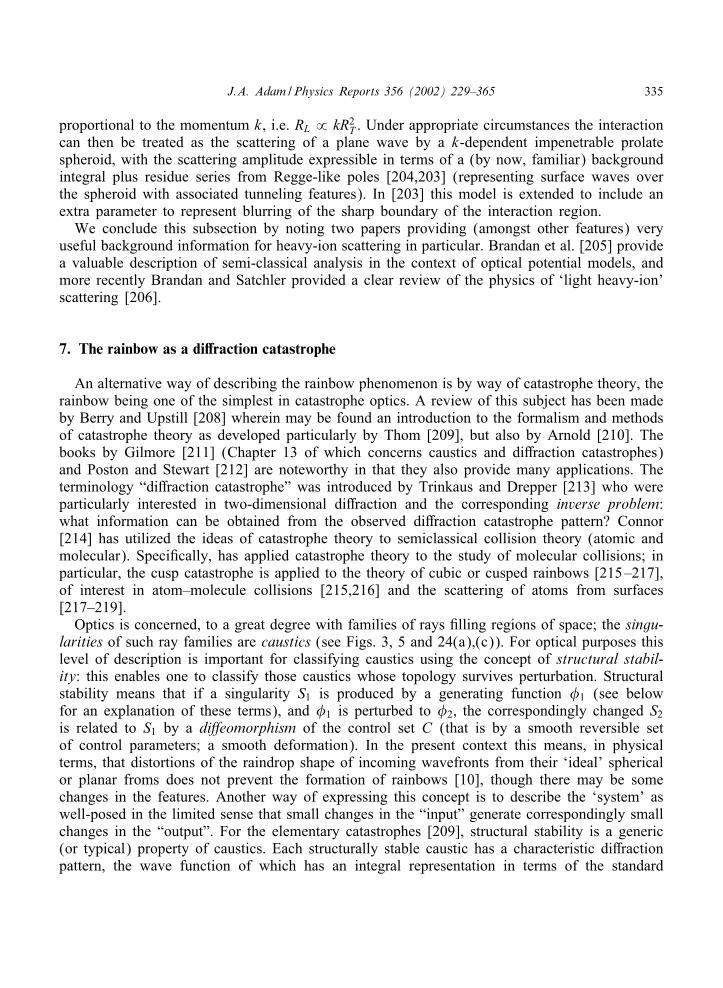
J.A. Adam /Physics Reports 356 (2002) 229–365 335
proportional to the momentum k, i.e. RL ˙ kR2T . Under appropriate circumstances the interaction
can then be treated as the scattering of a plane wave by a k-dependent impenetrable prolatespheroid, with the scattering amplitude expressible in terms of a (by now, familiar) backgroundintegral plus residue series from Regge-like poles [204,203] (representing surface waves overthe spheroid with associated tunneling features). In [203] this model is extended to include anextra parameter to represent blurring of the sharp boundary of the interaction region.
We conclude this subsection by noting two papers providing (amongst other features) veryuseful background information for heavy-ion scattering in particular. Brandan et al. [205] providea valuable description of semi-classical analysis in the context of optical potential models, andmore recently Brandan and Satchler provided a clear review of the physics of ‘light heavy-ion’scattering [206].
7. The rainbow as a di'raction catastrophe
An alternative way of describing the rainbow phenomenon is by way of catastrophe theory, therainbow being one of the simplest in catastrophe optics. A review of this subject has been madeby Berry and Upstill [208] wherein may be found an introduction to the formalism and methodsof catastrophe theory as developed particularly by Thom [209], but also by Arnold [210]. Thebooks by Gilmore [211] (Chapter 13 of which concerns caustics and di9raction catastrophes)and Poston and Stewart [212] are noteworthy in that they also provide many applications. Theterminology “di9raction catastrophe” was introduced by Trinkaus and Drepper [213] who wereparticularly interested in two-dimensional di9raction and the corresponding inverse problem:what information can be obtained from the observed di9raction catastrophe pattern? Connor[214] has utilized the ideas of catastrophe theory to semiclassical collision theory (atomic andmolecular). SpeciAcally, has applied catastrophe theory to the study of molecular collisions; inparticular, the cusp catastrophe is applied to the theory of cubic or cusped rainbows [215–217],of interest in atom–molecule collisions [215,216] and the scattering of atoms from surfaces[217–219].
Optics is concerned, to a great degree with families of rays Alling regions of space; the singu-larities of such ray families are caustics (see Figs. 3, 5 and 24(a),(c)). For optical purposes thislevel of description is important for classifying caustics using the concept of structural stabil-ity: this enables one to classify those caustics whose topology survives perturbation. Structuralstability means that if a singularity S1 is produced by a generating function ,1 (see belowfor an explanation of these terms), and ,1 is perturbed to ,2; the correspondingly changed S2is related to S1 by a di;eomorphism of the control set C (that is by a smooth reversible setof control parameters; a smooth deformation). In the present context this means, in physicalterms, that distortions of the raindrop shape of incoming wavefronts from their ‘ideal’ sphericalor planar froms does not prevent the formation of rainbows [10], though there may be somechanges in the features. Another way of expressing this concept is to describe the ‘system’ aswell-posed in the limited sense that small changes in the “input” generate correspondingly smallchanges in the “output”. For the elementary catastrophes [209], structural stability is a generic(or typical) property of caustics. Each structurally stable caustic has a characteristic di9ractionpattern, the wave function of which has an integral representation in terms of the standard
336 J.A. Adam /Physics Reports 356 (2002) 229–365
polynomial describing the corresponding catastrophe. From a mathematical point of view thesedi9raction catastrophes are especially interesting because they constitute a new hierarchy offunctions, distinct from the special functions of analysis [208].
Before summarizing the mathematical details necessary for the purposes of this review, it isappropriate to discuss in qualitative terms the basic rainbow di9raction catastrophe. As knownfrom geometrical optics, the scattering deviation angle D has a minimum corresponding tothe rainbow angle (or D7escartes ray) when considered as a function of the angle of inci-dence i. Clearly the point (i; D(i)) corresponding to this minimum is a singular point (approxi-mately (59◦; 138◦)) insofar as it separates a two-ray region (D¿Dmin) from a zero-ray region(D¡Dmin) at this geometrical-optics level of description. This is a singularity or caustic point.The rays form a directional caustic at this point, and this is a fold catastrophe (symbol: A2),the simplest example of a catastrophe (see Fig. 24(a); however, it has been noted by McDonald[37] that the caustic is more complicated inside the drop than had previously been realized: thewavefront locus exhibits an odd cusp on a segment of the virtual caustic lying wholly withinthe raindrop). It is the only stable singularity with codimension one (the dimensionality of thecontrol space (one) minus the dimensionality of the singularity itself, which is zero). In spacethe caustic surface is asymptotic to a cone with semiangle 42◦ (see Fig. 24(c)). Alternatively,as in [208], one can regard i as a state (or behavior) variable and D as a control variable; i(D)is of course multivalued (or not a function, depending on one’s preference); and it seems morecausally appropriate to consider D as the state variable.
Di9raction is discussed in [208] in terms of the scalar Helmholtz equation
∇2 (R) + A2N 2(R) (R)=0 (7.1)
for the complex scalar wavefunction (R): The concern in catastrophe optics is to study theasymptotic behavior of wave Aelds near caustics in the short-wave limit A → ∞ (semi-classicaltheory). In a standard manner, (R) is expressed as
(R)= a(R)eiA4(R) ; (7.2)
where the modulus a and the phase A4 are both real quantities. To the lowest order of approx-imation 4 satisAes the Hamilton–Jacobi equation and can be determined asymptotically interms of a phase-action exponent (surfaces of constant action are the wavefronts of geometricaloptics). The integral representation for is
(R)= e−in�=4( A2�
)n=2 ∫: : :∫
b(s;R) exp[iA,(s;R)] dns ; (7.3)
where n is the number of state (or behavior) variables s and b is a weight function. In generalthere is a relationship between this representation and the simple ray approximation (see [208]for further details). According to the principle of stationary phase, the main contributions tothe above integral for given R come from the stationary points, i.e. those points si for whichthe gradient map 9,=9si vanishes; caustics are singularities of this map, where two or morestationary points coalesce. Because A → ∞, the integrand is a rapidly oscillating function of sso other than near the points si, destructive interference occurs and the corresponding contribu-tions are negligible. The stationary points are well separated provided R is not near a caustic;
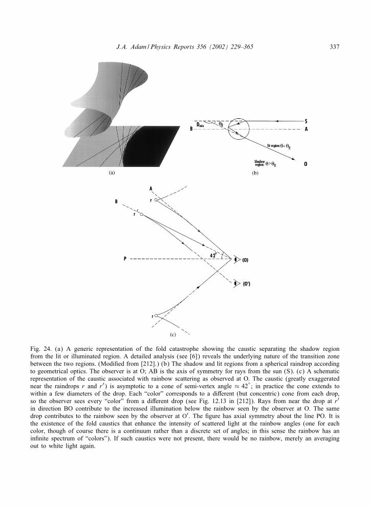
J.A. Adam /Physics Reports 356 (2002) 229–365 337
Fig. 24. (a) A generic representation of the fold catastrophe showing the caustic separating the shadow regionfrom the lit or illuminated region. A detailed analysis (see [6]) reveals the underlying nature of the transition zonebetween the two regions. (ModiAed from [212].) (b) The shadow and lit regions from a spherical raindrop accordingto geometrical optics. The observer is at O; AB is the axis of symmetry for rays from the sun (S). (c) A schematicrepresentation of the caustic associated with rainbow scattering as observed at O. The caustic (greatly exaggeratednear the raindrops r and r′) is asymptotic to a cone of semi-vertex angle ≈ 42
◦; in practice the cone extends to
within a few diameters of the drop. Each “color” corresponds to a di9erent (but concentric) cone from each drop,so the observer sees every “color” from a di9erent drop (see Fig. 12:13 in [212]). Rays from near the drop at r′in direction BO contribute to the increased illumination below the rainbow seen by the observer at O. The samedrop contributes to the rainbow seen by the observer at O′. The Agure has axial symmetry about the line PO. It isthe existence of the fold caustics that enhance the intensity of scattered light at the rainbow angles (one for eachcolor, though of course there is a continuum rather than a discrete set of angles; in this sense the rainbow has aninAnite spectrum of “colors”). If such caustics were not present, there would be no rainbow, merely an averagingout to white light again.
338 J.A. Adam /Physics Reports 356 (2002) 229–365
the simplest form of stationary phase can then be applied, and yields a series of terms of theform
(R) ≈∑P
aP exp[igP(A;R)] ; (7.4)
where the details of the gP need not concern us here. Near a caustic, however, two or moreof the stationary points are close (in some appropriate sense) and their contributions cannot beseparated without a reformulation of the stationary phase principle to accommodate this (i.e.via the CFU method [72]), or by using di9raction catastrophes. The problem is that the “ray”contributions can no longer be considered separately; when the stationary points approach closerthan a distance O(A−1=2) the contributions are not separated by a region in which destructiveinterference occurs. When such points coalesce, ,(s;R) is stationary to higher than Arst order,and quadratic terms as well as linear terms in s − sP vanish. This implies the existence of aset of displacements dsi, away from the extrema sP, for which the gradient map 9,=9si stillvanishes, i.e. for which∑
i
92,9si9sj
dsi =0 : (7.5)
The condition for this homogeneous system of equations to have a solution (i.e. for the set ofcontrol parameters C to lie on a caustic) is that the Hessian
H (,) ≡ det(92,9si9sj
)=0 ; (7.6)
at points sP(C) where 9,=9si =0 (again, details can be found in [208]). The caustic deAnedby H =0 determines the bifurcation set for which at least two stationary points coalesce (inthe present circumstance this is just the rainbow angle). In view of this discussion there aretwo other ways of expressing this: (i) rays coalesce on caustics, and (ii) caustics correspond tosingularities of gradient maps.
To remedy this problem the function , is replaced by a simpler “normal form” Q with thesame stationary-point structure; the resulting di9raction integral is evaluated exactly. This iswhere the property of structural stability is so important, because if the caustic is structurallystable it must be equivalent to one of the catastrophes (in the di9eomorphic sense describedabove). The result is a generic di9raction integral which will occur in many di9erent contexts.The basic di9raction catastrophe integrals (one for each catastrophe) may be reduced to theform
M(C)=1
(2�)n=2
∫: : :∫
exp[iQ(s;C)] dns ; (7.7)
where s represents the state variables and C the control parameters (for the case of the rainbowthere is only one of each, so n=1). These integrals stably represent the wave patterns nearcaustics. The corank of the catastrophe is equal to n: it is the minimum number of statevariables necessary for Q to reproduce the stationary-point structure of ,; the codimension isthe dimensionality of the control space minus the dimensionality of the singularity itself. It is

J.A. Adam /Physics Reports 356 (2002) 229–365 339
interesting to note that in “ray” catastrophe optics the state variables s are removed by di9eren-tiation (the vanishing of the gradient map); in “wave” catastrophe optics they are removed byintegration (via the di9raction functions). For future reference we state the functions Q(s;C)for both the fold (A2) and the cusp (A3) catastrophe; the list for the remaining Ave elementarycatastrophes can be found in Table 1 of [208]. For the fold
Q(s;C)= 13s
3 + Cs (7.8)
and for the cusp
Q(s;C)= 14s
4 + 12C2s2 + C1s : (7.9)
As emphasized in [208], the di9raction catastrophes M(C) provide transitional approximations,valid close to the caustic and for short waves. They are increasingly inaccurate far from thecaustic, but the theory of uniform approximation (mentioned throughout this review but initiallyin Section 4 regarding the work of Berry on semi-classical scattering [68]) can be obtained bydeforming the standard integrals (see references in [208] for further details). The technique ismore general than catastrophe optics, since it can be applied to structurally unstable caustics,the glory being an example, the codimension of which is inAnite [208]. This last statementneeds some clariAcation. Because (i) the wavefront associated with the glory possesses circularsymmetry, and (ii) there is an inAnite number of topologically di9erent ways in which the(continuous group) symmetry of a circle may be broken, it follows that in order to And all thestructurally stable caustics “near” the glory requires inAnitely many parameters [220]; indeed,the singularity index R (see below) for the glory is 1
2 which means that it is a stronger singularitythan the elementary catastrophes with codimensions 1–3 (see the table in Section 3 of [220]).The forward di9raction peak from localized scattering objects is an even stronger structurallyunstable caustic than the glory; for further details on short-wave Aelds and Thom’s theorem,again refer to [220].
By substituting the cubic term (7.8) into (7.7) we see that
M(C)=1√2�
∫ ∞
−∞exp[i(s3=3 + Cs)] ds=
√2�Ai(C) ; (7.10)
which has been encountered several times before! For C ¡ 0 there are two rays (stationarypoints of the integrand) whose interference causes oscillations in M(C); for C ¿ 0 there is one(complex) ray that monotonically and exponentially decays to zero. This describes di9ractionnear a fold caustic. Some 50 years after Airy introduced this function [21] to study di9ractionalong the asymptote of a caustic (although he did not express it in these terms), and provideda fundamental description of the supernumerary bows, Larmor [221] obtained power laws forthe variation of fringe spacing with wavelength of light and the curvature of the caustic. Notethat the corresponding integral for the cusp catastrophe is frequently referred to as the Pearceyintegral (based on [222]). The scaling properties found by Airy for the intensity near the causticand by Larmor for the fringe spacing can be deduced by considering, from (7.3) the “physical”
340 J.A. Adam /Physics Reports 356 (2002) 229–365
fold di9raction catastrophe
M(C ′)=( A2�
)1=2 ∫ ∞
−∞exp[iA(s′3=3 + C ′s′)] ds′ ; (7.11)
where, following [208], s′ is proportional to distance along the initial wavefront and C ′ isproportional to distance from the fold caustic. Using the scaling As′3 = s3 implies that
M(C ′)=A1=6√
2�
∫ ∞
−∞exp[i(s3=3 + A2=3C ′s)] ds : (7.12)
When this is compared with a suggested scaling law between the physical wave function (C ′)(dependent on physical controls C ′, independent of A, e.g. position or time) and the di9ractioncatastrophe M(C), where C represents the standard control parameters, i.e. in general,
(C ′)=ARM(A−/i ; C ′j) ; (7.13)
then it follows that R= 16 and /1 = − 2
3 . The exponent R is a measure of the divergence of | |as A → ∞ at the most singular control point C =0 (it is therefore called the singularity index[210]). The /i (there being only one for the rainbow problem) measure the fringe spacings inthe di9erent control directions Cj as A → ∞ [223]. Thus near a fold catastrophe the intensity| |2 is O(A1=3) [21] and the fringe spacing is O(A−2=3) [221]. Note that in contrast to [208] theexponent of A in the argument of M here is negative; it is written in this way without loss ofgenerality.
It is noted in [208] that wavelength scaling laws outside catastrophe optics do not necessarilyfollow the functional form (7.13), an example being the glory (Section 3). As noted in thatsection, the glory, crudely put, is a result of the intense backscattering of light from sphericalwater droplets. For refractive indices
√26N6 2 (obviously excluding water) rays emerging in
the backward direction after one or more internal reTections would form a (structurally unstable)focal line extending to inAnity with intensity | |2 ˙ A. For water a tangentially-incident rayemerges after one internal reTection at an angle of 14◦ to the backward direction with amplitudeO(A−1=6). These surface waves creep around the surface of the drop by di9raction, su9eringwavelength-dependent attenuation as they do so. These rays deAne a focal line, giving rise toa backscattered wave amplitude [6,208]
| |˙ A1=3 exp[− h(Aa)1=3] ; (7.14)
where a is the drop radius and h is a constant. Note that the glory disappears in the geometrical-optics limit.
A very interesting set of papers published by Marston and coworkers [224–228] take theseideas to the next level: generalized rainbows arising via the cusp di9raction catastrophe forscattering from spheroidal drops (see also [229] for a more classical approach to rainbowscattering). Using acoustically levitated drops whose shapes were closely approximated by oblatespheroids with the short (symmetry) axis vertical. These drops were observed to scatter in thehorizontal rainbow region with patterns corresponding to the hyperbolic–umbilic di;ractioncatastrophe (in Arnold’s classiAcation, D+
4 ). An important parameter is the axis ratio q=D=Hwhere D is the diameter in the horizontal plane, and H is in the vertical plane. For q suYcientlyclose to unity, the fold di9raction catastrophe (A2) is observed, as expected. As q increases, a
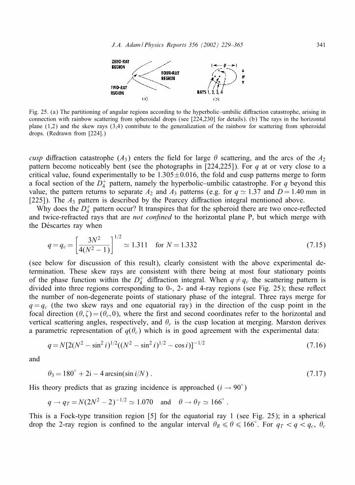
J.A. Adam /Physics Reports 356 (2002) 229–365 341
Fig. 25. (a) The partitioning of angular regions according to the hyperbolic–umbilic di9raction catastrophe, arising inconnection with rainbow scattering from spheroidal drops (see [224,230] for details). (b) The rays in the horizontalplane (1,2) and the skew rays (3,4) contribute to the generalization of the rainbow for scattering from spheroidaldrops. (Redrawn from [224].)
cusp di9raction catastrophe (A3) enters the Aeld for large � scattering, and the arcs of the A2pattern become noticeably bent (see the photographs in [224,225]). For q at or very close to acritical value, found experimentally to be 1:305±0:016, the fold and cusp patterns merge to forma focal section of the D+
4 pattern, namely the hyperbolic–umbilic catastrophe. For q beyond thisvalue, the pattern returns to separate A2 and A3 patterns (e.g. for q � 1:37 and D=1:40 mm in[225]). The A3 pattern is described by the Pearcey di9raction integral mentioned above.
Why does the D+4 pattern occur? It transpires that for the spheroid there are two once-reTected
and twice-refracted rays that are not con?ned to the horizontal plane P, but which merge withthe D7escartes ray when
q= qc =[
3N 2
4(N 2 − 1)
]1=2� 1:311 for N =1:332 (7.15)
(see below for discussion of this result), clearly consistent with the above experimental de-termination. These skew rays are consistent with there being at most four stationary pointsof the phase function within the D+
4 di9raction integral. When q �= qc the scattering pattern isdivided into three regions corresponding to 0-, 2- and 4-ray regions (see Fig. 25); these reTectthe number of non-degenerate points of stationary phase of the integral. Three rays merge forq= qc (the two skew rays and one equatorial ray) in the direction of the cusp point in thefocal direction (�; >)= (�c; 0), where the Arst and second coordinates refer to the horizontal andvertical scattering angles, respectively, and �c is the cusp location at merging. Marston derivesa parametric representation of q(�c) which is in good agreement with the experimental data:
q=N [2(N 2 − sin2 i)1=2((N 2 − sin2 i)1=2 − cos i)]−1=2 (7.16)
and
�3 =180◦ + 2i − 4 arcsin(sin i=N ) : (7.17)
His theory predicts that as grazing incidence is approached (i → 90◦)
q → qT =N (2N 2 − 2)−1=2 � 1:070 and � → �T � 166◦ :
This is a Fock-type transition region [5] for the equatorial ray 1 (see Fig. 25); in a sphericaldrop the 2-ray region is conAned to the angular interval �R6 �6 166◦. For qT ¡q¡qc, �c
342 J.A. Adam /Physics Reports 356 (2002) 229–365
corresponds to the merging of rays 1; 3 and 4. As i → 0◦,
q → qL =[
N2N − 2
]1=2; (7.18)
where qL corresponds to a “lips” event [208,230]. The interval qc ¡q¡qL corresponds to themerging of rays 2–4. Both types of merging have been photographically conArmed.
The scaling laws for the intensity (more accurately, irradiance [22]) I at the focal angles ofthe A2; A3 and D+
4 catastrophes are
I ˙(D�
)p(DR
)2(7.19)
for Axed q, where p= 13 ;
12 and 2
3 , respectively, and R is the far Aeld distance. Marston suggeststhat measurements of �c − �R may be used for the inverse problem of determining q, even ifD is not well known, since �c is independent of D��.
A fascinating prediction is made on the basis of the results in these papers: for a low-altitudesun, oblate-shaped drops might exhibit a “cusped rainbow” (A3 focus) in addition to the usualA2 rainbow. It is suggested that this may occur for D & 1:8 mm. Further details concerningcoloration and technical details concerning, for example, the opening rate of the cusp causticmay be found in [226–228], and references therein.
Immediately following (i.e. adjacent to) the paper by Marston and Trinh [224] was oneby Nye [230] who provided further details of the catastrophe-theoretic interpretation of theirexperimental and analytical results. By examining the point of entry of the incident ray a verticaldistance j above the horizontal plane, he shows that to Arst order in j the direction cosines ofthe incident ray, normal to the surface and refracted ray are the following rows of a determinant:∣∣∣∣∣∣∣∣
sin i 0 cos i
0 H=G 1
sin r H=s cos r
∣∣∣∣∣∣∣∣;
where s=D cos r and G is the radius of curvature of the surface in the vertical plane, H 2=2D.For these three directions to be coplanar the determinant must be zero; this condition yields theresult
qc =DH
=sec r=[
3N 2
4(N 2 − 1)
]1=2; (7.20)
which reconArms the analysis of [224]. Nye further predicts the occurrence of a new phe-nomenon (a lips event, in the terminology of [132]) as N → 2. For further details consult thepaper by Nye [230].
When rainbows are viewed in the laboratory at large distances (compared with the size ofthe drop) from single water droplets they are frequently referred to as colored glarespots [231–234]. Lock studied their formation using Mie theory and the results from the complex angularmomentum theory of Nussenzveig [231]. These caustic surfaces are formed by the light rays
J.A. Adam /Physics Reports 356 (2002) 229–365 343
emerging from the droplet and the focusing properties of the eye. Some of the emerging raysin the lit region form a real caustic beginning near the surface of the drop and ending on theD7escartes ray; the remainder, traced backwards, form a virtual caustic on the rear side of thedrop and extending backward with the D7escartes ray as asymptote. These caustics then act asreal or virtual sources of the glare spots. In his paper Lock remarks that when an observer isfar from a droplet, he sees the Mie scattered intensity, whereas close to the droplet he seesthe square of the Fourier transform of the Mie scattered electric Aeld. He suggests that thisFourier-transforming property of the eye may account for the occasional reports of the tertiaryrainbow seen in the atmosphere. Noting that the Mie inAnite series of partial waves is an exactsolution for the scattering of plane electromagnetic waves from a sphere, Lock points out thatall scattering e9ects that can possibly occur are “hidden somewhere or another” in the Mieamplitude. The extraction of this information has been at times problematical, but by Fouriertransforming the Mie Aelds, many signals (with their own periodicity) superposed in the spatialdomain, become separated in the Fourier domain. This helps to determine the properties ofglare spots that are determined by geometrical considerations and those which may not be; inparticular a glare spot produced by rays at grazing incidence appears in the Fourier transformedMie Aelds was noted, the physical mechanism of which was unclear.
8. Summary
In summarizing the di9erent aspects of the rainbow discussed in this review, it seems ap-propriate to identify some categories that, although a little vague and not mutually exclusive,may serve to describe that phenomenon in a variety of di9erent contexts. These are somewhatheuristic in character, but nonetheless may serve as a reminder of the many complementarylevels of description that can be appreciated from the viewpoint of mathematical physics.A rainbow is:
(1) A concentration of light rays corresponding to a minimum (for the primary bow) of thedeviation or scattering angle D(i) as a function of the angle of incidence i; this minimum isidentiAed as the D7escartes or rainbow ray.
(2) A caustic, separating a 2-ray region from a 0-ray (or shadow) region.(3) An integral superposition of waves over a (locally) cubic wavefront (the Airy approxi-
mation).(4) In part, an interference problem (the origin of the supernumerary bows).(5) A coalescence of two real saddle points.(6) (i) A result of scattering by (or interactions with) an e9ective potential comprising a
square well and a centrifugal barrier.(6) (ii) An example of Regge-pole dominance.(7) Associated with tunneling in the edge domain (see Section 5.6 and Fig. 13).(8) DeAned, to a considerable extent by the behavior of the scattering amplitude for the third
term in the Debye series expansion.(9) A tangentially polarized circular arc.(10) A fold di9raction catastrophe.
344 J.A. Adam /Physics Reports 356 (2002) 229–365
Since much of this review is devoted to an exposition of the complex angular momentumtheory of the rainbow (and to a lesser extent the glory), it is of interest also to summarizethe di9erences as well as similarities between the predictions of the Airy theory (of particularhistorical importance) and CAM theory:
8.1. The rainbow according to CAM theory
While conArming some aspects of the Airy theory, the method of complex angular momentumpredicts di9erences also: six major features of the CAM theory are summarized in [10]:
(i) Rainbow enhancement: The scattering amplitudes predicted by geometrical optics (thezeroth-order WKB term) are O(); CAM theory predicts O(7=6), or a maximum rainbowintensity enhancement of O(1=3), in agreement with the Airy theory.
(ii) Rainbow width: The angular width is O(62), much narrower than the penumbral angularwidth of O(6); hence only a fraction of the total scattered intensity “inhabits” a rainbow.
(iii) Rainbow polarization: CAM theory predicts that the parallel polarization intensity isabout 4% of the corresponding ‘perpendicular’ one; thus there is almost complete dominanceof the latter (for which the electric Aeld vector is tangential to the rainbow arc) in agree-ment with observations [146,147]. While this is basically consistent with the Airy theory,there are deviations from the latter as functions of the angle of observation and the sizeparameter.
(iv) Angular distribution and supernumerary peaks: The Airy theory is valid only for largesize parameters and small deviations from �R, within the rainbow peak. Corrections to thetheory are nevertheless small here, however, for the perpendicular polarization, only becomingsigniAcant for the supernumeraries. Large deviations occur for the parallel polarization becauseof the dominance of a term involving the derivative of the Airy function Ai. Indeed, CAM theorypredicts (correctly, see [127]) that the peaks for the parallel polarization are located near theminima for the perpendicular component, and vice-versa (because constructive interference forthe latter become destructive for the former, the reTection amplitudes for the parallel polarizationchange sign after going through zero at the Brewster angle).
(v) Uniform approximation: The dominant contribution to the third Debye term in the rain-bow region is a uniform asymptotic expansion. On the bright side of the rainbow, this resultmatches smoothly with the WKB approximation in the 2-ray region. On the dark side, it does soagain, this time with the damped complex saddle-point contribution. Put di9erently, di9ractioninto the shadow side of a rainbow occurs by tunneling.
(vi) Higher-order rainbows: The uniform CAM theory can be extended naturally to higher-order bows. For a Debye term of order p, the critical angle of incidence for a rainbow is, (fromEq. (1.3), where p= k + 1)
ip =arccos(N 2 − 1p2 − 1
)1=2:
This angle increases monotonically with p, so that higher-order rainbows arise from incidencewithin the edge strip. Note also that, since the angular width of the rainbow is O(p2=3), i.e.growing linearly with p for large values of p, the rainbow peak Tattens with increasing p
J.A. Adam /Physics Reports 356 (2002) 229–365 345
values. Interestingly, while the intensity of higher-order rainbows decreases with p by virtue oflosses by internal reTection, this becomes less pronounced as p increases because the reTectivityincreases as the edge is approached. The deviations from the Airy theory increase with p forboth polarizations.
In many respects, the rainbow is, in physical terms at least, a simpler phenomenon than theglory. Khare and Nussenzveig [47] list eight di9erent physical e9ects which together or in partcan contribute to this second beautiful occurrence. These are:
(i) The edge e;ect: This is the e9ect of incident rays in the domain (again, see Section 5.5and Fig. 13). These rays are both above and below the barrier of the e9ective potential in thisdomain, and correspond, respectively, to rays that are incident on the drop from within the Fockpenumbral region, and rays that reach the surface by tunneling (barrier penetration).
(ii) “Orbiting”: This applies to rays that penetrate the drop at angles close to critical; theyundergo nearly total internal reTection and consequently are able to make many circumlocutionswithin the drop with appreciable damping. Mathematically, many higher-order Debye termscontribute to this e9ect.
(iii) Axial focusing: The axial symmetry of the problem and the peripheral nature of theleading contributions to the glory give rise to an amplitude enhancement ∼ 1=2.
(iv) Cross-polarization: This occurs because of interference between contributions of compa-rable magnitude from the electric and magnetic polarization components, leading to additionalstructure in the glory pattern.
(v) Surface waves: These represent one of the two categories of leading contributions to theglory (the other being complex rainbow rays: see (vi) below). These arise from Regge–Debyepoles. In addition to strictly surface waves, waves that subsequently take (or have previouslytaken) additional shortcuts through the drop also must be accounted for. A limiting case is a“glory ray” contribution, an example of which is the p=24 case for N given by Eq. (6.4),which yields a Fock-type term (see Fig. 21).
(vi) Complex rainbow rays: These arise on the shadow side of higher-order rainbows formednear the backward direction (for a description of these higher-order rainbows and their locationrelative to the observer see [14,132,133]). Mathematically, they are complex saddle points andphysically they occur because of the 1=6 rainbow enhancement factor [61] and the Tatteningof the rainbow peak for higher-order rainbows.
(vii) Geometrical resonances: These are closed (or nearly so) quasi-periodic orbits associatedwith both the quasi-periodicity of the glory pattern and the narrow resonances or “spikes”. Suchorbits play an important role in the semi-classical description of quantization, and the study ofresonances and bound states [235].
(viii) Competitive damping: In general, the glory pattern and its polarization are functionsof both and �, reTecting the interplay between several competing damping e9ects. The out-come of such competition determines whether or not the leading term is electric or mag-netic in character, surface-wave or rainbow-type, and the ordering of Debye contributions.The di9erent types of damping have been noted earlier: surface waves are radiation-dampedin tangential directions; rainbow terms are damped as complex rays in the shadow of acaustic; and all terms are subject to damping as a result of multiple internal reTections.For ∼ 102 surface-wave e9ects are generally dominant; rainbow e9ects are dominant for∼ 103.
346 J.A. Adam /Physics Reports 356 (2002) 229–365
In [47] the authors make an important point in connection with these many di9erent typesof contribution (see also [235–237]):
“The glory shows for the Arst time in optics that di9raction e9ects due to complex or-bits (surface waves, complex rainbow rays) may be strongly dominant over geometricaloptic ray contributions (real orbits). The moral this suggests is that complex extremals ofFeynman path integrals may have to be taken into account in more general situations.”
Continuing this theme, at the end of his book [10] Nussenzveig asks the question (raisedat the beginning of this article): why complex angular momentum? He draws the conclusionthat, in part at least, it is because of the intimate relationship that exists between tunnelingand analytic continuation, noting that all descriptions of the former make use of the latter (inone form or another). It is perhaps surprising, initially, that such ‘physical’ and ‘mathematical’topics should be so closely related, but a moment’s reTection on both the historical and currentrelationship between the two subjects indicates that this is fascinating but very natural. Indeed,to quote from [10]:
“Ultimately, this [relationship] goes back to Euler’s great discovery of the connectionbetween oscillations and the exponential function, exempliAed by what has been called oneof the most beautiful formulas of mathematics, his synthesis of analysis, algebra, geometryand arithmetic: ei� =− 1.”
It is Atting that “one of the most beautiful formulas of mathematics” should provide the basisfor a richer understanding of two of the most beautiful meteorological phenomena known.Nussenzveig explains further why CAM theory is especially well suited to the treatment ofsemiclassical problems:
“angular momentum is conjugate to the scattering angle, and the localization principleprovides a natural physical interpretation of the Poisson representation, linking Huygens’principle with pseudoclassical paths. This allows one to combine physical insights derivedfrom classical wave theory and from quantum potential scattering in order to deal withpreviously intractable dynamical features of di9raction.
Thus, the beautiful mathematical theory of analytical continuation provides the key toa deeper understanding of some of the most beautiful phenomena displayed in the sky,and also manifested in so many other ways—through all scales of size—revealing theunderlying unity of nature.”
It is quite remarkable that, despite the tremendous development of mathematical physics sincethe time of Newton, he was able to express similar thoughts almost 300 years earlier when hestated in ‘Question 31’ of “Opticks” that
“Nature is very consonant and conformable to herself.” [241]
Acknowledgements
It is a pleasure to acknowledge the assistance of several individuals during the preparationof this manuscript. In particular, I am grateful to Professor H.M. Nussenzveig for permission
J.A. Adam /Physics Reports 356 (2002) 229–365 347
to use some Agures from some of his publications; I have found the book [10] to be a valuableresource, especially with regard to what one might describe as ‘macroscopic tunneling’, but alsoas a source of references to rainbows and glories in atomic, molecular and nuclear scattering.I am also grateful to Professor M.S. Hussein who provided me with references to some ofhis most recent publications. Both the anonymous reviewer and the editor, Professor J. Eichlerprovided valuable feedback and advice which helped to improve the manuscript considerably.In addition, Professor T.F. Gallagher o9ered advice in the early stages of preparation of thisarticle. My colleague Professor Mark Lesley drew my attention to the statement by Newton(quoted above); I am delighted that his enthusiasm for this project has been almost as great asmine. Finally I would like to thank all the sta9 at the editorial oYce in Amsterdam, particularlyYvonne van Lieshout who patiently encouraged me through the entire editorial process.
Appendix A. Classical scattering; the scattering cross section
Consider the problem of a particle of mass m moving under the inTuence of a central Aeld;the path of the particle lies in one plane and its angular momentum M is conserved [238,239],i.e. in standard notation,
M =mr2�=constant : (A.1)
It is well-known that this implies Kepler’s second law, namely that the radius vector of theparticle sweeps out equal areas in equal times. If V (r) is the potential Aeld in which the particlemoves, then the total energy E of the particle may be written as
E = 12m(r2 + r2�
2) + V (r)= 1
2mr2 +M 2
2mr2+ V (r) ; (A.2)
from which
r=
√√√√{ 2m
[E − V (r)]−(
Mmr
)2: (A.3)
This expression can be integrated to yield the time t explicitly, or from (A.1)
�=∫
Mr2√
{2m[E − V (r)]− (M=r)2dr + constant ; (A.4)
which is the general solution of the equation of the path �(r). It also follows from (A.1) that� varies monotonically with time since � never changes sign. The quantity
M 2
2mr2+ V (r)=U (r) (A.5)
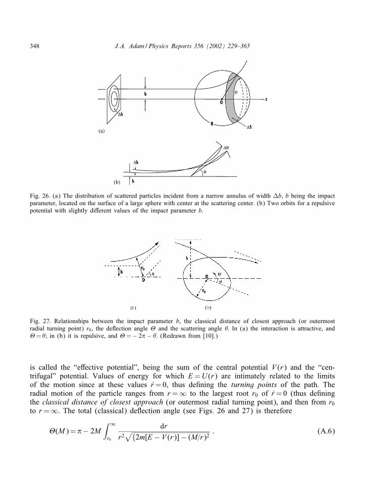
348 J.A. Adam /Physics Reports 356 (2002) 229–365
Fig. 26. (a) The distribution of scattered particles incident from a narrow annulus of width ]b, b being the impactparameter, located on the surface of a large sphere with center at the scattering center. (b) Two orbits for a repulsivepotential with slightly di9erent values of the impact parameter b.
Fig. 27. Relationships between the impact parameter b, the classical distance of closest approach (or outermostradial turning point) r0, the deTection angle @ and the scattering angle �: In (a) the interaction is attractive, and@= �; in (b) it is repulsive, and @= − 2�− �. (Redrawn from [10].)
is called the “e9ective potential”, being the sum of the central potential V (r) and the “cen-trifugal” potential. Values of energy for which E =U (r) are intimately related to the limitsof the motion since at these values r=0, thus deAning the turning points of the path. Theradial motion of the particle ranges from r=∞ to the largest root r0 of r=0 (thus deAningthe classical distance of closest approach (or outermost radial turning point), and then from r0to r=∞. The total (classical) deTection angle (see Figs. 26 and 27) is therefore
@(M)=�− 2M∫ ∞
r0
drr2√
{2m[E − V (r)]− (M=r)2: (A.6)
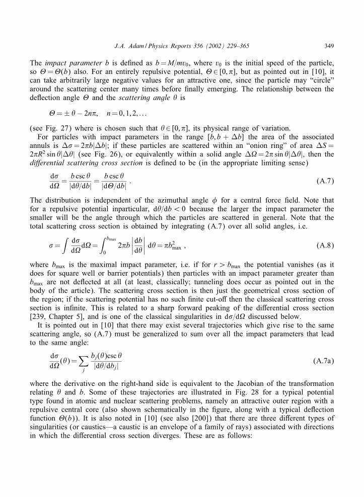
J.A. Adam /Physics Reports 356 (2002) 229–365 349
The impact parameter b is deAned as b=M=mv0, where v0 is the initial speed of the particle,so @=@(b) also. For an entirely repulsive potential, @∈ [0; �], but as pointed out in [10], itcan take arbitrarily large negative values for an attractive one, since the particle may “circle”around the scattering center many times before Anally emerging. The relationship between thedeTection angle @ and the scattering angle � is
@=± �− 2n�; n=0; 1; 2; : : :
(see Fig. 27) where is chosen such that �∈ [0; �], its physical range of variation.For particles with impact parameters in the range [b; b + ]b] the area of the associated
annuls is ]/=2�b|]b|; if these particles are scattered within an “onion ring” of area ]S =2�R2 sin �|]�| (see Fig. 26), or equivalently within a solid angle ]0=2� sin �|]�|, then thedi;erential scattering cross section is deAned to be (in the appropriate limiting sense)
d/d0
=b csc �|d�=db| =
b csc �|d@=db| : (A.7)
The distribution is independent of the azimuthal angle , for a central force Aeld. Note thatfor a repulsive potential inparticular, d�=db¡ 0 because the larger the impact parameter thesmaller will be the angle through which the particles are scattered in general. Note that thetotal scattering cross section is obtained by integrating (A.7) over all solid angles, i.e.
/=∫
d/d0
d0=∫ bmax
02�b
∣∣∣∣dbd�∣∣∣∣ d�=�b2
max ; (A.8)
where bmax is the maximal impact parameter, i.e. if for r¿bmax the potential vanishes (as itdoes for square well or barrier potentials) then particles with an impact parameter greater thanbmax are not deTected at all (at least, classically; tunneling does occur as pointed out in thebody of the article). The scattering cross section is then just the geometrical cross section ofthe region; if the scattering potential has no such Anite cut-o9 then the classical scattering crosssection is inAnite. This is related to a sharp forward peaking of the di9erential cross section[239, Chapter 5], and is one of the classical singularities in d/=d0 discussed below.
It is pointed out in [10] that there may exist several trajectories which give rise to the samescattering angle, so (A.7) must be generalized to sum over all the impact parameters that leadto the same angle:
d/d0
(�)=∑j
bj(�)csc �|d�=dbj| (A.7a)
where the derivative on the right-hand side is equivalent to the Jacobian of the transformationrelating � and b. Some of these trajectories are illustrated in Fig. 28 for a typical potentialtype found in atomic and nuclear scattering problems, namely an attractive outer region with arepulsive central core (also shown schematically in the Agure, along with a typical deTectionfunction @(b)). It is also noted in [10] (see also [200]) that there are three di9erent types ofsingularities (or caustics—a caustic is an envelope of a family of rays) associated with directionsin which the di9erential cross section diverges. These are as follows:
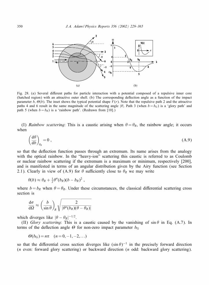
350 J.A. Adam /Physics Reports 356 (2002) 229–365
Fig. 28. (a) Several di9erent paths for particle interaction with a potential composed of a repulsive inner core(hatched region) with an attractive outer shell. (b) The corresponding deTection angle as a function of the impactparameter b; @(b): The inset shows the typical potential shape V (r): Note that the repulsive path 2 and the attractivepaths 4 and 6 result in the same magnitude of the scattering angle |�|. Path 3 (when b= bG) is a ‘glory path’ andpath 5 (when b= bR) is a ‘rainbow path’. (Redrawn from [10].)
(I) Rainbow scattering: This is a caustic arising when �= �R, the rainbow angle; it occurswhen (
d�db
)�R
=0 ; (A.9)
so that the deTection function passes through an extremum. Its name arises from the analogywith the optical rainbow. In the “heavy-ion” scattering this caustic is referred to as Coulombor nuclear rainbow scattering if the extremum is a maximum or minimum, respectively [200],and is manifested in terms of an angular distribution given by the Airy function (see Section2.1). Clearly in view of (A.9) for � suYciently close to �R we may write
�(b) ≈ �R + 12�
′′(bR)(b− bR)2 ;
where b= bR when �= �R. Under these circumstances, the classical di9erential scattering crosssection is
d/d0
≈(
bsin �
)R
√2
|�′′(bR)(�− �R)|
which diverges like |�− �R|−1=2.(II) Glory scattering: This is a caustic caused by the vanishing of sin � in Eq. (A.7). In
terms of the deTection angle @ for non-zero impact parameter bG
@(bG)= n� (n=0;−1;−2; : : :)
so that the di9erential cross section diverges like (sin �)−1 in the precisely forward direction(n even: forward glory scattering) or backward direction (n odd: backward glory scattering).
J.A. Adam /Physics Reports 356 (2002) 229–365 351
Eq. (A.6) implies that @=� can only occur when b=0; this case does not constitute gloryscattering. The characteristic angular distribution behaves like a zeroth-order Bessel function[200], where it is pointed out that nuclear rainbow scattering and backward glory scattering areexpected to be good probes of nuclear interaction at relatively short distances, as is forwardglory scattering at relatively large distances.
(III) Forward peaking: As alluded to above, scattering potentials with tails extending asymp-totically to zero at inAnity will lead in general to a divergent forward di9erential cross section.This is because of the accumulation of small deTections for particles with arbitrarily largeimpact parameters, i.e. from (A.7a) in which some bj → ∞; � → 0 while |d�=dbj| remainsbounded. Even for cut-o9 potentials, some forward anomaly is still to be expected. There is afourth situation that may occur when the e9ective potential U (r)=UM (r) for a given value ofM has a relative maximum at r= r0:
(IV) Orbiting: In this case
UM (r)=E; (dUM=dr)r0 = 0 :
This is interpreted as the existence of an unstable circular orbit with radius r0 [10]. Underthese circumstances the integral (A.6) diverges logarithmically at its lower limit if U ′′
M (r0) �=0.A simple calculation yields the result that @(M) → −∞ as r → r0; this means that a particlewith this energy and angular momentum will spiral indeAnitely around the scattering center,and taking an inAnitely long time to reach the top of the “barrier”. In addition, the inversefunction b(�) becomes inAnitely many-valued, so an inAnite number of branches contribute tothe di9erential cross section (A.7a). If UM (r) has a local minimum for r¡r0 then particles withenergy E¡UM (r0) can sustain oscillatory orbits within the potential “well”, and the unstablecircular orbit functions as a separatrix between bounded and unbounded trajectories [10] (seealso [240]). Fig. 29 illustrates connections between the e9ective potential, tunneling and the raypicture in rainbow and glory formation.
A.1. Semi-classical considerations: a prBecis
In a sense, the semi-classical approach is the “geometric mean” between classical and quan-tum mechanical descriptions of phenomena; while one wishes to retain the concept of particletrajectories and their individual contributions, there is nevertheless an associated de Brogliewavelength for each particle, so that interference and di9raction e9ects enter the picture. Thelatter do so via the transition from geometrical optics to wave optics. The di9erential scat-tering cross section is related to the quantum scattering amplitude f(k; �) and this in turn isexpressible as the familiar partial wave expansion [65]. The formal relationship between thisand the classical di9erential cross section is established using the WKB approximation and theprinciple of stationary phase is used to evaluate asymptotically a certain phase integral (see [10,Section 1.2] for further details). A point of stationary phase can be identiAed with a classicaltrajectory, but if more than one such point is present (provided they are well separated andof the Arst order) the corresponding expression for |f(k; �)|2 will contain interference terms.This is a distinguishing feature of the ‘primitive’ semi-classical formulation, and has signiAcantimplications for e9ects (I)–(IV) noted above. The inAnite intensities (incorrectly) predicted
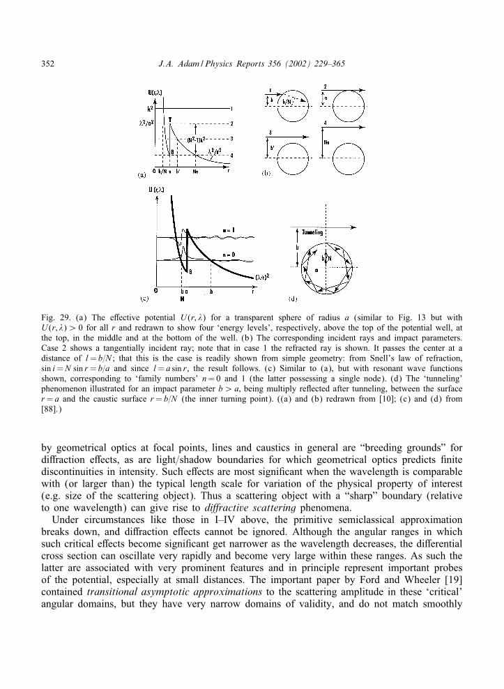
352 J.A. Adam /Physics Reports 356 (2002) 229–365
Fig. 29. (a) The e9ective potential U (r; �) for a transparent sphere of radius a (similar to Fig. 13 but withU (r; �)¿ 0 for all r and redrawn to show four ‘energy levels’, respectively, above the top of the potential well, atthe top, in the middle and at the bottom of the well. (b) The corresponding incident rays and impact parameters.Case 2 shows a tangentially incident ray; note that in case 1 the refracted ray is shown. It passes the center at adistance of l= b=N ; that this is the case is readily shown from simple geometry: from Snell’s law of refraction,sin i=N sin r = b=a and since l= a sin r, the result follows. (c) Similar to (a), but with resonant wave functionsshown, corresponding to ‘family numbers’ n=0 and 1 (the latter possessing a single node). (d) The ‘tunneling’phenomenon illustrated for an impact parameter b¿a; being multiply reTected after tunneling, between the surfacer = a and the caustic surface r = b=N (the inner turning point). ((a) and (b) redrawn from [10]; (c) and (d) from[88].)
by geometrical optics at focal points, lines and caustics in general are “breeding grounds” fordi9raction e9ects, as are light=shadow boundaries for which geometrical optics predicts Anitediscontinuities in intensity. Such e9ects are most signiAcant when the wavelength is comparablewith (or larger than) the typical length scale for variation of the physical property of interest(e.g. size of the scattering object). Thus a scattering object with a “sharp” boundary (relativeto one wavelength) can give rise to di;ractive scattering phenomena.
Under circumstances like those in I–IV above, the primitive semiclassical approximationbreaks down, and di9raction e9ects cannot be ignored. Although the angular ranges in whichsuch critical e9ects become signiAcant get narrower as the wavelength decreases, the di9erentialcross section can oscillate very rapidly and become very large within these ranges. As such thelatter are associated with very prominent features and in principle represent important probesof the potential, especially at small distances. The important paper by Ford and Wheeler [19]contained transitional asymptotic approximations to the scattering amplitude in these ‘critical’angular domains, but they have very narrow domains of validity, and do not match smoothly
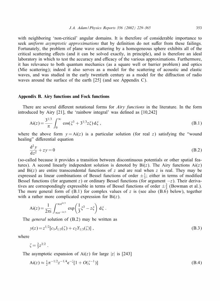
J.A. Adam /Physics Reports 356 (2002) 229–365 353
with neighboring ‘non-critical’ angular domains. It is therefore of considerable importance toseek uniform asymptotic approximations that by deAnition do not su9er from these failings.Fortunately, the problem of plane wave scattering by a homogeneous sphere exhibits all of thecritical scattering e9ects (and it can be solved exactly, in principle), and is therefore an ideallaboratory in which to test the accuracy and eYcacy of the various approximations. Furthermore,it has relevance to both quantum mechanics (as a square well or barrier problem) and optics(Mie scattering); indeed it also serves as a model for the scattering of acoustic and elasticwaves, and was studied in the early twentieth century as a model for the di9raction of radiowaves around the surface of the earth [25] (and see Appendix C).
Appendix B. Airy functions and Fock functions
There are several di9erent notational forms for Airy functions in the literature. In the formintroduced by Airy [21], the ‘rainbow integral’ was deAned as [10,242]
Ai(z)=31=3
�
∫ ∞
0cos(+3 + 31=3z+) d+ ; (B.1)
where the above form y=Ai(z) is a particular solution (for real z) satisfying the “woundhealing” di9erential equation
d2ydz2
+ zy=0 (B.2)
(so-called because it provides a transition between discontinuous potentials or other spatial fea-tures). A second linearly independent solution is denoted by Bi(z). The Airy functions Ai(z)and Bi(z) are entire transcendental functions of z and are real when z is real. They may beexpressed as linear combinations of Bessel functions of order ±1
3 ; either in terms of modiAedBessel functions (for argument z) or ordinary Bessel functions (for argument −z). Their deriva-tives are correspondingly expressible in terms of Bessel functions of order ±2
3 (Bowman et al.).The more general form of (B.1) for complex values of z is (see also (B.6) below), togetherwith a rather more complicated expression for Bi(z).
Ai(z)=1
2�i
∫ ∞ei�=3
∞e−i�=3exp(
13+3 − z+
)d+ :
The general solution of (B.2) may be written as
y(z)= z1=2[c1J1=3(>) + c2Y1=3(>)] ; (B.3)
where
>= 23z
3=2 :
The asymptotic expansion of Ai(z) for large |z| is [243]
Ai(z) ≈ 12�
−1=2z−1=4e−>[1 + O(>−1)] (B.4)
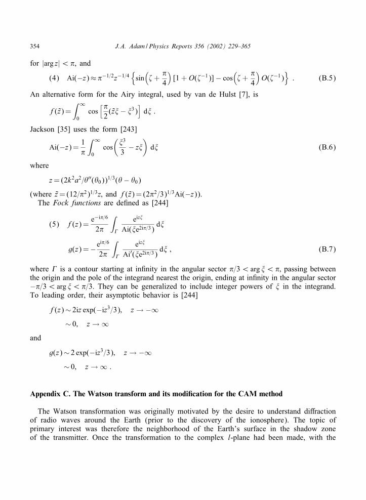
354 J.A. Adam /Physics Reports 356 (2002) 229–365
for |arg z|¡�, and
(4) Ai(−z)≈ �−1=2z−1=4{sin(> +
�4
)[1 + O(>−1)]− cos
(> +
�4
)O(>−1)
}: (B.5)
An alternative form for the Airy integral, used by van de Hulst [7], is
f(z)=∫ ∞
0cos[�2(z+− +3)
]d+ :
Jackson [35] uses the form [243]
Ai(−z)=1�
∫ ∞
0cos(+3
3− z+
)d+ (B.6)
where
z=(2k2a2=�′′(�0))1=3(�− �0)
(where z=(12=�2)1=3z; and f(z)= (2�2=3)1=3Ai(−z)).The Fock functions are deAned as [244]
(5) f(z)=e−i�=6
2�
∫F
eiz+
Ai(+e2i�=3)d+
g(z)=−ei�=6
2�
∫F
eiz+
Ai′(+e2i�=3)d+ ; (B.7)
where F is a contour starting at inAnity in the angular sector �=3¡ arg +¡�; passing betweenthe origin and the pole of the integrand nearest the origin, ending at inAnity in the angular sector−�=3¡ arg +¡�=3. They can be generalized to include integer powers of + in the integrand.To leading order, their asymptotic behavior is [244]
f(z)∼ 2iz exp(−iz3=3); z → −∞∼ 0; z → ∞
and
g(z)∼ 2 exp(−iz3=3); z → −∞∼ 0; z → ∞ :
Appendix C. The Watson transform and its modi.cation for the CAM method
The Watson transformation was originally motivated by the desire to understand di9ractionof radio waves around the Earth (prior to the discovery of the ionosphere). The topic ofprimary interest was therefore the neighborhood of the Earth’s surface in the shadow zoneof the transmitter. Once the transformation to the complex l-plane had been made, with the
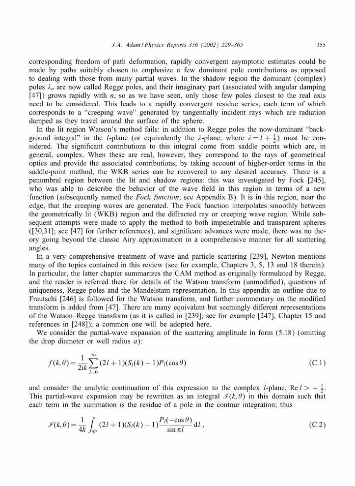
J.A. Adam /Physics Reports 356 (2002) 229–365 355
corresponding freedom of path deformation, rapidly convergent asymptotic estimates could bemade by paths suitably chosen to emphasize a few dominant pole contributions as opposedto dealing with those from many partial waves. In the shadow region the dominant (complex)poles �n are now called Regge poles, and their imaginary part (associated with angular damping[47]) grows rapidly with n, so as we have seen, only those few poles closest to the real axisneed to be considered. This leads to a rapidly convergent residue series, each term of whichcorresponds to a “creeping wave” generated by tangentially incident rays which are radiationdamped as they travel around the surface of the sphere.
In the lit region Watson’s method fails: in addition to Regge poles the now-dominant “back-ground integral” in the l-plane (or equivalently the �-plane, where �= l + 1
2) must be con-sidered. The signiAcant contributions to this integral come from saddle points which are, ingeneral, complex. When these are real, however, they correspond to the rays of geometricaloptics and provide the associated contributions; by taking account of higher-order terms in thesaddle-point method, the WKB series can be recovered to any desired accuracy. There is apenumbral region between the lit and shadow regions: this was investigated by Fock [245],who was able to describe the behavior of the wave Aeld in this region in terms of a newfunction (subsequently named the Fock function; see Appendix B). It is in this region, near theedge, that the creeping waves are generated. The Fock function interpolates smoothly betweenthe geometrically lit (WKB) region and the di9racted ray or creeping wave region. While sub-sequent attempts were made to apply the method to both impenetrable and transparent spheres([30,31]; see [47] for further references), and signiAcant advances were made, there was no the-ory going beyond the classic Airy approximation in a comprehensive manner for all scatteringangles.
In a very comprehensive treatment of wave and particle scattering [239], Newton mentionsmany of the topics contained in this review (see for example, Chapters 3, 5, 13 and 18 therein).In particular, the latter chapter summarizes the CAM method as originally formulated by Regge,and the reader is referred there for details of the Watson transform (unmodiAed), questions ofuniqueness, Regge poles and the Mandelstam representation. In this appendix an outline due toFrautschi [246] is followed for the Watson transform, and further commentary on the modiAedtransform is added from [47]. There are many equivalent but seemingly di9erent representationsof the Watson–Regge transform (as it is called in [239]; see for example [247], Chapter 15 andreferences in [248]); a common one will be adopted here.
We consider the partial-wave expansion of the scattering amplitude in form (5.18) (omittingthe drop diameter or well radius a):
f(k; �)=1
2ik
∞∑l=0
(2l + 1)(Sl(k)− 1)Pl(cos �) (C.1)
and consider the analytic continuation of this expression to the complex l-plane, Re l¿ − 12 :
This partial-wave expansion may be rewritten as an integral I(k; �) in this domain such thateach term in the summation is the residue of a pole in the contour integration; thus
I(k; �)=14k
∫C′
(2l + 1)(Sl(k)− 1)Pl(−cos �)
sin �ldl ; (C.2)
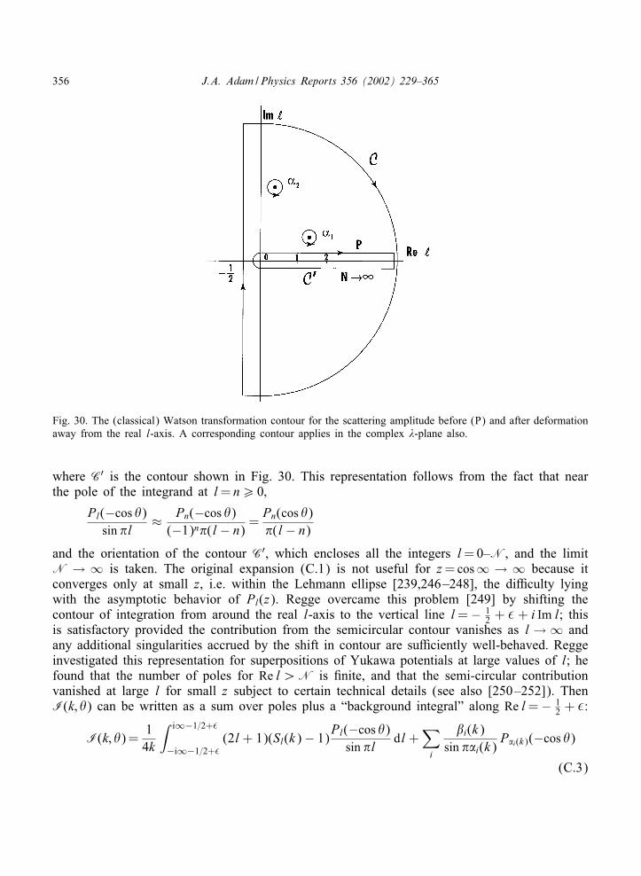
356 J.A. Adam /Physics Reports 356 (2002) 229–365
Fig. 30. The (classical) Watson transformation contour for the scattering amplitude before (P) and after deformationaway from the real l-axis. A corresponding contour applies in the complex �-plane also.
where C′ is the contour shown in Fig. 30. This representation follows from the fact that nearthe pole of the integrand at l= n¿ 0;
Pl(−cos �)sin �l
≈ Pn(−cos �)(−1)n�(l− n)
=Pn(cos �)�(l− n)
and the orientation of the contour C′, which encloses all the integers l=0–N, and the limitN → ∞ is taken. The original expansion (C.1) is not useful for z=cos∞ → ∞ because itconverges only at small z, i.e. within the Lehmann ellipse [239,246–248], the diYculty lyingwith the asymptotic behavior of Pl(z). Regge overcame this problem [249] by shifting thecontour of integration from around the real l-axis to the vertical line l= − 1
2 + j+ i Im l; thisis satisfactory provided the contribution from the semicircular contour vanishes as l → ∞ andany additional singularities accrued by the shift in contour are suYciently well-behaved. Reggeinvestigated this representation for superpositions of Yukawa potentials at large values of l; hefound that the number of poles for Re l¿N is Anite, and that the semi-circular contributionvanished at large l for small z subject to certain technical details (see also [250–252]). ThenI(k; �) can be written as a sum over poles plus a “background integral” along Re l=− 1
2 + j:
I(k; �)=14k
∫ i∞−1=2+j
−i∞−1=2+j(2l + 1)(Sl(k)− 1)
Pl(−cos �)sin �l
dl +∑i
i(k)sin �5i(k)
P5i(k)(−cos �)
(C.3)
J.A. Adam /Physics Reports 356 (2002) 229–365 357
in terms of the pole contributions 5i(k) with factor i. This is sometimes called the Sommerfeld–Watson representation, and now the pole furthest to the right (51 say, with Re l¿− 1
2) dominatesthe integral, i.e. as z=cos � → ∞,
I(k; z) ∼ 1(k)sin �51(k)
z51 : (C.4)
In general, as noted in Section 5, for potentials which are not superpositions of Yukawas(e.g. square well or other Anite-range potentials), the contribution from the semicircular contourdoes not vanish (but see [250]). The Yukawa potentials thus are of great importance for theMandelstam representation [92] (which cannot exist unless I is bounded by a Anite power ofz; (C.4) is also of signiAcance in connection with relativistic scattering [246]).
To elucidate part of the physical signiAcance of (C.3), consider the inner product
Il(k)=12
∫ 1
−1Pl(z)I(k; z) dz ;
along with the relation
12
∫ 1
−1Pl(z)P5(−z) dz=
sin �5�(5− l)(5 + l + 1)
(C.5)
where l is an integer and 5 is complex [243]. (This reduces to the standard result (−1)l=(2l+1)as 5 → l). Consider next the contribution of one Regge pole at l= 5 to Il, namely
(k)�(5(k)− l)(5 + l + 1)
: (C.6)
If 5 ≈ l, this can provide a large contribution which may change rapidly with k (and henceenergy), so if there exists an energy El such that l=Re 5, then expanding 5 in a Taylor seriesabout El yields
5 � l + (E − El)d Re 5(El)
dE+ i Im 5(El) : (C.7)
Then (B.6) can be rewritten in Breit–Wigner form as
�(5 + l + 1)[d Re 5(El)=dE]{E − El + iF=2} (C.8)
where
F2
=Im 5(El)
d Re 5(El)=dE;
I is the resonance half-width. Interpretation of these results to trace the trajectory of the Reggepole may be found in [246,249].
As noted in Section 5, a detailed analysis of a more e9ective version of the Watson trans-formation appeared in 1965 [33], along with many subsequent applications (see Section 5 fordetails). This modi?ed Watson transformation is based on the application of the Poisson sum
358 J.A. Adam /Physics Reports 356 (2002) 229–365
formula [253,254] to the scattering amplitude or the wave Aeld [33]; one form of this formulais:
∞∑l=0
$(l +
12; ; �
)=
∞∑m=−∞
(−1)m∫ ∞
0$(�; ; �) exp(2im��) d� (C.9)
with an appropriate choice of deformed path in the complex �-plane. This choice, which isdi9erent for di9erent angular regions, leads also to Regge pole contributions and saddle-point-dominated background integrals. Khare and Nussenzveig point out that a saddle-point on thereal axis is also a point of stationary phase in (C.9), and this characterizes an extremal path,i.e. a ray in geometrical optics, or a classical orbit in the particle context [47]. The integerm in (C.9) has the topological signiAcance of a winding number, which is associated with thenumber of circumlocutions performed by a path around the center of the sphere. The details andsubtleties of the Regge poles for the problem of scattering by a transparent sphere, the basis ofthe rainbow and the glory, are discussed in detail in Section 5.2, along with the signiAcance ofthe Debye expansion in regaining rapid convergence of the residue series.
A succinct derivation of the Poisson sum formula has been provided in the book by Brink[186], and in view of its importance in CAM theory in particular, the formal proof is presentedhere (in a slightly modiAed form). From the theory of (complex) Fourier series, with standardDirichlet conditions applying to f(x) [255], it follows that
f(x)=∞∑
m=−∞Ame−2m�ix=L ;
where
Am =1L
∫ b+L
bf(�)e2m�i�=L d� :
Note that since m and if l are integers,
f(x + l)=∞∑
m=−∞Ame−2m�ix=Le−2m�ix=L
then choosing L=1 it follows that
f(x + l)=∞∑
m=−∞Ame−2m�ix ;
where
Am =∫ l+1
lf(�)e2m�i� d� ;
having chosen b= l. Therefore in particular
(6) f(l +
12
)=
∞∑m=−∞
Ame−m�i =∞∑
m=−∞(−1)mAm
=∞∑
m=−∞(−1)m
∫ l+1
lf(�)e2m�i� d� : (C.10)
J.A. Adam /Physics Reports 356 (2002) 229–365 359
Hence∞∑l=0
f(l +
12
)=
∞∑m=−∞
(−1)m∞∑l=0
∫ l+1
lf(�)e2m�i� d�=
∞∑m=−∞
(−1)m∫ ∞
0f(�)e2m�i� d�
(C.11)
and all that remains is to replace f(�) by $(�; ; �) to recover (C.9).
Appendix D. The Chester–Friedman–Ursell (CFU) method
This technique is used when two saddle points in the complex �-plane approach one anotheras a parameter governing the conTuence gradually changes. The description given in [10] isfollowed here, notationally adapted to the rainbow problem. The complex integral of interest is
F(; �)=∫
g(�)ef(�; �) d� ; (D.1)
where =2, the asymptotic expansion parameter is large and positive and �= � − �R is anindependent parameter. In the 1-ray region (in particular), the integral is dominated by a singlesaddle-point �= �(�); in the neighborhood of which f and g are regular, so
f(�; �) ≈ f(�; �) + 12f��(�; �)(�− �)2 :
When the path of steepest descent is chosen to pass through �, a Gaussian-type integral occurs,and this yields the dominant contribution to the integral F(; �) in a range ]� about the saddlepoint, where [103]
]� ∼ (|f��(�; �)|)−1=2 :
The asymptotic expansion of F(; �) then follows by standard techniques (a power-seriesexpansion of g about � and subsequent integration term by term [104]).
By contrast, in the 2-ray region there are two saddle points (�′; �
′′say) to be considered,
and provided their ranges do not overlap, their contributions are additive. When the ranges dooverlap, the above method is inapplicable because the series expansion of g has a radius ofconvergence of order |�′ − �
′′|: Furthermore, at conTuence (when �=0), the second derivativef�� is zero, so the second term in f above becomes cubic in �. For a decreasing sequence of?xed � �=0; can be chosen large enough so that the ranges still do not overlap (i.e. ]� → 0 as → ∞), but this does not yield a result uniformly valid in �. Similarly, a cubic approximationfor f(�; �) about �=0 provides only a transitional approximation for F(; �):
The basis of the CFU method is to transform the exponent in the equation (D.1) into anexact cubic by means of the change of variables
f(�; �)= 13u
3 − +(�)u + A(�)
with the two saddle points transformed into ±+1=2(�): The essential feature is to design a map-ping which preserves the saddle point structure [235]. Under these circumstances the mapping
360 J.A. Adam /Physics Reports 356 (2002) 229–365
� ↔ u is analytic and one-to-one near u=0: It follows eventually from (D.1) that an asymptoticexpansion of the following form is valid:
F(; �)= exp[A(�)]
{−1=3
[M−1∑s=0
as(�)−s
+ O(−M
)
]Ai[
2=3+(�)]
+ −2=3
[M−1∑s=0
bs(�)−s
+ O(−M
)
]Ai′[
2=3+(�)]
}:
The as and bs are the so-called ‘CFU coeYcients’ determined from the expansion of the inte-grand after the transformation. When |z|�1 and |arg z|¡�, it is known that [243]
Ai′(z) ≈ −z1=2 Ai(z)
so that the Ai′ corrections in the expression above can become of the same order as the Ai terms.This uniform asymptotic expansion can be matched smoothly with the results from saddle-pointanalysis.
References
[1] K. Sassen, J. Opt. Soc. Am. 69 (1979) 1083.[2] H.M. Nussenzveig, Sci. Am. 236 (1977) 116.[3] M.V. Berry, Sci. Prog. Oxf. 57 (1969) 43.[4] R. Greenler, Rainbows, Halos and Glories, Cambridge University Press, Cambridge, 1980.[5] H.M. Nussenzveig, J. Math. Phys. 10 (1969) 82.[6] H.M. Nussenzveig, J. Math. Phys. 10 (1969) 125.[7] H.C. van de Hulst, Light Scattering by Small Particles, Dover, New York, 1981.[8] R.A.R. Tricker, Introduction to Meteorological Optics, Elsevier, New York, 1970.[9] C.F. Bohren, D.R. Hu9man, Absorption and Scattering of Light by Small Particles, Wiley, New York, 1983.
[10] H.M. Nussenzveig, Di9raction E9ects in Semiclassical Scattering, Cambridge University Press, Cambridge,1992.
[11] C.B. Boyer, The Rainbow, from Myth to Mathematics, Princeton University Press, Princeton, NJ, 1987.[12] N.A. Logan, Proc. IEEE 53 (1965) 773.[13] D.E. Pedgely, Weather 41 (1986) 401.[14] J.D. Walker, Am. J. Phys. 44 (1976) 421.[15] D.K. Lynch, W. Livingston, Color and Light in Nature, Cambridge University Press, New York, 1995.[16] J.D. Austin, F.B. Dunning, Math. Teacher (1988) 484 (September issue); see also S. Janke, UMAP Module
724, COMAP, Inc., Lexington, MA, 1992.[17] R.J. Whitaker, Phys. Teacher 12 (1974) 283.[18] W.J. Humphreys, Physics of the Air, Dover, New York, 1964.[19] K.W. Ford, J.A. Wheeler, Ann. Phys. 7 (1959) 259.[20] E. Hundhausen, H. Pauly, Z. Physik 187 (1965) 305.[21] G.B. Airy, Trans. Camb. Phil. Soc. 6 (1838) 379.[22] G.R. Fowles, Introduction to Modern Optics, Dover, New York, 1975.[23] M. Born, E. Wolf, Principles of Optics, Pergamon, Oxford, 1965.[24] G. Mie, Ann. Physik 25 (1908) 377.[25] G.N. Watson, Proc. R. Soc. A 95 (1918) 83.[26] J. Adam, Phys. Rep. 142 (1986) 263.[27] J. Adam, J. Math. Phys. 30 (1989) 744.
J.A. Adam /Physics Reports 356 (2002) 229–365 361
[28] J. Adam, Wave Motion 12 (1990) 385.[29] C.B. Boyer, Am. J. Phys. 18 (1950) 360.[30] B. Van der Pol, H. Bremmer, Phil. Mag. 24 (1937) 141.[31] B. Van der Pol, H. Bremmer, Phil. Mag. 24 (1937) 825. (See also 25 (1938) 817.)[32] A. Sommerfeld, Partial Di9erential Equations in Physics, Academic Press, New York, 1964 (Appendix II).[33] H.M. Nussenzveig, Ann. Phys. 34 (1965) 23.[34] H.M. Nussenzveig, in: J.E. Bowcock (Ed.), Methods and Problems of Theoretical Physics, North-Holland,
Amsterdam, 1970, p. 203.[35] J.D. Jackson, Phys. Rep. 320 (1999) 27.[36] J.D. Jackson, Classical Electrodynamics, 3rd Edition, Wiley, New York, 1998.[37] J.E. Macdonald, Am. J. Phys. 31 (1963) 282.[38] J.M. Pernter, F.M. Exner, Meteorologische Optik, W. BraumRuller, Vienna, 1910.[39] E. Buchwald, Ann. Phys. 43 (1948) 488.[40] W.V.R. Malkus, R.H. Bishop, R.O. Briggs, NACA Technical Notes 1622 (1948).[41] R. Penndorf, J. Opt. Soc. Am. 52 (1962) 402.[42] R.T. Wang, H.C. van de Hulst, Appl. Opt. 30 (1991) 106.[43] A. Ungut, G. Grehan, G. Gouesbet, Appl. Opt. 20 (1981) 2911.[44] C.W. Querfeld, J. Opt. Soc. Am. 55 (1965) 105.[45] A.J. Patitsas, Can. J. Phys. 50 (1972) 3172.[46] W.J. Wiscombe, Appl. Opt. 19 (1980) 1505.[47] V. Khare, H.M. Nussenzveig, in: U. Landman (Ed.), Statistical Mechanics and Statistical Methods in Theory
and Application, Plenum Press, New York, 1977.[48] H.C. Bryant, N. Jarmie, Ann. Phys. (NY) 47 (1968) 127. See also Chapter 8 in Light from the Sky (readings
from ScientiAc American), Freeman, San Francisco, 1980.[49] G.P. KRonnen, Polarized Light in Nature, Cambridge University Press, Cambridge, 1985.[50] H.C. van de Hulst, J. Opt. Soc. Am. 37 (1947) 16.[51] See M. Born, E. Wolf, Principles of Optics, Pergamon, Oxford, 1965 and references therein.[52] Y.G. Naik, R.M. Joshi, J. Opt. Soc. Am. 45 (1955) 733.[53] V. Khare, in: A.D. Boardman (Ed.), Electromagnetic Surface Modes, Wiley, New York, 1982 (Chapter 11).[54] H.C. Bryant, A.J. Cox, J. Opt. Soc. Am. 56 (1966) 1529.[55] T.S. Fahlen, H.C. Bryant, J. Opt. Soc. Am. 58 (1968) 304.[56] H. Maecker, Ann. Phys. 4 (1948) 409.[57] B.W. Woodward, H.C. Bryant, J. Opt. Soc. Am. 57 (1967) 430.[58] D.S. Langley, M.J. Morrell, Appl. Opt. 30 (1991) 3459.[59] V. Khare, H.M. Nussenzveig, Phys. Rev. Lett. 33 (1974) 976.[60] J.R. Probert-Jones, J. Opt. Soc. Am. A 1 (1984) 822.[61] H.M. Nussenzveig, J. Opt. Soc. Am. 69 (1979) 1068.[62] D.S. Langley, P.L. Marston, Phys. Rev. Lett. 47 (1981) 913.[63] P.L. Marston, D.S. Langley, J. Opt. Soc. Am. 72 (1982) 456.[64] H.M. Nussenzveig, W.J. Wiscombe, Optics Lett. 5 (1980) 455.[65] L.I. Schi9, Quantum Mechanics, 3rd Edition, McGraw-Hill, New York, 1968.[66] K.W. Ford, J.A. Wheeler, Ann. Phys. 7 (1959) 287.[67] H. Bremmer, Terrestrial Radio Waves, Elsevier, Amsterdam, 1949.[68] M.V. Berry, Proc. Phys. Soc. 89 (1966) 479.[69] E.A. Mason, L.J. Monchick, J. Chem. Phys. 41 (1964) 2221.[70] E.A. Mason, R.J. Munn, F.J. Smith, Endeavour 30 (1971) 91.[71] U. Buck, Rev. Mod. Phys. 46 (1974) 369.[72] C. Chester, B. Friedman, F. Ursell, Proc. Camb. Phil. Soc. 53 (1957) 599.[73] M.J. Lighthill, Waves in Fluids, Cambridge University Press, Cambridge, 1987.[74] R.E. Langer, Phys. Rev. 51 (1937) 669.[75] S. Jorna, Proc. R. Soc. A 281 (1964) 99.[76] S.I. Rubinow, Ann. Phys. 14 (1961) 305.

362 J.A. Adam /Physics Reports 356 (2002) 229–365
[77] C.L. Pekeris, Proc. Symp. Appl. Math. 2 (1950) 71.[78] E.T. Copson, Asymptotic Expansions, Cambridge University Press, Cambridge, 1965.[79] N.F. Mott, H.S.W. Massey, The Theory of Atomic Collisions, 2nd Edition, Clarendon Press, Oxford, 1949.[80] E.A. Remler, Phys. Rev. A 3 (1971) 1949.[81] W.G. Rich, S.M. Bobbio, R.L. Champion, L.D. Doverspike, Phys. Rev. A 4 (1971) 2253.[82] D.A. Goldberg, S.M. Smith, Phys. Rev. Lett. 33 (1974) 715.[83] W.A. Friedman, K.W. McVoy, G.W.T. Shuy, Phys. Rev. Lett. 33 (1974) 308.[84] W.H. Miller, J. Chem. Phys. 48 (1968) 464.[85] W.H. Miller, J. Chem. Phys. 51 (1969) 3631.[86] J.F. Boyle, Mol. Phys. 22 (1971) 993.[87] U. Buck, M. Kick, H. Pauly, J. Chem. Phys. 56 (1972) 3391.[88] L.G. Guimaraes, H.M. Nussenzveig, Opt. Commun. 89 (1992) 363.[89] L.G. Guimaraes, H.M. Nussenzveig, J. Mod. Opt. 41 (1994) 625.[90] H.M. Nussenzveig, Nucl. Phys. 11 (1959) 499.[91] R.M. Eisberg, Fundamentals of Modern Physics, Wiley, New York, 1961.[92] H.M. Nussenzveig, Causality and Dispersion Relations, Academic Press, New York, 1972.[93] W.J. Wiscombe, Appl. Opt. 19 (1980) 1505.[94] M.V. Berry, Proc. Phys. Soc. 88 (1966) 285.[95] L. Bertocchi, S. Fubini, G. Furlan, Nuovo Cimento 35 (1965) 596.[96] C.J. Bollini, J.J. Giambiagi, Nuovo Cimento 26 (1962) 619.[97] C.J. Bollini, J.J. Giambiagi, Nuovo Cimento 28 (1963) 341.[98] A.O. Barut, F. Calogero, Phys. Rev. 128 (1962) 1383.[99] A.Z. Patashinskii, V.L. Pokrovskii, I.M. Khalatnikov, JETP 17 (1963) 1387.
[100] R.G. Newton, The Complex j-Plane, Benjamin, New York, 1964.[101] P.J. Debye, Ann. Phys. Ser. 4 30 (1909) 57.[102] V. Khare, Ph.D. Thesis, University of Rochester, NY, 1975.[103] N.G. de Bruijn, Asymptotic Methods in Analysis, North-Holland, Amsterdam, 1958.[104] F.W.J. Olver, Asymptotics and Special Functions, Academic Press, New York, 1974.[105] G.N. Watson, A Treatise on the Theory of Bessel Functions, Cambridge University Press, Cambridge, 1966.[106] J.B. Keller, in: L.M. Graves (Ed.), Calculus of Variations and its Applications, Proceedings of Symposia in
Applied Mathematics, Vol. 8, McGraw-Hill, New York, 1958.[107] G. SzegRo, Proc. London Math. Soc. 36 (2) (1934) 427.[108] V. Khare, H.M. Nussenzveig, Phys. Rev. Lett. 38 (1977) 1279.[109] J.M. Peterson, Phys. Rev. 125 (1962) 955; K.W. McVoy, L. Heller, M. Bolsterli, Rev. Mod. Phys. 39 (1967)
245; K.W. McVoy, Ann. Phys. 43 (1967) 91.[110] P.J. Wyatt, Phys. Rev. 127 (1962) 1837.[111] S. RRosch, Appl. Opt. 7 (1968) 233.[112] V.A. Fock, Electromagnetic Di9raction and Propagation Problems, Pergamon Press, Oxford, 1965.[113] M.A. Leontovich, Bull. Acad. Sci. USSR 8 (1944) 16.[114] H.M. Nussenzveig, Comm. At. Mol. Phys. 23 (1989) 175.[115] J.B. Keller, J. Opt. Soc. Am. 52 (1962) 116.[116] M.V. Berry, J. Phys. B 2 (1969) 381.[117] H.M. Nussenzveig, J. Phys. A 21 (1988) 81.[118] H.M. Nussenzveig, W.J. Wiscombe, Phys. Rev. Lett. 59 (1987) 1667.[119] H.M. Nussenzveig, W.J. Wiscombe, Phys. Rev. A 43 (1991) 2093.[120] M.V. Berry, K.E. Mount, Rep. Prog. Phys. 35 (1972) 315.[121] H.M. Nussenzveig, W.J. Wiscombe, Phys. Rev. Lett. 45 (1980) 1490.[122] H.M. Nussenzveig, in: S. Haroche, J.C. Gay, G. Grynberg (Eds.), Atomic Physics 11, World ScientiAc Press,
Singapore, 1989, p. 421 see also [114].[123] B.R. Johnson, J. Opt. Soc. Am. 10 (1993) 343.[124] F.M. Labianca, J. Acoust. Soc. Am. 53 (1973) 1137.[125] J. Adam, Phys. Rep. 142 (1986) 263 (see Appendix 5).
J.A. Adam /Physics Reports 356 (2002) 229–365 363
[126] G.P. KRonnen, J.H. de Boer, 18 (1979) 1961.[127] J. Bricard, Ann. Phys. 14 (1940) 148.[128] J.R. Meyer-Arendt, Introduction to Classical and Modern Optics, Prentice-Hall, Englewood Cli9s, NJ, 1972
(Chapter 3:1).[129] H. Je9reys, B.S. Je9reys, Methods of Mathematical Physics, Cambridge University Press, Cambridge, 1966.[130] H.R. Pruppacher, K. Beard, Q.J.R. Meteorol. Soc. 96 (1970) 247.[131] A.B. Fraser, J. Atmos. Sci. 29 (1972) 211.[132] J.D. Walker, Sci. Am. 237 (July 1977) 138.[133] J.D. Walker, Sci. Am. 242 (June 1980) 174.[134] D. Walker, Weather 5 (1950) 324.[135] J.V. Dave, Appl. Opt. 8 (1969) 155.[136] S.D. Mobbs, J. Opt. Soc. Am. 69 (1979) 1089.[137] D.K. Lynch, P. Schwartz, Appl. Opt. 30 (1991) 3415.[138] W.V.R. Malkus, Weather 10 (1955) 331.[139] F.E. Voltz, Physics of Precipitation, American Geophysical Union, Washington DC, 1960.[140] J.A. Lock, J. Opt. Soc. Am. A 6 (1989) 1924.[141] A.B. Fraser, J. Opt. Soc. Am. 73 (1983) 1626.[142] T. Young, Phil. Trans. Roy. Soc. xcii (1802) 12387.[143] A.F. Spilhaus, J. Meteorol. 5 (1948) 108.[144] W. MRobius, Abh. Kgl. Saechs. Ges. Wiss. Math. Phys. Kl. 30 (1907) 108.[145] A.B. Fraser, J. Atmos. Sci. 29 (1972) 211.[146] M.G.J. Minnaert, Light and Colour in the Open Air, Dover, New York, 1954.[147] G.P. KRonnen, J. Opt. Soc. Am. A 4 (1987) 810.[148] M.G.J. Minnaert, Light and Colour in the Outdoors, Springer, New York, 1993.[149] A.W. Green, J. Appl. Meteorol. 14 (1975) 1578.[150] F.E. Voltz, Handbuch der Geophysik, Vol. 8, Borntrager, Berlin, 1961.[151] P.L. Marston, E.H. Trinh, Nature 312 (1984) 529.[152] H.R. Pruppacher, J.D. Klett, Microphysics of Clouds and Precipitation, Reidel, Dordrecht, 1978.[153] J.A. Lock, Appl. Opt. 26 (1987) 5291.[154] R.W. Wood, Physical Optics, Macmillan, New York, 1934.[155] S.D. Gedzelman, J. Opt. Soc. Am. A 5 (1988) 1717.[156] D.S. Zrni7c, R.J. Doviak, P.R. Mahapatra, Radio Sci. 19 (1984) 75.[157] R. Rasmussen, C. Walcek, H.R. Pruppacher, S.K. Mitra, J. Lew, V. Levizzani, P.K. Wang, U. Barth, J.
Atmos. Sci. 42 (1985) 1647.[158] S.T. Shipley, J.A. Weinman, J. Opt. Soc. Am. 68 (1978) 130.[159] K-N. Liou, J.E. Hansen, J. Atmos. Sci. 28 (1971) 995.[160] S. Bosanac, Molec. Phys. 35 (1978) 1057.[161] J.N.L. Connor, in: M.S. Child (Ed.), Semiclassical Methods in Molecular Scattering and Spectroscopy, Reidel,
Dordrecht, 1980, p. 45.[162] K.E. Thylwe, J. Phys. A 16 (1983) 1141.[163] K.E. Thylwe, J.N.L. Connor, J. Phys. A 18 (1985) 2957.[164] J.N.L. Connor, J.B. Delos, C.E. Carlson, Mol. Phys. 31 (1976) 1181.[165] S. Bosanac, J. Math. Phys. 19 (1978) 789.[166] J.N.L. Connor, R.A. Marcus, J. Chem. Phys. 55 (1971) 5636.[167] J.M. Mullen, B.S. Thomas, J. Chem. Phys. 58 (1973) 5216.[168] J.N.L. Connor, D. Farrelly, D.C. Mackay, J. Chem. Phys. 74 (1981) 3278.[169] D. Beck, J. Chem. Phys. 37 (1962) 2884.[170] U. Buck, H. Pauly, J. Chem. Phys. 54 (1971) 1929.[171] U. Buck, Rev. Mod. Phys. 46 (1974) 369.[172] U. Buck, Adv. Chem. Phys. 30 (1975) 313.[173] U. Buck, in: G. Scoles (Ed.), Atomic and Molecular Beam Methods, Vol. 1, Oxford University Press, Oxford,
1988, p. 499.
364 J.A. Adam /Physics Reports 356 (2002) 229–365
[174] A.W. Kleyn, Comm. At. Mol. Phys. 19 (1987) 133.[175] N. Neskovic (Ed.), Rainbows and Catastrophes, Boris Kidric Institute of Nuclear Science, Belgrade, 1990.[176] J.J.H. van den Biesen, R.M. Hermans, C.J.N. van den Meijdenberg, Physica A 115 (1982) 396.[177] R.B. Bernstein, in: J. Ross (Ed.), Vol. 10, Advances in Chemical Physics, Wiley, New York, 1966, p. 313.[178] see also [92].[179] P. Kong, E.A. Mason, R.J. Munn, Am. J. Phys. 38 (1970) 294.[180] N. Levinson, Kgl. Danske Videnskab. Selskab., Mat.-fys. Medd. 25 (9) (1949).[181] E.A. Mason, C. Nyeland, J.J.H. van den Biesen, C.J.N. van den Meijdenberg, Physica A 116 (1982) 133.[182] A. Schutte, D. Bassi, F. Tommassini, G. Scoles, Phys. Rev. Lett. 29 (1972) 979.[183] S. Bosanac, Mol. Phys. 36 (1978) 453.[184] S. Bosanac, Phys. Rev. A 19 (1979) 125.[185] H.J. Korsch, K.E. Thylwe, J. Phys. B 16 (1983) 793.[186] D.M. Brink, Semiclassical Methods for Nucleus-Nucleus Scattering, Cambridge University Press, Cambridge,
1985.[187] W.E. Frahn, Di9ractive Processes in Nuclear Physics, Oxford University Press, Oxford, 1985.[188] R. da Silveira, in: N. Neskovic (Ed.), Rainbows and Catastrophes, Boris Kidric Institute of Nuclear Science,
Belgrade, 1990, p. 103.[189] M.P. Pato, M.S. Hussein, Phys. Rep. 189 (1990) 127.[190] M.S. Hussein, K.W. McVoy, in: D. Wilkinson (Ed.), Progress in Nuclear and Particle Physics, Vol. 12,
Pergamon Press, Oxford, 1984, p. 103; see also R.C. Fuller, Phys. Rev. C 12 (1975) 1561.[191] L.W. Put, A.M.J. Paans, Nucl. Phys. A 291 (1977) 93.[192] R.C. Fuller, P.J. Mo9a, Phys. Rev. C 15 (1977) 266.[193] D.M. Brink, N. Takigawa, Nucl. Phys. A 279 (1977) 159.[194] N. Takigawa, Y.S. Lee, Nucl. Phys. A 292 (1977) 173.[195] M.S. Hussein, H.M. Nussenzveig, A.C.C. Villari, J.L. Cardaso, Phys. Lett. B 114 (1982) 1.[196] R. Lipperheide, Nucl. Phys. A 469 (1987) 190.[197] C. Marty, Z. Phys. A 309 (1983) 261.[198] J. Barrette, N. Alamanos, Nucl. Phys. A 441 (1985) 733.[199] M. Ueda, N. Takigawa, Nucl. Phys. A 598 (1996) 273.[200] M. Ueda, M.P. Pato, M.S. Hussein, N. Takigawa, Phys. Rev. Lett. 81 (1998) 1809.[201] M. Ueda, M.P. Pato, M.S. Hussein, N. Takigawa, Nucl. Phys. A 648 (1999) 229.[202] B. Schrempp, F. Schrempp, Phys. Lett. B 70 (1977) 88; see also B. Schrempp, F. Schrempp, Nuovo Cimento
Lett. 20 (1977) 95.[203] B. Schrempp, F. Schrempp, Nucl. Phys. B 163 (1980) 397; see also P.D.B. Collins, An Introduction to
Regge Theory and High Energy Physics, Cambridge University Press, Cambridge, 1977.[204] B.R. Levy, J.B. Keller, Canad. J. Phys. 38 (1960) 128.[205] S.H. Fricke, M.E. Brandan, K.W. McVoy, Phys. Rev. C 38 (1988) 682.[206] M.E. Brandan, G.R. Satchler, Phys. Rep. 285 (1997) 143.[207] R.P. Feynman, R.B. Leighton, M. Sands, The Feynman Lectures in Physics, Addison-Wesley, Reading, MA,
1964.[208] M.V. Berry, C. Upstill, in: E. Wolf (Ed.), Progress in Optics, Vol. 18, North-Holland, Amsterdam, 1980,
p. 257.[209] R. Thom, Structural Stability and Morphogenesis, Addison-Wesley, New York, 1989.[210] V.I. Arnold, Russian Math. Surveys 26 (1968) 1.[211] R. Gilmore, Catastrophe Theory for Scientists and Engineers, Wiley, New York, 1981.[212] T. Poston, I. Stewart, Catastrophe Theory and its Applications, Pitman, Boston, 1978.[213] H. Trinkaus, F. Drepper, J. Phys. A 10 (1977) L11.[214] J.N.L. Connor, Mol. Phys. 31 (1976) 33.[215] J.N.L. Connor, M.S. Child, Mol. Phys. 18 (1970) 653.[216] J.N.L. Connor, Mol. Phys. 26 (1973) 1217.[217] M.V. Berry, J. Phys. A 8 (1975) 566.[218] U. Garibaldi, A.C. Levi, R. Spadacini, G.E. Tommei, Surf. Sci. 48 (1975) 649.
J.A. Adam /Physics Reports 356 (2002) 229–365 365
[219] J.N.L. Connor, Mol. Phys. 27 (1974) 853.[220] M.V. Berry, Adv. Phys. 25 (1976) 1.[221] J. Larmor, Proc. Camb. Phil. Soc. 7 (1891) 131.[222] T. Pearcey, Phil. Mag. 37 (1946) 311.[223] M.V. Berry, J. Phys. A 10 (1977) 2061.[224] P.L. Marston, E.H. Trinh, Nature 312 (1984) 529.[225] P.L. Marston, Opt. Lett. 10 (1985) 588.[226] P.L. Marston, J. Acoust. Soc. Am. 81 (1987) 226.[227] C.L. Dean, P.L. Marston, Appl. Opt. 30 (1991) 3443.[228] H.J. Simpson, P.L. Marston, Appl. Opt. 30 (1991) 3468.[229] P.L. Marston, Appl. Opt. 19 (1980) 680.[230] J.F. Nye, Nature 312 (1984) 531.[231] J.A. Lock, Appl. Opt. 26 (1987) 5291.[232] J.D. Walker, Am. J. Phys. 44 (1976) 421.[233] J.D. Walker, Sci. Am. 237 (1977) 138.[234] J.D. Walker, Sci. Am. 242 (1980) 174.[235] M.V. Berry, K.E. Mount, Rep. Prog. Phys. 35 (1972) 315.[236] W.H. Miller, Adv. Chem. Phys. 25 (1974) 63.[237] T.F. George, Ann. Rev. Phys. Chem. 24 (1973) 263.[238] L.D. Landau, E.M. Lifshitz, Mechanics, Pergamon Press, Oxford, 1960.[239] R.G. Newton, Scattering Theory of Waves and Particles, Springer, New York, 1982.[240] W.D. Myers, in: R.L. Robinson, et al., (Eds.), Proceedings of the International Conference on Reactions
between Complex Nuclei, Vol. 2, North-Holland, Amsterdam, 1974, p. 1.[241] Sir Isaac Newton, Opticks, Q.31, Book 3, Part 1, Dover, New York, 1979, p. 1704.[242] R. Haberman, Elementary Applied Di9erential Equations, 3rd Edition, Prentice-Hall, Englewood Cli9s, NJ,
1987.[243] M. Abramowitz, I.A. Stegun (Eds.), Handbook of Mathematical Functions, Dover, New York, 1972.[244] J.J. Bowman, T.B.A. Senior, P.L.E. Uslenghi (Eds.), Electromagnetic and Acoustic Scattering by Simple
Shapes, North-Holland, Amsterdam, 1969.[245] V.A. Fock, Di9raction of Radio Waves Around the Earth’s Surface, Publishers of the USSR Academy of
Sciences, Moscow, 1946.[246] S.C. Frautschi, Regge Poles and S-Matrix Theory, Benjamin, New York, 1963.[247] J.R. Taylor, Scattering Theory, Wiley, New York, 1972 (Chapter 15).[248] J.A. Adam, Astrophys. Space Sci. 220 (1994) 179.[249] T. Regge, Nuovo Cimento 18 (1960) 947.[250] A.O. Barut, F. Calogero, Phys. Rev. 128 (1962) 1383.[251] F. Calogero, Nuovo Cimento 28 (1963) 701.[252] H. Cheng, Nuovo Cimento 45 (1966) 487.[253] E.C. Titchmarsh, Introduction to the Theory of Fourier Integrals, Oxford University Press, Oxford, 1937.[254] P.M. Morse, H. Feshbach, Methods of Theoretical Physics, Vol. 1, McGraw-Hill, New York, 1953.[255] M.A. Pinsky, Introduction to Partial Di9erential Equations with Applications, McGraw-Hill, New York, 1984.